An Application of the Analytical Hierarchical

Ranking Method to the

Geographic Profiling Of Serial Criminals

A Preliminary ReportL. Carl Leinbach

Gettysburg College, USA leinbach@gettysburg.edu

We will be exploring an interdisciplinary subject that combines material from the following areas and disciplines:

1. Elementary Matrix Algebra

2. Quantification of Preferences

3. Social Psychology

4. Criminology

5. Geographic Profiling

Using information from these five areas we will develop a method that appears to be promising for locating the ‘home base’ of criminals who commit serial crimes.

The method will be applied to some historical cases where geographical profiling played a major role in apprehending the criminals.

At the base of the method is very elementary Matrix Algebra and the representation of 2 X 1 matrices as points on the Cartesian Plane.

−

−

=

−⋅

22

22

22

22

2187• Matrix Multiplication:

161307

1627

227

22

=

−+

−• Vector Length:

−

−

=

−

−

6565

65658

161307

1627

227• Normalizing a Vector:

Our objective is to see what happens tovectors when they are repeatedlymultiplied by a positive matrix such asthe 2 X 1 matrix on the previous page.

The process will be:

1. Multiply the vector by the matrix.

2. Normalize the result.

3. Repeat until no new vectors result.We will look at what happens to thecorners of a unit square.

We will see what happens to the corners of the unit square with corners at:

−

−

−

−

22

22

,

22

22

,

22

22

,

22

22

When multiplied by the 2 X 1 matrix on the previous page.

The result is shown as the blue rectangle superimposed on the original red square. Note that the rectangle is now slanted in a particular direction and is a compressed form of the original.

Next multiply the corner points of the blue rectangle by A or doing the same thing by multiplying the corner points of the red matrix by A2, we see a rectangle with a slightly different slant and even more compressed. This rectangle is shown on the next slide as a green rectangle.

Repeating the process one more time we see:

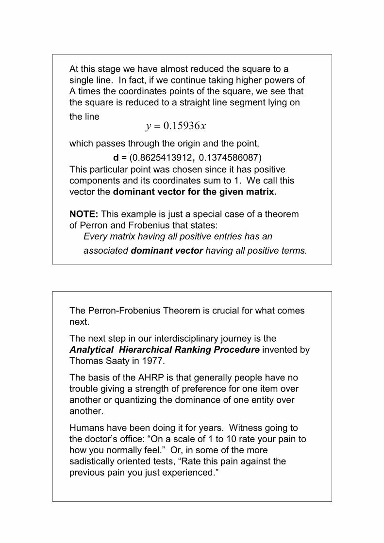
At this stage we have almost reduced the square to a single line. In fact, if we continue taking higher powers of A times the coordinates points of the square, we see that the square is reduced to a straight line segment lying on the line

which passes through the origin and the point, d = (0.8625413912, 0.1374586087)

This particular point was chosen since it has positive components and its coordinates sum to 1. We call this vector the dominant vector for the given matrix.

NOTE: This example is just a special case of a theorem of Perron and Frobenius that states:

Every matrix having all positive entries has an associated dominant vector having all positive terms.

xy 15936.0=

The Perron-Frobenius Theorem is crucial for what comes next.

The next step in our interdisciplinary journey is the Analytical Hierarchical Ranking Procedure invented by Thomas Saaty in 1977.

The basis of the AHRP is that generally people have no trouble giving a strength of preference for one item over another or quantizing the dominance of one entity over another.

Humans have been doing it for years. Witness going to the doctor’s office: “On a scale of 1 to 10 rate your pain to how you normally feel.” Or, in some of the more sadistically oriented tests, “Rate this pain against the previous pain you just experienced.”

We consider the case of serial rapists.

Begin by categorizing different type of rapes:

I. Date Rape or Opportunistic Rape

II. Rape by more than one perpetrator

III. Use of a weapon in subduing victim

IV. Commission of a non-violent crime (burglary) at time of rape.

V. Rape with bodily harm to victim

VI. Rape and murder of the victim

VII. Kidnapping or imprisonment of victim (many times results in death of the victim)

Example of a Rating Sheet(Fill in Columns 2 and 3 only)

Compare Dominant Strength Inverse StrengthI vs III vs IIII vs IVI vs VI vs VII vs VII

II vs IIIo

oo

V vs VIV vs VII

VI vs VIIThere are a total of 21 different pairwise ratings.

How do we determine the value to put in column 3.

Saaty’s guidelines are:

1 = no preference for one item over the other

3 = slightly stronger preference for one over the other

5 = an essential preference for one over the other

7 = some evidence that one is preferred over the other

9 = indisputable evidence for one over the other

Even numbers may be used if the evaluator is undecided between two adjacent categories. A 10 is given if the evidence is Overwhelming in the mind of the evaluator

The following small Derive® 6.1 program finds the dominant vector (all positive entries whose sum = 1) for the matrix related to the seven categories of serial rape. The matrix is called “CM” for Consensus Matrix.

Note that Category VI has the highest ranking (a little over 41%) according to the consensus of the experts.

Geographic Profiling of CriminalsDescribed as: “An investigative support technique for serial violent crime”

Developed at Simon Fraser University in Vancouver, BC, Canada.

Primary work done by Kim Rossmo a student of Paul and Patricia Brantingham at Simon Fraser

Rossmo spent several years as a constable on the Vancouver Police force before attaining his Ph.D. at Simon Fraser

Rossmo is now a private consultant and head of the Center for Geospatial Intelligence and Investigation at Texas State University, San Marcos, Texas

Focus of Geographic Profiling:• geography of the crime • hunting behavior and target selection by perpetrator • relationship to linkage analysis and psychological profiling• crime site topography• case examples from similar cases

The result is not an “X marks the spot,” but, rather, it narrows down the area that most likely contains the home, work area, or other location the perpetrator is likely to frequent.

Rossmo’s Observations

1. Like most animals, humans tend to choose hunting areas that are relatively close to their homes or places they frequent regularly.

2. Because they want anonymity, human hunters tend to establish a buffer zone around their homes and other “haunts.” This is called the “smoke stack effect.”

3. The more violent the crime, the more likely it is that the distance to the crime scene from the buffer zone is greater.

4. It is possible that the crime encounter, attack, and body dump site may all be in one place or may be at different sites

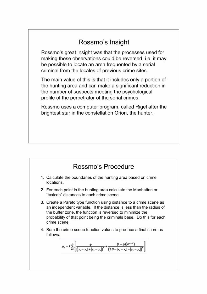
Rossmo’s InsightRossmo’s great insight was that the processes used for making these observations could be reversed, i.e. it may be possible to locate an area frequented by a serial criminal from the locales of previous crime sites.

The main value of this is that it includes only a portion of the hunting area and can make a significant reduction in the number of suspects meeting the psychological profile of the perpetrator of the serial crimes.

Rossmo uses a computer program, called Rigel after the brightest star in the constellation Orion, the hunter.

Rossmo’s Procedure1. Calculate the boundaries of the hunting area based on crime

locations.

2. For each point in the hunting area calculate the Manhattan or “taxicab” distances to each crime scene.

3. Create a Pareto type function using distance to a crime scene asan independent variable. If the distance is less than the radius of the buffer zone, the function is reversed to minimize the probability of that point being the criminals base. Do this for each crime scene.

4. Sum the crime scene function values to produce a final score as follows:

Further Explanation of the FunctionIn Step 4

Problem: Nowhere in my reading could I find any indication of how f, g, and k are determined

Bringing The AHRP and Geographic Profiling Together

1. Point 3 of Rossmo’s observations made brings to mind using the AHRP generated dominant vector.

2. The dominant vector not only gives a ranking, but also assigns a value to the strength of that ranking. For example Category VI is viewed as about 2.7 times as violent as Category V and Category VII is viewed as about 2 times as violent as Category 5 and 1½ times less violent than Category VII.

3. The function ax for 0 < a < 1 decays in much the same way as a Pareto function. NOTE: the larger a the slower the decay.

4. Some adjustment must be made for the Buffer Zone.

5. Use Derive®’s ability to put pictures as background to graphs to place crime scene location maps on the graph and read off coordinates.

The Derive® Working Environment ForThe Lafayette, Louisanna

South Side Rapist

Below is an attempt to find the likely locations for the home ofthe South Side Rapist. The only redeeming feature is that the shaded area does contain two places where the criminal lived. The bad feature is that it does not cut down much on the area to be covered by the investigating team. There is still a need for more work.

The Case of John Duffy

When Duffy started his spree of serial rapes, it was thought that there were 2 rapists. See photo to left.Professor David Cantor of Liverpool University looked at the map below and concentrating on Duffy’s early exploits identified the yellow area below, as does the Derive® procedure to the left.

The Three Rapes Involving MurderNote that the distance from the area included in the first three Duffy rapes is much greater, verifying Rossmo’sobservations. It also justifies the use of a larger base to theexponential. Unfortunately, even this decays too quickly to be of much use.

Jack the RipperBelow are the regions selected for Jack’s home by Rossmo(solid colors) and the results of the Derive® procedures we have been examining. They don’t coincide, but then, no one knows who Jack was or where he lived.

Areas for Much More Research

1. Need to read more criminology research concerning buffer zones and look at published numbers for different types of crimes.

2. Adjust functions to scale of map and assign a constant that will give a more reasonable rate of decay for the exponential functions.

3. Is there a way that the AHRP can be used to determine Rossmo’s constants f, g, and k?

4. Rossmo’s summing of probabilities represents a disjunction. Actually, since we are assuming the crimes are all linked to a single perpetrator, isn’t conjunction the better choice?

Bibliography1. Rossmo, D. Kim, Geographic Profiling, CRC

Press, Bocca Raton, Florida, 2000

2. Cantor, David and Youngs,Donna, Principles of Geographic Offender Profiling, Ashgate Press Limited, Aldershot, Hampshire, UK, 2008

The DERIVE files can be found in folder \TIME08_contribs\Leinbach, editor.