AN ANT COLONY OPTIMIZATION ALGORITHM FOR

JOB SHOP SCHEDULING PROBLEM

Edson Flórez1, Wilfredo Gómez

2 and MSc. Lola Bautista

3

Universidad Industrial de Santander, Bucaramanga, Colombia

1Systems Engineering Student

edson.florez@correo.uis.edu.co 2Systems Engineer, member of the Research Group in Biomedical Engineering

wilfredo.gomez@correo.uis edu.co 3Director of the Research Group in Biomedical Engineering

lxbautis@uis.edu.co

ABSTRACT

The nature has inspired several metaheuristics, outstanding among these is Ant Colony Optimization

(ACO), which have proved to be very effective and efficient in problems of high complexity (NP-hard) in

combinatorial optimization. This paper describes the implementation of an ACO model algorithm known

as Elitist Ant System (EAS), applied to a combinatorial optimization problem called Job Shop Scheduling

Problem (JSSP). We propose a method that seeks to reduce delays designating the operation immediately

available, but considering the operations that lack little to be available and have a greater amount of

pheromone. The performance of the algorithm was evaluated for problems of JSSP reference, comparing

the quality of the solutions obtained regarding the best known solution of the most effective methods. The

solutions were of good quality and obtained with a remarkable efficiency by having to make a very low

number of objective function evaluations.

KEYWORDS

Metaheuristics, Ant Colony Optimization, Swarm intelligence, Combinatorial Optimization, Job Shop

Scheduling Problem.

1. INTRODUCTION

ACO is a metaheuristic that brings together concepts from fields such as Artificial Intelligence and Biology, inspired in the collective behavior of ants. These social insects form colonies of ants, which are self-organizing systems and decentralized which are considered as a Swarm Intelligence [12]. Thanks to that intelligence emerging from simple relationships between ants, a colony can solve complex problems in their environment, such as the problem of finding the shortest path between the colony and the food, which can be used to find the best solution for combinatorial optimization problems.

In this paper, we apply the collective intelligence of many simple agents to the problem of Job Shop Scheduling [22], which consists of finding an optimal plan that minimizes the makespan, which is the time required to perform a finite number of tasks in a finite number of machines

[13]. Each task is a sequence of operations, each one with a determined machine and processing time. Feasible solutions must comply with the restrictions that apply to the problem of Job Shop Scheduling, as respecting the precedence between operations determining the technological sequence without interrupting any operations until completion [21]. The operations conform the graph nodes that represent the problem, united by edges in which ants are moving. Each individual only has local information of the system that shares through a hormone called pheromone.

The update of the pheromone trail deposited on the edges can be done globally or locally. Ants build roads that represent feasible solutions, guided by the pheromone trails and the heuristic

information of each edge [1]. For this reason the ant population performs a stochastic search, selecting the next node to visit only based on information available locally, used on a probabilistic approach where initially the ant decisions are completely random in the absence of pheromone trails.

In the literature, several algorithms have been proposed following the ACO probabilistic technique for finding approximate solutions to complex optimization problems. The first ACO algorithm was Ant System (AS), proposed by Marco Dorigo in 1991 [26], and completed with the contributions of Maniezzo and Colorni [1]. New developments gave better results, like Ant Colony System (ACS) [2], the Max-Min Ant System (MMAS) [7], the Rank-based Ant System (ASrank) [8], among others. This article presents a variant of Elitist Ant System, also proposed by

Dorigo as an improvement to SH [1], applied in JSSP instances widely used known as LA instances, that were raised by Lawrence [11].

2. JSSP PROBLEM FORMULATION

The JSSP or resource planning problem (or jobs) consists in "accommodate resources over time to perform a set of jobs" [6], building plan or execution sequence of jobs j in a set of m machines [13], where an operation is every job that is processed in each machine (Operation(j, m)) and is assigned a specific processing time.

This problem is presented in multiple human activities, taking applications to tasks such as scheduling for packet delivery (eg airway), computer networks (networking), computers (multitasking and multiprocessing), project management (agenda or plan), production and administrative processes (eg assembly lines, etc.) [20].

JSSP must comply with certain restrictions in the execution of jobs and the goal is to complete them in the shortest possible time. This time to optimize is known as makespan (CMAX) or

Maximum Workflow which forms the objective function to minimize given as , where is the job completion time. It is a combinatorial optimization

problem because the number of candidate solutions is combinatorial in size with variables of

discrete nature, therefore the representation of the solutions are permutations over the operations of each job, making it impossible to determine all possible solutions in a reasonable time.

2.1. Computational complexity of JSSP

In 1976 Michael Garey [17] provided evidence that this problem is NP-hard for m> 2, ie cannot be quickly found (polynomial-time) an optimal solution for JSSP with more than two machines. Along with David Johnson in 1979, they finished demonstrating that JSSP is NP-hard [18],

unless in Computational Complexity Theory is proved that P = NP, if so, any problem that can be checked quickly by a computer, it could also be quickly resolved by that computer.

The NP-hard complexity of JSSP lies in the vast number of possible combinations that arise

because each sequence of operations on a machine can be permuted independently of the

sequence of operations on another machine, so with a few jobs and machines can have

possible solutions which corresponds to the search space (S) of the problem.

2.2. Formal definition of Job Shop Scheduling Problem

Having [5]:

: Set of n jobs to be processed.

: Set of m machines or resources.

: Operation of the job that must be processed in the machine by

.

: Uninterrupted period of processing time for each operation.

Objective function: Minimize

Subject to:

Start times restriction for each operation

Precedence constraint if preceding

Disjunctive restriction ( ) if preceding ,

( ) in another case.

Where: , with ∑ ∑

.

The previous set of constraints of the JSSP is explained of this way [21]:

Start restriction: The time when an operation starts are not specified, so work can start at any point in time as long as the required machine is available.

Restriction of precedence: Each job must go through a particular sequence of operations that is predefined, so that operations cannot begin until the end of its predecessor, preventing the processing of two operations of the same job simultaneously.

Restrictions disjunctive: A machine can process only one job at a time. Each operation must be fully processed on a single machine and cannot be interrupted even if there are jobs waiting for that machine to be available, for instance, no work may be processed more than once on the same machine.

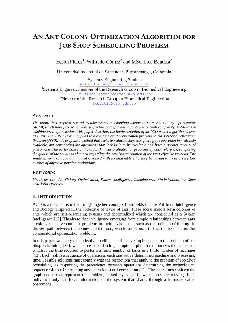
In addition to the above restrictions, we have determined that all operations have the same priority of processing, and all machines are the same and can be idle at any time. The fulfillment of these restrictions can be seen clearly by a Gantt chart (Figure 1), which shows an instance of

JSSP (Table 1) matrix defined by [15], in which it has an additional column to indicate that each row of the matrix corresponds to a job (J1, J2 and J3).

Table 1. An instance of JSSP 3×3

Job (J) Machine (time)

Sequence: S1 S2 S3

J1 3 (4) 2 (3) 1 (3)

J2 2 (1) 3 (2) 1 (4)

J3 2 (3) 1 (2) 3 (3)

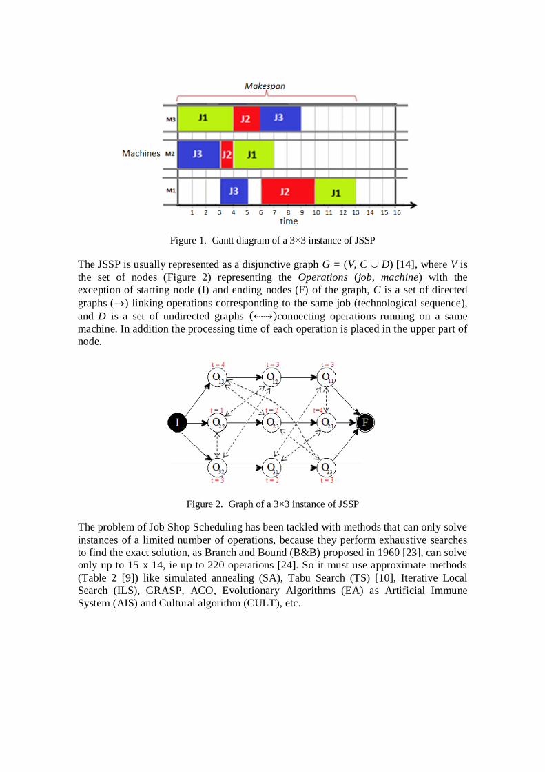
Figure 1. Gantt diagram of a 3×3 instance of JSSP

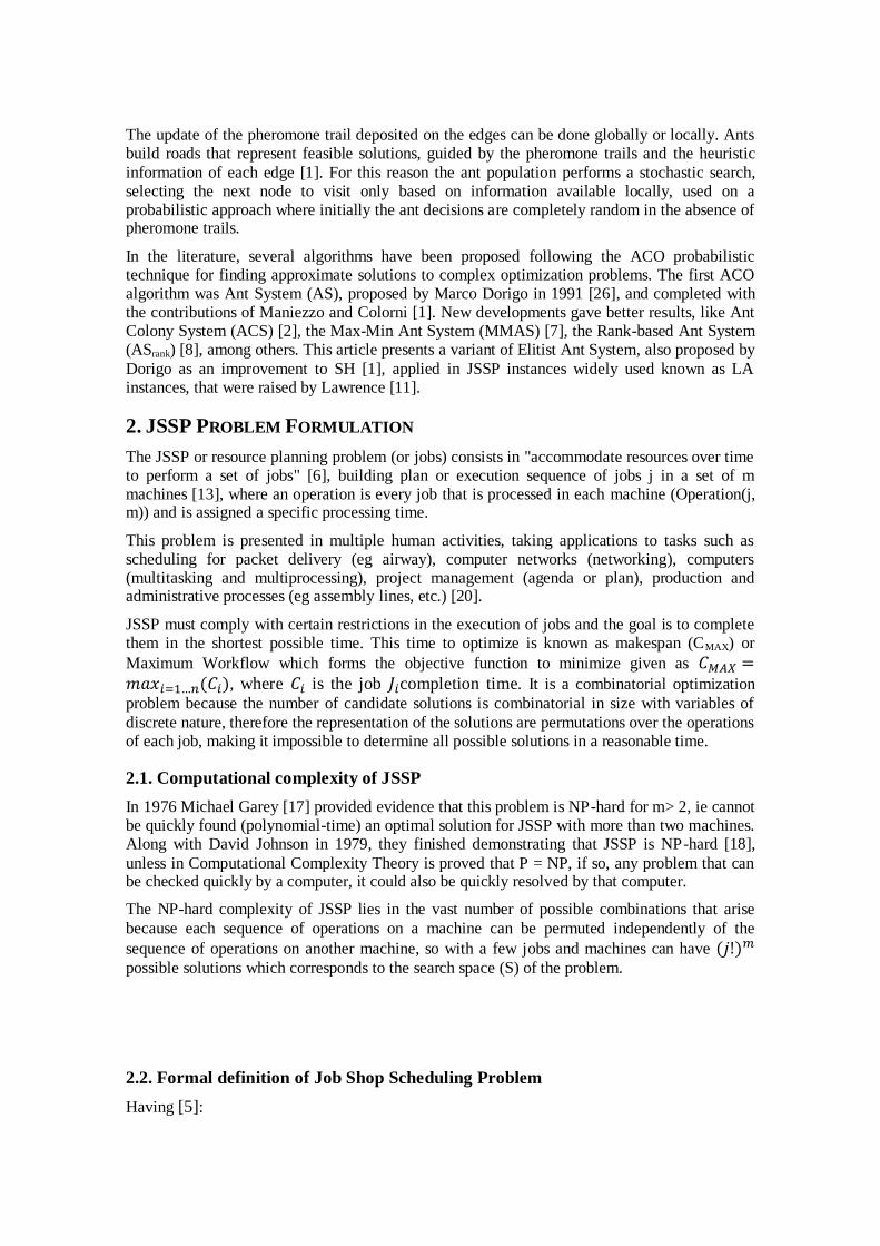
The JSSP is usually represented as a disjunctive graph G = (V, C D) [14], where V is

the set of nodes (Figure 2) representing the Operations (job, machine) with the

exception of starting node (I) and ending nodes (F) of the graph, C is a set of directed

graphs () linking operations corresponding to the same job (technological sequence),

and D is a set of undirected graphs connecting operations running on a same

machine. In addition the processing time of each operation is placed in the upper part of

node.

Figure 2. Graph of a 3×3 instance of JSSP

The problem of Job Shop Scheduling has been tackled with methods that can only solve

instances of a limited number of operations, because they perform exhaustive searches

to find the exact solution, as Branch and Bound (B&B) proposed in 1960 [23], can solve

only up to 15 x 14, ie up to 220 operations [24]. So it must use approximate methods

(Table 2 [9]) like simulated annealing (SA), Tabu Search (TS) [10], Iterative Local

Search (ILS), GRASP, ACO, Evolutionary Algorithms (EA) as Artificial Immune

System (AIS) and Cultural algorithm (CULT), etc.

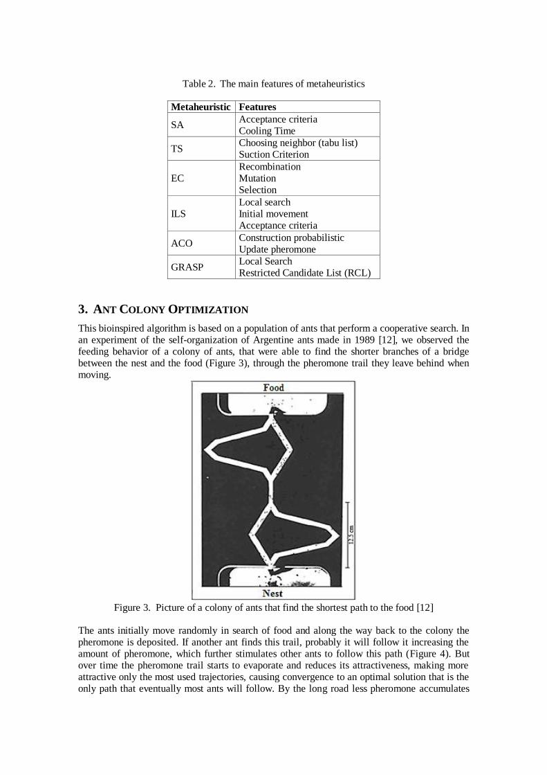
Table 2. The main features of metaheuristics

Metaheuristic Features

SA Acceptance criteria Cooling Time

TS Choosing neighbor (tabu list) Suction Criterion

EC Recombination Mutation Selection

ILS Local search Initial movement Acceptance criteria

ACO Construction probabilistic Update pheromone

GRASP Local Search Restricted Candidate List (RCL)

3. ANT COLONY OPTIMIZATION

This bioinspired algorithm is based on a population of ants that perform a cooperative search. In an experiment of the self-organization of Argentine ants made in 1989 [12], we observed the feeding behavior of a colony of ants, that were able to find the shorter branches of a bridge between the nest and the food (Figure 3), through the pheromone trail they leave behind when moving.

Figure 3. Picture of a colony of ants that find the shortest path to the food [12]

The ants initially move randomly in search of food and along the way back to the colony the pheromone is deposited. If another ant finds this trail, probably it will follow it increasing the amount of pheromone, which further stimulates other ants to follow this path (Figure 4). But over time the pheromone trail starts to evaporate and reduces its attractiveness, making more attractive only the most used trajectories, causing convergence to an optimal solution that is the only path that eventually most ants will follow. By the long road less pheromone accumulates

because of the low passing frequency of the ants when they spend more time completing their road.

Figure 4. A. ants in a pheromone trail between nest and food; B. an obstacle interrupts the trail; C. ants find two paths to go around the obstacle; D. a new pheromone trail is formed along the

shorter path [19]

In the ACO algorithms family, ant’s behavior is simulated with a virtual agent that has the capacity to explore a limited search space and obtain information about the surrounding environment. The artificial ant (k) moves from one node to another (from source node i to destination node j), building step by step solution to be written to the Tabuk memory (that stores

information about the nodes sequence or route taken until time t), that ends when it reaches one of the accepting states defined by the objective of the problem.

Thus, the ants can construct approximate solutions to complex problems such as sequencing,

assigning, planning or programming. Each edge of the graph has two types of associated information that guide the movement of the ant [4] and whose values are modified by ants at each iteration:

ij Heuristic information that measures the heuristics preference of moving from node i to node j, when touring the edge aij. Ants do not change this information during the execution of the algorithm.

ij Information of artificial pheromone trails, that measures the "desirability learned" of the i to j movement. This information is modified during the execution of the algorithm depending on the solutions found by the ants to reflect the experience gained by these agents.

Pseudocode of the ACO metaheuristic [3]: ACO procedure Set parameters,Initialize the pheromone trails

scheduled activities Construction of solutions by ants

Server of actions (Optional) Updating pheromone

End-Scheduled activities End-procedure

The metaheuristic consists of a parameter initialization step and three algorithmic procedures whose activation is regulated by the builder Scheduled activities, in which is repeated until a termination condition is met, such as reaching a maximum number of iterations or a maximum CPU time. The three algorithmic procedures submitted to the Scheduled activities consist of [25]:

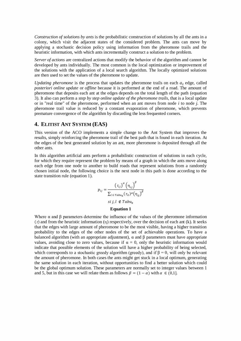
Construction of solutions by ants is the probabilistic construction of solutions by all the ants in a colony, which visit the adjacent states of the considered problem. The ants can move by

applying a stochastic decision policy using information from the pheromone trails and the heuristic information, with which ants incrementally construct a solution to the problem.

Server of actions are centralized actions that modify the behavior of the algorithm and cannot be

developed by ants individually. The most common is the local optimization or improvement of the solutions with the application of a local search algorithm. The locally optimized solutions are then used to set the values of the pheromone to update.

Updating pheromone is the process that updates the pheromone trails on each aij edge, called posteriori online update or offline because it is performed at the end of a road. The amount of pheromone that deposits each ant at the edges depends on the total length of the path (equation 3). It also can perform a step by step online update of the pheromone trails, that is a local update or in "real time" of the pheromone, performed when an ant moves from node i to node j. The pheromone trail value is reduced by a constant evaporation of pheromone, which prevents premature convergence of the algorithm by discarding the less frequented corners.

4. ELITIST ANT SYSTEM (EAS)

This version of the ACO implements a simple change to the Ant System that improves the results, simply reinforcing the pheromone trail of the best path that is found in each iteration. At

the edges of the best generated solution by an ant, more pheromone is deposited through all the other ants.

In this algorithm artificial ants perform a probabilistic construction of solutions in each cycle, for which they require represent the problem by means of a graph in which the ants move along each edge from one node to another to build roads that represent solutions from a randomly chosen initial node, the following choice is the next node in this path is done according to the state transition rule (equation 1).

( )

(

)

∑ ( )

Equation 1

Where α and β parameters determine the influence of the values of the pheromone information and from the heuristic information () respectively, over the decision of each ant (k). It seeks that the edges with large amount of pheromone to be the most visible, having a higher transition probability to the edges of the other nodes of the set of achievable operations. To have a balanced algorithm (with an appropriate adjustment), α and β parameters must have appropriate

values, avoiding close to zero values, because if α = 0, only the heuristic information would indicate that possible elements of the solution will have a higher probability of being selected, which corresponds to a stochastic greedy algorithm (greedy), and if β = 0, will only be relevant the amount of pheromone. In both cases the ants might get stuck in a local optimum, generating the same solution in each iteration, without opportunities to find a better solution which could be the global optimum solution. These parameters are normally set to integer values between 1 and 5, but in this case we will relate them as follows with .

The amount of pheromone present at each edge of the road in the generation is given by

the equation 2.

∑

Equation 2

Where is the contribution of the ant to the total pheromone of the generation and is

the evaporation rate of the pheromone. The reason for including the evaporation rate is that old pheromone should not have much influence on future decisions of the ants. The amount of pheromone that each ant is contributing depends on the quality of the solution obtained which is inversely proportional to the cost of the solution of the objective function (equation 3).

Equation 3

Where is a constant and is the length of the makespan of the solution obtained by the ant.

To accelerate the convergence of the algorithm, increasing the visibility of the pheromone trail on all edges of the shortest path, passing all elitists ants (e) of the system. Therefore, the equation 3 for the best path built in each cycle is replaced by the equation 2.

Equation 4

5. EAS IMPLEMENTATION FOR JSSP

The rapid convergence of this algorithm can reduce the scanning capability since the ants soon will end in a single way, which can be a local optimum. To compensate this, is allowed to include in the set of achievable operations (point 3.3 of pseudocode), operations that makes the machines wait (on pause) some units of time to begin execution because the corresponding job is still active on another machine. But this operation that delay or retards the onset of the machines will only be selected if the edge that reaches the node, has enough pheromone to make

the probability to be greater than the operations that have immediately available jobs. That will only be given with large amounts of pheromone, because having idle machines is not adequate and is penalized lowering the visibility of the operation.

This method further explores the search space in order to obtain many solutions, from which it can be obtained solutions that exceed the local optima found in the first iterations. These optimal are the ones limiting the search, stopping it on solutions distant up to a 5% the global optimum. The initial diversity of the algorithm is the one that ensures that the ants move towards the search space where the path corresponding to the overall optimal solution is found. The following is the pseudocode implemented to solve the JSSP:

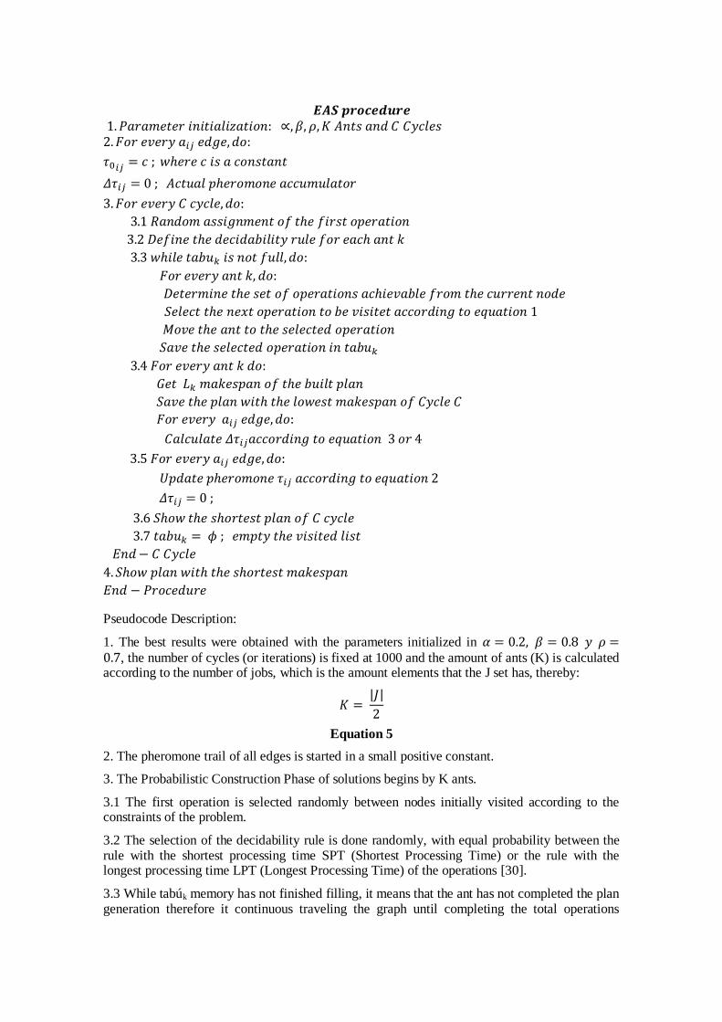
Pseudocode Description:

1. The best results were obtained with the parameters initialized in , the number of cycles (or iterations) is fixed at 1000 and the amount of ants (K) is calculated according to the number of jobs, which is the amount elements that the J set has, thereby:

| |

Equation 5

2. The pheromone trail of all edges is started in a small positive constant.

3. The Probabilistic Construction Phase of solutions begins by K ants.

3.1 The first operation is selected randomly between nodes initially visited according to the constraints of the problem.

3.2 The selection of the decidability rule is done randomly, with equal probability between the rule with the shortest processing time SPT (Shortest Processing Time) or the rule with the longest processing time LPT (Longest Processing Time) of the operations [30].

3.3 While tabúk memory has not finished filling, it means that the ant has not completed the plan generation therefore it continuous traveling the graph until completing the total operations

(| | | | | |). The tabuk list restricts the choice of operations to prevent a return to recently

visited nodes. In the set of visited operations are included operations that generate a delay in the machines less or equal to five time units. To maintain the balance affected by the delay generated, visibility of the node is reduced on a percentage point per unit of time lost.

3.4 Once each ant has built a solution, the pheromone actualization process is started, reviewing the traveled path to add the appropriate amount of pheromone according to equation 3 or 4, to the pheromone accumulator of the current cycle. If the makespan of the solution is expensive, less importance is given to the way, thus depositing few pheromone on edges.

3.5 Update pheromone trails of the visited edges using a process known as posteriori online update, which is a global update performed offline, that is, after the execution of each cycle of

the algorithm. It is deposited in the pheromone trails of each of the edges of the graph, what the ants have been added in the respective pheromone accumulator. Then the actual pheromone accumulator is restarted at zero for not to redeposit this pheromone in the next cycle.

3.6 The best quality plan of the current cycle is saved with its respective makespan.

3.7 Memory (tabuk) is erased on each ant to start building new plans in the next cycle.

4. Shows the best plan of all cycles performed by the algorithm.

6. ANALYSIS AND COMPARISON OF RESULTS

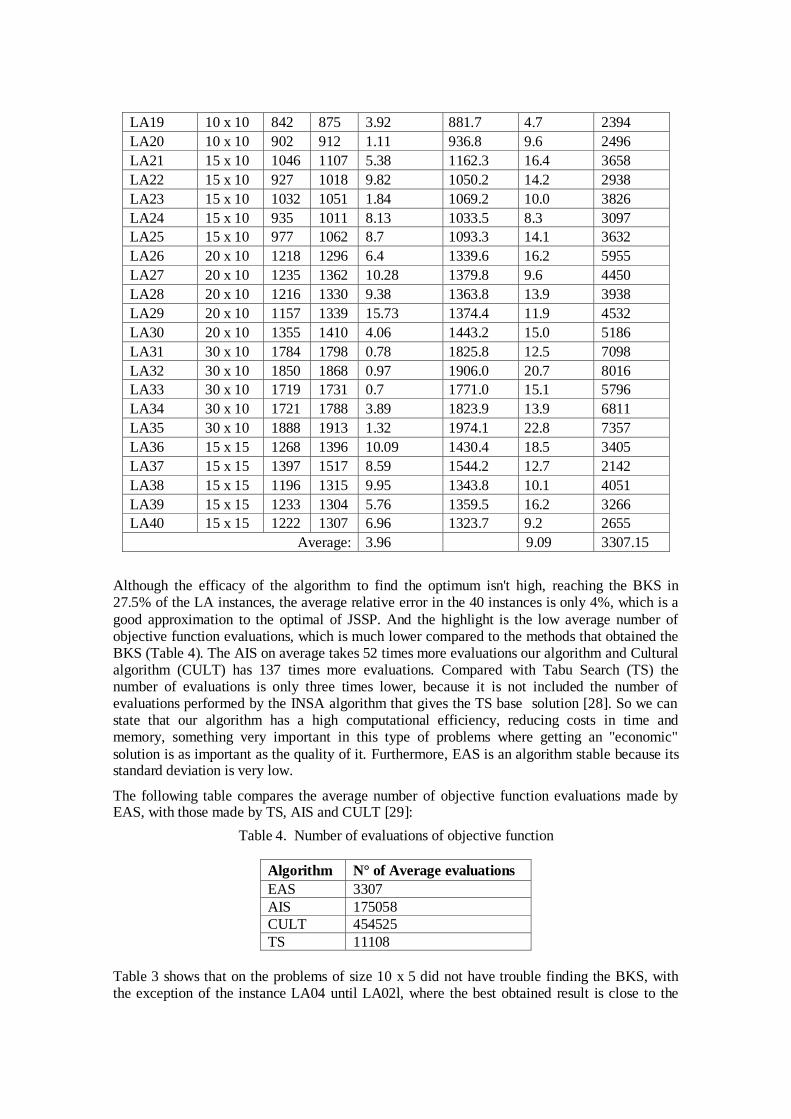
Results shown in Table 3 were obtained in 30 executions of the algorithm (1000 iterations) for each of the 40 JSSP instances raised by Lawrence [11], that are of different sizes and difficulty, and because of its wide use, we can compare the results with other techniques that generate the

best known solution (BKS) taken from [13] and [27] The table shows, the name of the instance of Lawrence, its size and BKS, the best makespan found and their percentage relative error respect al BKS, the makespan average, standard deviation, and finally the average number of evaluations of the objective function.

Table 3. Experimental results

Instance Size BKS Best

Cmax

Relative

Error (%)

Cmax

Average

Standard

deviation

#Eval.

Average

LA01 10 x 5 666 666 0 667.8 2.3 2375

LA02 10 x 5 655 669 2.13 689.7 6.2 2809

LA03 10 x 5 597 623 4.36 644.8 8.0 2230

LA04 10 x 5 590 611 3.56 617.7 5.0 2257

LA05 10 x 5 593 593 0 593.0 0.0 101

LA06 15 x 5 926 926 0 926.0 0.0 531

LA07 15 x 5 890 890 0 898.2 5.6 3443

LA08 15 x 5 863 863 0 863.1 0.4 2251

LA09 15 x 5 951 951 0 951.0 0.0 391

LA10 15 x 5 958 958 0 958.0 0.0 637

LA11 20 x 5 1222 1222 0 1222.0 0.0 1504

LA12 20 x 5 1039 1039 0 1039.0 0.0 1752

LA13 20 x 5 1150 1150 0 1150.0 0.2 2952

LA14 20 x 5 1292 1292 0 1292.0 0.0 471

LA15 20 x 5 1207 1212 0.41 1245.6 9.9 3836

LA16 10 x 10 945 1005 6.35 1020.1 10.1 2700

LA17 10 x 10 784 812 3.57 836.1 10.9 2401

LA18 10 x 10 848 885 4.36 904.8 9.8 2946

LA19 10 x 10 842 875 3.92 881.7 4.7 2394

LA20 10 x 10 902 912 1.11 936.8 9.6 2496

LA21 15 x 10 1046 1107 5.38 1162.3 16.4 3658

LA22 15 x 10 927 1018 9.82 1050.2 14.2 2938

LA23 15 x 10 1032 1051 1.84 1069.2 10.0 3826

LA24 15 x 10 935 1011 8.13 1033.5 8.3 3097

LA25 15 x 10 977 1062 8.7 1093.3 14.1 3632

LA26 20 x 10 1218 1296 6.4 1339.6 16.2 5955

LA27 20 x 10 1235 1362 10.28 1379.8 9.6 4450

LA28 20 x 10 1216 1330 9.38 1363.8 13.9 3938

LA29 20 x 10 1157 1339 15.73 1374.4 11.9 4532

LA30 20 x 10 1355 1410 4.06 1443.2 15.0 5186

LA31 30 x 10 1784 1798 0.78 1825.8 12.5 7098

LA32 30 x 10 1850 1868 0.97 1906.0 20.7 8016

LA33 30 x 10 1719 1731 0.7 1771.0 15.1 5796

LA34 30 x 10 1721 1788 3.89 1823.9 13.9 6811

LA35 30 x 10 1888 1913 1.32 1974.1 22.8 7357

LA36 15 x 15 1268 1396 10.09 1430.4 18.5 3405

LA37 15 x 15 1397 1517 8.59 1544.2 12.7 2142

LA38 15 x 15 1196 1315 9.95 1343.8 10.1 4051

LA39 15 x 15 1233 1304 5.76 1359.5 16.2 3266

LA40 15 x 15 1222 1307 6.96 1323.7 9.2 2655

Average: 3.96 9.09 3307.15

Although the efficacy of the algorithm to find the optimum isn't high, reaching the BKS in 27.5% of the LA instances, the average relative error in the 40 instances is only 4%, which is a

good approximation to the optimal of JSSP. And the highlight is the low average number of objective function evaluations, which is much lower compared to the methods that obtained the BKS (Table 4). The AIS on average takes 52 times more evaluations our algorithm and Cultural algorithm (CULT) has 137 times more evaluations. Compared with Tabu Search (TS) the number of evaluations is only three times lower, because it is not included the number of evaluations performed by the INSA algorithm that gives the TS base solution [28]. So we can state that our algorithm has a high computational efficiency, reducing costs in time and memory, something very important in this type of problems where getting an "economic"

solution is as important as the quality of it. Furthermore, EAS is an algorithm stable because its standard deviation is very low.

The following table compares the average number of objective function evaluations made by EAS, with those made by TS, AIS and CULT [29]:

Table 4. Number of evaluations of objective function

Algorithm N° of Average evaluations

EAS 3307

AIS 175058

CULT 454525

TS 11108

Table 3 shows that on the problems of size 10 x 5 did not have trouble finding the BKS, with the exception of the instance LA04 until LA02l, where the best obtained result is close to the

BKS (less than 5%). Also for instances of size 15 x 5 and 20 x 5, with the exception of the LA15 that only moves away from BKS in 5 units of time. In the other instances (size 10 x 10,

15 x 10, 20 x 10, 30 x 10 and 15 x 15), which have 5 or 10 machines more than the previous, complexity is quite high because of the considerable number of operations to be performed, this means lower quality solutions obtained. For example, to instances of size 30 x 10, 300 operations must be performed, and the total number of possible combinations is (30!)10, that is approximately 2.65 x 1042. However, the algorithm achieves to present high quality solutions on instances of 30 x 10 (Figure 5). In general, 65% of executed instances approaches less than 5% of BKS and 47.5% deviate by less than 3% of the BKS.

Figure 5. Relative Error average by instance size

7. CONCLUSIONS

The Ant Colony Optimization is a technique of swarm intelligence, which is applied for

combinatorial optimization problems as JSSP. The algorithm implemented, Elitist Ant System, has proven to be competitive by find good quality solutions to JSSP in a low number of objective function evaluations, although requires improvements to obtain the best known solution in all LA instances. Therefore, ACO is a metaheuristic that has the potential to obtain efficiently solutions of scheduling problems, with minimal cost of time and computational resources.

REFERENCES

[1] M. Dorigo, V. Maniezzo, and V.M. Colorni, “The Ant System: Optimization by a colony of

cooperating agents,” IEEE: Transactions on Systems, Man, and Cybernetics, Part B, vol. 26, no.

1, pp. 29-41, 1996.

[2] M. Dorigo and L.M. Gambardella, “Ant Colony System: A cooperative learning approach to the

Traveling Salesman Problem,” IEEE: Transactions on Evolutionary Computation, vol. 1, no. 1,

pp. 53-66, 1997.

[3] M. Dorigo and K. Socha, “An introduction to Ant Colony Optimization,” Technicalreport N° 10

of the Institut de RecherchesInterdisciplinaires et de Développements en IntelligenceArtificielle

(IRIDIA), Université Libre de Bruxelles, Belgium, 2006.

0

1

2

3

4

5

6

7

8

9

10

10 x 5 15 x 5 20 x 5 10 x 10 15 x 10 20 x 10 30 x 10 15 x 15

Per

centa

ge

rela

tive

erro

r a

ver

age

Instance Size

EAS

[4] S. Alonso, O. Cordón, I. Fernández, and F. Herrera F,“La metaheurística de Optimización

basada en Colonias de Hormigas: Modelos y nuevos enfoques,” Trabajo realizado en el marco

del proyecto Mejora de Metaheurísticas mediante Hibridación y sus Aplicaciones, de la

Universidad de Granada, España, 2004.

[5] V. Peña and L. Zumelzu, Estado del arte del Job Shop Scheduling Problem, Departamento de

Informática, Universidad Técnica Federico Santa María Valparaíso, Chile, 2006.

[6] J. Blazewicz, K. H. Ecker, G. Schmidt, and J. Weglarz. Scheduling in Computer and

Manufacturing System. Springer, 1994.

[7] T. Stützle and H.H. Hoos, “MAX-MIN Ant System”. Future Generation Computer Systems,vol.

16, no. 8, pp. 889-914, 2000.

[8] B. Bullnheimer, R.F. Hartl, and C. Strauss, “A New Rank-Based version of the Ant System: A

computational study,” Central European Journal for Operations Research and Economics,vol. 7,

no. 1, pp. 25-38, 1999.

[9] C. Blum and A. Roli, “Metaheuristics in combinatorial optimization: Overview and conceptual

comparison,” ACM Computing Surveys, vol. 35, no. 3, pp. 268-308, 2003.

[10] M. Ben-Daya and M.Al-Fawzan, A tabu search approach for the flow shop scheduling problem.

InEuropean Journal of Operational Research, vol. 109, pp. 88-95, 1998.

[11] S. Lawrence, ”Resource constrained project scheduling: an experimental investigation of

heuristic scheduling techniques”,In Graduate School of Industrial Administration, Carnegie

Mellon University, Pittsburgh, Pennsylvania, 1984.

[12] S. Goss, S. Aron, J. Deneubourg,and J. Pasteels,“Self-organized shortcuts in the Argentine

ant,”Naturwissenschaften,vol. 76, no.12, pp. 579-581, 1989.

[13] D. Applegate and W. Cook, “A computational study of the job-shop scheduling problem,” In

ORSA Journal on Computing, vol. 3, No. 2, pp. 149–156, 1991.

[14] R. J. M. Vaessens, E. H. L. Aarts, and J. K. Lenstra,“Job Shop Scheduling by Local Search,” INFORMS J. Comput., vol. 8, no. 3, pp. 302–317, 1996.

[15] M. Ventresca and B. M. Ombuki, “Ant Colony Optimization for Job Shop Scheduling Problem,”

Tech. Rep. N° CS-04-04, Department of Computer Science, Brock University, 2004.

[16] O. Cordon, Sistemas Complejos, Algoritmos Evolutivos y Bioinspirados. Universidad de

Granada, España, 2005.

[17] M. R. Garey, “The complexity of Flowshop and Job Shop Scheduling,” Mathematics of

Operations Research, vol. 1, no. 2, pp. 117–129, 1976.

[18] M. R. Garey and D. S. Johnson, Computers and Intractability: A Guide to the Theory of NP-

Completeness, 1979.

[19] M. Perretto and S. Lopes, Reconstruction of phylogenetic trees using the ant colony optimization

paradigm. Genetics and Molecular Research, 4(3), pp. 581-589, 2005.

[20] V. A. Peña, Cadena de Suministros: sus niveles e importancia. Modelado de Procesos de

Negocios, 2006.

[21] A. Manne, “On the Job-Shop Scheduling Problem”, Operations Research, vol. 8, no. 2, pp. 219-

223, 1960.

[22] J. L. Denebourg, J. M. Pasteels, and J.C. Verhaeghe, “Probabilistic behaviour in ants: a strategy

of errors?”, Journal of Theoretical Biology, no. 105, 1983.

[23] A. H. Land and A. G. Doig, “An automatic method of solving discrete programming problems”.

Econometrica, vol. 28, no 3, pp. 497–520, 1960.

[24] T. Yamada and R. Nakano. Job-shop scheduling. In P. J. Fleming A. M. S. Zalzala, editor,

Genetic Algorithms in Engineering Systems, chapter 7, pp. 134–160. IET, 1999.

[25] M. Dorigo and T. Stützle, Ant Colony Optimization. Cambridge, Massachusetts, USA: The MIT

Press, 2004.

[26] M. Dorigo, Optimization, Learning and Natural Algorithms. Ph.D.Thesis, Politecnico di Milano,

Italy, 1992.

[27] C. Coello Coello, D. Cortez Rivera, and N. Cruz Cortez, “Use of an artificial immune system for

job shop scheduling,” in Artificial Immune Systems,” Proceedings of ICARIS, Lecture Notes in

Computer Science vol. 2787, pp. 1–10, 2003.

[28] E. Nowicki and C. Smutnicki, “A fast taboo search algorithm for the job shop problem,”

Management Science, vol. 42, no. 6, pp. 797–813, 1996.

[29] E. Téllez, Uso de una Colonia de Hormigas para resolver Problemas de programación de

Horarios, 2007.

[30] A. Colorni, M. Dorigo, V. Maniezzo and M. Trubian. Ant system for job-shop scheduling.

Belgian Journal of Operations Research, Statistics and Computer Science, 34(1), pp. 39-53,

1994.

Authors

Edson Flórez was born at San

Gil (Colombia) in 1991, is currently

an engineer student at School of

Engineering and Computing Systems

of the Universidad Industrial de

Santander. His research areas are on

Swarm Intelligence algorithms,

Operations Research and Distributed

systems.

Wilfredo Gómez was born at

Bucaramanga(Colombia) in 1984, is

currently an Magister candidate in

system engineering at School of

Engineering and Computing Systems

of the Universidad Industrial de

Santander. His research areas are on

Bioinspired Computation, Operations

Research and Education.

Lola Bautista is MSc. in Computer

Engineering University of Puerto Rico

she is currently the Director of the

Research Group in Biomedical

Engineering. His research areas are on

Software Design in Cardiology and

Electrocardiography, Digital Signal

Processing and Graphics, Data

Mining.