An Analytical Least-Squares Solution to theLine Scan LIDAR-Camera Extrinsic Calibration Problem

Chao X. Guo and Stergios I. Roumeliotis

Abstract— In this paper, we present an elegant solution to the2D LIDAR-camera extrinsic calibration problem. Specifically,we develop a simple method for establishing correspondencesbetween a line-scan (2D) LIDAR and a camera using a smallcalibration target that only contains a straight line. Moreover,we formulate the nonlinear least-squares problem for findingthe unknown 6 degree-of-freedom (dof) transformation betweenthe two sensors, and solve it analytically to determine its globalminimum. Additionally, we examine the conditions under whichthe unknown transformation becomes unobservable, which canbe used for avoiding ill-conditioned configurations. Finally, wepresent extensive simulation and experimental results for assess-ing the performance of the proposed algorithm as compared toalternative analytical approaches.

I. INTRODUCTION AND RELATED WORK

LIDAR-camera systems are widely used in various roboticapplications primarily due to their complementary sensingcapabilities. For instance, the camera’s scale ambiguity canbe determined from the LIDAR measurements, while mo-tion estimates from the camera can be used for findingcorrespondences between two LIDAR scans. Additionally,when combining information from both sensors one canachieve higher motion-estimation accuracy. Fusing, however,measurements from a LIDAR and a camera requires preciseknowledge of the 6 dof transformation between them. Since2D LIDARs are more widely used due to their significantlylower cost and size, we hereafter focus on 2D LIDAR-cameracalibration methods.1

An approximate least-squares solution to the 2D LIDAR-camera extrinsic calibration problem is presented in [5].Specifically, the authors first determine the camera’s posewith respect to a checkerboard using the PnP algorithm [6],and define a geometric constraint relating the LIDAR andcamera measurements on the checkerboard (the camera-checkerboard distance equals the projection of the LIDARpoints onto the checkerboard’s normal vector). Using thisgeometric constraint, a linear least-squares problem is formu-lated by defining, as a new variable, a nonlinear quadratic

The authors are with the Department of Computer Science & En-gineering, University of Minnesota, Minneapolis, MN 55455, USA{chaguo|stergios}@cs.umn.edu

This work was supported by the University of Minnesota through theDigital Technology Center (DTC), and the National Science Foundation(IIS-0835637).

1Note that existing 3D LIDAR-camera extrinsic calibration methodscannot be used since they rely on 3D LIDAR measurements for findingthe normal vector to a calibration target [1], [2], or aligning LIDAR depthdiscontinuities with image edges [3], which is not possible when usinga 2D LIDAR. While this is not an issue for [4], the complexity of thecalibration problem when using 3D LIDAR measurements requires makingcertain approximations (see [4] for more details) which are not necessarywhen using a 2D LIDAR.

term which embeds both the unknown rotation and trans-lation. However, the proposed method is suboptimal sinceits solution does not directly satisfy the rotational matrixconstraint. Therefore, the computed rotation has to be ap-proximated by projecting the obtained solution on the specialorthogonal group, SO(3).

The work described in [7], provides an analytical solutionto the minimal LIDAR-camera calibration problem (i.e.,using six LIDAR and camera measurement sets). In orderto facilitate data association, a calibration board containingwhite and black bands is used. The transition line betweenthe white and black bands is detected by both the camera(using image processing techniques) and the LIDAR (basedon the differences in reflection intensities). Using thesematches, geometric constraints are formed (the LIDAR-measured 3D points on a transition line belong to the planedefined by the transition line detected in the image and thecamera’s center) and solved analytically. This deterministicmethod, however, does not compute the optimal least-squaressolution. Moreover, it is sensitive to noise. Thus, when morethan the minimum required number of measurements areavailable, it must be used in conjunction with RANSAC [8]so as to improve its robustness to noise.

The work described in this paper, makes the followingmain contributions:

• We introduce a simple, yet powerful, calibration pro-cedure, where the calibration target used only containsa straight line. Moreover, we do not require measuringthe laser intensity which makes our method applicableto a wider range of LIDARs.

• We formulate the LIDAR-camera extrinsic calibrationproblem as a least-squares minimization problem andsolve it analytically to find the optimal values for the6 dof unknown transformation.

• We investigate the conditions under which the LIDAR-camera transformation becomes (un)observable.

• We validate the accuracy of our approach both insimulations and experimentally, and demonstrate theperformance improvement as compared to the analyticalapproach of [7].

The rest of the paper is structured as follows. In Section II,we describe our calibration setup and formulate the least-squares problem for finding the LIDAR-camera calibrationparameters. We present the details of our analytical solutionin Section III, while Section IV describes our observabilityanalysis. Sections V and VI present the simulation andexperimental validation of the proposed algorithm, respec-

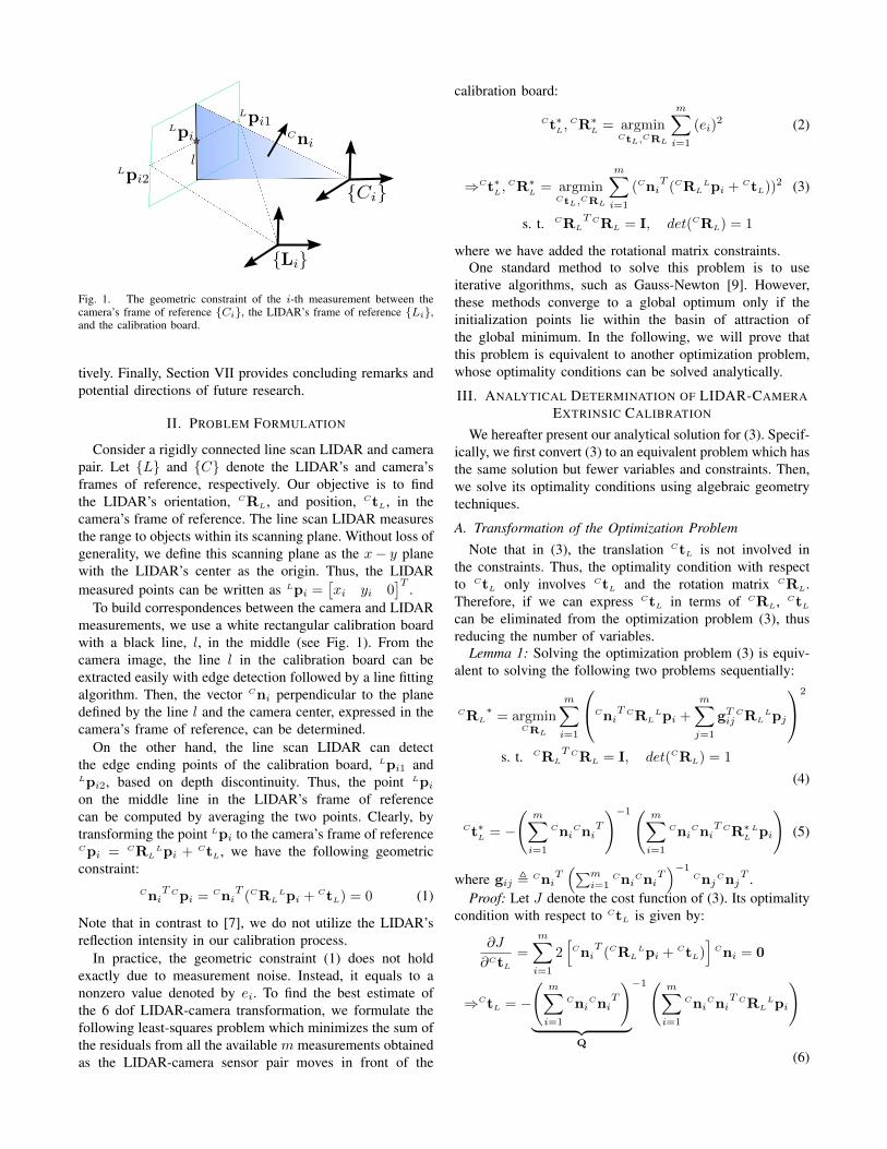
Fig. 1. The geometric constraint of the i-th measurement between thecamera’s frame of reference {Ci}, the LIDAR’s frame of reference {Li},and the calibration board.

tively. Finally, Section VII provides concluding remarks andpotential directions of future research.

II. PROBLEM FORMULATION

Consider a rigidly connected line scan LIDAR and camerapair. Let {L} and {C} denote the LIDAR’s and camera’sframes of reference, respectively. Our objective is to findthe LIDAR’s orientation, CRL, and position, CtL, in thecamera’s frame of reference. The line scan LIDAR measuresthe range to objects within its scanning plane. Without loss ofgenerality, we define this scanning plane as the x− y planewith the LIDAR’s center as the origin. Thus, the LIDARmeasured points can be written as Lpi =

[xi yi 0

]T.

To build correspondences between the camera and LIDARmeasurements, we use a white rectangular calibration boardwith a black line, l, in the middle (see Fig. 1). From thecamera image, the line l in the calibration board can beextracted easily with edge detection followed by a line fittingalgorithm. Then, the vector Cni perpendicular to the planedefined by the line l and the camera center, expressed in thecamera’s frame of reference, can be determined.

On the other hand, the line scan LIDAR can detectthe edge ending points of the calibration board, Lpi1 andLpi2, based on depth discontinuity. Thus, the point Lpion the middle line in the LIDAR’s frame of referencecan be computed by averaging the two points. Clearly, bytransforming the point Lpi to the camera’s frame of referenceCpi = CRL

Lpi + CtL, we have the following geometricconstraint:

CniT Cpi = Cni

T(CRL

Lpi + CtL) = 0 (1)

Note that in contrast to [7], we do not utilize the LIDAR’sreflection intensity in our calibration process.

In practice, the geometric constraint (1) does not holdexactly due to measurement noise. Instead, it equals to anonzero value denoted by ei. To find the best estimate ofthe 6 dof LIDAR-camera transformation, we formulate thefollowing least-squares problem which minimizes the sum ofthe residuals from all the available m measurements obtainedas the LIDAR-camera sensor pair moves in front of the

calibration board:

Ct∗L,CR∗L = argmin

CtL,CRL

m∑i=1

(ei)2 (2)

⇒Ct∗L,CR∗L = argmin

CtL,CRL

m∑i=1

(CniT

(CRLLpi + CtL))2 (3)

s. t. CRL

T CRL = I, det(CRL) = 1

where we have added the rotational matrix constraints.One standard method to solve this problem is to use

iterative algorithms, such as Gauss-Newton [9]. However,these methods converge to a global optimum only if theinitialization points lie within the basin of attraction ofthe global minimum. In the following, we will prove thatthis problem is equivalent to another optimization problem,whose optimality conditions can be solved analytically.

III. ANALYTICAL DETERMINATION OF LIDAR-CAMERAEXTRINSIC CALIBRATION

We hereafter present our analytical solution for (3). Specif-ically, we first convert (3) to an equivalent problem which hasthe same solution but fewer variables and constraints. Then,we solve its optimality conditions using algebraic geometrytechniques.

A. Transformation of the Optimization ProblemNote that in (3), the translation CtL is not involved in

the constraints. Thus, the optimality condition with respectto CtL only involves CtL and the rotation matrix CRL.Therefore, if we can express CtL in terms of CRL, CtL

can be eliminated from the optimization problem (3), thusreducing the number of variables.

Lemma 1: Solving the optimization problem (3) is equiv-alent to solving the following two problems sequentially:

CRL

∗= argmin

CRL

m∑i=1

CniT CRL

Lpi +

m∑j=1

gTijCRL

Lpj

2

s. t. CRL

T CRL = I, det(CRL) = 1

(4)

Ct∗L = −

(m∑i=1

CniCni

T

)−1( m∑i=1

CniCni

T CR∗LLpi

)(5)

where gij , CniT(∑m

i=1Cni

CniT)−1

CnjCnj

T .Proof: Let J denote the cost function of (3). Its optimality

condition with respect to CtL is given by:

∂J

∂CtL

=

m∑i=1

2[Cni

T(CRL

Lpi + CtL)]

Cni = 0

⇒CtL = −

(m∑i=1

CniCni

T

)︸ ︷︷ ︸

Q

−1( m∑i=1

CniCni

T CRLLpi

)

(6)

Substituting (6) in the cost function of (3), we have:

J =

m∑i=1

[Cni

T CRLLpi − Cni

TQ−1(

m∑j=1

CnjCnj

T CRLLpj)

]2

=

m∑i=1

[Cni

T CRLLpi − (

m∑j=1

CniTQ−1Cnj

CnjT CRL

Lpj)

]2

=

m∑i=1

(Cni

T CRLLpi +

m∑j=1

gTij

CRLLpj

)2

(7)

Minimizing (7) with respect to CRL yields CR∗L, and substi-tuting CR∗L into (6) results in (5). This completes the proof.�

To further simplify problem (4), we choose to use thequaternion representation for the rotation matrix CRL, in-stead of the Cayley-Gibbs-Rodriguez parameterization [10]as in [4], which has a singular configuration when therotation angle is π. For more details, we refer the interestedreader to [10]. In particular, problem (4) is simplified byapplication of the following Lemma:

Lemma 2: Using the quaternion representation CLq for the

rotation matrix CRL, problem (4) is equivalent to:

C

Lq∗ = argmin

CLq

m∑i=1

(C

LqTMi

C

Lq)2

(8)

s. t. C

LqT C

Lq = 1

where

Mi , L(Cni)TR(Lpi) +

m∑j=1

L(gij)TR(Lpj) (9)

In the above expression, x denotes the quaternion form of avector x, while L(·) and R(·) are left and right quaternionmultiplication matrices (see Appendix I).

Proof: Using quaternion parameterization, the cost func-tion of (4) can be written as:

J =m∑

i=1

CnTi (

CLq ⊗ L

pi ⊗CLq−1

) +m∑

j=1

gTij(

CLq ⊗ L

pj ⊗CLq−1

)

2

=m∑

i=1

Cni

TR(

CLq)

TL(CLq)

Lpi +

m∑j=1

gTijR(

CLq)

TL(CLq)

Lpj

2

=m∑

i=1

CLq

TL(C

ni)TR(

Lpi)

CLq +

m∑j=1

CLq

TL(gij)TR(

Lpj)

CLq

2

=m∑

i=1

CLq

T

L(C

ni)TR(

Lpi) +

m∑j=1

L(gij)TR(

Lpj)

CLq

2

(10)

By including the quaternion unit-norm constraint, we com-plete the proof. �

It is important to note that (8) has only one quadraticconstraint in four variables, which is easier to solve, ascompared to the original optimization problem (3) thathas six quadratic constraints and one cubic constraint intwelve variables. Using the Lagrange multiplier theorem, theKarush-Kuhn-Tucker (KKT) conditions [9] of (8) result inthe following equations:

{∑mi=1

(CLq

TMiCLq) (

Mi + MTi

)CLq + λC

Lq = 0CLq

T CLq− 1 = 0

(11)

where λ is the Lagrange multiplier. Note that (11) consistsof four cubic polynomials and one quadratic polynomial infive variables. The solution of (11) can be computed usingthe eigenvalue decomposition of the so-called multiplicationmatrix, which we explain in the next section.

B. Analytical SolutionWe now describe our analytical approach to directly solve

the polynomial equations (11) using an algebraic-geometrytechnique that involves the multiplication matrix. The mul-tiplication matrix is the generalization of the companionmatrix adopted from univariate to multivariate polynomialsystems [11]. The roots of a multivariate polynomial systemcan be computed from the eigenvector of the associatedmultiplication matrix. In the following, we briefly explainthe procedure of constructing the multiplication matrix. Theinterested reader is referred to [12] for a thorough presenta-tion of this method.

Any polynomial equation of order di can be written asfi = cTi xdi , where xdi is the vector of all the monomials upto order di and ci is the vector of coefficients. For a polyno-mial system with n equations fi = cTi xdi , i = 1, . . . , n, bystacking all the coefficient vectors ci into a matrix C, thepolynomial system can be expressed as Cxdmax = 0 wheredmax is the highest order among all the di.

A polynomial system defines an ideal I , which is spannedby its Grobner basis, G ,< g1, . . . , gt >, with twoproperties: (i) The remainder of any polynomial divided byG is unique; (ii) Any polynomial whose remainder dividedby G equals zero, is a member of this ideal I . Basedon the first property, for any polynomial φ(x) we haveφ(x) = r(x)+

∑ti=1 gihi(x), where hi(x) is a polynomial of

x and it is called the quotient polynomial. Furthermore, theremainder r(x) can be expressed as a linear combination ofa group of monomials, the normal set xB , which can also bedetermined from the Grobner basis. Therefore, multiplyingany polynomial φ(x) with the normal set xB yields:

φ(x) · xB = MφxB +

[h11 ··· h1t

......

hs1 ··· hst

][ g1

...gt

](12)

where Mφ is the so-called multiplication matrix associatedwith the polynomial φ(x) determined by xB , s is thecardinality of the normal set and hij are polynomials inx. By evaluating (12) at the polynomial’s roots, we haveφ(x) · xB = MφxB , since gi = 0, i = 1, . . . , t. Therefore,if we define φ(x) as one of the unknown variables xi, itbecomes one of the eigenvalues of the multiplication matrixMφ. Furthermore, xB may contain a number of monomialsof all the unknown variables xi, in which case the rootsxi may be directly obtained from the eigenvector of themultiplication matrix.

Thus far, we have shown that given the Grobner basis, thepolynomial system’s roots can be computed by the eigen-value decomposition of the multiplication matrix. However,the Grobner basis is not always available for polynomialsystems. For a polynomial system with integer coefficients,the Grobner basis can be computed using Buchberger’s

algorithm [12]. However this is not the case for polyno-mial systems with floating-point coefficients, because of theround-off error in iterative computations. Since, in practice,the LIDAR and camera measurements are not guaranteedto be integers, we employ the method proposed in [13] tocompute the multiplication matrix Mφ.

Notice that φ(x) ·xB is the linear combination of both themonomials included in xB and others not included in xB ,which we can denote as xR and rewrite (12) when evaluatedat the solution of the system as:

φ(x) · xB = M′φ

[xRxB

](13)

where M′φ is the so-called unreduced multiplication matrix.If xR can be expressed as a linear combination of monomialsin xB , xR = HxB , then (13) can be written as:

φ(x) · xB = M′φ

[HI

]xB = MφxB (14)

and xB becomes the eigenvector of the matrix Mφ.To do so, we collect all the polynomials up to order l

from the product of fi with all the other monomials, andstack them in a matrix to form the extended system:

Cexl =[CE CR CB

] xExRxB

= 0 (15)

where xE are the monomials not included in xR and xB .Defining the left null space of CE as NT , and multiplyingit to the left side of (15), yields:[

NTCR NTCB

] [xRxB

]= 0 (16)

To express xR with respect to xB , we only need to perform

QR decomposition of NTCR = QR =[Q1 Q2

] [R1

0

]=

Q1R1. If we select l large enough, R1 will be a full-rankmatrix [14], in which case xR = −R−11 QT

1 NTCBxB ,

HxB . Then, xB in (14) is obtained by the eigenvaluedecomposition of Mφ.

In particular, for solving our LIDAR-camera calibrationproblem, R1 becomes full rank when l = 11. Specifically,the size of xE, xR and xB reaches 6045, 51 and 80respectively, and the matrix Ce is expanded to have 11011rows. The dominant computation to solve the problem isdetermining the nullspace of CE , which has cost O(11011∗60452). Note that the number of available measurementsdoes not affect the order or number of unknown variables in(11), and thus it has barely any impact on the computationalcost. Finally, we point out that the used normal set xB is notcomputed from the Grobner basis, but by a numerical method(details of implementation are given in [13] and [14]). OnceCLq is determined, the translation CtL can be computed from(5).

IV. OBSERVABILITY ANALYSIS

In this section, we analyse the line scan LIDAR-cameracalibration system’s observability properties and present the

conditions under which the LIDAR-camera transformationcan be estimated. To do so, in the following, we identifythe cases when the system has infinite number of solutionsbecause of the LIDAR measurements (Case 1) or the camerameasurements (Cases 2-3).

Case 1: Suppose all the LIDAR measurements Lpi, i =1, . . . ,m, are parallel. Then, for any matrix R representingrotations around axis Lpi, we have Lpi = RLpi and thusthe geometric constraint (1) can be written as:

CniT

(CRLLpi + CtL) = Cni

T(CRLR

Lpi + n) = 0

which means the rotation matrix CRL can be perturbed byany rotation matrix around Lpi and the constraint will stillhold (i.e., we have infinite solutions).

Case 2: Suppose the normal vectors Cni, i = 1, . . . ,m,determined from the camera measurements are all parallel.Then, for any matrix R representing rotations around axisCni, Cni = RCni. Additionally, for any vector n⊥ perpen-dicular to Cni, Cni

Tn⊥ = 0. Thus, (1) can be written as:Cni

T(CRL

Lpi + CtL)

=CniT (

RT CRLLpi + RT (CtL + n⊥)

)= 0

which means that CRL and CtL can be perturbed by anyrotation matrix R around axis Cni, and CtL can also beperturbed by any vector perpendicular to the normal vectorCni and the constraint will still hold.

Case 3: Suppose the normal vectors determined from thecamera measurements all lie in one plane spanned by twonon-parallel Cn1 and Cn2. Define a vector n⊥ perpendicularto both Cn1 and Cn2, i.e., n⊥ = Cn1×Cn2, then CnT1 n

⊥ =CnT2 n

⊥ = 0 and (1) can be written as:Cni

T(CRL

Lpi + CtL) =CniT

(CRLLpi + (CtL + n⊥)) = 0

which means that CtL can be perturbed by any vectorperpendicular to the plane and the constraint will still hold.

Case 4: Suppose the three normal vectors determinedfrom the camera measurements span the whole 3D space,and the LIDAR measurements are not all parallel. Then, asshown in [4] the polynomial system has up to eight solutionswhich can be computed in closed-form. Mathematically, theobservability analysis described here is close to that in [4],but with very different physical interpretations due to thedifferent geometric configurations.

Based on the above analysis, and since there is a lowprobability that all the LIDAR measurements will be parallel,in practice it is the configuration of the normal vectors fromthe camera measurements that plays a key role in determiningthe problem’s observability properties. To obtain a well-conditioned measurement set, it is required to rotate thecalibration board in front of the LIDAR-camera platform sothat Cni’s span all three directions.

V. SIMULATION RESULTS

To validate our proposed algorithm, extensive simulationshave been conducted, in each of which 1000 Monte-Carlotrials are performed. The rotation angle between the line

−12 −10 −8 −6 −4 −2 0 20

50

100

150

200

250Histogram of Numerical Error in Rotation

log10 of rotation error (deg)

count

−12 −10 −8 −6 −4 −2 0 20

50

100

150

200Histogram of Numerical Error in Translation

log10 of translation error (cm)

count

Fig. 2. The histogram for the estimated rotation and translation error fornoise-free measurements.

scan LIDAR and the camera is generated randomly froma uniform distribution U [0, 2π], and the rotation axis isgenerated as a random vector with normal distribution. TheLIDAR measured points Lpi are uniformly distributed withinthe range 50− 150 cm. The corresponding camera capturedvectors are selected randomly from the null space of theLIDAR measured points expressed in the camera’s frame ofreference CRL

Lpi + CtL. For each Monte Carlo trial, 10LIDAR and camera measurement pairs are generated.

In order to test the numerical stability of our algorithm, wefirst consider the case of noise-free measurements, becauseour method may obtain inaccurate or even incorrect estimatesdue to the numerical error in solving the polynomial system.The histograms of the Root Mean Square Error (RMSE) ofthe estimated rotation and translation are shown in Fig. 2. Tofind the rotation error, first we compute the error quaternionδq = C

Lq ⊗ CL q−1, where C

L q is our estimated quaternionand C

Lq is the true quantity. Then, we use the approximationδq ≈ [ 12δθ

T 1]T to obtain δθ and compute its norm. Usingas criterion log10‖δθ‖ > −2, we determined the failure rateto be 0.5%.

Moreover, we also compared our proposed method to theminimal problem solver presented in [7], whose implemen-tation is available at [15]. The minimal solver only requires6 LIDAR-camera measurements, and thus we have manychoices in selecting a subset from the 10 available LIDAR-camera measurements. To do so, we employ RANSAC [8]and select the estimate that minimizes the cost function (3) asthe resulting estimate from the minimal solver. To generatenoise in the camera-measured normal vector, we perturb thetrue normal vector around a randomly-generated axis by anangle drawn from normal distribution. The RMSEs of thetranslation and rotation estimates obtained using our least-squares algorithm and the minimal solver versus differentnoise levels in the LIDAR and camera measurements areplotted in Fig. 3. As evident, our algorithm significantlyoutperforms the minimal solver for all cases considered.

0 0.5 1 1.5 2 2.5 3 3.5 4 4.5 50

5

10

15

Std of noise in the laser measurements (cm)

RM

SE

fo

r R

ota

tio

n (

de

g)

Least−squares solution

Minimal problem solution

0 0.5 1 1.5 2 2.5 3 3.5 4 4.5 50

2

4

6

8

10

12

Std of noise in the laser measurements (cm)

RM

SE

fo

r T

ran

sla

tio

n (

cm

)

Least−squares solution

Minimal problem solution

(a)

0 0.2 0.4 0.6 0.8 1 1.2 1.4 1.6 1.8 20

10

20

30

40

Std of noise in the camera−measured normal vectors (deg)R

MS

E f

or

Ro

tatio

n (

de

g)

Least−squares solution

Minimal problem solution

0 0.2 0.4 0.6 0.8 1 1.2 1.4 1.6 1.8 20

5

10

15

Std of noise in the camera−measured normal vectors (deg)

RM

SE

fo

r T

ran

sla

tio

n (

cm

)

Least−squares solution

Minimal problem solution

(b)

Fig. 3. The RMSE of the estimated LIDAR-camera transformation versus:(a) the standard deviation (std) of the noise in the LIDAR measurements;(b) the standard deviation (std) of the angle noise in the camera-measurednormal vectors.

VI. EXPERIMENTAL RESULTS

To demonstrate the validity of our algorithm in practice,we tested it using real data. In our experiment, a HOKUYOUBG-04LX-F01 line scan LIDAR and a Chameleon CMLN-13S2M camera are rigidly mounted on the same platform.The LIDAR-camera pair and the calibration board used forcalibration are shown in Fig. 4. The camera is intrinsicallycalibrated using the method of [16]. The accuracy of theLIDAR is ±1 cm in the range 6 − 100 cm, has 1% errorfor ranges larger than 100 cm, while its angular resolution is0.36 degree. The calibration board moves between 50− 150cm in front of the LIDAR-camera pair, and 10 measurementsfrom the LIDAR and camera are used in the calibration.

The computed transformation between the LIDAR and thecamera is shown in Table I, where ρ denotes the Euler anglesfor rotation. Note that for evaluating the accuracy of theminimal solver, we estimate the LIDAR and camera transfor-mation by randomly selecting 30 sets of measurements and

(a) (b)

Fig. 4. (a) Line scan LIDAR-camera platform (b) Calibration board

TABLE ICALIBRATION RESULT

Least-Squares Solution Minimal Problem SolutionCLq ρ (deg) CtL (cm) C

Lq ρ (deg) CtL (cm)0.0029 3.13 7.20 0.0095 -0.02 8.91-0.0118 0.02 4.61 0.0055 -0.01 3.740.1004 -0.20 1.85 0.0917 -0.18 2.690.9949 0.9957

keeping the one with the least cost (3). The cost functionvalue is 3.16 when evaluated with our least-squares solution,and 4.62 with the minimal solver. As evident, our methodattains a smaller least-squares error, and hence provides amore accurate least-squares solution.

VII. CONCLUSION AND FUTURE WORK

In this paper, we have presented an analytical least-squaressolution for computing the line scan LIDAR-camera extrinsiccalibration parameters. In particular, we have formulated thisproblem as a nonlinear least-squares minimization and shownthat using an appropriate change of variables, its optimalityconditions form a system of multivariate polynomial equa-tions. Moreover, we have solved this system analytically,using techniques from algebraic geometry, and found itsglobal minimum. Finally, we have identified under whichconditions the unknown transformation can be recovered. Aspart of our future work, we plan to investigate the line scanLIDAR-camera extrinsic calibration problem in unknownenvironments.

APPENDIX I

Following the quaternion parameterization described in[17], p2 = Rp1 can be written as

p2 = q⊗ p1 ⊗ q−1 (17)

where ⊗ represents quaternion multiplication, q−1

is the quaternion’s inverse defined as q−1 =[−q1 −q2 −q3 q4

]T, and pi =

[pTi 0

]T, i = 1, 2, is

the quaternion form of pi, which is not necessary of unitnorm, but can be manipulated with quaternion operations.

For any quaternions q1 and q2, their product, q1 ⊗ q2, isdefined as:

q1 ⊗ q2 , L(q1)q2 = R(q2)q1 (18)

where

L(q) ,

[q4 −q3 q2 q1q3 q4 −q1 q2−q2 q1 q4 q3−q1 −q2 −q3 q4

]R(q) ,

[q4 q3 −q2 q1−q3 q4 q1 q2q2 −q1 q4 q3−q1 −q2 −q3 q4

]

L(q−1) = L(q)T R(q−1) = R(q)T

REFERENCES

[1] R. Unnikrishnan and M. Hebert, “Fast extrinsic calibration of alaser rangefinder to a camera,” Robotics Institute, Carnegie MellonUniversity, Tech. Rep., July 2005.

[2] A. Geiger, F. Moosmann, O. Car, and B. Schuster, “Automatic cameraand range sensor calibration using a single shot,” in Proc. of the IEEEInternational Conference on Robotics and Automation, Saint Paul,Minnesota, May 14–18 2012, pp. 3936–3943.

[3] J. Levinson and S. Thrun, “Automatic calibration of cameras andlasers in arbitrary scenes,” in Proc. of the International Symposiumon Experimental Robotics, Quebec City, Canada, June 17–21 2012,pp. 1–6.

[4] F. M. Mirzaei, D. G. Kottas, and S. I. Roumeliotis, “3d lidar-cameraintrinsic and extrinsic calibration: Observability analysis and analyticalleast squares-based initialization,” International Journal of RoboticsResearch, vol. 31, no. 4, pp. 452–467, 2012.

[5] Q. Zhang and R. Pless, “Extrinsic calibration of a camera and laserrange finder (improves camera calibration),” in Proc. of the IEEE/RSJInternational Conference on Intelligent Robots and Systems, Sendai,Japan, Sept. 28 – Oct. 2 2004, pp. 2301 – 2306.

[6] R. M. Haralick, C. N. Lee, K. Ottenberg, and M. Nolle, “Review andanalysis of solutions of the three point perspective pose estimationproblem,” International Journal of Computer Vision, vol. 13, no. 3,pp. 331–356, Dec. 1994.

[7] O. Naroditsky, A. Patterson, and K. Daniilidis, “Automatic alignmentof a camera with a line scan lidar system,” in Proc. of the IEEEInternational Conference on Robotics and Automation, Shanghai,China, May 9–13 2011, pp. 3429 – 3434.

[8] M. A. Fischler and R. C. Bolles, “Random sample consensus: aparadigm for model fitting with applications to image analysis andautomated cartography,” Communications of the ACM, vol. 24, no. 6,pp. 381–395, June 1981.

[9] D. P. Bertsekas, Nonlinear Programming. Athena Scientific, 1999.[10] M. D. Shuster, “A survey of attitude representations,” Astronautical

Sciences, vol. 41, no. 4, pp. 439–517, 1993.[11] W. Auzinger and H. J. Stetter, “An elimination algorithm for the

computation of all zeros of a system of multivariate polynomialequations,” in Proc. of the International Conference on Numer. Math,vol. 86, Singapore, 1988, pp. 11–30.

[12] D. A. Cox, J. B. Little, and D. O’Shea, Using Algebraic Geometry.Springer, 2005.

[13] M. Byrod and K. Josephson, “A column-pivoting based strategy formonomial ordering in numerical grobner basis calculations,” in Proc.of the European Conference of Computer Vision, Marseile, France,Oct. 12–18 2008, pp. 130–143.

[14] G. Reid and L. Zhi, “Solving polynomial systems via symbolic-numeric reduction to geometric involutive form,” Journal of SymbolicComputation, vol. 44, no. 3, pp. 280–291, May 2009.

[15] [Online]. Available: http://www.seas.upenn.edu/∼narodits/[16] J. Y. Bouguet. (2006) Camera calibration toolbox for matlab. [Online].

Available: http://www.vision.caltech.edu/bouguetj/calibdoc/[17] N. Trawny and S. I. Roumeliotis, “Indirect kalman filter for

3d attitude estimation,” University of Minnesota, Dept. of Comp.Sci. & Eng., Tech. Rep., March 2005. [Online]. Available:http://www-users.cs.umn.edu/∼trawny/publications.htm