an analytical inversion method for determining regional ... · (e.g. manning et al., 2003;...

Atmos. Chem. Phys., 9, 1597–1620, 2009www.atmos-chem-phys.net/9/1597/2009/© Author(s) 2009. This work is distributed underthe Creative Commons Attribution 3.0 License.

AtmosphericChemistry

and Physics

An analytical inversion method for determining regional and globalemissions of greenhouse gases: Sensitivity studies and application tohalocarbons

A. Stohl1, P. Seibert2, J. Arduini 3, S. Eckhardt1, P. Fraser4, B. R. Greally5, C. Lunder1, M. Maione3, J. Muhle6,S. O’Doherty5, R. G. Prinn7, S. Reimann8, T. Saito9, N. Schmidbauer1, P. G. Simmonds5, M. K. Vollmer 8, R. F. Weiss6,and Y. Yokouchi9

1Norwegian Institute for Air Research, Kjeller, Norway2Institute of Meteorology, University of Natural Resources and Applied Life Sciences, Vienna, Austria3University of Urbino, Urbino, Italy4Centre for Australian Weather and Climate Research, CSIRO Marine and Atmospheric Research, Aspendale, Australia5School of Chemistry, University of Bristol, Bristol, UK6Scripps Institute of Oceanography, University of California, San Diego, CA, USA7Center for Global Change Science, Massachusetts Institute of Technology, Cambridge, MA, USA8Swiss Federal Laboratories for Materials Testing and Research (Empa), Duebendorf, Switzerland9National Institute for Environmental Studies, Tsukuba, Japan

Received: 5 September 2008 – Published in Atmos. Chem. Phys. Discuss.: 13 November 2008Revised: 16 February 2009 – Accepted: 19 February 2009 – Published: 3 March 2009

Abstract. A new analytical inversion method has been de-veloped to determine the regional and global emissions oflong-lived atmospheric trace gases. It exploits in situ mea-surement data from three global networks and builds onbackward simulations with a Lagrangian particle dispersionmodel. The emission information is extracted from the ob-served concentration increases over a baseline that is it-self objectively determined by the inversion algorithm. Themethod was applied to two hydrofluorocarbons (HFC-134a,HFC-152a) and a hydrochlorofluorocarbon (HCFC-22) forthe period January 2005 until March 2007. Detailed sensitiv-ity studies with synthetic as well as with real measurementdata were done to quantify the influence on the results of thea priori emissions and their uncertainties as well as of theobservation and model errors. It was found that the global aposteriori emissions of HFC-134a, HFC-152a and HCFC-22all increased from 2005 to 2006. Large increases (21%, 16%,18%, respectively) from 2005 to 2006 were found for China,whereas the emission changes in North America (−9%, 23%,17%, respectively) and Europe (11%, 11%,−4%, respec-tively) were mostly smaller and less systematic. For Europe,the a posteriori emissions of HFC-134a and HFC-152a were

Correspondence to:A. Stohl([email protected])

slightly higher than the a priori emissions reported to theUnited Nations Framework Convention on Climate Change(UNFCCC). For HCFC-22, the a posteriori emissions for Eu-rope were substantially (by almost a factor 2) higher than thea priori emissions used, which were based on HCFC con-sumption data reported to the United Nations EnvironmentProgramme (UNEP). Combined with the reported stronglydecreasing HCFC consumption in Europe, this suggests asubstantial time lag between the reported time of the HCFC-22 consumption and the actual time of the HCFC-22 emis-sion. Conversely, in China where HCFC consumption is in-creasing rapidly according to the UNEP data, the a posterioriemissions are only about 40% of the a priori emissions. Thisreveals a substantial storage of HCFC-22 and potential forfuture emissions in China. Deficiencies in the geographicaldistribution of stations measuring halocarbons in relation toestimating regional emissions are also discussed in the paper.Applications of the inversion algorithm to other greenhousegases such as methane, nitrous oxide or carbon dioxide areforeseen for the future.

Published by Copernicus Publications on behalf of the European Geosciences Union.

http://creativecommons.org/licenses/by/3.0/

1598 Stohl et al.: HFC inverse modeling

1 Introduction

Over the past few decades, halocarbons have been used forrefrigeration, as solvents, aerosol propellants, for foam blow-ing and for many other applications. Halocarbons contain-ing chlorine and bromine lead to the depletion of ozone inthe stratosphere (Chipperfield and Fioletov, 2007) and, there-fore, their usage has been regulated under the Montreal Pro-tocol on Substances that Deplete the Ozone Layer. As aconsequence, chlorofluorocarbon (CFC) emissions have de-creased considerably in recent years, but the emissions ofhydrochlorofluorocarbons (HCFCs, used as interim replace-ment compounds for CFCs) are still growing in some coun-tries. Hydrofluorocarbons (HFCs) are being used as replace-ment compounds for most long-lived halocarbons contain-ing chlorine and bromine and their emissions are increasing.Consequently, atmospheric concentrations of the more abun-dant HFCs (HFC-125, HFC-134a, HFC-152a) have beengrowing by about 10-14% per year (Forster et al., 2007b;Reimann et al., 2008; Greally et al., 2007; Clerbaux and Cun-nold, 2007). While HFCs pose no danger for stratosphericozone, they are effective greenhouse gases (GHGs). Thus,there is considerable interest in their emissions and they areincluded in the Kyoto Protocol to the United Nations Frame-work Convention on Climate Change.

Halocarbon emissions can be determined using produc-tion, sales and consumption data such as provided by in-dustry through the Alternative Fluorocarbons EnvironmentalAcceptability Study (AFEAS, 2007) (http://www.afeas.org/),by the Technology and Economic Assessment Panel of theUNEP/IPCC (TEAP, 2005), or as reported in a number ofother studies (e.g.,McCulloch et al., 2003; Ashford et al.,2004b). The emissions can also be determined from at-mospheric measurement data in conjunction with an atmo-spheric transport model that relates emissions to atmosphericconcentrations, and an inversion algorithm. The inversion al-gorithm adjusts the emissions used in the model to optimizethe agreement between the observed and the simulated con-centrations. For estimating halocarbon or methane sources,Hartley and Prinn(1993) andChen and Prinn(2006) useda global chemistry transport model and a linear Kalman fil-ter, Mulquiney et al.(1998) a global Lagrangian model anda Kalman filter,Mahowald et al.(1997) a global chemistrytransport model and a recursive weighted least-squares op-timal estimation method. The spatial resolution at whichsource information could be obtained with these global mod-els was limited to the continental scale. Furthermore, thehalocarbon lifetimes are not known exactly, and this affectsthe models’ capability to derive emission strengths. In fact,halocarbon lifetimes can be estimated using inverse modelswith prescribed emissions (Prinn et al., 2000).

Inverse methods have also been used to determineregional-scale halocarbon emission fluxes. For instance,Manning et al.(2003) andO’Doherty et al.(2004) used datafrom Mace Head, a Lagrangian particle dispersion model

(LPDM), and a so-called simulated annealing technique toestimate halocarbon emissions over Europe. Even simpleback trajectories combined with statistical methods havebeen used to derive halocarbon emission patterns qualita-tively (Maione et al., 2008; Reimann et al., 2004, 2008).Over the short time intervals (about 4–10 d) typically coveredby back trajectories, halocarbons are almost perfectly con-served. Thus, such methods are little affected by uncertain-ties in a substance’s atmospheric lifetime. However, they canonly account for emissions that have occurred during the pe-riod of the calculation and leave a large fraction of the mea-sured concentration unexplained. This so-called baseline, of-ten said to be measured in air masses not recently perturbedby emissions, must be subtracted from the measurements be-fore the data can be used for the inversion. Unfortunately, thetime scale over which individual recent emission pulses arediluted by mixing with other air masses to an extent that theybecome part of the baseline is highly variable and dependsboth on the history of emission input and mixing. Therefore,the baseline is not clearly defined (especially in the North-ern Hemisphere where emissions are large), and methods todetermine it have all been subjective (see, e.g.,Manning etal., 2003; Reimann et al., 2004; Maione et al., 2008). Fur-thermore, the inversion algorithms used on the regional scale(e.g.Manning et al., 2003; O’Doherty et al., 2004; Maione etal., 2008; Reimann et al., 2004, 2008) have not made use of apriori information (e.g., emissions based on halocarbon pro-duction and/or consumption data). In general, using a prioriinformation allows higher resolution in the inversion result,especially when the number of observations is small. From aBayesian perspective, an inversion using a priori informationsearches the most likely solution in view of both the a prioriemissions and the measured data.

An even simpler method of quantifying emission fluxesuses only measurement data. If the emissions of one chemi-cal species with a lifetime longer than the duration of a typ-ical transport event (e.g., carbon monoxide) are well knownand halocarbon emissions are reasonably well correlatedwith them (ideally with co-located sources), the unknownhalocarbon emissions can be determined by the ratio of themeasured concentration enhancements of the two speciesover their baseline (seeDunse et al., 2005; Yokouchi et al.,2006; Millet et al., 2009, for examples). When combinedwith trajectory calculations, even regional quantification ispossible to some extent.

In this paper, we develop a formal inversion method to de-termine the distribution of HFC and HCFC sources. The ad-vantages of our method are its analytical formulation whichfacilitates an efficient and accurate inversion, its capabilityof deriving both regional and global source strengths, the useof a priori information, and an appropriate treatment of un-certainties in the input data. The inversion builds on 20 dbackward simulations with a LPDM, which means that itis not affected by uncertainties in the halocarbon lifetimes.While a baseline must be determined, for the first time this

Atmos. Chem. Phys., 9, 1597–1620, 2009 www.atmos-chem-phys.net/9/1597/2009/

http://www.afeas.org/

Stohl et al.: HFC inverse modeling 1599

Table 1. List of the measurement stations, their coordinates, the networks they belong to, and the period for which data were available.

Station Latitude Longitude Altitude (m) Network Period

Mace Head, Ireland 53.3 −9.9 25 AGAGE 1/2005–3/2007Trinidad Head, California 41.0 −124.1 140 AGAGE 1/2005–3/2007Cape Grim, Tasmania −40.7 144.7 164 AGAGE 1/2005–3/2007Ragged Point, Barbados 13.2 −59.4 42 AGAGE 5/2005–3/2007Cape Matatula, American Samoa −14.2 -170.6 77 AGAGE 5/2006–3/2007Jungfraujoch, Switzerland 46.5 8.0 3580 SOGE 1/2005–3/2007Monte Cimone, Italy 44.2 10.7 2165 SOGE 1/2005–3/2007Zeppelin, Spitsbergen 78.9 11.9 478 SOGE 1/2005–12/2006Hateruma, Japan 24.0 123.8 47 NIES 1/2005–3/2007

is done here in a way that is fully consistent with both themeasurements and the model formulation. The uncertaintytreatment also allows, for the first time in regional-scale in-versions of halocarbon emissions, to use data from severalstations concurrently. We apply the method here to HFC andHCFC emissions but it is suitable also for other long-livedtrace gases.

We extensively test the new method at the example of theair-conditioning refrigerant HFC-134a because of the largemeasurement data set available for this substance. The atmo-spheric abundance of HFC-134a, which has a lifetime of 14years, is increasing at a rapid rate, in response to its grow-ing emissions arising from its role as a replacement for CFCrefrigerants (McCulloch et al., 2003). We then apply themethod also to HFC-152a and HCFC-22 whose emissionsare also still growing and a matter of concern.

2 Measurement data

The HFC and HCFC data used in our inversions come fromthe three in situ atmospheric measurement networks listed inTable1: Advanced Global Atmospheric Gases Experiment(AGAGE) (Prinn et al., 2000); System for Observation ofHalogenated Greenhouse Gases in Europe (SOGE) (Greallyet al., 2007); and Japanese National Institute for Environ-mental Studies (NIES) (Yokouchi et al., 2006). Each of thesenetworks uses automated low-temperature preconcentrationand re-focussing to measure HFCs and HCFCs with an auto-mated gas chromatograph/mass spectrometer (GC/MS). Allthe modelled data were averaged over 3-hourly intervals andpaired with the corresponding 3-hourly model results for therespective measurement station. We use data from January2005 to March 2007.

At the five AGAGE stations, 2 l of ambient air are col-lected through stainless steel sampling lines and are analysedevery two hours for about 40 analytes, including the HFCsand the HCFC modelled here, using a “Medusa” automatedpreconcentration and GC/MS instrument. The Medusa in-strument employs two cryogenic traps to preconcentrate andrefocus the 40 analytes from 2 l air samples prior to injec-

tion into the GC/MS, which is automated with custom con-trol and data acquisition software. The Medusa instrumentsystem, its operation and calibration procedures, and its per-formance, are described in detail byMiller et al. (2008).

At the SOGE stations Jungfraujoch and Zeppelin, the ADSGC/MS system developed for AGAGE and described bySimmonds et al.(1995) andReimann et al.(2004, 2008) isused. Every four hours, 18 halocarbons are analysed using 2 lof air. At the SOGE site of Monte Cimone a similar systemas at Jungfraujoch and Zeppelin is in operation (Maione etal., 2004, 2008). Differences are that sampling is performedevery three hours with only 1 l of air. For all SOGE stationscalibration is performed in a similar way as for the Medusasystem.

The NIES station at Hateruma uses the analytical systemdescribed in detail byEnomoto et al.(2005) andYokouchi etal. (2006). 1 l of ambient air is transferred by a stainless steeltube to the preconcentration system. Samples are analyzedonce an hour, and after every five air analyses a gravimetri-cally prepared standard gas is analyzed for quantification.

Measurements of HFC-134a, HFC-152a and HCFC-22 inthe AGAGE and SOGE networks are reported on the SIO-2005 primary calibration scale (Prinn et al., 2000; Miller etal., 2008) through a series of comparisons between networksand should be directly comparable. The NIES data are inde-pendently calibrated using the Taiyo Nissan gravimetric scalebut intercomparisons done for the period January-April 2008showed excellent agreement with the SIO calibrations, withNIES/AGAGE ratios of 1.005 for HFC-134a, 1.004 for HFC-152a, and 0.987 for HCFC-22. For the inversions, we ignorethese small differences.

3 Model calculations

The inversion procedure is based on backward simulationswith the LPDM FLEXPART (Stohl et al., 1998, 2005, seealsohttp://transport.nilu.no/flexpart). FLEXPART was val-idated with data from continental-scale tracer experiments(Stohl et al., 1998) and has been used in a large number ofstudies on long-range atmospheric transport (e.g.,Stohl et al.,

www.atmos-chem-phys.net/9/1597/2009/ Atmos. Chem. Phys., 9, 1597–1620, 2009

http://transport.nilu.no/flexpart


Fig. 1. Footprint emission sensitivity (i.e., SRR) in picoseconds per kilogram obtained from FLEXPART 20 d backward calculations for theentire network of stations and averaged over the period January 2005 til March 2007. Measurement sites are marked with black dots.

2002, 2003; Damoah et al., 2004; Stohl et al., 2007; Eckhardtet al., 2007). Here it was driven with operational analysesfrom the European Centre for Medium-Range Weather Fore-casts (ECMWF, 2002) with 1◦

×1◦ resolution. In addition tothe analyses at 00:00, 06:00, 12:00 and 18:00 UTC, 3-h fore-casts at 03:00, 09:00, 15:00 and 21:00 UTC were used. TheECMWF data had 60 vertical levels until January 2006; 91vertical levels since then. No model calculations were madefor February 2006 because of this discontinuity.

FLEXPART calculates the trajectories of tracer particlesusing the mean winds interpolated from the analysis fieldsplus random motions representing turbulence (Stohl andThomson, 1999). For moist convective transport, FLEX-PART uses the scheme ofEmanuel andZivkovic-Rothman(1999), as implemented and tested in FLEXPART byForsteret al.(2007a). A special feature of FLEXPART is the possi-bility to run it backwards in time (Seibert and Frank, 2004).Such backward simulations from the measurement sites weremade every 3 h. During every 3-h interval, 40 000 parti-cles were released at the measurement point and followedbackward in time for 20 d to calculate an emission sensi-tivity, called source-receptor-relationship (SRR) bySeibertand Frank(2004). The SRR value (in units of s kg−1) in aparticular grid cell is proportional to the particle residencetime in that cell and measures the simulated mixing ratioat the receptor that a source of unit strength (1 kg s−1) inthe cell would produce. The SRR was calculated withoutconsidering removal processes. For HFC-152a, the specieswith the shortest atmospheric lifetime considered in this pa-per (567 d), 3.5% would be lost after the maximum transporttime of 20 d, which introduces a systematic underpredictionof the emissions in the inversion of<3.5%. For the longer-

lived species HFC-134a and HCFC-22, this systematic errorwould be considerably smaller and, thus, we do not considerit further. Of particular interest is the SRR close to the sur-face, as most emissions occur near the ground. Thus, weuse SRR values for a so-called footprint layer 0–100 m aboveground as the input to the inversion procedure. Folding (i.e.,multiplying) the SRR footprint with the emission flux densi-ties (in units of kg m−2 s−1) (taken from an a priori emissioninventory or from the inversion result) yields the geographi-cal distribution of sources contributing to the simulated mix-ing ratio at the receptor. Spatial integration of these sourcecontributions gives the simulated mixing ratio at the receptor.

Figure 1 shows the emission sensitivity in the footprintlayer (i.e., the SRR) obtained from the 20 d FLEXPARTbackward calculations for the entire network of stations asan average over the entire period investigated. There is a ten-dency of the network to sample ocean areas better than landareas on the 20 d time scale, which hampers the ability ofthe inversion method to determine emission source strengthsover land. While some continents in the Northern Hemi-sphere (particularly Europe but also North America and largeparts of Asia) are still quite well sampled, there are large re-gions with very low sensitivity over tropical South Americaand Africa. Also India, Indonesia and northern Australia arenot well covered. This means that emissions in these areascannot be well determined.

The choice of the 20 d length of the backward simulationswas motivated by the fact that the value for the inversion ofevery additional simulation day decreases rapidly with timebackward. This has three reasons: 1) Since we were usingdata from surface stations, the total emission sensitivity inthe footprint layer per day of backward calculation is largest



shortly before the arrival of air at the receptor. Before, par-ticles may have resided above the boundary layer, in whichcase they do not contribute to the emission sensitivity. 2)Due to turbulent mixing and convection, the volume (or area)over which emission sensitivities are distributed grows withtime. This makes it more and more difficult with time toextract information on individual emission sources (this is aconsequence of the second law of thermodynamics). In otherwords, with time the emission contributions from various re-gions become more and more well mixed and start formingthe baseline. 3) Model errors also grow with time. On theother hand, the computational cost of the model calculationsper day of simulation even increases slightly with time be-cause the convection scheme must be called for a growingnumber of grid columns. All this suggests a relatively earlytermination of the backward calculation. Model experimentsshow that for most stations a duration of about 5 d is suffi-cient to explain most of the concentration variability. Theextra 15 d add relatively little to the concentration variabilityand, thus, longer simulations than 20 d would not result in abetter reconstruction of emission sources. Notice, however,that the baseline as defined below depends on the duration ofthe simulation: longer simulations result in a lower baseline,as more emissions are directly accounted for.

4 Inversion method

4.1 General theory

The estimation of gridded HFC emissions is based on the an-alytic inversion method ofSeibert(2000, 2001). This methodhas recently been expanded byEckhardt et al.(2008) to es-timate the vertical distribution of sulfur dioxide emissions ina volcanic eruption column. They improved it to allow foran a priori for the unknown sources, a Bayesian formulationconsidering uncertainties for the a priori and the observationsand an iterative algorithm for ensuring a solution with onlypositive values. Here, the method is extended further consid-ering a baseline in the observations which is adjusted as partof the inversion process, and more detailed quantification oferrors. We repeat here the mathematical framework of theinversion, modified to include these extensions and adaptedto other peculiarities of the problem. For a more detailed dis-cussion of chemical data assimilation and inverse modelling,seeKasibhatla(2000) andEnting(2002).

We want to retrieven unknowns which are put into a vec-tor x, while them observed values are put into a vectoryo,where the superscripto stands for observations. Modeledvaluesy corresponding to the observations can be calculatedas

y = Mx (1)

implying a linear relationship. Them × n matrix M con-tains the sensitivities of the modelled valuesy with respect

to the unknownsx. The unknowns include the gridded emis-sion values as well as free parameters in the description ofthe baseline. The sensitivity with respect to emissions is ob-tained fromm FLEXPART backward simulations, each witha transport time of 20 d. The transport model thus representsonly concentration fluctuations caused by emissions duringthis time window of the air mass history. Older emissionsproduce a background or baseline mixing ratio in the obser-vations to which the explicitly modelled part is added. As theemission sensitivity for an age of> 20 d is spread over largeareas of the globe, the respective mixing ratio contributionsat a station vary rather smoothly with time. Therefore wedescribe the baseline as a continuous, stepwise linear func-tion with n2 segments of 31 d length. The values at then2nodes together with then1 emission values are then=n1+n2unknowns. More details are given later.

Typically, observations do not contain sufficient informa-tion to constrain well all elements of the source vector, mak-ing the problem ill-conditioned. Therefore, regularization or,in other words, additional information is necessary to obtaina meaningful solution. Often this additional information isprovided in the form of a priori estimates of the unknowns.In combination with a quantification of the uncertainties ofboth unknowns and observations this leads to a Bayesian in-version minimizing a corresponding cost function.

If there is an a priori source vectorxa , we can write

M(x − xa) ≈ yo−Mxa (2)

and as an abbreviation

Mx ≈ y. (3)

Considering only the diagonals of the error covariance matri-ces (i.e., only standard deviations of the errors while assum-ing them to be uncorrelated), the cost function to be mini-mized is

J=(Mx − y)T diag(σo−2) (Mx−y)+ (4)

xT diag(σx−2) x

The first term on the right hand side of Eq.4 measures themisfit model–observation, and the second term measures thedeviation from the a priori values.σo is the vector of stan-dard errors of the observations, andσx the vector of standarderrors of the a priori values. The operatordiag(a) yields adiagonal matrix with the elements ofa in the diagonal.

The above formulation implies normally distributed, un-correlated errors, a condition that we know to be not ful-filled. Observation errors (also model errors are subsumedin this term) may be correlated with neighboring values, anddeviations from the a priori sources are asymmetric. The jus-tification for using this approach is the usual one: the prob-lem becomes much easier to solve, detailed error statisticsare unknown anyway, and experience shows that reasonable



results can be obtained. The implications of assuming nor-mally distributed errors and how this limitation can be partlyovercome follow later.

Minimization of J leads to a linear system of equations(LSE) to be solved forx (Menke, 1984):

[MT diag(σo−2)]M+diag(σx

−2) x= (5)

MT diag(σo−2)y

The LSE is solved with the LAPACK1 driver routineSGESVX, based onLU factorisation with calibration ofrows and columns (if necessary) and iterative refinement ofthe solution.

Our algorithm presently does not yield an estimate of theuncertainty ofx. This desirable feature will be the subject offuture development. However, already in its present develop-ment state, our algorithm is a substantial improvement overexisting methods to determine regional halocarbon emissionfluxes (e.g.,Manning et al., 2003; Reimann et al., 2008),which do not consider uncertainties at all, also not in the in-put data.

4.2 Positive definiteness

Small negative “emissions” are not unrealistic in regions re-mote from industrial sources given that chemical and oceansinks exist for halocarbons. These negative “emissions”are, however, relatively homogeneously distributed over theglobe and of a small magnitude compared to the localizedemission fluxes. Therefore, the halocarbon sinks will notcause major episodic behavior in the data and, thus, willmainly affect the baseline level. However, inaccuracies inmodel and data will in general cause our method to find solu-tions containing unrealistic negative emissions that are largerthan expected. In the linear framework this cannot be pre-vented directly as positive definiteness is a nonlinear con-straint. A workaround that has been adopted byEckhardt etal. (2007) and which is also used here is to repeat the inver-sion after reducing the standard error values for those sourcevector elements that are negative, thus binding the solutioncloser to the non-negative a priori values. This procedure isiterated until the sum of all negative emissions is less than3‰ of the sum of the positive emissions. The standard errorsare correspondingly recalculated in each step as

σ ixj =

0.5 σ i−1xj if xi−1

j < 0

Min(1.2 σ i−1

xj , σ 1xj

)if xi−1

j ≥0(6)

wherexi−1j andσ i

xj denote thej -th elements of the sourcevector and of the vector of uncertainties in the a priori sourcevalues, respectively, for thei-th iteration step.

1LAPACK is a free linear algebra package available fromhttp://www.netlib.org/lapack/, also included with commercial FORTRANand C compilers.

4.3 The baseline definition

The substances studied here have lifetimes of the order ofyears. They are relatively well mixed in the troposphereand have a baseline upon which concentration variations aresuperimposed as a result of episodic transport events. TheFLEXPART 20 d backward simulations capture the concen-tration variations due to the episodic transport but not thebaseline. The concentration variations contain most of theinformation about the regional emission distribution but thebaseline must be added to the model results in order to usethe inversion method. The baseline varies geographically andchanges over time as the emission fluxes are not in equilib-rium with the loss processes. In previous studies, varioussubjective combinations of data analysis and modeling wereused to determine the baseline for individual stations (Man-ning et al., 2003; Greally et al., 2007). We aimed at a moreobjective method that can be applied equally for all stationsand that is consistent with our modeling approach. Thus, wedefine the baseline as that part of the measured concentrationaveraged over 31 d that cannot be explained by emissions oc-curring on the 20 d time scale of the model calculations. No-tice that the 31 d averaging interval is a compromise betweenthe desired capacity to describe temporal variations of thebaseline and the need to limit the number of unknowns inthe inversion. Notice also that this interval is not in any wayrelated to the 20 d duration of the backward calculations.

Modelled concentrations are split into a part described bythe transport simulationy1l and the baseline party2l :

yl = y1l + y2l = y1l + ybk +

tl − tk

tk+1 − tk(yb

k+1 − ybk ) (7)

where l denotes a specific observation,k = 1, . . . , n2 isthe number of the corresponding node andyb

k is the base-line value at nodek (these values can be identified as thebaseline-related part of the vector of unknowns,x2). For anelementl of the modelled time series, referring to a timetl , krefers to the node of the corresponding station and the pointin time wheretk ≤ tl < tk+1.

The derivation of the sensitivies

mkl =∂y2l

∂xk

=∂y2l

∂ybk

(8)

from Eq.7 is trivial and corresponds to a linear interpolationbetween baseline values at nodesk andk + 1.

4.4 A priori baseline parameters and their uncertainty

For the practical application,xa , σx andσo need to be as-signed proper values. Regarding the a priori baseline values(part ofxa), they could simply be taken as the average mea-sured mixing ratio minus the average a priori simulated mix-ing ratio during a 31 d interval. However, in order to reducethe dependence of the baseline on the a priori emissions, we


http://www.netlib.org/lapack/

http://www.netlib.org/lapack/


filter out pollution events by excluding data above the me-dian of both the measured and the simulated values. Noticethat for a polluted site with frequent contributions from re-cent emissions, the baseline defined in that way can be belowthe lowest measured value, in contrast to previous methods(Manning et al., 2003; Greally et al., 2007). The uncertaintyof the baseline values is taken to be 40% of the average a pri-ori simulated emission contribution from the past 20 d, con-sistent with the assumed uncertainty for the emissions (seeSect. 4.5).

4.5 A priori emission data and their uncertainty

Regarding the a priori HFC-134a emissions (part ofxa), wetook projections of global total emissions fromAshford et al.(2004b) for the years from 2005–2007 and slightly adjustedthem to make them fit with theAFEAS (2007) values forthe year 2005–the last year available with non-forecast data.When an inversion is done for a multi-year period, an averagevalue weighted with the number of observations available forthe individual years is taken and the emissions are assumedto be constant.

For the spatial distribution of the emissions, we used to-tal emissions for the year 2005 for countries where such in-formation was available through the United Nations Frame-work Convention on Climate Change (UNFCCC, seehttp://unfccc.int). The country totals were disaggregated withineach country’s borders according to a gridded populationdensity data set (CIESIN, 2005). We then subtracted the to-tal UNFCCC emission from the global total AFEAS emis-sion and attributed the remaining emissions to all countriesnot covered in the UNFCCC database, again distributing theemissions according to the CIESIN population. We alsotested alternative disaggregation methods (see Sect.5.2).

Emission inventories tell us that HFC and HCFC emis-sions occur basically only over land. Therefore, grid cellscovered entirely by ocean are assumed to have zero emis-sions and are consequently not included in the source vector,except for one sensitivity test.

The uncertainties of the emissions,σx , need to be spec-ified for every grid cell. Unfortunately, no information onthese uncertainties is actually available. Therefore, we haveusedσxj= max(0.4xa

j , xa), wherexa is the global averageemission flux over the continents. The magnitude of theseuncertainties was determined by trial and error, and was cho-sen to allow substantial corrections to the initial emission dis-tribution.

4.6 Observation-related uncertainties

The vectorσo should describe the part of the misfit betweenthe observations and the model results which is not due towrong emissions. Thus it contains the measurement erroras well as model errors. While information on measurementerrors can be assessed from instrument characteristics, inter-

comparison tests etc., information on model errors is difficultto obtain, though we assume that it is the dominant contribu-tion. Our first approach was to specify aσo for each indi-vidual station, as their characteristics are quite different, butto assume it to be constant in time. It would be determinedas the root mean square (RMS) error between a priori modeloutput and observation, averaged for each station. Note thatthis is likely to be an overestimation.

Investigating the resulting error statistics, both for the apriori and a posteriori results, we found that they are notnormally distributed. This is mainly caused by a higher fre-quency of extreme values than expected for a normal distri-bution (i.e., a positive kurtosis excess), whereas the centralpart of the distribution is very close to normal (Fig.2).

Another interesting feature is the amount of error reduc-tion that is achieved in the inversion (Table2). We see thatfor the two mountain stations, Jungfraujoch and Monte Ci-mone, the errors are much larger both before and after theinversion than for other stations. This is quite understand-able as in mountain areas, processes that are relevant fortransport cannot be resolved well, or not at all, by a globalmeteorological model such as used at ECMWF (seeSeibertand Skomoroski, 2008). For instance, a mountain station canbe influenced by up-slope flows bringing polluted air from avalley, which cannot be represented correctly by the model.Such kind of transport events would be associated with un-derprediction by the model, and indeed as seen in Fig.2 onlythe left tail is heavy at Jungfraujoch. These errors are “incur-able” – the inversion cannot improve the agreement betweenthe observations and the model results substantially. How-ever, as the inversion minimizes quadratic errors, withoutadditional measures taken they could have a disproportion-ately large influence on the inversion result. As the theoreti-cal approach implies normally distributed errors, the solutionobtained is no more the most likely one in a Bayesian sense.

We tried to overcome this problem by assigning largerσo

values to observations causing very large errors. The kurto-sis K of the error frequency distribution is used to identifysuch large errors. For most stations,K is big if all errorsare included. Therefore, we sorted out the largest absoluteerrors step by step untilK of the remaining error values isbelow 5. The errors sorted out in this procedure were not en-tirely removed from the inversion but their correspondingσok

were increased such that the frequency distribution ofek/σok

(whereek are the individual errors) fits a normal distribu-tion with a standard deviation taken from the central part ofthe error distribution. The standard errors are first calculatedusing the a priori model results and are then re-calculatedin three iteration steps using the a posteriori model results.The standard errors change only a little after the first iter-ation. Figure2 shows the effect of this normalization. AtMace Head, the a priori error distribution is roughly Gaussianbetween values of−1 and +1.5 of the normal order statis-tic medians and this range is somewhat extended by the in-version. However, there is a quite heavy tail on both ends.


http://unfccc.int

http://unfccc.int


Table 2. Error reduction for HFC-134a achieved in the inversion by station.Ea andEb denote the a priori and, respectively, a posterioriRMS errors where, however, those observations on the tail which were assigned an increasedσok are not included.yo are the mean observedconcentrations, which are however not fully comparable due to different gaps in the time series. 1− Eb/Ea is the relative error reduction.Eb

n is the a posteriori error normalized with the standard deviation of the observed concentrations minus the baseline, again with clippedtails. N denotes the number of observations considered, whereasn/Nt is the percentage of observations skipped.r2

blis the squared Pearson

correlation coefficient between the observations and the a priori baseline.r2ea andr2

ebare the squared Pearson correlation coefficients between

the observations minus the a priori and, respectively, a posteriori baseline, and the modeled a priori and, respectively, a posteriori 20 d sourcecontributions.r2

a andr2b

are the squared Pearson correlation coefficients between the observations and the total a priori and, respectively, a

posteriori model results. Stations are ordered with ascending a posteriori RMS errors (Eb).

Station yo Ea Eb 1 − Eb/Ea Ebn N n/Nt r2

blr2ea r2

ebr2a r2

bpptv pptv pptv

Cape Grim 33.5 0.61 0.35 41.9% 64% 4802 2.14% 0.87 0.23 0.40 0.89 0.92Zeppelin 42.4 0.68 0.56 17.1% 80% 2223 0.09% 0.94 0.31 0.40 0.93 0.95Samoa 38.0 0.86 0.86 0.1% 99% 1616 0.00% 0.78 0.04 0.03 0.79 0.78Mace Head 43.3 1.80 1.09 39.8% 37% 4585 2.01% 0.44 0.55 0.74 0.75 0.86Barbados 40.7 1.55 1.35 12.5% 95% 3424 0.03% 0.67 0.03 0.11 0.68 0.74Trinidad Head 43.2 3.01 1.36 54.8% 86% 4243 0.56% 0.68 0.11 0.22 0.50 0.77Hateruma 40.3 1.83 1.39 23.9% 71% 5460 0.24% 0.73 0.22 0.42 0.78 0.85Jungfraujoch 45.8 4.19 4.00 4.6% 90% 3309 1.87% 0.03 0.03 0.04 0.08 0.11Monte Cimone 51.2 7.89 7.13 9.6% 91% 2444 0.29% 0.23 0.09 0.16 0.30 0.39

Our variable observation error standard deviations are ableto bring these tails quite close to the normal distribution afterthe inversion. At Jungfraujoch, we notice that positive errors(overprediction) have a thin tail both before and after the in-version while the negative tail, indicating underprediction, isextremely heavy. Also here the variable weights bring theleft tail of the distribution much closer to normal.

The column with the normalized a posteriori errors (Ebn) in

Table2 is the best available information on the performanceof the model for each station, but we need to consider that theworst errors have been excluded from the evaluation. Then,the mountain stations are not standing out anymore – an indi-cation of the high observed variability there. By far the bestperformance is achieved at Mace Head with a relative errorof 0.37. Cape Grim and Hateruma are the next best stationswhile the others have errors that are not much smaller thanthe observed variability.

4.7 Variable-resolution grid for the inversion

The size of the inversion problem is defined by the num-ber of grid cells for which emission fluxes shall be deter-mined. With a high-resolution global grid the problem be-comes quite big (e.g., 1◦× 1◦ corresponds to 64800 un-knowns). To reduce the number of unknowns, we use avariable-resolution grid with high resolution where such highresolution is warranted and lower resolution elsewhere. SRRvalues are high in the vicinity of the observation sites butthey decrease with distance from these sites (Fig.1) lowerresolution is sufficient in these remote areas.

For setting up the variable-resolution grid, we start with acoarse 36◦× 36◦ global grid, whose resolution is enhanced

in four steps to 12◦, 4◦, 2◦and 1◦, respectively. In every step,grid cells with a large total source contribution (the SRR fieldshown in Fig.1 multiplied with the emission flux field) aresubdivided, while grid cells with a low source contributionare kept at the coarse resolution. The fraction of boxes sub-divided in an iteration step, here set to 50%, determines thetotal number of grid boxes used for the inversion. This cre-ates a variable-resolution grid that has the highest resolution(up to 1◦) in high-emission areas around the receptor sites,and the lowest resolution (down to 36◦) in remote areas withlow emission fluxes. An undesirable result of this procedureis that coarse grid cells would be used wherever the a prioriemission fluxes are very low, even in areas with large SRRvalues. To avoid this, a minimum emission flux (10% ofthe global mean) is used for calculating the source contri-bution values, thus enabling high resolution around the mea-surement stations even in areas where the a priori emissionsare low.

5 Sensitivity studies

5.1 Idealized experiments

We tested our inversion method by determining the HFC-134a emissions in an idealized set-up. For eight stations(Hateruma was removed to make Asia a region with poordata constraints) we fed the FLEXPART a priori model re-sults plus baseline as pseudo measurements into the inver-sion algorithm. In a first experiment, we used these datadirectly, in a second one we used them with superimposednoise. We then removed the a priori information by setting



-4 -3 -2 -1 0 1 2 3 4normal order statistic medians

-30

-20

-10

0

10

norm

alis

ed c

once

ntra

tion

erro

r

a prioria posterioria posteriori variable sigmaideal normal distribution

Mace Head HFC-134a

-4 -3 -2 -1 0 1 2 3 4normal order statistic medians

-70

-60

-50

-40

-30

-20

-10

0

10

norm

alis

ed c

once

ntra

tion

erro

r

a prioria posterioria posteriori variable sigmaideal normal distribution

Jungfraujoch HFC-134a

Fig. 2. Normal probability plots of the model errors for HFC-134ainversions at Mace Head (top) and Jungfraujoch (bottom). The ab-scissa is a function of the percentile values; e.g., about 68% of thedata are found betwen−1 and 1, about 96% between−2 and 2. Theordinate values are error values normalized with the correspondingσo, whereas in the curve labelled “a posteriori variable sigma” thenormalization is done with a largerσ for the tails of the distributionas explained in the text. A normal distribution withσ=1 is the 1:1line in this plot and added for comparison.

the emissions to zero everywhere. The number of pseudoobservations available was 27000, the number of emissionboxes 2800.

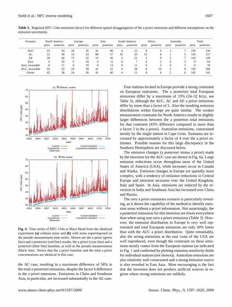
In the experiment without superimposed noise, theAFEAS/UNFCCC/CIESIN (AUC) emission field (Fig.3a)is almost perfectly reconstructed by the inversion (Fig.3b),with small differences occurring mostly in Asia where thereis a poor constraint by the measurements. Consequently, thea posteriori modeled mixing ratios are virtually identical tothe pseudo measurements, as shown for Mace Head (Fig.4a),

which features a Pearson correlation coefficient greater than0.999. This shows that the inversion algorithm has been setup correctly. However, this experiment is not very realisticas the pseudo measurement data were constructed with thesame transport model as was used for the inversion.

In the second experiment we mimicked measurementand model errors by superimposing onto the pseudo mea-surements normally distributed random noise with station-specific standard deviationσo (columnEb in Table2). Evenfor this case, the emission distribution in Europe – the con-tinent best constrained by the measurement data (see Fig.1)– is very well reconstructed (Fig.3c) and the total Europeanemission is only overestimated by 8%. Emissions in NorthAmerica, still reasonably well constrained by the measure-ments, are also fairly well reproduced with a total overesti-mate of 17%. However, the emissions in Asia are not welldetermined, with clearly deficient emission patterns and anoverall underestimate of 50% (a result of the regularizationconstraining the emissions towards zero). A few “ghost”sources appear at high northern latitudes, and emissions inthe Southern Hemisphere (not shown), especially in Africa,are also not well reconstructed: continental totals are in er-ror by more than a factor of 2. The pseudo measurementsat the stations are well reproduced by the inverse model, forinstance at Mace Head (Fig.4b), proving that it is the sparsedensity of measurement sites outside Europe that is mostproblematic for the inversion. Another experiment showedthat when pseudo measurements for the Hateruma station areadded, the emission distribution in eastern Asia is well recon-structed.

5.2 Sensitivity to the a priori emissions and their uncertain-ties

Next we evaluated the influence of the a priori emission in-formation on the inversion for HFC-134a. All measurementsfrom all stations (32400 values in total) were used, and westudied the following five scenarios:

1. In our standard method, theCIESIN (2005) pop-ulation map was used for distributing the UN-FCCC country emissions as well as the remainingAFEAS emissions without country-specific information(AFEAS/UNFCCC/CIESIN or AUC).

2. The AFEAS global emissions were distributed only ac-cording to population without using UNFCCC informa-tion (AFEAS/CIESIN or AC).

3. The EDGAR version 3.3 inventory for the year 1995(Olivier et al., 2001) was used for emission disaggrega-tion (AFEAS/EDGAR or AE).

4. A zero emission flux was assumed everywhere (Zero).



Fig. 3. Distribution of HFC-134a emissions taken from the a priori inventory based on AFEAS, UNFCCC and CIESIN data(a), reconstructedby inversion using the a priori model results as pseudo measurements(b), and reconstructed by inversion using the a priori model resultswith superimposed noise as pseudo measurements(c). Measurement sites are marked with black dots.

5. Using the AUC a priori, we allowed the inversion toalso produce non-zero emission fluxes over the oceans(Ocean).

For the zero emission flux and the AUC inversion we alsotested the influence of the assumed emission uncertainty. Forthat, we replaced our standard scenario (see Sect.4.5) witha globally constant uncertainty of 200% of the global meanemission flux.

The three a priori emission distributions (Fig.5a, b; ACdistribution not shown) are quite different from each other.Continental total emissions as reported in Table3 are a factorof 7 and 6 higher in Africa and Asia for the AC distribution

than for the AE distribution. The AC distribution does notreflect different degrees of industrialization and likely over-estimates emissions in less developed countries. Conversely,emissions in Europe are highest for the AE distribution, aresult of the rather outdated EDGAR inventory for the year1995 when HFC-134a emissions were still heavily weightedtowards North America and Europe. The AUC distribution(Fig. 5a) lies between the AE and AC distributions (Table3)and is probably most realistic.

The a posteriori HFC-134a emissions (Fig.5c, d, Table3)differ much less than the corresponding a priori emissions.Asian total emissions are more than doubled in the AE case,increased by 12% in the AUC case, and reduced by 35% in



Table 3. Regional HFC-134a emissions (kt/yr) for different spatial disaggregation of the a priori emissions and different assumptions on theemission uncertainty.

Scenario North America Europe Asia South America Africa Australia Totalprior posterior prior posterior prior posterior prior posterior prior posterior prior posterior prior posterior

AUC 65 43 24 26 41 46 4 22 8 6 2 7 145 156AC 12 30 14 24 88 57 10 25 15 6 1 5 145 157AE 49 40 73 32 15 36 3 21 2 9 2 7 145 149Zero 0 20 0 18 0 12 0 7 0 2 0 5 0 64

Zero, invariable 0 17 0 19 0 13 0 11 0 3 0 5 0 70AUC, invariable 65 52 24 28 41 51 4 28 8 10 2 8 145 184

Ocean 65 38 24 26 41 40 4 11 8 6 2 6 145 141

a) Without noise

35

40

45

50

55

60

65

70

0501 0504 0507 0510 0601 0604 0607 0610 0701 0704

HF

C-1

34a

(ppt

)

Date

A prioriA posteriori

Observed

A priori baselineA posteriori baseline

b) With noise

35

40

45

50

55

60

65

70

0501 0504 0507 0510 0601 0604 0607 0610 0701 0704

HF

C-1

34a

(ppt

)

Date


Observed


Fig. 4. Time series of HFC-134a at Mace Head from the idealizedexperiment(a) without noise and(b) with noise superimposed onthe pseudo measurement time series. Shown are the a priori (greenline) and a posteriori (red line) results, the a priori (cyan line) and aposteriori (blue line) baseline, as well as the pseudo measurements(black line). Notice that the a priori baseline and the total a prioriconcentrations are identical in this case.

the AC case, resulting in a maximum difference of 58% inthe total a posteriori emissions, despite the factor 6 differencein the a priori emissions. Emissions in China and SoutheastAsia, in particular, are increased substantially in the AE case.

Four stations located in Europe provide a strong constrainton European emissions. The a posteriori total Europeanemissions differ by a maximum of 33% (24–32 kt/yr, seeTable3), although the AUC, AC and AE a priori emissionsdiffer by more than a factor of 5. Also the resulting emissiondistributions within Europe are quite similar. The weakermeasurement constraint for North America results in slightlylarger differences between the a posteriori total emissionsfor that continent (43% difference compared to more thana factor 5 in the a priori). Australian emissions, constrainedmostly by the single station in Cape Grim, Tasmania are in-creased by approximately a factor of 4 over the a priori es-timates. Possible reasons for this large discrepancy in theSouthern Hemisphere are discussed below.

The emission changes (a posteriori minus a priori) madeby the inversion for the AUC case are shown in Fig.6a. Largeemission reductions occur throughout most of the UnitedStates of America (USA), while increases occur in Canadaand Alaska. Emission changes in Europe are spatially morecomplex, with a tendency of emission reductions in CentralEurope and emission increases over the United Kingdom,Italy and Spain. In Asia, emissions are reduced by the in-version in India and Southeast Asia but increased over Chinaand Russia.

The zero a priori emissions scenario is particularly reveal-ing, as it shows the capability of the method to identify emis-sion areas without a priori information. Not surprisingly, thea posteriori emissions for this inversion are lower everywherethan when using non-zero a priori emissions (Table3). How-ever, the emission distribution in Europe is very well rep-resented and total European emissions are only 30% lowerthan with the AUC a priori distribution. Quite remarkably,also the strong emissions at the east coast of the USA arewell reproduced, even though the constraint on these emis-sions mostly comes from the European stations (as indicatedin Fig.1 and confirmed by plotting emission sensitivity fieldsfor individual stations (not shown)). Australian emissions arealso relatively well constrained and a strong emission sourceis also revealed in East Asia. Most encouraging is the factthat the inversion does not produce artificial sources in re-gions where strong emissions are unlikely.



Fig. 5. Distribution of HFC-134a emissions for different a priori assumptions: a priori based on AFEAS/UNFCCC/CIESIN distribution(a), apriori based on EDGAR distribution(b), a posteriori using AFEAS/UNFCCC/CIESIN distribution as a priori(c), a posteriori using EDGARdistribution as a priori(d), a posteriori using zero emissions as a priori(e), a posteriori using AFEAS/UNFCCC/CIESIN distribution as apriori but allowing the inversion to also produce non-zero emissions over the oceans(f). Measurement sites are marked with black dots.

For the zero a priori emission scenario, we also tested howstrongly the inversion results depend on the assumed emis-sion uncertainties. In our standard inversion, the uncertaintyis 40% of the emission value in a grid box or 100% of theglobal mean emission flux, whichever is larger (for the zeroa priori emission scenario, the AUC uncertainties were used).As an alternative, we tested a spatially invariable uncertaintyof 200% of the global mean emission flux (Fig.5e). The con-tinental total a posteriori values for the two uncertainty sce-narios are almost identical (Table3), except for South Amer-ica where the masurement constraint is weak. The regionalemission distribution within the continents is also similar forboth scenarios but the patterns are smoother when using theinvariable emission uncertainty.

The influence of the emission uncertainty on the inversionresult was also tested for the AUC a priori. Using the spa-

tially invariable uncertainty leads to higher total emissions(Table 3). This is a result of the inversion not being ableto sufficiently reduce the source strengths in high-emissionregions. In high-emission grid cells, the invariable uncer-tainty is a too small fraction of the a priori source and, thus,the emissions are bound too tightly to their a priori values.The changes (a posteriori minus a priori) in the HFC-134aemission distribution are spatially more homogeneous whenusing the invariable emission uncertainty than when using avariable emission uncertainty (Fig.6). For instance, with theinvariable uncertainty, emissions are reduced by the inver-sion almost all over the USA. In contrast, with the variableuncertainty, large reductions are made at the east coast, witha more variable pattern of small increases and decreases else-where in the USA.



Fig. 6. Changes made by the inversion in the HFC-134a emissions (a posteriori minus a priori) for the AFEAS/UNFCCC/CIESIN a prioriwhen using a variable emission uncertainty(a) and when using a spatially invariable emission uncertainty(b).

Our default setup ignores boxes where more than 99% ofthe area is covered by water or ice. Allowing the inversion,using the AUC a priori emissions, to also produce emissionsthere, provides another check on the quality of the inversion.Although some spurious emissions can be found over theoceans in this case (Fig.5f), their source strengths are allvery low. In contrast, with the exception of South Americawhich is poorly constrained by measurement data, the emis-sions over the continents remain very similar to our defaultsetup (Table3).

5.3 Station-specific error statistics

Another way to look at the inversion results is to comparea priori and a posteriori errors at different stations for ourdefault inversion using the AUC a priori (Table2). At sta-tions that are not too far from source regions (Cape Grim,Mace Head, Trinidad Head, Hateruma) relative error reduc-tions (1− Eb/Ea in Table 2) between 25% and 55% areachieved. At more remote stations such as Zeppelin and Bar-bados, errors are reduced by around 15%. At Samoa, theerror reduction is marginal. This station is not influencedby sources on the time scale of 20 d included in our method(see Fig.1); thus it cannot make a contribution to the in-

version. The European mountain stations Jungfraujoch andMonte Cimone have the highest observed values and largesterrors, though the tail of the errors has already been clipped.In spite of this, only error reductions of 5% and, respectively,9%, are achieved. The reasons for this behaviour have al-ready been discussed in Sect.4.6.

At most stations, the variability and trend in the base-line explains a substantial fraction of the observed HFC-134avariations, shown as the squared Pearson correlation coeffi-cientr2

bl between the a priori baseline and the observed con-centrations in Table2 (results using the a posteriori baselineare nearly identical).r2

bl is highest for remote stations (e.g.,r2bl = 0.94 for Zeppelin) where events with transport from

source regions on the time scale of 20 d are rare, intermediateat stations not too far from source regions (e.g.,r2

bl=0.44 forMace Head) where short-term variability is large, and lowestat the mountain stations where short-term variability domi-nates (e.g.,r2

bl = 0.03 for Jungfraujoch).

Variability in the excess of the observed values over thebaseline is mainly the result of transport events. A correlationanalysis of the excess with the simulated emission contribu-tions from the last 20 d reveals to what extent these events arecaptured by the model. This was done using both the a priori



(r2ea in Table2) and a posteriori model results (r2

eb in Table2).This analysis confirms the previous finding that the transportmodel has no explanatory power at the remote station Samoa(r2

eb=0.03). The model also performs poorly at the mountainstation Jungfraujoch (r2

eb=0.04), partly because of some “in-curable” large errors, which were used with a reduced weightin the inversion but are included in the calculation of thecorrelation coefficients. The situation is a little better at theMonte Cimone mountain site (r2

eb=0.16) where the inversionalso results in an improvement of the correlation. The modelperforms much better at the other sites. At Mace Head, it caneven explain 74% of the observed short-term variance.

The correlations between observations and model results(i.e., baseline plus 20 d source contributions,r2

a and r2b in

Table2) are high at all flatland stations (74–95% of the vari-ance in the observations explained by the a posteriori modelresults). Only at the mountain stations Jungfraujoch (11%)and Monte Cimone (39%), the observations cannot be ex-plained well.

Figure 7 shows two examples for time series of the ob-servations and inversion results for the stations Mace Headand Trinidad Head where substantial error reductions couldbe achieved by the inversion. At both stations, the a prioriconcentrations are reduced, quite substantially so in the caseof Trinidad Head where also the baseline is shifted upwardto compensate for the reduced source contributions from the20 d transport. At Mace Head, even the a priori simulationcaptures the majority of the transport episodes, and the a pos-teriori results show excellent agreement with the measure-ments.

5.4 Tests with a subset of the data

To investigate how sensitive the inversion result is to theavailability of data from different stations, we repeated theinversion using the AUC a priori information but in one casewe removed all data from the Mace Head station and in an-other case we removed all data from the mountain stationsJungfraujoch and Monte Cimone. The results are comparedin Fig. 8 to the inversion using the full data set by showingthe increments to the a priori caused by the inversion. Sta-tions outside Europe were kept in the inversion but have asmall influence on the results for Europe. The total Euro-pean emissions are very similar in all three a posteriori cases(26.4, 28.0 and 24.4 kt/yr for the default inversion, the casewithout Mace Head data and the case without Jungfraujochand Monte Cimone data) and are all higher than in the a pri-ori AUC inventory (24.2 kt/yr). This shows that the measure-ment data from the different stations are quite consistent witheach other in constraining the European total emissions de-spite the modeling problems at the mountain stations. A sim-ilar experiment done with the AE a priori, which has a threetimes larger European total emission than the AUC a prioriyielded similar a posteriori results, showing that the smalldifferences in the a posteriori total European source strength

a) Mace Head

35

40

45

50

55

60

65

70

0501 0504 0507 0510 0601 0604 0607 0610 0701 0704

HF

C-1

34a

(ppt

)

Date


Observed


-15-10-5 0 5

10 15

HF

C-1

34a

erro

r (p

pt)

b) Trinidad Head

40

45

50

55

60

0504 0507 0510 0601 0604 0607 0610 0701 0704

HF

C-1

34a

(ppt

)

Date


Observed


-20-15-10-5 0 5

10 15 20

HF

C-1

34a

erro

r (p

pt)

Fig. 7. Time series of HFC-134a at Mace Head(a) and TrinidadHead (b) obtained with the standard inversion setup using theAFEAS/UNFCCC/CIESIN a priori. Shown are the a priori (greenline) and a posteriori (red line) results, the a priori (cyan line) anda posteriori (blue line) baseline, as well as the observations (blackline). The lower panels show the observed and simulated HFC-134amixing ratios, the upper panels the corresponding model errors.

are not the result of binding the inversions too tightly to the apriori. In fact, substantial corrections to the a priori occur onthe regional scale. These corrections are broadly consistentbetween the three different inversions shown in Fig.8, result-ing in increases over the United Kingdom, Southern Europeand Eastern Europe, and in small regions in Central Europe,and substantial decreases over large parts of Central Europe,Scandinavia and around Moscow. This encouraging resultsuggests that even the data from the mountain stations arevaluable in guiding the inversion on the regional scale. How-ever, notice also that the removal of data from Mace Headhas a stronger impact on the inversion than the removal ofboth Jungfraujoch and Monte Cimone data, a consequenceof the lower model skill for the mountain stations. Thereare also some inconsistencies between the inversion results



a) Mace Head removed b) Jungfraujoch, Mt. Cimone removed

c) all stations d) AFEAS/UNFCCC/CIESIN, a priori

Fig. 8. Sensitivity of the a HFC-134a inversion result to the removal of data. Shown are the changes (a posteriori minus a priori) of theHFC-134a emissions when using all stations except Mace Head(a), all stations except Jungfraujoch and Monte Cimone(b), all stations(d),as well as the a priori emission distribution(d). The lower left color bar refers to all difference plots (panels a-c), whereas the lower rightcolor bar only refers to panel d. Measurement stations are marked with black dots.

but they are mostly restricted to individual grid boxes. Forinstance, emissions are increased over Madrid when MaceHead data are removed but decreased in the other cases, andthe relatively large changes made to the emissions in CentralEurope deviate somewhat in location between the differentexperiments.

Another inversion experiment was done using only datafrom Jungfraujoch, the station with the poorest model per-formance. Also data from stations outside Europe were re-moved. The corrections to the a priori were much smallerin this case but the patterns were broadly consistent with theother results, showing for example emission increases in theUnited Kingdom and Eastern Europe.

In summary, our sensitivity experiments show that the in-version algorithm is working properly as intended and pro-duces consistent results both for idealized and realistic se-tups. In the following, we will apply the algorithm to deter-mine the emissions of HFC-134a, HFC-152a and HCFC-22.While our inversion algorithm at present does not yield for-mal uncertainties of the a posteriori emission fluxes, from therange of results obtained in the sensitivity experiments wesubjectively estimate that they are accurate to within betterthan 20% for Europe and to within 30% for other regions wellconstrained by measurements (North America, large parts ofAsia). For smaller regions (e.g., individual small countries),

errors may be larger. Future work should consider both a bet-ter characterization of the a priori uncertainties of the emis-sion fluxes, as well as an error propagation to yield corre-sponding uncertainties also of the a posteriori results.

6 HFC inversion results

6.1 HFC-134a

HFC-134a inversion results for our reference case using theAFEAS/UNFCCC/CIESIN a priori were presented in detailalready in Sect.5 and are further discussed here. To facilitateinterpretation, we show results from inversions done sepa-rately for the years 2005 and 2006, and we also report totalsfor some selected countries that are big enough to be resolvedby our model grid. The results must be interpreted cautiouslywhere large emissions occur near borders and, thus, attribu-tion of the gridded emissions to a country is somewhat prob-lematic (e.g., Canada, Germany). Both for the a priori as wellas for the a posteriori results, total HFC-134a emissions in-crease from 2005 to 2006 (see Table4). However, while the apriori emissions increase everywhere (no UNFCCC country-specific information was available for years after 2005 whenthis work was done), the a posteriori emissions increase inEurope (mostly in Eastern Europe) and Asia (especially in



Table 4. Regional emissions (kt/yr) for the years 2005 and 2006 and the total period with available data (January 2005 to March 2007)for HFC-134a, HFC-152a, and HCFC-22. Results for South America and Africa are not reported because of insufficient constraints bymeasurement data. Global totals are less affected by errors for South America and Africa and are shown.

Species North America Europe Asia Australia Totalprior posterior prior posterior prior posterior prior posterior prior posterior

HFC-134a, all data 65 43 24 26 41 46 2 7 145 156HFC-134a, 2005 61 41 23 24 38 42 2 5 136 130HFC-134a, 2006 68 38 25 27 42 44 2 5 150 140HFC-152a, all data 11.5 15.6 3.3 4.0 7.0 10.9 0.0 0.6 23.8 37.0HFC-152a, 2005 11.2 12.3 3.2 3.5 6.8 9.6 0.0 0.4 23.0 28.9HFC-152a, 2006 11.8 15.1 3.3 3.9 7.1 9.8 0.0 0.2 24.3 33.4HCFC-22, all data 62 80 13 24 244 149 1 12 346 333HCFC-22, 2005 60 53 12 24 234 133 1 9 332 251HCFC-22, 2006 64 62 13 23 249 146 1 7 354 300

China) but decrease in North America. The increase in Eu-rope is a continuation of the upward trend seen also in theUNFCCC data until 2005, while the decrease in North Amer-ica (due to a decrease in the USA, see Table5) could indicatea trend reversal. UNFCCC data for the USA and Canada in-deed show a leveling-off between 2004 and 2005 of the previ-ously positive emission trend. Our a posteriori emissions forthe USA of 35 kt/yr (28 kt/yr) for 2005 (2006) are further-more only 61% (50%) of the UNFCCC value. They agreevery well with the even somewhat lower values ofMillet etal. (2009) who obtained 27 (range of 12–39) kt/yr using air-craft measurement data from the years 2004 and 2006 and ahalocarbon-carbon monoxide ratio method to determine theUSA emissions.

For Europe, the a posteriori emissions are somewhathigher than the industry-based a priori emissions and suggesta 13% increase from 2005 to 2006. In contrast,O’Dohertyet al. (2004) found for several periods (latest period 2000–2002) that emissions derived from simulations with theNAME model and an inverse algorithm were about a factor 2smaller than the industry-based value. If both model-derivedvalues are correct, this could indicate delayed emissions dueto lower leakage rates of HFC-134a, which is mainly used inrefrigeration and air-conditioning. More likely, however, thea posteriori emissions fromO’Doherty et al.(2004) are toolow, especially since their European emissions are only 12%of their reported global emissions, which seems low. Further-more,Reimann et al.(2004) derived much higher Europeanemissions of 23.6 kt/yr for the same period (2000–2002), al-most identical to our estimate for 2005 and 2006. Still, our aposteriori source distribution in Europe is quite similar to thatshown byO’Doherty et al.(2004), lending confidence to bothapproaches. The source distribution is, however, very differ-ent from the potential source regions shown byReimann etal. (2008) andMaione et al.(2008) based on statistical anal-yses of back trajectories and HFC-134a data from the moun-tain sites Jungfraujoch and Monte Cimone. We attribute this

Table 5. HFC-134a emissions (kt/yr) from UNFCCC for the year2005 and a posteriori inversion results for selected countries for theyears 2005 and 2006. Estimated uncertainties of the a posteriorivalues are generally 20–30% but may be somewhat larger for coun-tries with substantial emissions close to borders with other countries(e.g., Germany). Uncertainties in the relative changes from the year2005 to 2006, however, are likely to be only about 20% since thegeometry of the observation network has not changed between theyears.

Country UNFCCC 2005 2006

USA 56.9 34.8 28.1Canada 2.2 3.3 3.5France 5.1 5.6 5.1Germany 4.0 2.0 2.3Ireland 0.2 0.3 0.3Italy 1.8 2.4 3.9Poland 1.7 0.9 1.4Spain 1.6 2.1 2.1United Kingdom – 1.9 1.8Russia – 6.4 5.6China – 9.8 11.9Japan 3.5 5.3 4.0Australia 1.9 4.9 4.5

to artifacts in their trajectory statistics, which are likely tooccur especially in regions not frequently passed by trajecto-ries.

While many western European countries (e.g., France, Ire-land, Spain, United Kingdom) had constant or slightly de-creasing emissions from 2005 to 2006, emissions in somesouthern (e.g., Italy) and eastern (e.g., Poland) Europeancountries increased (Table5). In general, there is relativelygood agreement between UNFCCC reported emissions andour a posteriori emissions for the year 2005 for most Euro-pean countries.



For Asia, between 2005 and 2006 we find an increase ofemissions in China and a decrease in Japan (Table5). Ac-cording to UNFCCC, emissions in Japan peaked in 2003 anddecreased by 25% until 2005. Our results confirm decreasingemissions in Japan but the 2005 total is 50% higher than theUNFCCC total. For China, we obtain annual emissions of9.8 and 11.9 kt/yr for the years 2005 and 2006, respectively,substantially more than the 3.9 kt/yr reported byYokouchi etal. (2006) for the period May 2004–May 2005, which was de-rived using Hateruma HFC-134a to carbon monoxide ratiosand a – likely too low – estimate of Chinese carbon monoxideemissions. Our results indicate that China is now a substan-tial emitter of HFC-134a with a 20% growth in emissionsfrom 2005 to 2006. For Australia, our a posteriori emis-sions for 2005 and 2006 are about a factor 2.5 larger thanthe industry-based a priori (see Table4 and discussion belowfor possible explanation).

6.2 HFC-152a

HFC-152a has an estimated atmospheric lifetime of 1.55 yr(Greally et al., 2007) and is used predominately in foam-blowing and aerosol spray applications (Ashford et al.,2004b). For HFC-152a, the a priori emission data werecalculated slightly differently than for HFC-134a. As noglobal emission data from AFEAS are available, we usedprojections fromAshford et al.(2004b) for 2005–2007 di-rectly (i.e., without adjustment to AFEAS emissions). Fur-thermore, UNFCCC country total emissions are available forfewer countries than for HFC-134a. Where available, weused this information. Data for the USA – the largest emit-ter of HFC-152a, according toAshford et al.(2004b) – aremissing for confidentiality reasons. A distribution of emis-sions according to the world population distribution woulddefinitely lead to an underestimation of HFC-152a emissionsin the USA (about 1 kt/yr). Inversion experiments done withsuch a low a priori value for the USA lead to a more thanfour-fold increase of emissions in the USA and unrealisti-cally high emissions in border regions of Canada, as theinversion algorithm is trying to compensate for far too lowUSA emissions. To bring the a priori estimate closer to thesuspected real emissions, we therefore assumed an annualemission of 10 kt/yr in the USA, about 40% of the globalemissions.

The inversion results in a substantial increase (55% for thewhole period) of global HFC-152a emissions relative to thea priori emission fromAshford et al.(2004b) (see Table4and Fig.9). The relative increase is larger for the full periodthan for the individual years because the stronger constraintfrom the larger measurement data set can drive the a poste-riori solution further away from the a priori emissions. Thiseffect is especially evident in this case of HFC-152a wherethe a priori emissions are systematically too low in all conti-nents. Since the solution is bound towards a too low a priori,it is likely that our inversion results (particularly for the indi-

Table 6. HFC-152a emissions (t/yr) from UNFCCC for the year2005 and a posteriori inversion results for selected countries for theyears 2005 and 2006.

Country UNFCCC 2005 2006

USA – 10 100 12 509Canada 918 1470 1592France 314 626 479Germany 781 434 459Ireland 7 15 18Italy – 259 388Poland 24 20 22Spain 170 351 175United Kingdom – 88 76Russia – 1185 1123China – 3162 3655Japan 1217 1532 1267Australia - 357 221

vidual years) are actually a lower estimate of the true globalsource strength.

Greally et al. (2007) calculated the global HFC-152asource from AGAGE data and an inverse 12-box model.They found a more rapid (and accelerating) increase of HFC-152a emissions than reported byAshford et al.(2004b) fromindustry data. For the year 2004,Greally et al.(2007) re-ported a source strength of 28.5 kt, compared to only 21.9 ktfrom Ashford et al.(2004b). Our results confirm this strongersource and also indicate that emissions have grown morerapidly from 2005 to 2006 than the industry-based estimateof Ashford et al.(2004b).

The inversion increases the emissions in all continents (seeTable4 and Fig.9), even in North America, where high a pri-ori emissions of 10 kt/yr for the USA alone were used.Milletet al.(2009), based on their aircraft data, reported somewhatlower emissions for the USA (7.6 kt/yr with a range of 5.7–9.7 kt/yr) than what we have obtained (10.1 and 12.5 kt/yrfor 2005 and 2006, respectively). However, most of theirdata was from the year 2004 and, given the strong trend, canstill be considered in good agreement. The smallest increasesoccur in Europe where many countries have reported theiremissions to UNFCCC and our a priori estimate should bemost accurate. Most of these increases occur in SouthernEurope (see Fig.9c), especially in Italy and in some regionsof Spain. European emissions derived by the inversion in-creased from 2005 to 2006, whereas emissions reported bythe European Union decreased from 2003 to 2005. Increas-ing emissions higher than reported by the EU countries werealready found byGreally et al.(2007) using inversions basedon another LPDM andReimann et al.(2004) using measure-ment data from Jungfraujoch. There is some agreement inregional emission patterns in Europe between our results andthose reported byGreally et al.(2007), Maione et al.(2008)andReimann et al.(2008).



Fig. 9. A priori (a), a posteriori(b) and a posteriori minus a priori(c) emissions of HFC-152a using the full measurement data set. Measure-ment stations are marked with black dots.



The inversion increases the emissions in Asia by about50%, with a doubling of the a priori emissions in China (seeFig. 9) and a 16% increase from 2005 to 2006 (see Table6).Our estimated Chinese HFC-152a emissions of 3.2-3.7 kt/yrare in good agreement with the 4.3 kt/yr recently reported byYokouchi et al.(2006) for the period May 2004 to May 2005.

HFC-152a emissions in Australia are relatively small (ca.200-600 t/yr, depending on period) but significantly largerthan the 5-10 t/yr reported byGreally et al.(2007). Figure10shows time series of HFC-152a for the Cape Grim station inTasmania. HFC-152a concentrations are very low and themeasurements show a lot of variability, which partly appearto be associated with instrumental noise and probably the ad-vection of air masses with variable background but withoutrecent emission input, which makes the inversion difficult.However, some of the longer-lasting variations require an in-crease by an order of magnitude of the low a priori emissionfor Australia (28 t/yr) in order to be captured by the model.While it is possible that the a priori emissions for Australiaare too low, such a large increase is not consistent with HFCconsumption data for Australia. Thus, the large a posterioriemissions in Australia point towards a problem of our inver-sion setup. One problem is that Australia is constrained onlyby a single station, Cape Grim, which is located to the southof the emission sources. At the same time, the halocarbonbackground concentrations increase with latitude and, in par-ticular, are much higher in the northern than in the SouthernHemisphere. Thus, air masses transported across Australiasouthward to the station would tend to be associated with el-evated concentrations, even without the additional emissioninput from Australia. In such a situation, the inversion al-gorithm would attempt to attribute the observed concentra-tion increase to emissions in Australia. This effect could po-tentially overshadow actual emissions in Australia especiallyfor substances where Australian emissions are very low com-pared to those in the Northern Hemisphere. Given the presentgeometry of the observation networks, our algorithm is ob-viously not sensitive enough to quantify the relatively smallemission source in Australia. The problem may be exacer-bated by the point-like nature of emission sources in Aus-tralia (e.g., those in Melbourne), which are not resolved byour inversion grid.

6.3 HCFC-22

HCFC-22 is the most abundant of the hydrochlorofluorocar-bons measured in the atmosphere and has a lifetime of about12 yr (O’Doherty et al., 2004). It is used in refrigeration,as a foam-blowing agent, and it is also used for the produc-tion of fluoropolymers (McCulloch et al., 2006). Regard-ing our a priori emissions, we used global annual HCFC-22emissions fromAshford et al.(2004b). Country totals forthe annual consumption of HCFCs (not only HCFC-22) inthe year 2006, expressed in terms of the ozone-depletion po-tential, are available from the United Nations Environment

1.8 2

2.2 2.4 2.6 2.8

3 3.2 3.4

0501 0504 0507 0510 0601 0604 0607 0610 0701 0704

HF

C-1

52a

(ppt

)

Date


Observed


-0.3-0.2-0.1

0 0.1 0.2 0.3

HF

C-1

52a

erro

r (p

pt)

Fig. 10.Time series of HFC-152a in Tasmania. Shown are the a pri-ori (green line) and a posteriori (red line) results, the a priori (cyanline) and a posteriori (blue line) baseline, as well as the observa-tions (black line). The lower panels show the observed and simu-lated HFC-152a mixing ratios, the upper panels the correspondingmodel errors.

Programme (http://ozone.unep.org/), see alsoUNEP(2005).We identified the 22 countries with the largest HCFC con-sumption which together are responsible for nearly 92% ofreported global emissions. China alone contributed almost50% to the global HCFC consumption in 2006, in agree-ment with the report byMcCulloch et al.(2006) of rapidlygrowing HCFC-22 production in China. Country totals weredistributed according to the CIESIN population distributionwithin the respective countries, and remaining global emis-sions were also distributed according to population. HCFC-22 data from Jungfraujoch were not used because of a knowncontamination problem.

The global emissions after the inversion (Fig.11 and Ta-ble4) are reduced slightly (by 4%, 25% and 15% for the fullperiod, the year 2005 and the year 2006, respectively) com-pared to the a priori total emission. However, there are largeregional differences between the a priori and the a posterioriemissions. For instance, emissions in Europe are doubled,emissions in Asia are reduced by about 40% (largely becauseof reductions in China) and emissions in Australia are in-creased by an order of magnitude. The emission increasein Europe can be explained by a time lag between HCFC-22 consumption as contained in the UNEP statistics and theactual time of emission occurrence, since reported HCFC-22 consumption in Europe is dropping rapidly (a hint of adecrease from 2005 to 2006 is seen in the inversion results).Such a time lag is plausible since HCFC-22 (a refrigerant andfoam-blowing agent) is not released to the atmosphere imme-diately when used. A time lag between reported consumptionand emission can also explain the lower a posteriori HCFC-22 emissions in Asia since emissions in China are growingrapidly. The large increase for Australia is thought to be anartifact of the method, as discussed above for HFC-152a.


http://ozone.unep.org/


Fig. 11. A priori (a), a posteriori(b) and a posteriori minus a priori(c) emissions of HCFC-22 using the full measurement data set.Measurement stations are marked with black dots.



Table 7. HCFC-22 emissions (t/yr) used as the a priori and a poste-riori inversion results for selected countries for the years 2005 and2006. Only total HCFC consumption data are available from UNEP,and no country-specific information was available for the EuropeanUnion, so data in the ”UNEP/a priori” column are based on ourdisaggregated gridded data.

Country UNEP/a priori 2005 2006

USA 44 603 32 864 31 940Canada 5300 7170 4922France 873 4527 3397Germany 879 601 768Ireland 56 253 254Italy 655 2821 2783Poland 482 252 220Spain 463 1884 1045United Kingdom 725 1898 1813Russia 7592 10 339 10 159China 16 6119 59 759 70 650Japan 6966 10 181 7785Australia 1027 8925 7264

For the USA (33 and 32 kt/yr for 2005 and 2006), there isagain a good agreement with the study ofMillet et al. (2009)who obtained 46 (21–69) kt/yr based on aircraft data. In Eu-rope, the inversion increases the emissions most strongly inwestern and Southern Europe (e.g., a factor of 4–5 in France,Italy and Spain, see Table7), whereas emissions in someregions in Eastern Europe are even decreased (e.g., a fac-tor 2 decrease in Poland). In Asia, the dominant feature isa large reduction by the inversion of emissions in China,whereas emissions in Japan are increased. Regarding thechange from 2005 to 2006, the inversion produces a 18%emission increase for China and a 24% decrease for Japan,in line with the large reported changes of HCFC consump-tion in these two countries. Again, this indicates a lag of afew years between the year of reported HCFC-22 consump-tion and the time of actual emission. Substantial emissionincreases are also made by the inversion in Central Amer-ica, which could point towards an underreporting of HCFCconsumption there.

7 Discussion and conclusions

We have further developed the analytical inversion methodof Seibert(2000, 2001) to determine the regional and globalemissions of long-lived GHGs from concentration measure-ments. The method is based on 20 d backward simulationsfrom a number of measurement stations using a Lagrangianparticle dispersion model. It objectively determines a time-varying baseline concentration for each station and uses theobserved and modeled enhancements over the baseline to im-prove an a priori emission distribution. The method con-

tains a detailed treatment of the uncertainties in the model-measurement comparison as well as in the a priori emissionfield. A propagation of these uncertainties to the a posteri-ori emission fluxes is left to future development, which willalso require an improved knowledge of the a priori emissionerrors.

We applied the method to HFC-134a, HFC-152a andHCFC-22 measurements obtained at eight stations of theAGAGE and SOGE networks and a Japanese station. Un-fortunately, most of the nine stations are not ideally placedfor determining regional emission fluxes. Some (e.g., Amer-ican Samoa) are too remote and are not influenced by emis-sions on the time scale considered in our model calculations(20 d). As already noted byMahowald et al.(1997), locatingthe observing stations closer to the source regions would im-prove the ability of inversion methods to deduce source infor-mation. At the mountain stations (Jungfraujoch, Monte Ci-mone), the model has big difficulties in reproducing the ob-served concentration variability because of the complex lo-cal meteorology, close-by emission sources, and the episodictransport of pollutants from these local sources. While thedata from these stations still help constraining the emissions,the data value for the inversion would increase substantiallyif the stations were moved to topographically less complexlocations while, however, still staying outside the proximityof strong sources. Finally, the global distribution of the sta-tions is not satisfactory. While at least three stations providedirect information on European emissions, not a single sta-tion provides a good constraint on the emissions in Africaand large parts of South America (Fig.1). Also emissionsin India, Indonesia and Northern Australia are not well con-strained by the data.

For the siting of stations in the future, we recommend thatthe sources in every continent should be constrained by atleast two stations. The first station should be placed down-wind of the continental emissions in the main continentalpollution outflow, other stations should be placed as far awayfrom the first station as possible to “view” the major sourceregions from a different angle. This would help the inver-sion in separating the emission strengths of different regionswithin the continent. Ideally, the stations should be locatedeither near the coastline or better even on small islands justdownwind of the shoreline in areas not strongly influencedby emission sources within about 50–100 km of the station.Mace Head, Trinidad Head and Hateruma are relatively wellplaced according to the above criteria but they are not in themain pollution outflow pathway and, thus, sample the con-tinental emissions somewhat too infrequently. A new obser-vatory that is currently being built at Birkenes in southernNorway will hopefully fulfill all the above criteria and, thus,holds the promise of delivering an extremely valuable dataset to better constrain regional emissions in Europe. Mosturgent, however, would be the addition of stations in tropicalareas where constraints are currently missing almost entirely(see Fig.1): probably on the Maldives to constrain emissions



from India, at the Pacific and Atlantic coasts of NorthernSouth America to constrain emissions in South America, atthe Cape Verde islands to constrain emissions in Africa, orin Northeastern Australia to constrain emissions in North-ern Australia and Indonesia. Before deciding on a location,backward model calculations should be done specifically forcandidate sites to find out which options would yield the bestoverall improvement of the global emission sensitivity dis-tribution (Fig.1). In this context, it could be interesting tomake use of backward transport calculations carried out rou-tinely by the Comprehensive Nuclear Test Ban Treaty Organ-isation (CTBTO/PrepCom) for its global network of radionu-clide monitoring stations (Wotawa et al., 2003; Becker et al.,2007). This network is also interesting because at these sitesthe necessary infrastructure is already available.

When fed with pseudo observations generated by thetransport model, our inversion method can reconstruct theemission distribution used for generating the model resultsalmost perfectly (see Fig.3). Even when noise is superim-posed on the data, the emission reconstruction is nearly per-fect in areas that are well constrained by the pseudo obser-vations. However, in areas not so well constrained (muchof the Southern Hemisphere), the result is tied more closelytowards the a priori emission field.

Using real HFC-134a data, we have explored the sensitiv-ity of the method to changes in the a priori emission field andits uncertainties. In well constrained regions (Europe, partsof North America and Asia), the a posteriori emission fieldsare quite close to each other; however, large differences canoccur in the Southern Hemisphere (Fig.5 and Table3). Evenwhen using no a priori information (zero a priori emissions),the major emission areas in Europe, North America and east-ern Asia can be identified. While the source strengths aretoo low in this case, due to the regularization constrainingthe emissions towards zero, the bias for the well-constrainedregions is only about−40%. The method is also relativelyrobust against the removal of data from individual stations.

One particular problem was identified for Australia, whereemissions are constrained by a single station, Cape Grim.This station is located south of the major emission sources,whereas the halocarbon background in the Southern Hemi-sphere increases towards the north. Thus, southward trans-port across Australia would be associated with elevated con-centrations, even if Australian emissions were zero. At thesame time, actual emissions in Australia are so small thattheir signal can easily be overshadowed by the advection of avarying background, which is erroneously attributed to Aus-tralian emissions by the inversion algorithm. This points to-wards a possible improvement of our inversion algorithm.Instead of specifying a baseline for each individual station,the baseline nodes could be defined for a few latitude bands.The instantaneous baseline at a particular station could thenbe calculated by considering the correct initial condition atthe beginning of each 20 d particle trajectory. That way, thebaseline at a station would depend on the “origin” of an air

mass. In the example for Australia, this would mean a higherbaseline for transport from the north.

In our inversions for HFC-134a, HFC-152a and HCFC-22,we found that our global a posteriori emissions increased forall three species from 2005 to 2006. The largest increases(21%, 16%, 18%, respectively) from 2005 to 2006 werefound for China, in line with the relatively strong halocar-bons emissions in Eastern Asia reported elsewhere (Palmeret al., 2003). In contrast, changes in the emissions in NorthAmerica and Europe were modest from 2005 to 2006. ForEurope, the a posteriori emissions of HFC-134a and HFC-152a were slightly higher than the a priori emissions reportedto the UNFCCC. For HCFC-22, the a posteriori emissions forEurope were substantially (by almost a factor 2) higher thanthe a priori emissions, which were based on HCFC consump-tion data reported to UNEP. Combined with the reportedstrongly decreasing HCFC consumption in Europe, this sug-gests a substantial time lag between the reported timing of theHCFC-22 consumption and the actual timing of the HCFC-22 emission. Similarly, in China where HCFC consumptionis increasing rapidly according to the UNEP data, our a pos-teriori emissions are only about 40% of the estimated annualHCFC-22 consumption used for the a priori emissions, re-vealing a substantial storage of HCFC-22 and potential forfuture emission in China.

The basic methodology described in this paper can ofcourse be applied to many other substances that have suffi-ciently long lifetimes to consider them stable during a periodon the order of 20 d.

Acknowledgements.We appreciate the comments from tworeviewers on the ACPD version of this paper, which helped shapingthis final version. We thank Met.no and ECMWF for access to theECMWF data. P. Seibert acknowledges the support of the Fondszur Forderung der wissenschaftlichen Forschung (FWF, grant17924) and the EU-FP6 Network of Excellence ACCENT.

Edited by: L. Carpenter

References

AFEAS (Alternative Fluorocarbons Environmental AcceptabilityStudy): Production, sales, and emission data for 2005: AFEAS,Arlington, VA , USA, (seewww.afeas.org), 2007.

Ashford, P., Clodic, D., McCulloch, A., and Kuijpers, L.: Emis-sion profiles from the foam and refrigeration sectors comparisonwith amtospheric concentrations. Part 1: Methodology and data,Intern. J. Refrigeration, 27, 687–700, 2004a.

Ashford, P., Clodic, D., McCulloch, A., and Kuijpers, L.: Emis-sion profiles from the foam and refrigeration sectors comparisonwith amtospheric concentrations. Part 2: Results and discussion,Intern. J. Refrigeration, 27, 701–716, 2004b.

Becker, A., Wotawaa, G., De Geer, L.-E., Seibert, P., Draxler, R. R.,et al.: Global backtracking of anthropogenic radionuclides bymeans of a receptor oriented ensemble dispersion modelling sys-tem in support of Nuclear-Test-Ban Treaty verification, Atmos.Environ., 41, 4520–4534, 2007.


www.afeas.org


Chen, Y.-H. and Prinn, R. G.: Estimation of atmosphericmethane emissions between 1996–2001 using a 3D globalchemical transport model, J. Geophys. Res., 111, D10307,doi:10.1029/2005JD006058, 2006.

Chipperfield, M. and V. Fioletov (Lead Authors): Global Ozone:Past and Present, Chapter 3 in Scientific Assessment of OzoneDepletion 2006, Global Ozone Research and Monitoring Project-Report No. 50, 3.1–3.58, WMO, Geneva, Switzerland, 2007.

Center for International Earth Science Information Network(CIESIN): Gridded Population of the World: Future Esti-mates, Socioeconomic Data and Applications Center (SEDAC),Columbia University, Palisades, NY, USA, 2005. Available athttp://sedac.ciesin.columbia.edu/gpw(downloaded on 22 April2008).

Clerbaux, C. and D. Cunnold (lead Authors): Long-Lived Com-pounds, Chapter 1 in Scientific Assessment of Ozone Depletion2006, Global Ozone Research and Monitoring Project-ReportNo. 50, 1.1–1.63, WMO, Geneva, Switzerland, 2007.

Damoah, R., Spichtinger, N., Forster, C., James, P., Mattis, I.,Wandinger, U., Beirle, S., and Stohl, A.: Around the world in17 days – hemispheric-scale transport of forest fire smoke fromRussia in May 2003, Atmos. Chem. Phys., 4, 1311–1321, 2004,http://www.atmos-chem-phys.net/4/1311/2004/.

Dunse, B., Steele, P., Wilson, S., Fraser, P., and Krummel, P.: Tracegas emissions from Melbourne Australia, based on AGAGE ob-servations at Cape Grim, Tasmania, 1995–2000, Atmos. Envi-ron., 39, 6334–6344, 2005.

ECMWF, White, P. W. (ed.): IFS Documentation, ECMWF, Read-ing, UK, 2002.

Eckhardt, S., Breivik, K., Man, S., and Stohl, A.: Record high peaksin PCB concentrations in the Arctic atmosphere due to long-range transport of biomass burning emissions, Atmos. Chem.Phys., 7, 4527–4536, 2007,http://www.atmos-chem-phys.net/7/4527/2007/.

Eckhardt, S., Prata, A. J., Seibert, P., Stebel, K., and Stohl, A.: Es-timation of the vertical profile of sulfur dioxide injection into theatmosphere by a volcanic eruption using satellite column mea-surements and inverse transport modeling, Atmos. Chem. Phys.,8, 3881–3897, 2008,http://www.atmos-chem-phys.net/8/3881/2008/.

Emanuel, K. A., andZivkovic-Rothman, M.: Development andevaluation of a convection scheme for use in climate models, J.Atmos. Sci., 56, 1766–1782, 1999.

Enomoto, T., Yokouchi, Y., Izumi, K., and Inagaki, T.: Develop-ment of an analytical method for atmospheric halocarbons andits application to airborne observation, J. Jpn. Soc. Atmos. Envi-ron., 40, 1–8, 2005 (in Japanese).

Enting, I.: Inverse Problems in Atmospheric Constituent Transport,Cambridge University Press, Cambridge, UK, 392 pp., 2002.

Forster, C., Stohl, A., and Seibert, P.: Parameterization of convec-tive transport in a Lagrangian particle dispersion model and itsevaluation, J. Appl. Meteor. Clim., 46, 403–422, 2007.

Forster, P., Ramaswamy, V., Artaxo, P., Berntsen, T., Betts, R., Fa-hey, D. W., Haywood, J., Lean, J., Lowe, D. C., Myhre, G.,Nganga, J., Prinn, R., Raga, G., Schulz, M., and Van Dorland,R.: Changes in Atmospheric Constituents and in Radiative Forc-ing, in: Climate Change 2007: The Physical Science Basis. Con-tribution of Working Group I to the Fourth Assessment Reportof the Intergovernmental Panel on Climate Change, edited by:

Solomon, S., Qin, D., Manning, M., Chen, Z., Marquis, M., Av-eryt, K. B., Tignor, M., and Miller, H. L., Cambridge UniversityPress, Cambridge, UK and New York, NY, USA, 2007.

Greally, B. R., Manning, A. J., Reimann, S., McCulloch, A., Huang,J., et al.: Observations of 1,1-difluoroethane (HFC-152a) atAGAGE and SOGE monitoring stations in 1994-2004 and de-rived global and regional emission estimates, J. Geophys. Res.,112, D06308, 10.1029/2006JD007527, 2007.

Hartley, D. and Prinn, R.: Feasibility of determining surfaceemissions of trace gases using an inverse method in a three-dimensional chemical transport model, J. Geophys. Res., 98,5183–5197, 1993.

Kasibhatla, P., Heimann, M., Rayner, P., Mahowald, N., Prinn, R.,and Hartley, D. (eds.): Inverse Methods in Global Biogeochem-ical Cycles, American Geophysical Union (AGU) GeophysicalMonograph Series, 114, 324 pp., 2000.

Mahowald, N. M., Prinn, R. G., and Rasch, P. J.: Deducing CCl3Femissions using an inverse method and chemical transport mod-els with assimilated winds, J. Geophys. Res., 102, 28153–28168,1997.

Maione, M., Arduini, J., Mangani, G., and Geniali, A.: Evaluationof an automatic sampling gas chromatographic-mass spectromet-ric instrument for continuous monitoring of trace anthropogenicgases, Int. J. Environ. Anal. Chem., 84, 241–253, 2004.

Maione, M., Giostra, U., Arduini, J., Belfiore, L., Furlani, F., Ge-niali, A., Mangania, G., Vollmer, M. K., and Reimann, S.: Local-ization of source regions of selected hydrofluorocarbons combin-ing data collected at two European mountain stations, Sci. TotalEnviron., 391, 232–240, 2008.

Manning, A. J., Ryall, D. B., Derwent, R. G., Simmonds, P. G.,and O’Doherty, S.: Estimating European emissions of ozone-depleting and greenhouse gases using observations and a mod-eling back-attribution technique, J. Geophys. Res., 108, 4405,2003.

McCulloch, A., Midgley, P. M., and Ashford, P.: Releases of re-frigerant gases (CFC-12, HCFC-22 and HFC-134a) to the atmo-sphere, Atmos. Environ., 37, 889–902, 2003.

McCulloch, A., Midgley, P. M., and Lindley, A. A.: Recent changesin the production and global atmospheric emissions of chlorodi-fluoromethane (HCFC-22), Atmos. Environ., 40, 936–942, 2006.

Menke, W.: Geophysical Data Analysis: Discrete Inverse Theory,Academic Press, Orlando, USA, 260 pp., 1984.

Miller, B. R., Weiss, R. F., Salameh, P. K., Tanhua, T., Greally, B.R., Muhle, J., and Simmonds, P. G.: Medusa: A sample precon-centration and GC/MS detector system for in situ measurementsof atmospheric trace halocarbons, hydrocarbons, and sulfurcompounds, Anal. Chem., 1536–1545, doi:10.1021/ac702084k,2008.

Millet, D. B., E. L. Atlas, D. R. Blake, N. J. Blake, G. S. Diskin,et al. (2009): Halocarbon Emissions from the United States andMexico and Their Global Warming Potential, Environ. Sci. Tech-nol., 43, 1055–1060, 2009.

Mulquiney, J. E., Taylor, J. A., Jakeman, A. J., Norton, J. P., andPrinn, R. G.: A new inverse method for trace gas flux estimation:2. Application to tropospheric CFCl3 fluxes, J. Geophys. Res.,103, 1429–1442, 1998.

O’Doherty, S., Cunnold, D. M., Manning, A., Miller, B. R., Wang,R. H. J., et al.: Rapid growth of hydrofluorocarbon 134a andhydrochlorofluorocarbons 141b, 142b, and 22 from Advanced


http://sedac.ciesin.columbia.edu/gpw

http://www.atmos-chem-phys.net/4/1311/2004/




Global Atmospheric Gases Experiment (AGAGE) observationsat Cape Grim, Tasmania, and Mace Head, Ireland, J. Geophys.Res., 109, D06310, doi:10.1029/2003JD004277, 2004.

Olivier, J. G. J. and Berdowski, J. J. M.: Global emissions sourcesand sinks, edited by: Berdowski, J., Guicherit, R. and Heij, B.J. (eds.) in: The Climate System, 33–78, A. A. Balkema Pub-lishers/Swets & Zeitlinger Publishers, Lisse, The Netherlands,ISBN: 90-5809-255-0.

Palmer, P. I., Jacob, D. J., Mickley, L. J., Blake, D. R., Sachse, G.W., et al.: Eastern Asian emissions of anthropogenic halocarbonsdeduced from aircraft concentration data, J. Geophys. Res., 108,4753, doi:10.1029/2003JD003591, 2003.

Prinn, R. G., Weiss, R. F., Fraser, P. J., Simmonds, P. G., Cun-nold, D. M., et al: A history of chemically and radiatively impor-tant gases in air deduced from ALE/GAGE/AGAGE, J. Geophys.Res., 105, 17751–17792, 2000.

Reimann, S., Schaub, D., Stemmler, K., Folini, D., Hill, M.,Hofer, P., Buchmann, B., Simmonds, P. G., Greally, B. R., andO’Doherty, S.: Halogenated greenhouse gases at the Swiss highalpine site of Jungfraujoch (3580 m asl): Continuous measure-ments and their use for regional European source allocation, J.Geophys. Res., 109, D05307, doi:10.1029/2003JD003923, 2004.

Reimann, S., Vollmer, M. K., Folini, D., Steinbacher, M., Hill,M., Buchmann, B., Zander, R., and Mahieu, E.: Observationsof long-lived anthropogenic halocarbons at the high-Alpine siteof Jungfraujoch (Switzerland) for assessment of trends and Eu-ropean sources, Sci. Total Environ., 391, 223–231, 2008.

Seibert, P.: Inverse modelling of sulfur emissions in Europe basedon trajectories, in: Inverse Methods in Global BiogeochemicalCycles, edited by: Kasibhatla, P., Heimann, M., Rayner, P., Ma-howald, N., Prinn, R. G., and Hartley, D. E., 147–154, Geophys-ical Monograph 114, American Geophysical Union, ISBN:0-87590-097-6, 2000.

Seibert, P.: Inverse modelling with a Lagrangian particle dispersionmodel: application to point releases over limited time intervals,In: Air Pollution Modeling and its Application XIV, edited by:Schiermeier, F. A. and Gryning, S.-E., Kluwer Academic Publ.,381–389, 2001.

Seibert, P. and Frank, A.: Source-receptor matrix calculation with aLagrangian particle dispersion model in backward mode, Atmos.Chem. Phys., 4, 51–63, 2004,http://www.atmos-chem-phys.net/4/51/2004/.

Seibert, P. and Skomorowski, P.: Untersuchung der orographis-chen Besonderheiten der Probennahmestellen Schauinsland undFreiburg und deren Auswirkungen auf die Genauigkeit von ad-jungierten atmospharischen Ausbreitungsrechnungen, Schriften-reihe Reaktorsicherheit und Strahlenschutz, BMU-2008-713,194 pp.,http://www.bmu.de/41875, 2008.

Simmonds, P. G., Odoherty, S., Nickless, G., Sturrock, G. A.,Swaby, R., Knight, P., Ricketts, J., Woffendin, G., and Smith, R.:Automated Gas-Chromatograph Mass-Spectrometer for RoutineAtmospheric Field-Measurements of the Cfc Replacement Com-pounds, the Hydrofluorocarbons and Hydrochlorofluorocarbons,Anal. Chem., 67, 717–723, 1995.

Stohl, A., Hittenberger, M., and Wotawa, G.: Validation of theLagrangian particle dispersion model FLEXPART against largescale tracer experiment data, Atmos. Environ., 32, 4245–4264,1998.

Stohl, A. and Thomson, D. J.: A density correction for Lagrangianparticle dispersion models, Bound.-Lay. Meteorol., 90, 155–167,1999.

Stohl, A., S. Eckhardt, C. Forster, P. James, and N.Spichtinger: On the pathways and timescales of interconti-nental air pollution transport, J. Geophys. Res., 107, 4684,doi:10.1029/2001JD001396, 2002.

Stohl, A., Forster, C. Eckhardt, S., Spichtinger, N., Huntrieser, H.,Heland, J., Schlager, H., Wilhelm, S., Arnold, F., and Cooper, O.:A backward modeling study of intercontinental pollution trans-port using aircraft measurements, J. Geophys. Res., 108, 4370,doi:10.1029/2002JD002862, 2003.

Stohl, A., Forster, C., Frank, A., Seibert, P., and Wotawa, G.: Tech-nical note: The Lagrangian particle dispersion model FLEX-PART version 6.2., Atmos. Chem. Phys., 5, 2461–2474, 2005,http://www.atmos-chem-phys.net/5/2461/2005/.

Stohl, A., Berg, T., Burkhart, J. F., Fjæraa, A. M., Forster, et al.:Arctic smoke – record high air pollution levels in the EuropeanArctic due to agricultural fires in Eastern Europe, Atmos. Chem.Phys., 7, 511–534, 2007,http://www.atmos-chem-phys.net/7/511/2007/.

Technology and Economic Assessment Panel: Supplement to theIPCC/TEAP report, United Nations Environment Programme,Nairobi, ISBN: 92-807-2733-8, 2005.

United Nations Environment Programme (UNEP): Production andConsumption of Ozone Depleting Substances under the MontrealProtocol 1986-2004, Ozone Secretariat, UNEP, Nairobi, Kenya,75 pp., 2005.

Wotawa, G., De Geer, L.-E., Denier, P., Kalinowski, M., Toivonen,H., D’Amours, R., Desiato, F., Issartel, J.-P., Langer, M., Seibert,P., Frank, A., Sloan, C., and Yamazawa, H.: Atmospheric trans-port modelling in support of CTBT verification – overview andbasic concepts, Atmos. Environ., 37, 1565–1573, 2003.

Yokouchi, Y., Taguchi, S., Saito, T., Tohjima, Y., Tanimoto, H., andMukai, H.: High-frequency measurements of HFCs at a remotesite in east Asia and their implications for Chinese emissions,Geophys. Res. Lett., 33, L21814, doi:10.1029/2006GL026403,2006.



http://www.bmu.de/41875



an analytical inversion method for determining regional ... · (e.g. manning et al., 2003;...

Documents