an analysis of the surf method - image processing - · pdf filean analysis of the surf method...
TRANSCRIPT
Published in Image Processing On Line on 2015–07–20.Submitted on 2013–02–12, accepted on 2015–05–30.ISSN 2105–1232 c© 2015 IPOL & the authors CC–BY–NC–SAThis article is available online with supplementary materials,software, datasets and online demo athttp://dx.doi.org/10.5201/ipol.2015.69
2015/06/16
v0.5.1
IPOL
article
class
An Analysis of the SURF Method
Edouard Oyallon1, Julien Rabin2
1 ENS, Departement Informatique, France ([email protected])2 University of Caen, GREYC - ENSICAEN, France ([email protected])
Abstract
The SURF method (Speeded Up Robust Features) is a fast and robust algorithm for local,similarity invariant representation and comparison of images. Similarly to many other localdescriptor-based approaches, interest points of a given image are defined as salient features froma scale-invariant representation. Such a multiple-scale analysis is provided by the convolutionof the initial image with discrete kernels at several scales (box filters). The second step consistsin building orientation invariant descriptors, by using local gradient statistics (intensity andorientation). The main interest of the SURF approach lies in its fast computation of operatorsusing box filters, thus enabling real-time applications such as tracking and object recognition.The SURF framework described in this paper is based on the PhD thesis of H. Bay [ETHZurich, 2009], and more specifically on the paper co-written by H. Bay, A. Ess, T. Tuytelaarsand L. Van Gool [Computer Vision and Image Understanding, 110 (2008), pp. 346–359]. Animplementation is proposed and used to illustrate the approach for image matching. A shortcomparison with a state-of-the-art approach is also presented, the SIFT algorithm of D. Lowe[International Journal of Computer Vision, 60 (2004), pp. 91–110], with which SURF shares alot in common.
Source Code
The source code and the online demo are accessible at the IPOL web page of this article1. Theproposed implementation of the SURF algorithm is written in C++ ISO/ANSI. It performsfeatures extraction from digital images and provides local correspondences for a pair of images.An epipolar geometric consistency checking may additionally be used to discard mismatcheswhen considering two pictures from the same scene. This optional post-processing uses theORSA algorithm by B. Stival and L. Moisan [International Journal of Computer Vision, 57(2004), pp. 201–218].
Keywords: SURF; SIFT; image comparison; local descriptors; feature detection; featurematching
1http://dx.doi.org/10.5201/ipol.2015.69
Edouard Oyallon, Julien Rabin, An Analysis of the SURF Method, Image Processing On Line, 5 (2015), pp. 176–218.http://dx.doi.org/10.5201/ipol.2015.69

An Analysis of the SURF Method
1 Introduction
1.1 Context, Motivation and Previous Work
Over the last decade, the most successful algorithms to address various computer vision problems havebeen based on local, affine-invariant descriptions of images. The targeted applications encompass,but are not limited to, image stitching and registration, image matching and comparison, indexationand classification, depth estimation and 3-D reconstruction. Like many image processing approaches,a popular and efficient methodology is to extract and compare local patches from different images.However, in order to design fast algorithms and obtain compact and locally invariant representations,some selection criteria and normalization procedures are required. A sparse representation of theimage is also necessary to avoid extensive patch-wise comparisons that would be computationallyexpensive. The main challenges are thus to keep most salient features from images (such as corners,blobs or edges) and then to build a local description of these features which is invariant to variousperturbations, such as noisy measurements, photometric changes, or geometric transformation.
Such problems have been addressed since the early years of computer vision, resulting in a veryprolific literature. Without being exhaustive, one may first mention the famous Stephen-Harriscorner detector [9], and the seminal work of Lindeberg on multi-scale feature detection (see e.g. [12]).Secondly, invariant local image description from multi-scale analysis is a more recent topic: SIFTdescriptors [15] –from which SURF [2] is largely inspired– are similarity invariant descriptors of animage that are also robust to noise and photometric change. Some algorithms extend this frameworkto fully affine transformation invariance [18, 28], and dense representation [26].
The main interest of the SURF approach [2] studied in this paper is its fast approximation of theSIFT method. It has been shown to share the same robustness and invariance while being faster tocompute.
1.2 Outline and Algorithm Overview
The SURF algorithm is in itself based on two consecutive steps (feature detection and description)that are described in Sections 4 and 5. The last step is specific to the application targeted. In thispaper, we chose image matching as an illustration (Sections 5.4 and 6).
Multi-scale analysis Similarly to many other approaches, such as the SIFT method [15], thedetection of features in SURF relies on a scale-space representation, combined with first and secondorder differential operators. The originality of the SURF algorithm (Speeded Up Robust Features) isthat these operations are speeded up by the use of box filters techniques (see e.g. [25], [27]) that aredescribed in Section 2. For this reason, we will use the term box-space to distinguish it from the usualGaussian scale-space. While the Gaussian scale space is obtained by convolution of the initial imageswith Gaussian kernels, the discrete box-space is also obtained by convolving the original image withbox filters at various scales. A comparison between these two scale-spaces is proposed in Section 3.
Feature detection During the detection step, the local maxima in the box-space of the “determi-nant of Hessian” operator are used to select interest point candidates (Section 4). These candidatesare then validated if the response is above a given threshold. Both the scale and location of thesecandidates are then refined using quadratic fitting. Typically, a few hundred interest points aredetected in a megapixel image.
Feature description The purpose of the next step described in Section 5 is to build a descriptorof the neighborhood of each point of interest that is invariant to view-point changes. Thanks to
177
Edouard Oyallon, Julien Rabin
multi-scale analysis, the selection of these points in the box-space provides scale and translationinvariance. To achieve rotation invariance, a dominant orientation is defined by considering the localgradient orientation distribution, estimated from Haar wavelets. Using a spatial localization grid, a64-dimensional descriptor is then built, based on first order statistics of Haar wavelets coefficients.
Feature matching Finally, when considering the image matching task (e.g. for image registra-tion, object detection, or image indexation), the local descriptors from several images are matched.Exhaustive comparison is performed by computing the Euclidean distance between all potentialmatching pairs. A nearest-neighbor distance-ratio matching criterion is then used to reduce mis-matches, combined with an optional RANSAC-based technique [21, 20] for geometric consistencychecking.
Outline The rest of the paper is structured as follows
– Section 2 SURF multi-scale representation based on box filters;
– Section 3 Comparison with linear scale space analysis;
– Section 4 Interest points detection;
– Section 5 Invariant descriptor construction and comparison;
– Section 6 Experimental validation and comparison with other approaches.
1.3 Notations
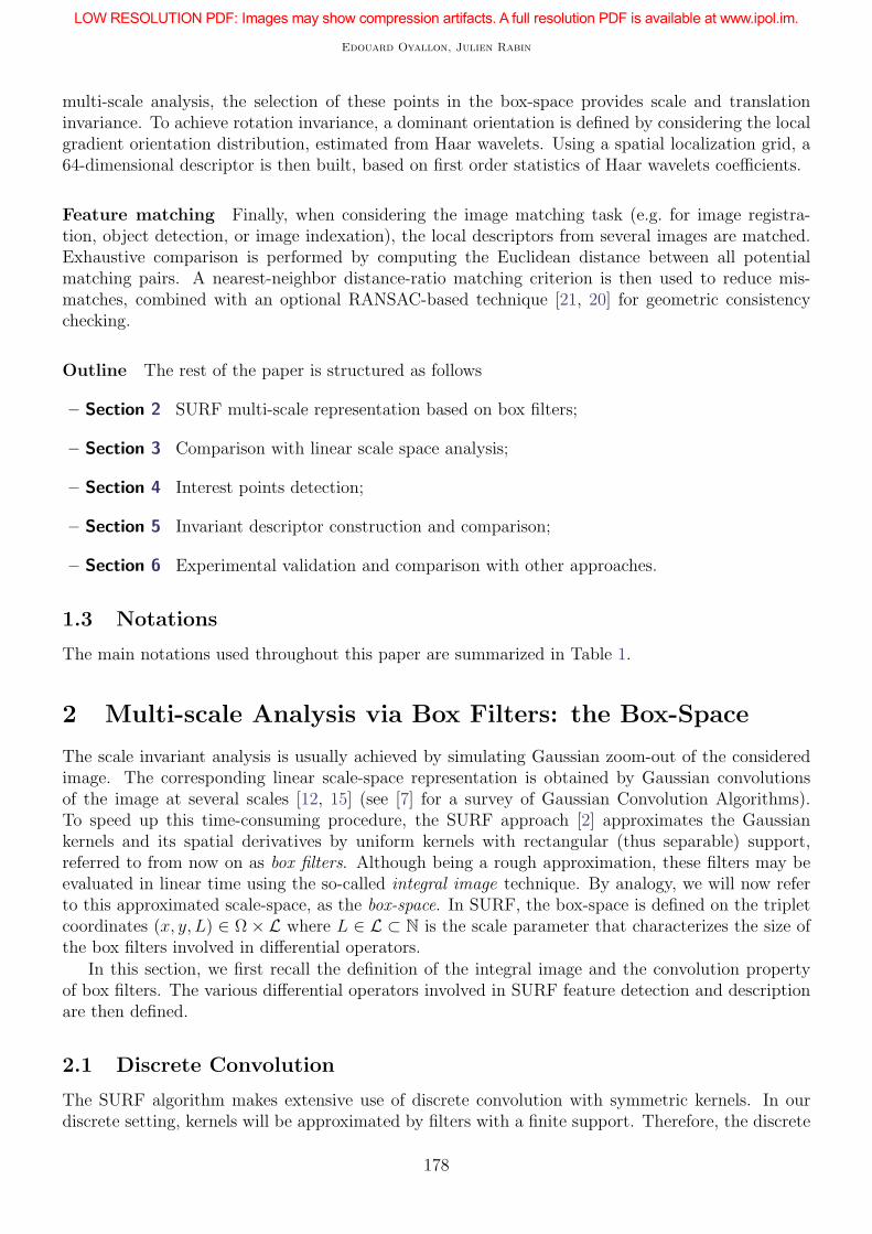
The main notations used throughout this paper are summarized in Table 1.
2 Multi-scale Analysis via Box Filters: the Box-Space
The scale invariant analysis is usually achieved by simulating Gaussian zoom-out of the consideredimage. The corresponding linear scale-space representation is obtained by Gaussian convolutionsof the image at several scales [12, 15] (see [7] for a survey of Gaussian Convolution Algorithms).To speed up this time-consuming procedure, the SURF approach [2] approximates the Gaussiankernels and its spatial derivatives by uniform kernels with rectangular (thus separable) support,referred to from now on as box filters. Although being a rough approximation, these filters may beevaluated in linear time using the so-called integral image technique. By analogy, we will now referto this approximated scale-space, as the box-space. In SURF, the box-space is defined on the tripletcoordinates (x, y, L) ∈ Ω× L where L ∈ L ⊂ N is the scale parameter that characterizes the size ofthe box filters involved in differential operators.
In this section, we first recall the definition of the integral image and the convolution propertyof box filters. The various differential operators involved in SURF feature detection and descriptionare then defined.
2.1 Discrete Convolution
The SURF algorithm makes extensive use of discrete convolution with symmetric kernels. In ourdiscrete setting, kernels will be approximated by filters with a finite support. Therefore, the discrete
178
An Analysis of the SURF Method
Symbol Description Definition
u image on a continuous domain u : R2 7→ R
u Discretized image u : (x, y) ∈ Ω ⊂ Z2 7→ [0, 256[⊂ R
U Integral image Formula (1)
δ(a,b) Discrete Dirac δ(a,b)(x, y) =
1 if (x, y) = (a, b)
0 otherwise
∗ Convolution/Discrete convolution Section 2.1
DLx ,D
Ly First order box filters, at scale L Section 2.3.1, Equation (6) & (7)
DLxx,D
Lyy,D
Lxy Second order box filters, at scale L Section 2.3.2, Equation (10) & (11)
DoHL Determinant of Hessian, at scale L Section 4.1, Equation (24)
∆L Laplacian, at scale L Section 4.3, Equation (28)
Dx, Dxy, ... First and second order derivative operator
DoHσScale normalized Determinant of
Hessian at scale σSection 3.3.3, Equation (22)
∆σ Scale normalized Laplacian, at scale σ Section 3.3.3, Equation (23)
J., .K Discrete interval Jn,mK = n, n+ 1, . . . ,M,∀n < m ∈ N
⌊·⌉ Round Closest integer
XT Matrix transposition XTi,j = Xj,i
1X Indicator function 1X(x) =
1 if x ∈ X
0 otherwise
Br(X) Ball of radius r, centered in X at Ω See Section 5
‖·‖ Norm See Sections 3.3 , 4.1, 5.3, and 5.4
∠ · Oriented angle with canonical vector(1, 0)T , ∠ : R2 7→ [−π, π) See Section 5.2
Rθ Rotation Matrix in R2 See Formula (41)
Table 1: List of main symbols and operators.
179
Edouard Oyallon, Julien Rabin
→ →
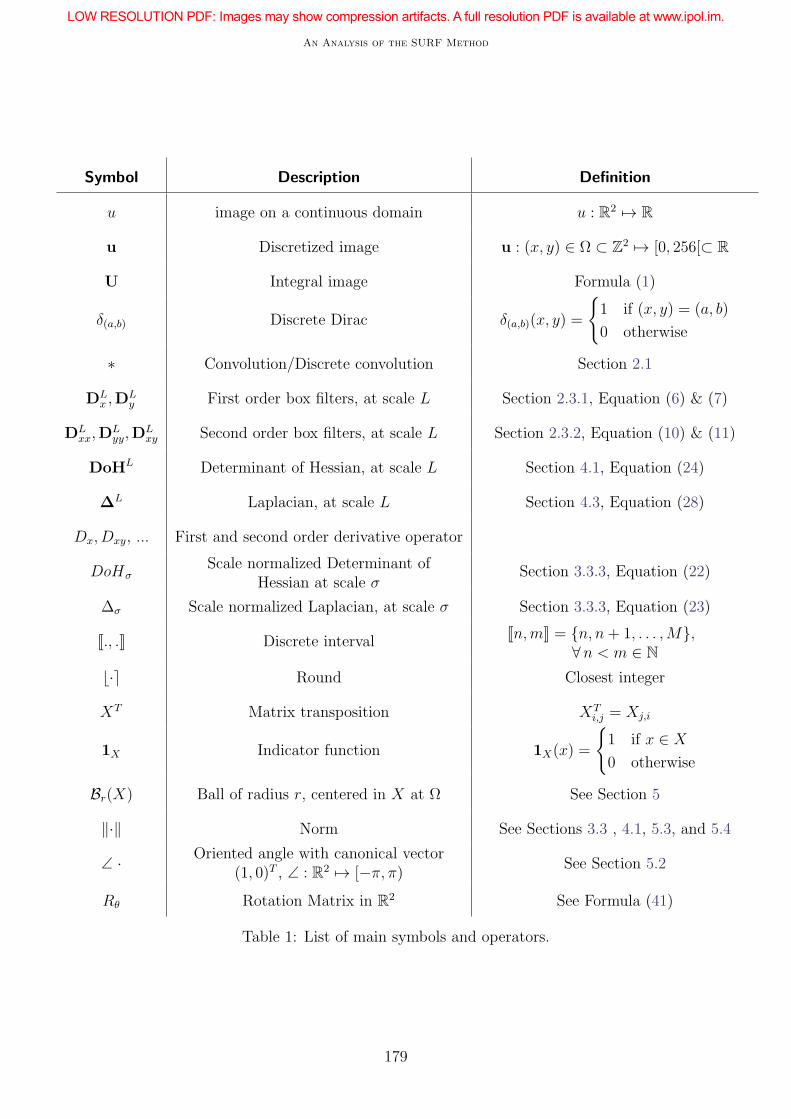
Figure 1: Illustration of preprocessing to create symmetric border condition. (Left) original lenaimage; (Middle) conversion in gray values and image dynamic stretching; (Right) extension by sym-metrization.
convolution of a discrete function f : Z2 → R with a discrete filter g : Ω ⊂ Z2 → R with finite
support Ω is defined as
∀ (x, y) ∈ Z2, (f ∗ g)(x, y) :=
∑
(i,j)∈Ωf(x− i, y − j) g(i, j). (1)
Borders condition In practice, an image f is known on a finite domain. As a result, bound-ary conditions must be handled properly in order to lessen visual artifacts at the borders. In ourimplementation, this difficulty is tackled through the use of symmetric boundary conditions. Thesymmetrization of the input image is performed with respect to the first and last rows and columns,so that there is no duplication of pixels at the boundaries. More precisely, the original image issymmetrically extended on each side using the largest box filter size (see Figure 1) before computingthe integral image.
Image sub-sampling Contrary to many other multi-scale approaches that build Gaussian pyramidcombined with dyadic sub-sampling to save computation time, the integral image technique detailedhereafter permits fast evaluation of differential operators at different scales without sub-sampling.However, sub-sampling may still be used to speed-up feature detection at larger scales (which isperformed in the proposed implementation).
Image interpolation Note that, as suggested in [1, 2] to improve the accuracy of the SURFmethod, the input image may be over-sampled and interpolated using a bilinear scheme. However,in this article we chose not to implement it.
Image dynamic The last preprocessing consists in a simple affine stretching of the image dynamicto J0, 255K.
180
An Analysis of the SURF Method
2.2 Integral Image and Box Filters
Let u be the processed digital image defined over the pixel grid Ω = J0, N−1K×J0,M−1K, where Mand N are positive integers. In the following, we only consider quantized gray valued images (takingvalues in the range J0, 255K), which is the simplest way to achieve robustness to color modifications,such as a white balance correction.
The integral image of u for (x, y) ∈ Ω is
U(x, y) :=∑
0≤i≤x
∑
0≤j≤y
u(i, j). (2)
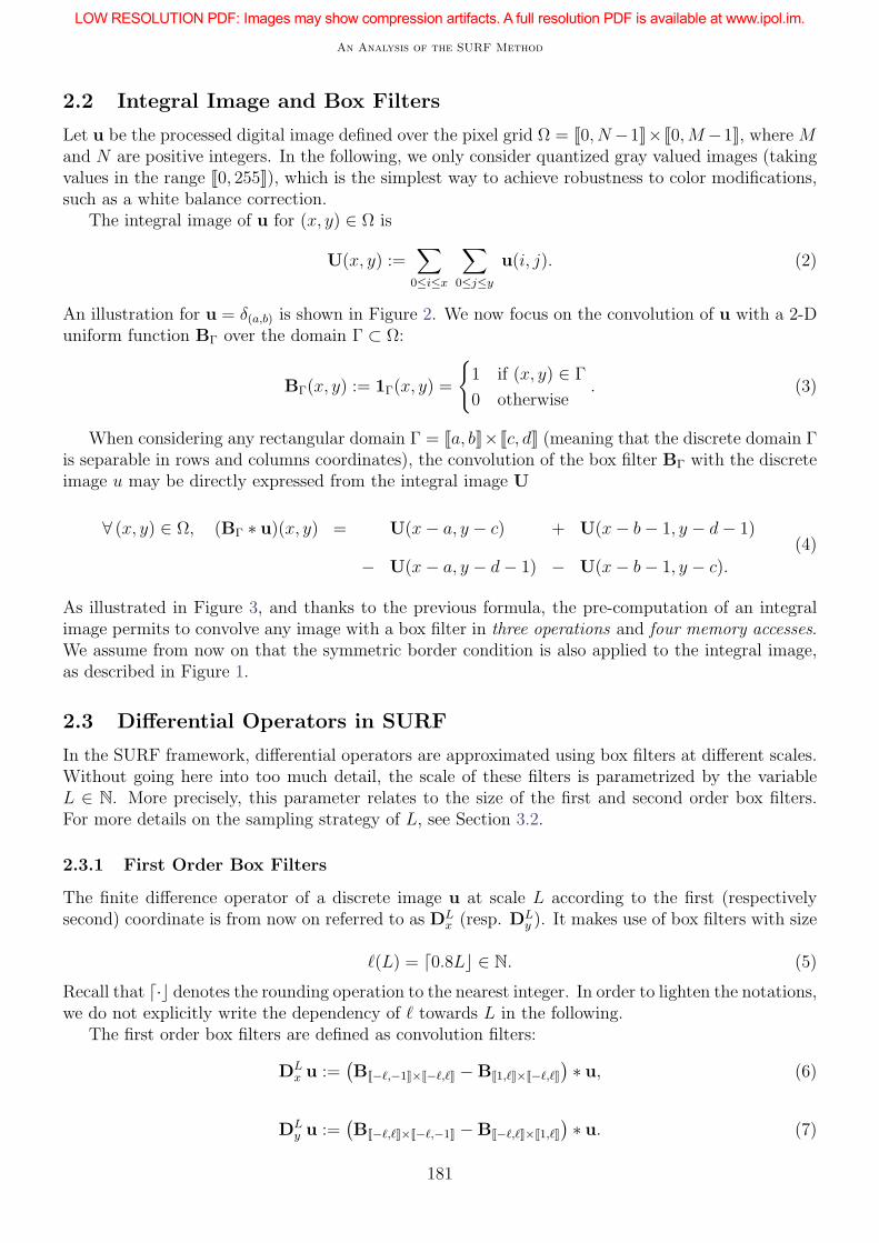
An illustration for u = δ(a,b) is shown in Figure 2. We now focus on the convolution of u with a 2-Duniform function BΓ over the domain Γ ⊂ Ω:
BΓ(x, y) := 1Γ(x, y) =
1 if (x, y) ∈ Γ
0 otherwise. (3)
When considering any rectangular domain Γ = Ja, bK×Jc, dK (meaning that the discrete domain Γis separable in rows and columns coordinates), the convolution of the box filter BΓ with the discreteimage u may be directly expressed from the integral image U
∀ (x, y) ∈ Ω, (BΓ ∗ u)(x, y) = + U(x− a, y − c) + U(x− b− 1, y − d− 1)
− U(x− a, y − d− 1) − U(x− b− 1, y − c).
(4)
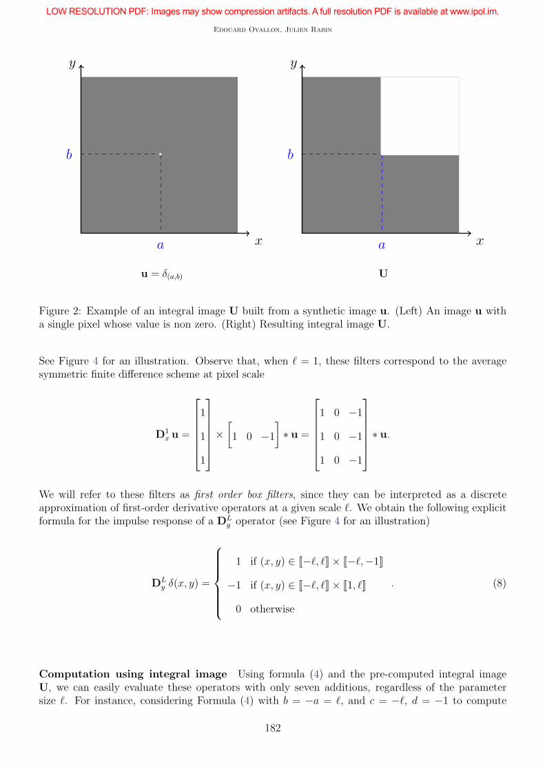
As illustrated in Figure 3, and thanks to the previous formula, the pre-computation of an integralimage permits to convolve any image with a box filter in three operations and four memory accesses.We assume from now on that the symmetric border condition is also applied to the integral image,as described in Figure 1.
2.3 Differential Operators in SURF
In the SURF framework, differential operators are approximated using box filters at different scales.Without going here into too much detail, the scale of these filters is parametrized by the variableL ∈ N. More precisely, this parameter relates to the size of the first and second order box filters.For more details on the sampling strategy of L, see Section 3.2.
2.3.1 First Order Box Filters
The finite difference operator of a discrete image u at scale L according to the first (respectivelysecond) coordinate is from now on referred to as DL
x (resp. DLy ). It makes use of box filters with size
ℓ(L) = ⌈0.8L⌋ ∈ N. (5)
Recall that ⌈·⌋ denotes the rounding operation to the nearest integer. In order to lighten the notations,we do not explicitly write the dependency of ℓ towards L in the following.
The first order box filters are defined as convolution filters:
DLx u :=
(
BJ−ℓ,−1K×J−ℓ,ℓK −BJ1,ℓK×J−ℓ,ℓK
)
∗ u, (6)
DLy u :=
(
BJ−ℓ,ℓK×J−ℓ,−1K −BJ−ℓ,ℓK×J1,ℓK
)
∗ u. (7)
181
Edouard Oyallon, Julien Rabin
y
xa
b
y
xa
b
u = δ(a,b) U
Figure 2: Example of an integral image U built from a synthetic image u. (Left) An image u witha single pixel whose value is non zero. (Right) Resulting integral image U.
See Figure 4 for an illustration. Observe that, when ℓ = 1, these filters correspond to the averagesymmetric finite difference scheme at pixel scale
D1x u =
1
1
1
×[
1 0 −1]
∗ u =
1 0 −1
1 0 −1
1 0 −1
∗ u.
We will refer to these filters as first order box filters, since they can be interpreted as a discreteapproximation of first-order derivative operators at a given scale ℓ. We obtain the following explicitformula for the impulse response of a DL
y operator (see Figure 4 for an illustration)
DLy δ(x, y) =
1 if (x, y) ∈ J−ℓ, ℓK× J−ℓ,−1K
−1 if (x, y) ∈ J−ℓ, ℓK× J1, ℓK
0 otherwise
. (8)
Computation using integral image Using formula (4) and the pre-computed integral imageU, we can easily evaluate these operators with only seven additions, regardless of the parametersize ℓ. For instance, considering Formula (4) with b = −a = ℓ, and c = −ℓ, d = −1 to compute
182
An Analysis of the SURF Method
y
xx− b− 1 x− a
y − d− 1
y − c +1
+1 -1
-1
Figure 3: Computation of the discrete convolution with box filter on a rectangular domain usingintegral image. Only 3 operations and 4 memory accesses are required per pixel, according toFormula (4).
BJ−ℓ,ℓK×J−ℓ,−1K, followed by c = +1, d = ℓ for BJ−ℓ,ℓK×J1,ℓK, we get
∀ (x, y) ∈ Ω, DLy u(x, y) = + U(x+ ℓ, y + ℓ) + U(x− ℓ− 1, y)
− U(x+ ℓ, y) − U(x− ℓ− 1, y + ℓ)
− U(x+ ℓ, y − 1) − U(x− ℓ− 1, y − ℓ− 1)
+ U(x+ ℓ, y − ℓ− 1) + U(x− ℓ− 1, y − 1).
(9)
Remark The original authors of SURF [2] simply claim to use Haar wavelets, but without givingany implementation details about the actual form of the kernels. Given this indeterminacy, weadopted anti-symmetric kernels (see Figure 4) because they do not introduce translation shifts.
2.3.2 Second Order Box Filters
In SURF, the multi-scale second order differential operators are again defined with box filters. Thesefilters are parametrized by a scale variable L ∈ N, which takes odd values. By analogy with secondorder difference schemes, the second order operators DL
xx and DLyy at scale L are defined as (see
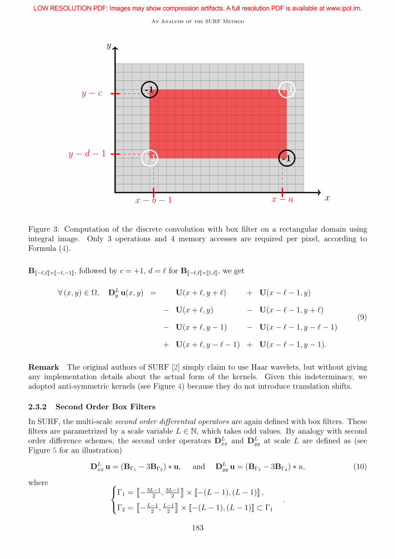
Figure 5 for an illustration)
DLxx u = (BΓ1 − 3BΓ2) ∗ u, and DL
yy u = (BΓ3 − 3BΓ4) ∗ u, (10)
where
Γ1 =q−3L−1
2, 3L−1
2
y× J−(L− 1), (L− 1)K ,
Γ2 =q−L−1
2, L−1
2
y× J−(L− 1), (L− 1)K ⊂ Γ1
.
183

Edouard Oyallon, Julien Rabin
ℓ
2ℓ+ 10
0
+1 −1
Figure 4: Illustration of the first order box filter. The differential operator DLx (defined in Equa-
tion (6)) according to the first coordinate x is shown here at scale L = 6, which corresponds to thesize parameter ℓ(L) = 5 using relation (5). This operator, similar to a Haar wavelet, is involved inthe construction of local SURF descriptors.
As illustrated in Figure 5, the first domain Γ1 is the support of the filter (delimited by white areas),while the domain Γ2 corresponds to the central part (shown in black). By permutation of the firstand second coordinates, we get
Γ3 = J−(L− 1), (L− 1)K×q−3L−1
2, 3L−1
2
y,
Γ4 = J−(L− 1), (L− 1)K×q−L−1
2, L−1
2
y⊂ Γ3.
Likewise, the second order mixed derivative operator DLxy is written
DLxy u =
(
BΓ++ + BΓ−−− BΓ−+ − BΓ+−
)
∗ u, (11)
where subscripts ++, −+, −−, +− indicates respectively North-East, North-West, South-West andSouth-East quadrants
Γ++ = J1, LK× J1, LK , (North-East quadrant)
Γ−+ = J−L,−1K× J1, LK , (North-West quadrant)
Γ−− = J−L,−1K× J−L,−1K , (South-West quadrant)
Γ+− = J1, LK× J−L,−1K , (South-East quadrant)
.
The corresponding filters are respectively shown in Figure 5. We can again compute their explicit
184
An Analysis of the SURF Method
formula (impulse responses):
DLxx δ(x, y) =
−2 if (x, y) ∈ Γ1 ∩ Γ2
+1 if (x, y) ∈ Γ1 \ Γ2
0 otherwise,
, DLyy δ(x, y) =
−2 if (x, y) ∈ Γ3 ∩ Γ4
+1 if (x, y) ∈ Γ3 \ Γ4
0 otherwise,
(12)
and
DLxy δ(x, y) =
−1 if (x, y) ∈ Γ+− ∪ Γ+−
+1 if (x, y) ∈ Γ++ ∪ Γ−−
0 otherwise.
(13)
2L+1
L
0
0
+1
−2
+1
L
L
0
0
−1
−1+1
+1
DLyy δ DL
xy δ
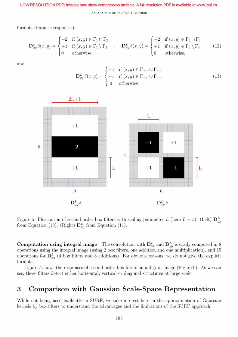
Figure 5: Illustration of second order box filters with scaling parameter L (here L = 5). (Left) DLyy
from Equation (10). (Right) DLxy from Equation (11).
Computation using integral image The convolution with DLxx and DL
yy is easily computed in 8operations using the integral image (using 2 box filters, one addition and one multiplication), and 15operations for DL
xy (4 box filters and 3 additions). For obvious reasons, we do not give the explicitformulas.
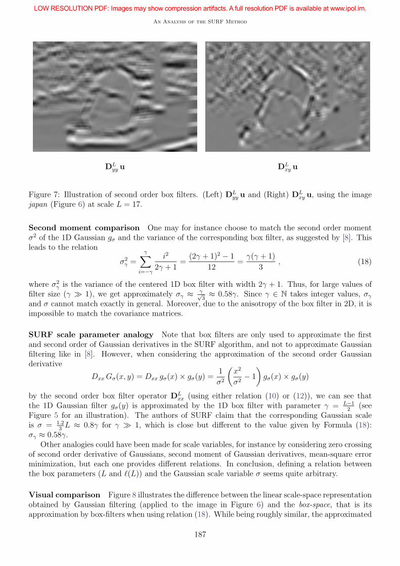
Figure 7 shows the responses of second order box filters on a digital image (Figure 6). As we cansee, these filters detect either horizontal, vertical or diagonal structures at large scale.
3 Comparison with Gaussian Scale-Space Representation
While not being used explicitly in SURF, we take interest here in the approximation of Gaussiankernels by box filters to understand the advantages and the limitations of the SURF approach.
185

Edouard Oyallon, Julien Rabin
Figure 6: Picture japan (image u), at resolution 481× 321 pixels.
3.1 Scale-Space Representation
Linear scale space The linear (Gaussian) scale-space representation of a real valued image u :R
2 7→ R defined on a continuous domain is obtained by a convolution with the Gaussian kernel
uσ := Gσ ∗ u, (14)
where Gσ is the centered, isotropic and separable 2-D Gaussian kernel with variance σ2
∀(x, y) ∈ R2, Gσ(x, y) :=
1
2πσ2e−
x2+y2
2σ2 = gσ(x) gσ(y) and gσ(x) =1√
2π · σe−
x2
2σ2 . (15)
The variable σ is usually referred to as the scale parameter.
Discrete scale space In practice, for the processing of a numerical image u, this continuous filteris approximated using regular sampling, truncation and normalization:
∀i, j ∈ J−K,KK Gσ(i, j) =1
CK
Gσ(i, j) , where CK =K∑
i,j=−K
Gσ(i, j). (16)
The scale variable σ is also sampled, generally using a power law, as discussed later in Section 3.2.
Discrete box space Making use of the aforementioned box filter technique, such a multi-scalerepresentation can be (very roughly) approximated using a box filter with square domain Γ =J−γ, γK× J−γ, γK
uγ :=1
(2γ + 1)2BΓ ∗ u. (17)
The question now is how to set the parameter γ ∈ N to get the best approximation of Gaussianzoom-out.
186
An Analysis of the SURF Method
DLyy u DL
xy u
Figure 7: Illustration of second order box filters. (Left) DLyy u and (Right) DL
xy u, using the imagejapan (Figure 6) at scale L = 17.
Second moment comparison One may for instance choose to match the second order momentσ2 of the 1D Gaussian gσ and the variance of the corresponding box filter, as suggested by [8]. Thisleads to the relation
σ2γ =
γ∑
i=−γ
i2
2γ + 1=
(2γ + 1)2 − 1
12=
γ(γ + 1)
3, (18)
where σ2γ is the variance of the centered 1D box filter with width 2γ + 1. Thus, for large values of
filter size (γ ≫ 1), we get approximately σγ ≈ γ√3≈ 0.58γ. Since γ ∈ N takes integer values, σγ
and σ cannot match exactly in general. Moreover, due to the anisotropy of the box filter in 2D, it isimpossible to match the covariance matrices.
SURF scale parameter analogy Note that box filters are only used to approximate the firstand second order of Gaussian derivatives in the SURF algorithm, and not to approximate Gaussianfiltering like in [8]. However, when considering the approximation of the second order Gaussianderivative
Dxx Gσ(x, y) = Dxx gσ(x)× gσ(y) =1
σ2
(
x2
σ2− 1
)
gσ(x)× gσ(y)
by the second order box filter operator DLxx (using either relation (10) or (12)), we can see that
the 1D Gaussian filter gσ(y) is approximated by the 1D box filter with parameter γ = L−12
(seeFigure 5 for an illustration). The authors of SURF claim that the corresponding Gaussian scaleis σ = 1.2
3L ≈ 0.8γ for γ ≫ 1, which is close but different to the value given by Formula (18):
σγ ≈ 0.58γ.Other analogies could have been made for scale variables, for instance by considering zero crossing
of second order derivative of Gaussians, second moment of Gaussian derivatives, mean-square errorminimization, but each one provides different relations. In conclusion, defining a relation betweenthe box parameters (L and ℓ(L)) and the Gaussian scale variable σ seems quite arbitrary.
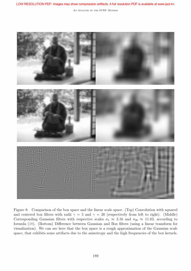
Visual comparison Figure 8 illustrates the difference between the linear scale-space representationobtained by Gaussian filtering (applied to the image in Figure 6) and the box-space, that is itsapproximation by box-filters when using relation (18). While being roughly similar, the approximated
187

Edouard Oyallon, Julien Rabin
scale-space exhibits some strong vertical and horizontal artifacts due to the anisotropy and the highfrequencies of the box kernels.
Again, whilst not being used explicitly in SURF, theses artifacts may explain some of the spuriousdetections of the SURF approach that will be exhibited later on.
3.2 Box-Space Sampling
Because of the definition of first and second order box filters, the size parameter L cannot be chosenarbitrarily. Table 2 shows the sampling values and the corresponding variables used to mimic thelinear scale space analysis. The following paragraphs give more detailed explanations.
o i σ(L) L 3L l(L) w(L)
1 1 1.2 3 9 2 0.9129
2 2.0 5 15 4 0.9487
3 2.8 7 21 6 0.9636
4 3.6 9 27 7 0.9718
2 1 2.0 5 15 4 0.9487
2 3.6 9 27 7 0.9718
3 5.2 13 39 10 0.9806
4 6.8 17 51 14 0.9852
3 1 3.6 9 27 7 0.9718
2 6.8 17 51 14 0.9852
3 10 25 75 20 0.9900
4 13.2 33 99 26 0.9924
4 1 6.8 17 51 14 0.9852
2 13.2 33 99 26 0.9924
3 19.6 49 147 39 0.9949
4 26.0 65 195 52 0.9962
Table 2: Box-space sampling values. The first two columns give the octave and level indexes. Thescale σ(L) defined in SURF by analogy to the linear scale space is given in the third column, usingEquation (20). The size parameter L = 2oi + 1 controls the width 2ℓ(L) + 1 of first order boxoperators DL
x and DLy through the relation ℓ(L) = ⌈0.8L⌋, and also the width 3L of second order
box filters DLxx, D
Lyy and DL
xy. The last column w(L) (Formula (26)) is required later to computethe determinant of Hessian (Section 4.1). The rows highlighted in bold font correspond to the scalesvalues that are finally used to describe the image. Other rows are only required for computationpurpose.
188
An Analysis of the SURF Method
Figure 8: Comparison of the box space and the linear scale space. (Top) Convolution with squaredand centered box filters with radii γ = 5 and γ = 20 (respectively from left to right). (Middle)Corresponding Gaussian filters with respective scales σ5 ≈ 3.16 and σ20 ≈ 11.83, according toformula (18). (Bottom) Difference between Gaussian and Box filters (using a linear transform forvisualization). We can see here that the box space is a rough approximation of the Gaussian scalespace, that exhibits some artifacts due to the anisotropy and the high frequencies of the box kernels.
189
Edouard Oyallon, Julien Rabin
Octave decomposition Alike most multi-scale decomposition approaches (see e.g. [14, 16]), thebox-space discretization in SURF relies on dyadic sampling of the scale parameter L. The box lengthrepresentation is therefore divided into octaves (similarly to SIFT [15, 14]), which are indexed byparameter o ∈ 1, 2, 3, 4, where a new octave is created for every doubling of the kernel size.
Note that, in order to save computation time, the filtered image is generally sub-sampled a factortwo at every octave, as done for instance by SIFT [15], so that the complexity remains the samethrough scales. As pointed out by the authors of SURF [2], the computation time complexity doesnot depend on scale when using box filters.
However, while not being explicitly stated in the original paper [2], but as done in most imple-mentations we have reviewed (for instance, this approximation is used in [3] but not in [5]), we stillchoose to use sub-sampling to speed-up the algorithm. More precisely, instead of evaluating themulti-scale operators at each pixel, we use a sampling “step” which depends on the octave level (thissampling is detailed in the next sections). Note that this strategy is consistent with the fact thatthe number of features is decreasing with respect to scale.
Scale sampling Each octave is also divided in several “levels” (indexed here by the parameteri ∈ 1, 2, 3, 4). In the usual discrete scale space analysis, these levels correspond directly to thedesired sampling of the scale variable σ, which parametrizes the discretized Gaussian kernels Gσ (seedefinition in Equation (16)). In SURF, the relation between scale L, octave o and level i variables is
L := 2o i+ 1 . (19)
These values are summarized in Table 2. Note that because of the non-maxima suppression involvedin the feature selection, only intermediate levels are actually used to define interest points and localdescriptors (i ∈ 2, 3). The corresponding scales are indicated by rows with bold font in Table 2.
Scale analogy with linear scale space As discussed before in Section 3.1, we can define a scaleanalysis variable by analogy with the linear scale space decomposition. In [2], the scale parameterσ(L) associated with octave o and level i is obtained by the following relation
σ(L) :=1.2
3(2o × i+ 1) = 0.4L. (20)
Since the relation between the scale σ(L) of an interest point is linear in the size parameter L of boxfilters operators, we shall speak indifferently of the former or the latter to indicate the scale.
Remark A finer scale-space representation could be obtained (i.e. with sub-pixel values of L)using a bilinear interpolation of the image, as suggested in [2]. This is not performed in the proposedimplementation.
3.3 Comparison with Gaussian Derivative Operators
3.3.1 First Order Operators
The first order box filters DLx and DL
y defined at scale L are approximations of the first deriva-tives of the Gaussian kernel Gσ at the corresponding scale σ(L) (see Equation (20)), respectivelycorresponding to
Dx Gσ(x, y) = −x
σ2(L)Gσ(x, y) and Dy Gσ(x, y).
These operators are used for local feature description, detailed in Section 5. Figure 9 compares thefirst order box filter impulse response with the discretized Gaussian derivative kernel.
190

An Analysis of the SURF Method
DLx δ (Equation (6)) Dx Gσ(L)
Figure 9: Comparison of Gaussian derivative with first order box filter. Illustration of the discretederivative operator DL
x (defined in Section 2.3.1) and discretization of the Gaussian derivative kernelDx Gσ(L) when using scale relation σ(L) from Equation (20).
Figure 10: Comparison of second order box filters and second order derivative of Gaussian kernels.(a) operator DL
yy; (b) discretized second order Gaussian derivative D2y Gσ; (c) operator DL
xy; (d)discretized second order Gaussian derivative Dxy Gσ; For comparison purpose, we used again thescale relation σ(L) from Equation (20).
3.3.2 The Second Order Operators
Second order differential operators are computed in the scale-space for the detection of interestpoints [12, 10]. In the linear scale-space representation, this boils down to the convolution withsecond derivatives of Gaussian kernels
Dxx Gσ(x, y) =1
σ2
(
x2
σ2− 1
)
Gσ(x, y), Dyy Gσ, and Dxy Gσ(x, y) =xy
σ4Gσ(x, y). (21)
In the SURF approach, the convolution with these kernels are approximated by second order boxfilters, previously introduced respectively as DL
xx, DLyy (Equation 10), and DL
xy (Equation 11). Avisual comparison between second order derivatives and their analogous with box filters is shown inFigure 10. These operators are required for the local feature selection step in Section 4.
3.3.3 Scale Normalization
According to [13], differential operators have to be normalized when applied in linear scale space inorder to achieve scale invariance detection of local features. More precisely, as it can be seen fromEquation (21), the amplitude of the continuous second order Gaussian derivative filters decreaseswith the scale variable σ by a factor 1
σ2 .
191
Edouard Oyallon, Julien Rabin
To balance this effect, second order operators are usually normalized by σ2, so that we get forinstance
• the scale-normalized determinant of Hessian operator:
DoHσ (u) :=
∣
∣
∣
∣
∣
∣
∣
σ2
Dxx Dxy
Dyx Dyy
uσ
∣
∣
∣
∣
∣
∣
∣
= σ4[
Dxx uσ ·Dyy uσ − (Dxy uσ)2] ; (22)
• the scale-normalized Laplacian operator:
∆σ u := σ2∆ uσ = σ2∆ Gσ ∗ u = σ2(Dxx +Dyy)Gσ ∗ u = σ2(Dxx uσ +Dyy uσ) , (23)
where ∆σ Gσ(x, y) = σ2(Dxx+Dyy) Gσ(x, y) =(
x2+y2
σ2 − 1)
Gσ(x, y) is the multi-scale Lapla-
cian of Gaussian. Observe that this operator can be obtained from the trace of the scale-normalized Hessian matrix.
These two operators are widely used in computer vision for feature detection. They are alsoapproximated in SURF, as detailed in the next sections. As a consequence, such a scale-normalizationis also required with box filters to achieve similar invariance in SURF. To do so, the authors ofSURF proposed that the amplitude of operators DL
xx (Equation 10), DLyy (Equation 10), and DL
xy
(Equation 11) should be reweighted so that the l2 norms of normalized operators become constantover scales.
The quadratic l2 norm of operators are estimated from the squared Frobenius norm of impulseresponses
‖DLxx‖
2
2 := ‖DLxx δ‖
2
F = ‖DLyy δ‖
2
F=
(
1 + 1 + (−1)2)
L(2L− 1) = 6L(2L− 1),
so that ‖DLxx‖
2
2 ≈ 12L2 when L≫ 1, and
‖DLxy‖
2
2:= ‖DL
xy δ‖2
F=
(
1 + 1 + (−1)2 + (−1)2)
L× L = 4L2.
This means that box filters responses should be simply divided by the scale parameter L to achievescale invariance detection.
4 Interest Point Detection
In the previous sections, second order operators based on box filters have been introduced. Theseoperators are multi-scale and may be normalized to yield scale invariant response. We will nowtake interest in their use for multi-scale local feature detection. Once the integral image has beencomputed, three consecutive steps are performed:
1. Feature filtering (Section 4.1) based on a combination of second order box filters;
2. Feature selection (Section 4.2) combining non-maxima suppression and thresholding;
3. Scale-space location refinement (Section 4.3) using second order interpolation.
This interest point detection task is summarized in Algorithm 1.
192

An Analysis of the SURF Method
Algorithm 1 Detection of interest points
input: image u
output: listKeyPoints(Initialization)U← IntegralImage(u) (Equation (1))(Step 1: filtering of features)for L ∈ 3, 5, 7, 9, 13, 17, 25, 33, 49, 65 do (scale sampling, according to Table 2)
DoHL(u)←Determinant of Hessian (U, L) (See Equation (24) and Algorithm 2)end for
(Step 2: selection and refinement of keypoints)for o := 1 to 4 do (octave sampling)
for i := 2 to 3 do (levels sampling for maxima location)L← 2oi+ 1 (Equation (19))listKeyPoints← listKeyPoints + KeyPoints(o, i,DoHL(u)) (See Section 4.2 and Algo-
rithm 3)end for
end for
return listKeyPoints
4.1 Feature Filtering
The objective is to detect interesting features in the box-space which are highly discriminant, suchas corners, junctions (intersection of edges), blobs, etc. Taking inspiration from the previous worksof Lindeberg [12, 10, 11, 13] about scale-invariant detection, SURF [1, 2] uses scale-normalizeddeterminant of Hessian to detect saddle points in images. Note that other popular methods are thenormalized Laplacian detector (Equation (23)), scale invariant Harris corner detector [18], or affineinvariant blob detector [17].
Determinant of Hessian using box filters The scale-normalized determinant of Hessian matrixoperator proposed in SURF is defined as follows
DoHL(u) :=1
L4
(
DLxx u ·DL
yy u−(
w DLxy u
)2)
, (24)
using the scaling relation L = 2oi + 1, and a constant weighting factor w = 0.912. As mentionedearlier, the normalization factor 1
L4 is required to ensure scale invariance. The weighting factor w isused to compensate the numerical approximation of the Hessian determinant by box filters. We willdiscuss later on these two aspects. An illustration of this multi-scale structure detector is given inFigure 11.
Computation using integral image At each point of the box-space, the computation of thisoperator requires 36 operations: (8 × 2 + 15) to evaluate box filters, plus 4 multiplications and 1addition. The method to compute the DoHL(u) at a given scale is described in Algorithm 2.
Sampling As mentioned before, it is not necessary to evaluate the Hessian determinant for everypixel at large scale. To reduce computation time, the operator response is sampled according to theoctave level o, such that the number of points tested per octave is ⌈ M
2o−1 ⌉ × ⌈ N2o−1 ⌉. In Algorithm 2,
this sub-sampling strategy corresponds to a sampling step p = 2o−1.
193

Edouard Oyallon, Julien Rabin
DoHL u (Equation (22)) DoHσ u (Equation (23))
Figure 11: Determinant of Hessian Operators applied to the images japan (top row) and lena (bot-tom), either using box filters operator DoHL at scale L = 9 (left column) or Gaussian derivativefilter DoHσ at scale σ(L) = 0.4L = 3.6 (right column).
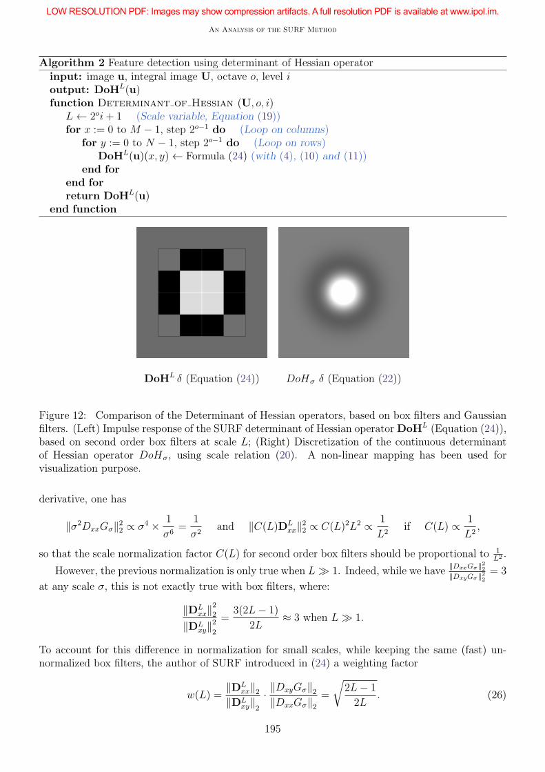
Normalization and analogy with continuous determinant of Hessian Recall that the Hes-sian determinant based on box filters aims at approximating the DoHσ operator defined in For-mula (22). The comparison of their impulse responses is shown in Figure 12. As previously stated,the box filters are not isotropic, which may be source of strong horizontal and vertical artifacts: thiscan be observed in Figure 11.
Moreover, recall that to achieve scale invariance, the multi-scale operator response has to benormalized so that the l2 norm remains constant over scales. This is the role of the denominator L4
in (24). Indeed, from Section 3.3.3 we know that ‖Dxx
L‖22 = ‖Dyy
L‖22 ≈ 12L2 and ‖Dxy
L‖22 = 4L2
(see Section 3.3.3). On the other hand, we can show that
‖DxxGσ‖22 =3
16πσ6= 3‖DxyGσ‖22 . (25)
By simple analogy between the two approaches, for instance considering the normalized Gaussian
194
An Analysis of the SURF Method
Algorithm 2 Feature detection using determinant of Hessian operator
input: image u, integral image U, octave o, level ioutput: DoHL(u)function Determinant of Hessian (U, o, i)
L← 2oi+ 1 (Scale variable, Equation (19))for x := 0 to M − 1, step 2o−1 do (Loop on columns)
for y := 0 to N − 1, step 2o−1 do (Loop on rows)DoHL(u)(x, y)← Formula (24) (with (4), (10) and (11))
end for
end for
return DoHL(u)end function
DoHL δ (Equation (24)) DoHσ δ (Equation (22))
Figure 12: Comparison of the Determinant of Hessian operators, based on box filters and Gaussianfilters. (Left) Impulse response of the SURF determinant of Hessian operatorDoHL (Equation (24)),based on second order box filters at scale L; (Right) Discretization of the continuous determinantof Hessian operator DoHσ, using scale relation (20). A non-linear mapping has been used forvisualization purpose.
derivative, one has
‖σ2DxxGσ‖22 ∝ σ4 × 1
σ6=
1
σ2and ‖C(L)DL
xx‖22 ∝ C(L)2L2 ∝ 1
L2if C(L) ∝ 1
L2,
so that the scale normalization factor C(L) for second order box filters should be proportional to 1L2 .
However, the previous normalization is only true when L≫ 1. Indeed, while we have‖DxxGσ‖22‖DxyGσ‖22
= 3
at any scale σ, this is not exactly true with box filters, where:
‖DLxx‖
2
2
‖DLxy‖22
=3(2L− 1)
2L≈ 3 when L≫ 1.
To account for this difference in normalization for small scales, while keeping the same (fast) un-normalized box filters, the author of SURF introduced in (24) a weighting factor
w(L) =‖DL
xx‖2‖DL
xy‖2· ‖DxyGσ‖2‖DxxGσ‖2
=
√
2L− 1
2L. (26)
195

Edouard Oyallon, Julien Rabin
The numerical values of this parameter are listed in the last column of Table 2. As noticed by theauthors of SURF, the variable w(L) does not vary so much across scales. This is the reason why theweighting parameter w in Equation (24) is fixed to w(3) = 0.9129.
4.2 Feature Selection
A point of interest is a point of the box-space that is approximately covariant to any similarity ofthe initial image u. The term covariant implies here that the surrounding region covariantly changeswith the considered class of transformation. To design a descriptor invariant to similarities, theselection of the interest point is jointly performed with the estimation of the similarity transformparameters (location, scale and orientation).
In the SURF methodology, interest points are defined as local maxima of the aforementionedDoHL operator applied to the image u. These maxima are detected by considering a 3 × 3 × 3neighborhood, and performing an exhaustive comparison of every voxel of the discrete box-space withits 26 nearest-neighbors. The corresponding feature selection procedure is described in Algorithm 3.
Algorithm 3 Selection of features
input: o, i,DoHL(u), tH (Determinant of Hessian response at octave o and level i)output: listKeyPoints (List of keypoints in box space with sub-pixel coordinates (x,y,L))function KeyPoints (o, i,DoHL(u))
L← 2oi+ 1for x := 0 to M − 1, step 2o−1 do (Loop on columns)
for y = 0 to N − 1, step 2o−1 do (Loop on rows)if DoHL(u)(x, y) > tH then (Thresholding, Equation (27))
if isMaximum (DoHL(u), x, y) then (Non-maximum suppression)if isRefined (DoHL(u), x, y, L) then (Refinement by interpolation, Sec-
tion 4.3)addListKeyPoints (x, y, L)
end if
end if
end if
end for
end for
return listKeyPointsend function
Remark A faster method has been proposed in [22] to find the local maxima without exhaustivesearch, which has been not implemented for the demo.
Thresholding Using four octaves and two levels for analysis, eight different scales are thereforeanalyzed (see Table 2 in Section 3.2). In order to obtain a compact representation of the image -andalso to cope with noise perturbation- the algorithm selects the most salient features from this set oflocal maxima. This is achieved by using a threshold tH on the response of the DoHL operator
DoHL(u)(x, y) > tH . (27)
Note that, since the operator is scale-normalized, the threshold is constant. In the demo, we settH = 103 assuming that the input image u takes values in the interval J0, 255K. This setting enablesus to have a performance similar to the original SURF algorithm [2, 1] (see Section 6 for more details).
196
An Analysis of the SURF Method
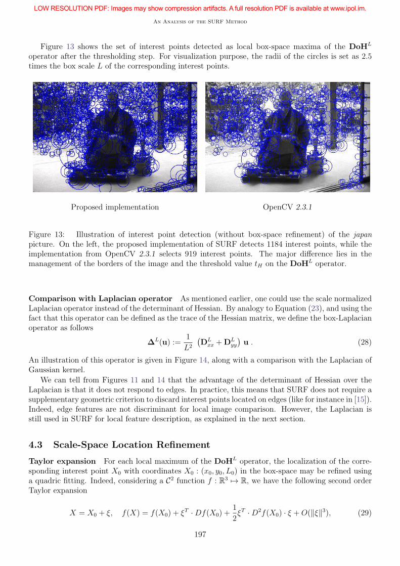
Figure 13 shows the set of interest points detected as local box-space maxima of the DoHL
operator after the thresholding step. For visualization purpose, the radii of the circles is set as 2.5times the box scale L of the corresponding interest points.
Proposed implementation OpenCV 2.3.1
Figure 13: Illustration of interest point detection (without box-space refinement) of the japanpicture. On the left, the proposed implementation of SURF detects 1184 interest points, while theimplementation from OpenCV 2.3.1 selects 919 interest points. The major difference lies in themanagement of the borders of the image and the threshold value tH on the DoHL operator.
Comparison with Laplacian operator As mentioned earlier, one could use the scale normalizedLaplacian operator instead of the determinant of Hessian. By analogy to Equation (23), and using thefact that this operator can be defined as the trace of the Hessian matrix, we define the box-Laplacianoperator as follows
∆L(u) :=1
L2
(
DLxx +DL
yy
)
u . (28)
An illustration of this operator is given in Figure 14, along with a comparison with the Laplacian ofGaussian kernel.
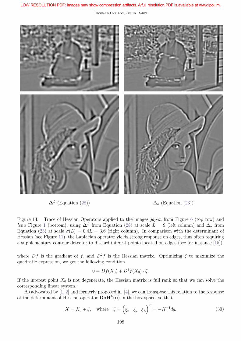
We can tell from Figures 11 and 14 that the advantage of the determinant of Hessian over theLaplacian is that it does not respond to edges. In practice, this means that SURF does not require asupplementary geometric criterion to discard interest points located on edges (like for instance in [15]).Indeed, edge features are not discriminant for local image comparison. However, the Laplacian isstill used in SURF for local feature description, as explained in the next section.
4.3 Scale-Space Location Refinement
Taylor expansion For each local maximum of the DoHL operator, the localization of the corre-sponding interest point X0 with coordinates X0 : (x0, y0, L0) in the box-space may be refined usinga quadric fitting. Indeed, considering a C2 function f : R3 7→ R, we have the following second orderTaylor expansion
X = X0 + ξ, f(X) = f(X0) + ξT ·Df(X0) +1
2ξT ·D2f(X0) · ξ +O(‖ξ‖3), (29)
197
Edouard Oyallon, Julien Rabin
∆L (Equation (28)) ∆σ (Equation (23))
Figure 14: Trace of Hessian Operators applied to the images japan from Figure 6 (top row) andlena Figure 1 (bottom), using ∆L from Equation (28) at scale L = 9 (left column) and ∆σ fromEquation (23) at scale σ(L) = 0.4L = 3.6 (right column). In comparison with the determinant ofHessian (see Figure 11), the Laplacian operator yields strong response on edges, thus often requiringa supplementary contour detector to discard interest points located on edges (see for instance [15]).
where Df is the gradient of f , and D2f is the Hessian matrix. Optimizing ξ to maximize thequadratic expression, we get the following condition
0 = Df(X0) +D2f(X0) · ξ.
If the interest point X0 is not degenerate, the Hessian matrix is full rank so that we can solve thecorresponding linear system.
As advocated by [1, 2] and formerly proposed in [4], we can transpose this relation to the responseof the determinant of Hessian operator DoHL(u) in the box space, so that
X = X0 + ξ, where ξ =(
ξx ξy ξL
)T
= −H−10 d0. (30)
198

An Analysis of the SURF Method
In the previous expression, L is the scale variable, and d0 and H0 are the discrete gradient and thediscrete Hessian of DoHL(u) at point X0 = (x0, y0, L0), respectively denoted as follows
d0 =
dx
dy
dL
H0 =
Hxx Hxy HxL
Hxy Hyy HyL
HxL HyL HLL
.
The numerical evaluation of the components of the gradient vector d0 and the symmetric Hessianmatrix H0 of DoHL0(u) at scale L0 and location (x0, y0) is obtained from finite difference schemesin the box space, with a 3× 3× 3 centered neighborhood.
Finite difference scheme for gradient and Hessian matrix estimation Taking into accountthat a sub-sampling is performed with a step parameter p = 2o−1 which is scale dependent, expressionsare quite straightforward for the derivative according to spatial coordinates, with ∀X0 ∈ Ω× L
dx(X0) =1
2p
(
DoHL0(u)(x0 + p, y0)−DoHL0(u))(x0 − p, y0))
, (31)
Hxx(X0) =1
p2
(
DoHL0(u)(x0 + p, y0) +DoHL0(u)(x0 − p, y0)− 2DoHL0(u)(x0, y0))
, (32)
Hxy(X0) =1
4p2[
+DoHL0(u)(x0 + p, y0 + p) +DoHL0(u)(x0 − p, y0 − p)
− DoHL0(u)(x0 − p, y0 + p)−DoHL0(u)(x0 + p, y0 − p)]
. (33)
Special care has to be given for the processing of the scale coordinate, since this time the samplingis done (see Equation 19). Using the chain rule, and ∂L
∂i= 2o = 2p, one thus has
dL(X0) =∂i
∂Ldi(X0) =
1
4p
(
DoHL0+2p(u)(x0, y0)−DoHL0−2p(u))(x0, y0))
, (34)
HxL(X0) =1
8p2[
+DoHL0+2p(u)(x0 + p, y0) +DoHL0−2p(u)(x0 − p, y0)
− DoHL0+2p(u)(x0 − p, y0)−DoHL0−2p(u)(x0 + p, y0)]
, (35)
HLL(X0) =1
4p2(
DoHL0+2p(u)(x0, y0) +DoHL0−2p(u))(x0, y0)− 2DoHL0(u)(x0, y0))
. (36)
Refinement rejection It is possible that the refined point X = X0 + ξ does not belong to theneighborhood of X, i.e. max(|ξx|, |ξy|, 12 |ξL|) > p. This happens if the Hessian matrix is ill condi-tioned. In practice, those interest points are not reliable for matching and are thus discarded, asproposed in [4]. The location refinement procedure is described in Algorithm 4 and is illustrated inFigure 15.
199
Edouard Oyallon, Julien Rabin
Algorithm 4 Box-space location refinement
input: X0 : (x0, y0, L0) and DoHL(u) (Refinement in box-space of detected point X0 at scaleL0 = 2oi+ 1)output: True/False & X : (x, y, L) (Is the interest point kept ? If so, return the position ofthe refined detected point.)function isRefined (DoHL(u), X0)
p← 2o−1 (Step parameter for finite different scheme)H0 ← Formulas (32), (33), (35) and (36). (Hessian matrix)d0 ← Formulas (31) and (34). (Gradient vector)ξ ← −H0
−1 · d0 (Maximum refinement, see Equation (30))if max(|ξx|, |ξy|, 12 |ξL|) < p then (Check precision improvement)
(x, y, L) ← (x0, y0, L0) + ξ (Refinement using 2nd order Taylor expansion, see Equa-tion (29))
return True, X : (x, y, L)else
return False
end if
end function
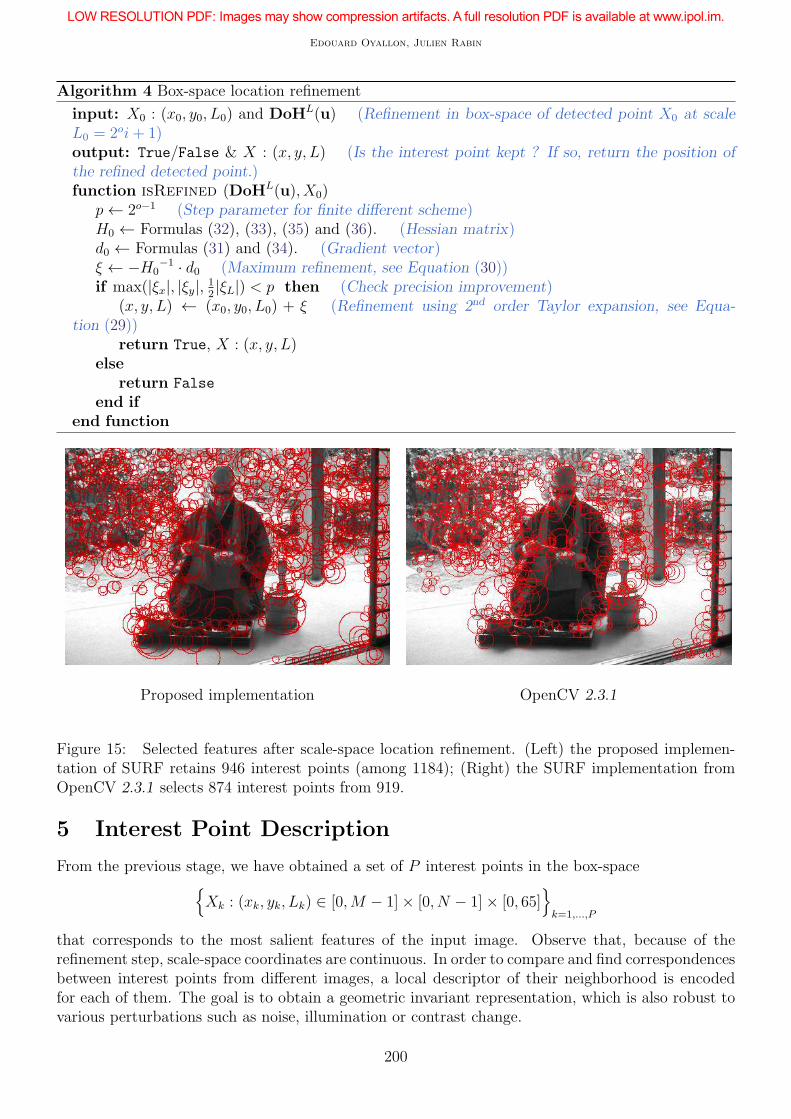
Proposed implementation OpenCV 2.3.1
Figure 15: Selected features after scale-space location refinement. (Left) the proposed implemen-tation of SURF retains 946 interest points (among 1184); (Right) the SURF implementation fromOpenCV 2.3.1 selects 874 interest points from 919.
5 Interest Point Description
From the previous stage, we have obtained a set of P interest points in the box-space
Xk : (xk, yk, Lk) ∈ [0,M − 1]× [0, N − 1]× [0, 65]
k=1,...,P
that corresponds to the most salient features of the input image. Observe that, because of therefinement step, scale-space coordinates are continuous. In order to compare and find correspondencesbetween interest points from different images, a local descriptor of their neighborhood is encodedfor each of them. The goal is to obtain a geometric invariant representation, which is also robust tovarious perturbations such as noise, illumination or contrast change.
200
An Analysis of the SURF Method
The scale space analysis already offers scale and translation invariance. To achieve similarityinvariance, one also needs rotational invariance. One way to achieve this consists in extracting foreach interest point a dominant orientation following the procedure detailed in Section 5.2. Then,SURF features are built from the normalized gradient distribution in the vicinity of interest points(Section 5.3). Finally, a method to compare SURF descriptors and find local correspondences betweenimages is exposed in Section 5.4.
5.1 Scale of an Interest Point
In the previous section, for the sake of simplicity, we have referred to L as the scale parameter ofthe box-space. Let us now recall that the analogous relation between the box-filter size parameterL and the equivalent scale variable σ from linear scale space is given by Equation (20). Thus, for agiven detected feature point Xk, one has the corresponding scale variable
σk = ⌊0.4Lk⌉. (37)
This scale variable is used thoroughly in the following sections to define various scale normalizationsinvolved in SURF descriptors. Note that the rounding operator ⌊·⌉ is only required for numericalconvenience.
5.2 Dominant Orientation of an Interest Point
Alike the SIFT method, the main orientations of SURF keypoints are computed from the localdistribution of the gradient orientation.
Weighted gradient computation For each interest point Xk, we first consider the neighborhoodB6σk
(xk, yk) defined as the disk of radius 6σk with center (xk, yk). The computation of the gradientat this scale σk, and in this neighborhood B6σk
(xk, yk) is obtained by convolution with first order boxfilters (see the corresponding definition of DLk
x (Equation (6)) and DLky (Equation (7))). To reduce
the impact of remote pixels, the gradient samples are weighted according to their distance from theinterest point, using a discrete Gaussian kernel (Equation (16)), with a standard deviation equal to2σk. The weighted gradient at point (x, y) then writes (x and y being integer coordinates of the pixelgrid Ω)
∀(x, y) ∈ Ω ∩ B6σk(xk, yk), φk(x, y) :=
DLkx
DLky
u(x, y) ·G1
(
x− xk
2σk
,y − yk
2σk
)
. (38)
Orientation score function Unlike the SIFT approach in which a histogram is built from gradientsamples to estimate the dominant orientation [15], SURF computes the following score vector Φaccording to the orientation θ
Φk(θ) =∑
(x,y)∈B6σk(x
k,y
k)
φk(x, y)× 1[θ−π6,θ+π
6] (∠φk(x, y)). (39)
This vector sums all the weighted gradients in the considered neighborhood which have approximatelythe same orientation θ (with a fixed tolerance of ±π
6). Here, ∠φ ∈ [−π, π) denotes the angle between
vector φ ∈ R2 and canonical vector (1, 0)T 2. The orientation score function is defined as the l2
norm of this aggregated vector ‖Φk(θ)‖.2 This corresponds to the C++ standard math library function atan2.
201
Edouard Oyallon, Julien Rabin
Dominant orientation Finally, the orientation of the interest point Xk is defined as the globalmaximum of the orientation score function
θk = ∠Φk(θ⋆) where θ⋆ ∈ argmax
θ∈Θ‖Φk(θ)‖. (40)
In the proposed demo, we evaluate the orientation score function for 40 different angles, uniformlysampled over the unit circle: Θ =
kπ20, k = 0, 1, . . . , 39
.An example of dominant orientation estimation is given in Figure 16, in which the estimated
orientations are represented by segments. Algorithm 5 summarizes the computation of the mainorientation of an interest point.
Algorithm 5 Computation of the orientation
input: u, X : (x, y, L)output: θ (Main orientation of the interest point neighborhood)function Orientation (u, x, y, L)
σ ← ⌈0.4L⌋ (Scale variable definition from Equation (37))for i := −6 to 6 do (Span the keypoint neighborhood)
for j := −6 to 6 do
if i2 + j2 ≤ 36 then (Check that (x+ iσ, y + jσ) ∈ B6σ(x, y))φ(i,j) =
(
DLx ,D
Ly
)T u(x+iσ, y+jσ)×G1
(
i2, j
2
)
(Using Equation (43), Equation (6)and (7))
end if
end for
end for
for k := 0 to 39 do (Span the discrete set of tested angular sector Θ)θk ← kπ
20(Θ = θkk)
Φ(θk)← Formula (39) (Compute orientation score function for angular sector θk)end for
θ⋆ = argmaxθ∈Θ
‖Ψ(θ)‖ according to Formula (40)
return θ = ∠Φ(θ⋆)end function
Sampling strategies Once again, as previously done for interest point detection, a sub-samplingstrategy is used to speed up the SURF descriptor construction. Indeed, the weighted gradientoperator is not computed in practice for all the pixels from the neighborhood, which would be com-putationally prohibitive for large scales. Instead, pixel locations are sampled with a step parameterequal to the scale of the interest point σk, as explicitly detailed in Algorithm 5. Another advantageof this strategy is that the number of gradient samples used to estimate the main orientation isconsistent throughout the scales (approximately 100 samples in our implementation).
5.3 SURF Descriptors
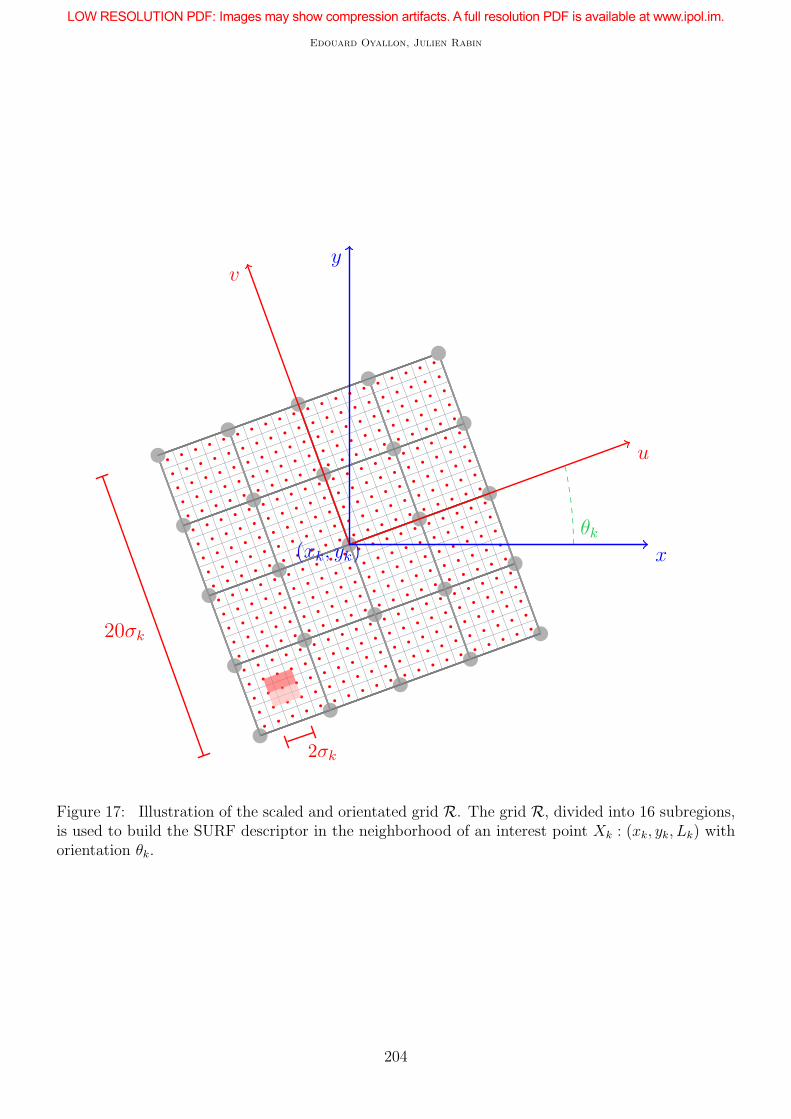
A SURF descriptor is a 16×4 vector, representing normalized gradient statistics (mean and absolutemean values) extracted from a spatial grid R divided into 4-by-4 regions. These subregions arereferred to as R = Ri,j1≤i,j≤4. For a given oriented interest point Xk : (xk, yk, Lk, θk), as illustratedin Figure 17, the corresponding square grid is centered at (xk, yk), aligned according to θk and scaledto have a normalized width of 20σk, using relation (37).
202

An Analysis of the SURF Method
Ipol logo (705× 323 pixels)
Proposed implementation of SURF
SURF algorithm from OpenCV 2.3.1
Figure 16: Illustration of interest points detection with dominant orientation. The radius of thecircle indicates the scale of the interest point and the segment shows the selected orientation basedon Algorithm 5. (Middle) 456 points are detected with the proposed implementation of SURF.(Bottom) 478 interest point are selected with the SURF implementation of OpenCV 2.3.1.
203
Edouard Oyallon, Julien Rabin
2σk
(xk, yk)
20σk
v
u
θk
y
x
Figure 17: Illustration of the scaled and orientated grid R. The grid R, divided into 16 subregions,is used to build the SURF descriptor in the neighborhood of an interest point Xk : (xk, yk, Lk) withorientation θk.
204

An Analysis of the SURF Method
Scale normalized sampling A subregion Ri,j is a square with side length equal to 5σk. Gradientresponses are regularly sampled, using a step equal to σk. Hence, 25 gradients are consistently usedin each subregion to build the SURF descriptor for any interest point.
Change of coordinates The coordinates of gradient samples according to the descriptor grid aredenoted by (u, v) whereas the coordinates on the pixel grid Ω are denoted (x, y). The similaritytransform between the two coordinate systems is then
Sk :
(
u
v
)
7→(
x
y
)
= σk ·Rθk
(
u
v
)
+
(
xk
yk
)
, where Rα =
(
cosα − sinα
sinα cosα
)
. (41)
To span the grid R, one must take u, v ∈ J−10, 9K+ 12(where the term 1
2is used to ensure symmetry).
Since the coordinates (x, y) do not correspond exactly to pixel values, rounding is required (nearestneighbor interpolation)
(x,y) = ⌊Sk(u, v)⌉ = (⌊x⌉, ⌊y⌉) ∈ Ω. (42)
Note also that the coordinates of (u, v) implicitly depend on the subregion coordinates Ri,j (seeAlgorithm 6 for more details).
Gradient normalization The gradient components are computed by convolution with first orderbox filters DLk
x and DLky (see Formulas (6) and (7)). To avoid the use of interpolation due to the
orientation of the descriptor grid R, the gradients responses are first computed on the regular gridΩ, and then rotated using rotation matrix R−θk to cancel the descriptor orientation.
In addition, as previously done for the dominant orientation selection, the gradient responsesare weighted according to the distance of the pixel from the interest point. This processing aims atreducing the importance of distant pixels which are more sensitive to orientation or scale perturbation.In SURF [2], the weights are defined by a discrete Gaussian kernel (Equation (16)), with a standarddeviation equal to 3.3 σk.
Eventually, the weighted gradient at point (u, v) reads
∀ (u, v) ∈ R,
dx(u, v)
dy(u, v)
:= R−θk
DLkx
DLky
u (x,y)×G1
( u
3.3,v
3.3
)
. (43)
Gradient statistics Similarly to SIFT, the SURF descriptor aggregates local gradient informationfrom subregions. However, whereas SIFT builds small histograms of gradient orientations (weightedby gradient magnitude), SURF computes first order statistics on vertical and horizontal gradientresponses. The authors of SURF [2] claim that using the sum and the sum of absolute values yieldsthe best compromise between compactness and efficiency. The resulting statistical vector describingsubregion Ri,j corresponds to
∀ (i, j) ∈ J1, 4K2 , µk(i, j) =
∑
(u,v)∈Ri,jdx(u, v)
∑
(u,v)∈Ri,jdy(u, v)
∑
(u,v)∈Ri,j| dx(u, v) |
∑
(u,v)∈Ri,j| dy(u, v) |
. (44)
205

Edouard Oyallon, Julien Rabin
The SURF descriptor associated to the interest point Xk : (xk, yk, Lk, θk) is then simply obtainedby concatenating the 16 vectors µk(i, j) computed for every subregion
µk =(
µk(i, j))
1≤i,j≤4. (45)
Descriptor normalization The previous geometric normalization guaranties invariance to simi-larity transforms. In practice, the use of local gradient information combined with a localization gridR yields also robustness to small changes of viewpoint. In order to gain invariance to linear contrastchanges, the SURF descriptor is normalized to a unit vector, using Euclidean norm
surf(Xk) =µk
‖µk‖2. (46)
Besides, because of this l2 normalization, it is unnecessary to use scale-normalized first order boxfilters.
The construction of such descriptor is summarized in Algorithm 6.
Sign of the Laplacian Eventually, for each interest point Xk, in addition to scale-space coordi-nates (xk, yk, Lk) and orientation θk, the local sign of the Laplacian is also stored. The approximateLaplacian operator response is obtained from ∆Lk u(xk, yk), using Formula (28). The goal is to ac-celerate the comparison of of SURF interest points during the matching step (see Section (5.4) formore details). The sign of the Laplacian response provides some information about the local contrastof the interest point. Since this operator is the trace of the readily available Hessian matrix, thisoperator only requires one additional operation.
Algorithm 6 Construction of SURF descriptor
input: Input image u, keypoint X : (x, y, L)output: SURF Descriptor, orientation of keypoint and sign of Laplacianfunction buildDescriptor (u, x, y, L)
θ ← Orientation (u, x, y, L) (See Algorithm 5)for i := 1 to 4 do (Span the 4-by-4 subregions Ri,j of the oriented grid)
for j := 1 to 4 do
for u := −9.5 to 9.5 step 1 do (Span the subregions Ri,j coordinates (u, v))for v := −9.5 to 9.5 step 1 do
(x, y) = S(u, v) (Change of coordinates, see Formula (41))(x,y) = ⌊(x, y)⌉ (Nearest neighbor pixel, see Formula (42))DLk
x u(x,y), DLky u(x,y) (Gradient response)
(dx(u, v), dy(u, v))← Formula (43) (Gradient correction)end for
end for
µ(i, j)← Formula (44) (Compute subregion statistical descriptor ∈ R4)
end for
end for
µ← concatenate (µk(i, j)1≤i,j≤4) (16× 4 dimensional vector (Equation (45)))surf(X)← normalize (µ) (l2 normalization (Equation (46)))∆L(u)(x, y)← Formula (28) (Laplacian at scale L)return surf(X), θ, Sign(∆L(u)(x, y))
end function
206

An Analysis of the SURF Method
5.4 Feature Matching
From the previous steps, a pair of images (u,v) to be matched is represented by two sets of interestpoints (Xkk and Yll) with their corresponding SURF descriptors (surf(Xk)k and surf(Yl)l).Recall that a SURF descriptor X ∈ [−1, 1]64 is a 64-dimensional vector with unitary Euclidean norm:‖X‖ = 1. The matching step is simply performed here as an exhaustive comparison of these vectorsusing Euclidean distance, combined with a Nearest-Neighbor Distance Ratio (NN-DR) thresholdingtechnique.
Feature comparison For any query descriptor Xk from the first image u, we compute the Eu-clidean distance d2k,l = ‖Xk−Yl‖22 = 2(1−XT
k ·Yl) with all the candidate features Yl from the secondimage v. Since around a thousand of SURF features are approximately extracted from a 1 megapixelimage, millions of scalar products are therefore computed.
To speed up the matching procedure, we first compare the signs of the Laplacian of SURF featuresas advocated by the authors of SURF. If the signs of two descriptors are different, they are veryunlikely similar: the distance is therefore not computed and the potential match is discarded.
Besides, note that many other methods exist in the literature to accelerate the comparison ofvectors, either for exact or approximate Nearest-Neighbor search, based on data structure (such asKd-tree, Vector quantization, etc.). We did not use such techniques in the proposed source code.
Matching criterion Subsequently, one needs to extract the most significant correspondences fromwithin typically several millions of putative ones. In other words, taking only the similarity distancesdk,l into account, one has to separate the correct matches from the spurious ones. A classic paradigmis the nearest neighbor matching, which consists in testing only correspondences between each querydescriptor Xk with its most similar candidate, denoted by Yl1 where
l1 ∈ argminl
dk,l .
The Nearest Neighbor Distance Threshold (NN-DT) is a straightforward technique to validate sucha putative correspondence based on a fixed threshold on the similarity measure. Inescapably, such amatching criterion implies a compromise between the number of false positives and false negatives.
As done in SURF [2], we use instead the NN-DR matching criterion, a simple statistical methodproposed by Lowe [15] to discard mismatches, which has been shown (see e.g. [23]) to outperformNN-DT. This method considers the ratio between the first and second nearest neighbors to measurethe quality of a correspondence between the query and the most similar candidate. Thus, we firstcompute the closest Yl1 and second closest Yl2 candidates from the query feature Xk, such that
l2 ∈ argminl, s.t. dk,l≥dk,l1
dk,l.
and then compare the corresponding ratio of distances to a fixed threshold t, so that
ifdk,l1dk,l2
≤ t ⇔ correspondence (Xk, Yl1) is validated.
Following [15], in our experiments, the threshold was set to t = 0.8.
Geometric consistency Finding local correspondences between two images is rarely an end initself. In practice, one wants for instance to find the geometric deformation between the two images(image registration) or decide if they share a similar object (object detection and recognition). More-over, the previous matching criterion is generally not sufficient to discard most mismatches. Thus,
207

Edouard Oyallon, Julien Rabin
in the demonstration, we decided to incorporate an optional and additional matching criterion basedon the epipolar geometry consistency. To do so, we use the ORSA algorithm [21], which combinesthe RANSAC [6] algorithm with hypothesis testing.
Without going into details (see for instance [20]) this supplementary criterion consists in findingthe most significant geometric relation between the two images to remove correspondences that arenot consistent with it. More specifically, we consider the two images as two different views of thesame scene (stereo-vision). The epipolar geometry enables to account for the perspective deformationbetween the coordinates of corresponding interest points in the two images. Random subsets ofcorrespondences are iteratively drawn and used to estimate the related fundamental matrix. Givena tolerance error, the matches that are consistent with the geometry are counted to select the bestgeometric transformation between the two images.
This supplementary criterion is also given in the proposed source code and is used in the followingsection for visualization purpose
6 Experiments
In this section, we illustrate the performance of the SURF algorithm for image matching. We firstevaluate the validity of the proposed implementation by checking the SURF properties: invariance tosimilarity transform and robustness to small viewpoint changes. Secondly, some examples of imagepair matching are shown to illustrate the behavior (both success and failure) of the SURF method,along with a comparison with some other competitive methods.
6.1 Performance Evaluation
An executable program has been released by the authors of SURF 3. Unfortunately, we were only ableto use it partially. So, in order to evaluate and validate our implementation of the SURF algorithm,some of the benchmarks proposed in [2] have been reproduced.
In these benchmarks, performance curves are obtained from the experimental protocol from [19]which provides several image sequences with geometric distortion (along with the ground-truth) andthe MATLAB code to compute scores. Two different types of performance measures are evaluated toassess the quality of the feature detection and description: the repeatability score and the precision-recall rate.
Repeatability The repeatability score represents the proportion of nearly identical features de-tected in two different views of the same scene.
Let u be the image of interest, and u′ be the same reference scene from a different viewpoint,so that the transform T between the two view is known (in practice, a homography combined witha mask). For each point Xk selected in u, an ideal detector should find the same interest point X ′
k
in u′, such that Xk = T (X ′k). The repeatability test consists in measuring how often this relation
is verified. In practice, due to numerical approximations (blur, noise, quantization, errors, etc) thatresult in u ≈ T (u′), we have to test for each Xk if there is some detected point X ′
i in u′ which isclose enough. To this end, and following [19], we consider the support region Rk of each keypointXk, here defined as a disk Bs(xk, yk) centered on the point location and which radius s is fixed (30pixels in [19]). Two keypoints Xk and X ′
i are considered similar if the overlap error between thetwo registered regions is small enough. We denote R′
i the support region of the interest point X ′i
back-projected in u, which is an elliptic region obtained from the geometric transform T of the disk
3available at the following address: http://www.vision.ee.ethz.ch/~surf/.
208
An Analysis of the SURF Method
Bs′i(x′i, y
′i). As advocated in [19], the radius s′i verifies
s′iσ′
i
= sσk
to take into account the difference of
scale between the two interest-points. The overlap score is then defined as
overlap score (Xk, X′i) =
Rk ∩R′i
Rk ∪R′i
.
A minimum of 50 % overlap score is required to consider that a keypoint Xk in u is repeated inu′. Simply speaking, the repeatability score is the proportion of keypoints in u that have a similarkeypoint in u′. For more details, please refer to [19, Section 4.1].
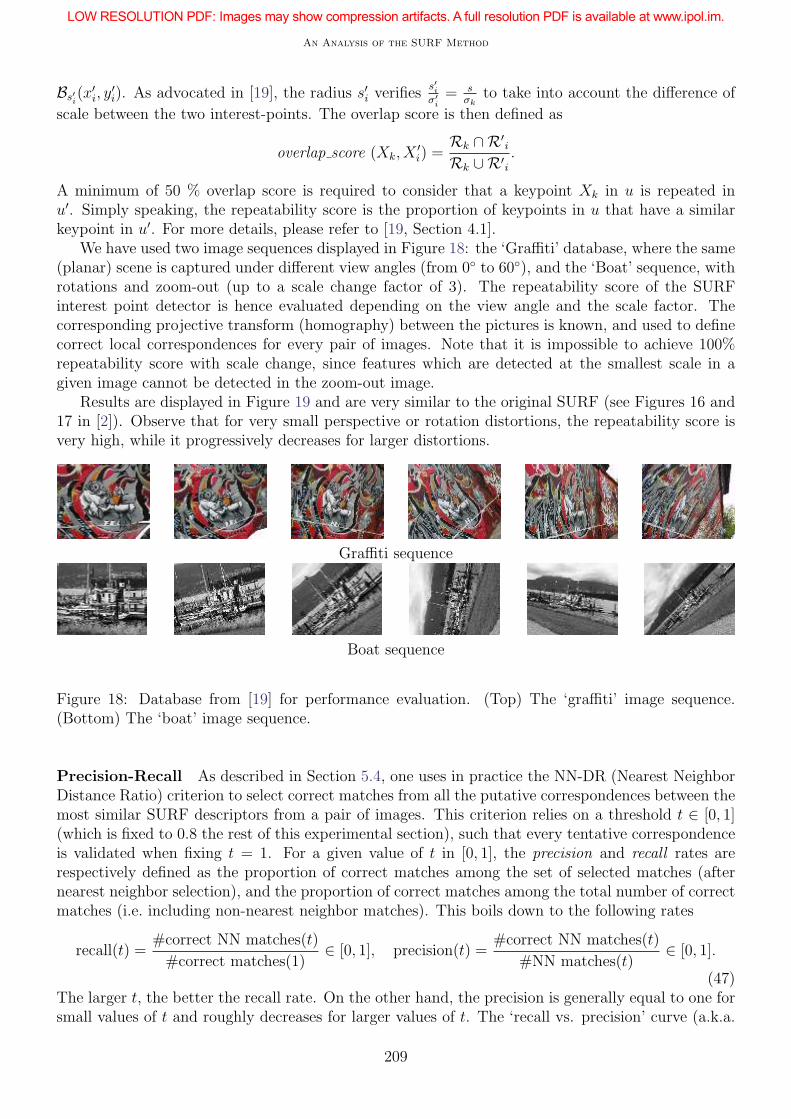
We have used two image sequences displayed in Figure 18: the ‘Graffiti’ database, where the same(planar) scene is captured under different view angles (from 0 to 60), and the ‘Boat’ sequence, withrotations and zoom-out (up to a scale change factor of 3). The repeatability score of the SURFinterest point detector is hence evaluated depending on the view angle and the scale factor. Thecorresponding projective transform (homography) between the pictures is known, and used to definecorrect local correspondences for every pair of images. Note that it is impossible to achieve 100%repeatability score with scale change, since features which are detected at the smallest scale in agiven image cannot be detected in the zoom-out image.
Results are displayed in Figure 19 and are very similar to the original SURF (see Figures 16 and17 in [2]). Observe that for very small perspective or rotation distortions, the repeatability score isvery high, while it progressively decreases for larger distortions.
Graffiti sequence
Boat sequence
Figure 18: Database from [19] for performance evaluation. (Top) The ‘graffiti’ image sequence.(Bottom) The ‘boat’ image sequence.
Precision-Recall As described in Section 5.4, one uses in practice the NN-DR (Nearest NeighborDistance Ratio) criterion to select correct matches from all the putative correspondences between themost similar SURF descriptors from a pair of images. This criterion relies on a threshold t ∈ [0, 1](which is fixed to 0.8 the rest of this experimental section), such that every tentative correspondenceis validated when fixing t = 1. For a given value of t in [0, 1], the precision and recall rates arerespectively defined as the proportion of correct matches among the set of selected matches (afternearest neighbor selection), and the proportion of correct matches among the total number of correctmatches (i.e. including non-nearest neighbor matches). This boils down to the following rates
recall(t) =#correct NN matches(t)
#correct matches(1)∈ [0, 1], precision(t) =
#correct NN matches(t)
#NN matches(t)∈ [0, 1].
(47)The larger t, the better the recall rate. On the other hand, the precision is generally equal to one forsmall values of t and roughly decreases for larger values of t. The ‘recall vs. precision’ curve (a.k.a.
209

Edouard Oyallon, Julien Rabin
20 30 40 50 600
20
40
60
80
100
View point
Repeata
bili
ty %
Repeatability for graffiti
1 1.5 2 2.5 30
20
40
60
80
100
Repeata
bili
ty %
Scale change
Repeatability for boat
Figure 19: Evaluation of repeatability detection on the datasets displayed in Figure 18. (Left) usingthe ‘graffiti’ image database, and (Right) using the ‘boat’ image database.
ROC curve) is hence built to illustrate this trade-off between recall and precision rate when tuningthe parameter t.
The precision-recall curve for the ‘Boat’ database is displayed in Figure 20. More precisely, weused the images #1 and #3 of the sequence displayed in Figure 18. Let us observe that the recallrate is in practice strictly lower than 1 since we only consider nearest neighbor matches. When t = 1,the recall rate indicates the proportion of matches that are correct, which is here around 50%. Incomparison, using random assignment between N = 103 interest points would give in average a recallrate of approximately 1
N= 0.1%.
0 0.1 0.2 0.3 0.4 0.5 0.6 0.7 0.8 0.9 10
0.1
0.2
0.3
0.4
0.5
0.6
0.7
0.8
0.9
1
1−precision
reca
ll
precision & recall
Figure 20: Precision-recall curve for the ‘Boat’ image pair (using image #1 and #3).
210
An Analysis of the SURF Method
6.2 Comparison with SIFT Approach
As previously mentioned, the SURF method shares a lot of common features with the SIFT ap-proach [15]. For a complete, in-depth analysis, we refer the reader to [24]. Some of the theoreticalaspects of multi-scale analysis have been already discussed in this Section 3. Let us recall that SIFTdetects features using multi-scale Gaussian derivatives and then builds similarity invariant descriptorsbased on local histograms of gradient’s orientation. On the other hand, SURF uses fast second orderbox filters for interest point detection and then computes first order gradient statistics to encodelocal information.
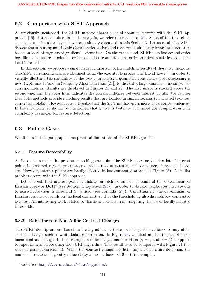
In this section, we propose a small visual comparison of the matching results of these two methods.The SIFT correspondences are obtained using the executable program of David Lowe 4. In order tovisually illustrate the suitability of the two approaches, a geometric consistency post-processing isused (Optimized Random Sampling Algorithm from [21]) to discard a large amount of incompatiblecorrespondences. Results are displayed in Figures 21 and 22. The first image is stacked above thesecond one, and the color lines indicates the correspondences between interest points. We can seethat both methods provide matching results that are located in similar regions (contrasted textures,corners and blobs). However, it is noticeable that the SIFT method gives more dense correspondences.In the meantime, it should be mentioned that SURF is faster to run, since the computation timecomplexity is smaller for feature detection.
6.3 Failure Cases
We discuss in this paragraph some practical limitations of the SURF algorithm.
6.3.1 Feature Detectability
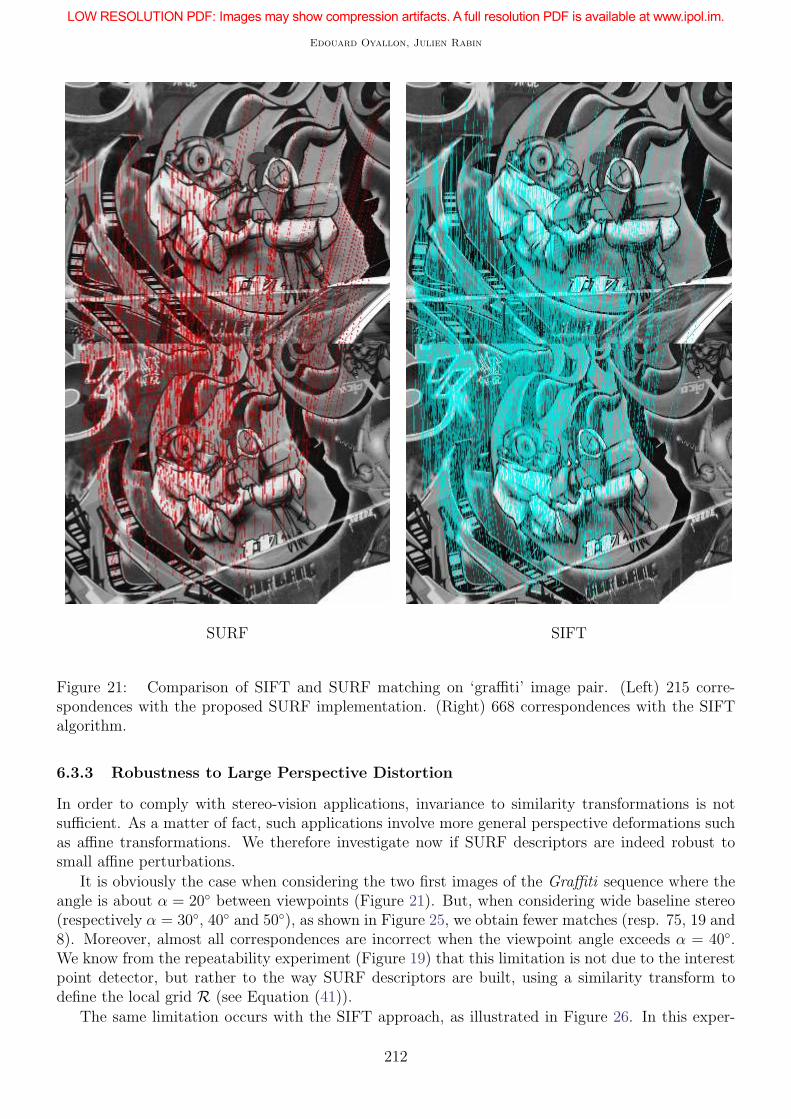
As it can be seen in the previous matching examples, the SURF detector yields a lot of interestpoints in textured regions or contrasted geometrical structures, such as corners, junctions, blobs,etc. However, interest points are hardly selected in low contrasted areas (see Figure 23). A similarproblem occurs with the SIFT approach.
Let us recall that interest point candidates are defined as local maxima of the determinant ofHessian operator DoHL (see Section 4, Equation (24)). In order to discard candidates that are dueto noise fluctuation, a threshold tH is used (see Formula (27)). Unfortunately, the determinant ofHessian response depends on the local contrast, so that the thresholding also discards low contrastedfeatures. An interesting work related to this issue consists in investigating the use of locally adaptedthresholds.
6.3.2 Robustness to Non-Affine Contrast Changes
The SURF descriptors are based on local gradient statistics, which yield invariance to any affinecontrast change, such as white balance correction. In Figure 24, we illustrate the impact of a nonlinear contrast change. In this example, a different gamma correction (γ = 1
2and γ = 4) is applied
to input images before using the SURF algorithm. This result is to be compared with Figure 21 (i.e.without gamma correction). While the contrast change has little impact on feature detection, thenumber of matches is greatly reduced (by almost a factor of 6 in this example).
4available at http://www.cs.ubc.ca/~lowe/keypoints/.
211
Edouard Oyallon, Julien Rabin
SURF SIFT
Figure 21: Comparison of SIFT and SURF matching on ‘graffiti’ image pair. (Left) 215 corre-spondences with the proposed SURF implementation. (Right) 668 correspondences with the SIFTalgorithm.
6.3.3 Robustness to Large Perspective Distortion
In order to comply with stereo-vision applications, invariance to similarity transformations is notsufficient. As a matter of fact, such applications involve more general perspective deformations suchas affine transformations. We therefore investigate now if SURF descriptors are indeed robust tosmall affine perturbations.
It is obviously the case when considering the two first images of the Graffiti sequence where theangle is about α = 20 between viewpoints (Figure 21). But, when considering wide baseline stereo(respectively α = 30, 40 and 50), as shown in Figure 25, we obtain fewer matches (resp. 75, 19 and8). Moreover, almost all correspondences are incorrect when the viewpoint angle exceeds α = 40.We know from the repeatability experiment (Figure 19) that this limitation is not due to the interestpoint detector, but rather to the way SURF descriptors are built, using a similarity transform todefine the local grid R (see Equation (41)).
The same limitation occurs with the SIFT approach, as illustrated in Figure 26. In this exper-
212

An Analysis of the SURF Method
SURF SIFT
Figure 22: Comparison of SIFT and SURF matching on ‘boat’ image pair. (Left) 289 corre-spondences with the proposed SURF implementation. (Right) 1433 correspondences with the SIFTalgorithm.
iment, it is interesting to observe that most of the correspondences found by SURF and SIFT arelocated in the less distorted area of the second image. In comparison, the ASIFT technique [28]-which is designed to tackle this kind of problem- manages to find 915 correspondences.
7 Conclusion
In this article, we have analyzed in detail the SURF [2] algorithm for local, compact and invariantrepresentation of natural images. This method achieves a performance comparable to other state-of-the-art algorithms in image matching, such as SIFT [15], while being very fast. Its use is thereforeof great interest for computer vision.
The numerical performance of the proposed implementation of SURF is consistent with thatreported in [2], but also with other implementations, such as [3].
213
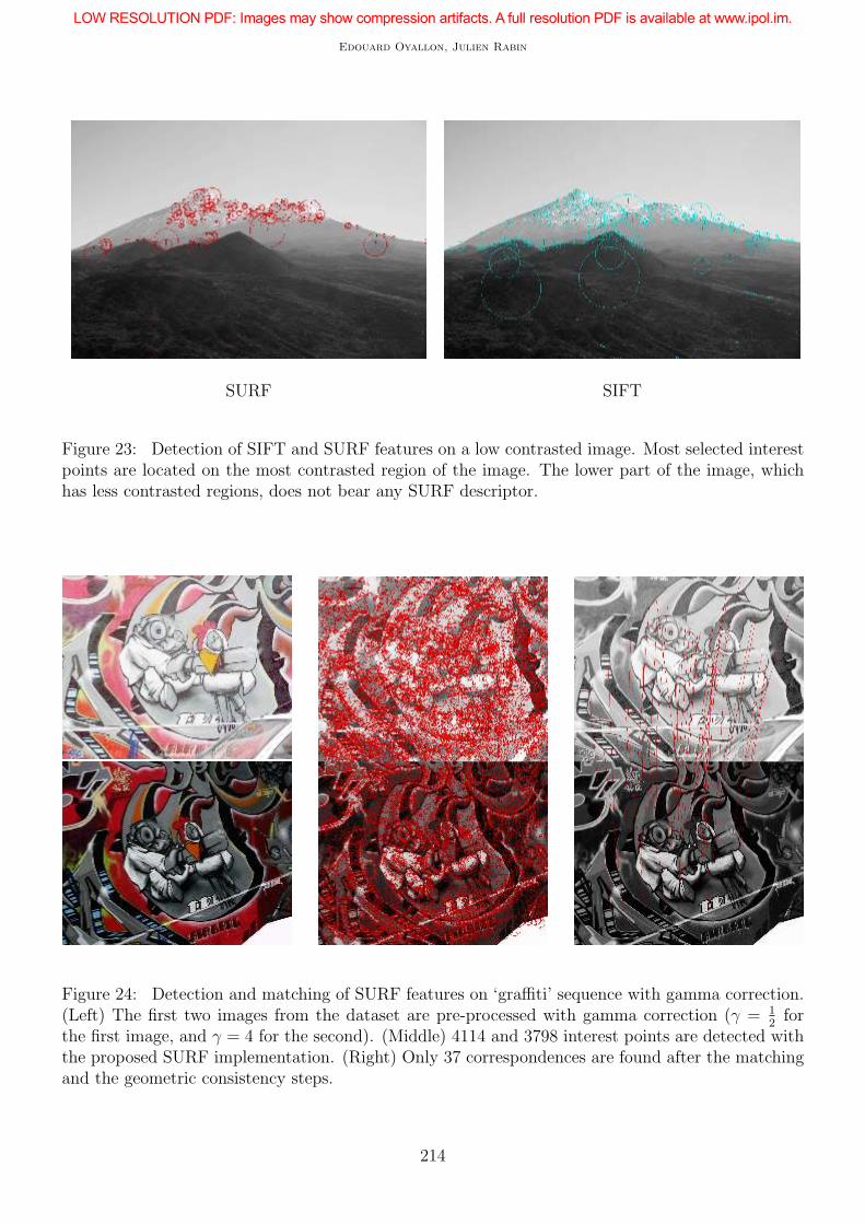
Edouard Oyallon, Julien Rabin
SURF SIFT
Figure 23: Detection of SIFT and SURF features on a low contrasted image. Most selected interestpoints are located on the most contrasted region of the image. The lower part of the image, whichhas less contrasted regions, does not bear any SURF descriptor.
Figure 24: Detection and matching of SURF features on ‘graffiti’ sequence with gamma correction.(Left) The first two images from the dataset are pre-processed with gamma correction (γ = 1
2for
the first image, and γ = 4 for the second). (Middle) 4114 and 3798 interest points are detected withthe proposed SURF implementation. (Right) Only 37 correspondences are found after the matchingand the geometric consistency steps.
214
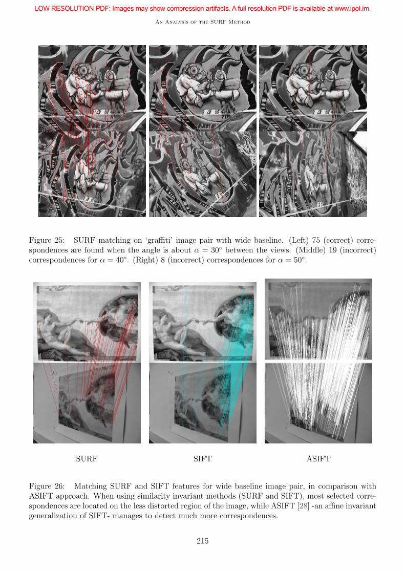
An Analysis of the SURF Method
Figure 25: SURF matching on ‘graffiti’ image pair with wide baseline. (Left) 75 (correct) corre-spondences are found when the angle is about α = 30 between the views. (Middle) 19 (incorrect)correspondences for α = 40. (Right) 8 (incorrect) correspondences for α = 50.
SURF SIFT ASIFT
Figure 26: Matching SURF and SIFT features for wide baseline image pair, in comparison withASIFT approach. When using similarity invariant methods (SURF and SIFT), most selected corre-spondences are located on the less distorted region of the image, while ASIFT [28] -an affine invariantgeneralization of SIFT- manages to detect much more correspondences.
215

Edouard Oyallon, Julien Rabin
Image Credits
, from the K. Mikolajczyk standard database
Berkeley Segmentation Dataset5
provided by the authors
Test image used in 6
Standard test image
Acknowledgments
This work was supported by the European Research Council (Advanced Grant “Twelve Labours”).The authors would like also to thank Loıc Simon and anonymous reviewers for their valuable com-ments and their suggested improvements.
References
[1] H. Bay, From wide-baseline point and line correspondences to 3D, ETH Zurich, 2009. http:
//dx.doi.org/10.3929/ethz-a-005212689.
[2] H. Bay, A. Ess, T. Tuytelaars, and L. Van Gool, Speeded-up robust features (SURF),Computer Vision and Image Understanding, 110 (2008), pp. 346–359. http://dx.doi.org/10.1016/j.cviu.2007.09.014.
[3] G. Bradski and A. Kaehler, Learning OpenCV: Computer vision with the OpenCV library,O’Reilly Media, 2008. ISBN:978-0-596-51613-0.
[4] M. Brown and D.G. Lowe, Invariant features from interest point groups, in British MachineVision Conference, Cardiff, Wales, vol. 21, 2002, pp. 656–665. http://dx.doi.org/10.5244/
C.16.23.
[5] C. Evans, Notes on the OpenSURF library, University of Bristol, Tech. Rep. CSTR-09-001,January, (2009).
[6] M.A. Fischler and R.C. Bolles, Random sample consensus: A paradigm for model fit-ting with applications to image analysis and automated cartography, Communications ACM, 24(1981), pp. 381–395. http://dx.doi.org/10.1145/358669.358692.
[7] P. Getreuer, A Survey of Gaussian Convolution Algorithms, Image Processing On Line, 3(2013), pp. 286–310. http://dx.doi.org/10.5201/ipol.2013.87.
[8] P. Gwosdek, S. Grewenig, A. Bruhn, and J. Weickert, Theoretical foundations ofGaussian convolution by extended box filtering, Scale Space and Variational Methods in Com-puter Vision, (2012), pp. 447–458. http://dx.doi.org/10.1007/978-3-642-24785-9_38.
5http://www.eecs.berkeley.edu/Research/Projects/CS/vision/grouping/segbench/6http://www.ipol.im/pub/art/2011/my-asift/
216
An Analysis of the SURF Method
[9] C. Harris and M. Stephens, A combined corner and edge detector, in Alvey vision confer-ence, vol. 15, Manchester, UK, 1988, p. 50.
[10] T. Lindeberg, Scale-space for discrete signals, IEEE Transactions on Pattern Analysis andMachine Intelligence, 12 (1990), pp. 234–254. http://dx.doi.org/10.1109/34.49051.
[11] , Scale-space behaviour of local extrema and blobs, Journal of Mathematical Imaging andVision, 1 (1992), pp. 65–99. http://dx.doi.org/10.1007/BF00135225.
[12] , Scale-Space Theory in Computer Vision, Springer, 1993. http://dx.doi.org/10.1007/
978-1-4757-6465-9.
[13] , Feature detection with automatic scale selection, International Journal of Computer Vision,30 (1998), pp. 79–116. http://dx.doi.org/10.1023/A:1008045108935.
[14] D.G. Lowe, Object recognition from local scale-invariant features, in Proceedings of the In-ternational Conference on Computer Vision, vol. 2 of ICCV ’99, Washington, DC, USA, 1999,IEEE Computer Society, pp. 1150–1157. http://dx.doi.org/10.1109/ICCV.1999.790410.
[15] , Distinctive image features from scale-invariant keypoints, International Journal of Com-puter Vision, 60 (2004), pp. 91–110. http://dx.doi.org/10.1023/B:VISI.0000029664.
99615.94.
[16] S. Mallat, A wavelet tour of signal processing, Academic press, 1999. ISBN:0123743702,9780123743701.
[17] K. Mikolajczyk and C. Schmid, An affine invariant interest point detector, in Com-puter Vision—ECCV 2002, Springer, 2002, pp. 128–142. http://dx.doi.org/10.1007/
3-540-47969-4_9.
[18] , Scale & affine invariant interest point detectors, International Journal of Computer Vision,60 (2004), pp. 63–86. http://dx.doi.org/10.1023/B:VISI.0000027790.02288.f2.
[19] K. Mikolajczyk, T. Tuytelaars, C. Schmid, A. Zisserman, J. Matas, F. Schaf-
falitzky, T. Kadir, and L.V. Gool, A comparison of affine region detectors, Inter-national Journal of Computer Vision, 65 (2005), pp. 43–72. http://dx.doi.org/10.1007/
s11263-005-3848-x.
[20] L. Moisan, P. Moulon, and P. Monasse, Automatic Homographic Registration of a Pairof Images, with A Contrario Elimination of Outliers, Image Processing On Line, 2 (2012),pp. 56–73. http://dx.doi.org/10.5201/ipol.2012.mmm-oh.
[21] L. Moisan and B. Stival, A probabilistic criterion to detect rigid point matches betweentwo images and estimate the fundamental matrix, International Journal of Computer Vision, 57(2004), pp. 201–218. http://dx.doi.org/10.1023/B:VISI.0000013094.38752.54.
[22] A. Neubeck and L. Van Gool, Efficient non-maximum suppression, in 18th InternationalConference on Pattern Recognition, vol. 3, IEEE, 2006, pp. 850–855. http://dx.doi.org/10.1109/ICPR.2006.479.
[23] J. Rabin, J. Delon, and Y. Gousseau, A contrario matching of SIFT-like descriptors, in19th International Conference on Pattern Recognition, IEEE, 2008, pp. 1–4. http://dx.doi.
org/10.1109/ICPR.2008.4761371.
217
Edouard Oyallon, Julien Rabin
[24] I. Rey Otero and M. Delbracio, Anatomy of the SIFT Method, Image Processing On Line,4 (2014), pp. 370–396. http://dx.doi.org/10.5201/ipol.2014.82.
[25] P.Y. Simard, L. Bottou, P. Haffner, and Y. Le Cun, Boxlets: a fast convolutionalgorithm for signal processing and neural networks, Advances in Neural Information ProcessingSystems, (1999), pp. 571–577. ISBN:0-262-11245-0.
[26] E. Tola, V. Lepetit, and P. Fua, Daisy: An efficient dense descriptor applied to wide-baseline stereo, IEEE Transactions on Pattern Analysis and Machine Intelligence, 32 (2010),pp. 815–830. http://dx.doi.org/10.1109/TPAMI.2009.77.
[27] P. Viola and M. Jones, Rapid object detection using a boosted cascade of simple features,in Proceedings of the IEEE Computer Society Conference, vol. 1, 2001, pp. I–511–I–518 vol.1.http://dx.doi.org/10.1109/CVPR.2001.990517.
[28] G. Yu and J.-M. Morel, ASIFT: an algorithm for fully affine invariant comparison, ImageProcessing On Line, 2011 (2011). http://dx.doi.org/10.5201/ipol.2011.my-asift.
218