an analysis of pedestrian signalization in suburban...
TRANSCRIPT

Southwest Region University Transportation Center
An Analysis of Pedestrian Signalization in Suburban A,reas
SWUTC/99/472840-00065-1
Center for Transportation Research University of Texas at Austin
3208 Red River, Suite 200 Austin, Texas 78705-2650

Tedmleal Report Doemnentation Pat!e 1. Report No.
SVVlTfCY99/4728~00065-1 I 2. Oovenunent Accession No. 3. Recipient's Catalog No.
4. Title and Subtitle
AN ANALYSIS OF PEDESTRIAN SIGNALIZATION IN SUBURBAN AREAS
S. R.Cport Date
August 1999 6. Performing Organization Code
7. Author(s)
Stephanie C. Otis and Randy B. Machemehl
9. Pert'ormiDg Oqpnization Name and Address
Center for Transportation Research The University of Texas at Austin 3208 Red River, Suite 200 Austin, Texas 78705-2650
12. SponsoriDg Apacy Name and Address
Southwest Region University Transportation Center Texas Transportation Institute The Texas A&M University System College Station, Texas 77843-3135
IS. Supplementary Notes
8. Performing Organization Report No.
10. Work Unit No. (TRAIS)
11. Contract or Gtant No.
DTOS95-G-0006
13. Type of Report and Period Covered
14. SponsoringAgeucyCode
Supported by a grant from the U.S. Department of Transportation, University Transportation Centers Program 16. AhsIract
Previous pedestrian signalization research indicated that pedestrian signals provide limited benefits to either pedestrians or vehicles. Furthermore, most pedestrian research is concentrated on downtown or high density areas, thus neglecting suburban environments. Many of these studies have used a very focused approach limiting the scope to one criterion. Without considering the full range of implications of the complex pedestrianism phenomena around signalized intersections, it is difticult to examine the delay and safety differences between pedestrians and vehicles.
This research proposes an integrated model using a mathematicaVstatistical approach. Since delay, safety, and behavior concepts have different units, they cannot be directly compared; hence, they are assessed using a costlbenefit approach. Outputs from the models produced an overall answer on pedestrian signalization benefits. Inputs were based on non-complex, readily available, and useful variables such as traffic, geometric, and land use characteristics surrounding signalized intersections. From this formulation, the question of delay and safety differences and sensitivities is addressed.
This solution approach consists of four components. A delay procedure formulates fixed and actuated delay for pedestrian and vehicular traffic. A behavior procedure determines pedestrian compliance and other measures responsive to pedestrian and vehicular traffic and signals. A safety procedure assesses pedestrian interactions with vehicular traffic. A pedestrian generation rate procedure determines the number of pedestrians crossing at a signalized intersection based on land use categorizations. The solution is tested with sample suburban scenarios and with data generated from the traffic system in Austin, Texas.
17. Key Words 18. Dislribution Sta:tement
Pedestrian Signalization, Vehicular Delay Mode~ Pedestrian Generation Rate, Pedestrian Traffic, Pedestrian Compliance, Pedestrian Signal Model, Potential Accident Rate (PAR)
No Restrictions. This document is available to the public through NTIS:
19. SeauityCJassi£(ofthisreport)
Unclassified Form DOT F 1700.7 (8-72)
National Technical Infonnation SeIVice 5285 Port Royal Road Springfield. Virginia 22161
1
20. Security CJassi£(ofthis page) 21. No. of Pages
Unclassified 134 Reproduction of completed page authorized
I 22. Priee

AN ANALYSIS OF PEDESTRIAN SIGNALIZATION IN SUBURBAN AREAS
By
Stephanie C. Otis
and
Randy B. Machemehl
Research Report SWUTC/99/472840-00065-1
Southwest Region University Transportation Center Center for Transportation Research The University of Texas at Austin
3208 Red River, Suite 200 Austin, TX 78705-2650
August 1999

DISCLAIMER
The contents of this report reflect the views of the authors, who are responsible for the facts and the accuracy of the information presented herein. This document is disseminated under the sponsorship of the Department of Transportation, University Transportation Centers Program in the interest of information exchange. The U.S. Government assumes no liability for the contents or use thereof.
u

ABSTRACT
Previous pedestrian signalization research indicated that pedestrian signals provide limited benefits to either pedestrians or vehicles. Furthermore, most pedestrian research is concentrated on downtown or high density areas, thus neglecting suburban environments. Many of these studies have used a very focused approach limiting the scope to one criterion. Without considering the full range of implications of the complex pedestrianism phenomena around signalized intersections, it is difficult to examine the delay and safety differences between pedestrians and vehicles.
This research proposes an integrated model using a mathematical/statistical approach. Since delay, safety, and behavior concepts have different units, they cannot be directly compared; hence, they are assessed using a costibenefit approach. Outputs from the models produced an overall answer on pedestrian signalization benefits. Inputs were based on non-complex, readily available, and useful variables such as traffic, geometric, and land use characteristics surrounding signalized intersections. From this formulation, the question of delay and safety differences and sensitivities is addressed.
This solution approach consists of four components. A delay procedure formulates fixed and actuated delay for pedestrian and vehicular traffic. A behavior procedure determines pedestrian compliance and other measures responsive to pedestrian and vehicular traffic
iii
ACKNOWLEDGMENTS
The authors recognize that support was provided by a grant from the U.S. Department of Transportation, University Transportation Centers Program to the Southwest Region University Transportation Center.
IV

EXECUTIVE SUMMARY
Previous pedestrian signalization research indicated that pedestrian signals provide limited benefits to either pedestrians or high-density areas, thus neglecting suburban environments. Many of these studies used a very focused approach limiting the scope to one criterion. Without considering the full range of implications of the complex pedestrianism phenomena around signalized intersections, it is difficult to examine the delay and safety differences between pedestrians and vehicles.
This research proposes an integrated model using a mathematical/statistical approach. Since delay, safety, and behavior concepts have different units, they cannot be directly compared; hence, they are assessed using a costlbenefit approach. Outputs from the models produced an overall answer on pedestrian signalization benefits. Inputs were based on non-complex, readily available, and useful variables such as traffic, geometric, and land use characteristics surrounding signalized intersections. From this formulation, the question of delay and safety differences and sensitivities is addressed.
This solution approach consists of four components. A delay procedure formulates fixed and actuated delay for pedestrian and vehicular traffic. A behavior procedure determines pedestrian compliance and other measures responsive to pedestrian and vehicular traffic and signals. A safety procedure assesses pedestrian interactions with vehicular traffic. A pedestrian generation rate procedure determines the number of pedestrian crossing at a signalized intersection based on land use categorizations. The solution is tested with sample suburban scenarios and with data generated from the traffic system in Austin, Texas.
The integrated model's general results showed that vehicular delay predominated even when pedestrian safety & delay, and equipment costs were significant. This effect caused fixed timing schemes to be costly when pedestrian timing requirements were greater than optimal vehicular signal cycle timings. When vehicular delay was unaffected, pedestrian signalization showed some promise in increasing compliance on wider streets and with higher volumes on adjoining streets. Thus, outcomes showed that pedestrian signals are most likely to be beneficial when the peak and non-peak volume patterns are similar (e.g. pedestrian and vehicular peak hours occur simultaneously). By using the convenient method of land use categorization to predict pedestrian volume at signalized intersections, these patterns can be found and the benefits of pedestrian signalization can be realized.
v

TABLE OF CONTENTS
CHAPTER 1: INTRODUCTION PROBLEM STATEMENT 1 MOTIV ATION 2 SCOPE AND OBJECTIVES OF THE STUDY 3 STUDY OVERVIEW 5
CHAPTER 2: REVIEW OF PEDESTRIAN LITERATURE INTRODUCTION 7 SAFETY 7 BEHAVIOR 9 VEHICULAR DELAY 11 PEDESTRIAN GENERATION RATES 14 SUMMARY 15
CHAPTER 3: MODELING FRAMEWORK INTRODUCTION 17 CONCEPTUAL MODEL DEVELOPMENT 17 OBJECTIVE FUNCTION OVERVIEW 18 POTENTIAL MODEL INPUTS OVERVIEW 20 MODEL OUTPUT OVERVIEW 23 SUMMARY 25
CHAPTER 4: MODELING THEORY INTRODUCTION 29 PEDESTRIAN-INDUCED VEHICULAR DELAY 29
Introduction 29 Vehicular Delay Model 30 Pedestrian Signalization Effect 37
Comparison of Pedestrian-Induced Vehicular Delay Under Different Control Strategies 39
Cost Estimates of Delays and Traffic Control Equipment 46 Summary 48
PEDESTRIAN SAFETY AND BEHAVIOR ANALYSES 48 Introduction 48 Overview of Potential Accident Rate Theory 49 Potential Accident Rate Model - Pedestrian Aspect 58 Vehicular Component of PAR Zones 59 Pedestrian Volume During Signal Phase 62 Hazard Associated with Turning Movements 64 Cost Estimates for Conflicts 68 Summary ~
VI

PEDESTRIAN DELAY 70 Introduction 70 Pedestrian Delay 70 Summary 72
PEDESTRIAN GENERATION RATES 73 Introduction 73 Pedestrian Generation Rate Theory 73 Classification Scheme 78 Summary 82
SUMMARY 82
CHAPTER 5: MODELING RESULTS 83 INTRODUCTION 83 PEDESTRIAN GENERATION RATE 83
Introduction 83 Application of Data Collection Methodology 83 Preliminary Statistics 86 Results of Pedestrian Generation Rate Regression Analyses 91
SAFETY AND BEHAVIOR ANALYSES 94 Behavior Analysis 94 Results of Logit Modeling of Compliance Rates 95 Potential Accident Rate (PAR) Trends 103
SCENARIO ANALYSIS FOR SUBURBAN AREAS 105 SUMMARY 108
CHAPTER 6: CONCLUSIONS AND RECOMMENDATIONS 111 APPENDIX 115 REFERENCES 119
vii

LIST OF FIGURES
FIGURE
3.1 Conceptual Model Development
3.2 Modified Conceptual Model Development
4.1.1 Graphical Interpretation of Queue Length Q(t) and Delay Wet)
4.1.2 Cycle Failure Analysis for 400 vph
4.1.3 Cycle Failure Analysis for 200 vph
4.1.4 Admissible Ranges of Green Intervals
4.1.5 Overview of Pedestrian-Induced Vehicular Delay Model
4.1.6 Minimum Vehicular Flows over which Pedestrian Green Times
PAGE
17
26
31
36
37
39
41
do not Govern 42
4.1.7 Percentage Delay Savings of Pedestrian Actuated Compared to Pretimed Pedestrian Signals for a 2x2 Intersection with: QlIS1=0.35 Q2/S2=0.15 43
4.1.8 Variation of Percentage Vehicular Delay Increase with N 1 and N2 44
4.1.9 Variation of Percentage Vehicular Delay Increase with Q lIS 1 and Q2/S2
4.2.1a Time-Space Concept of Potential Accident Rate Theory Signal with Green Light on Major Street
4.2.1 b Time-Space Concept of Potential Accident Rate Theory Signal with Green Light on Minor Street
4.2.2 Time-Space Concept of Conflict Theory Signal with Green Light on Major Street
4.2.3 Example Scenarios of Pedestrian Crossings of 2-Phase Cycle
4.2.4 Four Possible Cases of Compliant and Non-Compliant Pedestrians Crossing Against the Red
viii
45
50
50
51
52
54

4.2.5a Pedestrian Signal Model of General Pedestrian Crossing Choice Behavior Conditioned and Unconditioned on Phase of Arrival with General Expected Vehicular Signal Phasing 56
4.2.5b Vehicular Signal Model of General Pedestrian Crossing Choice Behavior Conditioned and Unconditioned on Phase of Arrival with General Expected Vehicular Signal Phasing 57
4.3.1a Pedestrian Delay Expectation Model due to Vehicular and Pedestrian Signals 71
4.3.1b Pedestrian Delay Expectation Model due to Vehicular Signals Only 72
4.4.1 Definition Development of Pedestrian Generation Rate
4.4.2 Typical Intersection Layout with Labeled Comers
4.4.3 Zonal Demarcation of Land Use at the Intersection
4.4.4 A Case Study: Minor Retail in the Quarter-Mile Zone and Commercial Land Use in the One-Mile Zone
5.1.1 Inter-Scorer Data Reliability Procedure
5.1.2 Average 15-Minute Pedestrian Volumes by Quarter Mile Land Use
5.1.3 Average 15-Minute Pedestrian Volumes by One-Mile Land Use
5.1.4 Average 15-Minute Pedestrian Volume over all Land Use
5.1.5 Average Hourly Pedestrian Volume over all Land Use
5.1.6 Average Hourly Pedestrian Volumes by Quarter-Mile Land Use
5.1.7 Average Hourly Pedestrian Volumes by One-Mile Land Use
IX
74
76
80
85
88
88
89
89
90
90

LIST OF TABLES
TABLE PAGE
4.1.1 Summary of Annualized Cost of Pedestrian Actuated Indications 47
4.2.1 Hazard Indexes from Knoblauch et al. (1984) 66
4.2.2 Modified Hazard lndexes 67
4.2.3 Modified Hazard Indexes to be used in Models 67
4.2.4 General Pedestrian Accident Costs 68
4.4.1 Land Use Types for Zones 1 and 2 80
5.1.1 Distribution of lntersections by Land Use 84
5.1.2 Models for Pedestrian Generation Rates 92
5.1.3 Pedestrian Generation Rate for Land Use Combinations 93
5.2.1 Arrivals and Crossings at Signalized and Unsignalized lntersections 94
5.2.2 Logit Model for Pedestrians Arriving on Steady Don't Walk and Choosing Walk over Steady Don't Walk 99
5.2.3 Example Logit Model Results for Pedestrians Arriving on Steady Don't Walk and Choosing Walk over Steady Don't Walk 103
5.2.4 Base Case Specifications 104
5.3.1 Base Case Costs 106
5.3.2 Desirable·Land Use Combinations for Actuated Signals 108
x

CHAPTER 1. INTRODUCTION
PROBLEM STATEMENT
Pedestrianism is becoming more popular due to growing
concerns for energy efficient transportation, time-space mobility
constraints and environmental pollution. In the past 50 years, cities
have become more suburban, with sprawling land-use and the
increasing need for automobiles. In addition, with increased vehicle
miles traveled per trip and congestion, drivers are more prone to stress
on the roadway and are increasingly tending to behave irresponsibly
and aggressively, otherwise known as "road rage." Combined with
pedestrianism, the consequences can be fatal. This mixture is ever so
more present at signalized intersections where pedestrians and vehicles often have conflicting movements and needs.
A traffic control strategy that deals with this problem is
pedestrian signalization. However, most research in dealing with
traffic control system design is based upon significant vehicular and
pedestrian traffic as found in central business districts (CBD). Research of pedestrian signalization in suburban environments is essentially
neglected.
Past studies noted that pedestrian signals have inherent
problems as pedestrians do not completely comply with them. Even though demand-responsive systems such as push-buttons are provided, it appears they are not completely trusted. Zegeer et al. (1982) found that installation of pedestrian Signals and crosswalk markings
may create a false sense of safety. Most pedestrian studies have focused on CBD intersections, where compliance characteristics may differ from
those in suburban environments.
Another concern is the question of the operation of pedestrian
and vehicular signals which affect delays, safety factors and other costs

between pedestrian and vehicular traffic. Currently, the operation of pedestrian signals, especially the timing issue, is governed primarily by
vehicular traffic. Compliance with signals is, however, dependent on
these factors, all of which affect pedestrian safety.
Although pedestrian accidents are a rare occurrence relative to
vehicular accidents (IIHS, 1991), the severe loss inflicted by these
accidents is the compelling reason to study the phenomena and
develop solution techniques. Characterization and understanding of
pedestrian safety with respect to behavior at intersections, signalized
and unsignalized, can enable more effective signal operation and allow
further development and evaluation of pedestrian and vehicular
control strategies. Therefore, there is a need to improve the underlying
characteristics of the interaction between pedestrian behavior and the
traffic control system.
MOTIVATION
Traffic control systems provide a variety of capabilities for
improving travel quality; however, only limited evaluations of
tradeoffs among different transportation modes have been performed.
One of the major reasons is that the variety of transportation modes prevent thorough tradeoff investigations.
Across the nation, researchers are developing new traffic control technologies for improving commuter travel quality. A primary concern is the minimization of unnecessary delay through information dispersion and other related techniques. At present, many
researchers are studying the allocation of delay among vehicular traffic
streams or paths. Researchers have recognized, however, that it is not
"vehicular delay" that must be reduced, but rather, it is "person delay."
In that sense, the process must include pedestrians.
A particular issue that has not been examined is delay, safety,
and cost allocation between vehicle users and pedestrians. There are
2

two questions that must be addressed: (1) What are the differences
between these two user classes? and (2) What is the sensitivity of delay
and safety to different traffic and geometric conditions? A framework
which allows this examination must be developed. These issues are
the primary motivation for this proposed research and understanding
them will allow inclusion of pedestrian as well as vehicular delay in
traffic control strategy design.
SCOPE AND OBJECTIVES OF THE STUDY
The goal of the proposed work is to develop an integrated model
to assess delay, safety, and behavior (i.e. compliance) in a single
framework for a suburban setting. Reaching this goal entails fulfilling
the following objectives:
1) Develop a delay model for assessing pedestrian and vehicular
delay to include compliance/safety information.
2) Characterize mathematical functions for pedestrian compliance/
safety based upon typical suburban traffic patterns.
3) Test different traffic control strategies using alternative scenarios.
4) Determine the impact suburban environment has on pedestrian/
vehicular system.
The integrated and combinatorial nature of the signalized intersection problem precludes solutions by exact optimization models. Newell (1989) developed a vehicular delay approach that included the
following two features: 1) development of vehicular delay expressions, and 2) examination of these expressions under different vehicular
traffic conditions. In addition, expressions developed by Webster offers
practical equations for usage. These models are applicable to many
different traffic control strategies.
3

In this study, the above heuristic approach is extended and
further developed to include pedestrian delay and safety concepts
oriented toward the kind of land use and traffic patterns found at traffic
signalized intersections in most suburban U.s. cities. These concepts
are tested under several different control strategies, namely fixed or
actuated vehicular signals with no, fixed, or actuated pedestrian signals.
With such an integrated framework, future pedestrian/vehicular
traffic control concepts can be tested with minor computational
changes and data requirements.
This framework differs from existing approaches in the
following aspects:
1. Ability to assess differences between pedestrian and vehicular
traffic incorporating pedestrian compliance, delay and safety
and vehicular delay. This framework also identifies optimal
control strategies for different traffic conditions.
2. Inclusion of a methodology for assessing pedestrian-induced
vehicular delay for traffic Signalization under different
pedestrian signalization schemes.
3. Characterization of pedestrian safety/compliance functions
which are integrated into the pedestrian and vehicular delay
model and interpreted as functions of traffic conditions. 4. Development of a methodology for data collection enabling
examination of both pedestrian generation rate of a suburban
environment and compliance using video, on-site and
geographic information.
5. Examination of pedestrian generation rates based upon
suburban land use to provide an efficient way of determining
pedestrian volume impact at suburban intersections. Also,
these rates are analyzed for their time-dependent nature of
4

peak hour(s), non-peak hour(s), and no-volume hour(s) of
pedestrian traffic.
In addition, the solution approach allows different weights to be
assigned to pedestrian and vehicular streams for analyzing different
scenarios.
STUDY OVERVIEW
This chapter described the significance of pedestrian
signalization in the context of its general problem and defines research
objectives and general approach.
Chapter 2 presents an in-depth literature review of various
published pedestrian studies, namely safety, behavior, vehicular delay,
and pedestrian generation rates.
Chapter 3 presents an overview of the analytical research
framework. It basically describes framework elements for pedestrian
/vehicular delay, pedestrian safety / compliance (and pedestrian
volumes) for general modeling. Framework elements are described at
an abstract level, including the objective function, its inputs and
outputs.
Chapter 4 presents the theoretical development of the vehicular·
delay framework, pedestrian safety/compliance functions, and
pedestrian generation rate analyses. The vehicular delay framework
evaluates the trade-offs between the conflicting needs of pedestrian and
vehicular traffic. The framework allows estimation of pedestrian
induced vehicular delay, and assessment of relative merits of different
pedestrian accommodation strategies. In addition, costs behind the
delays are presented.
The pedestrian safety/compliance functions in Chapter 4 are
integrated into the delay framework. Two factors, compliance and
5

potential accident rates, are developed for different traffic conditions,
namely number of lanes, vehicle volume, and traffic control type.
The pedestrian generation rate theory development is presented
in Chapter 4, containing two components: 1) the definition
development of pedestrian generation rate, and 2) the determination of
peak-hour and non-peak hour pedestrian generation rates. In addition,
a dual land use methodology for the pedestrian generation rate
analyses is described.
Chapter 5 presents results from application of the theories
presented in Chapter 4, namely, the pedestrian generation rate
analyses, the compliance rates and their resulting pedestrian safety
functions, and finally, the aggregated results from all components
integrated into benefit/cost answers. The pedestrian generation rate
analyses are performed first by examining volume patterns over time
and land use, and then by developing regression models to determine
peak and non-peak hour rates. Results from the pedestrian
compliance/safety section will state the implications of the answers
obtained, especially with respect to the traffic conditions. Finally, the
aggregated methodology will be tested for reasonableness through
sensitivity analysis, and the delay differences will be examined through different traffic/ geometric conditions and compliance rates.
Chapter 6 presents conclusions from the research results and discusses directions for future research.
6
CHAPTER 2. REVIEW OF PEDESTRIAN LITERATURE
INTRODUCTION
Researchers have taken different approaches analyzing various
aspects of pedestrianism. They have devised means of quantifying
safety, delay, and behavior based on traditional engineering analyses.
The literature reviewed can be grouped under four headings:
i) Safety
ii) Behavior (Le. compliance)
iii) Vehicular Delay
iv) Pedestrian Generation Rates
While there are many descriptive pedestrian studies, few
fundamentally quantitative investigations are available. Furthermore,
most studies focus on single behavior, safety, or signal operations
issues rather than a comprehensive assessment. This chapter presents
a general overview of these essentially conventional pedestrian
studies.
SAFETY
Characterization of pedestrian safety is an ongoing research
opportunity for which parameter definitions, coding, practicality, accuracy, and effectiveness remain problematic. Different researchers
have tried different methods with mixed results, and this section generally describes these efforts, starting with the number of accidents as a pedestrian safety indicator.
Accident frequency is a measure of safety problems, and can be
used to identify accident causes. One often quoted study using
pedestrian accident data to study safety impacts of pedestrian signals
was made by Fleig and Duffy (1967). However, their limited sample
size did not allow conclusive statistical analysis. Robertson and Carter
7

(1984b) used existing state data bases and found that approximately one
of every five vehicles involved in an intersection accident was turning
with left-turning vehicles being more predominant. Also, they found
that the young and the elderly are more accident susceptible. In
addition, Robertson (1984a) found that left turns are almost three times
more hazardous to pedestrians than through movements, and he
quoted other studies that found after implementation of Right-Turn
on-Red, pedestrian accidents increased. Another study (Zegeer et al.,
1982) provided evidence using accident data to show that pedestrian
signalized intersections are no safer than unsignalized intersections.
Witkowski (1988) studied the relationship between land-use type and
accident rates. He concluded that intersection-related accidents more
often occur in areas of commercial or financial land-use, and
residential land-use is more frequently associated with mid-block
accidents. Zaidel and Hocherman (1988) used accident rates to compare
performance of pedestrian crossing arrangements. A general drawback
of the accident analysis approach is that accidents are rare phenomena,
and not all are reported. They occur under various circumstances
making identification of generic causes difficult. Some researchers
have felt that development of site-specific remedies is easier; hence, it
is the usual practice.
Since accidents are rare and available databases are not extensive,
researchers attempted to substitute conflict data for accident data. A
conflict occurs when pedestrians and vehicles "nearly" come into
contact with each other causing one and/or the other to change a
course of action (Cynecki, 1980; Davis et aL, 1989). Conflicts can be
obtained from road-side observations. Cynecki (1980) identified
thirteen different types of conflicts and defined a conflict severity index
to reflect the degree of hazard at the intersection. The index is obtained
for different sites and compared to identify risky intersections. This
approach requires observers to undergo rigorous training so that an
8

acceptable degree of observational uniformity can be obtained. Garder
(1982) also used this technique to relate conflict and accident data.
The conflict technique is more effective than the accident
analysis approach at developing intersection-specific remedies. The
disadvantage of this method is that site-specific deficiencies; therefore,
identification of general causes may not be possible. In other words,
this method may not allow safety (or lack of) to be related to
geometric/traffic conditions. Pedestrian and/or driver movements,
which is the primary precursor to an accident or a conflict, has not been
directly addressed.
Another method for predicting accident rates is the use of
exposure measures (indicators of pedestrian and vehicle volume).
Knoblauch (1984) has shown that exposure measures yield high hazard
scores for certain groups such as the young and elderly, those running,
crossing against the red, outside the intersection area, and/or where
buses and motorcycles exist. This same study also pointed out that
there is considerably less hazard with left or right turning vehicles
except in the case of right-turn-on-red. Unfortunately, the conflict and
exposure studies have shown mixed results (i.e. conflicting information) when tested against accident rates.
Within the conflicting results, there were a number of consistent
findings, especially when geometric/traffic variables were used.
However, this paradox indicates that a different approach is needed for characterizing and evaluating pedestrian safety at signalized intersections. The factors must be analyzed and a different safety
concept should be introduced.
BEHAVIOR
Pedestrian crossing behavior is defined as the phenomena
surrounding decisions/movements for crossing streets at signalized
intersections. Of particular importance is the decision when to cross
9

the intersection, or in other words, when they decide to comply or not
comply with traffic/pedestrian signals. Compliance rates are affected by
many factors for which a general overview is provided in this section.
Mortimer (1973) compared compliance rates at intersections with
and without pedestrian signals, and concluded that signalized
intersections experience higher compliance. However, the installation
of these signals has not always proven effective. Zegeer et al. (1982)
found that there was no difference in accident frequency between pre
timed intersections with and without pedestrian signals. Lack of
understanding and uniformity of these signals could be one reason for
their ineffectiveness. Another reason could be that pedestrians signals
do not change the cycle lengths; hence, pedestrians might feel that they
are insufficiently served. One study (Bailey et al., 1991) on the elderly
reports that sixty-four percent of the respondents lacked adequate signal
phase understanding. Also, most avoided crossing during peak hours
and at low visibility periods. Studies of young pedestrians show that
they have very unsafe attitudes concerning street crossing. As with
people who are not familiar with pedestrian signals, children need to
be provided with safe-crossing information and to be convinced that
they are valuable tools.
Signal timing also has an impact on compliance. A study by
Robertson and Carter (1984b) reports that when too much green was
given to the vehicular traffic relative to its volume, pedestrian
violations increased. Also, they found that longer pedestrian clearance
time increased the number of violations. Khasnabis et al. (1982), in
their review of behavior studies, observed that (i) at low vehicle
volumes, pedestrians are likely to ignore signal indications, (ii)
compliance rate for steady "walk" is higher than flashing "walk", and
(iii) pedestrian clearance intervals increase compliance rates.
Another result obtained from characterizing pedestrian crossings
comes from gap acceptance theory. Palamarthy (1993) modeled
10

pedestrians' gap acceptance behavior under different scenarios using a
multinomial probit approach. Estimation results pointed to trends on
gap acceptance and push-button behavior. On the gap acceptance
behavior at busy or wide intersections, these gap acceptance values are
higher, people are less cautious while crossing on turn phases, and
group interactions are significant and should not be ignored. On the
push-button behavior, people may have an inherent tendency to avoid
using push buttons, but at busy or wide intersections, push buttons
might be of some assistance to the pedestrians.
Although choice models are preferable to simple statistical
correlation of compliance with geometric/traffic variables, using gap
acceptance parameters as independent variables is difficult. Relating
gap acceptance parameters to geometric/traffic parameters is difficult
and mixing other parameter types and providing specific numerical
results to crossing choice phenomena is highly problematic. In this
sense, choice modeling using geometric/traffic parameters directly
appears to be a preferable methodology.
VEHICULAR DELAY
For determining pedestrian impacts on vehicular traffic, most
researchers have used statistics. Many have not mathematically
modeled the crossing phenomenon, though some efforts have been
assisted by simulation. In this section, these efforts are reviewed.
Although researchers have studied both vehicular and
pedestrian delay, more emphasis has been given to vehicular delay.
Robertson (1984b) studied pedestrian and vehicle delay at signalized
intersections, which is a function of signal timing, pedestrian and
vehicle volumes, and roadway width. Usually overlooked, pedestrian
compliance with the signal can have a significant effect on pedestrian
delay. Pedestrian compliance is usually greater when vehicle volumes
are high. When vehicle volumes are low, or when too much green is
11

given to vehicles, pedestrians tend not to comply. Those who trust
their own judgments and cross before their own time usually decrease
their own delay.
King (1977) used pedestrian delay as a principal traffic signal
warrant criterion, primarily for traffic conditions under which
adequate gaps may never occur. The rationale for the pedestrian
warrant was that it should be based on an acceptable level of average
pedestrian delay, a tolerable level of maximum delay, and an equitable
total delay allocation. His study found that at vehicular saturation
rates, the average pedestrian delay without signals was higher than the
average vehicular delay with Signals. The delay equity criterion was
ultimately dropped even though he stated that pedestrians are less comfortable standing than drivers (and passengers) sitting inside
vehicles. A major study (Griffiths et aL, 1984a, b, & c, 1985) completed on
pedestrian and vehicular delay, used observations of 215,000 vehicles
and 75,000 pedestrians to develop a simulation program. A
mathematical model was developed using simple queuing
relationships. Vehicular delay described in this model is in the form of
total delay per vehicle as pedestrian (and vehicle) volumes increase, not in terms of the increase due to pedestrian signal impact.
Abrams and Smith (1977a & b) discussed the practicality of using phasing schemes other than the combined pedestrian-vehicle interval.
Three alternatives studied were early release, late release and scramble timing. These alternatives determined when all or right-turning only
vehicles are allowed to proceed. The early release alternative allowed
pedestrians to cross before right-turning vehicles could proceed, and
vice versa for the late release alternative. Scramble timing is also
called "exclusive timing" because a phase for pedestrians only (for all
crosswalks) is provided. These alternatives were evaluated in terms of
pedestrian and vehicle delay and safety. The data collection included
12

vehicle delay, pedestrian generation rates, pedestrian delay, and
pedestrian compliance. Vehicle delay was defined as the difference
between time required for right-turning vehicles with and without
pedestrians.
Compared to standard timing, early release timing caused no
additional pedestrian delay for higher pedestrian volumes. Higher
vehicular delay occurred at lower pedestrian volumes and higher
vehicle volumes. This phasing will always result in additional total
person-delay.
Compared to standard timing, late release timing causes more
pedestrian delay if pedestrian volume is high. For high vehicle
volumes, more vehicular delay occurred, and for concurrently high
pedestrian levels, the vehicular delay results were mixed. Compared to
standard timing, scramble timing causes the pedestrian delays to
increase for both parallel and diagonal crosswalks. In most cases,
standard pedestrian phasing minimizes total intersection delay. This
appears to be particularly true for low pedestrian volumes. Newell's (1989) examination of traffic signal timings includes
extensive discussions on vehicular delay and includes occasional
discussions on the effect of pedestrians on vehicular delay. Most
discussions dealing with pedestrians are qualitative rather than
quantitative. Moreover, Newell's approach to quantifying traffic signal expressions allows researchers to change parameters to incorporate new ideas, try different approaches, and to effectively analyze the outcome without resorting to overly extensive efforts. In this case, his
approach should be used and extended to evaluate pedestrian-induced
vehicular delay and examine trade-offs underlying signal operation
strategies.
13

PEDESTRIAN GENERATION RATES
Pedestrian volumes have generally been the major variables for
determining when pedestrian signals should be installed.
Traditionally, the number of pedestrians has been obtained through
field counting. In addition, methods for predicting pedestrian volumes
using secondary data have been concentrated in CBD areas or other
relatively high density areas. These studies are described in this
section.
Expressions predicting pedestrian volume characteristics based
only on short volume counts were developed (Seneviratne et aL, 1990a
& b, Hocherman et al., 1988). A similar study in Israel examined CBD
and residential areas (Hocherman et al., 1988), but recommended the
developed models only be used with similar sites, and additional
counts would be needed to attain transferability. Sandrock (1988) suggested land use should be considered as a predictor variable.
Another CBD study attempted to explain pedestrian volumes
using land-use types and quantities as predictor variables (Behnam, 1977); however, the results are not transferable because geographic
characteristics were not taken into account. A more detailed CBD study
related walking distance, trip generation rates, and volume variation to available walkway space and building space (Pushkarev et al., 1971). One-third mile was the average walking distance, and half of all pedestrians walked less than 1,000 feet.
A study in Washington D.C. used land use as the principal site selection criterion (Davis et aL, 1988). Mathematical models which use
short volume counts as predictor variables were developed, and the
authors claimed that the models worked well, although wondered
about transferability. A major limitation of this study is that only sites
with "significant pedestrian volumes" were chosen and all were in
well developed Washington D.C. areas.
14
A promising variable is land use surrounding the site.
However, since land use in relation to pedestrian traffic in suburban
areas has not been studied extensively, an examination of land use
impact on pedestrian traffic in suburban areas is needed.
SUMMARY
This chapter discussed and assessed the literature relevant to
pedestrian safety and behavior, vehicular delay, and pedestrian
generation rates. The findings reveal that research is needed in
modeling pedestrian crossing phenomena. Results from other studies
show promise in models using geometric/traffic variables.
In addition, these findings point out that very little effort has
been concentrated on pedestrian behavior in suburban environments.
Although many similarities to CBD areas are expected, certain
characteristics, including pedestrian volumes and vehicular speeds are
different and these are expected to affect pedestrian behavioral
responses.
These findings provide a focus for the next chapter which
discusses the general framewor k for the conceptual and
methodological approach to address the concerns.
15

16

CHAPTER 3. MODELING FRAMEWORK
INTRODUCTION
This chapter presents an overview of the analytical research
framework It describes the previously identified components, namely
pedestrian/vehicular delay, pedestrian safety / compliance (and
pedestrian volumes) for the general modeling framework Framework
elements are described at an abstract level, including the objective
function, inputs and outputs.
CONCEPTUAL MODEL DEVELOPMENT
Figure 3.1 illustrates the conceptual model development flow.
Results Sensitivity Analysis
Figure 3.1 Conceptual Model Development
All elements in the shaded area except solution techniques are
described briefly in this chapter. The objective function is stated, and a
discussion of the units is described. The range of possible modeling
inputs are briefly described; then, preselected primary inputs are
identified. The complexity of the output units that affects the objective
17
function is descri~ed, and a unit-output solution is presented. In
addition, a brief discussion on intermediate model outputs is described;
the purpose of these output types is to examine statistical trends behind
pedestrian crossings.
The solution technique is described in Chapter 4 theoretical
modeling efforts. The results, sensitivity analysis, and assumption
modifications are presented in Chapter 5. The major results use the
objective function presented in the next section.
OBJECTIVE FUNCTION OVERVIEW
Traffic control strategies are usually implemented expecting
several benefits. One major potential benefit is accident reduction and
the other is user delay minimization. At traffic-signalized
intersections, the decision to implement pedestrian control devices
depends upon these pedestrian delay and safety benefits, and vehicular
delay and hardware costs for the given traffic/geometric scenario.
Ideally, all direct costs should be minimized and all direct benefits
maximized. Such an objective function would be very difficult to
solve, if not impossible. For this research, all units were converted to
costs which were transformed to monetary benefits, and thus, all benefits, direct and indirect (e.g. proxy variables), are maximized.
Monetary benefits of pedestrian signalization are expected to
vary over time, especially as pedestrian/vehicle volumes change.
Many cost/benefit studies compute annual costs because the
information needed is available. However, because of lack of
information regarding many pedestrian traffic characteristics,
particularly pedestrian volumes, this research focuses on costs/benefits
on a typical day.
Since intersections under study already have basic vehicular
signal equipment, it is necessary only to determine the
18
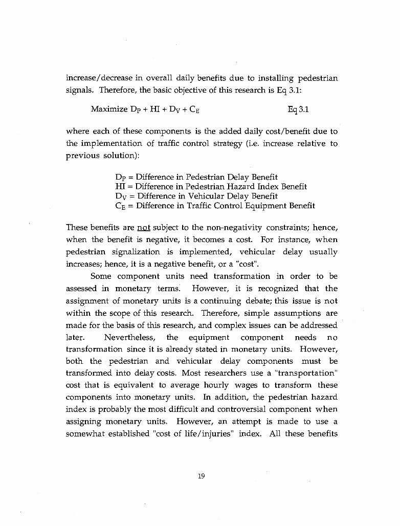
increase/ decrease in overall daily benefits due to installing pedestrian
signals. Therefore, the basic objective of this research is Eq 3.1:
Maximize Dp + HI + Dy + CE Eq3.1
where each of these components is the added daily cost/benefit due to
the implementation of traffic control strategy (i.e. increase relative to
previous solution):
Dp = Difference in Pedestrian Delay Benefit HI = Difference in Pedestrian Hazard Index Benefit Dy ::: Difference in Vehicular Delay Benefit CE = Difference in Traffic Control Equipment Benefit
These benefits are not subject to the non-negativity constraints; hence,
when the benefit is negative, it becomes a cost. For instance, when
pedestrian signalization is implemented, vehicular delay usually
increases; hence, it is a negative benefit, or a "cost".
Some component units need transformation in order to be
assessed in monetary terms. However, it is recognized that the
assignment of monetary units is a continuing debate; this issue is not
within the scope of this research. Therefore, simple assumptions are
made for the basis of this research, and complex issues can be addressed
later. Nevertheless, the equipment component needs no transformation since it is already stated in monetary units. However, both the pedestrian and vehicular delay components must be transformed into delay costs. Most researchers use a "transportation" cost that is equivalent to average hourly wages to transform these
components into monetary units. In addition, the pedestrian hazard
index is probably the most difficult and controversial component when
assigning monetary units. However, an attempt is made to use a
somewhat established "cost of life/injuries" index. All these benefits
19

except pedestrian hazard index are explained in detail in Section 4.1.4;
the pedestrian hazard index is explained in Section 4.2.
POTENTIAL MODEL INPUTS OVERVIEW
A comprehensive modeling approach to predicting pedestrian
signalization benefits might include all factors affecting benefits.
However, benefits vary due to many factors including, geometrics,
control type, human behavior, traffic conditions, and environmental
elements. In addition to research studies from the previous section
indicating the complexity of pedestrian signal phenomena, Robertson
et al. (1984b) lists many factors that control pedestrian Signal benefits. A
main portion of this section describes some of these factors indicating
the complexity of deciding which factors to include in analyses.
Geometric factors include median islands, lighting, parking,
street width, and sight distance. Median islands vary in width from
three to more than twenty feet and may encourage noncompliance.
Lighting can become an issue for those who have sight impairments
such as the elderly. Parking is often a critical visibility issue for
children who cannot see above parked cars and a parking lane adds
roadway width. Sight distance is often blocked by shrubbery, is sometimes obscured by roadway geometries, and made diffieult with certain signal placements.
Control factors include vehicle signals, pedestrian signals,
pedestrian push buttons, phasing, and timing. Vehicle signals include
fixed-time, actuated, and coordinated; each of which may produce
different effects upon pedestrians in terms of delays and predictability
of vehicle movements. Pedestrian signals include fixed-time and
pedestrian-actuated. Fixed-time signals have cyclically occurring
pedestrian phases whereas pedestrian-actuated signals display
pedestrian indications only when called, potentially reducing vehicular
delay. Both signal types have many different compliance consequences
20
under many different situations. Pedestrian push buttons allow
pedestrians to declare their need for a pedestrian phase; however,
people have different reactions toward this device. The phasing (of
vehicles) can be difficult in the sense that pedestrians may not be able
to predict the phase sequence and/ or understand the phasing
indications. In addition, the phase timing may be too short (or too
long) for different pedestrians. Crosswalks have also been used for
pedestrians albeit with questionable concerns.
Human factors include age, gender, physical disability;. walking
speed, compliance, risk-taking, gap acceptance, group behavior, erratic
behavior, comprehension, and accidents. The young (under 14), and
the elderly (over 60) may have difficulty understanding the rules and
technology of traffic signals. Gender may be an issue if in certain
geographic areas, gender may be correlated with traits such as vigilance
or aggressiveness or with level of education. Physical disability is often
a concern in three areas: the blind, deaf, or mobility-impaired. Audible
signals are under intense debate among the visually-impaired
community, experts and advocacy groups concerned with blindness
issues. The deaf may not hear vehicles approaching or stopping. The
mobility-impaired not only would have difficulty in crossing at a
normal pace, but might have difficulty getting on and off sidewalks
that do not comply with ADA requirements. Walking speeds vary greatly, especially for the elderly, young, and mobility-impaired. Compliance rates vary usually with vehicle volumes and other site characteristics; if pedestrians do not comply with the signal indications,
then its benefits are questionable. Risk-taking and erratic behavior
usually are exhibited by younger pedestrians, uneducated pedestrians
and rushed pedestrians. Gap acceptance is the process by which
pedestrians decide to cross between passing vehicles, and it varies by gender, age, and other factors. Group dynamics may influence difficult
crossing behavior; for instance, if one person crosses the street
21

prematurely, others may follow without fully assessing the situation.
Young pedestrians, rural pedestrians (who may not be familiar with urban traffic control), and elderly pedestrians may lack traffic signal
knowledge.
Traffic factors include vehicle volume, pedestrian volume,
vehicle speed, vehicle mix, vehicle directional split, vehicle delay, pedestrian delay, vehicle arrivals, pedestrian crossings, and gap
distribution. Higher vehicle and pedestrian volumes, and vehicle
speed and mix usually increase accident probabilities. Vehicle
directional split may confuse pedestrians. Pedestrian delay increases reduce signal compliance rates. Vehicle arrival patterns may influence
pedestrian signal phasing and pedestrian crossing patterns could dictate the type of pedestrian signal. If there are large but few pedestrian groups, then pedestrian-actuated signals may be very beneficial.
Environmental factors include weather, time of day, pollution,
and energy considerations. In storm conditions, vision may be
impaired, and vehicular movements may be more erratic, leading to more hazards. Also, snow conditions may prevent pedestrians from
crossing in a timely manner. Night-time conditions may be more
difficult for vehicle drivers to detect pedestrians. Also, those with vision problems may find nighttime more difficult.
A framework which considers all factors would be nearly incomprehensible. Therefore, only those factors that have general importance and/or can be controlled are considered. As concluded from the literature review chapter, a primary focus in this research should be on geometric/traffic factors. Since many factors interrelate to ,
many others on many different levels (e.g. vehicular signal timings are influenced by vehicle volumes, saturation flow rates, and other
variables), the primary inputs to these models are listed here. In later
chapters, the interrelations are described more fully. From this
standpoint, the primary input variables are vehicle volumes, speed,
22

saturation flow rates and number of lanes. In addition, to account for
individual pedestrian characteristics, pedestrian volumes, walk speed,
start-up time, and compliance are included. A total of eight input
factors have been preselected. These factors along with several other
input factors are tested and assessed in Chapter 5. Major and
intermediate outputs from this model using these inputs are described
next.
MODEL OUTPUT OVERVIEW
Model output is a recommendation on whether or not to install
pedestrian signals. Units used for the outcome are in dollars per hour.
However, as stated before, there is considerable variation of
pedestrian/vehicular traffic characteristics in a 24-hour period.
Since every traffic demand case is based upon optimized cycle
lengths, one could use 24 different hourly demand conditions of a
typical day and determine controller performance during each hour.
However, because isolated pretimed controllers generally have one, at
most three, different Signal timing plans, they cannot continuously
optimize timing. Pretimed controllers are generally optimized for one (possibly 3) design hour(s). Analysis of pre-timed vehicle signals is
limited to peak hours only, because incremental delays are relative to
optimized cycle lengths and simple pre-timed controllers are generally
optimized for one design-hour condition. Using hourly benefits the net value or benefit/cost over a 24-
hour period can be calculated if hourly information on pedestrian and
vehicle volumes is available. In most instances, average hourly
vehicle volume counts will be available, but not average hourly pedestrian volume counts.
The above methodology could be used when all 24 hours of
pedestrian and vehicular volumes are available; however, this is
usually not the case. To simplify the amount of pedestrian, as well as
23

vehicular information required, yet consider traffic and pedestrian
volume variation, a simplified approach is presented. This approach
yields a weighted net value sum with the day divided into three parts
based upon pedestrian generation rates. These three parts include
peak, non peak, and zero (or near zero) pedestrian crossings. The
number of zero pedestrian hours is based on the concept that very few
pedestrians appear at most intersections between 11 pm and 7 am; hence, HO is estimated as eight hours.
Net Value (24 hour) Hp X (Bp) + Hnp X (Bnp) + HO X (BO) where
Hp Hnp HO
Bp Bnp BO
number of hours of peak pedestrian volumes number of hours of non-peak pedestrian volumes number of hours of zero pedestrian volumes (usually 8 hours) net value during the peak pedestrian hour net value during the non-peak pedestrian volume hour net value during the zero pedestrian volume hour
Pedestrian volumes of all hours between 7 am and 11 pm are
determined using numbers from the pedestrian generation analyses
presented in Section 5.1. The theoretical framework behind pedestrian
generation rates is presented in Section 4.3.
Before the ultimate output is obtained, other types of outputs are examined not just for reasonableness, but also to gain insight on the
pedestrian crossing phenomenon. More detail will be given in Chapter 4; however a brief overview is given here.
Vehicular delay can be affected by pedestrian crossings. That is,
given certain traffic/geometric intersection characteristics, pedestrian
signalization may require greater green phase durations than provided
by vehicular indications. Preliminary outputs from Section 4.1 on
vehicular delay analyses indicate how likely this scenario is.
Concurrently, vehicular delay can be affected by pedestrian
compliance especially under pedestrian actuation. However,
pedestrian non-compliance can affect pedestrian safety; since non-
24

compliance is heavily influenced by traffic and geometric
characteristics, compliance variability is examined. The theory from
Section 4.2 explains how compliance and safety are interrelated.
How compliance affects vehicular delay is also determined by the number and manner of pedestrian crossings. Section 4.3 describes
the cause/effect of pedestrian crossing volume on the vehicular traffic stream.
Ultimately, results from Chapter 5 provide insight derived from
analyzing pedestrian impacts on vehicular traffic in the modeling and
statistical analyses. Through sensitivity analysis, combinatorial effects
of these changes are tracked.
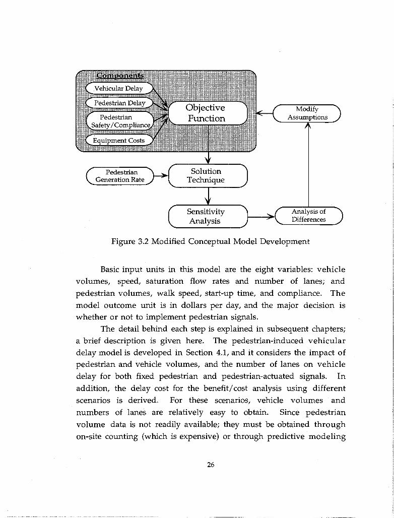
SUMMARY Figure 3.2 describes Figure 3.1 when the information from
Sections 3.2 through 3.4 are added. The delay model is developed along
with the pedestrian generation rates, pedestrian safety/compliance
functions. The outcome is subjected to sensitivity analysis and analysis
of delay differences; and the assumptions are modified when necessary.
25
Pedestrian Generation Rate
Sensitivity Analysis
Analysis of Differences
Figure 3.2 Modified Conceptual Model Development
Basic input units in this model are the eight variables: vehicle
volumes, speed, saturation flow rates and number of lanes; and
pedestrian volumes, walk speed, start-up time, and compliance. The
model outcome unit is in dollars per daYt and the major decision is whether or not to implement pedestrian signals.
The detail behind each step is explained in subsequent chapters;
a brief description is given here. The pedestrian-induced vehicular
delay model is developed in Section 4.1, and it considers the impact of pedestrian and vehicle volumes, and the number of lanes on vehicle
delay for both fixed pedestrian and pedestrian-actuated signals. In
addition, the delay cost for the benefit/cost analysis using different
scenarios is derived. For these scenarios, vehicle volumes· and
numbers of lanes are relatively easy to obtain. Since pedestrian
volume data is not readily available; they must be obtained through
on-site counting (which is expensive) or through predictive modeling
26

which is presented in Sections 4.3 and 5.1. The safety and compliance of pedestrians is modeled and analyzed in Sections 4.2 and 5.2.
The source of information for the predictive pedestrian
generation rate model, compliance and safety analyses is gathered
through on-site observation and video recording. The site selection criteria and data collection efforts are described primarily in Sections 4.3 and 5.1.
27

28
CHAPTER 4. MODELING THEORY
INTRODUCTION
The theoretical framework for assessing relative delay and safety
benefits is explained, and some effects of its implications are illustrated
in this chapter. In addition, modeling for determining intersection pedestrian volume levels is shown.
PEDESTRIAN-INDUCED VEHICULAR DELAY
Introduction
At certain intersections, pedestrians may require more time to
cross than is required to serve vehicle arrivals; therefore, if a pedestrian
signal is provided, it may cause vehicular delay. Pedestrian-signal
activation is one strategy for avoiding wasted vehicular green and
delay to vehicles. A framework is developed in this section to evaluate
the trade-offs between the conflicting needs of pedestrians and
vehicular traffic. The framework allows the estimation of pedestrian
induced vehicular delay and assessment of the relative merits of
different pedestrian accommodation strategies.
Delay times for vehicles for the three possible pedestrian
signalization conditions are examined. If there are no pedestrian
signals, vehicular traffic phase lengths are unaffected by pedestrians
(assuming pedestrian requirements are not taken into consideration in setting green times); however, pedestrians may experience delays. Fixed time or non-actuated (no push buttons) pedestrian signals may,
under light vehicle traffic conditions, force longer than optimal cycle lengths causing vehicular delays. Pedestrian actuated pedestrian signals may also force longer than optimal cycle lengths but only when
a pedestrian phase is called. Effects of these three pedestrian control
options upon fixed (pre-timed) or actuated vehicular traffic controllers
are examined.
29

This framework is developed on the basis of Webster's equations
and Newell's (1989) "Theory of Highway Traffic Signals." Fixed-time
signal timings follow Webster's equations. Since suburban
intersections frequently have low vehicle volumes, short cycles could
result from Webster's equations; hence, cycle failure analysis was
performed to determine minimum cycle lengths for all situations.
This cycle failure discussion follows the Section on Newell's theory on
vehicular-induced vehicular delay. Newell's theory is then adapted to
include the estimation of pedestrian-induced vehicular delay. Next,
numerical illustrations for typical situations allow comparisons
between signal operation for fixed pedestrian signal and pedestrian
actuated signal operation. Finally, cost estimates of delay for the 24-
hour vehicle volume variation are presented.
Vehicular Delay Model
Signal operation at an isolated intersection involves conflicting
objectives. The desired outcome is the minimization of the
"signalization cost" incurred by competing vehicular flows. However,
this cost has many possible components: travel time, stops,
environmental detriments, delay, accidents, etc. Newell explicitly
considered two of these objectives, total delay and number of stops,
each of which carries different optimal signal setting implications.
Delay minimization favors short cycle times because vehicles would
have shorter red-time waiting periods. Minimization of the number of
vehicular stops favors longer cycles because fewer vehicles would have
to stop due to fewer signal changes (and fewer occurrences of lost time
at the beginning and end of each phase). Because delay appears to be
more sensitive to the cycle time, delay minimization has generally
been the primary consideration.
This section focuses on Newell's development because of its
explanatory nature, but also describes Webster's equation used for
30

fixed-time signals. The analysis begins with a description of the
processing of vehicles through the intersection. In Figure 4.1.1, the
queue length and associated delay are illustrated. At any time at a
traffic signiil, some vehicles are stopped while others are moving. At a
time t, after the start of the effective green during which the queue is
discharging, the associated delay to a vehicle is W(t), and the queue
length is Q(t). (The effective green time for, vehicles is smaller than the
actual signal's green, because vehicles need additional time to begin to
move, and there are fewer vehicles moving through the yellow time.)
/ /
/
/
/ /
/
" Average Number of Vehicles During Green Time
Time Effective Green Time
Figure 4.1.1 (Newell, 1989): Graphical Interpretation of Queue Length Q(t) and Delay W(t).
From this simple deterministic analysis, the fraction of vehicles
that are delayed is calculated as Eq. 4.1.1.
31

where
(C - G + 't) f= C
f = fraction of vehicles that are delayed C = cycle length in seconds G = green phase length in seconds 't = effective green time in seconds
Eq.4.1.1
Since the effective green time, 't = q(C-G)/(sat-q), depends on several
variables, including vehicular and satuation flow, this equation can be
converted to exclude 't (Eq. 4.1.2).
where
f _ (l-G/C) - (l-q/sat)
q = vehicular flow in vehicles per hourI sat = saturation flow rate in vehicles per hour
Eq.4.1.2
The average delay per vehicle that "experiences" delay is taken to be
half the red time, (C-G)/2. Thus, the total average delay (Eq 4.1.3) for
all vehicles is the fraction of those delayed multiplied by the average
delay per vehicle. - 1 (GJ C
W = 2." I-C) (l-q/sat) Eq.4.1.3
where w = average delay (in seconds) per vehicle
For a four-way intersection, the total delay per unit time is equal to the
sum of the number of vehicles multiplied by the average delay per
vehicle in each direction.
An additional delay term is added to take into account variability
in the arrival and departure procedure. This delay term is used to
I"q" is used instead of nv" just for this section to follow Newell's notation
32

incorporate variability into the signal timings can be used to account
for the hourly differences in timing plans. Newell gives an extensive
discussion on the formulation of this stochastic term, Q; the form
given in Eq. 4.1.4 divided by the vehicular flow and added to the above
deterministic form presented in Eq. 4.1.3. Its main component, t is a
stochastic term used for taking into account the variance of the number
of arrivals per cycle versus the mean number of arrivals per cycle.
Q= I 2 (1 _ C (q~sat) )
where Q the stochastic term for the average queue at start of red I = the main stochastic term C = cycle length in seconds G = green phase length in seconds q = vehicular flow in vehicles per hour sat = saturation flow rate in vehicles per hour
Eq.4.1.4
Newell provides an expression for the "optimal" cycle time that
minimizes a weighted sum of delay and number of stops, and derives
expressions for the total vehicular delay per unit time and green time
for each approach given the optimal cycle CEq. 4.1.5}. Therefore, since
all of Newell's calculations are based on optimized signals, they could
be either actuated or pre-timed.
Eq.4.1.5
where L = total lost time before and after signal changes phasing in seconds Subscripts "1" and "2" refer to major and minor street, respectively
33

Webster's equation (Eq. 4.1.6) shows frequently used fixed
timed signal cycle. Its critical lane flows are based on the heaviest
vehicle volumes for each signal indication by multiplying a weight to
each turning movement.
where
1.5L+5 c=---l-:Lb i
Eq.4.1.6
L = total lost time before and after signal changes phasing in seconds bi = critical lane flow divided by saturation rate
The free time remaining after the green phase has been used to serve
q/s for both streets is split (Eq. 4.1.7) using not the q/s split as in
Webster's studies, but as the square root of "Iq/sat".
K=
where
Il(ql/satl) 12( q2/ sat2)
K = cycle split ratio used for distributing the "free time"
Eq.4.1.7
In theory, optimized signal operations under fixed traffic demand conditions yield similar performance for both traffic-actuated
signals and fixed-time traffic signals. Under variable traffic demand
conditions, traffic-actuated signals adjust to changing demand. However, the long-run average timings of ideal traffic-actuated signals would be comparable to continuously optimized timings of fixed traffic
signals. Furthermore, minimum and maximum green times of traffic
actuated signals are established using fixed or point estimates of traffic
demand. For design or peak hours, timing plans for actuated signals
generally cause loss of green through maximum extension ("max out")
for most cycles which causes performance much like fixed -time
34

controllers. Minimum cycle length causes cycle failure i.e. vehicles not
processed efficiently because the green phase is too short; this
phenomena is discussed next.
Cycle Failure
Since suburban vehicular volumes are low during most hours
of an average day, an analysis of the cycle lengths using Webster's
equation for fixed cycles was performed. The reason for these analyses
is that low vehicular volumes generally cause cycle lengths to be small,
especially 2-phase cycles, causing some cycles to be as short as 20
seconds under Webster's equation. For actuated cycles, small cycle
lengths are generally not a problem since the signal is more responsive to vehicular volume changes.
However, for fixed cycles, if the cycle length is very short, then cycle failures are likely. Cycle failure occurs when any green phase
duration of any cycle is insufficient to clear the waiting vehicle queue.
For example, if a green phase is 10 seconds, and there are 5 vehicles
queued at the beginning of the green phase which happen to require 15
seconds to move through the intersection, then possibly 2 vehicles
have to wait until the next cycle. Although cycle failures may not be avoidable during rush hours, they are highly undesirable during low
vehicular volume periods because they cause unnecessary congestion. In addition, cycle failures, if at all possible should be avoided so that
vehicle driver frustration does not lead to over-aggressive behavior. Cycle failure performance analysis was created using simulation
of vehicles arriving at the intersection in a random process and
moving through the approach taking into account lost time and saturation flow. Vehicles that arrived during the red phase, but could
not get through the intersection in the following green phase were
considered to be cycle failure victims. If the vehicles arrived during the
green phase after the waiting queue has cleared, then they are not
35

considered to be cycle failure victims. Hence, cycle failure occured only
when all available green phase time was spent processing the waiting
queue, but the initial waiting queue could not be completely served.
Since vehicular volumes of 100 to 400 vph have been noted
during non-peak hours in suburban areas, this analysis was performed
using lost times, L, (clearance intervals) between three and six seconds
and cycle lengths of 20, 30, 35, 40 and 45 seconds (with green phase
exactly half of cycle lengths). Cycle lengths of 20 seconds were generally
the outcome from Webster's cycle equation, but cycle failure
experimentation included 30, 35, 40 and 45 seconds to determine a
reasonable minimum cycle length.
From Figures 4.1.2 (400 VPH) and 4.1.3 (200 VPH), the cycle
failure percentage (over all cycles in one hour) increased dramatically
for 20-second cycle lengths compared to longer cycle lengths. The increase from 30-seconds to 35-seconds or longer· is much less
significant. For vehicular volumes of 100 or less, the results were less
dramatic.
1.0
<I) Q) l-< 0.8 ::l -.,.., «!
J;J:., Q)
0.6 ~ U --0 0.4 Q)
co «! ..... t::: Q)
0.2 ~ Q)
~
0.0 10 20 30
Cycle Length
Lost Time, L --I.if-- 3 sec
• 4 sec III! 5 sec
----¢»- 6 sec
40
Figure 4.1.2 Cycle Failure Analysis for 400 vph
36
50
0.20.,..------------------------,
(\)
!=j -~ 0.15
(\) -u >.
U 0.10
10 20 30
Cycle Length
Lost Time, L
---EJ-- 3 sec • 4 sec a 5 sec 0< 6 sec
40
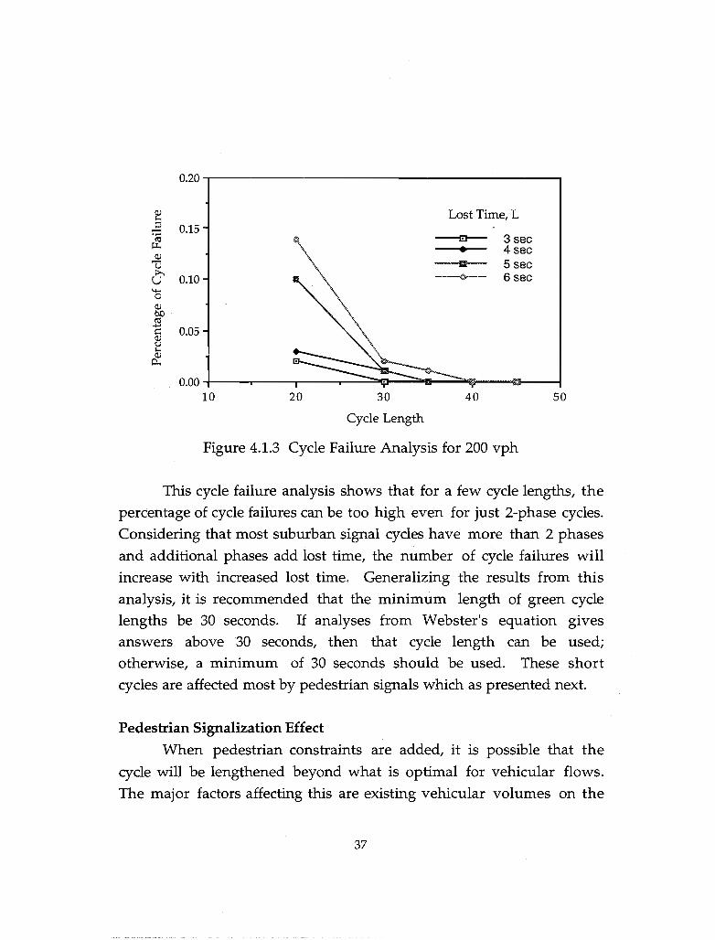
Figure 4.1.3 Cycle Failure Analysis for 200 vph
50
This cycle failure analysis shows that for a few cycle lengths, the
percentage of cycle failures can be too high even for just 2-phase cycles.
Considering that most suburban signal cycles have more than 2 phases
and additional phases add lost time, the number of cycle failures will
increase with increased lost time. Generalizing the results from this
analysis, it is recommended that the minimum length of green cycle lengths be 30 seconds. If analyses from Webster's equation gives answers above 30 seconds, then that cycle length can be used;
otherwise, a minimum of 30 seconds should be used. These short
cycles are affected most by pedestrian signals which as presented next.
Pedestrian Signalization Effect
When pedestrian constraints are added, it is possible that the
cycle will be lengthened beyond what is optimal for vehicular flows.
The major factors affecting this are existing vehicular volumes on the
37

approaches and the pedestrian crossing time requirement (a function of
street width and walking speed).
The first factor, traffic volumes, mayor may not govern the
traffic signal when there is pedestrian signalization. In other words, if
the traffic volume is large for both directions, the cycle length required
to handle the volumes will be greater than the required pedestrian
crossing time.
The second factor, the time required for a pedestrian to cross the
street consists of two parts: reaction time and physical crossing time.
The reaction time that is widely accepted by traffic engineers is 5
seconds. Although this reaction time seems long, it provides extra
time for the elderly and children. The time to cross the street depends
on the street width and the walk rate (for which a typical accepted
value of 3.5 feet per second is used for this section's illustration
purposes).
In this analysis, the traffic volume on the major street is always
at least as great as that on the minor street. If green time for the minor
street is small, the major red will be small and pedestrians may require
more time to cross the major street than that provided. In other words,
if pedestrian signalization constrains signal operation, frequently the increased cycle length will be induced by increased mirror direction green time, G2. This constraint is seen in Figure 4.1.4 at the minimum minor-street required green time, Gm 2. With this increased G2I a new
cycle length is calculated along with a new corresponding G1 value.
The relationship illustrated in Fig. 4.1.4 ensures that the new G1 also
38

-L
.... o s::: ~
Gm1
-L Major Street
~, ~ = Green Time Gm1' Gm2 = Minimum PedestrianGreen Time
L= Lost Time
Figure 4.1.4 Admissible Ranges of Green Intervals
satisfies the pedestrian minimum Gm1. The delay from pedestrian
constrained operations is calculated using the same equations discussed earlier.
Comparison of Pedestrian-Induced Vehicular Delay Under Different Control Strategies
In order to isolate the effect of pedestrians on vehicular delays,
comparisons are performed between optimized (based on vehicular
traffic) signal operation with no pedestrian signal phase as the base case
and the following two cases: (1) optimized signal with pre-timed
39

pedestrian signal system and (2) optimized with pedestrian-actuated
operation. This comparison helps in assessing the benefits of
pedestrian actuation. An overview of the procedure is presented in
Figure 4.1.5.
The following assumptions are made in this comparison for this section. First, on a street with no obstacles other than traffic signals,
ideal saturation flow rate was frequently assumed as 1800 vehicles per
hour. However, there are usually several factors which limit this
saturation rate (buses, trucks, grades, etc.); hence, a practical value of
1600 vehicles per hour was assumed. Street widths were calculated on
the basis of 12 feet per lane; even though many street lanes are
narrower than this, there is usually some additional roadway width
that pedestrians have to cross such as parking lanes, shoulders and/or
medians. Second, the variability of the arrival process on major street
approaches is assumed to be somewhat greater than on the minor
street because of the character of traffic on the major streets and overall
higher vehicular volumes.
With these assumptions, the first step in determining the effect
of pedestrian constraints is to calculate the values of the critical
vehicular flows in excess of which the pedestrian green requirements
do not govern the cycle time. This baseline set of results are shown in Figure 4.1.6.
40

Calculate C; I G:u for Vehicles
,r Calculate C; I G::! for Pedestrians
,r Calculate Vehicular Delay for No Pedestrian Signalization
,r / Calculate Impact on Vehicular Delay .......
for Actuated Pedestrian Signalization ~ith Different Pedestrian Arrival Rates..,l
,r /Calculate Percent of Time Differences .......
between No and Actuated Pedestrian Signal Control on Vehicular Delay for
'- Different Pedestrian Arrival Rates .)
Determine Pedestrian Volume for which Actuated Pedestrian
Signal Control is Beneficial
Figure 4.1.5 Overview of Pedestrian-Induced Vehicular Delay Model
41

0.8,...----.-----r---...,.-----r----r------.
:= o ~ 0.7~----_+--~--~~~~~~~~~~~~~--~ .e ~ ::s -It! en o i 0.6 .e;:::l.I.en ... -.!!!O ::s_ (.)
:c
~-----+---4~~--~~~----~~----_+----~
~ 0.5~-----+------~~~~+_--~~~----_+------~
~ -en ... . 2-~ 0.41----+----i----+-~~~-.......;~.---l -~ Pedestr an Crossi 9 Times ;: Lon er Than ptimal It! II: V hicular Ti ins
0.3~---~---~-----~---~------~----~
-e- N1=2;N2=1
-Ir- N1=2;N2=2
-II- N1=3;N2=1
-a- N1=3;N2=2
-iii- N1=3;N2::3
0.1 0.2 0.3 0.4 Ratio of Minor Street Vehicular Flow to Saturation Flow
(Q2/S2)
For 5= 1600 Q/5 Q(vphpl) 0.20 320 0.35 560 0.45 720 0.55 880
0.65 1040 0.70 1120
N1 & N2 = Number of lanes on major and minor approaches. Q1 & Q2 ::; flows on major and minor approaches. 51 & 52 ::; saturation flow rates on major and minor approaches.
Usage Note: Locate vertical and horizontal lines representing the minor and major street ratios of flow to saturation flow (Q1/51 and Q2/52). If their lines intersect below the line representing ntnnbers of traffic lanes on the two streets, then pedestrian minimum greens force longer than optimal vehicular traffic green intervals. Figure 4.1.6 Minimum Vehicular Flows over which Pedestrian Green
Times do not Govern
42

Figure 4.1.7 illustrates a case for the advantages of pedestrian
actuation over a pre-timed pedestrian signaL Clearly, the benefits are
greater for lower pedestrian flow rates (Jl).
3
B case 1 - ped-pre-timed (I) 0 case 2 ped-actuated til ('is (I) ... 0
oS >-~ (I)
c ... ('is
::::s 1 0
~ (I)
> (I) C') 1 ('is -c (I) 0 ... (I)
a.
0.0 0.5 1.0 1.5 2.0 2.5 3.0 11 (pedestrians I minute)
Figure 4.1.7 Percentage Delay Savings of Pedestrian Actuated Compared to Pretimed Pedestrian Signals for a 2 x 2 Intersection with: Ql/Sl=0.35 Q2/S2=O.15
Figure 4.1.8 illustrates the variation of percentage delay increase
caused by pre-timed pedestrian phases compared to vehicular traffic
optimized phases with the number of lanes. The wider the street,
particularly the major street, the higher the potential is for delay
savings with pedestrian-actuated signals.
43
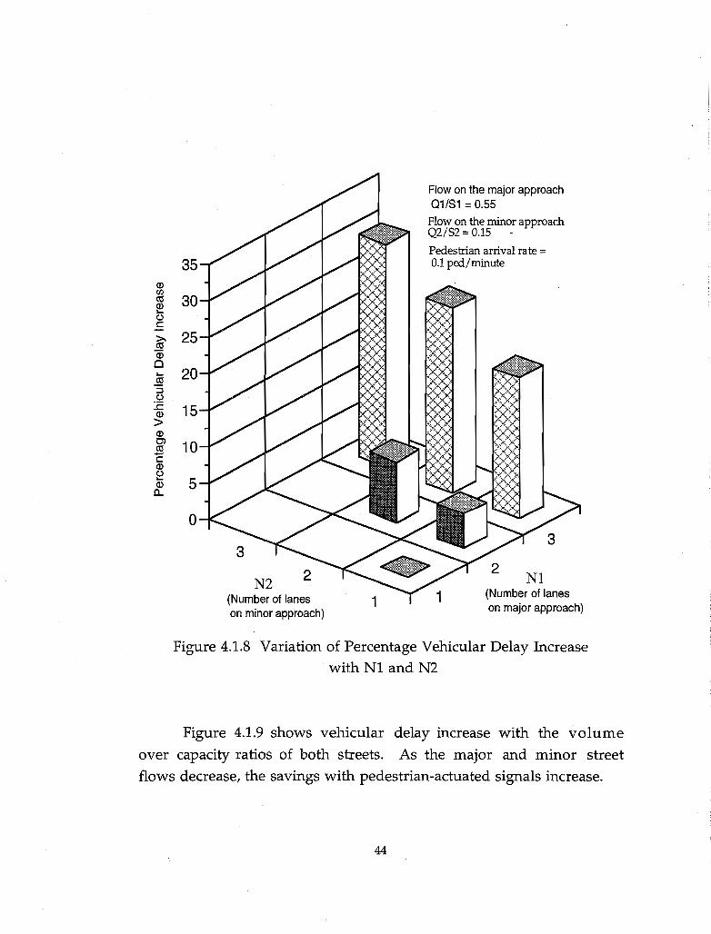
35
CD
~ 10 E CD E CD 5 0..
o
N2 (Number of lanes on minor approach)
1
Flow on the major approach Q1/81 = 0.55
Flow on the minor approach Q2/S2 = 0.15 -
Pedestrian arrival rate = 0.1 ped/minute
Nl (Number of lanes on major approach)
Figure 4.1.8 Variation of Percentage Vehicular Delay Increase with N1 and N2
Figure 4.1.9 shows vehicular delay increase with the volume
over capacity ratios of both streets. As the major and minor street
flows decrease, the savings with pedestrian-actuated signals increase.
44

Q) en m ~ 0 c:
~ Qi 0 :....
E:! ::J 0 :c: Q)
> Q) 0> m -c: Q)
e Q)
0..
20
Q1/S1 (Major approach flow)
Number of lanes on major approach N 1 ::: 2
Number of lanes on minor approach N2 ::: 2
Pedestrian arrival rate::: 0.1 ped/minute
(Minor approach flow)
Figure 4.1.9 Variation of Percentage Vehicular Delay Increase with Ql/Sl and Q2/S2
Pedestrian delays approximate the time lost when no pedestrian
signals are provided or the time saved if signals are provided. Minor
differences exist between pedestrian time saved under fixed pedestrian
phases and actuated pedestrian phases.
All calculations are based upon vehicular signal timing
optimized for each specific vehicular demand condition. As noted
earlier, under fixed traffic demands truly optimized pretimed vehicular
traffic controllers and ideal actuated controllers behave very similarly.
45

The signal timing optimization process used here included effects of
random vehicle arrivals which caused somewhat larger optimal cycle
lengths. Real actuated controller cycle lengths are constrained by minimum and maximum green times.
Cost Estimates of Delays and Traffic Control Equipment
Costs associated with pedestrian and driver times are similar to
wages, or per capita income as in many transportation studies. In
Texas, the per capita income for 1992 was $17,852 (Schlesinger Jr, 1993).
For 1993, the rate is adjusted to $19,323. As stated in Section 3.2,
assumptions are simplified for cost analysis since cost assignment is
not within this research scope. Pedestrian and drivers' values of time
are assumed equal. Since there are approximately fifty 40-working
hour-weeks per year, the cost per hour is set at $10.
Table 4.1.1 displays the estimated cost of actuated pedestrian
signals, which is the sum of the fixed pedestrian signal costs from
Robertson's study (1984) and the estimated cost of push-buttons. The addition of push-buttons is estimated to be 25% of the equipment cost
and 50% of the maintenance cost. The costs of power consumption and
push-button installation (when part of the initial installation) is assumed to be negligible. Since costs are quoted in 1981 dollars, an
inflation factor of 2.52 was used to convert to 1993 dollars2. This rate is very close to the Consumer Price Index for a similar time period. Therefore, the total 1993 annual cost per signal is approximately $350, and with eight pedestrian signals per intersection, the total cost is
$2800. This cost becomes $0.32 per hour when divided by 8760 hours
per year.
2 This conversion factor also uses a discount rate of 8%. Although current inflation and interest rates are below 8% at this time, it may increase substantially again in the future.
46
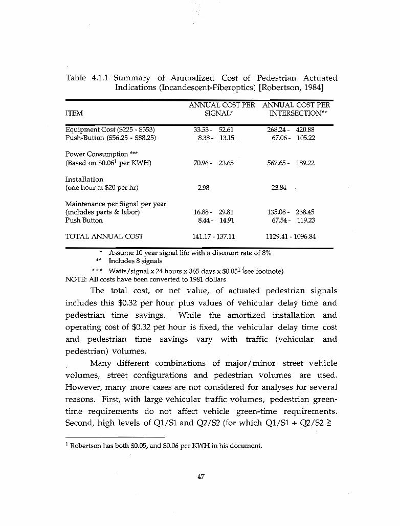
Table 4.1.1 Summary of Annualized Cost of Pedestrian Actuated Indications (Incandescent-Fiberoptics) [Robertson, 1984]
ITEM
Equipment Cost ($225 - $353) Push-Button ($56.25 - $88.25)
Power Consumption *** (Based on $0.061 per KWH)
Installation (one hour at $20 per hr)
Maintenance per Signal per year (includes parts & labor) Push Button
TOTAL ANNUAL COST
ANNUAL COST PER ANNUAL COST PER SIGNAL * INTERSECTION**
33.53 52.61 8.38 13.15
70.96 - 23.65
2.98
16.88 - 29.81 8.44- 14.91
141.17 -137.11
26824 - 420.88 67.06 - 105.22
567.65 - 189.22
23.84
135.08 - 238.45 67.54 - 119.23
1129.41 - 1096.84
* Assume 10 year signal life with a discount rate of 8% ** Includes 8 signals
* * * Watts I signal x 24 hours x 365 days x $0.051 (see footnote) NOTE: All costs have been converted to 1981 dollars
The total cost, or net value, of actuated pedestrian signals
includes this $0.32 per hour plus values of vehicular delay time and
pedestrian time savings. While the amortized installation and
operating cost of $0.32 per hour is fixed, the vehicular delay time cost and pedestrian time savings vary with traffic (vehicular and pedestrian) volumes.
Many different combinations of major/minor street vehicle volumes, street configurations and pedestrian volumes are used.
However, many more cases are not considered for analyses for several
reasons. First, with large vehicular traffic volumes, pedestrian green
time requirements do not affect vehicle green-time requirements. Second, high levels of Q1/S1 and Q2/S2 (for which Q1/S1 + Q2/S2 ~
1 Robertson has both $0.05, and $0.06 per KWH in his document.
47
0.90) present near- or over-saturated conditions. Third, very low levels of Q1/S1 and Q2/S2 (for which Q1/S1 ~ 0.15) rarely occur at signalized
intersections, except late-night or early-morning hours. If these
conditions appear, then the net value number is $-0.32 per hour.
These net values appropriately describe cases for hourly vehicular and pedestrian volumes compared to optimized traffic
signals without pedestrian indications. However, both vehicular and
pedestrian volumes change among the hours of a typical 24-hour day.
Summary
This section illustrated that with higher numbers of lanes, low
vehicular flows, and large numbers of pedestrians, pedestrian-actuated
signals exhibit potential for net economic savings. By examining the
24-hour time period, this analysis takes into account vehicle and
pedestrian volume fluctuations. With this model, the inputs are
vehicular volumes, numbers of approach lanes, and pedestrian
generation rates. The vehicular volumes and number of approach
lanes are easily obtainable while pedestrian volumes are not; therefore,
pedestrian generation rates are provided in Section 4.3. Next, the
implications of pedestrian safety in this framework are presented for which pedestrian delay is then derived from.
PEDESTRIAN SAFETY AND BEHAVIOR ANALYSES
Introduction
The effectiveness of pedestrian signals in maximizing safety (Le.
minimizing accident rates) depends on two factors: compliance and
potential accident rates. These two factors depend on several factors,
namely number of lanes, presence of median, vehicle volume,
vehicular speed, pedestrian volume, and traffic control type. The
potential accident rate is a measure of intersection safety and the
compliance rate is a measure of pedestrian behavior. This section first
48

presents an overview of the potential accident theory and then,
explains how compliance is embedded in it.
Overview of Potential Accident Rate Theory As shown in the literature review, accident rates are difficult to
analyze using observational data; hence, the concept of "potential
accidents" is developed. A modified form of the traditional conflict
theory is used.
The traditional conflict concept enumerates the number
/severity of potential vehicle and pedestrian "contacts." It is measured
by counting the number of types of close encounters between vehicles
and pedestrians. For example, a conflict occurs when a pedestrian runs
to avoid being hit. Researchers have developed models correlating
accident and conflict rates. There are four drawbacks to this traditional
concept. First, statistical relationships between conflict rates and
accident rates have not always been significant and consistent. Second,
a large conflict database is required; which means, at low pedestrian
volumes, an enormous amount of time spent acquiring data is
required to obtain reasonable statistical models. Third, even if
statistically significant results were obtainable, significant field data
quantities would be required in order to apply the model(s). Finally, it
is difficult to apply the traditional conflict theory in a theoretical
framework because it is difficult to determine how conflict rate increases are due to different geometric/traffic conditions. For
instance, given the earlier conflict example of a pedestrian running to
avoid being hit, it is nearly impossible to determine what this event's
likelihood is due to changes in vehicular volume, or this event's
likelihood differences between four- and six-lane approach streets.
A concept that overcomes these problems is the time-space
potential accident rate concept (or "PAR" for simplicity) illustrated in
Figures 4.2.1a and 4.2.1b. The boxes aligned along the crosswalk path
49

indicate when pedestrians are, or are not, free from potential vehicle
conflicts with respect to the traffic signal timing. The three boxes in
each lane of the two-lane road represent the three available vehicular
movements: left, through, and right. The four-lane road has two boxes
in each lane since left turns are not permissible from _ right lanes and
right turns are not permissible from left lanes. The marked boxes
indicate potential vehicle-pedestrian accidents whereas the unmarked
boxes signify absence. For instance, in Figure 4.2.1a, the major street
has the green light; therefore, the minor street's crosswalk has more
PAR-free zones. In Figure 4.2.1b, the situation is reversed; the minor
street has the green.
~- gg
=
Major Street~t
Minor Street \.
Figure 4.2.1a Time-Space Concept of Potential Accident Rate Theory Signal with Green Light on Major Street
~=CD~caL _~I I~_
I I 1= eBCD cal Figure 4.2.1b Time-Space Concept of Potential Accident Rate Theory
Signal with Green Light on Minor Street
50

The theory behind using different PAR zones for different
vehicular movements is that certain vehicular movements are more
hazardous to pedestrians, usually because of lack of visibility or
noncompliance. Although literature sources have indicated mixed
results regarding left/right turn movements, most hay:e indicated that
turning movements are more hazardous than straight movements.
Figures 4.2.1a & b present scenarios with permitted left turns and
right-turns-on-red (RTOR). If RTOR and/or left turns were prohibited
when pedestrian movements occurred, then the number of PAR-free
pedestrian zones increases.
In addition, walking out of crosswalks presents conflicts to
pedestrians in every signalization strategy since pedestrians are not
protected in these areas. The PAR zones can be seen in Figure 4.2.2.
Figure 4.2.2 Time-Space Concept of Conflict Theory Signal with Green Light on Major Street and Conflict Zones Outside of Crosswalk
The differences between intersections with or without
pedestrian signals and/or crosswalks in terms of PAR-free zones can be
insignificant. However, if the cost of having certain types of potential
conflicts is great, then small differences in traffic control strategies can
51
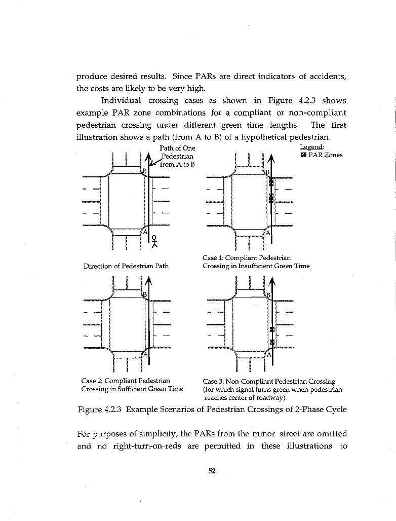
produce desired results. Since PARs are direct indicators of accidents,
the costs are likely to be very high.
Individual crossing cases as shown in Figure 4.2.3 shows
example PAR zone combinations for a compliant or non-compliant
pedestrian crossing under different green time lengths. The first
illustration shows a path (from A to B) of a hypothetical pedestrian. Path of One Legend:
Direction of Pedestrian Path
Case 2: Compliant Pedestrian Crossing in Sufficient Green Time
181 PAR Zones
Case 1: Compliant Pedestrian Crossing in Insufficient Green Time
Case 3: Non-Compliant Pedestrian Crossing (for which signal turns green when pedestrian reaches center of roadway)
Figure 4.2.3 Example Scenarios of Pedestrian Crossings of 2-Phase Cycle
For purposes of simplicity, the PARs from the minor street are omitted
and no right-turn-on-reds are permitted in these illustrations to
52

demonstrate how different green times and compliance characteristics
affect potential accidents. Case #1 shows a compliant pedestrian
provided with insufficient green time; the pedestrian will face
potential conflicts at the end of the crossing. Case #2 also shows a
compliant pedestrianf but provided with sufficient .green time; no
potential accidents will occur2. Case #3 shows a non-compliant
pedestrian; the potential accidents could occur in the beginning of the
crossing becausef in this examplef the signal turns green when the
pedestrian reaches the roadway center.
From the single pedestrian casef the multiple pedestrian case is
examined next. In Figure 4.2.4, examples of compliant and non
compliant pedestrians crossing against the red are shown. In each of
the individual crossing examples, a pedestrian is either crossing with
the green (0%) or crossing against the red (100%). The results are
dichotomized according to what the signal indication is (i.e. red or
green) when a pedestrian is in the middle of each lane. As illustrated,
it is expected that compliant pedestrians, if faced with a red signal, will
most likely have PAR zones toward the end of the crosswalk if their
walking time exceeds available signal time. However, the opposite is
true for non-compliant pedestrians; they are expected to face the red
light in the beginning of the crosswalk because they usually wait until a
platoon of vehicles passes before starting to cross and thus, the green light appears before crossing is completed. In these examples, to simplify the presentation, only crossings from sidewalk A to sidewalk B are shown; in reality, both directions are computed simultaneously.
In order to obtain an overall percentage of pedestrians crossing
against the red f several procedures are carried out: 1) calculation of the percentage of pedestrian crossings expected for each possible case, 2)
aggregation over all compliant and all non-compliant pedestriansf and
3) calculation of overall percentage by dividing for each case, the total
2 except for right-turn-on-green movements from the south leg
53

number of pedestrian crossings. For the examples presented in Figure
4.2.4, the overall percentage is divided by the four possible cases.
b()
.S <Jj (\)
<Jj ~ 8,..c; Up..
b()
-m (\) <Jj <Jj a !tl l-4,..c; Up..
b()
.S <Jj (\) <Jj <Jj a !tl
u~
Four Possible Cases of Compliant Crossings
Individual #1 Red
Green '------A B
Individual #2 RedLD Green
A B
Individual #3 RedLD Green
A B
Individual #4 Red I Green I I
A B
Example Cumulative Percentage of Above Compliant Crossings
&b] 100% lcdj !tl~ ........ t:::: <Jj
~ .S @ gb 0%
p.. <: A B
Legend: x-axis = Placement in Crosswalk from A to B
accross a four-lane road
Four Possible Cases of Non-ComplianJ Crossings
Individual #1
<Jj <Jj ·r(\) RedO
8] Up.. Green
A B
Individual #2 Red Ii
GreenL---L A B
Individual #3
Individual #4 Redn Green I.-.....L... ___ _
A B
Example Cumulative Percentage of Above Non-Compliant Crossings
f~ 100% r-~ ~.S I I h @ gb 0%
p.. <: A B
Figure 4.2.4 Four Possible Cases of Compliant and Non-Compliant Pedestrians Crossing Against the Red
54

The calculation of the percentage of pedestrian crossings
expected for each signal indication is modeled using multinomial logit
for the choice to cross using the logic illustrated in the case for which
the pedestrian signal is present as in Figure 4.2.5a and in the case for
which only the vehicular traffic signal is present as in Figure 4.2.Sb. In
Figure 4.2.5a, pedestrians arrive during the Walk, Flashing Don't
Walk, or Steady Don't Walk phase. They can either cross immediately
or wait until the desired moment, whether that is when the queue is
dissipated or when the desired pedestrian signal phase beginS. The
logic behind pedestrian crossing choice for vehicular traffic signals
without pedestrian signals is similar, but simpler as shown in Figure
4.2.5b because of fewer choices available. Since pedestrian hazards
depend on when they cross regardless of when they arrived, an
"Unconditional Phase Choice" is calculated by aggregating similar
conditional movements as shown in both figures. Finally, the expected amount of hazard for each lane during these unconditional phase
choices depends on the length of the vehicular signal phase. For
illustration purposes only, the simplified short/long green/red phase
designation in both figures shows what signal phasing a pedestrian
may face when crossing.
Using a hypothetical percentage of pedestrians expected for each
possible case, the aggregation over all compliant and over all noncompliant pedestrians for one direction for a cumulative percentage of pedestrians crossing against the red is shown in Figure 4.2.4. In addition to pedestrians crossing from A to B, pedestrians also cross from B to A, and it is expected that the patterns obtained for the B-to-A direction will be mirror images of patterns obtained for the A-to-B
direction. It is also expected that patterns obtained for both compliant
and non-compliant pedestrians will be similar, but that non-compliant
cases will have flatter but higher cumulative distributions.
55
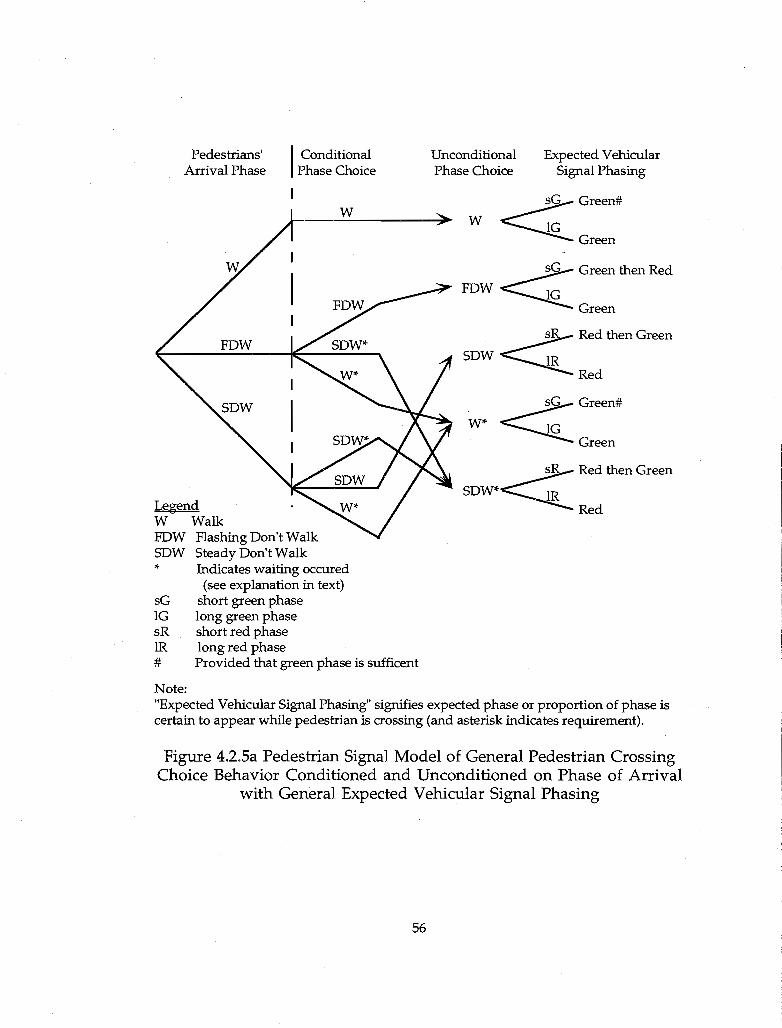
Pedestrians' Arrival Phase I Conditional
Phase Choice
Legend W Walk FDW Flashing Don't Walk SDW Steady Don't Walk
W
,. Indicates waiting occured (see explanation in text)
sG short green phase IG long green phase sR short red phase 1R long red phase # Provided that green phase is sufficent
Note:
Unconditional Phase Choice
Expected Vehicular Signal Phasing
W ~SG Green#
IG Green
~ Green then Red
FDW~ Green
~ Red then Green
SDW~ Red
~Green#
W*~ Green
~ Red then Green
SDW*~ Red
"Expected Vehicular Signal Phasing" signifies expected phase or proportion of phase is certain to appear while pedestrian is crossing (and asterisk indicates requirement).
Figure 4.2.Sa Pedestrian Signal Model of General Pedestrian Crossing Choice Behavior Conditioned and Unconditioned on Phase of Arrival
with General Expected Vehicular Signal Phasing
56

Pedestrians' Arrival Phase
Legend G Green phase R Red phase
I Conditional Phase Choice
I
I G
* Indicates waiting occured sG short green phase lG long green phase sR short red phase lR long red phase
Note:
Unconditional Phase Choice
Expected Vehicular Signal Phasing
~SG Green then Red
G IG Green -
< Red then Green
R lR Red
~SG Green then Red
G* IG Green
< Red then Green
R* lR Red
"Expected Vehicular Signal Phasing" signifies expected phase or proportion of phase is certain to appear while pedestrian is crossing (and asterisk indicates requirement).
Figure 4.2.Sb Vehicular Signal Model of General Pedestrian Crossing Choice Behavior Conditioned and Unconditioned on Phase of Arrival
with General Expected Vehicular Signal Phasing
Each PAR zone will be assessed in terms of hazard indexes and
accident costs. For each intersection, all PAR zones (combined with
hazard indexes, accident costs and compliance rates) will be combined for an overall net safety cost.
If there are more compliant pedestrians when pedestrian signals
and! or crosswalks are present, then the safety differences between different traffic control devices can be quite significant. Next, the
mathematical development of the different types of PARis presented,
starting with the pedestrian aspect.
57

Potential Accident Rate Model - Pedestrian Aspect
The potential accident rates are defined as the possibility that a
vehicle and pedestrian meet in an intersection. To simplify the
concept, PARs are spatially broken down to two levels: 1) the
intersection crosswalks, and 2) its lanes. In additi9n, the PAR is
temporally split into the intersection's signal phases. The pedestrian
aspect of the PAR is composed of its crossing characteristics which is its crossing rate and arrival rate.
The pedestrian lane crossing time is the width of the lane
divided by walk rate. Since pedestrian walk rates are stochastic, they
will have a statistical distribution which is identified and tested in
Chapter 5. Equation 4.2.1 is presented as an example distribution
generator which would create an approximately normal distribution of
walk rates.
WR = x wr + Swr x (RV) Eq. 4.2.1
where WR = walk rate generated from distribution in feet per second
x wr = average walk rate in feet per second Swr = standard deviation of walk rate in feet per second RV = the random variable (from -3.0 to 3.0)
The probability that a pedestrian will have a walk rate and associated crossing timeS, ti, which is equal to w /WR (where w is lane width) is
P(ti). It is assumed that pedestrian walk rates (Le. inverse crossing
times) are independent of signal indications4 (Le. P(tis) = P(ti». Using a
theorem (Meyer, 1970) for transforming continuous random variables,
the distribution for crossing times (assuming that walk rates follow a
3 "i" is used to discretize t because the assumed distribution is not integrable 4 "s" is signal indication
58

normal distribution) is calculated using the average area under the
function's curve as in Equation 4.2.2.
1(1) = [(;i2~)e -(wI'; -~J/2+ (;tl~)e -(W/~l- ~J/2}4-1>1) 12 Eq.4.2.2
where f(t) = probability that pedestrian has walk time, (ti + ti-l)/2 w = lane width in feet t = average crossing time in seconds in (ti - ti-l) increments
where i is increment number of t distribution Jl = mean walk rate in feet per second (j = standard deviation of walk rate in feet per second
The pedestrian arrival time is expected to be independent of the
intersection geometric and traffic characteristics. A representative
statistical distribution for this arrival process is pOisson. However, the
probability that the pedestrian will cross immediately upon arriving at
the intersection is a different problem, dependent on the pedestrian's
crossing behavior as well vehicular characteristics (covered in next section).
Vehicular Component of PAR Zones
The other conflict component is vehicle presence. Without this
component, PARs between vehicles and pedestrians cannot occur. The
vehicle component is affected by six factors: vehicular arrival rate distribution, hourly vehicle volume (for different vehicle
movements), green time for vehicles (and queue dissipation time),
lane widths, stochastic pedestrian walk rates, and number of lanes.
Theoretically, to obtain the vehicular component of PARs, the
expected number of vehicles should be derived from the vehicular
arrival distribution. However, a PAR occurs only when at most one
vehicle hits a pedestrian. Therefore, instead of using the expected
59

number of vehicles arriving, the number of vehicles is derived from
the probability that at least one vehicle arrives (multiplied by one).
Thus the number of vehicles for each potential pedestrian is a fraction
between zero and one.
This vehicular arrival rate distribution can be anyone of many
possible statistical distributions. The poisson distribution, as shown in
Equation 4.2.3, may be appropriate for suburban intersections because
they are commonly isolated, and during many hours have low to
moderate traffic volumes. The probability of one or more vehicles arriving in a lane during time ti is calculated as one minus the
probability of zero arrivals. The number of vehicles present is this
probability multiplied by one.
Eq.4.2.3
where P(Xis 2:: 1) = probability that one or more vehicles arriving in lane Xis = number of vehicles in lane that appears during time ti ti = time in seconds that pedestrian occupies lane Vs = hourly vehicle volume in lane during signal indication
«vehicle volume per hour) X (cycle duration/phase duration)) "3600" = number of seconds per hour
The presence of one or more vehicles depends on the length of time ti
that a pedestrian occupies the lane under consideration. The fraction
of the hour for which the PAR time occurs is largely dependent on the
signal phase timing, but can also be dependent on green time
remaining after vehicular queue dissipation. Pedestrians typically wait
for vehicle queues to dissipate before considering crossing. (In
addition, in multiple lane cases, pedestrians usually wait until all lanes
have completely dissipated queuesi this factor is a function of
intersection congestion.) Calculation of time remaining for pedestrians
to cross the street is directly dependent on the number of vehicles
60

queued during the red phase, hence, dependent on the hourly vehicle
volume, signal phasing, and saturation rate as in Equation 4.2.4 (May,
1988).
where
«C-G)/sat) Tnon-q = C - Tq 1/ sat-V Eq.4.2.4
T non-q = available time for pedestrians to cross (ie. PAR time) in seconds T q = red time plus queue time for vehicles in seconds C = cycle length in seconds G = green time in seconds V = hourly vehicle volume converted into vehicle/second sat = saturation flow rate in vehicles per hour
Combined with the pedestrian component from Section 4.2.2,
the expected number of PARs for a particular crossing time per signal
indication per lane in a crosswalk is shown in Equation 4.2.5
E(PAR/ ti.s.l.c) = [P(xis.? l)][l][P(ti)][Nsc1 Eq.4.2.5
where E(PAR/ti.S.l.C) = expected number of PAR for a particular crossing time per signal indication per crosswalk lane P(Xis 2:: 1) = probability that one or more vehicles arrive in lane 1 = total number of vehicle arriving (multiplied with P(Xis 2:: 1) to obtain expected number of vehicles P(ti) = the probability that pedestrian will cross lane in ti seconds N sc = the total number of pedestrians5 crossing in the crosswalk for the signal phase
Aggregating over all crossing times for all pedestrians, the probability
of a potential accident for a crosswalk lane is shown in Equation 4.2.6.
5 Number of pedestrians is influenced by pedestrian group size which is explained in Chapter 5.
61

n n E(PAR/s.l.c) = L,. [E(PAR/tis·s.l.C)] Ni = L,.[P(XiS? l)][l][P(ti)][Nscl Eq.4.2.6
i=l i=l
where E(PAR/.s.l.c) = expected number of PAR per signal- indication per crosswalk lane N i = total number of pedestrians crossing during signal indication per crosswalk lane n = number of tis slots to be summed
The number of pedestrians crossing a crosswalk during signal indication, Nsc is calculated through multinomial logit analyses which
is presented in the next section. Then, PARs for each lane of each
crosswalk of each signal phase must be calculated before being
multiplied by the representative hazard cost which is described in the
following two sections.
Pedestrian Volume During Signal Phase The number of pedestrians crossing a crosswalk during a signal
indication, Nsc is dependent on the phase and cycle durations,
probabilities of choosing phases, number of lanes and walk rate
distributions. The calculation begins with the probability of pedestrians
arriving during a signal phase which is dependent on the proportion of
pedestrians arriving in that phase (Eq. 4.2.7).
where P[CPa] = probability that pedestrian arrives during phase fs = the proportion of pedestrians arriving in phase 1<1> = phase length c = cycle length
62
Eq.4.2.7

Since the hazard of crossing depends on the actual pedestrian crossing
phase, not the pedestrian arrival phase, the probability of pedestrians
crossing during a particular phase (Eq. 4.2.8) is the summation of all
conditional probabilities as illustrated through Figure 4.2.5.
A P[ cVel = L P[ cVc (l a] Eq.4.2.8
a=l a=l
where P[cVel = probability that pedestrian crosses during phase P[cVc(lal = joint probability that pedestrian is in certain crossing and
arrival phases P[cVc/al = conditional probability that pedestrian crosses during phase given certain arrival phase a = arrival phases up to A arrival phases
Logit analYSis is used to calculate P[cVc/al through segmenting data into
separate analyses based on pedestrian arrival phase as explained in
Section 5.2.
Since the hazard of movement is dependent on whether the
movement occurs during the green or red phase, the probability of
pedestrians crossing for each lane during the signal indication must be
calculated as in Eq. 4.2.9.
ceV ceV P[Gl(lcVvJ = LP[cVGl(lcVd = LP[cVGl/cVel P[cVd Eq.4.2.9
c=l c=l
where P[Gl(lcVvl = probability that pedestrian crosses lane facing green
vehicular signal during particular vehicular signal P[ cVGl (l cVc] = joint probability that pedestrian crosses is in certain green
signal duration and crossing phase P[ cVGl/cVc1 = conditional probability that pedestrian faces green signal
indication during given certain crossing phase c = crossing phase up to C crossing phases in vehicular signal
63

Complex processes are used to calculate P[l\>Gl/l\>cl which depends on
number of lanes, pedestrian arrival times, crossing time distributions,
lane positions, pedestrian and vehicular signal indications, queue
lengths, and start up time. A discretized approach assuming that the
pedestrian arrival rate is evenly distributed in the arrival phase is
currently used in calculating this probability. Results from this
approach are shown in Section 5.2.
Lastly, the number of pedestrians in a crosswalk lane during a
vehicular signal indication is shown in Eq. 4.2.10.
Nsc = P[Gln<l>v1 N/4 Eq.4.2.10
where Nsc = number of pedestrians in crosswalk for signal indication N = total number of pedestrians at intersection "4" is number of crosswalks in intersection
With this number plugged back into Eq. 4.2.6, the number potential
accidents can be calculated. The hazard associated with this potential
accident is broken down into turning movements, which is explained
in the next section.
Hazard Associated with Turning Movements The cost for pedestrians associated with the lane is calculated as a
combination of costs associated with the proportion of left, right, and through vehicular movement encounters as shown in Equation 4.2.11.
64

M
Cis:::: L fmslc * {Om * wlc * CB Eq.4.2.11
m=1
where M is number of movements fmslc is the fraction of turning vehicles per signal indication in lane of
crosswalk rom is the weight assigned to a vehicular turning movement Wlc is lane width in crosswalk CB is the general accident cost per foot of crosswalk per pedestrian (will
be discussed in Section 4.2.4)
Since other research studies have indicated that left and right turns are
more hazardous than through movements, each lane's hazard index is a combination of the hazard (Le. weights, rom) associated with each
movement present in the lane for each approach.
The cost associated with each movement is calculated from
hazard indexes and other accident information presented from three
research studies. First, Knoblauch et al. (1984) characterized pedestrian
hazards based on the exposure measures of 612,395 vehicles and 60,906
pedestrians and associated pedestrian accident data. They calculated
hazard scores by computing ratios of the percentage of pedestrian
accidents to the percentage of vehicle and/or pedestrian population or
vice versa. In keeping the interval scale, they divided the larger
percentage by the smaller percentage. Thus, the hazard scores that are
greater than 1.0 indicate that pedestrians were exposed to more hazards
than normally expected; otherwise these scores are less than -1.0 as
shown in Table 4.2.1.
The signs of the hazard indexes in Table 4.2.1 appear reasonable
except for the diagonal crossing pattern (although little accident data is
known for this maneuver, hence should not be taken for granted). In
addition, the hazard indexes show that the turning maneuvers, except
right-turn-on-red, are not hazardous.
65

Table 4.2.1 Hazard Indexes from Knoblauch et al (1984) Percentage Percentage Hazard
Characteristic Accidents Observed Index
Pedestrian Signal Response: PgdestriiYls With Signal: Green 51.3 90.4 -1.8 Against Signal: Red 46.7 9.6 5.1
Vehicle Action: Vehi!;;ls:s Going Straight 90.0 84.6 1.1 Turning Right 3.8 7.7 -2.0 Turning Left 4.6 7.2 -1.6 Right Tum on Red 1.6 0.5 3.2
Pedestrian Crossing Location: PedestriiYlS Crosswalk 24.0 54.3 -2.3 Within 50' of Intersection 24.1 9.4 2.6 Diagonally Across Inter'n 0.9 1.7 -1.9 Midblock 51.0 34.6 1.5
PV Exposure* Crosswalks:
Not Marked 61.2 24.8 2.5 Marked 38.8 75.2 -5.5
Thus, right-turn-on-green maneuvers are relatively safe. However, it
is unclear what the circumstances are for the left turns (i.e. whether or
not pedestrian movements are allowed during left turn maneuvers).
Hence, another study (Zaidel and Hocherman, 1988) found that most
studies indicate that turning maneuvers are more hazardous. More
specifically, they cited that left turns were noted as three to four times
more hazardous than through movements. The exception to this
trend was their study in Israel which indicated that left turning
maneuvers were safer than through movements only because
pedestrians were not allowed when left turns occurred. Using the data
presented by Zegeer et aI. (1982); the turning maneuvers were
66

recalculated using 15% and 20%6 of movements as left and right turns,
respectively. With this modification, the following hazard indexes
were obtained as shown in Table 4.2.2.
Table 4.2.2 Modified Hazard Indexes Percentage Percentage Hazard
Characteristic Accidents Observed Index
Vehicle Action: Vehicles Going Straight 61.4 65.0 -1.1 Turning Right 14.8 19.5 -1.3 Turning Left w / Peds 22.5 15.0 1.5 Right Turn on Red 1.6 0.5 3.2
For this research, these hazard indexes must be further modified to
allow direct comparisons between different vehicular streams.
Meaning that, all hazard index ratios are created by dividing, the
percentage of the accident population by the exposure population.
Thus, all hazard indexes are positive, and some may be less than 1.0 as
shown in Table 4.2.3.
Hence, the hazard indexes for the turning movements from
Tables 4.2.3 are reflective of the expected turning movement hazard.
Similar modifications to the other hazard indexes in Table 4.2.1 were
made.
Table 4.2.3 Modified Hazard Indexes to be used in Models Percentage Percentage Hazard
Characteristic Accidents Observed Index
Vehicle Action: Vehicles Going Straight 61.4 65.0 0.9 Turning Right 14.8 19.5 0.8 Turning Left w / Peds 22.5 15.0 1.5 Right Turn on Red 1.6 0.5 3.2
6 Zaidel mentioned that turning movements represent 15-25% of all movements.
67

Cost Estimates for Conflicts
To obtain the cost of each pedestrian movement, a general accident cost, CB, per foot of crosswalk is calculated. Three different
sources of information were used for a rough estimate of pedestrian
accident costs as shown in Table 4.2.4. Since all cost estimates are not
current, two inflation factors were applied, one is to reflect the typical
engineering inflation factor - 8%, and the other resembles the medical
costs' inflation factor more accurately - 12%.
Table 4.2.4 General Pedestrian Accident Costs (in Thousands)
Source of Information NHTSA (Biotech) AASmO(R&C) NSC (Zegeer & Deen)
Year 1971 1981 1974
Inflation Rates 12% 8%
$366 $153 $112 $ 67 $ 87 $ 40
Based on pedestrian accident fatality rates of 6.6% in 1971
(Biotechnology, 1973) and 5.9% in 1992 (1992 Traffic Safety Statistics
Report), these estimates were obtained by using a 6% fatality rate. The
National Highway Traffic Safety Administration's estimate was based
on motor vehicle costs, and it appears to be too high. The other sources
of information are more similar and appear to be closer to what is
expected.
The number of accidents expected for a signalized intersection
with less than 1200 pedestrians per day is 0.12 pedestrian accidents per
year (Zegeer, 1982). If we assume that a typical suburban intersection
has two approach lanes in each direction (i.e. four 12-foot lanes plus
two extra feet), the total crosswalk length for a typical intersection is 200
feet (Le. the sum of all four crosswalks). Using The City of Austin's
pedestrian volume base as typical for a suburban-like environment, the
average daily pedestrian volume (conservative estimate) at a typical
intersection is 150. If we use AASHTO's pedestrian accident cost
estimate at a medical inflation rate of 12%, then with all of these factors
68

multiplied, the cost of an accident per person per foot in crosswalk at
an intersection is ($112,000/acc't/year)* (0.12acc't/yr/int) /
(150ped/ day lint * 200ft/int * 365days/yr) = $0.0012 per pedestrian
crossing per foot of crosswalk. However, not all pedestrians cross at
times that are hazardous; in fact, nearly 70% of pedestrians cross when
the light is green. Therefore, the cost of a PAR is 1/(1 - 0.70)($0.0012) =
$0.004 per potential pedestrian accident per foot of crosswalk. For
example, a PAR for one pedestrian for a typical intersection approach (Le. 50 feet wide) costs 20¢: .
E(hazard) = [E(PAR)][ Cls] = C L S n M
= L L L L L [P(xis.? 1)][1] [P(ti)][N][(fmsld(rom)(wld(CB)] c=ll=l s=li=l m=1
Eq.4.2.12 where L is the total number of lanes C is the total number of crosswalks S is the total number of signal indications
Combining Equation 4.2.10 with Equation 4.2.11, the total hazard
cost for the intersection is obtained in Equation 4.2.12.
Summary
With this hazard cost, the delay and equipment cost is integrated
to determine when pedestrian signals are not beneficial. The results of
the testing and integration as well as preliminary examination of the
fundamental questions underlying pedestrian signalization are
addressed in Section 5.4. Next, the model for determining pedestrian
volume input is described.
69

PEDESTRIAN DELAY
Introduction
Like vehicles, pedestrians incur delay at intersections. However,
the delay is not solely caused by signalization only. If all pedestrians
did comply with signalization, then formulating delay would be nearly
straightforward because signalization would be dictated mostly by
vehicular traffic and pedestrian crossing time requirements. In
actuality, some pedestrians comply with signals while other cross
whenever an available gap exists. The framework allows the
estimation of pedestrian delay and assessment of the relative merits of
different pedestrian accommodation strategies.
This framework is developed on the basis of signalization sceme
developed in Section 4.1 and compliance theory developed in Section
4.2.1's Potential Accident Rate Theory. It is adapted here to illustrate
the effects of compliance and signalization.
Pedestrian Delay
Pedestrian delay times for the three possible pedestrian
signalization conditions are examined. Fixed-time pedestrian signals
may force longer cycle lengths to allow pedestrians to cross in
compliance with signals and allow pedestrians experience less delay.
Pedestrian-actuated pedestrian signals may also force longer cycle
lengths when a pedestrian phase is called, but also allow pedestrians to
cross with the green phase. Intersections without pedestrian signals do
not consider pedestrian requirements, and pedestrians may experience
delays and increased non-compliance.
Figure 4.3.1a illustrates pedestrian delay when confronted with
either fixed-time or actuated pedestrian signalization. As no
pedestrians need to wait when facing the steady WALK indication,
there is no delay. Pedestrians arriving during the flashing WALK
indication, have to make choice to whether to wait or cross
70

immediately and some may choose to comply, further increasing their
delay. Pedestrians arriving during the DONT WALK indication
usually have delay especially during the queue dissipation period.
Pedestrians' Arrival Phase
Legend W Walk
Crossing Phase Choice
W
Corresponding Delay
o
o
(G-Wtime)/2 + q + (R-q)/2 = (C-Wtime+q)/2
(G-Wtime)/2 + R
(R-q)/2 + q/2 = R/2
(R-q)/2
FDW Flashing Don't Walk R/2 SDW Steady Don't Walk * Indicates required waiting # Arrival during queue
dissipation period G Green phase length R Red phase length C Cycle length Wtime "Walk" time q queue dissipation time
Figure 4.3.1a Pedestrian Delay Expectation Model due to Vehicular and Pedestrian Signals
71

Figure 4.3.1b illustrates pedestrian delay when confronted with
no pedestrian signalization. As with WALK indication, usually no
pedestrians facing the green need to wait. Pedestrians arriving during
the red phase have to make similar choice decisions as pedestrians
arriving during DONT WALK; they usually have _delay especially
during the queue dissipation period.
Pedestrians' Arrival Phase
Crossing Phase Choice
G
Legend G Green phase R Red phase * Indicates required waiting # Arrival during queue
dissipation period q queue dissipation time
Corresponding Delay
o (R-q)/2 + q/2 = R/2
(R-q)/2
R/2
Figure 4.3.1b Pedestrian Delay Expectation Model due to Vehicular Signals Only
The information for the probabilility that pedestrians will comply or not comply is the same probabilities described in Section 4.2.1. In addition, the probability of arrival is similarly characterized.
Summary
Pedestrian delay formulation is essentially a composite of
vehicular and pedestrian signalization and pedestrian compliance
characteristics. Section 5.2 describes the outcome of the logit
probabilites describing pedestrian compliance, and Section 5.3 describes
72

the outcome of the pedestrian delay models along the vehicular delay
results.
PEDESTRIAN GENERATION RATES
Introduction
With low pedestrian flows, the delay savings benefits of
pedestrian-actuated over fixed-time pedestrian signals are more
apparent. Hence the focus of this effort is to determine when and
where intersections have these relatively low pedestrian generation
rates. Since most pedestrian generation rate studies have been
conducted in downtown or relatively high density areas, those results
are not readily applicable to this study. Hence, the purpose of this
section is to identify mathematical relationships between pedestrian
generation rates and predictor rates for pedestrian signalization
purposes.
This section starts off with theory behind pedestrian generation
rate development. From this, a classification scheme for determining
pedestrian volume is described and illustrated. Finally, a summary is
given in the last section.
Pedestrian Generation Rate Theory
This section presents the theory behind pedestrian generation rates which has two components: 1) the definition development of pedestrian generation rate, and 2) the determination of peak-hour and non-peak hour pedestrian generation rate.
Definition Development of "Pedestrian Generation Rate"
Figure 4.4.1 illustrates the overview of the definition
development of "pedestrian generation rate." The term, pedestrian
generation rate, is not used similarly as in vehicle generation rate
studies where the demand for parking spaces generally depends on the
73

size of the building (e.g. square area, number of chairs). The demand
for the "WALK" indication of pedestrian signals does not depend on
the size of the building as much as it depends on the "mix" and
Group Crossers
I I
---------y---------~ , , I "WALK" Demand Crossers I ~ , ~--------.---------~ I , _______ It ________ ~
I Required "WALK" ~ I I I Demand Crossers I
l(Done in Delay Analyses)l , ~ ,----------------,
Intersection Crossers (Non-rnidblock crossers)
, , .... , r-------~---------, : Legal Definition Concern : I I
-------------------~
Figure 4.4.1 Definition Development of Pedestrian Generation Rate
"distribution" of buildings on opposite sides of streets. At a basic level,
pedestrians who need pedestrian signals are those who cross streets.
This demand is due to the need to get from one site to another site which are separated by street(s). A more appropriate name would be
"pedestrian crossing rate."
It appears that those who need pedestrian signals are those who
cross at the intersection, not those who cross at midblock. It is arguable
to state that those who cross at midblock should not be included in the
pedestrian generation rate. However, pedestrians are obliged to cross at
intersections. Also, many pedestrians who arrive at the intersection
cross at their convenience (by disobeying signals) whenever they can
74

shorten their walking time. Again, one might argue that these
pedestrians do not need pedestrian signals and should not be included
in the pedestrian generation rate. In both types of non-compliance, it is
difficult to prove that all non-compliant pedestrians do not need
. pedestrian signals; hence, at this point, all crossers are jncluded in the
pedestrian generation rate.
Furthermore, if a group of pedestrians arrive and cross at the
intersection together, their crossing time should be no different than a
single pedestrian's crossing time. For example, for a group of three
pedestrians arriving and crossing together, three different crossing
times will not be required, just one. In fact, Palamarthy's behavior
analysis (1993) found that if pedestrian arrivals are in groups, the
behavior among individuals within a group is correlated because of
interactions among them. Hence, each group can be treated similarly as a single demand unit; however, "pedestrian group crossing rate" is
more useful for actuated signal analysis rather than for crossing
analysis.
If pedestrians cross on opposite sides of the road at nearly the
same time, they may also demand the same pedestrian WALK
indication. For example, if a pedestrian chooses path "14" and another chooses "23" at the same time (see Figure 4.4.2), both demands can be
handled in one pedestrian WALK indication. In this respect, "pedestrian group crossing rate" is more accurately named as "pedestrian WALK7 demand rate."
7W ALK and WALK-indication have the same meaning.
75

Comer 1 Comer 4
Comer 2 Comer 3
Note: For this typical intersection, a pedestrian who arrives to comer two and crosses to comer three, his path is labeled as "23."
Figure 4.4.2 Typical Intersection Layout with Labeled Comers
In a more complex scenarior one street may have sufficient green timer but the other street does not. The "pedestrian WALK demand rate"
then becomes the "required pedestrian WALK demand rate." Both
"pedestrian WALK demand rate" and "required pedestrian WALK
demand rate" require the knowledge of cycle length and pedestrian
crossing time to determine when the WALK indication is needed.
Howeverr this approach requires knowing the exact arrival rates of
pedestrians with respect to the variation of signal timing plans.
Insteadr the demand for WALK indications is modeled into the delay
76

framework presented in Section 4.1; hence, the focus is on "pedestrian
crossing rate."s
Pedestrian Generation Rate Analysis: Peak-hour vs. Non-Peak Hour
With the definition of pedestrian generation rates, the next step
is the examination of crossing patterns over time, particularly with
respect to peak hours. At the simplest levet pedestrian volume peak
hour can be defined similarly as vehicular peak-hour. However, this
approach can lead to inaccurate peak-hourdescription(s) of pedestrian
volume. While street network performance is dependent on vehicle
volumes, they are relatively unaffected by pedestrian volumes.
Vehicular traffic is confined to streets because of vehicular dynamics,
and street networks are often operated near capacity during peak-hour.
Pedestrian traffic, on the other hand, have more degrees of freedom in
movement, occupy less space in street networks, and have unlimited
capacity (unless perhaps in downtown areas). Also, vehicle drivers are
affected by latent demand (i.e. the spreading of the peak-hour of
vehicular traffic), but pedestrians are not necessarily affected (unless
they are also vehicle drivers in the same trip). Because of these
differences in vehicular and pedestrian traffic, peak pedestrian
volumes do not need to be defined similarly as the vehicular traffic's
peak hour.
In addition, the time-frame for which peak pedestrian volume
occurs does not need to be restricted to a one-hour period. Peak
volume of pedestrians may occur during a few minutes or several
hours. However, with few sites for peak-period measurements, the
peak-period should not be less than one hour for two reasons: (1)
statistical significance is problematic for short peak periods, and (2) the
other non-peak period(s) of the day would outweigh short peak
SPor the rest of the section, the term "pedestrian generation rate" will be used for simplicity.
77

period(s) in cost/benefit analyses. The time length of each peak period
is determined through regression analyses based on land use and other
factors described in the next section.
When a potential peak-period is detected, its significance must be proven in two tests: (1) the peak-period must have a rate equal to or
higher than a pre-specified reasonable number of pedestrians per hour, and (2) it must be significantly different from the non-peak pedestrian
period(s). A minimum pre-specified number of pedestrians is
necessary to prevent low peak-period volumes from occurring and it is determined by examining actual pedestrian volumes presented in the
next chapter. If a site does not have a peak period, the average rate (over the
data collection time) is used instead. Two regression analyses are
performed using peak and non-peak rates. Where there is no peak or
non-peak rates, average rates were used.
Hence, in this section, the pedestrian generation rate has been
defined as "pedestrian group crossing rate." In addition, peak-hour, non-peak hour, and average pedestrian generation rates were defined. The independent variable for classifying signalized intersections is
presented and illustrated.
Classification Scheme
Previous pedestrian volume studies have used different predictor variables for which those using land use showed the most promise. In practice, generation rates based on land use are commonly used for vehicular trips as in the ITE trip generation rate manual (ITE,
1983). However, very few studies have examined pedestrian
generation rates, especially based on land use in suburban areas. Hence, many different land use variables were examined to
determine how pedestrian generation rate predictor relationships could be developed. Based on these previous studies, a concern for
78

developing pedestrian generation rates based on land use is
transferability. In addition, a larger concern is the methodology
development that would be understandable, quantifiable, and
applicable.
Although the pedestrian generation rate depends on the mix
and distribution of buildings on opposite sides of streets, having an
intensive classification scheme of variables reflecting this distribution
would be far beyond usefulness. In that sense, using land use
surrounding the intersection is perhaps the easiest classification
scheme that is most understandable, quantifiable, and useful.
Therefore, a data collection methodology was designed using a
stratified random sampling technique based on land-use. This
approach serves a dual purpose for the following reason. One objective
of the data collection was to obtain pedestrian generation rate
information, and land-use is a strong explanatory variable. Also, land
use is an exogenous factor to behavior, and it thus would allow
unbiased estimation of safety parameters for Section 5.2. The sampling
strategy also allows for a comparison study by not precluding
intersections from any specific category.
Land-use surrounding a candidate intersection was divided into two concentric zones as shown in Figure 4.4.3. The first zone is defined
by a circle of quarter-mile radius which is the typical pedestrian walking distance. The second zone is a circle of one-mile radius, not including the first zone. It is used to account for inter-zonal trip activity levels.
79

114 mile
Zone 2 1 mile
Figure 4.4.3 Zonal Demarcation of Land Use at the Intersection
As most sites have a mixture of land-use, the dominant pedestrian
generating land-use type was used to classify the intersection. Different
categories were assigned on the basis of quarter- and one- mile characteristics. Five land-use types for the quarter-mile zone and four for the one-mile zone are identified as shown in Table 4.4.1. Though the mixture of land use is important, due to combinatorial effects, a
hierarchical system is used to simplify classification. They are listed in
ascending order of dominance.
Table 4.4.1 Land Use Type for Zones 1 and 2
Ouarter-Mile Zone Residential Minor-Retail Major-Retail Institutional Recreational
80
One-Mile Zone Residential Commercial Institutional Recreational

The above classification gives rise to twenty combinations. The
land-uses are defined as follows. Within the quarter-mile zone,
buildings for residential and other living purposes, and vacant land is
identified under residential land-use. A minor-retail land-use is a
combination of residential land-use with small commercial centers
such as convenience stores and fast-food centers. Major-retail land -use
is identified with shopping malls, major grocery stores, and businesses.
Institutional land-use is comprised of hospitals, schools, universities,
and major multi-floor office buildings where large numbers of
pedestrians are generated. Recreational land-use includes major parks
and recreational centers with large numbers of people accessing them
by foot.
For the one-mile zone, residential land-use is a combination of
both residential and minor-retail land-uses defined earlier. The
commercial land-use is equivalent to the major-retail land-use and the
remaining two land uses have the same definitions as the quarter mile
zone.
As an example application of the classification design, Figure
4.4.4 illustrates a case for which there is minor retail in the quarter
mile zone and commercial land use in the one-mile zone. As shown,
there are other land uses in the zones, but the dominating land use is
the principle criterion for classifying the intersection's land use
variables.
If the intersection under study is in a sparsely populated area, as
in rural areas, the one-mile land-use zone will most likely fall into the
residentialland-use category.
81

One Mile Classification: One-Mile=Cornmercial because of shopping center Quarter-Mile=Minor Retail due to fast food and convenience stores.
Note: Drawing does not represent actual size of buildings. Drawing is exagerated for clarity.
Figure 4.4.4 A Case Study: Minor Retail in the Quarter-Mile Zone and Commercial Land Use in the One-Mile Zone
Summary Expected pedestrian volume patterns at signalized intersections
was described for both peak and non-peak periods. In addition, useful
predictor variables based on land use was briefly described and
illustrated.
SUMMARY
From this theoretical framework, the pedestrian generation rate,
pedestrian delay and safety and vehicular delay concepts were
presented. The results and implications from the data collection and
further analyses are presented in the next chapter.
82

CHAPTER 5. MODELING RESULTS
INTRODUCTION
Using the models developed in Chapter 4, data were obtained to
determine the results of the pedestrian generation rate and compliance
characteristics as well as the overall results of pedestrian signalization.
PEDESTRIAN GENERATION RATE
Introduction The 20 land-use combination methodology presented in Section
4.3 to the City of Austin was applied to initially test the procedure'S
robustness as well as the city's land use proportion. After the data was
collected, statistically analyses were conducted to determine the final
robustness of the procedure for which minor adjustment were made
and regression analyses were done.
Application of Data Collection Methodology In order to test the robustness of the procedure, the methodology
was applied to intersections in the Gty of Austin, Texas. The city has
approximately 500 traffic-signalized intersections, of which about 200 were selected from all geographical regions (e.g. northwest Austin).
They were classified based on a priori knowledge, with the aid of a
map, and in some cases, a visit to the intersection. On a map of Austin, most of the major commercial centers, institutions, and recreational facilities are clearly marked and could be identified with ease. The
distribution of the intersections from this design procedure is shown in
Table 5.1.1. For purposes of the survey, a site from each subset was
randomly selected. Since the object of this data collection was also to
obtain information on the distribution of pedestrian crossings over
time, each site was surveyed for a duration of five to six hours.
83

Table 5.1.1 Distribution Of Intersections By Land Use
LAND-USE INTERSECTIONS
1 mile zone 1/4 mile zone # (%) Residential 10 (5.21)
Residential Minor retail 18 (9.38)
[55] Major retail 10 (5.21)
(28.65%) Institutional 16 (8.33)
Recreational 1 (0.52)
Residential 10 (5.21)
Commercial Minor retail 17 (8.85)
[57] Major retail 23 (11.98)
(29.69%) Institu tional 4 (2.08)
Recreational 3 (1.56)
Residential 12 (6.25)
Institutional Minor retail 19 (9.90)
[57] Major retail 7 (3.65)
(29.69%) Institutional 15 (7.81)
Recreational 4 (2.08)
Residential 7 (3.65) Recreational Minor retail 4 (2.08)
[23] Major retail 2 (1.04)
(11.98%) Institutional 1 (0.52)
Recreational 9 (4.69)
A video recording technique was used to obtain information on
pedestrian behavior. The advantage of using video is that information
could be reviewed repeatedly, thus assuring higher data credibility.
The video with time recorder was setup at one intersection comer and
was operated only when a pedestrian was crossing.
Pedestrian events (e.g. walking times) were measured using a
continuous time-event recorder. With this instrument, time intervals
between events could be measured to an accuracy of 0.1 second. The
84

time intervals are recorded similarly in the manner that stopwatches record events except that it stores up to 30 time intervals.
The task of decoding information from the video tapes was
shared by two scorers. In order to ensure consistent interpretation of
variable definitions, an inter-scorer reliability check was also
performed. The flow-chart in Figure 5.1.1 illustrates the procedure.
Process Video Data by Scorer 1
Select 30 observations from an intersesction
Process Video Data by Scorer 2
'----illl'l Compare outputs of 1 & 2 ~----'
Observe Video together and refine variable definitions
Select 30 observations randomly
Figure 5.1.1 Inter-Scorer Data Reliability Procedure
85

Preliminary Statistics
As described in Section 4.3.2, the methodology for choosing sites
included a two-tier classification. The dominant land use in the 1-mile
radius included residential, commercial, institutional, and recreational
areas. The dominant land use in the quarter-mile .radius included residential, minor-retail, major-retail, institutional, and recreational
areas.
The pedestrian generation rate derived is not simply pedestrian
volume over time. As explained in the last section, if arrivals are in
groups, the behavior among individuals within a group is correlated
because of interactions among them. However, the behavior across
groups can still be assumed independent when the group arrivals are
independent. Consequently, the pedestrian generation rate is taken as
the number of groups (including one-person groups) over time.
From the data collected, the average lS-minute pedestrian count
for the quarter-mile land use is presented in Figure 5.1.2. As shown,
the residential and minor retail land uses generate similar levels of
pedestrians while major retail and recreational land uses are similar.
Institutional land use appears to generate more than twice as many
pedestrians as any other category. The average lS-minute pedestrian count for the 1-mile land use
is presented in Figure 5.1.3. As shown, the residential land use appears to generate a very small number of pedestrian trips. In contrast, the three other land uses generate three to four times more.
Figure 5.1.4 shows the results of all land uses combined over the period during which the data was collected; the average 1S-minute
pedestrian volume shows considerable variation over the period of the
day. In order to determine when peak and non-peak times occur,
hourly volumes were calculated using these lS-minute counts at each
lS-minute interval (Figure 5.1.5). It appears that there are three peak
times starting: (1) shortly after 8 am, (2) at the end of the lunch hour - 1
86

pm, and (3) shortly before 4 pm. These patterns seem to replicate
known travel activity as morning peak hour, lunch hour, and evening
peak hour.
The hourly distribution (calculated similarly as in Figure 5.1.5)
for each land use (within the quarter-mile) period is shown in Figure
5.1.6. The most evident feature is the high volume of pedestrians
generated from the institutional land use, which also shows a
prominent lunch hour. It also appears to peak in the evening, but this
peak is not as high as the morning. Although its morning peak hour
appears visible, its peak is not much higher than the other morning
hour volumes. Perhaps more surprising is that the other land uses
generate similar pedestrian volumes in the morning hours, but in the
afternoon, the major retail and recreational land uses appear to
increase substantially. The minor retail land use is rather constant
during the day.
The hourly distribution for each land use (in a one-mile radius)
over the time period for the one-mile land use is shown in Figure 5.1.7.
In this case; the residential land use exhibits a consistently low
pedestrian volume at all times. The recreational land use has a high
pedestrian volume in the peak hour including the highest morning
peak hour. The commercial land use has the highest peak lunch hour
whereas the afternoon peak hour is mixed between the commercial and institutional land use.
The results from the quarter and one-mile land uses were
heavily influenced by sites that have high pedestrian volumes. For
instance, the site with the highest pedestrian generator in the one-mile
recreational land use had an institutional land use in the quarter-mile
radius; based on visual inspection at the site, it appears that this
quarter-mile land use appeared to have more influence than its one
mile land use.
87

These results point out the need to re-examine land use as a
predictor variable and explore other variables that will
variation within the land use categories. In the next
collection for this exploration is described.
explain the
section, data
12
CI)
S 10
::s -10
" " " " " " " " " " " " " " " " " " " " a
> 8 t:: cO ..... .... ....
" " " " " " " " " " " " " " " " " " " " " " " " " " " " " " " " " " " " " " " " " " " " " CI) 6 Q)
"0 - " " " " " " " " " " " " " " " " " " " " Q)
0... Q) 4 co cO .... Q) ::- 2 <
0
" " " " " 3.8 " " " " " 3.6 " " " " " " " " " " " " " " " " " " " " " " " " " 2.3 " " " " " " " " " " " " " " " 2.1 " " " " " " " " " " " " " " " " " " " " " " " " " " " " " " " " " " " " " " " " " " " " " - " " " " " " " " " " " " " " " " " " " " r " "" ":) " " " " " " " " " " " " " " " " " " " " ... ... ... ... ... " " " " " " " " " " " " " " " " " " " " '" -' -' -' -' " " " " " " " " " " " " " " " " " " " " ... ... ... ... ... " " " " " " " " " " " " " " " " " " " " -' -' -' '" -' " " " " " -' -' '" '" '" " " " " " " " " " " " " ... ... ... ... ... " " " " " i' " " " " " " " " " " " " " -' '" rl' '" ", " " " " " ,/' ./' '" .I' ,If " " " " " " " " " " Residential Minor Retail Major Retail Institutional Recreational
Quarter-Mile Land Use
Figure 5.1.2 Average is-Minute Pedestrian Volumes by Quarter-Mile Land Use
8
CI) Q) 6.3 S
.E 6
~ a
5.8 " " " " " " " " " " " " " " " " " " " " " " " " " " " " " " " " " " " " " " " " " 4.7 " " " " " " " " " " " " " " " " " " " " " " " " " " " " " " " " " " " " " " " " " " " " " " " " " ..... .... ..... 4 CI)
Q)
" " " " " " " " " " " " " " " " " " " " " " " " " " " " " " " " " " " " . " " " " " " " " " " " " " " " " " " " " " " " " " " " " " " " " " " " " " " " " " " " " " " " " " " " " " " "0 Q)
0... Q)
co cO 2 .... Q)
::-<
" " " " " " " " " " " " " " " " " " " " " " " " " " " " " " " " " " " " " " " " " " " " " " " " " " " " " " " " " " " " " " " " " " " " " " " " " " " " " " " " " " " " " " " " " " " " " " " " " " " " " " " " " " " " " " " " " " " " " " " " " " " " " " " " " " " " " " " " " " " " " " " " 1.5 " " " " " " " " " " " " " " " " " " " " " " " " .- " " " " " " " " " " " " " " " " " " " " " " " " " " " " " " " " " " " " " " " " " " " " " " " .-" " " " " " " " " " " " " " " " " " " " " " " " " " " " " " " " " " " " " " " " " " " " " " " " " " " " " " " " " " " " " " " " " " " " " " " " " " " " " .- " .- " " " " " " " " .-
" " " " " " " " " " " " " " " " " " " " " " " " .- " " " " " " " " " " " " " .- " " " " " " " " '" " " " " " " " " " " " " " " " " " " " " " " " " 0 " " " " " " " " " " " " " " " " " " " " " " " " Residential Commercial Institutional Recreational
One-Mile Land Use
Figure 5.1.3 Average is-Minute Pedestrian Volume by One-Mile Land Use
88

26 (].I 24 S :l 22 .-0
>-:: 20 til 18 :8 ell
16 (].I
"'C:i (].I
0.., 14 (].I .... 12 :l .S
10 :::E , 11')
8 ,.., (].I OJ:) 6 til 10< (].I 4 > <:
2
0 7 9 11 13 15 17
24-hr Time of Day
Figure 5.1.4 Average IS-Minute Pedestrian Volume over all Land Use
26 24
S 22 :l - 20 0 >-g 18
..... 16 10<
ti (].I
14 "'C:i (].I
0.., 12 >. "i: 10 g ::r:: 8
(].I
co 6 til 10<
~ 4 <£:
2 0
7 9 11 13 15 17
24-hr Time of Day
Figure 5.1.5 Average Hourly Pedestrian Volume over all Land Use
89
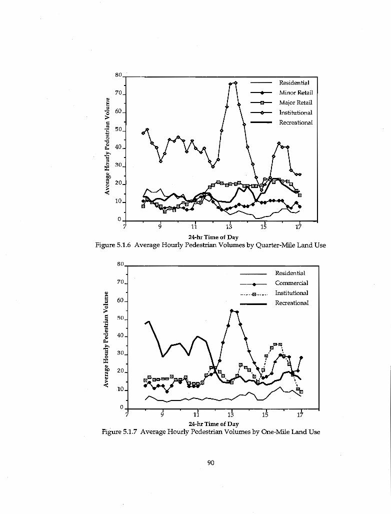
80
70 Col E :;$
60 -0
> I:C
'" 50 '1:: -Q) Col 'tI
~ 40 ;:....
'i: :;$ 0 30 ::c Q,I bI)
G 20 ~
-< 10
0 7 9 11 13
24-hr Time of Day
Residential
• Minor Retail
--m-- Major Retail
• Institutional
Recreational
15 17
Figure 5.1.6 Average Hourly Pedestrian Volumes by Quarter-Mile Land Use
80
70
Q,I
E 60 :;$ -0
> I:C 50 <'is
:s '" Q,I 'tI 40 ~ ;:.... '§ 30 0 ::c Q,I bI) 20 e Q,I
~ 10
0 7 9 11 13
240hr Time of Day
• _._--13-._.,
15
Residential
Commercial
Institutional
Recreational
17
Figure 5.1.7 Average Hourly Pedestrian Volumes by One-Mile Land Use
90

Results of Pedestrian Generation Rate Regression Analyses
Thus through numerous regression analyses, it was found that
land use is the strongest indicator of pedestrian volumes. Hence, the
analysis on pedestrian volume predictor variables is focused on the
quarter-mile and one-mile land use variables.
The order of the quarter-mile land uses by increasing mean
pedestrian generation rate is listed as the following:
1 - Residential 2 - Minor Retail 3 - Recreational 4 - Major Retail 5 - Institutional
However, there is considerable variability that cannot be
explained by one dominant quarter-mile land-use characteristics.
Unexplained variability in the pedestrian generation rate for the
quarter-mile radius is due to two factors. First, the presence of a major
parking lot/garage across a street from a major land use (i.e. major
retail, institutional) forces people to cross the street. Second, the
presence of a retail establishment across a street from a land use with
many people that have little auto access, particularly high school
students at lunch hour, causes many people to cross the street. These
two factors are similar to reasons of high pedestrian generation rates in downtown areas; therefore, these two sites were excluded from further analyses to prevent their influence from distorting regression analyses
on low pedestrian volumes.
Based upon experience with variability in the quarter-mile land
use, experimentation was performed on the one-mile land use deleting
the sites with major parking and school-commercial activity
interactions. Since these variables are significant, they tended to
interact with the one-mile land use effect. Without these sites, the
91

modified one-mile land use form is in the following order of
increasing mean generation rate:
1 - Residential 2 - Commercial (including recreational) 3 - Institutional
This approach allowed the basic variability to be explained more
accurately by the one-mile land use which improved the ability of the
model to explain the variability in the generation rate, though the very
small number of these types of sites in our' sample does not allow high
R-squares.
The method of determining the pedestrian generation rates
based on land use is the separation of peak hour(s) from the non-peak
hours. Table 5.1.2 shows specifications for the prediction of peak hour
and non-peak hour volumes. The models apply to intersections
without major parking and without school/ commercial interaction;
hence, low pedestrian volumes can be predicted with these models.
Table 5.1.2: Models For Pedestrian Generation Rates
Variable Name
Constant 1/4-Mile Res.& Minor Retail LU One-Mile Res. Land Use One-Mile Institutional Land Us
Number of Observations Significance of F-statistic Adjusted R-Squared
Peak Model (ped/hour)
coefficient (t-stat) 19.26 (7.45)
-10.38 (-3.97) - 8.40 (-2.53) 11.82 (3.87)
18 .000 .760
Non-Peak Model (ped/hour)
coefficient (t-stat) 6.30* (3.89)
11.22 (4.31)_
18 .001 .508
.. Note: if the one-mile land use is residential and the quarter-mile land use is residential or minor retail, then the non-peak hour generation rate is 0.6.
From the peak and non-peak hour generation rate regression models,
the reuslting 15 land-use combination is illustrated in Table 5.1.3.
These rates and times are used in the analyses in Section 5.3.
92

Table 5.1.3 Pedestrian Generation Rate for Land Use Combinations
One Mile Land Quarter-Mile Peak Peak Non-Peak Non-Peak Use Land Use PGR Hours PGR Hours
Residential Residential - - 0.60 7am-llpm
Residential Minor Retail - - 0.60 7am-llpm
Residential Recreational 10.86 4pm-5pm 6.30 7am-4pm, 5pm-11pm
Residential Major Retail 10.86 12pm-4pm 6.30 7am-12pm, 4pm-llpm
Residential Institutional 10.86 4pm-5pm 6.30 7am-4pm, 5pm-llpm
Commercial/ Residential 8.88 8am-12pm 6.30 7am-8am, Recreational 12pm-llpm
Commercial! Minor Retail - - 6.30 7am-llpm Recreational
Commercial/ Recreational 19.26 4pm-5pm 6.30 7am-4pm, Recreational 5pm-llpm
Commercial! Major Retail 19.26 12pm-4pm 6.30 7am-12pm, Recreational 4pm-11pm
Commercial! Institutional 19.26 4pm-5pm 6.30 7am-4pm, Recreational 5pm-llpm
Insti tu tional Residential 20.70 Bam-12pm 17.52 7am-8am, 12pm-11pm
Institutional Minor Retail - - 17.52 7am-llpm
Institutional Recreational 31.08 4pm-5pm 17.52 7am-4pm, 5pm-11pm
Institutional Major Retail 31.08 12pm-4pm 17.52 7am-12pm, 4pm-11pm
Institutional Institutional 31.08 4pm-5pm 17.52 7am-4pm, 5pm-11pm
93

· SAFETY AND BEHAVIOR ANALYSES
Behavior Analysis
A descriptive analysis was conducted to study the basic
compliance characteristics of pedestrians for intersections with and
without pedestrian signals. This approach illustrates when
signalization benefits occur.
Data from different intersections are pooled depending on the
presence or absence of a pedestrian signal as well as which phase
pedestrians arrived on as explained in Section 4.2.2. A total of 712 and
231 intersection crossings were observed at signalized and unsignalized
intersections, respectively. The number of arrivals and crossings on
each signal indication are reported in Table 5.2.1. The percentage of
pedestrians making an illegal crossing (i.e. crossing on Steady Don't
Walk (SDW) or RED) is less at signalized compared to unsignalized
intersections. Also, most pedestrians arriving on a Flashing Don't
Walk (FDW) cross immediately, and only a small fraction wait for
WALK indication. Table 5.2.1 Arrivals And Crossings At Signalized And
Unsignalized Intersections Signalized Intersections
Crossing on Arrival on Walk Flashing OW Steady OW Total
Walk 88 (96) 3 (3) 1 (1) 92 Flashing OW 7 (9) 59 (74) 14 (17) 80 Steady OW 327 (61) 23 (4) 190 (35) 540
Total 422 85 205 712
Unsignalized Intersections Crossing on
Arrival on Green Red Total Green 78 (96) 3 (4)
I 81
Red 77 (51) 73 (49) 150 Total 155 76 231
Numbers in brackets denote percentages; the sum may be different from 100 due to rounding.
94
Results of Logit Modeling of Compliance Rates
The understanding of pedestrian compliance as outlined in
Chapter 4 begins with multinomial logit analyses of pedestrian
response to signalization. As explained, pedestrian compliance is
dependent on when pedestrians arrive at the signalized intersection.
Thus, the data is segmented into five sets for which three are analyzed
for compliance characteristics: pedestrians arriving on Steady Don't
Walk (SDW), on Flashing Don't Walk (FDW) and on Red where no
pedestrian signal exists. The two data sets for which pedestrians arrive
on WALK or on Green where no pedestrian signal exists do not need
to be analyzed since virtually all those pedestrians cross during that
phase. Based on the numbers of available data points, results for
pedestrians arriving on steady don't walk or during the red phase
when there is no pedestrian signal, was expected to be promising.
However, because of insufficient data points, results for pedestrians
arriving on flashing don't walk are less promising, but still worth
examining.
The type of variables used in the logit modeling analyses are
associated with intersection characteristics: total number of lanes and
crossing width, number of approach lanes and its crossing width, speed,
type of median, and vehicular volumes. In addition, many dummy variables, composite variables and different levels of details were
analyzed, representing over 200 different variations examined. Logit
analysis was performed for each of the three different scenarios: Pedestrians arriving on "Steady Don't Walk," "Flashing Don't Walk"
and on "Red Phase" (Le. no pedestrian signal). Some information
presented in the section on Pedestrians Arriving on Steady Don't Walk
is the same as for the other sections (e.g. correlation analyses).
95
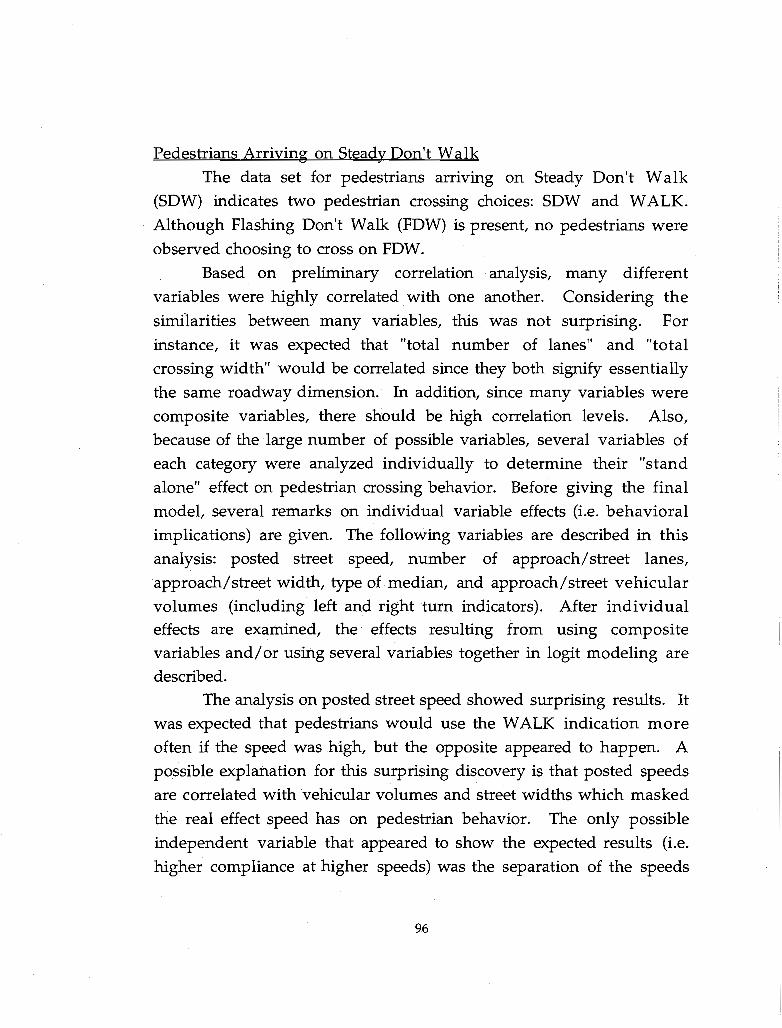
Pedestrians Arriving on Steady Don't Walk
The data set for pedestrians arriving on Steady Don't Walk
(SDW) indicates two pedestrian crossing choices: SDW and WALK.
Although Flashing Don't Walk (FDW) is present, no pedestrians were
observed choosing to cross on FDW.
Based on preliminary correlation analysis, many different
variables were highly correlated with one another. Considering the
similarities between many variables, this was not surpnsmg. For
instance, it was expected that "total number of lanes" and "total
crossing width" would be correlated since they both signify essentially
the same roadway dimension. In addition, since many variables were
composite variables, there should be high correlation levels. Also,
because of the large number of possible variables, several variables of
each category were analyzed individually to determine their "stand
alone" effect on pedestrian crossing behavior. Before giving the final
model, several remarks on individual variable effects (i.e. behavioral
implications) are given. The following variables are described in this
analysis: posted street speed, number of approach/street lanes,
approach/street width, type of median, and approach/street vehicular
volumes (including left and right tum indicators). After individual effects are examined, the effects resulting from using composite
variables and/ or using several variables together in logit modeling are
described.
The analysis on posted street speed showed surprising results. It
was expected that pedestrians would use the WALK indication more
often if the speed was high, but the opposite appeared to happen. A
possible explanation for this surprising discovery is that posted speeds
are correlated with vehicular volumes and street widths which masked
the real effect speed has on pedestrian behavior. The only possible
independent variable that appeared to show the expected results (i.e.
higher compliance at higher speeds) was the separation of the speeds
96

into 30 and 35+ mph categories; however, this method just hides the
contradictory effect. In other words, using this variable type hid the
non-linear effect of speed on pedestrian compliance. Separating the
other variables' effects on speed is needed, but not likely to be possible
because real world conditions do not allow all combinations of speed
and vehicular volume / street width to occur. For example, many
residential streets are two-lane roads with low volumes and speed
limits; very few would have high speeds nor high volumes.
The analysis on the number of approach lanes appeared to
follow expectations. Though there were some discrepancies, it was
found that the higher the number of lanes the more likely pedestrians
would be using the WALK indication. Using a dummy variable
separating the number of approach lanes from 1-3 lanes from 4+ lanes
appeared promising. Using the total number of lanes produced similar
results, perhaps even more promising. Separating the total number of
lanes into 2-4, 5-6, and 7+ lanes also appeared promising.
The analysis on the approach width also produced consistent
results. If a dummy variable separating total width into <40 feet and
40+ feet was used, the results are the same as the dummy variable for
the number of approach lanes because of the 100% correlation between
the two variables or otherwise said, all streets with 4+ lanes have a
width of 40+ feet. Using a dummy variable separating the total width
into 0-40,40-100, and 100+ feet appeared promising.
Also initially promising are two types of median. First, raised concrete medians that are most typically typecast as medians was
almost significant, and it appeared that pedestrians were more likely
NOT to cross during the WALK signal because of it. Second, two-way left turn lanes (TWLTL) produced the opposite effect. Perhaps,
pedestrians felt they could not predict when vehicles would turn into
these dual usage lanes; hence, they were less apt to cross than when
these TWLTL are absent.
97
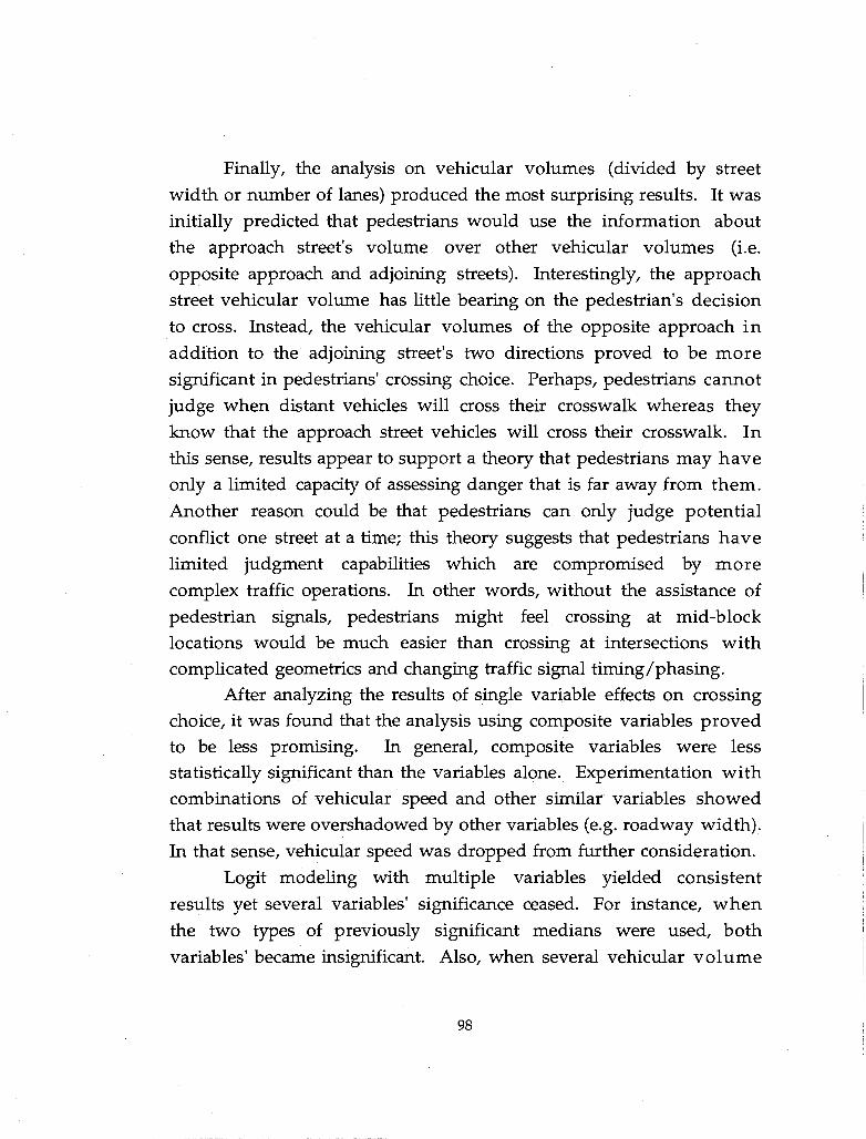
Finally, the analysis on vehicular volumes (divided by street
width or number of lanes) produced the most surprising results. It was
initially predicted that pedestrians would use the information about
the approach street's volume over other vehicular volumes (i.e.
opposite approach and adjoining streets). Interestingly, the approach
street vehicular volume has little bearing on the pedestrian's decision
to cross. Instead, the vehicular volumes of the opposite approach in
addition to the adjoining street's two directions proved to be more
significant in pedestrians' crossing choice. Perhaps, pedestrians cannot
judge when distant vehicles will cross their crosswalk whereas they
know that the approach street vehicles will cross their crosswalk. In
this sense, results appear to support a theory that pedestrians may have
only a limited capacity of assessing danger that is far away from them.
Another reason could be that pedestrians can only judge potential
conflict one street at a time; this theory suggests that pedestrians have
limited judgment capabilities which are compromised by more
complex traffic operations. In other words, without the assistance of
pedestrian signals, pedestrians might feel crossing at mid-block locations would be much easier than crossing at intersections with
complicated geometrics and changing traffic signal timing/phasing. After analyzing the results of single variable effects on crossing
choice, it was found that the analysis using composite variables proved to be less promising. In general, composite variables were less statistically significant than the variables alone. Experimentation with
combinations of vehicular speed and other similar variables showed
that results were overshadowed by other variables (e.g. roadway width).
In that sense, vehicular speed was dropped from further consideration.
Logit modeling with multiple variables yielded consistent
results yet several variables' significance ceased. For instance, when
the two types of previously significant medians were used, both
variables' became insignificant. Also, when several vehicular volume
98

variables were used together, the approach street volume still
remained insignificant.
More importantly, when the different vehicular volume rate
variables were used together, very different coefficient estimates and
insignificances occurred. For instance, when the side street volume
variables were used together, the variable for the side street
representing left turning vehicles ceased to be significant, and both
variables had diminished coefficient values. The most likely reason
for this is that vehicular volume rates for both adjoining street
approaches are correlated; hence, a volume rate variable representing
both adjoining street volumes at once proved to be more reliable.
However, using the opposite street volume with the adjoining
approach street volume caused the opposite street volume to be
insignificant.
When determining which model would become final, all
previous significance issues were taken into consideration. Also, the
fact that several variables were highly correlated to one another limited
the scope of possible models. A few models came up with all variables
being correct, consistent, and significant; out of these, one was chosen
based on its applicability to the desired modeling efforts. Table 5.2.2
shows the model for pedestrians arriving on Steady Don't Walk and
choosing to wait for WALK:
Table 5.2.2 Logit Model for Pedestrians Arriving on Steady Don't Walk and Choosing Walk over Steady Don't Walk
Variable Value Constant -1.74 Alane 0.289 Svolan 0.00368
Note: Alane = Number of Approach Lanes Svolan = Side Street Vehide Volume per Lane
99
t-stat. -3.62 3.19 3.70

Pedestrians Arriving on Flashing Don't Walk
Unlike the data set for pedestrians arriving on Steady Don't
Walk (SDW), the data set for pedestrians arriving on Flashing Don't
Walk (FDW) did not have the benefit of substantial data size with
significant information for each phase choice. In addition, the FDW
data set has three different choices: pedestrians choosing to cross on
existing FDW, waiting and then crossing on SDW, or choosing to wait
for crossing on WALK. This extra choice requires that the FDW data
set be larger than the SDW data set.
Even with these disadvantages, the FDW data set was analyzed
for any possible pedestrian compliance characterization. As expected,
the results from the multinomial logit analysis did prove to be very
limited and contradictory. Significant and possibly significant cases are
reported.
With respect to adjoining street vehicular volume rate variables,
pedestrians were more likely to cross on FDW (and to lesser degree on
WALK) as volumes increased. This was probably the most consistently
expected result because increased hazard usually prompts compliance.
Pedestrians were also more likely to cross during FDW when a
grass median was present. In other words, when given a wide rather
natural median, pedestrians were more likely to attempt crossing
because of the safety net of having a median to buffer them against
possible phase changes.
Pedestrians were less likely to cross during the FDW when speed
is higher. A possible explanation for this is that pedestrians, not
knowing when the signal would change, opted to wait, even at the
chance of crossing against the signal (during SDW).
Perhaps the most surprising result was that when there was 5+
lanes (or greater width), pedestrians were less likely to cross during the
100

WALK or FDW phase. This effect is probably the result of some other underlying unexplained effect due to lack of sufficient data size.
The overall characteristic from this FDW analysis that seems to
appear is that the FDW phase seems to encourage non-comformant
behavior. Because of the compliance characterizations problems, the
market share was used as the FDW model because of the lack of data set
size which could mislead research results.
Pedestrians Arriving on Red Phase (no pedestrian signal present)
As explained before, the data set for pedestrians arriving on the
red phase is sufficient in size and phase proportion. Like the data set
for pedestrians arriving on Steady Don't Walk, this data set has only
two choices, but only because just two choices are available: crossing on
Red or Green.
However, the multinomial logit analysis showed very little
predictive results. This output probably signifies that pedestrians do
not depend on traffic and geometric conditions to determine in the
absense of pedestrian signals whether or not to comply with vehicular
signals. None-the-Iess, significant and possibly significant cases are
reported. Pedestrians appeared to be more likely to choose the green phase
when the vehicular volume rate is higher. Though this trend is
similar as in the other data sets, the significance is much less prominent.
Pedestrians also appeared to cross during the green phase when speed was 35+ mph. However, when examining speed on a full scale, this dummy variable masked the contradictory effect as explained in
the section on pedestrians arriving on SDW.
One surprising result is that in the absence of pedestrian signals,
pedestrians were more likely to cross during the green phase when
101

crosswalks were provided. However, when testing this effect for when
pedestrian signals were provided, there was no significance.
As with the FDW data set, the market share was used to
represent the results from this data set.
Modeling Inputs
Values used for the variable inputs for the developed integrated
model need to mirror realistic suburban environments. Using the
twenty intersections from Section 5.1, information was obtained from
the City of Austin regarding vehicular volumes. Typical suburban
vehicular volumes range from 100 to 400 vehicles per lane per hour.
Results from this vehicular volume level indicate that for fixed
timed vehicular signals without pedestrian signalization, the cycle
lengths tended to be less than 30 seconds with exception of
intersections with 400 vehicles per lane per hour for both major and
minor streets. Since municipalities generally do not allow cycle
lengths to be less than 30 seconds, the minimum cycle lengths were set
to 30 seconds and the green light split to critical flows.
For fixed-timed vehicular signals with pedestrian signals, cycle
lengths tended to be 30 seconds or greater, up to 135 seconds. When the critical volume for both streets were equal, cycle lengths were identical
regardless of vehicle volume level. Likewise, when similar splits in green phases were used, cycle lengths were similar regardless of vehicle volume levels.
Using typical suburban values as vehicular volumes between
100 to 400 vehicles per lane and one to three lanes per approach, logit
results differed significantly as shovvn in Table 5.2.3. As expected, as the
number of vehicles on the side street increased and/or as the number
of approach lanes on the crossing street increased, pedestrians generally
tended to comply with pedestrian signals.
102

Table 5.2.3 Example Logit Model Results for Pedestrians Arriving on Steady Don't Walk and Choosing Walk over Steady Don't Walk
Number of Approach Lanes 1 3
Side Street 100 0.25 0.38 Vehicle Volume 200 0.33 0.47
per Lane 400 0.51 0.65
Next, results from the safety model using these compliance rate
are illustrated.
Potential Accident Rate (PAR) Trends
Pedestrian crossing safety was mathematically modeled using
the Potential Accident Rate (PAR) methodology as described in Section
4.2. The components include the hazard rates and accident costs as well
as the walk rate, number of lanes, compliance rates, vehicular and
pedestrian volumes, signal timings, and other variables. The
complexity of this method is briefly shown in the appendix as a sample
outcome of one scenario (i.e. base case). Many other steps which were
described in Section 4.2 are not shown, but none-the-Iess important.
The safety model outcomes are described in terms of costs for easier
understanding of results and implications. The safety cost is described through different geometric and traffic conditions: pedestrian volume,
vehicular volume, number of lanes, and signal type. In addition,
specifications for the inputs following typical suburban characteristics are described above.
The base case as shown in the appendix consists of the following
characteristics in Table 5.2.4. It is the basic two-phase fixed-time signal
with pedestrian signals for which each street has 4 lanes (Le. 2 approach
lanes) and 200 vehicles per lane. In addition, its 19.26 pedestrians per
103

hour represent the pedestrian peak hour for several land use
combinations (as shown in Table 5.1.3).
Table 5.2.4: Base Case Specifications Component number of phases pedestrian volume pedestrian signal? fixed/ actuated timing? major street:
number of lanes vehicular vol/lane
minor street: number of lanes vehicular vol/lane
Specification 2
19.26 yes
fixed
4 200
4 200
This base case output shows a hazard cost of $0.57. In other
words, for the entire intersection with the specifications just described,
the expected hazard cost amounts to a rather small amount.
This hazard cost varied linearly with pedestrian volume by design. In other words, through randomization and walking rate
variation, the mathematical process behind hazard cost was found not
to be influenced by pedestrian volume. Thus obtaining the hazard cost
only required the rate to be directly multiplied by pedestrian volume.
This effect is possible only if two conditions hold: crossing group size typically consists of one pedestrian and pedestrian volume is low (Le.
likelihood of more than one pedestrian in signal cycle is small). Since suburban pedestrian volumes and group sizes are very low, these
assumptions are possible. None-the-Iess, the range of hazard costs for
suburban areas range from the nearly non-existent $0.02 (for 0.6
pedestrians per hour) to some level more significant $0.92 per hour (for
31.1 pedestrians per hour).
The hazard cost increases non-linearly when vehicular volume
increases. At very low volumes (Le. less than 200 vehicles per lane per
104

hour), the relationship is primarily linear because higher probability of
vehicles not platooning. However, at higher volumes, the hazard rate
starts to level off because once vehicular platoons become a regular
feature of congested roadways, the chances of pedestrians interacting
with each vehicle is much smaller. The expected hazard costs due to 50
to 400 vehicles per lane per hour ranges from $0.16 to $0.96 per hour.
The hazard cost also increased at a decreasing rate when the
number of lanes increased. Though it might be expected that changes
in the number of lanes would produce greater changes in hazard cost
than vehicular volume changes, lane functions also depend on
vehicular patterns. The changes ranged from $0.30 to $0.78 for
configurations ranging from 2X2 to 6X6 lanes for each street.
All in all, hazard cost is small. Comparing different signal types
showed the smallest change. Many times signalization benefits do not exceed $0.10. The reason behind this very small change is that the
hazard cost method dimishes the role compliance plays in pedestrian
safety. Though compliance differences could be significantly different,
not all compliant scenarios are safe for some types of movements. As
mentioned in Section 5.2.1, many pedestrians arriving on Flashing
Don't Walk, cross immediately whether or not the green phase is
ending and face an impending red light. Without pedestrian signals,
there is also the danger of facing the red when crossing near the end of
the green phase. In the next section, the safety cost is compared to other model
components, and the role of suburban land use in pedestrian
signalization is explained.
SCENARIO ANALYSIS FOR SUBURBAN AREAS
The approach taken to study the combinatorial effect of all four
factors, namely pedestrian and vehicular delay, safety, and equipment
costs, was the base case scenario re-examination. Next, an analysis with
105

respect to pedestrian/vehicular volume patterns (i.e. peak/non-peak
hours from Section 5.1.3) and fixed/actuated signals is given.
The base case scenario produced the following costs as in Table
5.3.1. The most noticeable effect is that vehicular delay is
approximately 100 times larger than the hazard cost. The magnitude of
pedestrian delay is also small and as mentioned in Section 4.1.2,
pedestrian delay changes are small. Upon pedestrian signal installation, pedestrian delay increases because compliance increases
and in some cases, signal timing increases. The equipment cost is a
constant in all pedestrian signal installation cases.
Table 5.3.1: Base Case Costs Component lHazard (PAR) ~edestrian Delay iVehicular Delay !Equipment*
Cost 0.57 1.05 65.33 0.32
*Note: Additional cost due to pedestrian signalization installation
The trends of pedestrian signalization benefits associated with
these four factors are discussed with respect to fixed and actuated Signalization types.
Fixed Pedestrian/Vehicular Cycle Times
The benefit outcome regarding fixed pedestrian cycles compared
to fixed vehicular cycles is categorized by whether or not the pedestrian
cycle is longer than the vehicular cycle.
If the vehicular cycle is shorter than the pedestrian cycle, then
with the pedestrian traffic requirement causing higher vehicular
delays, fixed pedestrian cycles are costly. This scenario is likely to occur
during non-peak times when optimal vehicular cycles are shorter than
pedestrian cycles.
106

If the vehicular cycle is longer than the pedestrian cycle, then
pedestrian signalization does not impact vehicular delay. The
comparison is then between pedestrian delay, hazard and equipment
cost. However, the differences of pedestrian delay and equipment costs
can offset the gain by pedestrian hazard costs. This scenario is likely to
occur during peak times when high vehicle volumes cause longer cycle
lengths.
However, daily traffic demands have peak and non-peak hours.
With the fixed pedestrian/vehicular signal scenario, non-peak hour
costs dominate the possible benefit fixed pedestrian signals may have
during peak hour times.
These results seem contradictory to the idea of installing
pedestrian signals in the first place. In theory, pedestrian signals'
primary function is to increase pedestrian phases where needed when
vehicular traffic signals do not meet crossing time needs. However, as
explained, suburban fixed pedestrian signals point to large vehicular
delay costs. Hence, potential benefit with fixed pedestrian cycles can
only be realized when pedestrian signal timing does not require longer
than optimal vehicular signal timing.
Actuated Pedestrian/Vehicular Cycle Times
As with fixed pedestrian timing, actuated pedestrian timing is discussed with respect to cycle timing.
If the vehicular cycle is shorter than the pedestrian cycle, then
pedestrian requirements cause vehicular delay which is proportional to
the number of cycles used by pedestrians. As explained in Section 4.1.2,
this relationship is not linear with the number of pedestrians; in other
words, once all cycles are occupied by pedestrians, then it doesn't
matter how many more pedestrians arrive to cross. Hence, in this case,
the smaller the number of pedestrians at an intersection, the less
vehicular delay is experienced. Also, additional pedestrian delay is
107
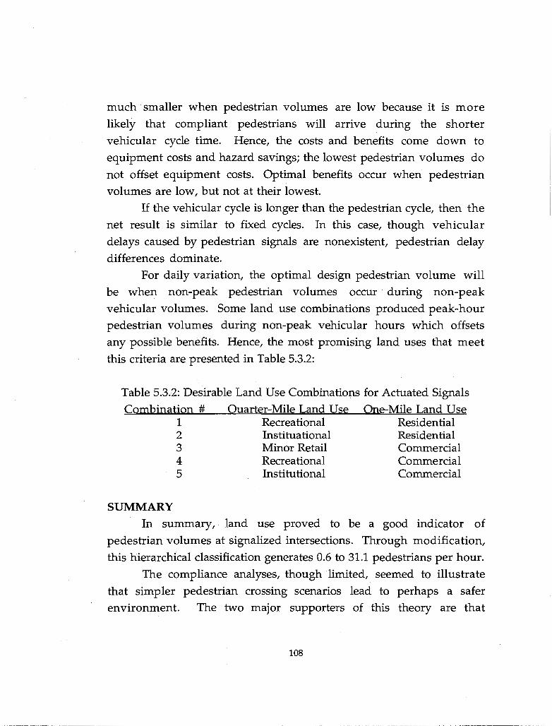
much smaller when pedestrian volumes are low because it is more
likely that compliant pedestrians will arrive during the shorter
vehicular cycle time. Hence, the costs and benefits come down to
equipment costs and hazard savings; the lowest pedestrian volumes do
not offset equipment costs. Optimal benefits occur when pedestrian
volumes are low, but not at their lowest.
If the vehicular cycle is longer than the pedestrian cycle, then the
net result is similar to fixed cycles. In this case, though vehicular
delays caused by pedestrian signals are nonexistent, pedestrian delay
differences dominate.
For daily variation, the optimal design pedestrian volume will
be when non-peak pedestrian volumes occur during non-peak
vehicular volumes. Some land use combinations produced peak-hour pedestrian volumes during non-peak vehicular hours which offsets
any possible benefits. Hence, the most promising land uses that meet
this criteria are presented in Table 5.3.2:
Table 5.3.2: Desirable Land Use Combinations for Actuated Signals
Combination # Quarter-Mile Land Use One-Mile Land Use 1 Recreational Residential 2 Instituational Residential 3 Minor Retail Commercial 4 Recreational Commercial 5 Institutional Commercial
SUMMARY
In summary, land use proved to be a good indicator of
pedestrian volumes at signalized intersections. Through modification,
this hierarchical classification generates 0.6 to 31.1 pedestrians per hour.
The compliance analyses, though limited, seemed to illustrate
that simpler pedestrian crossing scenarios lead to perhaps a safer
environment. The two major supporters of this theory are that
108
......................................... -~--- ----------_ ... --_ ..

compliance rates increase when the number of lanes increase and/or
side street volume increases. Also, pedestrians will cross when given
the opportunity especially when medians are provided.
The safety analyses, PAR rates, on the other hand show very
little benefit associated with compliance. In all, pedestrian hazard costs·
is relatively small compared to vehicular delay costs. This effect
heavily affected the possible pedestrian signalization outcomes
especially with fixed pedestrian signalization. For different land uses, the effect of pedestrian signalization over
time varies significantly since vehicular/pedestrian peak/non-peak
hours may not coincide. Possible land use patterns for warranting
actuated pedestrian signals were suggested.
109

110

CHAPTER 6. CONCLUSIONS AND RECOMMENDATIONS
The objective of this study has been to develop an integrated
approach to assess delay, safety, and behavior (i.e. compliance) in a
single framework for a suburban signalized intersection. In order to
accomplish this objective, the study was divided into four objectives.
First, delay models were developed to incorporate pedestrian behavior
to determine pedestrian impact on vehicle and pedestrian signals.
Second, mathematical functions for pedestrian compliance and
behavior were developed to evaluate pedestrian safety. Third, land use
patterns were studied to determine impact on suburban pedestrian
volume patterns. Fourth, different traffic control strategies were tested
to determine suburban environment impact on vehicle and pedestrian
signalization. The findings of these four objectives are summarized as
the following conclusions and recommendations:
(1) The delay model allowed practical examination of vehicular and pedestrian delay. Extending Webster and Newells' equations for
fixed and actuated timing, respectively, is very useful for determining
pedestrian impact. Incorporation of pedestrian behavior allowed
reduction of expected pedestrian delay and actual pedestrian signal
response timing.
(2) Pedestrian behavior was mathematically modeled as a
balance between the two extreme pedestrian safety indicators: conflict (underestimate) and exposure (overestimate). This method, the
potential accident rate (PAR), allows the safety indicator to be
scientifically based rather than a statistical estimate which could change
over time. PAR is an estimation based on physical proximity, phasing,
and volume levels rather which is significantly less than the
multiplication of sheer pedestrian and vehicle volumes as in the
exposure measure. On the other hand, PAR is a method that allows
111
every close encounter between pedestrian and vehicular to be
characterized as an encounter whereas the traditional conflict method
requires that an observer determine whether or not pedestrians and/or
vehicles reacted toward one another in the roadway.
(3) Pedestrian compliance, using multinomial logit, in a
suburban setting was found to have several unique characteristics. The foremost findings are that pedestrians are more compliant on wider
streets and higher volumes on adjoining streets. Medians seem to
encourage non-compliant behavior (except for the two way left turn
lanes). 'Compliance with respect to speed had very mixed results. The
overall evidence shows that pedestrian signals show some promise in
increasing pedestrian compliance given certain traffic/ geometric
situations.
(4) General results from the integrated model showed that
vehicular delay would dominate the outcomes. Though safety benefits
occurred with different signalization strategies, the amount was small
as with pedestrian delay and equipment costs. This effect caused fixed
timing schemes to be costly when pedestrian timing requirements were
greater than optimal vehicular signal cycle timings.
(5) Land use variables appear to be useful in characterizing pedestrian generation (i.e. crossing) rates. The useful quarter-mile
categories are residential, minor and major retail, recreational and institutional land uses. The useful one-mile categories are residential, commercial, and institutional land uses. The overall pedestrian
generation rates ranged from a low of 0.6 to a high of 31.1 pedestrians
per hour which is significantly lower than the range of suburban
vehicular volume rates. These categories also have distinct peak/non
peak volume patterns.
(6) The peak/non-peak hour volume patterns affected the
outcomes of the integrated model. During low vehicular volume
periods (i.e. vehicular non-peak periods), low pedestrian volumes
112

should predominate. During peak vehicular periods, high pedestrian
volumes should predominate. Thus, pedestrian peak and non-peak
periods should coincide with vehicular volume patterns as welL
Examining these characteristics, promising land uses following this
pattern include those with quarter-mile zones of recreational and
institutional land uses for all one-mile land uses, particularly
residential and commercial land uses.
Recommendations
The following recommendations are based upon the modeling
efforts, analysis, and conclusions. They are intended to point out
needed future research as well as point out other types of closely related
research ideas.
(1) The transferability of the behavioral and generation rate
results to other suburban areas should be studied to determine regional
differences. Since Austin, Texas has year-round warm weather, a
primary concern is the effect of cold weather upon pedestrian traffic
characteristics. In addition, a useful and insightful approach to
understanding the pedestrian phenomena is to study the effect of
different cultures by comparing pedestrianism between different
countries.
(2) An interesting issue is the effect transit systems have 0 n
pedestrian volume patterns. First, the Austin transit system currently
consists of buses, and like most U.S. suburbs, relies heavily on
automobiles for typical passenger traveL Cities with more extensively
developed transit systems may have significantly different pedestrian
travel patterns. Second, the Austin school students are usually
transported by bus; hence, the effect of students on the traffic system is
smaller. Other cities not having a school bus system will likely
experience different pedestrian volumes. Third, the Austin transit
113

system has a policy of providing bus stops at relatively fixed distances
apart whether or not they are needed; this phenomena made the
possible independent variables relating to transit difficult to use. In the
absence of this policy, it would be interesting to determine the true
effect transit has on pedestrian volume patterns.
(3) Though these models were used for the pedestrian crossing phenomena, further studies could be performed to determine
effectiveness for other engineering applications. For instance,
pedestrian generation rates might be studied for sidewalk volumes.
These analyses, results and conclusions should encourage other
researchers to study suburban environments separately as a unique
entity not only for the pedestrian phenomena, but also for other
transporta tion systems.
114

APPENDIX
115

116
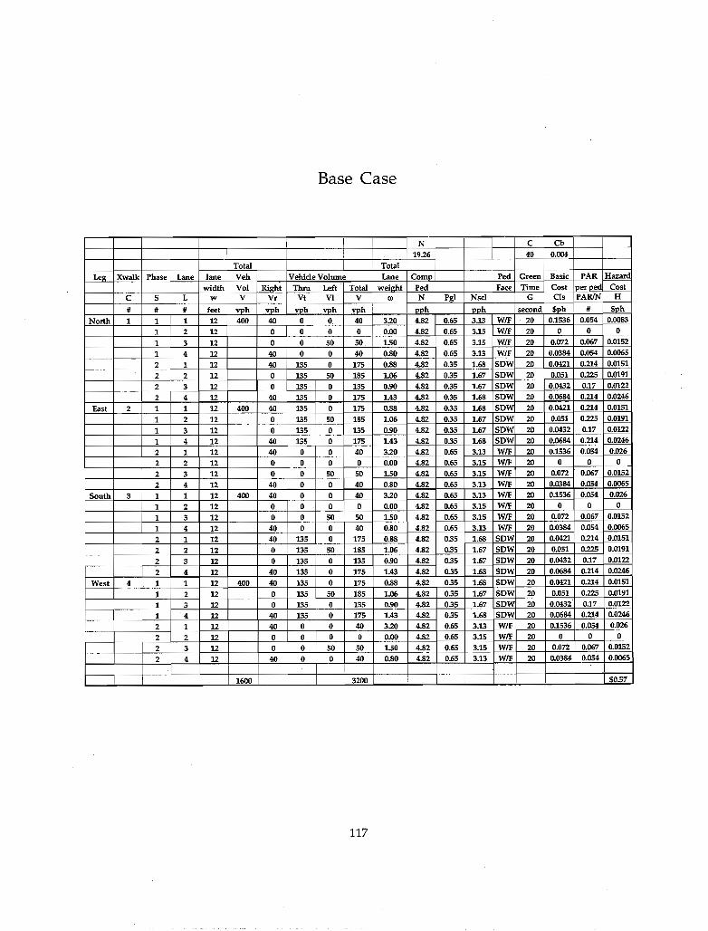
Base Case
N Cb
Phase Lane
S L w
# #
North 1 1 1
1 2 12 0 0 1 :3 12 0 0 1 4 12 40 0 2 1 12 40 135 2 2 12 0 135 2 3 12 135 2 4 12 40 135 0
East 2 1 1 12 400 40 135 0 1 0 135 50 1 0 135 0
135 0 0
40 0 0 0 0
40 0 40 0 0
12 West 12 400
12 3 12 0.0122
1 4 12 0.0246
2 1 12 40 0.054 0.026
2 2 12 0 4.82 0 0
2 3 12 0 1.50 4.S~ .. 0.067 0.0152
:2 4 12 40 O.SO 4.82 WIF 20 0.054 0.0065
1600 SO.57
117

118

REFERENCES
Abrams, C. and Smith, S. "Selection of Pedestrian Signal Phasing/' Transportation Research Record #629, JHK & Associates, 1977a, pp. 1-6.
Abrams, C. and Smith, S. "Urban Intersection Improvements for Pedestrian Safety. Volume III Signal Timing for the Pedestrian," BioTechnology, Inc., 1977b.
Adams, W. "Road Traffic Considered as Random Series," Journal of the Institute of Civil Engineering #4,1939, pp. 121-130.
Bailey S., Jones, S., Stout, R., Bailey, J., Kass, S. and Morgan B. "Issues of Elderly Pedestrians/' Transportation Research Board paper #984, 1991.
Behnam, J., and Patel, B. itA Method for Estimating Pedestrian Volume in a Central Business District/, Transportation Research Record # 629, 1977, pp. 22-26.
Braun, R., and Roddin, M. "Quantifying the Benefits of Separating Pedestrians and Vehicles, "NCHRP Report #189, Transportation Research Board, 1978.
Cynecki, M. "Development of a Conflicts Analysis Technique for Pedestrian Crossings," Transportation Research Record #743, 1980, pp. 12-20.
Daganzo, C. "Estimation of Gap Acceptance Parameters Within and Across the Population from Direct Roadside Observation/' Transportation Research, Vol. 15B, 1981, pp. 1-15.
Davis, S., King, L. and Robertson, H. "Predicting Pedestrian Crosswalk Volumes," Transportation Research Record #1168,1988, pp. 25-30.
Davis, S. Robertson, H., and King, E. "Pedestrian /Vehicle Conflicts: An Accident Prediction Model," Transportation Research Record #1210, 1989, pp. 1-11.
119

Fleig, P., and Duffy, D. "A Study of Pedestrian Safety Behavior Using Activity Sampling," Traffic Safety, Dec 1967.
Garder, P. "Pedestrian Safety at Traffic Signals: A Study Carried out with the Help of a Traffic Conflict Technique," Accident Analysis & Prevention. Vol 21 #5, 1982, pp. 435-444.
Griffiths, J., Hunt, J., and Marlow, M. "Delays at Pedestrian Crossings: 1) Site Observations and The Interpretation of Data," Traffic Engineering & Control, July/August 1984a, pp. 365-371.
Griffiths, }., Hunt, J., and Marlow, M. "Delays at Pedestrian Crossings: 2) The Development and Validation of a Simulation Model of a Zebra Crossing," Traffic Engineering & Control, October 1984b, pp. 505-509.
Griffiths, J., Hunt, J., and Marlow, M. "Delays at Pedestrian Crossings: 3) The Development and Validation of a Simulation Model of a Pelican Crossing," Traffic Engineering & Control, December 1984c, pp. 611-616.
Griffiths, J., Hunt, J., and Marlow, M. "Delays at Pedestrian Crossings: 4) Mathematical Models," Traffic Engineering & Control, May 1985, pp. 277-282.
Hill, M. "Walking Straight Home from School: Pedestrian Route Choice by Young Children," Transportation Research Record #959, 1984, pp. 51-55.
Hocherman, I., Hakkert, A. and Bar-Ziv, J. "Estimating the Daily Volume of Crossing Pedestrians from Short-Counts," Transportation Research Record #1168. 1988, pp. 31-38.
Hoel, L. "Pedestrian Travel Rates in Central Business Districts," Traffic Engineering, Jan. 1968, pp. 10-13.
Khasnabis S., Zegeer C., and Cynecki, M. "Effects of Pedestrian Signals on Safety, Operations, and Pedestrian Behavior - Literature Review," Transportation Research Record #847, 1982, pp. 78 - 86.
120

King, G. "Pedestrian Delay and Pedestrian Signal Warrants," Transportation Research Record #629, KLD Associates Inc., 1977, pp. 7-13.
Knoblauch, R., Tobey, H., and Shunaman, E. "Pedestrian Characteristics and Exposure Measures," Transportation Research Record #959, 1984, pp.35-41.
Mahmassani, H., and Sheffi, Y. "Using Gap Sequences to Estimate Gap Acceptance Functions," Transportation Research, Vol. 15B, 1981, pp. 143-148.
Miller, A. "Nine Estimated Gap Acceptance Parameters," Traffic Flow & Transportation (g.f. by Newell Ed.), New York: Elsevier, 1972, pp. 215-236.
Morrall, J., Ratnayake, L. and Seneviratne, P. "Comparison of Central Business District Pedestrian Characteristics in Canada and Sri Lanka," Transportation Research Record #1294, 1991, pp. 57-61.
Mortimer, R. "Behavioral Evaluation of Pedestrian Signals," Traffic Engineering, Nov. 1973, pp. 22-26.
Newell, G. "Theory of Highway Traffic Signals," Institute of Transportation Studies - University of California @ Berkeley, 1989.
Palamarthy, S., Mahmassani, H., and Machemehl, R. "Characteristics of Pedestrian Crossing behavior at Signalized Intersections," Technical Report 1296-1, Center for Transportation Research, The University of Texas at Austin, 1993.
Pushkarev, B. and Zupan, J. "Pedestrian Travel Demand," Highway Research Record #355, 1971, pp. 1-15.
Reiss, M. "Knowledge and Perceptions of Young Pedestrians," Transportation Research Record #629, BioTechnology Inc., 1977, pp. 13-18.
121

Robertson, H. and Carter, E. "Criteria/Warrants for Pedestrian Signal Indications," Institute of Transportation Engineers, Washington D. c., 1984a.
Robertson, H. and Carter, E. "The Safety, Operational, and Cost Impacts of Pedestrian Indications at Signalized Intersections," Transportation Research Record #959, 1984b, pp. 1-7.
Rouphail, N. "Midblock Crosswalks: A User Compliance and Preference Study," Transportation Research Record #959, 1984, pp. 41-47.
Sandrock, K. "Heuristic Estimation of Pedestrian Traffic Volumes," Transportation Research, Vol22A #2,1988, pp. 89-95.
Seneviratne, P. and Javid, M. "Estimating and Updating Flows on Pedestrian Facilities in the Central Business District," Transportation Research Record #1281, 1990a, pp. 97-101.
Seneviratne, P. and Morrall, J. "Estimation of Flow for Evaluating and Classifying Pedestrian Facilities," Journal of Advanced Transportation, Vol. #1, 1990b, pp. 31-46.
Smith, S. et aL "Planning and Implementing Pedestrian Facilities in Urban and Developing Rural Areas," Research Report, NCHRP 294A, 1987.
Tanaboriboon, Y. and Guyano, J. "Analysis of Pedestrian Movements in Bangkok," Transportation Research Record #1294, 1991, pp. 52-56.
Texas Manual on Uniform Traffic Control Devices [TMUTCD] , Section 4,1980.
Virkler, M. "Pedestrian Flows at Signalized Intersections," Transportation Research Record #847 I 1982, pp.72-77.
Witkowski, J. "Accident Type Designations and Land Use Data in Pedestrian Accident AnalysiS," Transportation Research Record #1168, 1988, pp. 45-48.
122

Zaidel, D. and Hocherman 1. "Safety of pedestrian Crossings at Signalized Intersections," Transportation Research Record #1141, 1988, pp.1-6.
Zegeer, C. and Deen, R. "Pedestrian Accidents in Kentucky," Transportation Research Record #629, 1977, pp. 26-28.
Zegeer, c., Khasnabis, S. and Fegan, J. "Development of Improved Pedestrian Warrant for Traffic Signals," Transportation Research Record #904, 1983, pp. 58-67.
Zegeer, C., Opiela, K., and Cynecki, M. "Effect of Pedestrian Signals and Signal Timing on Pedestrian Accidents," Transportation Research Record #847,1982, pp. 62-71.
123