an analysis of basic investment strategies: buy-and-hold
TRANSCRIPT

University of Central Florida University of Central Florida
STARS STARS
Retrospective Theses and Dissertations
Summer 1982
An Analysis of Basic Investment Strategies: Buy-And-Hold and An Analysis of Basic Investment Strategies: Buy-And-Hold and
Market Timing Market Timing
David L. Hansen University of Central Florida
Part of the Business Commons
Find similar works at: https://stars.library.ucf.edu/rtd
University of Central Florida Libraries http://library.ucf.edu
This Masters Thesis (Open Access) is brought to you for free and open access by STARS. It has been accepted for
inclusion in Retrospective Theses and Dissertations by an authorized administrator of STARS. For more information,
please contact [email protected].
STARS Citation STARS Citation Hansen, David L., "An Analysis of Basic Investment Strategies: Buy-And-Hold and Market Timing" (1982). Retrospective Theses and Dissertations. 630. https://stars.library.ucf.edu/rtd/630

AN ANALYSIS OF BASIC INVESTMENT STRATEGIES: BUY-AND-HOLD AND MARKET TIMING
BY
DAVID LUDWIG HANSEN B.A., Yale University, 1961
MB.A., Harvard University, 1966
THESIS
Subffiitted in partial fulfillment of the requirements for the Master of Arts degree in Applied Economics
in the Graduate Studies Program of the College of Business Administration
University of Central Florida Orlando, Florida
Summer Term 1982

TABLE OF CONTENTS
Chapter I. DEVELOPMENT OF THE STUDY . . . . . 1
II. METHODOLOGY . . . . . . . . . . . . • • 12
III. FINDINGS • • • . . • 16
IV. CONCLUSIONS . . .. . • 37
SELECTED BIBLIOGRAPHY • 39

LIST OF TABLES
1. Results of a Buy-and-Hold Strategy, Initial Investment of $10,000 . . . . . . . . . . . 18
2. Results of Market Timing Strategy #1, Initial Investment of $10,000, Base Period • . . . . . 19
3. Results of Market Timing Strategy #1, Initial Investment of $10,000, Test Period . . . . . . 20
4. Results of Market Timing Strategy #2, Initial Investment of $10,000 ••••.•.•.•..• 21
5. Results of a Buy-and-Hold Strategy, Monthly Investment of $100 • • • . • . • • . . • . 22
6. Results of Market Timing Strategy #1, Monthly Investment of $100, Base Period •••••• 23
7. Results of Market Timing Strategy #1, Monthly Investment of $100, Test Period •••.•••. 24
-
8. Results of Market Timing Strategy #2, Monthly Investment of $100 • . . . . . . • .
9. Analysis of Market Timing Strategy #l . 10. Analysis of Market Timing Strategy #2 • . . 11. Results of Combined Buy-and-Hold and Market
Timing Strategy #1, Initial Investment of
. 25
. 27
. . . 28
$10,000 •••••••••••••••.•••. 30
12. Results of Combined Buy-and-Hold and Market Timing Strategy #1, Monthly Investment of $100 • • • • • • • • • • • • • • • • • • . • • 31
13. Results of Combined Buy-and-Hold and Market Timing Strategy #2, Initial Investment of $10,000 •••••••••••••••••••• 33
14. Results of Combined Buy-and-Hold and Market Timing Strategy #2, Monthly Investment of $100 • • • • • • • • • • • • • • • • • • • 34
15. Analysis of Risk and Return •••••• • • • 36

CHAPTER I
DEVELOPMENT OF THE STUDY
There are probably as many investment strategies as
there are investors. The one thread common to most of them
is that they do not work. Numerous studies have shown that,
on average, professional investment managers cannot out
perform the market (Rolo 1982). When fees are taken into
consideration, these professionals underperform the market.
The results of the majority of professional
investment managers are part of the public record and lend
themselves to objective analysis. No such accumulation of
data is available to measure the success or failure of the
amateur investor. Yet, few have even advanced the theory
that the amateur can do as well as the professional.
The random walk hypothesis provides a partial
explantion of the above observations. It holds that
movements of stock prices are not predictable, as they are
independent of previous changes. These early studies tend
to destroy the technical theory approach, as it is based
on the exact opposite hypothesis - that stock and
commodity prices are predictable on the basis of past
experience.

2
The narrow form of the random walk hypothesis has
been stated as follows (Malkiel 1973):
The history of stock-price movements contains no useful information that will enable an investor consistently to outperform a buy-and-hold strategy in managing a portfolio.
The broad form of the random walk hypothesis has
been summarized by Professor Samuelson (Malkiel 1973):
If intelligent people are constantly shopping around for good value, selling those stocks they think will turn out to be overvalued and buying those they expect are now undervalued, the result of this action by intelligent investors will be to have existing stock prices already have discounted in them an allowance for their future prospects. Hence, to the passive investor, who does not himself search out for under- and overvalued situations, there will be presented a pattern of stock prices that makes one stock about as good or bad a buy as another. To that passive investor, chance alone would be as good a method of selection as anything else.
-The broad form of the random walk hypothesis is
similiar to the efficient capital market theory.
Efficient capital market theory builds on the random walk
hypothesis and labels all security analysis as useless in
predicting future stock prices. It maintains that all
information is known to the investing public so that
existing prices relect everything that is predictable or
anticipated. If the market has already discounted the
future, there is not much room for even the superior
analyst to beat the market. Thus, fundamental analysis
is no more helpful than technical analysis in an
investment strategy.
3
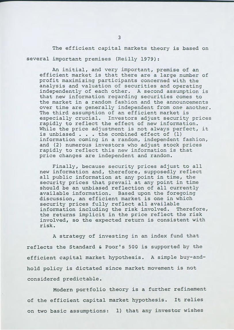
The efficient capital markets theory is based on
several important premises (Reilly 1979):
An initial, and very important, premise of an efficient market is that there are a large number of profit maximizing participants concerned with . the analysis and valuation of securities and operating independently of each other. A second assumption is that new information regarding securities comes to the market in a random fashion and the announcements over time are generally independent from one another. The third assumption of an efficient market is especially crucial. Investors adjust security prices rapidly to reflect the effect of new information. While the price adjustment is not always perfect, it is unbiased • • • the combined effect of (1) information coming in a random, independent fashion, and (2) numerous investors who adjust stock prices rapidly to reflect this new information is that price changes are independent and random.
Finally, because security prices adjust to all new information and, therefore, supposedly reflect all public information at any point in time, the security prices that prevail at any point in time should be an unbiased reflection of all currently available information. Based upon the foregoing discussion, an efficient market is one in which security prices fully reflect all available information including the risk involved. Therefore, the returns implicit in the price reflect the risk involved, so the expected return is consistent with risk.
A strategy of investing in an index fund that
reflects the Standard & Poor's 500 is supported by the
efficient capital market hypothesis. A simple buy-and-
hold policy is dictated since market movement is not
considered predictable.
Modern portfolio theory is a further refinement
of the efficient capital market hypothesis. It relies
on two basic assumptions: 1) that any investor wishes

4
to maximize the returns from his investment; and 2) that
investors are basically risk averse, which means simply
that, given a choice between two assets with equal rates
of return, an investor will select the asset with the
lower level of risk (Reilly 1979).
The portfolio model requires i .nvestors to
quantify their risk variable. The purpose of the model
is to derive the expected rate of return and an expected
risk measure for a portfolio. The variance of the rate
of return is a meaningful measure of risk. The variance
or standard deviation of expected returns is a statistical
measure of the dispersion of .returns around the expected
value. The greater the dispersion, the gr~ater the degree
of uncertainty surrounding future r~turns (Markowitz 1952).
Markowitz showed the importance of diversification
for reducing risk by relating expected return for an
individual asset to expected return for a portfolio of
assets. He went on to develop the efficient frontier
concept which relates risk to return for a number of
alternative portfolios. Those portfolios that show the
gr~atest return for each alternative level of risk appear
on the efficient frontier. The investor can select the
optimum portfolio consistent with his individual risk
preference.
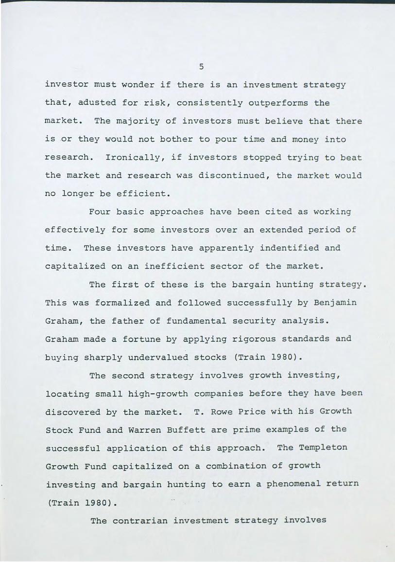
Given the efficient market hypothesis, the
5
investor must wonder if there is an investment strategy
that, adusted for . risk, consistently outperforms the
market. The majority of investors must believe that there
is .or they would not bother to pour time and money into
research. Ironically, if investors stopped trying to beat
the market and research was discontinued, the market would
no longer be efficient.
Four basic approaches have been cited as working
effectively for some investors over an extended period of
time. These investors have apparently indentified and
capitalized on an inefficient sector of the market.
The first of these is the bargain hunting strategy.
This was formalized and followed successfully by Benjamin
Graham, the father of fundamental security analysis.
Graham made a fortune by applying rigorous standards and
buying sharply undervalued stocks (Train 1980).
The second strategy involves growth investing,
locating small high-growth companies before they have been
discovered by the market. T. Rowe Price with his Growth
Stock Fund and Warren Buffett are prime examples of the
successful application of this approach. The Templeton
Growth Fund capitalized on a combination of growth
investing and bargain hunting to earn a phenomenal return
(Train 1980).
The contrarian investment strategy involves

6
bargain hunting of a sort. Its main advocate, David
Dreman .(.1979), achieved notable success through the
purchase .of out-of-favor stocks with very low price/
earnings ratios. His work shows that the stocks with
the lowes~ P/E ratios consistently outperform the stocks
with the highest P/E ratios.
These first three investment strategies involve
the selection of individual stocks and their application
requires extensive research on the part of the investor
or his advisor. The successful practitioners tend to
have fairly large staffs to conduct their research. This
is obviously not practical for the average investor.
The market timing approach is the forth basic
strategy. This approach does not depend on the selection
of individual stocks as do the three other strategies.
One can invest in an index fund and follow this game plan.
It is possible and probably advisable to pursue this
strategy while following any of the other three. If a
stock represents a bargain at the market peak, it must b e
an even better bargain at the market trough - all other
things being equal. The investor would stand to benefit
from the recovery of the market in addition to market
recognition of the individual stock.
A definitive study of market timing was performed
by William F. Sharpe (1975). He points out that:

7
The investment manager who hopes to outperform his competitors . usually expects to do so either by the selection of securities within a given class or by the allocation of assets to specific classes of securities. Potentially, one of the most productive forms of the latter strategy is to hold common. stocks during bull markets and cash equivalents during bear markets (market timing) •
In a perfectly efficient market, any attempt to obtain performance superior to that of the overall "market portfolio" (taking into account both risk and return) by picking and choosing among securities would fail. Although few investment managers are ready to admit that U. S. security markets are completely efficient, there is a growing awareness that inefficiencies are .few: any divergence between the price of a security and the "intrinsic value" that would be assigned to it by well informed and highly skilled analysts is likely to be small, temporary and difficult to identify in advance. Empirical studies of the performance of professionally managed . portfolios yield results consistent with this view: few, if any, provide better-than-average r~turn relative to risk year in and year out.
Some have argued that abnormal gains from selection of individual stocks or even industry groups are likely to be too small to justify the costs associated with attempts to identify and take advantage of apparent inefficiencies. Instead, it is said, the big gains are to be made by successful market timing.
Sharpe goes on to compare a buy-and-hold strategy
with perfect timing over several time periods. The perfect
timing is achieved only with hindsight. It is presented
only for comparison and to provide an upper limit for
application of this strategy. The results for the periods
analyzed were as follows (Sharpe 1975):
•

From To
1929 1972 1934 1972 1946 1972
8
Equivalent Annual Rate of Capital Growth
Buy-and-hold Timing Strategy Strategy
3.8%/year 19.9%/year 6.6 17.3 7.1 15.7
The balance of Sharpe's study is devoted to market
timing strategies involving scheduled annual reviews. The
senario assumes that the investment manager assesses the
market outlook at the start of the year and commits all
assets to either stocks (as represented by the Standard &
Poor's 500) or short-term money market instruments
(Treasury bills) for the year. The overall performance of
cash equivalents, stocks, and a policy with perfect
timing, is as follows (Sharpe 1975)_:
Overall Performance: Cash Equivalents, Stocks, and a Policy with Perfect Timing
1929-1972
Average Return Standard Deviation of Annual Returns
1934-1972
Average Return Standard Deviation of Annual Returns
1946-1972
Average Return Standard Deviation of Annual Returns
Cash Equivalents
2.38%
1.96
2 .• 40%
2.00
3.27%
1.83
Stocks
10.64%
21.06
12.76%
18.17
12.79%
15.64
Perfect Timing
14.86%
14.56
15.25%
13.75
14.63%
12.46
Sharpe found that an investment manager must be

9
correct in his market assessment of . the corning year at
least 70% of the time to outperform a buy-and-hold
strategy. His obvious conclusion is that market timing
is not a viable strategy for any but the superior manager.
The Sharpe study did not attempt to establish
decision rules that would trigger moves into and out of
the stock market. Rather, he attempted to quantify the
manager's predictive ability. Perhaps there are objective
rules that can be established to call for changes in the
investment portfolio.
Michael S. Rozeff (1975) challenged the
relationship of the money supply to changes in stock
market prices. He states:
While few propositions about. the stock market are universally accepted, most members of the financial community probably agree that changes in Federal Reserve Board monetary policy strongly influence changes in stock prices ••• with the expectation that a tighter monetary policy will be associated with falling stock prices and an easier monetary policy with rising stoc~ p~ices.
Rozeff found that current stock price changes are
virtually unrelated to prior money supply changes and
cannot be predicted profitably by trading rules using past
monetary data. His work supports the efficient capital
market hypothesis as he found that stock price movements
anticipate future mone~~ry growth.
Bryan Heathcotte and Vincent P. Apilado (1974)
looked at the predictive content of some leading economic

10
indicators for future stock prices.
The authors worked with diffusion indexes and
established filter rules to test the hypothesis that
movements in the economic indicators contain useful
information concerning subsequent movements in stock
prices. The looked at the period from November, 1959
to November, 1971:
The authors admit to mild surprise that the described policy produced results as profitable as those observed. The voluminous evidence cited in the academic literature in support of the efficiency of the organize~ security exchanges would lead one to expect a large, persistent profit advantage to the buy-and-hold policy. The latest values of the "predicting" series are, after all, swiftly and costlessly available to any investor who reads the financial press, and their publication is usually accompanied by helpful interpretive conunent. This is precisely the kind of information generally assumed to be rapidly discounted by the organized _securities markets. Further, the described policy results in the payment of trading commissions and in the payment of dividends while in short positions, actions which are ordinarily viewed as prohibitively costly to trading schemes.
While this study did not define an objective
strategy that would outperform a buy-and-hold approach, it
at least did as well. The authors felt that further
refinement of the diffusion indices and more timely
reporting of corporate profits would result in superior
performance.
A search of the literature does not reveal the
basis for a market timing approach that will outperform a
buy-and-hold strategy. This study will attempt to

11
establish decis~on rules for a profitable market timing
strategy. It will also attempt to establish decision
rules for effecting a change in strategy that will improve
results. This would involve a move from market timing to
buy-and-hold or vice versa.
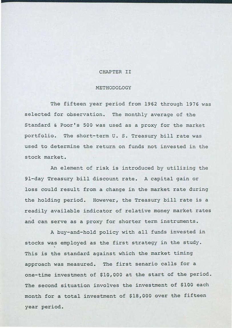
CHAPTER II
METHODOLOGY
The fifteen year period from 1962 through 1976 was
selected for observation. The monthly average of the
Standard & Poor's 500 was used as a proxy for the market
portfolio. The short-term U. S. Treasury bill rate was
used to determine the return on funds not invested in the
stock market.
An element of risk is introduced by utilizing the
91-day Treasury bill discount rate. A capital gain or
loss could result from a change in the market rate during
the holding period. However, the Treasury bill rate is a
readily available indicator of relative money market rates
and. can serve as a proxy for shorter term instruments.
A buy-and-hold policy with all funds invested in
stocks was employed as the first strategy in the study.
This is the standard against which the market timing
approach was measured. The first senario calls for a
one-time investment of $10,000 at the start of the period.
The second situation involves the investment of $100 each
month for a total investment of $18,000 over the fifteen
year period.
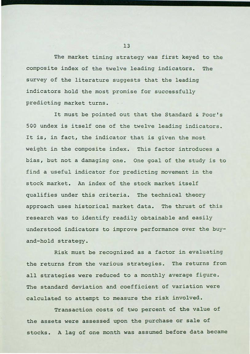
13
The market timing strategy was first keyed to the
composite index of the twelve leading indicators. The
survey of th~ literature suggests that the leading
indicators hold the most promise for successfully
predicting market turns.
It must be pointed out that the Standard & Poor's
500 undex is itself one of the twelve leading indicators.
It is, in fact, the indicator that is given the most
weight in the composite index. This factor introduces a
bias, but not a damaging one. One goal of the study is to
find a useful indicator for predicting movement in the
stock market. An index of the stock market itself
qualifies under this criteria. The technical theory
approach uses historical market data; The thrust of this
research was to identify readily obtainable and easily
understood indicators to improve performance over the buy
and-hold strategy.
Risk must be recognized as a factor in evaluating
the returns from the various strategies. The returns from
all strategies were reduced to a monthly average figure.
The standard deviation and coefficient of variation were
calculated to attempt to measure the risk involved.
Transaction costs of two percent of the value of
the assets were assessed upon the purchase or sale of
stocks. A lag of one month was assumed before data became

14
available. To compensate for this lag, the purchase or
sale price used was for the month following the purchase
or sale signal.
Dividends on stocks and interest on Treasury bills
were considered to roughly offset during rnost · of the
period and were not included in the calculations. An
adjustment was made for the period from 1969 to 1981,
when interest rates moved into the double-digit range.
Actually, rates on Treasury bills tended to far exceed
dividends on common stocks and would result in more
favorable results for the market timing strategies if
considered. The average dividend rates on the Standard &
Poor's 500 and the average discount rate on Treasury bills
were as follows:
Dividend Treasury Period Rates Bill Rates
1961-1963 2.14% 2.77% 1968-1970 3.13 6.16 1980-1981 5.77 12.85
The effect of taxes was not considered in the
study. The tax effect would be rather small for the
average investor. It can easily be added to the
calculations for the investor in a high tax bracket.
Conclusions were drawn from the fifteen-year base
period and applied to a five-year test period from 1977 to
1981. Again, a one-time investment of $10,000 and a
monthly investment of $100 were used to test the two
15
approaches.
The data was analyzed to determine whether or not
a shift between strategies would produce .better results
than pursuing a single approach for the whole period. An
attempt was then made to identify factors that would
correctly key such a change.

CHAPTER III
FINDINGS
Two decision rules were developed for a market
timing strategy that significantly outperformed the
buy-and-hold approach. Both of these decision rules
involve using the composite index of twelve leading
indicators.
The first and simplest of the successful
strategies calls for a purchase after two successive
monthly increases in the composite .index of twelve leading
indicators. Conversely, it calls for a sale after two
successive monthly decreases in the index. This ~ery
simple approach resulted in eight moves in and out of the
market, half of which were counter productive.
Nevertheless, . it was significantly better than merely
buying and holding stocks for the fifteen-year period.
A refinement of the first strategy provided for
significantly improved results. This approach called for
purchases or sales after two consecutive monthly positive
or negative changes in the composite index of twelve
leading indicators over three month spans. The smoothing
effect of this indicator resulted in fewer trades, five,
17
of which only one produced .unfavorable results.
The buy-and-hold strategy provided an increase of
$4,729 on the .original $10,000 investment • . Table 1 shows
the calculation . . This compares to an increase of $9,227
with the first market timing approach and $11,466 with the
second. These calculations are shown ~n Tables 2 and 4,
respectively. Neither .of these last two figures include
earnings in the money market while funds were held out of
the stock market.
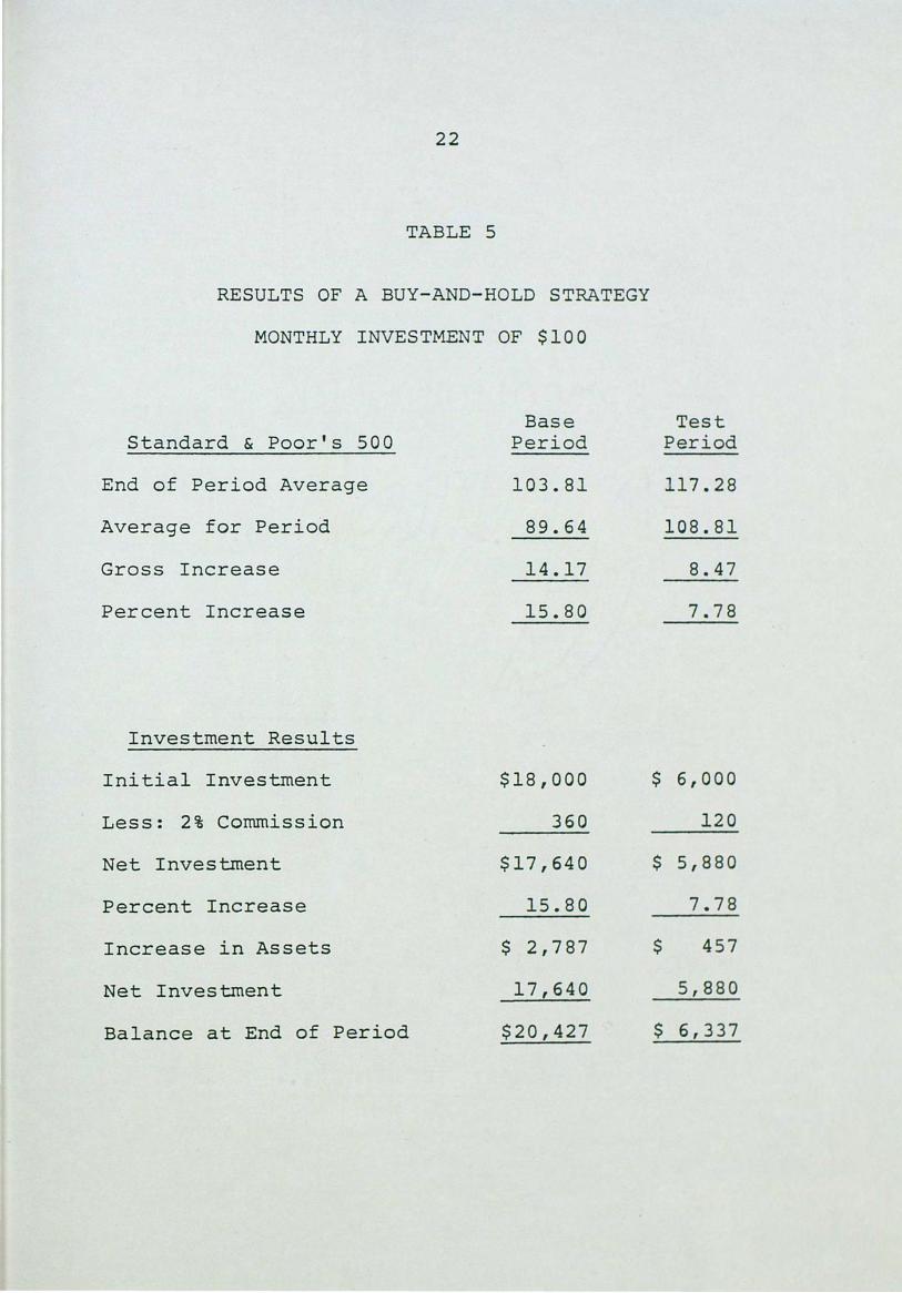
A second comparison was made of the various
strategies. This study involved an investment of $100
per month for the same fifteen-year . period. The total
investment of $18,000 resulted in a balance of $20,427
at the end of the period for the buy-and-hold alternative.
The increase was $2,427 as is shown in Table 5.
Both of the market timing strategies produced a
greater gain from stock market transactions than the buy
and-hold approach. The first of these strategies resulted
in an increase of $5,541, while the second yielded $6,245.
Tables 6 and 8 show these results. Thus, the overall
results of market timing are superior to the buy-and-hold
program.
The decision rules developed above were applied to
the test period. of 1977 through 1981. The results obtained
on stock market investments were not in keeping with the

18
TABLE 1
RESULTS OF A BUY-AND-HOLD STRATEGY
INITIAL INVESTMENT OF $10,000
Standard & Poor's 500
End of Period Average
Start of Period Average
Gross Increase
Percent Increase
Investment Results
Initial Investment
Less: 2% Commission
Net Investment
Percent Increase
Increase in Assets
Net Investment
Balance at End of Period
Base Period
103.81
69.07
34.74
50.30
$10,900
200
$ 9,800
50.30
$ 4,929
9,800
$14,729
Test Period
117.28
103.81
13.47
12.98
$10,000
200
$ 9,800
12.98
$ 1,272
9,800
$11,072

TA
BL
E
2
RE
SUL
TS
OF
MA
RK
ET
TIM
ING
ST
RA
TE
GY
#
1
INIT
IAL
IN
VE
STM
EN
T
OF
$1
0,0
00
BA
SE
PE
RIO
D
Buy
S&
P C
ash
2%
N
et
Sell
S&
P G
ain
S
ale
2%
D
ate
5
00
A
vail
ab
le
Fee
Inv
este
d
Date
5
00
(L
oss
) P
roceed
s F
ee
Sep
/62
:5
8.0
0
$1
0,0
00
$
20
0
$ 9
,80
0
Au
g/6
3
70
.98
2
2.3
7%
$
11
,99
2
$2
40
Oct/
62
7
3.0
3
11
,75
2
23
5
11
,51
7
Jun
/66
8
6.0
6
17
.84
1
3,5
72
2
71
~
\0
Mar
/67
8
9.4
2
13
,30
1
26
6
13
,03
5
Ap
r/6
9
10
1.2
6
13
.24
1
4,7
61
2
95
Jun
/70
7
5.5
9
14
,46
6
28
9
14
,17
7
Au
g/7
0
77
.92
3
.08
1
4,6
14
2
92
Oct/
70
8
4.3
7
14
,32
2
28
6
14
,03
6
Sep
/71
9
9.4
0
17
.81
1
6,5
36
3
31
No
v/7
1
92
.78
1
6,2
05
3
24
1
5,8
81
M
ay/7
3
10
7.2
2
15
.56
1
8,3
52
3
67
Dec
/73
9
4.7
8
17
,98
5
36
0.
17
,62
5
Feb
/74
9
3.4
5
(1.4
0)
17
,37
8
34
8
May
/75
9
0.1
0
17
,03
0
34
1
16
,68
9
Jan
/77
1
03
.81
1
5.2
1
19
,22
7

TA
BL
E
3
RE
SUL
TS
OF
MA
RK
ET
TIM
ING
ST
RA
TE
GY
#
1
INIT
IAL
IN
VE
STM
EN
T
OF
$1
0,0
00
TE
ST
P
ER
IOD
Buy
S&
P C
ash
2%
N
et
Sell
S&
P G
ain
S
ale
2%
D
ate
5
00
A
vail
ab
le
Fee
Inv
este
d
Date
5
00
(L
oss
) P
roceed
s F
ee
--
Sep
/77
9
6.2
3
$1
0,0
00
$
20
0
$ 9
,80
0
Mar/
79
1
00
.11
4
.03
%
$1
0,1
95
$
20
4
tv
Ju1
/79
1
02
.71
9
,99
1
20
0
9,7
91
S
ep
/79
1
08
.60
5
.73
1
0,3
52
2
07
0
Au
g/8
0
12
3.5
0
10
,14
5
20
3
9,9
42
F
eb
/81
1
28
.40
3
.97
1
0,3
37
2
07
May
/81
1
31
.73
1
0,1
30
2
03
9
,92
7
Ju1
/81
1
29
.13
{
1.9
7)
9,7
31
1
95
9,5
36

TA
BL
E
4
RE
SUL
TS
OF
MA
RK
ET
TIM
ING
ST
RA
TE
GY
#2
INIT
IAL
IN
VE
STM
EN
T
OF
$1
0,0
00
Bu
y
S&P
Cash
2%
N
et
Sell
S&
P G
ain
S
ale
2%
D
ate
5
00
A
vail
ab
le
Fee
Inv
este
d
Date
5
00
{
Lo
ss)
Pro
ceed
s F
ee
Base
P
eri
od
Sep
/62
5
8.0
0
$1
0,0
00
$
20
0
$ 9
,80
0
Jun
/66
8
6.0
6
48
.37
%
$1
4,5
40
$
29
1
Feb
/67
8
9.4
2
14
,24
9
28
5
13
,96
4
Ap
r/6
9
10
1.2
6
13
.24
1
5,8
13
3
16
N
.._,
Oct/
70
8
4.3
7
15
,49
7
31
0
15
,18
7
Sep
/71
9
9.4
0
17
.81
1
7,8
92
3
58
No
v/7
1
92
.78
1
7,5
34
3
51
1
7,1
83
Ju
n/7
3
10
4.7
5
12
.90
1
9,4
00
3
88
May
/75
9
0.1
0
19
,01
2
38
0
18
,63
2
Jan
/77
1
03
.81
1
5.2
1
21
,46
6
Test
Peri
od
Sep
/77
9
6.2
3
$1
0,0
00
$
20
0
$ 9
,80
0
Feb
/79
9
8.2
3
2.0
9%
$
10
,00
5
$2
00
Aug
-SO
1
23
.50
9
,80
5
19
6
9,6
09
Ju
1/8
1
12
9.1
3
4.5
5
10
,04
6
20
1
9,8
45
22
TABLE 5
RESULTS OF A BUY-AND-HOLD STRATEGY
MONTHLY INVESTMENT OF $100
Base Test Standard & Poor's 500 Period Period
End of Period Average 103.81 117.28
Average for Period 89.64 108.81
Gross Increase 14.17 8.47
Percent Increase 15.80 7.78
Investment Results
Initial Investment $18,000 $ 6,000
Less: 2% Corrunission 360 120
Net Investment $17,640 $ 5,880
Percent Increase 15.80 7.78
Increase in Assets $ 2,787 $ 457
Net Investment 17,640 5,880
Balance at End of Period $20,427 $ 6,337

TA
BL
E
6
RE
SUL
TS
OF
MA
RK
ET
TIM
ING
ST
RA
TE
GY
il
MO
NTH
LY
INV
EST
ME
NT
O
F $
10
0
BA
SE
PE
RIO
D
Buy
S&
P C
ash
2%
N
et
Sell
S&
P G
ain
S
ale
2%
C
ash
D
ate
5
00
A
vail
ab
le
Fee
Inv
este
d
Date
5
00
(L
oss
) P
roceed
s F
ee
Ad
ded
N
Sep
/62
5
8.0
0
$ 9
00
$
18
$
88
2
Au
g/6
3
70
.98
2
2.3
7%
$
1,0
79
$
22
$1
,30
0
w
Oct/
63
7
3.0
3
2,3
57
47
2
,31
0
Jun
/66
8
6.0
6
17
.84
2
,72
2
54
4,1
00
Mar/
67
8
9.4
2
6,7
68
1
35
,6
,63
3
Ap
r/6
9
10
1.2
6
13
.24
7
,51
1
15
0
3,9
00
Jun
/70
1
12
.61
1
1,2
61
2
25
1
1,0
36
A
ug
/70
7
7.9
2
3.0
8
11
,37
6
22
8
40
0
Oct/
70
8
4.3
7
11
,54
8
23
1
11
,31
7
Sep
/71
9
9.4
0
17
.81
1
3,3
33
2
67
1
,30
0
No
v/7
1
92
.78
1
4,3
66
2
87
1
4,0
79
M
ay/7
3
10
7.2
2
15
.56
1
6,2
70
3
25
2
,50
0
Dec/7
3
94
.78
1
8,4
45
3
69
1
8,0
76
F
eb
/74
9
3.4
5
(1.4
0)
17
,82
3
35
6
1,7
00
May
/75
9
0.1
0
19
,16
7
38
3
18
,78
4
Jan
/77
1
03
.81
1
5.2
1
21
,64
1
-1
,90
0
23
,54
1

TA
BL
E
7
RE
SUL
TS
OF
MA
RK
ET
TIM
ING
ST
RA
TE
GY
#
1
MO
NTH
LY
INV
EST
ME
NT
O
F $
10
0
TE
ST
P
ER
IOD
Buy
S&
P C
ash
2%
N
et
Sell
S&
P G
ain
S
ale
2%
C
ash
D
ate
5
00
A
vail
ab
le
Fee
Inv
este
d
Date
5
00
(L
oss
) P
roceed
s F
ee
Ad
ded
N
Sep
/77
9
6.2
3
$ 9
00
$
18
$
88
2
Mar/
79
1
00
.11
4
.03
%
$ 9
18
~
$ 1
8
$2
,20
0
Ju
l/7
9
10
2.7
1
3,1
00
6
2
3,0
38
S
ep
/79
1
08
.60
5
.73
3
,21
2
64
1
,30
0
Au
g/8
0
12
3.5
0
4,4
48
89
4
,35
9
Feb
/81
1
28
.40
3
.97
4
,53
2
91
9
00
May
/81
1
31
.73
5
,34
1
10
7
5,2
34
Ju
l/8
1
12
9.1
3
(1.9
7)
5,1
31
1
03
7
00
5,7
28

\
TA
BL
E
8
RE
SUL
TS
OF
MA
RK
ET
TIM
ING
ST
RA
TE
GY
#
2
MO
NTH
LY
INV
EST
ME
NT
O
F $
10
0
Buy
S&
P C
ash
2%
N
et
Sell
S&
P G
ain
S
ale
2%
C
ash
D
ate
5
00
A
vail
ab
le
Fee
Inv
este
d
Date
5
00
(L
oss
) P
roceed
s F
ee
Ad
ded
Bas
e P
eri
od
t\
..)
Sep
/62
5
8.0
0
$ 9
00
$
18
$
88
2
Jun
/66
8
6.0
6
48
.37
%
$ 1
,30
9
$ 2
6
$5
,30
0
Ul
Feb
/67
8
9.4
2
6,5
83
1
32
6
,45
1
Ap
r/6
9
10
1.2
6
13
.24
7
,30
5
14
6
4,4
00
Oct/
70
8
4.3
7
11
,55
9
23
1
.1,1
,328
S
ep
/71
9
9.4
0
17
.81
1
3,3
46
2
67
1
,30
0
No
v/7
1
92
.78
1
4,3
79
2
88
1
4,0
91
Ju
n/7
3
10
4.7
5
12
.90
1
5,9
09
3
18
4
,20
0
May
/75
9
0.1
0
19
,79
1
39
6
19
,39
5
Jan
/77
1
03
.81
1
5.2
1
22
,34
5
-1
,90
0
24
,24
5
Test
Peri
od
Sep
/77
9
6.2
3
$ 9
00
$
18
$
88
2
Feb
/79
9
8.2
3
2.0
9
$ 9
00
$
18
$
3,5
00
Au
g/8
0
12
3.5
0
4,3
82
8
8
4,2
94
Ju
1/8
1
12
9.1
3
4.5
5
4,4
89
89
1
,60
0
6,0
00
26
base period. The buy-and-hold strategy outperformed both
market timing strategies.
Table 1 shows an increase of $1,072 for the buy
and-hold approach. Market timing strategy number one
resulted .in a loss of $464 for the five years, while
strategy number two produced a loss of $155. These
results are shown in Tables 3 and 4.
The first market timing strategy called for
investment in the money market from January, 1977 to
September, 1977; March, 1979 to July, _ 1979; September,
1979 to August, 1980; February, 1981 to May, 1981; and
July, 1981 to the end of the period. The average interest
rate for these thirty-two months was 9.86%. The dividend
yield was under 5%. Therefore, a superior return of more
than 5% in the money market would add some $1,350 to
offset the $464 loss from the stock market for a net ga1n
of $886.
A similiar adjustment for the second strategy
would add some $1,350 of money market earnings to offset
the $155 loss in the stock market and result in a net gain
of $1,195. The difference between a buy-and-hold strategy
and either market timing approach was not significant
during the test period. Perhaps a key to the disappointing
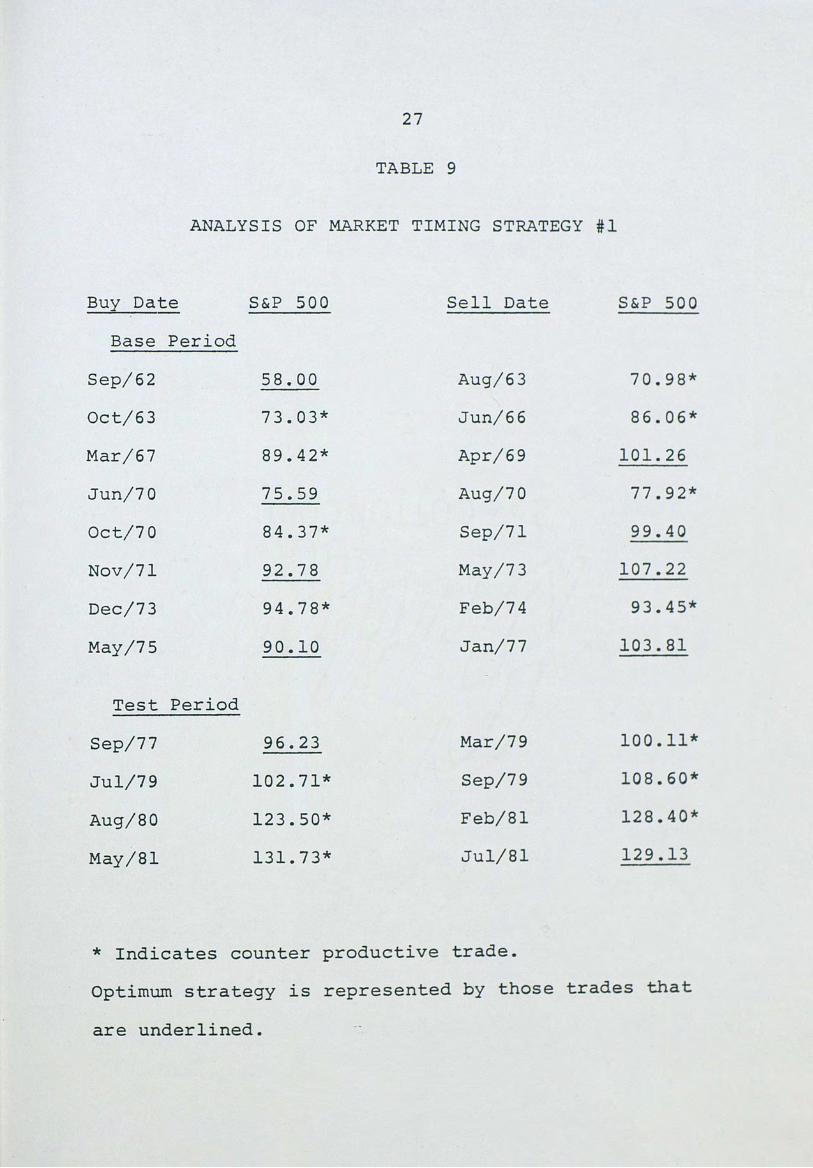
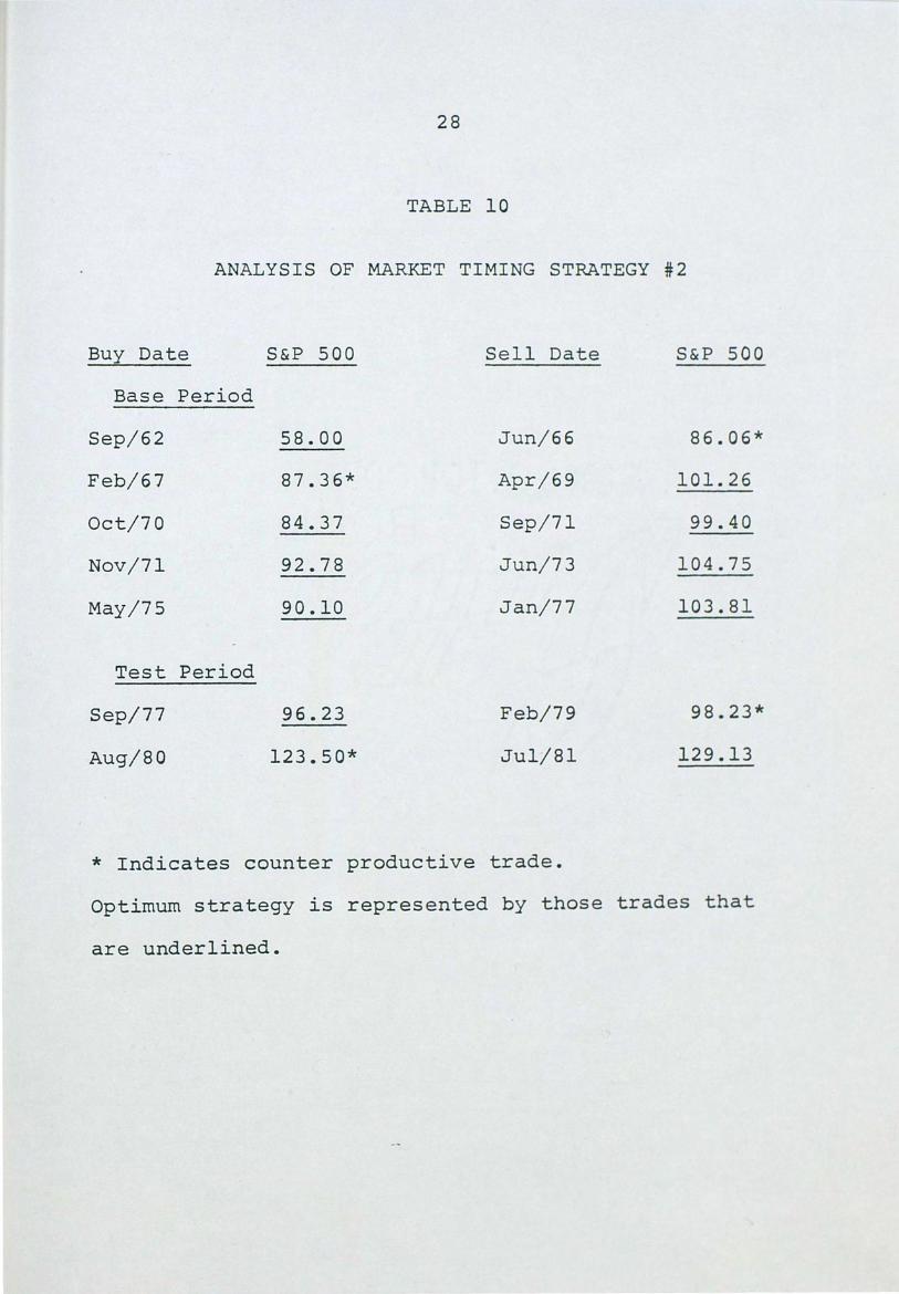
results for market timing can be found 1n Tables 9 & 10.
The tables show that four moves were made in and
27
TABLE 9
ANALYSIS OF MARKET TIMING STRATEGY #1
Buy Date S&P 500 Sell Date S&P 500
Base Period
Sep/62 58.00 Aug/63 70.98*
Oct/63 73.03* Jun/66 86.06*
Mar/67 89.42* Apr/69 101.26
Jun/70 75.59 Aug/70 77.92*
Oct/70 84.37* Sep/71 99.40
Nov/71 92.78 May/73 107.22
Dec/73 94.78* Feb/74 93.45*
May/75 90.10 Jan/77 103.81
Test Period
Sep/77 96.23 Mar/79 100.11*
Ju1/79 102.71* Sep/79 108.60*
Aug/80 123.50* Feb/81 128.40*
May /81 131.73* Ju1/81 129.13
* Indicates counter productive trade.
Optimum strategy is represented by those trades that
are underlined.
28
TABLE 10
ANALYSIS OF MARKET TIMING STRATEGY #2
Buy Date
Base Period
Sep/62
Feb/67
Oct/70
Nov/71
May/75
Test Period
Sep/77
Aug/80
S&P 500
58.00
87.36*
84.37
92.78
90.10
96.23
123.50*
Sell Date
Jun/66
Apr/69
Sep/71
Jun/73
Jan/77
Feb/79
Jul/81
* Indicates counter productive trade.
S&P 500
86.06*
101.26
99.40
104.75
103.81
98.23*
129.13
Optimum strategy is represented by those trades that
are underlined.

29
out of the stock market during the test period under the
first market timing strategy. Three of these moves, or
75% of the total, were counter productive. One of the two
moves called for under the second market timing strategy
was counter productive, a 50% failure rate. If some or all
of these transactions could be eliminated by keying a
change in strategy at the appropriate time, the results
should be substantially improved.
Looking at the entire twenty-year span that
encompasses both the base and test periods, the buy-and
hold strategy prod.uced the best results through April,
1979. The market timing strategies were vastly superior
from April, 1969 to September, 1977. The period from
September, 1977 to July, 1981 again called for the buy
and-hold alternative. Finally, one would be well advised
to switch to the market timing approach at July, 1981.
These few adjustments make for dramatic improvements in
performance.
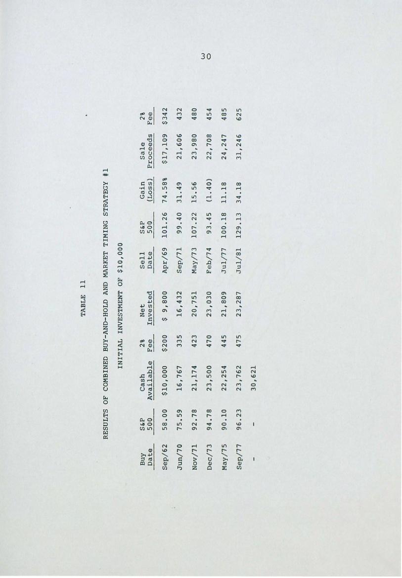
The combination of buy-and-hold with the first
market timing strategy resulted in a return of $20,621 on
the initial $10,000 investment. The same approach returns
$12,505 on a $100 per month investment over the twenty-year
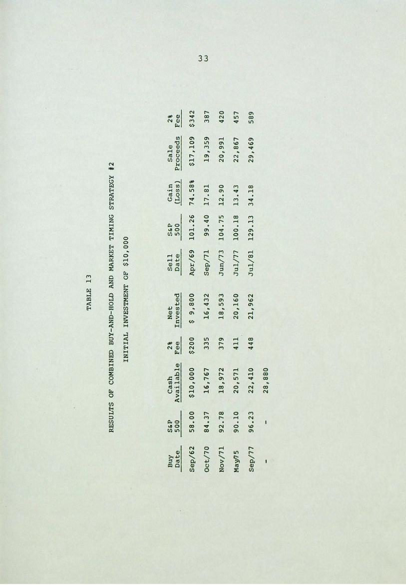
period. Tables 11 and 12 show these results.
The second market timing strategy, when alternated
with buy-and-hold, returned $18,880 on the original
TA
BL
E
11
RE
SUL
TS
OF
CO
MB
INE
D
BU
Y-A
ND
-HO
LD
A
ND
M
AR
KET
T
IMIN
G
STR
AT
EG
Y
#1
INIT
IAL
IN
VE
STM
EN
T
OF
$1
0,0
00
Buy
S&
P C
ash
2%
N
et
Sell
S&
P G
ain
S
ale
2%
D
ate
5
00
A
vail
ab
le
Fee
Inv
este
d
Date
5
00
(L
oss
) P
roceed
s F
ee
-
Sep
/62
5
8.0
0
$1
0,0
00
$
20
0
$ 9
,80
0
Ap
r/6
9
10
1.2
6
74
.58
%
$1
7,1
09
$
34
2
Ju
n/7
0
75
.59
1
6,7
67
3
35
1
6,4
32
S
ep
/71
9
9.4
0
31
.49
2
1,6
06
4
32
No
v/7
1
92
.78
2
1,1
74
4
23
2
0,7
51
M
ay/7
3
10
7.2
2
15
.56
2
3,9
80
4
80
W
· D
ec/7
3
94
.78
2
3,5
00
4
70
2
3,0
30
F
eb
/74
9
3.4
5
(1.
40
) 2
2,7
08
4
54
0
May
/75
9
0.1
0
22
,25
4
44
5
21
,80
9
Ju
l/7
7
10
0.1
8
11
.18
2
4,2
47
4
85
Sep
/77
9
6.2
3
23
,76
2
47
5·
23
,28
7
Ju
l/8
1
12
9.1
3
34
.18
3
1,2
46
6
25
30
,62
1

TA
BL
E
12
RE
SUL
TS
OF
CO
MB
INED
B
UY
-AN
D-H
OL
D
AN
D
MA
RK
ET
TIM
ING
ST
RA
TE
GY
#
1
MO
NTH
LY
INV
EST
ME
NT
O
F $
10
0
Buy
S&
P C
ash
2%
N
et
Sell
S&
P G
ain
S
ale
2%
C
ash
D
ate
5
00
A
vail
ab
le
Fee
Inv
este
d
Date
5
00
(L
oss
) P
roceed
s F
ee
Ad
ded
--
Sep
/62
5
8.0
0
$ 9
00
$
18
$
88
2
Ap
r/6
9
10
1.2
6
74
.58
%
$ 1
,54
0
$ 3
1
$9
,30
0
Jun
/70
7
5.5
9
10
,80
9
21
6
10
,59
3
Sep
/71
9
9.4
0
31
.49
1
3,9
29
2
79
1
,70
0
No
v/7
1
92
.78
1
5,3
50
3
07
1
5,0
43
M
ay/7
3
10
7.2
2
15
.56
1
7,3
84
3
48
2
,50
0
w ~
Dec/7
3
94
.78
1
9,5
36
3
91
1
9,1
45
F
eb
/74
9
3.4
5
(1.4
0)
18
,87
7
37
6
1,7
00
May
/75
9
0.1
0
20
,20
1
40
4
19
,79
7
Ju1
/77
1
00
.18
1
1.1
8
22
,01
0
44
0
2,8
00
Sep
/77
9
6.2
3
24
,37
0
48
7
23',
88
3
Ju
l/8
1
12
9.1
3
34
.18
3
2,0
46
6
41
5
,10
0
36
,50
5
32
investment of $10,000. The monthly investment of $100
returned $11,889 at the end of twenty years. These
figures are shown in Tables 13 and 14. Approximately
$1,000 in money market earnings can be added to all four
of the returns shown above for comparison with the
previous market timing results.
These combined strategies must be compared with
the entire twenty-year period under examination, which is
composed of the base period and the test period. The
buy-and-hold strategy would show a return of $6,640 on
the $10,000 investment and $5,207 on the $100 per month
investment. The first market timing strategy returned
$9,343 on $10,000 and $6,056 on the ~onthly investment
program. The figures for the second market timing
strategy were $12~790 and $8,097, respectively. Thus,
trerewards are great for a timely changing of strategy.
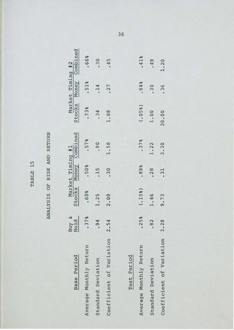
The introduction of risk into the study was
accomplished by calculating the standard deviation for
each of the basic strategies, both during the base period
and the test period. The calculations were made only for
the $10,000 investment program. The results were rather
surprising.
The first market timing strategy shows a greater
return, adjusted for transaction costs, than the buy-and
hold strategy. It shows comparable risk during the base
Buy
D
ate
Sep
/62
Oct/
70
No
v/7
1
Ma~5
Sep
/77
TA
BL
E
13
RE
SUL
TS
OF
CO
MB
INED
B
UY
-AN
D-H
OL
D
AN
D
MA
RK
ET
TIM
ING
ST
RA
TE
GY
#2
INIT
IAL
IN
VE
STM
EN
T
OF
$1
0,0
00
S&P
Cash
2%
N
et
Sell
S&
P G
ain
S
ale
5
00
A
vail
ab
le
Fee
Inv
este
d
Date
5
00
(L
oss
) P
roceed
s --
58
.00
$
10
,00
0
$2
00
$
9,8
00
A
pr/
69
1
01
.26
7
4.5
8%
$
17
,10
9
84
.37
1
6,7
67
3
35
1
6,4
32
S
ep
/71
9
9.4
0
17
.81
1
9,3
59
92
.78
1
8,9
72
3
79
1
8,5
93
Ju
n/7
3
10
4.7
5
12
.90
2
0,9
91
90
.10
2
0,5
71
4
11
2
0,1
60
Ju
1/7
7
10
0.1
8
13
.43
2
2,8
67
96
.23
2
2,4
10
4
48
2
1,9
62
Ju
1/8
1
12
9.1
3
34
.18
2
9,4
69
28
,88
0
2%
Fee
$3
42
w
3
87
w
42
0
45
7
58
9

TA
BL
E
14
RE
SUL
TS
OF
CO
MB
INED
B
UY
-AN
D-H
OL
D
AN
D
MA
RK
ET
TIM
ING
ST
RA
TE
GY
#2
MO
NTH
LY
INV
EST
ME
NT
O
F $
10
0
Buy
S&
P C
ash
2%
N
et
Sell
S&
P G
ain
S
ale
2%
C
ash
D
ate
5
00
A
vail
ab
le
Fee
Inv
este
d
Date
5
00
~oss)
Pro
ceed
s F
ee
Ad
ded
Sep
/62
5
8.0
0
$ 9
00
$
18
$
88
2
Ap
r/6
9
10
1.2
6
74
.58
%
$ 1
,54
0
$ 3
1
$9
,70
0
Oct/
70
8
4.3
7
11
,20
9
22
4
10
,98
5
Sep
/71
9
9.4
0
17
.81
1
2,9
41
2
59
1
,30
0
No
v/7
1
92
.78
1
3,9
82
2
80
1
3,7
02
Ju
n/7
3
10
4.7
5
12
.90
1
5,4
70
3
09
4
,20
0
w ~
May
/75
9
0.1
0
19
,36
1
38
7
18
,97
4
Ju1
/77
1
00
.18
1
3.4
3
21
,52
2
43
0
2,8
00
Sep
/77
9
6.2
3
23
,89
2
47
8
23
,41
4
Ju1
/81
1
29
.13
3
4.1
8
31
,41
7
62
8
5,1
00
35
,88
9

35
period and higher risk during the test period. The return
relative to risk is much greater for the market timing
strategy during the base period and roughly equivalent
during the test period. Table 15 shows the results.
The second market timing strategy shows a greater
return and a lower risk than the buy-and-hold approach.
This is the case during the base period and the test
period. If one must choose a single strategy and hold to
it, the second market timing strategy is clearly the one.
The first market timing strategy is slightly superior if
one can move between basic strategies on a timely basis.
It does involve significantly greater risk than is
justified by the return.
The results shown in Table 15 are felt to be
reliable on the basis of their t ratios. The t ratios
were as follows:
Buy-and-Hold/ Market Timing #1
Market Timing #1/ Market Timing #2
Buy-and-Hold/ Market Timing #2
Base Period
.58
.37
1.16
Test Period
.21
.08
.35
TA
BL
E
15
AN
AL
YSI
S O
F R
ISK
A
ND
R
ETU
RN
Buy
&
M
ark
et
Tim
ing
#l
. M
ark
et
Tim
in9
: #2
B
ase
P
eri
od
H
old
S
tock
s M
on
ey
Co
mb
ined
S
tock
s M
oney
C
om
bin
ed
--
Av
era
ge
Mo
nth
ly
Retu
rn
.37
%
.60%
.5
0%
.5
7%
.7
3%
.51%
.6
6%
Sta
nd
ard
D
ev
iati
on
.9
4
1.2
5
.15
.9
0
.34
.1
4
.30
Co
eff
icie
nt
of
Vari
ati
on
2
.54
2
.08
.3
0
1.5
8
1.8
8
.27
.4
5
w
0)
Test
Peri
od
Av
era
ge
Mo
nth
ly
Retu
rn
.25%
( .
15%
)'
.89%
.3
7%
(.0
5%
) .8
4%
.41%
Sta
nd
ard
D
ev
iati
on
.8
2
1.4
6
.28
1
.22
1
.00
.3
0
.49
Co
eff
icie
nt
of
Vari
ati
on
3
.28
9
.73
.3
1
3.3
0
20
.00
.3
6
1.2
0

CHAPTER IV
CONCLUSIONS
The returns to be obtained from an investment
program that moves back and forth between two different
strategies at the appropriate time are quite impressive.
Two easily applied decision rules have been established
for the market timing phase of the program. These rules
do not pretend to signal market peaks or troughs. They
did supply results superior to the basic buy-and-hold
strategy. They are objective rules that require no
judgement call on the part of the investor.
The problem then becomes one of determining in
advance when to switch basic strategies. Changes in
strategy were called for in 1969, 1977 and 1981. It had
been suggested that changes in the political scene might
call for changes in investment strategy. This lead to the
observation that 1969 was the first year in office of a
Republican President, 1977 was the first year in office of
a Democrat President, . and 1981 was the first year in office
of a Republican President. Thus, a change in investment
strategy is apparently called for whenever there is a
change in political parties in the White House.
The appropriate investment strategy under the

38
Democrats (1962-1968 and 1977-1980) is to buy-and-hold.
The appropriate investment strategy under the Republicans
(1969-1976 and 1981 to the present) is market timing.
A possible explanation for this observation is
that the investing public perceives the Democrat
administrations as inflationary in nature. Presidents
Johnson (guns and butter) and Carter (double-digit
inflation) did nothing to dispell this notion. The
investing public perceives the Republican administrations
as anti-inflationary in nature. Presidents Nixon (wage
and price controls), Ford (Whip Inflation Now), and
Reagan (single-digit inflation) have done nothing to
dispell this notion. This perception alone seems enough
to trigger a change in investment philosophy.
If the investing public anticipates continued
inflation, it remains fully invested in stocks. If it does
not anticipate continued inflation, it is indecisive in its
investment strategy. The stock market will therefore be
more volatile and a strategy of market timing will be more
appropriate. While these may be subjective conclusions,
they are supported by the results of this study. It will
be interesting to see if they hold true in the future. At
the time of this writing, a market timing strategy is
called for and the leading indicators are signaling for
a move into the stock market.

39
SELECTED BIBLIOGRAPHY
Dreman, David. Contrarian Investment Strategy. New York: Random House, 1979.
Heathcotte, . Bryan, and Apilado, Vincent P. "The Predictive Content of Some Leading Economic Indicators for Future Stock Prices," Journal of Financial and Quantitative Analysis 9 (March, 1974): 247-258.
Malkiel, Burton G. A Random Walk Down Wall Street. New York: W. W. Norton & Co., 1973.
Markowitz, Harry. "Portfolio Selection," Journal of Finance 7 (March, 1952): 77-91.
Reilly, Frank K. Investment Analysis and Portfolio Management. Hinsdale IL: Dryden Press, 1979.
Rolo, Charles J. Gaining on the Market. Boston: Little, Brown and Company, 1982.
Rozeff, M. s. "The Money Supply and the Stock Market," Financial Analysts Journal 31 (September-October, 1975): 18-26.
Sharpe, William F. Portfolio Theory and Capital Markets. New York: McGraw-Hill, Inc., 1970 •
• "Likely Gains from Market Timing," Financial ---~-Analysts Journal 31 (March-April, 1975): 60-69.
Train, John. The Money Masters. New York: Harper & Row, 1980.