Brigham Young UniversityBYU ScholarsArchive

All Theses and Dissertations

1968-08-02

An Analysis and Comparison of Linear PhaseBandpass FiltersDarrell L. AshBrigham Young University - Provo

Follow this and additional works at: https://scholarsarchive.byu.edu/etd

Part of the Electrical and Computer Engineering Commons

This Thesis is brought to you for free and open access by BYU ScholarsArchive. It has been accepted for inclusion in All Theses and Dissertations by anauthorized administrator of BYU ScholarsArchive. For more information, please contact scholarsarchive@byu.edu, ellen_amatangelo@byu.edu.

BYU ScholarsArchive CitationAsh, Darrell L., "An Analysis and Comparison of Linear Phase Bandpass Filters" (1968). All Theses and Dissertations. 7072.https://scholarsarchive.byu.edu/etd/7072

AN ANALYSIS AND COMPARISON OF LINEAR

PHASE BANDPASS FILTERS

I

A Thesis

Presented to the Department of Electrical Engineering Science

Brigham Young University

In Partial Fulfillment

of the Requirements for the Degree

Master of Science

byDarrell L. Ash August 1908

ii

This thesis by Darrell L» Ash is accepted in its present form

by the Department of Electrical Engineering Science of Brigham loung

University as satisfying the thesis requirement for the degree of Master of Science.

LeM-t-DATE

Typed by Gail Bell

iii

VITA

The author was b o m near New Albany, Indiana, in 19^+• He attended high school in Corydon, Indiana, where he became the president

of the Senior Class and graduated with honors in 1962, After graduation from high school, he attended Evansville College (now known as the

University of Evansville) in Evansville, Indiana, where he was given

membership in several scholastic honorary fraternities, among which was Phi Kappa Phi, Later, he also joined the IEEE, While in under­graduate school, he participated in a cooperative engineering training

program offered by the college both as a means of livelihood and as a means of gaining practical experience in electronics. He obtained his BSEE from Evansville in May, 1967. In April, 1967, he received an NSF

Traineeship to do work for his Master's Degree at Brigham Young University,

ACKNOWLEDGEMENT

The author wishes to express his appreciation for the patient

counsel given him while working on this paper by Dr. DeVerl Humpherys

of the engineering staff at Brigham Young University, Without his help, this paper would not have been possible.

TABLE OF CONTENTS

v

CHAPTER PAGE

I. INTRODUCTION TO THE PROBLEM.............................. 1II. LOW-PASS PROTOTYPE ...................................... 2

Ideal Frequency Domain Filter . . . . . . . . . . . . . 2

Ideal Bandpass Filters and the IFDF ................... 4III. APPROXIMATIONS TO THE IFDF AND IDEAL BANDPASS FILTER . . . 6

Butterworth* s Maximally Flat Amplitude

Approximation .. ........ . . . . . . . . . . . . . 6Chebyshev*s Equal-Ripple Amplitude Approximation. . . . 9Maximally Flat Delay Approximation, . . . . . . . . . . 13

Disadvantages of these Approximations . . . . . . . . . 16

IV. LERNER'S BANDPASS FILTER APPROXIMATION .................. 18Infinite Network Approximation. . . . . . . . . . . . . 18

Truncation of the Infirite Network. . . . . . . . . . . 22V. REALIZATION AND ANALYSIS OF LERNER'S BANDPASS FILTER

APPROXIMATION. ........................................ 28Method of Realization 28

Seventh Order Lerner Realization, . . . . . . . . . . 30Analysis of Realized Lerner Filters . . . . . . . . . . JM-

Lerner Filters of Orders ?, 8, 9» and 11. . . . . . . 3^

vi

CHAPTER PAGE

Effects on Lemer's Approximation ofIncreasing the Bandwidth., . . . . . . . . . . . . 38

Effect of Inductance Errors 39

Effects of Resonant Frequency Errors, . . . . . . . . ^5Effects of Varying the Load and SourceResistances ........... . . . . . . . 8

Effects of Using Lossy Coils, • .................... 48Effects of Omitting the Corrector . 52Effects of Omitting the Correctors Yq. and Y ^ . . . 53Effects of Adding Out-of-Band Zeros , .............. 53

Final Comments on Lerner's Approximation . . 56VI. THE BENNETT LINEAR PHASE APPROXIMATION .................. 60

Theory and Method of Realization . . . . . . . . . . . 60

Realization and Analysis , . ........ . . . . . . . . 63Final Comments on Bennett’s Approximation 67

VII. LINEAR PHASE AND MAGNITUDE RELATIONSHIPS IN A LATTICENETWORK.......................................... 68Determination of the Relationships. . . . . . . . . . . 68Determination of Lattice Transfer Function from .Fifth

Order Chebyshev Linear Phase Approximation........ 73Experiments with Producing a Good IFDF Approximation

Using the Observed Phase and MagnitudeRelationships , . .......... . . . . . . . . . . . . 77

VIII. CONCLUSIONS. . . . . . ................................... 87

CHAPTER

vii

PAGE

BIBLIOGRAPHY APPENDIX . .

. . 89

. . 90

viii

LIST OF FIGURES

FIGURE PAGE

la. Magnitude and Phase Response of the IFDF . . . . . . . . . . 3lb. Impulse Response of the I F D F........ . 3

2. Positive Passband and Its Conjugate Image, . . . . . . . . . 53. Shifting the IFDF to Obtain a Bandpass Filter, . . . . . . . 34. Butterworth Approximation to the IFDF. .................. 85. Pole Arrangement of Butterworth Passband Shifted to U>e . , , 86. Low-Pass to Bandpass Transformations 10

7. Chebyshev Polynomials. • • * • * • • • * • • • • • • • * • « 108. Amplitude Response of Chebyshev Low-Pass Filter, .......... 129. Chebyshev Bandpass Filter Approximation............... 1210, Deviations from the Ideal Using a Maximally Flat Delay

Approximation. . . . 1511, Lattice Networks 1912, S-Plane Pole Pattern , f , . . . . . . . . . . . . . . . . . 2013« Circuit Form of and Ig, ................................. 2114, Division of the Branch Admittances . • • • • • ............ 2115, Transformation of Lattice, • • • • • • • • . . . • . * • , » 2416, Plot of the Admittance Xb* . . . . . . . . . . . . . . . . . 2417, Nine-Pole Filter 26

ix

FIGURE PAGE

18, Circuit Form of the Individual Arm Resonances. ............ 2919, Ya and Yg Pole Locations............ . 3220, Lemer Seventh Order Filter Network................. 33

21a, Calculated Magnitude Characteristics of Lemer Filters . . . 3521b, Calculated Group Delay Characteristics of Lemer Filters • . 36

22a, Lemer Filter Attenuation N = ? & 11, 30# Bandwidth...... **0

22b, Lemer Filter Group Delay N = 7 & 11, 30# Bandwidth, , , , , ^123a, Lemer Filter Attenuation N = 7 & 9, 10# L Errors, . . . • , ^3

23b, Lemer Filter Group Delay N = 7 & 9, 10# L Errors, , , , , , ^24a, Lemer Filter Attenuation N = 7 & 9, 5# Res, Freq, Errors, . **624b, Lemer Filter Group Delay N = 7 & 9, 5# Res, Freq, Errors, , 7

25a, Lemer Filter Attenuation N = 7, 1,0 ohm Coil Resistance . . 5025b, Lemer Filter Group Delay N = 7, H O ohm Coil Resistance , , 5126a, Lemer Filter Attenuation N = 9 & H » No Yq 5^

26b, Lemer Filter Group Delay N = 9 & 11, No Yc , , , , , , , , 5527a, Lemer Filter Attenuation, Out-of-Band Zeros at 0,950 X 10^

and 1,050 X 106 rps. and at 0,973 X 105 and1.027 X 106 rps........................................ .. 5?

27b, Lemer Filter Group Delay with Out-of-Band Zeros 5828a0 Bennett Realizations from Chebyshev Linear Phase Functions,

Magnitude Characteristics, 6528b, Bennett Realizations from Chebyshev Linear Phase Functions,

Group Delay. 6629, Third Order Thomson Filter Realization ?030a, Magnitude Characteristics of Thomson 3rd Order Realization , 71

X

figure page

30b, Group Delay of Thomson 3rd Order Realization 7231a, Chebyshev Linear Phase Approximations, 7531b. Chebyshev Linear Phase Approximations.......... 7632a. Chebyshev Fifth Order Function with Last Pole Moved Toward

juJAxis..................... , 7832b, Chebyshev Fifth Order Function with Last Pole Moved Toward

jUJAxis...................... 7933* Realization of Yg, , , , , ......... . . . . . . . . . . . . 8234. Realization of Y^. . . . . . . . . . ............ 8235. Fifth Order Chebyshev Approximation with Corrector

Resonance, • • • • « . « * • • .......... .. . ........... 84

36a. Fifth Order Chebyshev Linear Phase Filter with CorrectorResonance. 85

36b, Fifth Order Chebyshev Linear Pnase Filter with Corrector

Resonance, .......................... • . . .............. 80

CHAPTER I

INTRODUCTION TO THE PROBLEM

The ideal bandpass filter is defined as one which uniformly attenuates and delays all frequency components within the passband and effects zero transmission of all components outside the passband.For reasons which will be subsequently discussed, it is impossible to realize a stable lumped-element filter having this ideal characteristic.

This has made it necessary to find ways to physically approximate such a characteristic. Some of the more widely used methods will be com­

pared and analyzed in this paper.Among the methods which will be discussed and compared are the

Chebyshev, Butterworth, Thomson, Lerner, and Bennett approximations.

The functions possessing linear phases will be realized in lattice form, analyzed, and compared. In addition to analyzing and comparing these known approximations, an attempt will be made to develop new

approximations to the ideal bandpass filter by determining the relation­ships, if any, between a linear phase and the resulting magnitude in a lattice network. Such a relationship, if found, will be applied to the

task of developing a new approximation to the ideal bandpass filter.

CHAPTER II

LOW-PASS PROTOTYPE

I. IDEAL FREQUENCY DOMAIN FILTER

The low-pass prototype of the ideal bandpass filter is the

ideal frequency domain filter, abbreviated IFDF in the following

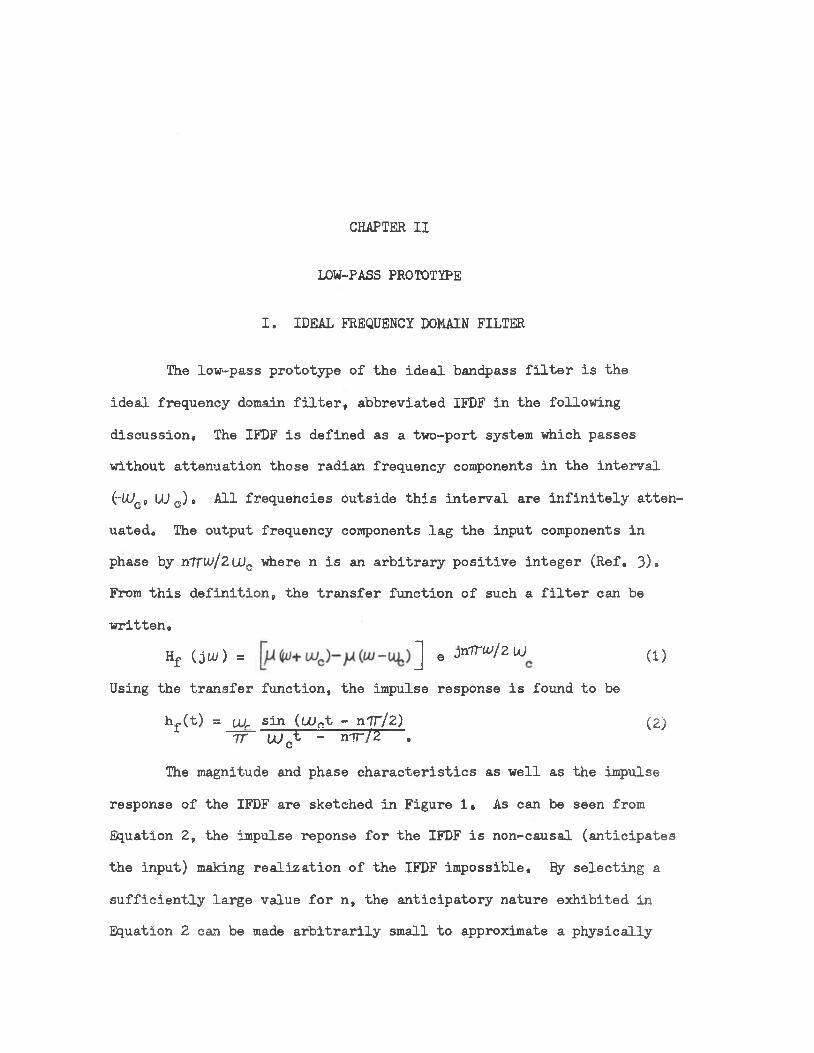
discussion. The IFDF is defined as a two-port system which passes without attenuation those radian frequency components in the interval

(-UJC, UJ c) o All frequencies outside this interval are infinitely atten­uated, The output frequency components lag the input components in phase by n'TTU)/2LUC where n is an arbitrary positive integer (Ref, 3)« From this definition, the transfer function of such a filter can be written.

Hf (ju/) = J e 3n'rruJ/Z UJ

Using the transfer function, the impulse response is found to be

hp(t) = at sin (C0Pt - n'TT/Z) f tt tuc£ - m r /2— .

(i)

(2)

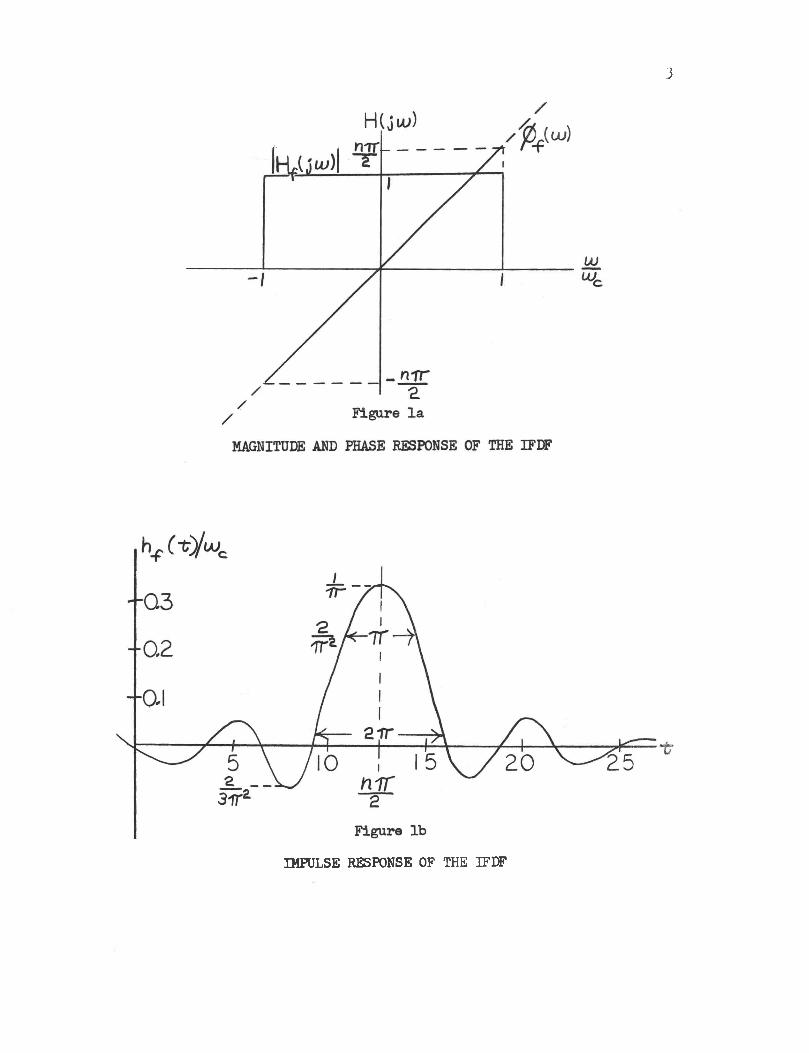
The magnitude and phase characteristics as well as the impulse

response of the IFDF are sketched in Figure 1, As can be seen from Equation 2, the impulse reponse for the IFDF is non-causal (anticipates

the input) making realization of the IFDF impossible. By selecting a sufficiently large value for n, the anticipatory nature exhibited in Equation 2 can be made arbitrarily small to approximate a physically

3

IMPULSE RESPONSE OF THE IFDF

4

realizable causal system. Since each reactive element in a filter net-

work can contribute a maximum phase change of ±TT/2 radians, the integer n is a rough indication of the number of reactive components required

for such an approximate realization of the IFDF (Ref. 3)•

II. IDEAL BANDPASS FILTERS AND THE IFDF

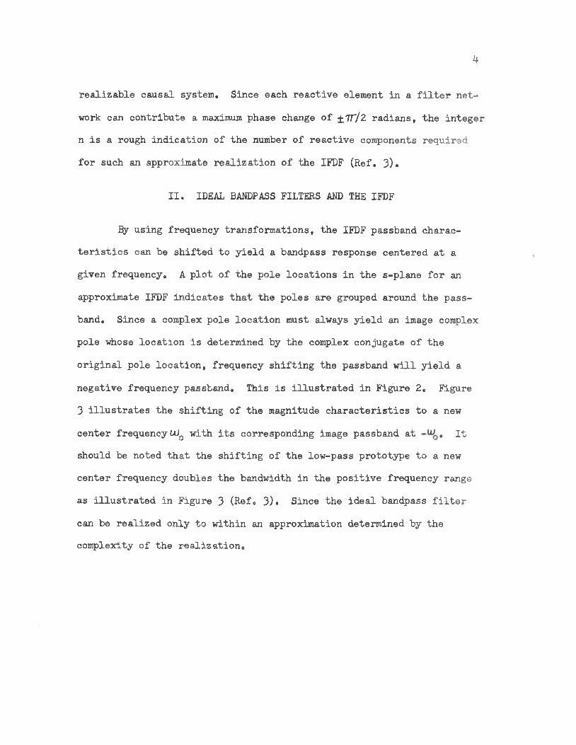
By using frequency transformations, the IFDF passband charac­teristics can be shifted to yield a bandpass response centered at a given frequency. A plot of the pole locations in the s-plane for an

approximate IFDF indicates that the poles are grouped around the pass- band. Since a complex pole location must always yield an image complex pole whose location is determined by the complex conjugate of the

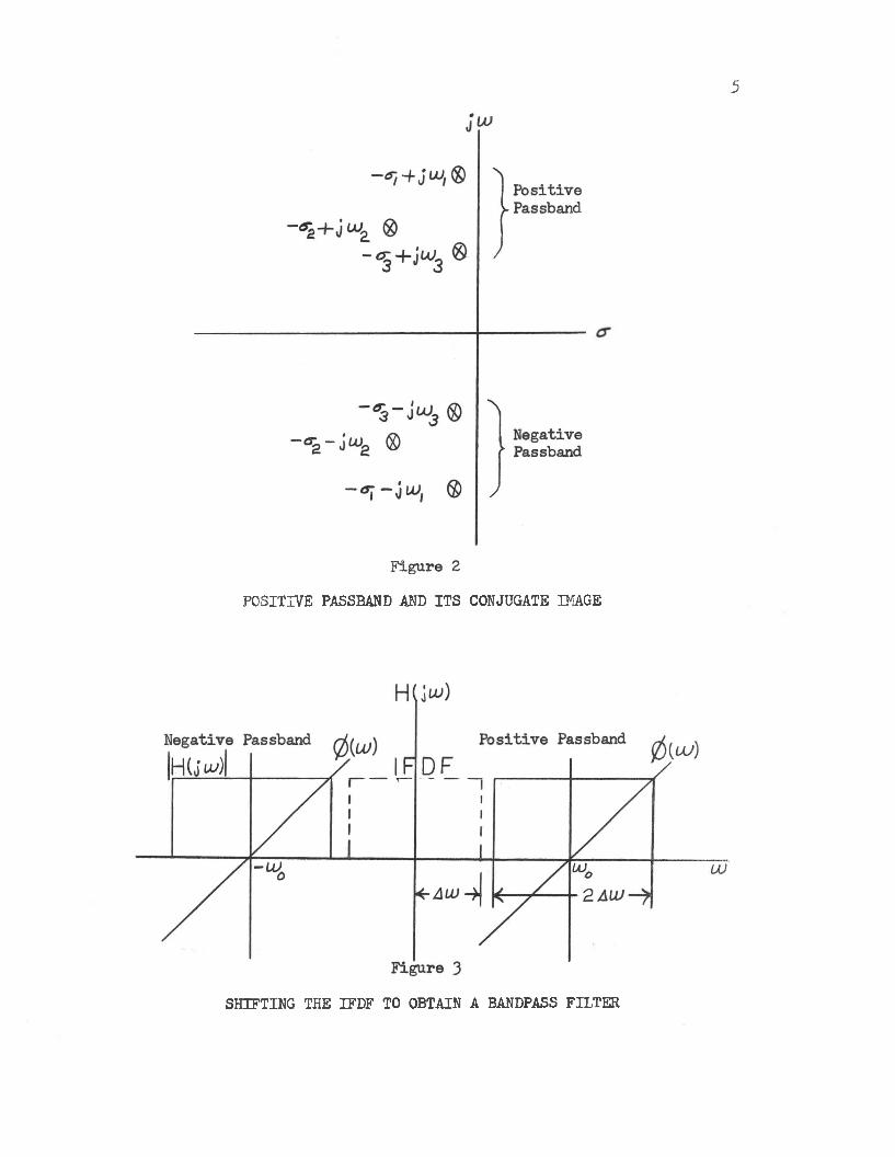
original pole location, frequency shifting the passband will yield a negative frequency passband. This is illustrated in Figure 2, Figure 3 illustrates the shifting of the magnitude characteristics to a new center frequency UJ0 with its corresponding image passband at Itshould be noted that the shifting of the low-pass prototype to a new center frequency doubles the bandwidth in the positive frequency range

as illustrated in Figure 3 (Ref. 3). Since the ideal bandpass filter can be realized only to within an approximation determined by the complexity of the realization.

5

POSITIVE PASSBAND AND ITS CONJUGATE IMAGE

SHIFTING THE IFDF TO OBTAIN A BANDPASS FILTER

CHAPTER III

APPROXIMATIONS TO THE IFDF AND IDEAL BANDPASS FILTER

I. LUTTERWORTH’S MAXIMALLI FEAT AMPLITUDE APPROXIMATION

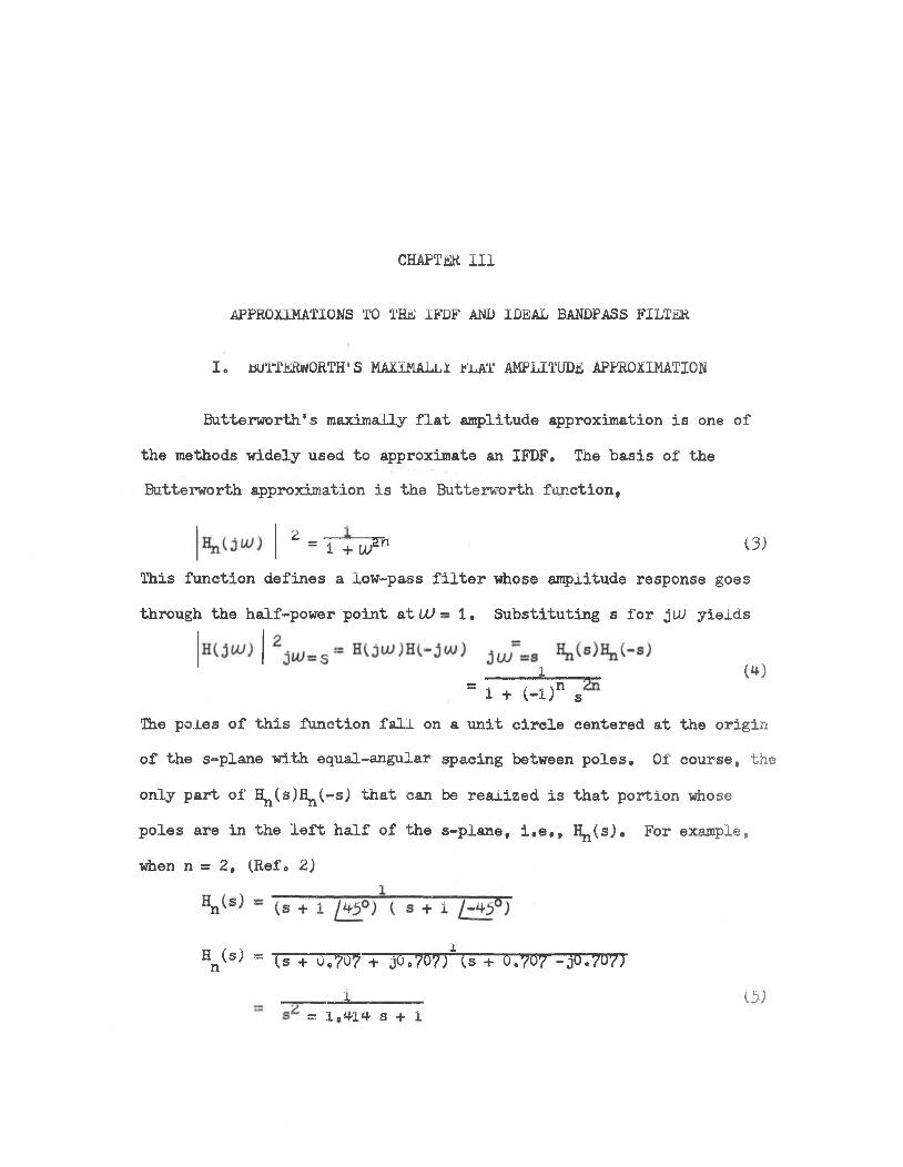
Butterworth’s maximally flat amplitude approximation is one of the methods widely used to approximate an IFDF, The basis of the Butterworth approximation is the Buttervorth function.

This function defines a low-pass filter whose ampxitude response goes through the half-power point at UJ - 1, Substituting s for jUJ yields

The poles of this function fall on a unit circle centered at the origin of the s-plane with equal-angular spacing between poles. Of course, the

only part of Hn(s)Hn (-s) that can be realized is that portion whose poles are in the left half of the s-plane, i.e., H^s), For example, when n = 2, (Ref. 2)

2 = 1 + u/n (3)

W1s 1 + C-l)n S

V s) = Is + o . w + jO.w/cs + 0.70? -"J0.7U7)I (5)

a 1,411 S + 1

7

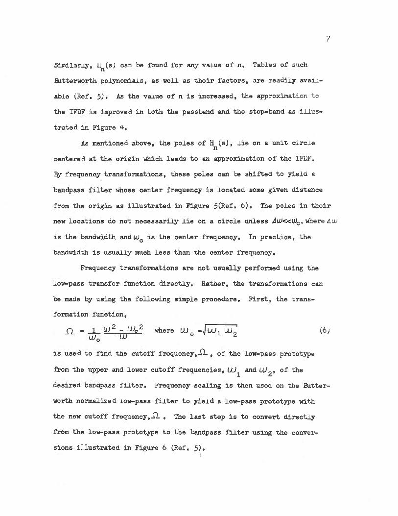
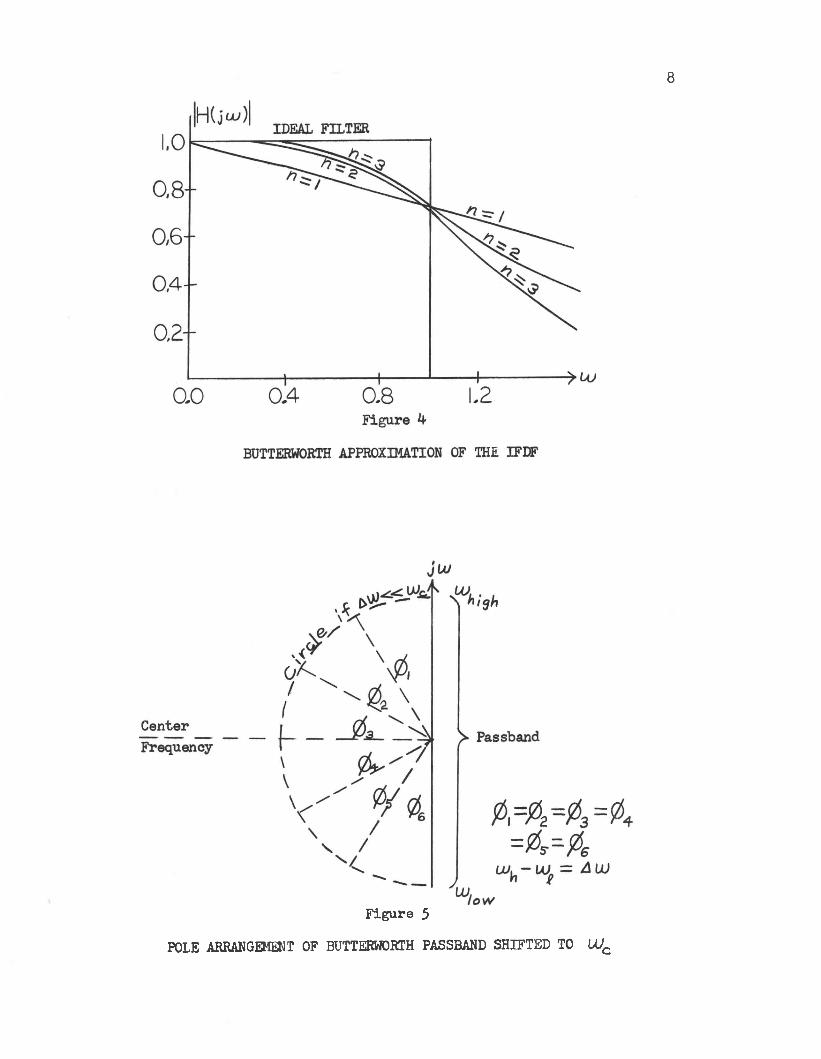
Similarly, Hn (sJ can be found for any value of n. Tables of such Butterworth polynomials, as well as their factors, are readily avail­able (Ref, 5)• As the value of n is increased, the approximation to the IFDF is improved in both the passband and the stop-band as illus­trated in Figure 4,

As mentioned above, the poles of H (s), lie on a unit circlencentered at the origin which leads to an approximation of the IFDF.Ey frequency transformations, these poles can be shifted to yield a

bandpass filter whose center frequency is located some given distance

from the origin as illustrated in Figure 5(Ref, b). The poles in their new locations do not necessarily lie on a circle unless All>«U)c, where Au) is the bandwidth and UJC is the center frequency. In practice, the bandwidth is usually much less than the center frequency.

Frequency transformations are not usually performed using the low-pass transfer function directly. Rather, the transformations can be made by using the following simple procedure. First, the trans­formation function,

X I = X tl>2 - M q2 where UU . =jbU1 UU ' (6)UJ0 LV c

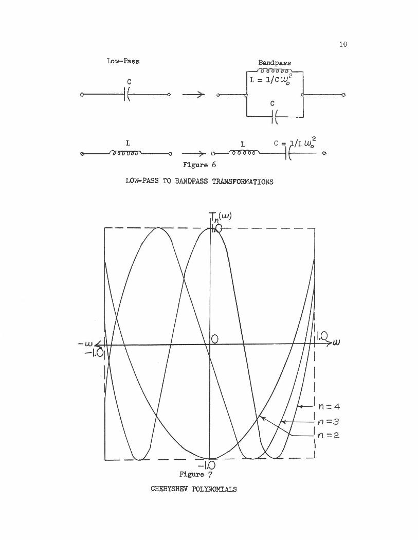
is used to find the cutoff frequency, XL , of the low-pass prototype from the upper and lower cutoff frequencies, UU and UU9, of the desired bandpass filter. Frequency scaling is then used on the Butter- worth normalized low-pass filter to yield a low-pass prototype with the new cutoff frequency,XI , The last step is to convert directly from the low-pass prototype to the bandpass filter using the conver­sions illustrated in Figure 6 (Ref, 5),

8

Figure 5POLE ARRANGEMENT OF BUTTERWORTH PASSBAND SHIFTED TO LUC

9

Some of the results of moving the poles about in the s-plane are:(Ref. 6)

1. As the poles are moved, away from the jtd-axis, the

amplitude over the entire range of real frequencies decreases;

2. the closer the poles are grouped together the narrower

the bandwidth of the resulting response;3. ana, as shown in Figure 5. maximum flatness is obtained

when the poles are spaced at equal-angular intervalsaround a circle if AUJ<c UJ ,c

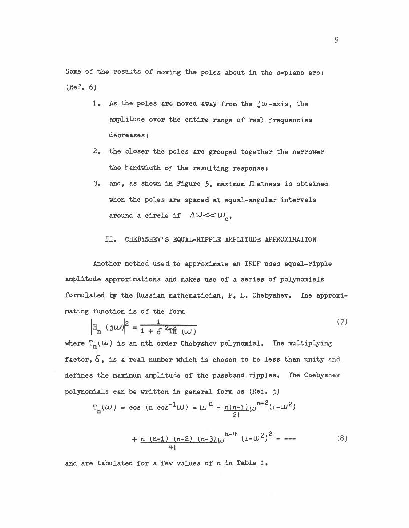
II. CHEBYSHEV'S EQUAL-RIPPLE AMPLITUDE APPROXIMATION

Another method used to approximate an IFDF uses equal-ripple amplitude approximations and makes use of a series of polynomials

formulated ty the Russian mathematician, P, L. Chebyshev, The approxi­mating function is of the form

where Tn (Ul) is an nth order Chebyshev polynomial. The multiplying

defines the maximum amplitude of the passband ripples. The Chebyshev

polynomials can be written in general, form as (Ref. 5)

(?)

factor, 8, is a real number which is chosen to be less than unity and

T (UJ) s= cos (n cos~^uJ) = UJ n - n(n-l) in 2(l-lU^)2!

+ n (n-1) (n-2) ( n ^ u/1"** U-tU2)2 (8)

and are tabulated for a few values of n in Table 1

Low-Pass

10

o- (---------°

Bandpass

L = 1/C UA2

L/inrzjTrcrtP- ■o

L----o— ' T n m mFigure 6

-o

LOW-PASS TO BANDPASS TRANSFORMATIONS

CHEBYSHEV POLYNOMIALS

11

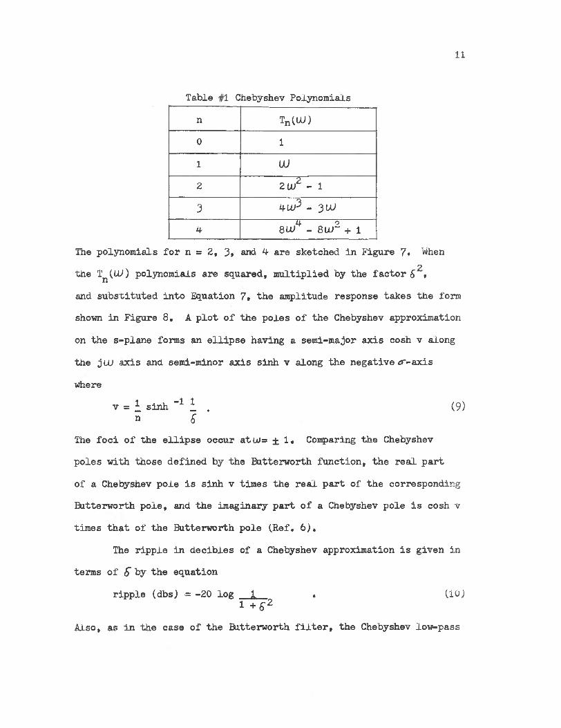
Table #1 Chebyshev Polynomialsn Tn(UJ)0 1i LU2 ZU)Z - 13 4uP - 3uu4

Zf o 8LU - 8or + 1

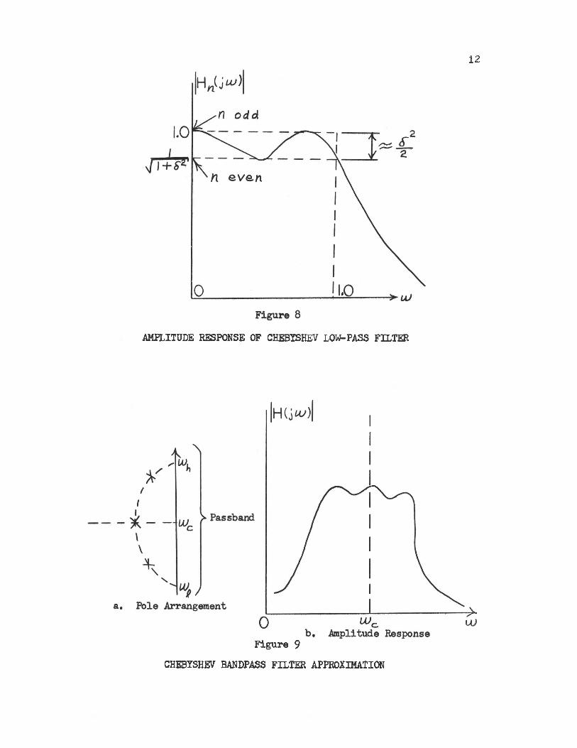
The polynomials for n = 2, 3* and 4 are sketched in Figure 7. WhenOthe Tn (llO polynomials are squared, multiplied by the factor £ ,

and substituted into Equation 7, the amplitude response takes the form shown in Figure 8. A plot of the poles of the Chebyshev approximation

on the s-plane forms an ellipse having a semi-major axis cosh v along the j UJ axis and semi-minor axis sinh v along the negative r-axis

where

v = £ sinh “*■ £ . (9)n 6

The foci of the ellipse occur atu/= ±1 . Comparing the Chebyshevpoles with those defined by the Butterworth function, the real partof a Chebyshev pole is sinh v times the real part of the correspondingButterworth pole, and the imaginary part of a Chebyshev pole is cosh v

times that of the Butterworth pole (Ref, 6),The ripple in decibles of a Chebyshev approximation is given in

terms of S by the equationripple (dbs) ■= -20 log 1 . (iOJ

1 + SZAlso, as in the case of the Butterworth filter, the Chebyshev low-pass

12

AMPLITUDE RESPONSE OF CHEBYSHEV LOW-PASS FILTER

Figure 9CHEBYSHEV BANDPASS FILTER APPROXIMATION

13

filter approximation can be frequency transformed to yield a bandpass

approximation. The grouping of the poles and a typical plot of ampli­tude response for the bandpass approximation are shown in Figure 9.

Once again, as in the Butterworth filter, the phase response will not be linear (Ref, 6),

III. MAXIMALLY FLAT DELAY APPROXIMATION

The two IFDF approximations discussed so far have been approxi­mations to the desired amplitude only. The phase response of these approximations was not intended to be very close to the ideal, since it was only a by-product of the desired amplitude response realization.

This being the case, this paper would not be complete without a dis­cussion of the maximally flat delay approximation.

The delay, or group delay function Tp, is the negative deriva­tive of the phase, 0 (UJ),

td = U DSince the desired phase is to be linear, the ideal time delay is a

constant. Assume that a voltage e^(t) having a Laplace Transform E^(s) is applied to a network. The desired output is a function of the form

e2(t) = e^t-Tp) where T^is a constant. But, ^ ^ ( t - T j ^ s e”sTD ^ ’ e1 (t) - or E2(s) = e"sTD Ej(s). Therefore, it can be seen that a network with a constant time delay must have a transfer ratio of the

form E2/E1 = e”sTD, If the ideal time delay, TD , is one second, then

this transfer ratio can be expressed asE2/Ei = H(s) = e~s = _______1_______

cosh s + sinh s(12)

This function is unrealizable with lumped components and must, there­

fore, be approximated.

14

It is known that

cosh s ss M(s) = 1 + ^ + 5— + ~ + -- (13&)21 41 6land

sinh s = N(s) = s + ^ 2 + I ^ + ^ Z + -- (13b)31 51 71

Rearranging Equation 12 gives

H(s) = 1 , ( Wsinh s (coth s + 1) bat coth s can be expanded into the infinite continued fraction

coth s = M(s) = 1 + _______ 1________________________________ .■N(s) s 3/s +________I_________________________

3/s + I___________________7/8 + — (13)

By truncating Equation 15 at the (2n - l)/s term, an nth order approxi­mation can be obtained. As an example, when n = 4, the expansion ends with 7/s and

M(s) = s4 + 45 s2 + 105N(s) i0s3 + 105 s , (16)

From Equations 12 and 13, it is seen that the denominator Bn (s) of

H(s) can be expressed as M(s) + N(s), For instance, when n = 4,Equation 16 can be used to find H^s) from the simple fact that

M(s) = s4 + 45 s + 105 = even funct,3 (17)

N(s) = 10 + 105 s = odd funct.Thus, the denominator of Hn(s) will be

Bn (s) = M(.s) + N(s) = s^ + 10s- + 45s + 105 s + 105 = %(s),(18)

The constant term of B^s) is usually placed in the numerator to adjust

15

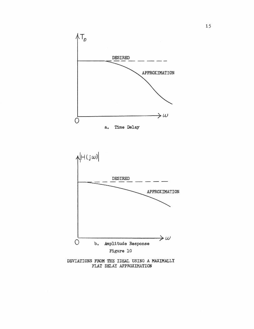
DEVIATIONS FROM THE IDEAL USING A MAXIMALLY FLAT DELAY APPROXIMATION

16

the amplitude response to unity for small values of s. The general form for approximating Equation 12 then becomes

H (s) = bo = _________________ . (19)n B^s) bQ + t^s + — + bnsnThe following general form for finding Bn (s) is useful for

determining the exact coefficient, of any particular power of s

(Ref. 6).B (s) = (2n - K)t sK for K = 0, 1, 1, — , n (20)

&=0 2n“K (n - K)J K!

Since Equation 19 is an approximation of Equation 12 about the origin, the desired response characteristics are cxosely approximated near UU = 0 with the accuracy decreasing at higher frequencies (Ref. 6). However, larger values of n produce approximations which are more accu™ rate at the higher frequencies than do those obtained using small val­ues of n. Figure 10 illustrates typical deviations from the ideal

obtained with this type of approximation. Tables of the coefficients and factors of B^s) can be obtained from any good book on network synthesis (see, for example, Ref0 5)•

The reader has probably already guessed that this approxima­tion was mainly intended to yield a phase response approaching the

ideal at the expense of the magnitude response. Thus, it should come as no great surprise that there is no sharp cutoff in the magni­

tude response when this approximation is used.

IV. DISADVANTAGES OF THESE APPROXIMATIONS

The methods discussed so far are among the most widely used

approximations to the IFDF and, yet, none of them approximate both

17

the ideal magnitude characteristic and phase response simultaneous­

ly. An all-pass section can be used to change the phase where desired without affecting the magnitude characteristics. "When a rectangular passband and linear phase shift are both necessary in a given applica­

tion, it has been customary to design the amplitude characteristic by the usual methods and then to equalize the delay with additional all-pass sections." (Ref. 4), This procedure is difficult to apply and increases the complexity of the filter.

The approximations which have been covered thus far tie the magnitude and phase characteristics together using a minimum phase

assumption (all zeros located in the left half plane). This assump­tion greatly simplifies the task of realizing such a filter, but it

makes it impossible to simultaneously realize an approximately rectan­gular amplitude and linear-phase bandpass filter characteristic (Ref. 4).

CHAPTER IV

LERNER'S BANDPASS FILTER APPROXIMATION

I. INFINITE NETWORK APPROXIMATION

Simultaneous approximation to both the ideal amplitude and

constant delay characteristics is possible by using a non-minimum phase design procedure discussed by Robert M, Lerner in his paper, "Band-Pass Filters with Linear Phase" (Ret, 1). His method will

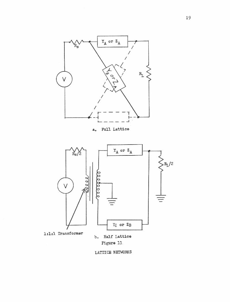
now be discussed,Lerner made use of the lattice network configuration in his

approximation. The full lattice configuration and its equivalent,

the half-lattice, are illustrated in Figure 11, To begin this dis­cussion, the voltage transfer function of the full lattice network is needed in terms of the arm impedances and admittances. It can

easily be shown that

V2 = G(s) = Rl _____________Zb^s) ~ 2a(s)______________ (21)Vs 2RsRj+CZbts)+Za(s)) (Rs+RL)+2Za(s)Zb (s) .

Similarly, the transfer function in terms of Y& and Yb is found to be

G(s) « ___________Ya ^ - V 5>>_________________2RgRLYa(s) Yb(s) + (Ya(s)+Yb(s))(Rs+RL) + 2

Assume each of the admittances Y& and Yb is initially comprised

of an infinite sum of individual poles, or resonances, spaced at equal

19

a. Full Lattice

lslsl Transformer b. Half Lattice Figure 11

LATTICE NETWORKS

20

intervals 4a units along a line b units to the left of the j UJ axis

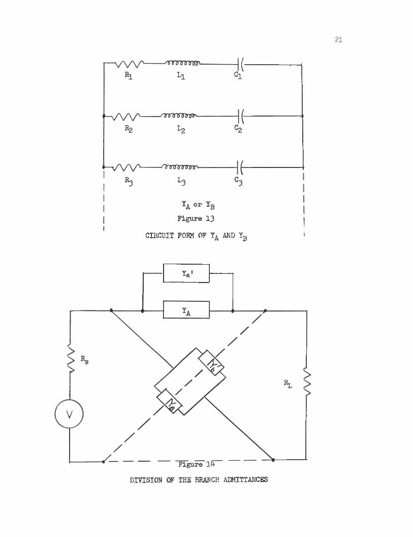
in the s-plane. Furthermore, let the poles of Y_ lie midway betweenclthose of Yb as illustrated in Figure 12, Thus, the circuit form of Ya

and Yb will be that of Figure 13. Assume also that P/ J RsRb is the residue at each pole, where P is a scale factor.

Using these assumptions, we obtain

y = > P/ n/R^RE (23) Yb = <T P/^ Rs^ (24)n Lccs + b - 4naj ^=1 s + b + 2aj - 4naj

These equations can be expressed in terms of hyperbolic functions as

Ya = 'tr b coth 'TT(s + b) (25)v/RsRl 4a

Yb = IT P tanh IT (s + b)7e ,»l 4a

(26)

CIRCUIT FORM OF YA AND Y3

V ?la

DIVISION OF THE BRANCH ADMITTANCES

22

Substituting the expressions for Y& and Y^ in Equation 22 we

obtain__________RL-TrP/4a_____________________

G(s) = pRsR^ (i + (TTP/^-a)^) Csinhtr(s + b)/2a)L +(Rs+Rl; (iTP/fa) (coshir(&+b;/2a;l (2?)

It is known that the sum of sinh u and cosh u is eu ; thus, by choosing TTP/ t-a to equalize the coefficients of the sinh and cosh terms in Equa­tion 27, G(s) can be made a simple delay operator. The resulting quadratic equation

[l + (TTP/4a)2] = (Rg + Rl) (TTP/^a) (28)has two solutions. They are

P Z / rTTl = ^ R L and 4a/TTRs . (29)Substituting either of these solutions in Equation 27 results in the

transfer functionG(s) = r2 (e“'rrb 2a Q-'TTs/Za , (30)

r s + r lby inspection, the infinite network which has been assumed

introduces a pure delay o,ftr/2a seconds and an attenuation of IT b/2a nepers in excess of that due to the source and load. Thus, there is no ripple in the attenuation or phase characteristics of the assumed net­

work,

II. TRUNCATION OF THE INFINITE NETWORK

Of course, it is not practical to realize an infinite network,

so some means of approximation must be used. First, however, consider the following well-known equivalence theorem for the symmetric lattice; "Any admittance Yq can be subtracted from each of the arms of a symmet­ric lattice and placed instead across both the input and output term­inals of the lattice without changing the terminal behavior of the

23

network," (Ref. 4), We must assume that the desired filter passband contains a modestly large number N of the consecutive resonances of

Ya and Y^. In addition, we will choose a nominal band edge halfway between the nearest in-band and out-of-band resonances, temporarily assume that N is odd, and assume that the first out-of-band resonances

belong to Y& at both ends of the passband. Since Ya and Yg consist of an infinite number of elements, they can be written as

Y = Y + I * a A + aYb - YB + V

where Y. and YD include all of the resonances of Y„ and Y, which lie A B a bwithin the desired passband, and Y&* and Y ' include the remaining

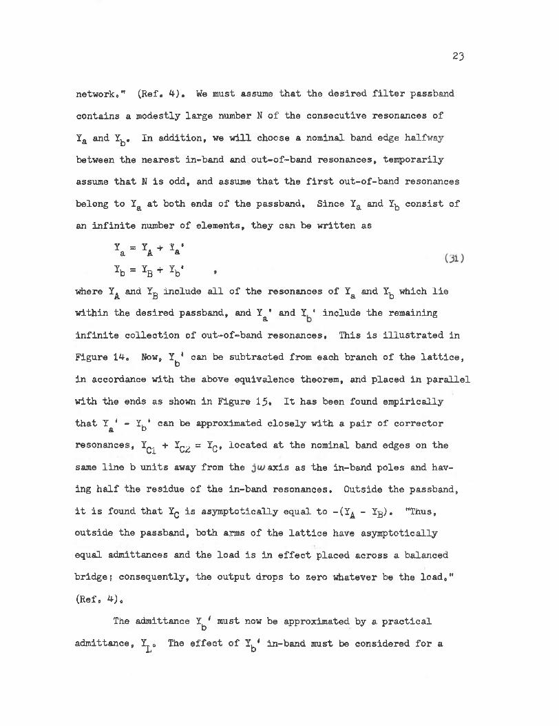
infinite collection of out-of-band resonances. This is illustrated inFigure 14. Now, Y * can be subtracted from each branch of the lattice,bin accordance with the above equivalence theorem, and placed in parallel

with the ends as shown in Figure 15. It has been found empirically that Ya" - Y-d‘ can be approximated closely with a pair of corrector

resonances, *C1 + rC2 - * C located at the nominal band edges on the same line b units away from the axis as the in-band poles and hav­ing half the residue of the in-band resonances. Outside the passband, it is found that Yq is asymptotically equal to -(Y^ - Yg). "Thus, outside the passband, both arms of the lattice have asymptotically equal admittances and the load is in effect placed across a balanced bridge? consequently, the output drops to zero whatever be the load,"

(Ref. 4),The admittance Y^/ must now be approximated by a. practical

admittance, Y^0 The effect of Y ^ in-band must be considered for a

24

u

Figure 15 - Transformation of Lattice

25

good approximation. This admittance consists of the sum of resonances

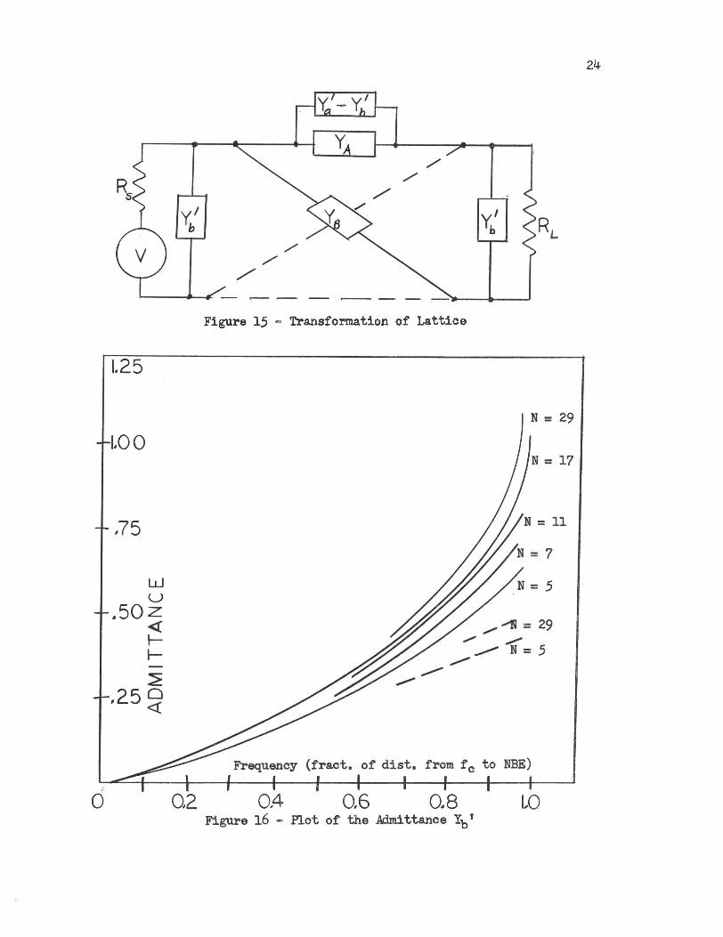
placed every 4a units outside the nominal band edge, starting with a position 3a beyond the band edge and can be expressed in closed form SLS

Xh (32),___. in (§±b + 3 )- W (2Nt2 “ 3±bv4jajRsRjj [J 4ja 4 r 4 4ja_lwhere (p (Z) = d/dz (log | (z)', If P is assumed to be that foundin Equation 29, and if we assume that b « a (components are very close

to being lossless), then Equation 32 reduces to

Yb = _iTTjE

in (_A_ + J) " UJ (2Rf3 " A) r K 4a v r 4 4a

(33)

This admittance is plotted in Figure 16„ As can be seen from the fig­ure, the admittance is zero at the band center and is very nearly a linear function of frequency except in the vicinity of the band edge.

Since a parallel LC circuit exhibits a reactive admittance which is zero at the band center and varies nearly linearly with frequency, it can be used as an approximation. Thus, Y^* can be replaced by an LC

parallel circuit having the same slope at the band center as Y '.bThis means that the LC circuit must have a loaded Q of

«L - * * V 4 f 1 Wwhere Af/f is the fractional bandwidth of the filter and k„ varies o Nfrom 3/5 for modest N to 2/nr for large N,

Having found approximations for all assumed infinite network

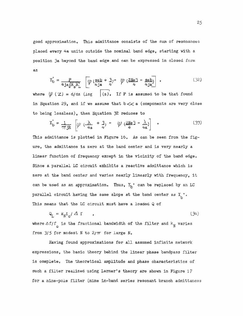
expressions, the basic theory behind the linear phase bandpass filter is complete. The theoretical amplitude and phase characteristics of such a filter realized using Lerner“s theory are shown in Figure 17

for a nine-pole filter (nine in-band series resonant branch admittances

26

•“ >■Ll <X — 1 LO LlJ Q

Figure 1?

NIKE”POLE FILTER

27

plus two corrector resonances on the Input and output of the network).

These characteristics are those of a bandpass filter in the 15-20 KC region. As can be seen from this figure, the top of the amplitude

characteristic is very flat and the phase is practically linear over the 15-20 KC region. According to Lemer, the cutoff of the amplitude characteristic as well as the linearity of the phase can be improved

by adding more in-band resonances or by inserting more zeros in this stop-band by bridging across the source and/or load series resonant

circuits which have roughly the same admittance level as the network branches in-band. Thus, if Lemer's theory can be used to realize

filters which have the magnitude and phase characteristics that he predicted, it has several advantages over the previously discussed

methods.

CHAPTER V

REALIZATION AND ANALYSIS OF LERNER'S

BANDPASS FILTER APPROXIMATION

I. METHOD OF REALIZATION

The realization of a filter using Lemer's theory is largely accomplished using only Equations 23 and 24 in conjunction with the truncation steps introduced following the discussion of these equa­

tions, Of course, the desired bandpass must be specified and the pole pattern in the s-plane determined as discussed earlier. The residue

P / V ® 1^2 is determined using Equation 29. After the truncation steps are made. Equations 23 and 24 contain only in-band poles or resonances and are easy to realize. The realization steps for YA follow.

Realization of Y . Referring to Equations 23 and 24, letting P/jB R ~ A, where A = constant, and 4naj = Bnj, we have

Y _ ...A .1, 4 I, A 4* AXA “ 8 + b - Bn^j s + b + Bn^j s + b - Bn^j

+ A + — (35)s + b + Bn2j

The number of terms above will be twice the number of J& in-band poles(must include the conjugate of each term). Therefore

Y, = J A L&jt b)---- + 2A (s j Dj___ + —A (s + b)2 + (Bn^)^ (s + b)^ +

(36)

The above equation can be put in realizable form by dividing by

2a(s>+ b). Thus,

+

29

Y = _____________ 1A (1/2A) (s + b) + 1 _________(2A/Bn1)0 (s + b)

07)

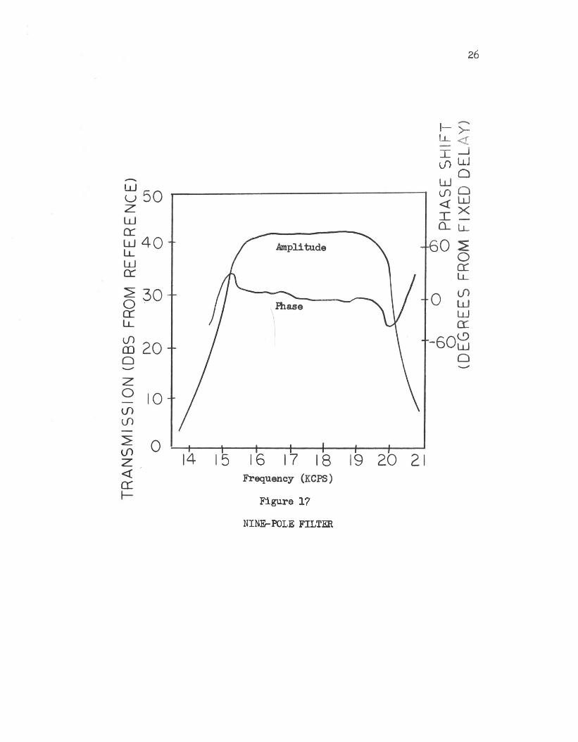
The second term was omitted in the preceding equation, since the procedure is the same for both terms. The component values are easily-

taken from the equation in this form. Indeed, the circuit form is that

of Figure 18.

R1 L1 if----- M w ------nnnnr'— <> <>-----------

><------------------ — --------------=>©

Hf-cir2

AA/\A

Figure 18

CIRCUIT FORM OF THE INDIVIDUAL ARM RESONANCES

The values of the components are obtained from the following equations*R1 s b/2A (ohms) (38a)

m 1/2A (henrys) (38b)R2 ** (Bn^) ^/2Ab (ohms) (38c)C1 = ZA/iBn.^ (farads) (38d)

From the above equations, it can be seen that the inductance and R^

are the same for all the shunt branches of YA’ but the capacitance and R2 change in each case. The in-band resonances of Y are realizedDin the same manner. The component values for Xg resonances are given

by

30

R1 = b/2A (ohms) (39a)

L1 = 1/2A (henrys) (39 b)

r2 = (2a-4n1a)2/2Ab (ohms) (39c)

C1 = 2A/(2a-4n1a)2 (farads) (39d)

Comparing the above equations to those in Equations 38, and are identical to R^ and in Y^. Also, (Br )2 in Equations 38 is merely the radian frequency location squared of each IA pole, and (2a-4na)2 in Equations 39 is merely the radian frequency location squared of each Yg pole. Finally, the resistances, R^ ana R^, can

be completely neglected if b « a (components close to being lossless) yielding a simple LC series resonant circuit. These observations make it very easy to realize the YA and Yg resonances, as will, be shown

later in a sample realization.

The pair of corrector resonances, YC1 and YC2’ placed in shunt with Y^ when N is odd and the first across Y^ with the second across

Yg when N is even, have the same form as Y^ and Yg and are realizedby the same technique. This leaves nothing but Y to be realized,.LThis, however, is simply a parallel LC circuit resonant at the center

frequency of the bandpass and having the Q specified in Equation y+.

The following is a seventh order (N = 7) sample realization using the above-derived realization techniques,.

Seventh Order Leraer Realization.

Specifications;1, 7 in-band poles.2, 1,0 X 106 rps, = LUQ — band center.3, % bandwidth

31

4, bc<a.5 . Rg = Rg = 1 .0 ohm.

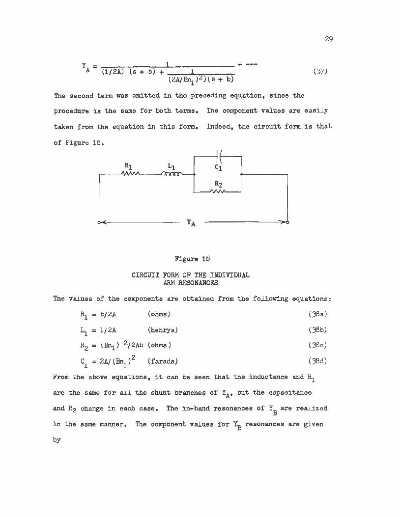
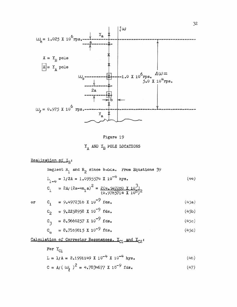
The pole locations of YA and Yg are sketched in Figure 19. Neglec­ting b, the pole locations in Figure 19 are found to be

s = j l . 0214286 X 106 ------------ Yfi

s = jl.0142857 X 106 Yas = j l , 0071428 X 106 Yg

s = j l . 0000000 X 106 -------------ya

s = jO. 9928571 X 106 ------- Ygs = jO.9857143 X 106 Yas = jO .9785714 X 106 ------------ YB

2a = (5.0 X 104)/7.0 = 7.1428571 X 103a = 3.5714285 X 103 (40)

The residue. A, is found from Equation 29 to be

A = 4a/rrRs = 4aAn-RL = 4.5472840 X 103 . (41)The components in YA will be found first.Realization of %Ai

Neglect R^ and Rg since b « a . From Equations 38

l1-3 = 1/2A = 1.0995574 X 10“^ hys.Ci = 2A/(Bn1)2 = 2(4.5472840 X 103)

(0.9857143 X 108)2

(42)

or Cx = 9.3600894 X 10”9 fds.c2 = 2(4.5472840 X lo3)/(l,000 X 106)2

(43a)

or C2 = 9.0945680 X 10~9 fds. (43b)

C3 = 8.8401873 x 10~9 fds. (43c)

32

Figure 19 ya and yb POLE LOCATIONS

Realization of Y-tNeglect R^ and R^ since b<Ka. From Equations 39L. /( = 1/2A = 1.0995574 X 10”4 hys. (W)l-*+C1 = 2A/(2a~4n a)2 = 2(4.547280 X 10^)_

(0.9783714 X 10°)^or C± = 9.4972316 X 10"9 Ids, (45a)

C2 = 9.2238958 X 10~9 fds. (45b)

C3 = 8.9660257 X 10~9 fds. (45c)= 8.7169815 X 10“9 fds. (43d)

Calculation of Corrector Resonances. Y^ and -IC2‘For YC1L = 1/A = 2.19911^9 X 10“4 X 10"4 hys. (46)

C = A/( )2 = 4.7834677 X 10~9 fds. (47)

33

8.8401873 X 10"9fd.t------ smrsvv 1.9.O&568O X 100995574 X 30"4 hy. 0-9fd.

-/dfrboot | >

1.0Ohm

41 ■ ' ii i m *lv 1.0995574 X OjO" hy.

9.3^00894 X 10-9 fd .I------ M Un r

— / T O W ------1 - . »0995574 X no-4* hy, i 4.7 34667 X lC-9fd. ,

l( 2.19911 9SV l 0 “4 hy.' 4.3 81704 X 10’9fd. I

|{~Xl991lWVlO-4 hy.I

9.4972316 X 10"9fd. I

\9.2 258— rtnnnr\— , 0995574 x 30-% l0“9fd.— npnsm— j ,/ 0995574 x_8.3333&33£L0

1.2®)"-5fd.

I

l

1

8.19660257 X 10-9fd.\L------<Tnram__IV 1.0995574 xlfo

8.|7l69§15 X 10“9fd,6 tt'OITv.—1J,0995574 x 10

Figure 20LERNER SEVENTH ORDER FILTER NETWORK

34

and, similarly, for Y ^

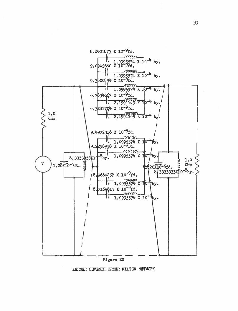
L = 1/A = 2,1991149 X 10-4 hys. (48)C = A/( U3h)2 = 4.3281704 X lO-9 fds, (49)

Calculation of Y^‘ or Y^ 1 1

Begin by finding the loaded Q and the L and C relationships,= kN UJ0/ALU = (3/5) (1.0 X 106)/ (5.0 X 104) (30a)

or Ql = 12,00 (50b)UJ CR = Q (51)o LR/ UJ QL = Ql (5k)R = = Rg = 1,00 ohmC = 12.00/1.0 X 106 = 1,2000 X 10"5 fds. (53)L = 1.0/1.2 X 107 = 8.3333333 X 10”8 hys. (54)

This completes the realization. The complete circuit is that of Figure

20.

II. ANALYSIS OF REALIZED LERNER FILTERS

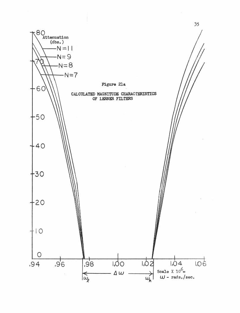
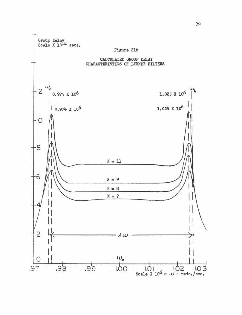
Lemer Filters of Orders 7. 8. 9. and 11. Lemer filters with N = 7. 8, 9, and 11, a 5$ bandwidth, center frequency of 1.0 X 108 rads/sec., and b « a were realized using the procedure just described. These realiza­tions were analyzed using the computer program CXTLTC, written by Humpherys (Ref, 3). The magnitude and group delay characteristics are plotted in Figures 21a and b respectively.

35

36

37

Referring to Figure 21a, it is evident that the cutoff rate

and the out-of-band attenuation increase with the order of the filter. This is due to the increasing number of resonances near the band edges. Supporting Lemer's claim that practically zero magnitude ripple is

obtained in the passband if the residue is calculated as was done in Equation 41 in the sample realization, the passband ripple was very small using this residue (of the order of 0,002 dbs, for N = 7 and

less for N > 7) (Ref, 40,Referring to Figure 21b, there were bumps in the group delay

characteristics at 0,974 X 10^ rads/ sec, and 1,024 X 10^ rads/ sec, (very near the band edges). The magnitude of these bumps increased

with increasing N, suggesting a relationship between the cutoff rate and the magnitude of the group delay bumps (this will be discussed in

a later chapter). For example, the group delay bumps for N = 7 were of the order of 6,46 X 10“^ secs, while those for N = 11 were 10,42 X 10"^ secs. These bumps were located 2$ of the bandwidth from the

band edges for all values of N, The group delay was essentially con­stant over 72$ of the bandwidth for N = 7, 76$ for N = 8, 80$ forN = 9, and 84$ for N = 11, Thus, the percentage of the band over which

the phase is linear can be increased by increasing the order of the filter. The greatest group delay ripple in the passband was obtained with N = 11 and was of the order of 2,75$ (excluding the group delay

bumps near the band edges). The ripple for N * 7 was 1,58$, 1.79$ for N = 8, and 2,12$ for N = 9. Thus, the group delay ripple percen­tage increased slightly with increasing N. This can easily be seenfrom Figure 21b, The values used to calculate the above percentages

38

were obtained using the lowest value of the group delay in the small dip near the group delay bumps (most pronounced for N = 11) and the highest value of the group delay located near the band center. The

major reason for the small dip in the group delay, which accounts for

the ripple percentages calculated above, is the uncompensated curva­ture in the Y ' characteristics near the nominal band edge (see Figure

16). As N increases, the curvature of the Y, 1 characteristic increases near the band edge making the parallel LC circuit, Y , farther from the

Xj

desired Y^* characteristic in this region. This causes the dip in the group delay characteristics to increase slightly as N increases. Possi­bly, the addition of shunt resonances just outside the passband, so as to better approximate Y^', would improve the linearity of the group

delay curve.Effects on Lemer's Approximation of Increasing the Bandwidth

The effect on the magnitude and group delay characteristics

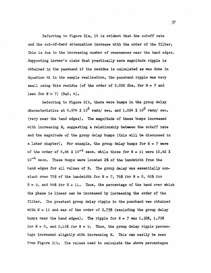
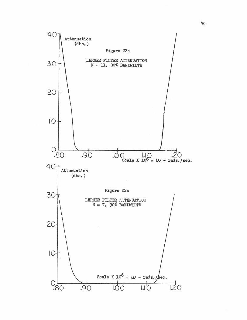
of increasing the bandwidth from % to was the next thing which was investigated. Two Lemer filters with such a bandwidth were real­ized, one with N = 7 and one with N = 11. None of the other character­

istics, band center, etc. were changed. Once again, the magnitude and

group delay characteristics were found using the computer program CXtLTC. These characteristics are plotted in Figures 22a and b.

39

Referring to Figure 22a, the only evident differences between

the magnitude characteristics obtained with a % bandwidth and those with a 30% bandwidth were a slight lack of symmetry and a small increase in the in-band ripple (0,02 dbs, as compared to 0,002 dbs,) with a 30# band. The rate of cutoff was greater on the high frequency side of the band than on the low frequency end. However, this effect was expect­ed with an increase in the bandwidth from previous experience with bandpass filters. The slight increase in the in-band ripple was

probably due to the greater spacing between poles with the larger passband, and a lack of geometric symmetry of the poles about the band center.

As can be seen from Figure 22b, the group delay was also unsym- metrical. The peak at the high end of the band was greater than the peak at the low end (once again, this suggests a relationship between

the cutoff rate and the change in the group delay which will be dis­cussed later). The constant values of the group delay were lower with the greater bandwidth, but there was little or no change in the percen­

tage change of the group delay at the bumps on each end of the band from that obtained with a 5% band.

The effects on Lemer's filters of introducing inductor errors, resonant frequency errors, load and source resistance errors, and lossy

coils will now be discussed.Effects of Inductance Errors.

A ±10% inductance error was introduced in each coil of two Lemer

filter realizations with N = 7 and N = 9. All of the other filter specifications were kept the same as in the previous examples. Every

40

41

Delay 10"5 secs.

Figure 22bLERNER FILTER GROUP DELAY

N a 11, 30# BAND

,90 11 00 l / o 1.20Scale X 10b = UU - rads./

42

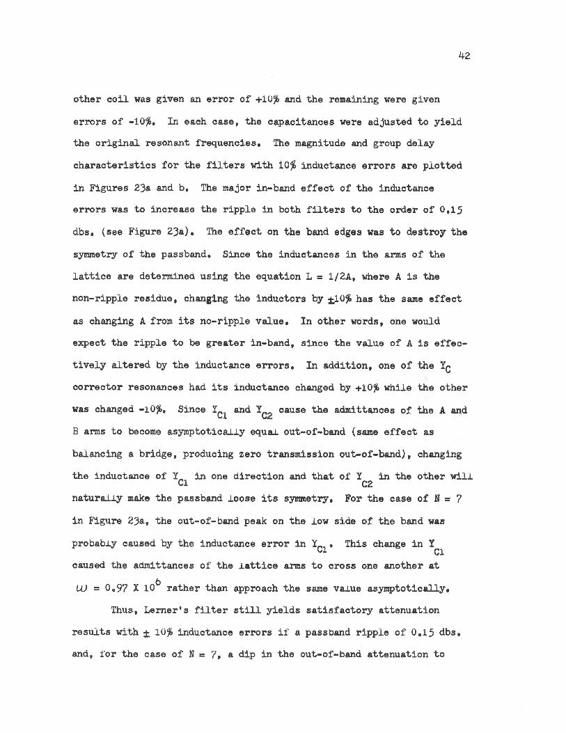
other coil was given an error of +10$ and the remaining were given errors of -10$, In each case, the capacitances were adjusted to yield the original resonant frequencies. The magnitude and group delay

characteristics for the filters with 10$ inductance errors are plotted in Figures 23a and b. The major in-band effect of the inductance errors was to increase the ripple in both filters to the order of 0,15 dbs, (see Figure 23a), The effect on the band edges was to destroy the

symmetry of the passband. Since the inductances in the arms of the lattice are determined using the equation L = 1/2A, where A is the non-ripple residue, changing the inductors by ±10$ has the same effect as changing A from its no-ripple value. In other words, one would expect the ripple to be greater in-band, since the value of A is effec­

tively altered by the inductance errors. In addition, one of the Yq corrector resonances had its inductance changed by +10$ while the other was changed -10$, Since Y^ and Y^ cause the admittances of the A and B arms to become asymptotically equal out-of-band (same effect as

balancing a bridge, producing zero transmission out-of-band), changingthe inductance of Y„ in one direction and that of Y in the other willCl C2naturally make the passband loose its symmetry. For the ease of N s 7

in Figure 23a, the out-of-band peak on the low side of the band was

probably caused by the inductance error in Y__ , This change in YCl Clcaused the admittances of the lattice arms to cross one another at

UJ = 0,97 X 106 rather than approach the same value asymptotically. Thus, Lerner's filter still yields satisfactory attenuation

results with ± 10$ inductance errors if a passband ripple of 0,15 dbs, and, for the case of N = 7, a dip in the out-of-band attenuation to

43

Group Delay Scale X 10“^ secs.

-14.0

- 12.0

Figure 23b

LERNER FILTER GROUP DELAY N = 7 AND 9, 10# L ERRORS

45

30 dbs. are permissible, In a practical application, the dip in the

out-of-band attenuation for N = 7 could be removed by juggling the inductance value in Y^.

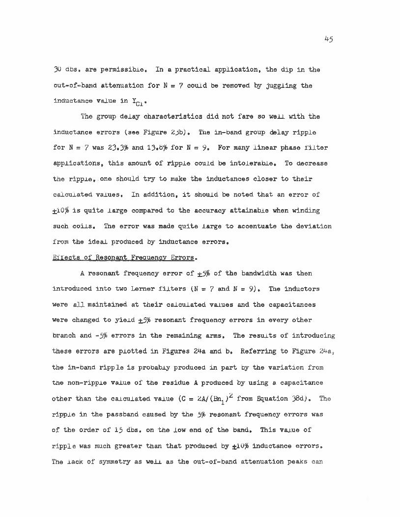
The group delay characteristics did not fare so well with the inductance errors (see Figure 23b). The in-band group delay ripple for N = 7 was 23.3% and 13.b% for N = 9. For many linear phase filter applications, this amount of ripple could be intolerable. To decrease tne ripple, one should try to make the inductances closer to their calculated values. In addition, it should be noted that an error of ±10% is quite large compared to the accuracy attainable when winding such coils. The error was made quite large to accentuate the deviation from the ideal produced by inductance errors.Effects of Resonant Frequency Errors.

A resonant frequency error of ±5% of the bandwidth was then introduced into two Lerner filters (N = 7 and N = 9 ). The inductors

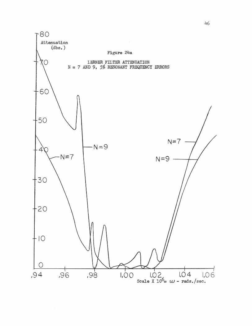
were all maintained at their calculated values and the capacitances were changed to yield ±5% resonant frequency errors in every other branch and -5% errors in the remaining arms. The results of introducing these errors are plotted in Figures 24a and b. Referring to Figure 24a,

the in-band ripple is probably produced in part oy the variation from tne non-ripple value of the residue A produced by using a. capacitance

other than the calculated value (C = 2A/(Bn^)^ from Equation 38d), The ripple in the passband caused by the 5% resonant frequency errors was of the order of 15 dbs. on the low end of the band. This value of

ripple was much greater than that produced by ±10% inductance errors.The lack of symmetry as well as the out-of-band attenuation peaks can

46

,94 ,96 ,98

47

48

be attributed, to the same causes described in connection with the introduction of inductance errors. There is one feature which is unique, however, in the case of resonant frequency errors. This fea­ture is the error in the location and width of the passband, especially

for N = ?• For the simple reason that the resonant frequencies deter­mine the pole locations and the pole locations determine the passband,

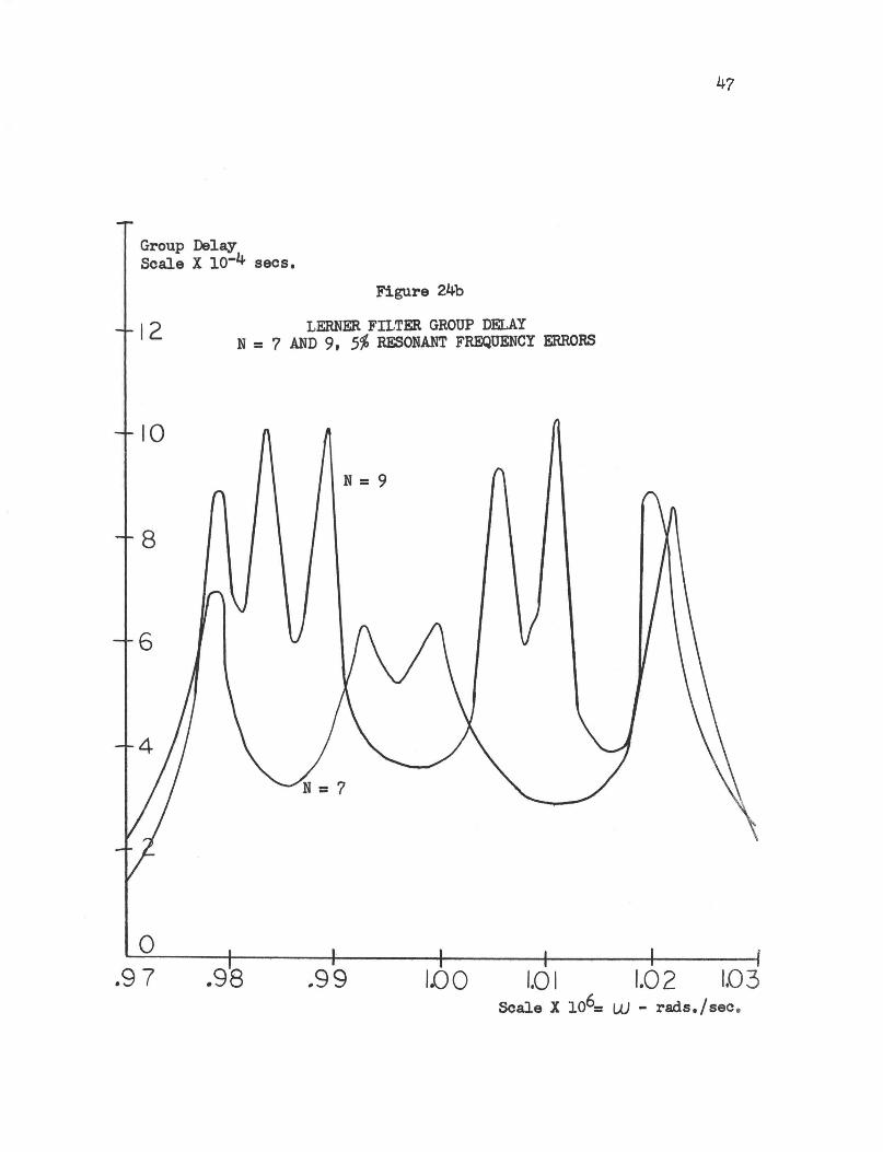
this is to be expected. Since the passband was so badly mutilated by the resonant frequency errors, uhe exact, error in band location and width will not be discussed. The group delay plots in Figure 24b

indicate that the ±5% resonant frequency errors adversely affected tne linear phase characteristics, too. In fact, the phase could hardly be

sailed linear any more. The in-band group delay ripple was as high as 100$ of the average value. These errors, produced by errors in the resonant frequencies, need no further discussion except to say that one must keep the deviations from the calculated resonant frequencies

as small as possible, since they are so critical in determining the magnitude and phase passband characteristics.

Effects of Varying the Load and Source Resistances.Variations of the load and souroe resistances from the vaxues

used in realizing a Lemer filter will now be discussed (Ref, 4), The load and source resistances of a seventh order Lemer filter were given an error of % and then an error of 10% and the effects on the magnitude and phase characteristics observed. The effects on the filter charac­teristics were very small. The primary effect was a slight increase in the passband magnitude ripple from 0.002 dbs, to 0,02 dbs. with a 10% resistance error. The change in the group delay was negligible.

49

These results tend to verify Lemer's assertion that a modest percen­tage of load ana source impedance errors should result in periodic errors which are of the second order in small quantities. Furthermore, according to Lemer, this is true even if the discrepancy is complex in nature (Ref, 4),Effects of Using Lossy Coils.

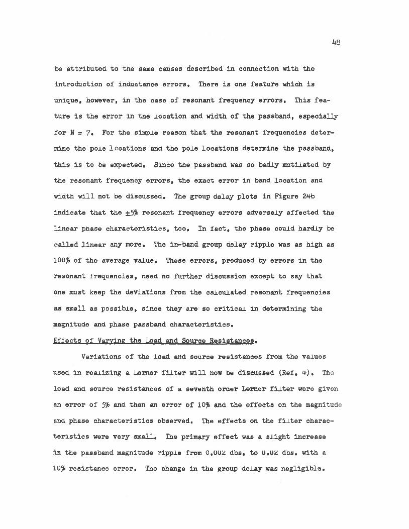
The introduction of lossy coils into a Lemer filter will be the next topic of this discussion. The coils were maae more lossy than would be the case in a practical application to accentuate the effects of a finite coil Q on the filter characteristics. A resistance

of one ohm was inserted in series with each coil in a seventh order filter to obtain the effects on the filter characteristics produceh by

lossy coils. This value of resistance in series with each coil yielded

an average Q of H O at UU a 1,0 X 10^ rps. The results are plotted in

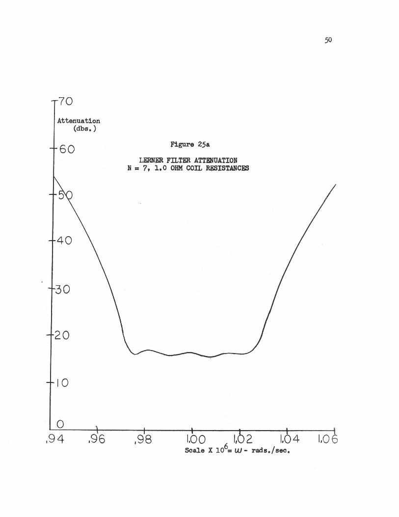
Figures 25a and b„ Referring to Figure 25a, the rate of cutoff decreased by 57% from that obtained with an infinite Q in Figure 21a,

Following the previously observed trend, the group delay bumps were smaller corresponding to the decreased rate of cutoff. The in-band attenuation increased to an average of 16 dbs,, and the out-of-band attenuation decreased. These results were expected from previous experience with finite Q‘s in other types of filters. The passband still retained its former symmetry and location. The two disturbing

results of a finite Q on the filter characteristics were an increase in the in-band magnitude ripple and some loss of phase linearity (see Figure 23b), After some careful study, it was found that the

corrector resonance, 1^, caused the increase in ripple. The effect

50

,98

51

,97 ,98 ,99

52of the corrector Y^, according to Lerner (verified later in this paper),

is to decrease the passband ripple in both the group delay and the mag­nitude characteristics. Recalling the method of realization of Y^, this corrector depends heavily on the value of its Q for its smoothing action in the passband. When a 1,0 ohm resistance was inserted in series with the coil in Y^, the value of its Q was no longer that used in calculating its components. This resulted in an increased passband

ripple. Thus, in a practical application, the Q of the coil Y^ must always be considered when calculating the values of L and C in this corrector. In addition, the finite Q's of the series resonant circuits,

in a practical application, should be taken into consideration when designing such a filter by using a finite value of b (distance from the juJ axis to the poles).

The effects of omitting corrector resonances and the insertion of out-of-band zeros make up the final topics of discussion concerning Lerner's filters.

Effects of Omitting the Corrector Y^.Two Lerner filters, one with N = 9 and one with N s 11, were

realized and the corrector Y^ omitted. The results are not plotted, since omitting Y^ simply increased the magnitude and group delay

ripple in the passband. For N = 9» the passband ripple was of the order of 0,77 dbs, and 1,0 dbs. for N a 11, The ripple values with Y^

included were 0,001 dbs, for N = 9 and 0,02 dbs, for N = 11, The group delay ripple with no Y^ was 9»2# for N = 9 and 12,1# for N = 11 as com­pared to 2,12# for N s 9 and 2,75# for N s 11 for Y^ included. These

results verify Lerner's claim that the effect of Y^ is to decrease the passband ripple (Ref. 4),

53

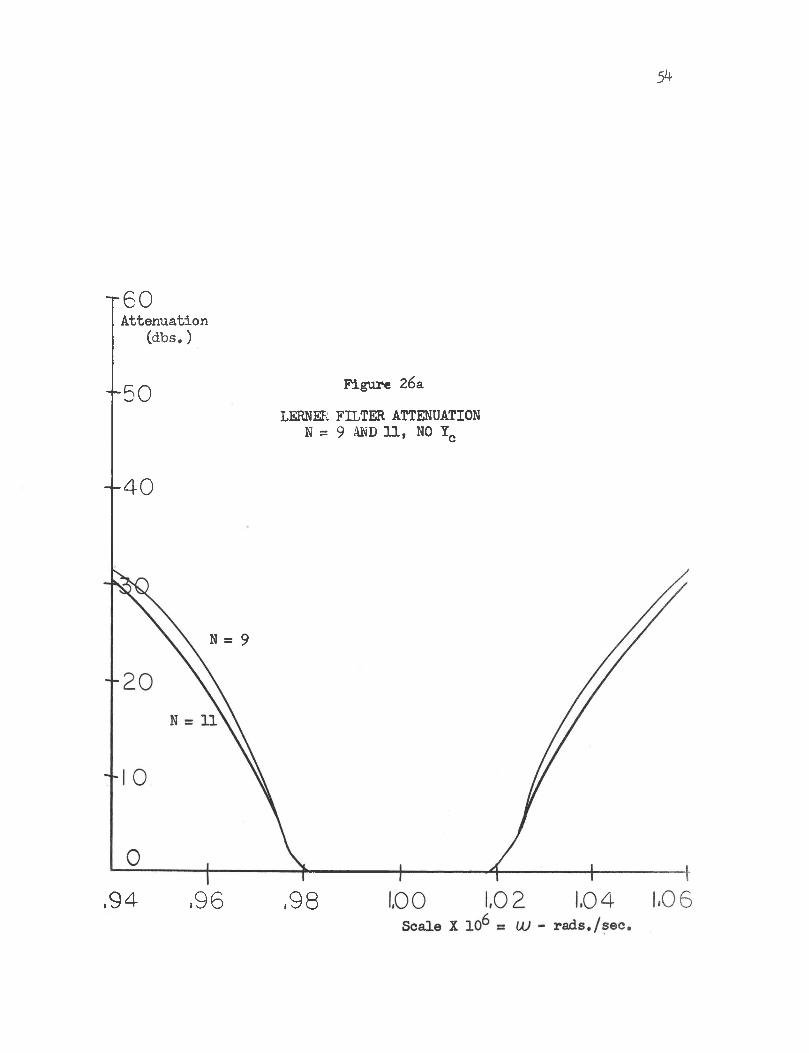
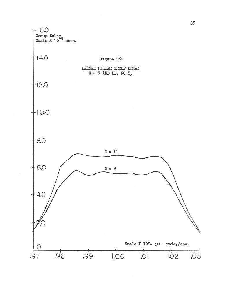
Effects ol' Omitting the Correctors and Y ^ .

Two other Lemer filters, one with N = 9 and one with K s 11, were realized and the correctors Yc omitted. The results of this omission are plotted in Figures 2ba and b. Referring to Figure 2ba,

the rate of cutoff and the out-of-band attenuation decreased as a result of omitting Y^. This was expected, since one of the purposes of the Yc correctors is to cause the A and B arm admittances to approach one another asymptotically and effectively place the load across a

balanced bridge out-of-band (Ref, 4), Other than this, there was no significant change in the magnitude characteristics. Once again,

corresponding to the decrease in the rate of cutoff, the group delay bumps decreased in magnitude. In addition to this result, the in-Dand

group delay ripple increased (see Figure 2bb) due to the lack of compensation at the two band edges,

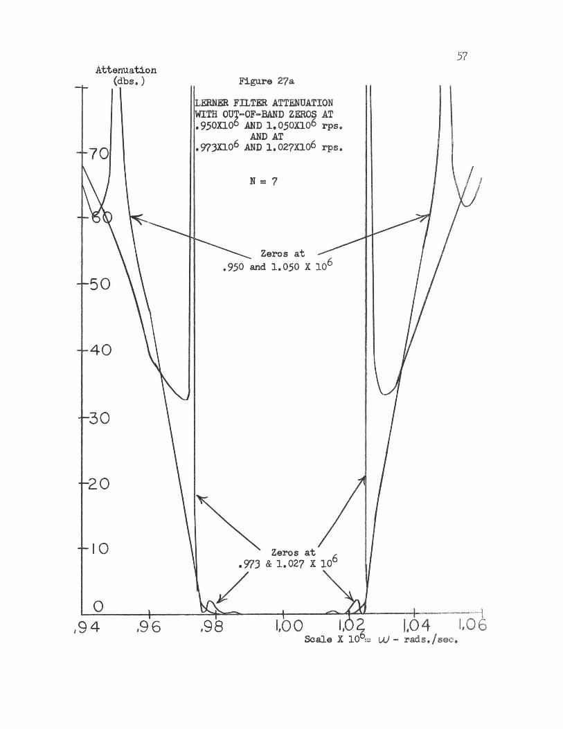
Effects of Adding Qut-of-Band Zeros.According to Lemer, after a given network design (realized

using Lemer*s theory) is complete, one can insert zeros in the stop- band, if desired, by bridging across the source and/or load series resonant circuits which have the same value of inductance as the series

resonant circuits in the A and B arms. Furthermore, Lemer claims,"The insertion of a transmission zero in this fashion results in no significant degradation of the attenuation elsewhere in the filter

stop-band, and tends to improve the approximation to a constant gain and delay within tne passband." (Ref, 4). Two Lemer filters with N = 7 were realized to check this claim, one with stop-band zeros at

0,9^0 X 10b and 1,030 X 10b rps, and the other with zeros at 0,973 X

5^

t 60Attenuation

(dbs.)

-50 Figure 26aLERNER. FILTER ATTENUATION

N = 9 AND 11, NO Yc

-40

N = 9

,94 ,96 ,98

55

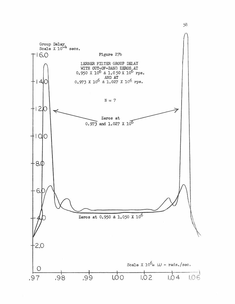
A 6 5610° and 1.02? X 10 rps. The results are plotted in Figures 27a and b.

Referring to Figure 21a and its accompanying discussion, the passbandripple with no stop-band zeros was 0,002 dbs. The addition of stop-bandzeros at 0,950 X 10^ and 1.050 X 10^ resulted in an increase to 0.01dbs. ripple in the passband. Stop-band zeros at 0.973 X 10^ and 1.027

X 10^ rps. increased the passband ripple to 2.4 dbs. (see Figure 27a).Following the trend of the magnitude characteristics, the group delay

ripple also increased considerably, as can be seen in Figure 27b, Ler-ner probably should have put the condition on his claim that the stop-band zeros should be inserted at least one bandwidth from the band

center to avoid significant degradations in the passband ripple factor.Referring to Figure 27a, the cutoff rate was increased by the additionof the stop-band zeros, but it was at the expense of increased passbandripple.

III. FINAL COMMENTS ON LERNER'S APPROXIMATION

A filter is easy to realize using Lemer's theory, and such a realization is a good approximation to the ideal bandpass filter

(Ref, 4). The cutoff rate and the portion of the passband over which the phase is linear can be increased by increasing the order of the

filter. In addition, out-of-band zeros can be inserted close enough to the passband to increase the rate of cutoff at the expense of an

increase in the in-band magnitude and phase ripple, determined by the proximity of the inserted zeros. Lossy components can be compensated for merely by moving the pole locations further to the left of the juJ axis (increasing the value of b). The bandwidth can be increased with

no adverse effects except a slight loss in the symmetry of the pass- band, Inductance and resonant frequency errors greater than ±10% of

5?Attenuation

58

59

the original value and ±5$ of the bandwidth, respectively, are easily recognized, and, in most cases, the passband can be cleaned up by making slight corrections in the inductances or resonant frequencies of the corrector resonances. Slight load and source impedance mis­matches (10$ or lower), can be tolerated, since such a mismatch merely produces a maximum passband ripple of approximately 0,02 dbs.

Thus, if the lattice or semi-lattice configurations are not draw-backs for a particular linear phase bandpass filter application,

Lerner's approximation is very competitive with all other known ideal bandpass approximations, including those using all-pass networks in

conjunction with some other type of filter.

CHAPTER VI

THE BENNETT LINEAR PHASE APPROXIMATION

I. THEORY AND METHOD OF REALIZATION

Bennett developed a method to realize a fixter network with any specified phase characteristic, provided that the desired phase

characteristic could axso be realized in an all-pass network (Ref. 1). The attenuation characteristic of such a realization is constant in a Chebyshev equal-ripple sense in the passband. This paper will cover only linear phase realizations using Bennett's theory (Ref. i),

Any linear phase function, the Chebyshev approximation, the Thomson approximation, etc,, can be used in conjunction with Bennett’s

theory to realize a linear phase filter. The zeros of the linear pnase function are first transformed from the s-piane to the z-plane using

the transformation

where the Sn ‘s are the locations of the zeros of the original linear phase function. This transformation transforms the desired passoand

from -1 to 1 in the s-plane into the entire imaginary axis in the z-piane. Thus, we can write the axi-pass function

(55)

nG(Z) = T T (Z + Z ^ M Z - Z^)

i=l(5b)

Since Equation 56 is an all-pass function, its magnitude is constant

61

for all frequencies (the entire imaginary axis in the z-plane) and equal to unity. It is desired to produce an equal-ripple magnitude characteristic in the s-plane over the passband interval. This can be done by producing a function which varies between zero and one in an

equal-ripple fashion over the entire imaginary axis in the z-plane, and then transforming this function back into the passband interval

in the s-plane. The desired z-plane function is

where n is the number of zeros in the original linear phase approxima­tion, The function in Equation 57 varies between zero and one over the entire imaginary axis, as desired. In order to obtain a rational

function in the s-plane through transformation, the following function of Z must be useds

Since the magnitude of this function aiso varies between zero and one in an equaj.-ripple fashion, this change of functions does not adversely affect the desired result. Now, the transformation bacK into

the s-plane is made yielding

Thus, the desired equax-rippxe magnitude characteristic in the passband has been achieved.

It should be noted that the preceding magnitude manipulations

were entirely independent of the interval over which the phase main­tained its linearity. This means that the phase and magnitude charac­teristics need not have the same passband interval. In other words,

f(Z) = (G(Z) + (-l)n)/2 , (57)

g(Z) = f(Z)f(-Z) (58)

(5y

for example, the linearity of the phase can be maintained from uu = 0

62

to any desired frequency with the magnitude passband stretching from

ID = 0 to 1 rps. This feature makes Bennett's realization unique among the known linear phase realizations.

At this point, the steps in tne actual realization will be out­

lined, Assuming that the zeros of the linear phase approximation areknown, the first step is to transform these zeros into the z-piane using Equation 55, Following this transformation, the even part of the

polynomialn

P(Z) = T T U + Z . ) (60)i-1

is transformed back into the s-plane using the transformation

Z = (S2 + 1)2/S . (61)A rational fraction U(S) = F(S)/T(Sj is obtained from this step. If

the polynomial F(S) has the same number of zeros as the original linear phase function, it is set equal to L(S). This is the case when n, the

original numoer of zeros, is even. If n is odd, L(S) = SF(S). Tne

square of L(S) forms the numerator of G(S) in Equation 59 and N(S)N(-S; forms the denominator (N(S) is the original linear phase function).This yields

G(S) * (L(S))2/AB(S)N(-S) , (62)

The real constant A is chosen so that the maximum magnitude of G(S) in the passband will be one. This yields a function which oscillates

between zero and one in Chebyshev fashion in the passband.

At this point, the amount of ripple r desired in the passband must be chosen. It must be noted, however, that the larger the value of r, the greater the rate of attenuation cutoff at the band edge.

63

G(S) is then modified to achieve this ripple by subtracting the real

constant B as followssHIS) = G(S) - B = M(S)/AN(S)N(-S) . (53)

The constant B is defined byB = r/(r-i) . (5h)

i\low, H(S) must be modified to form the rational function Q(S) oy

removing the poles in the right half plane and, thus, doubling the poles in the left half plane. The last requirement is that the final transfer function be multiplied by a constant K to eliminate any nega­

tive attenuation (gain) at some frequency. This step is necessary to make the final transfer function realizable. Thus, the desired trans­fer function has the form

W(S) = KM(S)/A(N(S))2 . (53)

II. REALIZATION AND ANALYSIS

Since Bennett's realization was so lengthy and required many hours of laborious calculation subject to round off and decimal point

errors, a computer program, appropriately named BENNET, was written to perform all of the realization steps, given the zeros of the linear

phase function and the desired interval over which the phase was to remain linear. The flow diagram for this program is given in the appen­dix, It should be noted that any value of B can be fed into this program, even though the value of B which yields zeros at infinity in the final transfer function is automatically calculated.

The transfer functions found using the BENNET program were analyzed using the program CFRQKE mentioned earlier (Ref. 3), Chebyshev

6^

linear phase functions were used as the desired phase approximating

functions in Bennett's realization (Refs, 3 and 1), Chebyshev func­tions of orders 3, 4, 5, and 6 with ripple factors of 0,050 degrees were the specific functions utilized. The magnitude and group delay

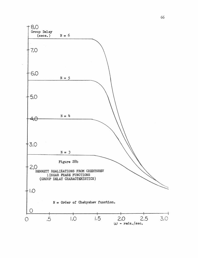
characteristics of the corresponding Bennett realizations are plotted in Figures 28a and b. The desired frequency interval over which the

phase was to remain linear was from 0 to 1,5 rps,, and the magnitude passband was fixed in the interval 0 to 1,0 rps, by the BENNET program.

Referring to Figure 28a, the greatest in-band magnitude ripple was obtained using the third order Chebyshev function in the Bennett

realization. This ripple was of the order of 0,006 dbs. Thus, the magnitude characteristics in the passband were very good. Outside

the passband, the attenuation cutoff rate was very slow up to W = 1.5 rps. Once again, as was the case with the Lemer filters, this seems to suggest a relationship between the group delay and the magnitude characteristics, since the group delay ceases to be linear attus 1.5

rps. In addition, as the order of the realization was increased, the stop-band attenuation began to have a faster cutoff rate, but it immediately dipped back down to less than half of the peak value. It

is possible that a parallel resonant corrector, such as in Lemer's approximation, could be placed in shunt with the load and source impedances to at least partially eliminate the out-of-band attenuation

dips. However, this measure was not attempted since this paper must be limited in its scope.

Referring to Figure 28b, the group delay characteristicsbehaved very well for all orders of the realization. The in-band

Attenuation(dbs.)

BENNETT REALIZATIONS FROM CHEBYSHEV LINEAR PHASE FUNCTIONS

(MAGNITUDE CHARACTERISTICS)

66

2,0 2,5l)J - rads./sec.

3,00 ,5 1,0 1.5

67

group delay ripple was negligible (probably due to the small ripple

of 0.050 degrees in the Chebyshev functions which were used). In addition, the group delay remained linear over the desired interval (from 0 to 1.5 rps.), verifying Bennett's realization procedure (Ref. i),

III. FINAL COMMENTS ON BENNETT'S APPROXIMATION

If one desires to obtain an equal-ripple magnitude response and a linear phase and have the ability to control the magnitude and linear phase passband intervals individually, the Bennett realiza­tion is tailored for the job. If one adds the further requirement of a fast cutoff rate, the Bennett realization will not meet that require­ment, This is especially true if the interval over which the phase is

to be linear is greater than the magnitude passband interval.

CHAPTER VII

LINEAR PHASE AND MAGNITUDE RELATIONSHIPS

IN A LATTICE NETWORK

I. DETERMINATION OF THE RELATIONSHIPS

The most logical thing to do when seeking the relationship between the phase and magnitude characteristics of a linear phase lattice network is to realize a linear phase filter in a lattice

configuration and observe the resulting magnitude. This was the procedure used in this research paper. Linear phase functions were realized in lattice form using the equation

G(s) = i(Ya - Ib)/(1 + Ya)(l + Yb) . (66)

The magnitude and phase characteristics of the resulting realization were determined using the computer program CXTLTC and CFRQRE (Ref. 3).

The Thomson, or maximally flat group delay approximation, was the first linear phase function which was realized (Ref. 5). The following is a simple third order realization, included to demonstrate the exact realization procedure utilized.

Realization of a Third Order Thomson Linear Phase Function in Lattice Form

Thomson funct, = s^ + 6s2 + 15s + 1 5 (6?)= (s + 2.3221854)(s + 1.8389073 ± jl.7543810) (68a.)= (s + 2.3221854)(s2 + 3.6778146s + 6.4594328) (68b)

69

If the above function had been of higher order, alternate poles would

have been associated with each of the two factors. Alternate poles have been associated in the two factors in Equation 68b above. From Equation 66

G(s) = £(Ya - Yb)/(1 + V ( 1 +Thus, using Equation 66 we obtain Equation 69.

3.6778146s - 2.3221854G(s) = --a t6 Ǥ.594 3 2 8 ___ s__

<s+2.8221854j (s^+ 3.6778146s + 6.4594328 s s2 + 6,4594328

(69)

andYa = 2.3221854/s (70)

Yb = 3.6778146s/(s2 + 6.4594328) (71)\ is readily realised as an inductor,

Ya = 1/0.43062884s (72)

Thus,L = 0.43062884 hy.

___________1___________Yb = ,27190060s + 1 (73)

.56937114sThus, Yb is a series LC circuit with

L = 0.27190060 hys.C = 0.56937114 fds.

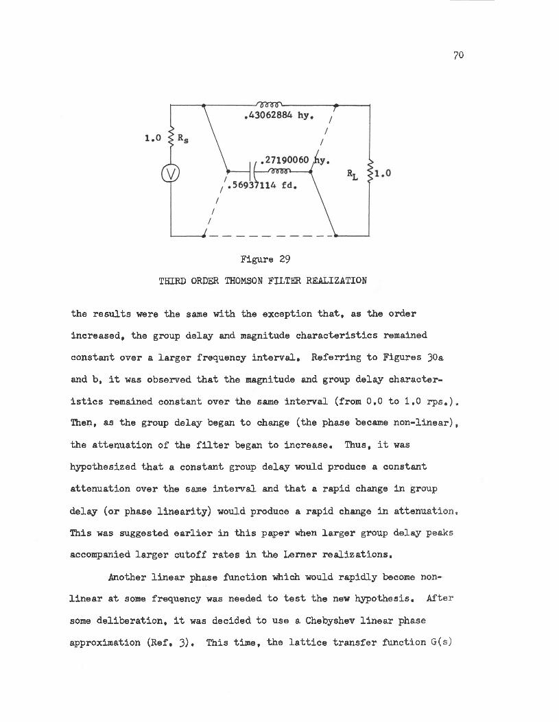
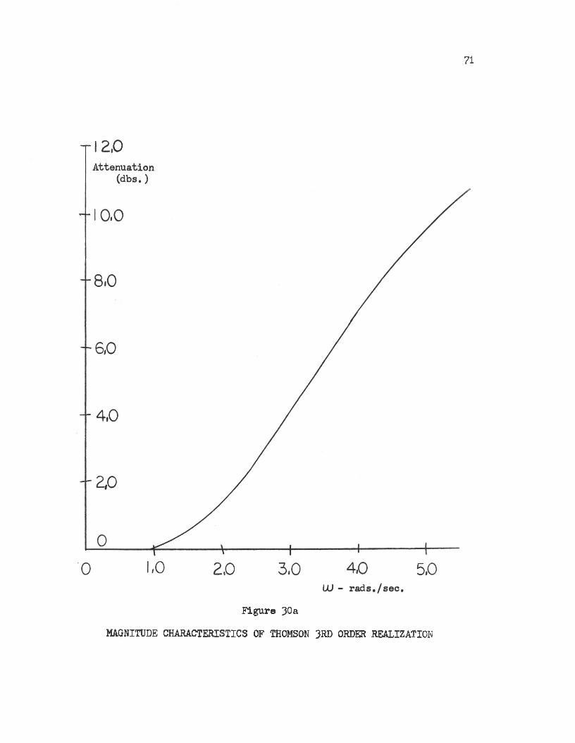
The final realization is sketched in Figure 29.The magnitude and phase characteristics of the maximally flat

delay realizations were then found using the computer program CXTLTC, mentioned earlier. The results for the third order function are plotted in Figures 30a and b. The higher order functions are not plotted,since

70

Figure 29THIRD ORDER THOMSON FILTER REALIZATION

the results were the same with the exception that, as the order increased, the group delay and magnitude characteristics remained constant over a larger frequency interval. Referring to Figures 30a

and b, it was observed that the magnitude and group delay character­istics remained constant over the same interval (from 0,0 to 1,0 rps.). Then, as the group delay began to change (the phase became non-linear),

the attenuation of the filter began to increase. Thus, it was hypothesized that a constant group delay would produce a constant attenuation over the same interval and that a rapid change in group

delay (or phase linearity) would produce a rapid change in attenuation. This was suggested earlier in this paper when larger group delay peaks accompanied larger cutoff rates in the Lemer realizations.

Another linear phase function which would rapidly become non­linear at some frequency was needed to test the new hypothesis. After

some deliberation, it was decided to use a Chebyshev linear phase approximation (Ref, 3)* This time, the lattice transfer function G(s)

71

Figure 30a

MAGNITUDE CHARACTERISTICS OF THOMSON 3RD ORDER REALIZATION

72

GROUP DELAY OF THOMSON 3RD ORDER REALIZATION

73

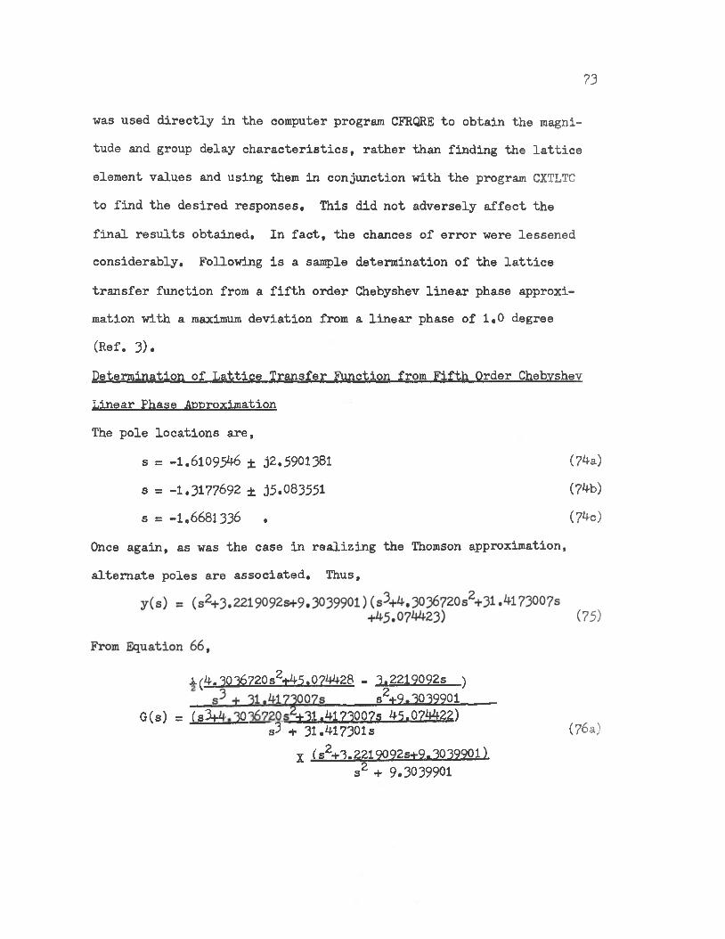
was used directly in the computer program CFRQRE to obtain the magni­tude and group delay characteristics, rather than finding the lattice element values and using them in conjunction with the program CXTLTC

to find the desired responses. This did not adversely affect the

final results obtained. In fact, the chances of error were lessened considerably. Following is a sample determination of the lattice

transfer function from a fifth order Chebyshev linear phase approxi­mation with a maximum deviation from a linear phase of 1,0 degree

Determination of Lattice Transfer Function from Fifth Order Chebyshev Linear Phase Approximation

The pole locations are.

Once again, as was the case in realizing the Thomson approximation, alternate poles are associated. Thus,

(Ref. 3).

s = -1,6109546 ± j2.5901381

s = -1.3177692 ± j5.083551 s = -1.6681336 .

(74a)(74b)(74c)

A-(4.3036720s2+45.074428 - 3.2219092s )____ s 2+9.3039901 .

G(s) = (sVtyj .T XI. .417300?g 45,07442.2)s3 + 31.417301s (76a)

X (s2+3.2219092s+9.30399011 s2 + 9.3039901

?4

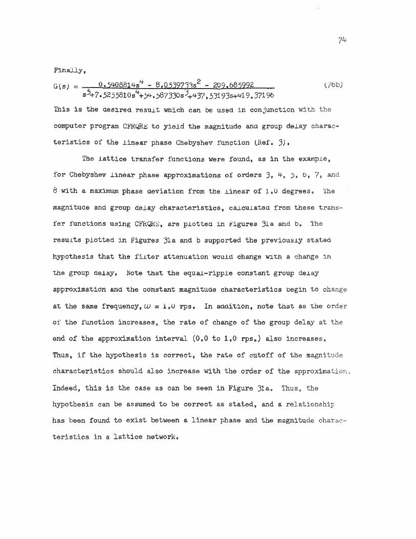
Finally,G(s; = 0.5 088148**’ - 8.0539733s2 - 209.685992 C76b)

s 5+?. 5255810s*l+3<+» 387330s +437,53193s+4l 9.37196This is the desired result wnich can be used in conjunction with the computer program CFRQRE to yield the magnitude and group delay charac­teristics of the linear phase Chebyshev function (Ref, 3).

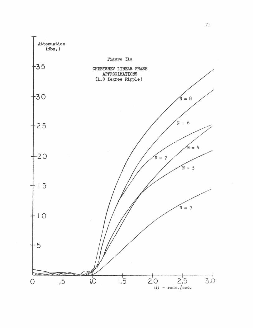
The lattice transfer functions were found, as in the example, for Chebyshev linear phase approximations of orders 3» 4, 3* b» 7. and 8 with a maximum phase deviation from the linear of 1,0 degrees. The

magnitude and group delay characteristics, ca.icuj.ated from these trans­fer functions using CFRQKE, are plotted in Figures 3la and b. The resuits plotted in Figures 31a and b supported the previously stated

hypothesis that the filter attenuation would change with a change in the group delay. Rote that the equal-ripple constant group delay

approximation and the constant magnitude characteristics begin to change

at the same frequency, U) = 1,0 rps. In addition, note tnat as the order of the function increases, the rate of change of the group delay at the

end of the approximation interval (0,0 to 1,0 rps.) also increases.

Thus, if the hypothesis is correct, the rate of cutoff of the magnitude characteristics should also increase with the order of the approximation.

Indeed, this is the case as can be seen in Figure 31a. Thus, the hypothesis can be assumed to be correct as stated, and a relationship has been found to exist between a linear phase and the magnitude charac­

teristics in a lattice network.

75

76

Group Delay (secs,)

CHEBYSHEV LINEAR PHASE APPROXIMATIONS (1,0 Deg. Ripple)

77

II. EXPERIMENTS WITH PRODUCING A GOOD IFDF APPROXIMATION USING THE OBSERVED PHASE AND MAGNITUDE RELATIONSHIPS

The rate of attenuation cutoff could be increased in the case of the Chebyshev linear phase approximations just discussed by increas­ing the group delay ripple, but even a 5*° degree phase ripple increased

the out-of-band attenuation by only 3*0 dbs. Thus, it would be intolerable in most cases to increase the phase ripple enough to yield

a satisfactory attenuation cutoff rate.It was noted that moving the last pole (at the high end of the

passband) of the Chebyshev approximation toward the jtu axis would produce a more rapid change in the group delay at the end of the approxi­

mation interval. Thus, the last pole of a fifth order function was moved in steps from its original location toward the jli> axis in an

attempt to increase the magnitude cutoff rate to better approximate an IFDF, The results are plotted as a family of curves in Figures 32a and b. As the pole was moved closer and closer to the jUJ axis, the group delay began to have a bump or peak on the band edge (bU = 1,0),

as can be seen in Figure 32b, This peak increased in magnitude as the pole was moved closer to the axis. This was the desired result since

such a change in the group delay should increase the magnitude cutoff rate at the band edge. Referring to Figure 32a, this was indeed the

case. The cutoff rate was much better than was the case with the original pole location (the characteristics of the original function are also plotted in Figures 32a and b), The results of moving this pole toward the jID axis appear to be analogous to the results obtained

78

Figure 32b79

CHEBYSHEV FIFTH ORDER FUNCTION WITH LAST POLE MOVED TOWARD

Group Delay juJ AXIS(secs. )

80

using Lemer's theory (see Figures 21a and b). There were a few by­products of moving the last pole toward the jU) axis, however, which adversely affected the passband. When the pole was moved to -0,6 and

-0.4 + 02835, a bump of magnitude 0,82 dbs, was obtained with<s~ = -0.6 and 1,4 dbs, with o~ = -0.4 near the high end of the passband. In addition, with c~ = -0,6 and -0,4, the cutoff rate was

very good, but the attenuation in the stop-band dipped back down to less than 25 dbs, from UJ = 1.5 rps. to UJ = 2,6 rps. for CT = -0,4 and less than 35 dbs. from UJ = 2,1 to UJ = 3»2 for o~ = -0,6. Such a dip could be intolerable for many applications. With the exception of the case when a~ = -0,4, the phase remained linear in an equal-

ripple sense (approximately 1.0 degree deviation) over approximately 85$ of the passband. This compares favorably with Lerner's approxi­mation (Ref. 4).

It is very probable that the addition of capacitors, for a low-

pass filter, or parallel LC circuits resonant at the center frequency, for bandpass filters, in shunt with the source and load impedances of a Chebyshev linear phase filter, with the last pole moved toward the

jUJ axis, could help clean up the passband and eliminate the stop-band dips in the attenuation. Such a corrector would be analogous to the corrector used by Lerner to reduce passband ripple and improve the

stop-band attenuation. Unfortunately, it is not within the scope of this paper to cover every possibility available for achieving good

approximations to the IFDF and ideal bandpass filter.One other method was used to approximate the IFDF characteristics

using the Chebyshev linear phase function. A series resonant circuit

was added in shunt with the A arm of the lattice to cause the admit-

81

tances of the A and B arms to approach one another at some predetermined frequency in the stop-band. This is analogous to the Y^ correctors in Lerner's filters, with the exception that the calculations required to find such a corrector for a Chebyshev approximation are much more cum­bersome .

After some careful thought, it was decided that the most convenient resonant frequency for the corrector resonance would be that frequency at or near the band edge. This decision was made,

because the lattice realization of a Chebyshev linear phase approxi­mation contains a series resonant circuit in the B arm which is reso­nant at the band edge frequency. This means that the A and B arm admittances will become approximately equal at that frequency and, thus, yield a high cutoff rate at the band edge.

Below is the lattice realization procedure used on a fifth order

Chebyshev function. From Equation 75. the lattice transfer function is4r4.303672QS2+45.0744228 - 3.2219092s )

s 3 + 31 >4173007s_______ s2 4- 9.3039901__________G(s) = ( s 4 4 , 30 36720s^+31.4173007s+45.074422)

s3 + 31.417301s "( s V 3 .2219092S+9.30 39901)

X s2 + 9.3039901Thus,

Ya = 3.2219092s/(s2 + 9.3039901)

Yb = (4.3036720s2 + 45.074428)/(s3 + 31.41730073s) Using Foster's second form (Ref. 3)

IB = 1.4347007/s + 2.8689713s/(s2 + 31.4173007; (80)

82

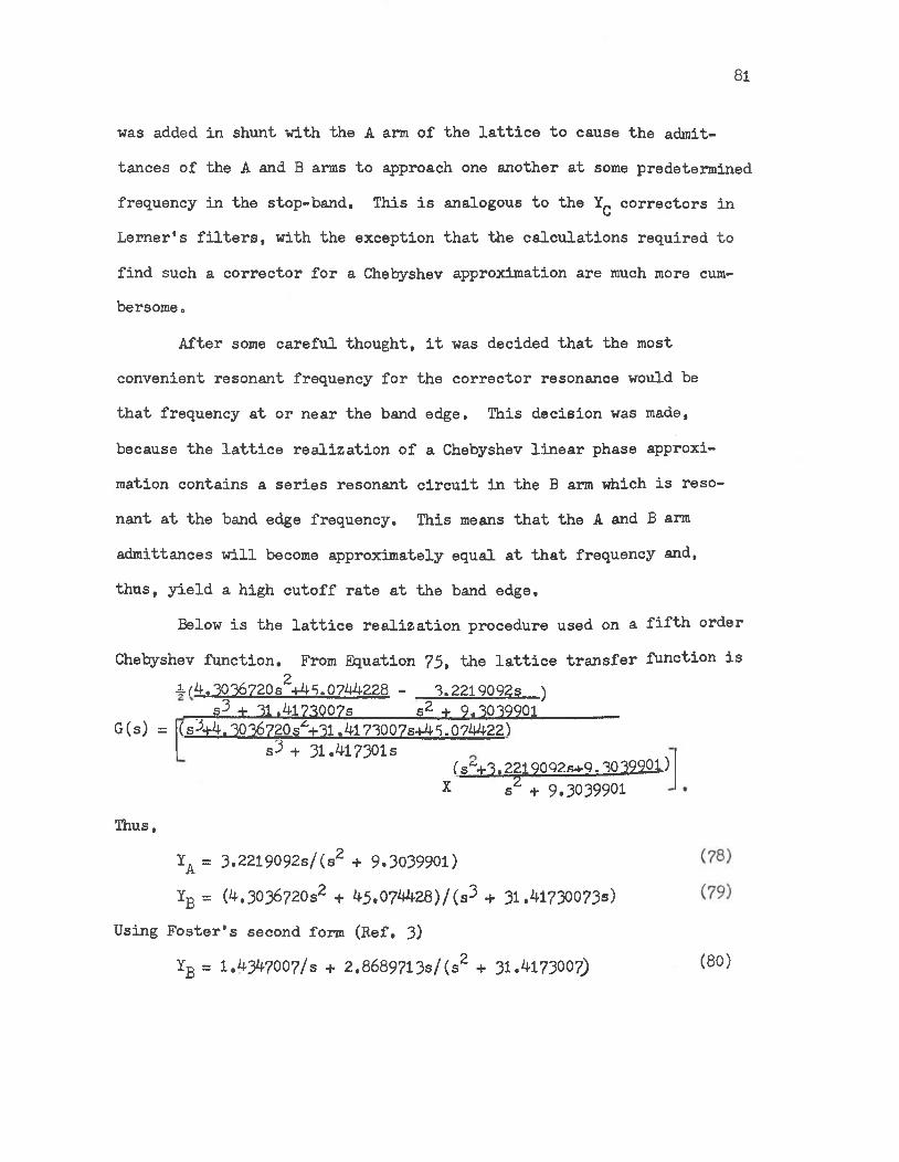
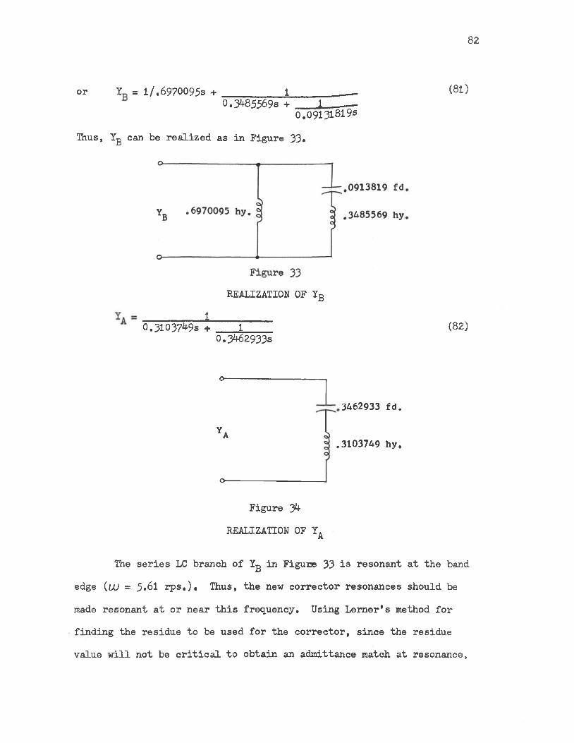
or Y = 1/. 6970095s + ___________1____________ (81)0.3485569s + 1 ----0.09131819s

Thus, Xg can be realized as in Figure 33«

REALIZATION OF Yfi

___________1___________0.31037^9s + 1 (82)

0.3462933s

o

YA

o

3462933 fd.

3103749 hy.

Figure 3- REALIZATION OF Y^

The series LC branch of Yg in Figure 33 is resonant at the band edge (uj = 5.61 rps,). Thus, the new corrector resonances should be

made resonant at or near this frequency. Using Lerner's method for finding the residue to be used for the corrector, since the residue value will not be critical to obtain an admittance match at resonance.

83

Residue = A = 4a/Tr R . (83)

5.0283551 (84)Equation 84 assumes the distance between the Chebyshev poles to be 2ac There are only two poles above the real axis, so the distance 4a will

be the distance from the real axis to the last pole (see Equations 74a, b, and c), Therefore,

A =1.6005752 (85)It was decided to place the corrector resonance at 5.6731512 rps.

since this is the frequency at which the linear phase approximation ends,

Y = (A/2)s/(s2 + 32.186445) (86)CSince A is not critical, A/2 will be rounded off to 0,800.Thus,

Yc = 0,800s/(s2 + 32.186445) (87)and

L = 1/0,800 = 1.2500 hys. (88)

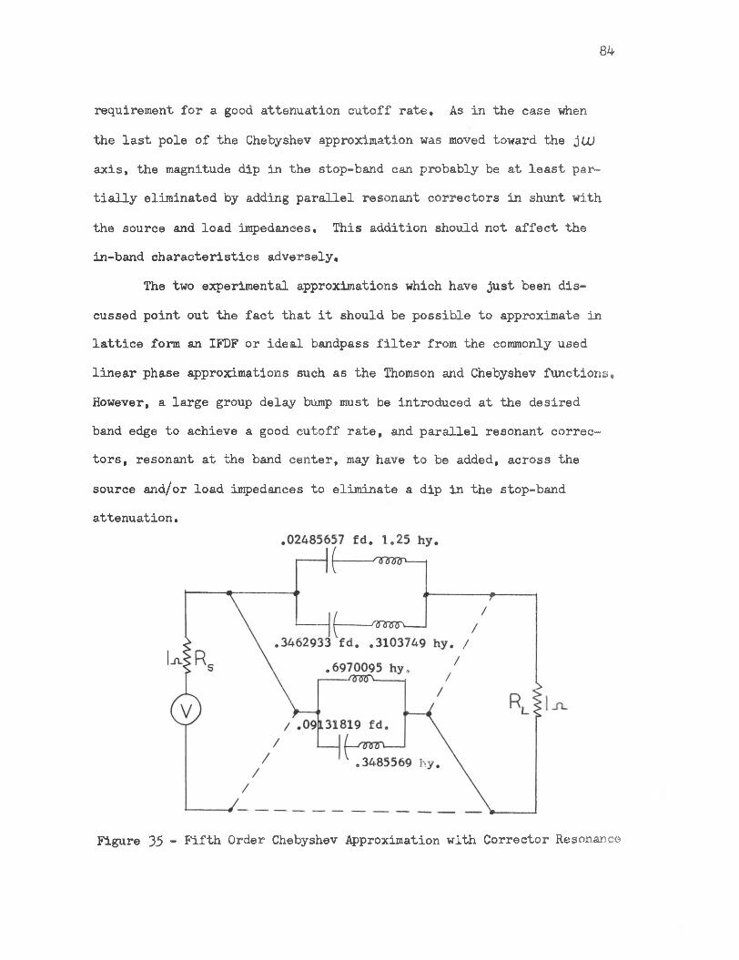
C = 0,800/32.184644 « 0.02485657 fds. (89)The complete lattice network is that of Figure 35*

The normalized magnitude and group delay characteristics (calcu­

lated using CXT.LTC) of this network are plotted in Figures 36a and b. Referring to Figure 36a, the in-band magnitude ripple was of the order of 0,30 dbs, and the stop-band attenuation was greater than 60 dbs, at UJ = 1.035 rps. The major problem with this approximation was that the stop-band attenuation dipped to 12 dbs, at LU = 1.1 rps. The phase linearity was very good in-band with the exception of the usual large

group delay bump at the band edge which has been shown to be the

8^

requirement for a good attenuation cutoff rate. As in the case when

the last pole of the Chebyshev approximation was moved toward the jLU axis, the magnitude dip in the stop-band can probably be at least par­tially eliminated by adding parallel resonant correctors in shunt with

the source and load impedances. This addition should not affect the in-band characteristics adversely.

The two experimental approximations which have just been dis­

cussed point out the fact that it should be possible to approximate in lattice form an IFDF or ideal bandpass filter from the commonly used

linear phase approximations such as the Thomson and Chebyshev functions. However, a large group delay bump must be introduced at the desired band edge to achieve a good cutoff rate, and parallel resonant correc­tors, resonant at the band center, may have to be added, across the

source and/or load impedances to eliminate a dip in the stop-band attenuation.

Figure 35 - Fifth Order Chebyshev Approximation with Corrector Resonance

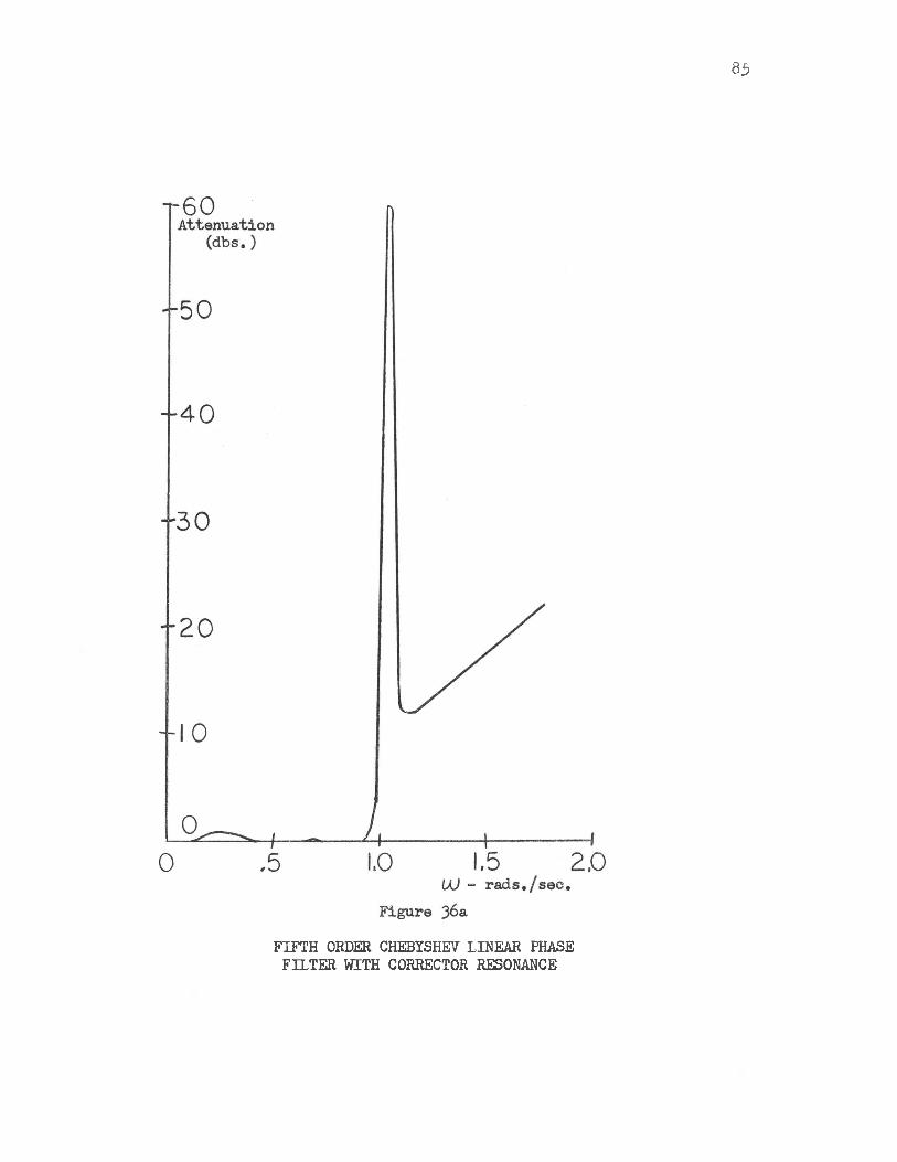
85

FIFTH ORDER CHEBYSHEV LINEAR PHASE FILTER WITH CORRECTOR RESONANCE

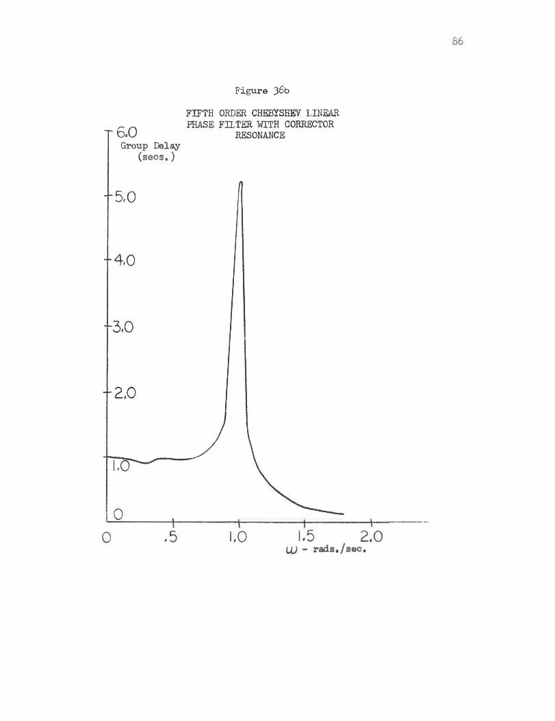
Figure 36b

FIFTH ORDER CHEBYSHEV LINEAR

CHAPTER VIII

CONCLUSIONS

Of all the IFDF and ideal bandpass filter approximations dis­

cussed in this paper, the Lerner approximation proved itself to be the closest to the ideal (Ref, 4), The cutoff rate of a Lerner filter can be rated as being in between that of the Butterworth and Chebyshev ideal magnitude approximations of the same order (Ref. 4), In addition,

the phase was linear over as much as 82# of the band (for an N of 11).As shown earlier, the Chebyshev, Butterworth, and Thomson functions

are intended to approximate either the ideal magnitude or ideal phase characteristics, but not both at the same time.

The Bennett realizations do a good job of approximating the ideal in the passband, but the attenuation cutoff rate and stop-band attenuation are far from being ideal. However, as mentioned earlier, it may improve the cutoff as well as the stop-band attenuation to add

a parallel resonant circuit across the source and load impedances of a Bennett filter in much the same manner as Lerner applied the correc­tor, Y^, On the other hand, Bennett's realizations do have one

advantage over the other filters discussed in this paper. That advan­

tage is the ability to control the magnitude and phase characteristics independently as far as the passband intervals are concerned (Ref, 1).

The IFDF approximations developed by the author appear to be

88

comparable to the Bennett realizations with the exception that they are much easier to realize than Bennett's. These approximations demonstrated that it is possible to approximate an IFDF using any linear phase function in lattice form using Equation 66 and possibly

adding a few correctors to clean up the stop-band attenuation charac­teristics.

Much work still remains to be done on developing better approxi­mations to the IFDF and ideal bandpass filter. The results in this paper indicate that the addition of corrector resonances to the existing linear phase functions, as well as juggling the positions of the poles

on the band edges of such functions, may open the door to several new approximations. The addition of such correctors and the moving of poles

would be guided by the relationship found in this paper between the linear phase and magnitude characteristics in a lattice network. The resulting non-minimum phase realizations would be hybrids of those existing at this time.

BIBLIOGRAPHY

1. B. J. Bennett, "Synthesis of Electric Filters with Arbitrary Phase

Characteristics," IRE Nat'l Conv. Rec.. Vol 1, Part 5» PP. 19-26}

1953.

2. W. L. C a sse ll, Linear E lec tr ic C ir c u its . John W iley & Sons, I n c ,,

New York, N.Y. s 1964.

3. D. Humpherys, "EE. 5 H and 512 Notes to be Published."

4. R. M, Lemer, "Band-Pass Filters with Linear Phase," Proc. IEEE, pp, 249-68? March, 1964.

5. L. Weinberg, Network Analysis and Synthesis. McGraw-Hill Book Co. Inc., New York, N.Y.$ 1962.„

6. W, C. Yengst, Procedures of Modern Network Synthesis. The MacmillanCo., New York, N.Y.s 1964

APPENDIX

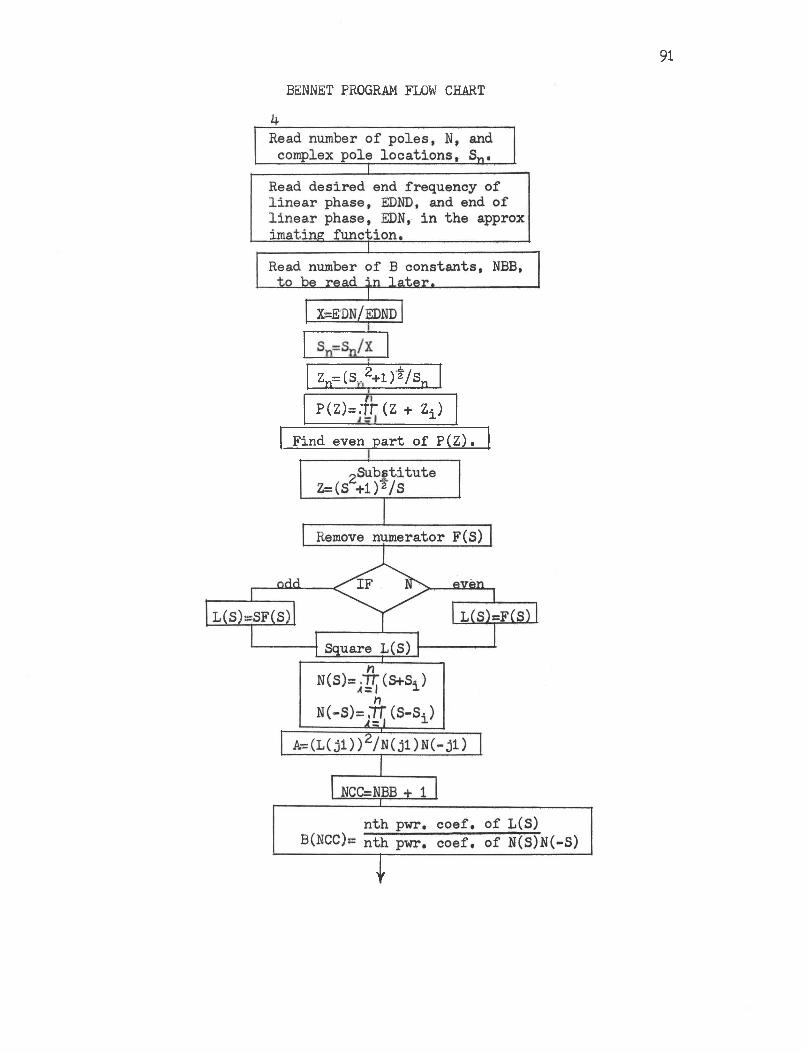
BENNET PROCRAM FLOW CHART

91

I Zn-(sAl)VsJ"p(z)=.-fr(z + zt)

Find even part of P(Z).

Y

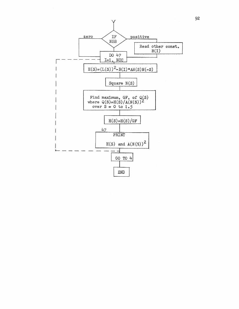
ABSTRACT

\

This thesis analyzed and compared several ideal bandpass filter approximations. In addition, the relationships between a linear phase

and the magnitude characteristics of a lattice filter were sought with the intention of using such relationships to develop a new approximation

to the ideal bandpass filter.Of the methods compared, Lemer's realization was found to be

the best approximation to the ideal bandpass filter. The Bennett

realization was found to have an unique property. That property was the ability to control the magnitude and phase passband intervals individually.

A relationship was found between a linear phase and the magni­tude characteristics of a lattice filter. It was found that a phase deviation from the linear produced a corresponding change in the

attenuation. The greater the phase deviation, the greater the attenu­ation change. From this relationship, two approximations to the IFDF were developed. Finally, it was determined that any good linear phase

function can be used to develop an approximation to either the IFDF or the ideal bandpass filter.