an analog accelerator for linear algebra - isca...
TRANSCRIPT

An Analog Acceleratorfor Linear Algebra
Yipeng Huang, Ning Guo, Mingoo Seok,Yannis Tsividis, Simha Sethumadhavan
Columbia University

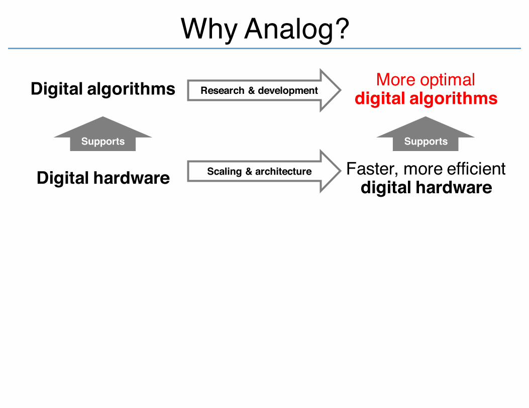
Why Analog?
Digital hardware
Digital algorithms
Supports
•Binary numbers
• Step-by-step operation

Why Analog?
Faster, more efficient digital hardware
Scaling & architectureDigital hardware
Digital algorithms
Supports
Why Analog?
Faster, more efficient digital hardware
More optimaldigital algorithms
Supports
Scaling & architecture
Research & development
Digital hardware
Digital algorithms
Supports

Why Analog?
Gates’ Simplification #1:Dennard scaling ended, Moore scaling will end
—Monday keynote speaker Doug Carmean
Faster, more efficient digital hardware
More optimaldigital algorithms
Supports
Scaling & architecture
Research & development
Digital hardware
Digital algorithms
Supports

Why Analog?
Analog hardware
Faster, more efficient digital hardware
More optimaldigital algorithms
Supports
Scaling & architecture
Research & development
Digital hardware
Digital algorithms
Supports

Why Analog?
Analog hardware
Analog algorithms
Supports
Faster, more efficient digital hardware
More optimaldigital algorithms
Supports
Scaling & architecture
Research & development
Digital hardware
Digital algorithms
Supports

Why Analog?
Analog hardware
Analog algorithms
Supports
Faster, more efficient digital hardware
More optimaldigital algorithms
Supports
Scaling & architecture
Research & development
Digital hardware
Digital algorithms
Supports
•No binary numbers•Continuous
operation

A continuous-time, analog computing model• step-by-step algorithm → continuous-time algorithm• continuous-time algorithm → analog accelerator hardware
Analog drawbacks: how to fix them• limited applications: tackle key linear algebra kernel• limited accuracy: calibration & exceptions• limited precision: build precision with digital help• limited scalability: divide & conquere sparse matrix
A prototype analog accelerator & evaluation• microarchitecture• architecture & programming• performance• energy

Analog computing solves ordinary differential equationsScientific computation phrased problems as ODEs
Modern problems are converted to linear algebra, not ODEsCan we accelerate linear algebra using analog?
Continuous-time algorithm

11
𝑨𝒙 = 𝒃

𝑨𝒙 = 𝒃
%𝑎00𝑥0 + 𝑎01𝑥1 = 𝑏0𝑎10𝑥0 + 𝑎11𝑥1 = 𝑏1
𝑥0
𝑥1

Direct methods• E.g., Gaussian elimination
Iterative methods
𝑨𝒙 = 𝒃
%𝑎00𝑥0 + 𝑎01𝑥1 = 𝑏0𝑎10𝑥0 + 𝑎11𝑥1 = 𝑏1
𝑥0
𝑥1

𝑨𝒙 = 𝒃
%𝑎00𝑥0 + 𝑎01𝑥1 = 𝑏0𝑎10𝑥0 + 𝑎11𝑥1 = 𝑏1
Direct methods• E.g., Gaussian elimination
Iterative methods• E.g., steepest gradient descent• E.g., conjugate gradients
𝑥0
𝑥1

Solve %𝑎00𝑥0 + 𝑎01𝑥1 = 𝑏0𝑎10𝑥0 + 𝑎11𝑥1 = 𝑏1
Step-by-stepsteepest gradient descent
𝑥0
𝑥1

Solve %𝑎00𝑥0 + 𝑎01𝑥1 = 𝑏0𝑎10𝑥0 + 𝑎11𝑥1 = 𝑏1
Step-by-stepsteepest gradient descent
recurrence relation
,𝑥-./0 = 𝑥-. − 𝑠 𝑎--𝑥-. + 𝑎-0𝑥0. − 𝑏- 𝑥0./0 = 𝑥0. − 𝑠 𝑎0-𝑥-. + 𝑎00𝑥0. − 𝑏0
𝑥0
𝑥1

Solve %𝑎00𝑥0 + 𝑎01𝑥1 = 𝑏0𝑎10𝑥0 + 𝑎11𝑥1 = 𝑏1
𝑥0
𝑥1
Continuous-timecontinuous steepest descent
𝑥0
𝑥1
Step-by-stepsteepest gradient descent
recurrence relation
,𝑥-./0 = 𝑥-. − 𝑠 𝑎--𝑥-. + 𝑎-0𝑥0. − 𝑏- 𝑥0./0 = 𝑥0. − 𝑠 𝑎0-𝑥-. + 𝑎00𝑥0. − 𝑏0

Solve %𝑎00𝑥0 + 𝑎01𝑥1 = 𝑏0𝑎10𝑥0 + 𝑎11𝑥1 = 𝑏1
𝑥0
𝑥1
Continuous-timecontinuous steepest descentordinary differential equation
%d𝑥- d𝑡⁄ = −𝑎--𝑥- − 𝑎-0𝑥0 + 𝑏- d𝑥0 d𝑡⁄ = −𝑎0-𝑥- − 𝑎00𝑥0 + 𝑏0
𝑥0
𝑥1
Step-by-stepsteepest gradient descent
recurrence relation
,𝑥-./0 = 𝑥-. − 𝑠 𝑎--𝑥-. + 𝑎-0𝑥0. − 𝑏- 𝑥0./0 = 𝑥0. − 𝑠 𝑎0-𝑥-. + 𝑎00𝑥0. − 𝑏0

CONTINUOUS-TIMEPotentially fast: not limited by step-by-step algorithm
A continuous-time, analog computing model

A continuous-time, analog computing model• step-by-step algorithm → continuous-time algorithm• continuous-time algorithm → analog accelerator hardware
Analog drawbacks: how to fix them• limited applications: tackle key linear algebra kernel• limited accuracy: calibration & exceptions• limited precision: build precision with digital help• limited scalability: divide & conquere sparse matrix
A prototype analog accelerator & evaluation• microarchitecture• architecture & programming• performance• energy

Datapath: explicit data flow
Values: represented as analog current & voltage
Functional units: analog arithmetic operators
Analog accelerator hardware

−𝑎10
−𝑎00
∫d𝑥1d𝑡 𝑥1(𝑡) ⍦
ADCDAC
∫d𝑥0d𝑡 𝑥0(𝑡)
ADCDAC
−𝑎11
−𝑎01
𝑏1
𝑏0 ⍦
∫d𝒙𝟏d𝒕 𝒙𝟏(𝒕)
∫d𝒙𝟎d𝒕 𝒙𝟎(𝒕)
Integrators
Solve %𝑎00𝒙𝟎 + 𝑎01𝒙𝟏 = 𝑏0𝑎10𝒙𝟎 + 𝑎11𝒙𝟏 = 𝑏1
ordinary differential equation
%d𝒙𝟎 d𝒕⁄ = −𝑎--𝒙𝟎 − 𝑎-0𝒙𝟏 + 𝑏- d𝒙𝟏 d𝒕⁄ = −𝑎0-𝒙𝟎 − 𝑎00𝒙𝟏 + 𝑏0

−𝑎10
−𝑎00
∫d𝑥1d𝑡 𝑥1(𝑡) ⍦
ADCDAC
∫d𝑥0d𝑡 𝑥0(𝑡)
ADCDAC
−𝑎11
−𝑎01
𝑏1
𝑏0 ⍦
ordinary differential equation
%d𝑥- d𝑡⁄ = −𝑎--𝑥- − 𝑎-0𝑥0 + 𝑏- d𝑥0 d𝑡⁄ = −𝑎0-𝑥- − 𝑎00𝑥0 + 𝑏0
∫d𝑥1d𝑡 𝑥1(𝑡) ⍦
∫d𝑥0d𝑡 𝑥0(𝑡) ⍦
Current mirrorfanout blocks

−𝑎10
−𝑎00
∫d𝑥1d𝑡 𝑥1(𝑡) ⍦
ADCDAC
∫d𝑥0d𝑡 𝑥0(𝑡)
ADCDAC
−𝑎11
−𝑎01
𝑏1
𝑏0 ⍦
ordinary differential equation
%d𝑥- d𝑡⁄ = −𝒂𝟎𝟎𝑥- − 𝒂𝟎𝟏𝑥0 + 𝑏- d𝑥0 d𝑡⁄ = −𝒂𝟏𝟎𝑥- − 𝒂𝟏𝟏𝑥0 + 𝑏0
−𝒂𝟏𝟎
−𝒂𝟎𝟎
∫d𝑥1d𝑡 𝑥1(𝑡) ⍦
∫d𝑥0d𝑡 𝑥0(𝑡) ⍦
−𝒂𝟏𝟏
−𝒂𝟎𝟏
Variablegain
amplifiers

−𝑎10
−𝑎00
∫d𝑥1d𝑡 𝑥1(𝑡) ⍦
ADCDAC
∫d𝑥0d𝑡 𝑥0(𝑡)
ADCDAC
−𝑎11
−𝑎01
𝑏1
𝑏0 ⍦
ordinary differential equation
%d𝑥- d𝑡⁄ = −𝑎--𝑥- − 𝑎-0𝑥0 + 𝒃𝟎 d𝑥0 d𝑡⁄ = −𝑎0-𝑥- − 𝑎00𝑥0 + 𝒃𝟏
−𝑎10
−𝑎00
∫𝑥1(𝑡) ⍦
DAC
∫𝑥0(𝑡) ⍦
DAC
−𝑎11
−𝑎01
𝒃𝟏
𝒃𝟎
Digital to analog converters

−𝑎10
−𝑎00
∫d𝑥1d𝑡 𝑥1(𝑡) ⍦
ADCDAC
∫d𝑥0d𝑡 𝑥0(𝑡)
ADCDAC
−𝑎11
−𝑎01
𝑏1
𝑏0 ⍦
ordinary differential equation
%d𝒙𝟎 d𝒕⁄ = −𝑎--𝑥- − 𝑎-0𝑥0 + 𝑏- d𝒙𝟏 d𝒕⁄ = −𝑎0-𝑥- − 𝑎00𝑥0 + 𝑏0
−𝑎10
−𝑎00
∫d𝒙𝟏d𝒕 𝑥1(𝑡) ⍦
DAC
∫d𝒙𝟎d𝒕 𝑥0(𝑡) ⍦
DAC
−𝑎11
−𝑎01
𝑏1
𝑏0
Sum currents
by joining wires

ordinary differential equation
%d𝒙𝟎 d𝒕⁄ = −𝑎--𝒙𝟎 − 𝑎-0𝒙𝟏 + 𝑏- d𝒙𝟏 d𝒕⁄ = −𝑎0-𝒙𝟎 − 𝑎00𝒙𝟏 + 𝑏0
−𝑎10
−𝑎00
∫d𝑥1d𝑡 𝒙𝟏(𝒕) ⍦
DAC
∫d𝒙𝟎d𝒕 𝒙𝟎(𝒕) ⍦
DAC
−𝑎11
−𝑎01
𝑏1
𝑏0
𝑥0
𝑥1
ADC
ADC

ordinary differential equation
%d𝑥- d𝑡⁄ = −𝑎--𝒙𝟎 − 𝑎-0𝒙𝟏 + 𝑏- d𝑥0 d𝑡⁄ = −𝑎0-𝒙𝟎 − 𝑎00𝒙𝟏 + 𝑏0
−𝑎10
−𝑎00
∫d𝑥1d𝑡 𝒙𝟏(𝒕) ⍦
ADCDAC
∫d𝑥0d𝑡 𝒙𝟎(𝒕) ⍦
ADCDAC
−𝑎11
−𝑎01
𝑏1
𝑏0
𝑥0
𝑥1

ordinary differential equation
%d𝑥- d𝑡⁄ = −𝑎--𝒙𝟎 − 𝑎-0𝒙𝟏 + 𝑏- d𝑥0 d𝑡⁄ = −𝑎0-𝒙𝟎 − 𝑎00𝒙𝟏 + 𝑏0
−𝑎10
−𝑎00
∫d𝑥1d𝑡 𝒙𝟏(𝒕) ⍦
ADCDAC
∫d𝑥0d𝑡 𝒙𝟎(𝒕) ⍦
ADCDAC
−𝑎11
−𝑎01
𝑏1
𝑏0
Solve %𝑎00𝒙𝟎 + 𝑎01𝒙𝟏 = 𝑏0𝑎10𝒙𝟎 + 𝑎11𝒙𝟏 = 𝑏1
𝑥0
𝑥1

CONTINUOUS-TIMEPotentially fast: not limited by step-by-step algorithm
ANALOG VALUESPotentially efficient: one wire carries real number
A continuous-time, analog computing model

A continuous-time, analog computing model• step-by-step algorithm → continuous-time algorithm• continuous-time algorithm → analog accelerator hardware
Analog drawbacks: how to fix them• limited applications: tackle key linear algebra kernel• limited accuracy: calibration & exceptions• limited precision: build precision with digital help• limited scalability: divide & conquere sparse matrix
A prototype analog accelerator & evaluation• microarchitecture• architecture & programming• performance• energy

Accuracy
Digital Analog
Intermediate values unambiguously interpreted as 1 or 0
Process & temperature variation → computation result variation!

Accuracy
Digital Analog
Intermediate values unambiguously interpreted as 1 or 0
Process & temperature variation → computation result variation!
Discrete math error correction possible
Within purely analog execution, no error correction

Components are inaccurate:• Gain• Offset• Nonlinearity (clipping)
Calibrate all components using additional DACs
Exceptions catch values exceeding valid input range
input
output
+Vs
-Vs
Accuracy: calibration & exceptions

Components are inaccurate:• Gain• Offset• Nonlinearity (clipping)
Calibrate all components using additional DACs
Exceptions catch values exceeding valid input range
input
output
+Vs
-Vs
Accuracy: calibration & exceptions

Components are inaccurate:• Gain• Offset• Nonlinearity (clipping)
Calibrate all components using additional DACs
Exceptions catch values exceeding valid input range
input
output
+Vs
-Vs
Accuracy: calibration & exceptions

Components are inaccurate:• Gain• Offset• Nonlinearity (clipping)
Calibrate: all components using additional DACs
Exceptions catch values exceeding valid input range
input
output
+Vs
-Vs
Accuracy: calibration & exceptions

Components are inaccurate:• Gain• Offset• Nonlinearity (clipping)
Calibrate: all components using additional DACs
Exceptions: catch values exceeding valid input range
input
output
+Vs
-Vs
validrange
Accuracy: calibration & exceptions

A continuous-time, analog computing model• step-by-step algorithm → continuous-time algorithm• continuous-time algorithm → analog accelerator hardware
Analog drawbacks: how to fix them• limited applications: tackle key linear algebra kernel• limited accuracy: calibration & exceptions• limited precision: build precision with digital help• limited scalability: divide & conquere sparse matrix
A prototype analog accelerator & evaluation• microarchitecture• architecture & programming• performance• energy

Precision: build precision w/ digital help
Limitation in sampling resolution→ limited precision result
𝑥0
𝑥1

Precision: build precision w/ digital help
Limitation in sampling resolution→ limited precision result
Find residual, rescale problem,& solve again in analog for precision
𝑥0
𝑥1𝑥0
𝑥1

A continuous-time, analog computing model• step-by-step algorithm → continuous-time algorithm• continuous-time algorithm → analog accelerator hardware
Analog drawbacks: how to fix them• limited applications: tackle key linear algebra kernel• limited accuracy: calibration & exceptions• limited precision: build precision with digital help• limited scalability: divide & conquere sparse matrix
A prototype analog accelerator & evaluation• microarchitecture• architecture & programming• performance• energy

Without time multiplexing, analog hardware needed for all variables• Impractical to build analog
hardware for whole problems
Solve subproblems of smaller size in analog• Possible because many
problems have sparse matrices
Scalability: divide & conquer sparse matrix

Without time multiplexing, analog hardware needed for all variables• Impractical to build analog
hardware for whole problems
Solve subproblems of smaller size in analog• Possible because many
problems have sparse matrices
Scalability: divide & conquer sparse matrix

A continuous-time, analog computing model• step-by-step algorithm → continuous-time algorithm• continuous-time algorithm → analog accelerator hardware
Analog drawbacks: how to fix them• limited applications: tackle key linear algebra kernel• limited accuracy: calibration & exceptions• limited precision: build precision with digital help• limited scalability: divide & conquere sparse matrix
A prototype analog accelerator & evaluation• microarchitecture• architecture & programming• energy• performance
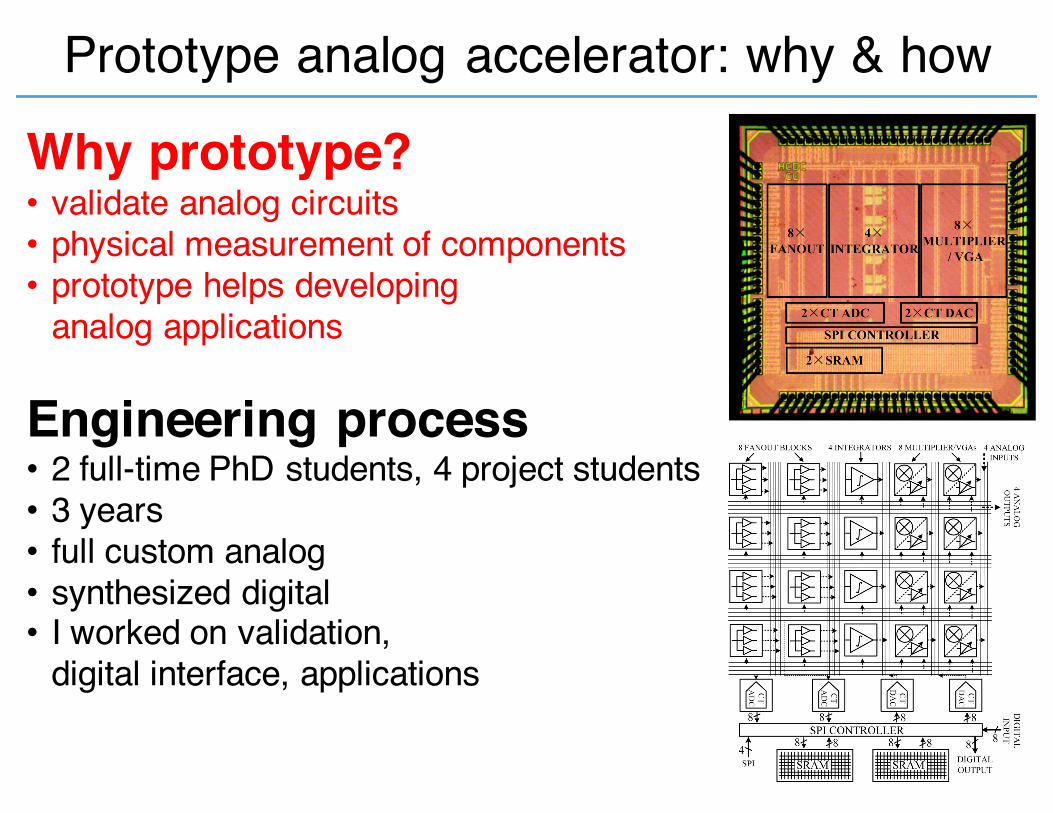
Prototype analog accelerator: why & how
Why prototype?• validate analog circuits• physical measurement of components• prototype helps developing
analog applications
Engineering process• 2 full-time PhD students, 4 project students• 3 years• full custom analog• synthesized digital• I worked on validation,
digital interface, applications

Prototype analog accelerator: μArch.
Components• 20 KHz analog bandwidth• 4 integrators• 8 multipliers• Other features: nonlinear lookup
Fabrication• 1.2 V 65nm TSMC• Low power density• 0.06 W/cm2 at full power• 2.0 mm2 active area• 1.2 mW at full power

Prototype analog accelerator: interface
Architecture• 8-bit A/D/A conversion• Configurable analog crossbar• Calibration & exceptions on all analog
Programming• Library for configuration• ODE syntax parser and compiler

A continuous-time, analog computing model• step-by-step algorithm → continuous-time algorithm• continuous-time algorithm → analog accelerator hardware
Analog drawbacks: how to fix them• limited applications: tackle key linear algebra kernel• limited accuracy: calibration & exceptions• limited precision: build precision with digital help• limited scalability: divide & conquere sparse matrix
A prototype analog accelerator & evaluation• microarchitecture• architecture & programming• energy• performance

50
Solution energy: analog HW vs. digital SW

0
100
200
300
0 100 200 300 400 500
Tim
e to
sol
utio
n (μ
s)
Number of variables
Digital solution time
Analog solution time
Solution time: analog HW vs. digital SW
10x less

0
100
200
300
0 100 200 300 400 500
Tim
e to
sol
utio
n (μ
s)
Number of variables
Digital solution time
Analog solution time
Solution time: analog HW vs. digital SW
Analog:• Explicit
dataflow architecture• Continuous-
time speed• Analog
efficiency• High analog
area cost

0
100
200
300
0 100 200 300 400 500
Tim
e to
sol
utio
n (μ
s)
Number of variables
Digital solution time
Analog solution time
Solution time: analog HW vs. digital SW
Analog:• Explicit
dataflow architecture• Continuous-
time speed• Analog
efficiency• High analog
area cost

0
100
200
300
0 100 200 300 400 500
Tim
e to
sol
utio
n (μ
s)
Number of variables
Digital solution time
Analog solution time
Solution time: analog HW vs. digital SW
Analog:• Explicit
dataflow architecture• Continuous-
time speed• Analog
efficiency• High analog
area cost

0
100
200
300
0 100 200 300 400 500
Tim
e to
sol
utio
n (μ
s)
Number of variables
Digital solution time
Analog solution time
Solution time: analog HW vs. digital SW
Analog:• Explicit
dataflow architecture• Continuous-
time speed• Analog
efficiency• High analog
area cost
Digital:• Optimal
digital algorithms

Continuous-time + analog offers alternative abstractions to digital
Tackled analog drawbacks: generality, accuracy, precision, scalability
Analog prototype: ISA & hardware; speed, area, energy analysis
Should we use analog to accelerate linear algebra?Some gains, but digital algorithms are optimized!Analog promises greater advantage in other problems: nonlinear?
An Analog Accelerator for Linear Algebra

57

58

Analog Digital
Continuous timeOrdinary differential equationAdvantage: fastAdvantage: low power b/c no clock
Discrete timeRecurrence relationAdvantage: allows complex algorithmsAdvantage: allows time multiplexing
Continuous valueCurrent & voltageAdvantage: fast and efficient operationsAdvantage: one wire carries real number
Discrete valueIntegers & floating pointAdvantage: high dynamic rangeAdvantage: high signal-to-noise ratio
59
𝑥0
𝑥1
𝑥0
𝑥1