Published in Image Processing On Line on 2015–07–29.Submitted on 2015–03–02, accepted on 2015–06–01.ISSN 2105–1232 c© 2015 IPOL & the authors CC–BY–NC–SAThis article is available online with supplementary materials,software, datasets and online demo athttp://dx.doi.org/10.5201/ipol.2015.131

2015/06/16

v0.5.1

IPOL

article

class

An Algorithmic Analysis of Variational Models for

Perceptual Local Contrast Enhancement

S. Ferradans1, R. Palma-Amestoy2, E. Provenzi3

1 ENS, CNRS, PSL, Paris, France (sira.ferradans@ens.fr)2 Woodtech Measurement Systems, Santiago, Chile (ropalma@ing.uchile.cl)

3 Laboratoire MAP5 (UMR CNRS 8145), Universite Paris Descartes, Paris, France(edoardo.provenzi@parisdescartes.fr)

Abstract

Color cast cancellation and local contrast enhancement are very important problems in computervision. In this paper we review the algorithm proposed by Palma-Amestoy et al. [A perceptuallyinspired variational framework for color enhancement, IEEE Transactions on Pattern Analysisand Machine Intelligence, 21 (2009), pp. 458–474], present results and evaluate the impact of achange in the parameters.

Source Code

The code implements the algorithm presented by Palma-Amestoy et al. [7], with a pre-computation of the polynomials. These polynomials are inputted from text files which are alsoprovided.

The reviewed source code and documentation for this algorithm are available from the webpage of this article1. Compilation and usage instruction are included in the README.txt file ofthe archive.

Supplementary Material

As supplementary material, a reference dataset is provided, and the Matlab code to generatethe polynomial approximation, although it is not necessary to execute it to test the algorithm.

Keywords: color constancy; contrast enhancement; Weber-Fechner contrast; visual adapta-tion; human visual system.

1http://dx.doi.org/10.5201/ipol.2015.131

S. Ferradans, R. Palma-Amestoy, E. Provenzi , An Algorithmic Analysis of Variational Models for Perceptual Local Contrast Enhancement,Image Processing On Line, 5 (2015), pp. 219–233. http://dx.doi.org/10.5201/ipol.2015.131

S. Ferradans, R. Palma-Amestoy, E. Provenzi

1 Introduction

In this paper, we will consider the problem of local contrast enhancement inspired by human percep-tion and its consequences on color cast removal. More specifically, given any digital image, acquiredunder general illumination conditions, we will try to modify its chromatic attributes so that theresulting image is as close as possible to the human perception of the scene photographed in thepicture.

This kind of algorithms are of great importance in different fields that need an illumination-independent representation of the scene such as object recognition, calibration, image segmentationor tracking. They have also proven necessary in computational photography and flickering reduction,to quote but two applications.

In [7] the authors built a general variational framework to perform perceptual color correction.Their work is based on the selection of energy functionals through suitable constraints related tophenomenological properties of the Human Visual System (HVS).

This variational framework allows to embed existing perceptual color correction algorithms andclarify more easily the main similarities and differences among them. The usefulness of this resultrelies in the fact that the direct equations of these algorithms are very distant from each other, butnot the energies they minimize.

The plan of this paper is the following: in Section 2, we introduce the perceptual laws and themathematical model behind the algorithm. In Section 3, we detail the numerical scheme and presentthe final algorithm. Finally, in Section 4, we present some results and how they vary when changingthe default parameters.

2 A General Variational Framework for Perceptual Color

Correction

In this section, we will introduce the basic results of paper [7]. First of all, we will introduce anddiscuss the meaning of an important result on the variational interpretation of histogram equalization(HE), which is strongly related to the framework proposed in [7]. Then, we will briefly recall fourbasic HVS features, and, finally, we will show how to modify the energy function of HE in order totake into account these HVS characteristics, which is one of the main results of [7].

Before going through this description, we introduce the notation that will be used in the restof the paper. Let us denote with Ω ⊂ R2 the spatial domain of a digital image, with |Ω| its areaand with x ≡ (x1, x2) and y ≡ (y1, y2) the coordinates of two arbitrary pixels in Ω. We will alwaysconsider a normalized dynamic range in [0, 1], so that a RGB image function will be denoted with

~I : Ω −→ [0, 1]× [0, 1]× [0, 1]x 7→ (IR(x), IG(x), IB(x)),

where each scalar component Ic(x) defines the intensity level of the pixel x ∈ Ω in the red, green andblue channels, respectively.

We stress that we will perform every computation on the scalar components of the image, thustreating each chromatic component separately. Therefore, we will avoid the subscript c and writesimply I(x) to denote the intensity of the pixel x in a given chromatic channel.

2.1 Variational Interpretation of Histogram Equalization

One of the main inspirations of paper [7] was the following result about the variational interpretationof histogram equalization [11].

220

An Algorithmic Analysis of Variational Models for Perceptual Local Contrast Enhancement

Theorem 1 : Histogram equalization can be implemented by minimizing the following energy

Ehist eq(I) ≡ 2

∫Ω

(I(x)− 1

2

)2

dx − 1

|Ω|

∫∫Ω2

|I(x)− I(y)| dxdy. (1)

Let us write the HE energy functional as follows: Ehist eq(I) = D 12(I) − C(I), where the two

functional terms D 12(I) and C(I) are

D 12(I) ≡ 2

∫Ω

(I(x)− 1

2

)2

dx, (2)

and

C(I) ≡ 1

|Ω|

∫∫Ω2

|I(x)− I(y)| dxdy. (3)

The minimization of Ehist eq(I) = D 12(I) − C(I) is achieved through the minimization of D(I) and

−C(I) (i.e. the maximization of C(I)).

Dispersion term. D 12(I) is called global quadratic dispersion term around the middle gray level

1/2 and it is minimized when I(x) ≡ 1/2 for all x ∈ Ω, i.e. the minimization of this term tends toturn I into a uniform gray image.

Contrast term. C(I) is called global contrast term and its maximization corresponds to the inten-sification of the global contrast of the image I, measured through the absolute differences |I(x)−I(y)|.

Optimization. The main result of paper [11] is that, if I∗ = argminI Ehist eq(I), then I∗ hasequalized histogram, i.e. all the intensity levels have the same occurrence probability in the image.In [11], the authors prove this result by showing that, if we denote by H the cumulative histogram,then the image function I∗ satisfies the equation H(I∗(x)) = I∗(x), for all x ∈ Ω, which implies theflatness of the histogram of I∗, see e.g. [4].

The minimization of Ehist eq(I) can be achieved through gradient descent. With respect to this,another important result of [11] is that, if I0 represents any input image, then the initial valueproblem

∂tI = −δEhist eq(I)

I(0) = I0

, (4)

has only one solution, where t is the evolution parameter of the iterative gradient descent schemeand the symbol δ represents the first variation of the functional.

Interpretation. The argmin of Ehist eq(I) is the image corresponding to the optimal balance be-tween two opposite effects : on one side, the minimization of D 1

2(I) tends to set all the levels to the

average gray 1/2 but, on the other side, the minimization of −C(I) tends to spread the intensitylevels apart, as far as possible from each other.

So, the intrinsic meaning of the variational description of histogram equalization is that theequilibrium among two conflicting actions, control of the intensity dispersion around the middle graylevel and contrast enhancement, induces histogram equalization.

One practical consequence of this result is that, applying for example the gradient descent tech-nique to minimize Ehist eq(I), one can stop the minimization process before reaching the completeequalization, thus realizing a partial equalization that can nonetheless be useful to avoid the typicalover-enhancement of low-key images (see [4] for more details).

221

S. Ferradans, R. Palma-Amestoy, E. Provenzi

However, for the purposes of color image processing, the most important consequences of Theorem1 are theoretical: in fact, as we will see in the next section, we can modify the functional Ehist eq(I)in such a way that the basic principle of histogram equalization, i.e. the balance between dispersioncontrol and contrast enhancement, is preserved but we can change the analytical form of the termsD 1

2(I) and C(I) taking inspiration from human visual perceptual features. The argmin image I∗

of the modified functional is a color-corrected version of the original image driven by perceptualproperties of the HVS.

2.2 A Basic Set of Four Basic HVS Properties

The HVS is an extraordinarily complex system, nowadays still far from being fully understood. As itwould be impossible to provide an even approximate description, here we will just recall the four basicphenomenological mechanisms of color vision that will be used to select perceptual functionals. Asa general reference for the following subsection, the reader can refer to the very complete book [13].

2.2.1 Adaptation to the Average Luminance Level

The absortion of a photon by one of the three L,M, S cones activates a photo-chemical transductionprocess which transforms the electromagnetic energy of the photon to a difference of electric potentialof the photoreceptor’s membrane.

The empirical law that describes this transduction, see e.g. [12], is known as Michaelis-Menten’sequation (or Naka-Rushton’s equation when the coefficient n is unitary)

r(L) =∆V

∆Vmax

=Ln

Ln + LnS, (5)

where ∆Vmax is the highest difference of potential that can be generated, n is a constant (measuredas 0.74 for the rhesus monkey), L is the luminance of the viewed object and LS is the luminanceat which the photoreceptor response is half maximal, called the semisaturation level, and whichis usually associated with the level of adaptation. Each type of cone L,M, S is most sensitive in aparticular waveband and the semisaturation constant depends on the amount of light in the particularwaveband that is absorbed, not on the global luminance of the light source.

Equation 5 has a sigmoid-like behavior that can be interpreted as follows: the photoreceptorsresponse has an intensity threshold, below which their output is null, then they respond fairly linearlyand, finally, the response saturates as we approach large values of luminance.

The ‘center’ of this behavior is the semisaturation value LS, which is mapped to 1/2, in this sensethe retinal cells ‘adapt’ to each scene average luminance, allowing us to perceive modulations of lightintensity around LS. This adaptive capacity of retinal cells is of paramount importance for humanvision, without it we simply would not be able to see when passing from a dim light environment toa very intensely illuminated one, and viceversa.

2.2.2 Local Contrast Enhancement

The HVS operates a local contrast enhancement, with the primary (but not the only) effect ofimproving edge perception, as proven by visual effects as simultaneous contrast or Mach bands, seee.g. [4]. Edges contain the most important part of the visual information, so it is not surprising thatthe HVS has developed a way to improve their perception. The most important feature that mustbe underlined here is that edge enhancement is local, i.e. it depends on the local distribution of lightintensity around each point.

222

An Algorithmic Analysis of Variational Models for Perceptual Local Contrast Enhancement

2.2.3 Color Constancy

If light adaptation is the HVS ability to adapt to different light intensities, color constancy may bedescribed at first glance as the ability to adapt to different light spectral content, in order to perceivecolors as constant as possible to changes in illumination. This feature is so intrinsically hardwired inour visual system that we often take it for granted. However, whenever we take two pictures of thesame scene with two different illuminants, we see that we must perform a very careful white balanceto obtain two images that produce similar color sensations. The psycho-physiological details thatallow color constancy are beyond the scopes of this work, for more details see e.g. [5].

Color constancy will be essential for the selection of the analytical form of the contrast enhance-ment term of perceptual functionals.

2.2.4 Weber’s Law

Weber’s psychophysical experiments to test contrast perception consist in what follows: a dark-adapted human observer is put in a dim room in front of a white screen on which a narrow beam oflight is thrown in the center of the visual field. The luminous intensity I of the beam is increasedvery slowly and the observer is asked to tell whether he/she can perceive an intensity change. Theleast perceptible intensity change ∆I is generally called JND for Just Noticeable Difference.

Weber found that the JND increases proportionally with the luminous intensity, i.e. ∆I = K · I,or, as it is in general reported

∆I

I' K. (6)

Equation (6) is called Weber’s law and K Weber’s constant. Weber’s law says that, as we increase thebackground light I, the difference ∆I must increase proportionally in order to be able to appreciateI + ∆I as different from I.

2.3 Variational Perceptually-Inspired Color Correction of Digital Im-ages

In [7] the perceptual features recalled in Subsection 2.2 have been used to modify the histogramequalization functional described in Subsection 2.1 as reported in the next theorem.Theorem 2 : The only class of energy functionals complying with all the four HVS features discussedin Section 2.2 is the following

Eµ,I0,w,ϕ(I) = Dµ,I0(I) + Cw,ϕ(I), (7)

where

Dµ,I0(I) =

∫Ω

[α

(µ log

µ

I(x)− (µ− I(x))

)+ β

(I0(x) log

I0(x)

I(x)− (I0(x)− I(x))

)]dx, (8)

and

Cw,ϕ(I) =

∫∫Ω2

w(x, y)ϕ

(minI(x), I(y)maxI(x), I(y)

)dxdy, (9)

where:

• I0 is a given channel of the original image function;

• µ is the average value of I0;

223

S. Ferradans, R. Palma-Amestoy, E. Provenzi

• α, β > 0 are real coefficients which control the attachment to µ and to the original imagefunction values I0, respectively;

• w : Ω × Ω → R+ is a spatial kernel, which depends only on the Euclidean distance ‖x − y‖between two generic pixels x, y ∈ Ω and it is monotonically decreasing with the distance itself,i.e. w(x, y) := g(‖ x− y ‖) where g : R+ → R is monotonically decreasing;

• ϕ : [0, 1]→ R is a monotonically increasing differentiable function.

Contrast Term and Color Constancy. To understand the motivation for the analytical shapeof the contrast term Cw,ϕ(I) let us consider the basic image formation model, i.e. I(x) = ρ(x) · λ,where ρ(x) represents the reflectance of a point x and λ represents the illuminant (supposed to beconstant all over the scene). Since Cw,ϕ(I) is written in terms of a ratio, it is evident that it isindependent from illuminant changes, thus it is coherent with the color constancy feature. Moreover,as proven in [7], this analytical form is the only one in which color constancy and Weber’s law canbe combined.

Function ϕ represents a degree of freedom and it is chosen to be monotonically increasing toprevent contrast reversion between pixels.

Contrast Term and Local Contrast Enhancement. Finally, notice that the minimization ofCw,ϕ(I) indeed induces a contrast enhancement. In fact, the ratio minI(x), I(y)/maxI(x), I(y)is minimized when the lowest value between two pixels is decreased and the highest is increased,which, of course, corresponds to an intensification of contrast. The enhancement is spatially localdue to the presence of the weighting function w. Typically w is a Gaussian kernel with center inx, its standard deviation σ can be set by the user to increase or decrease the locality of contrastenhancement. Small values of σ push the effect towards sharpening, large values of σ instead pushtowards a global enhancement.

Dispersion Term. The choice of the dispersion term has been guided by dimensional coherencewith the contrast term, which has dimension 0 with respect to I. The easiest meaningful candidateis the entropy functional Dµ,I0 , whose minimization produces a reduction of entropy, i.e. disorder,around the average value µ (which can be different in each chromatic channel) and around theoriginal image I0. This last attachment is introduced to avoid an excessive departure from theoriginal intensity values and can be modulated via the coefficients ratio α/β. To understand whyDµ,I0 complies with the tasks of a dispersion term, we note that the abstract analytical form of theintegrand can be written as f(s) = a log a

s− (a − s) [1], where s ∈ (0, 1] is a generic normalized

intensity level and a > 0 can represent either µ or I0(x). The first derivative of f(s) is dfds

(s) = 1− as,

so dfds

(s) = 0 if and only if s = a. Moreover, the second derivative is d2fds2

(s) = as2> 0, ∀s. This

implies that the value s = a is a global minimum for f(s). Hence, minimizing Dµ,I0 corresponds toan attachment to µ and around the original data I0(x).

2.4 Relationship with Existing Perceptually-Inspired Color CorrectionModels

If we compare Ehist eq with Eµ,I0,w,ϕ(I), we can infer that a perceptually-inspired color correctioncan be interpreted as a suitable local and non linear version of histogram equalization. Moreover,within this framework, it is possible to link two well-known models for perceptually-inspired colorcorrection ACE [10] and Retinex [6]. As previously said, this result is quite remarkable, since theoriginal equations of ACE and Retinex seem to be very distant from each other, see [8] and [9] for

224

An Algorithmic Analysis of Variational Models for Perceptual Local Contrast Enhancement

more details. This can be done simply by selecting two different analytical expressions of the functionϕ. In [3] and [2], respectively, it has been proved that:

• If ϕ ≡ log, then the minimization of Eµ,I0,w,log(I) leads to the so-called ACE algorithm formu-lated in [10];

• If ϕ ≡id, then the minimization of Eµ,I0,w,id(I) leads to the continuous symmetrized version ofthe original Retinex algorithm [6].

In the test section, apart from the identity and the logarithmic function, we will also consider

the following choice of ϕ ≡ −M, where M(

min(I(x),I(y))max(I(x),I(y))

):=

1− min(I(x),I(y))max(I(x),I(y))

1+min(I(x),I(y))max(I(x),I(y))

≡ |I(x)−I(y)|I(x)+I(y)

, which corre-

sponds to a novel algorithm.

3 Algorithm

3.1 Stability of the Numerical Scheme for the Minimization of Percep-tual Functionals

The Euler-Lagrange equations of Eµ,I0,w,ϕ(I), i.e. δEµ,I0,w,ϕ(I) = 0, are integral equations that cannotbe solved analytically. Moreover, the perceptual functionals are not convex, so we cannot easily find aglobal minimum. However, in [7] it has been proved that, if we substitute the null values of the inputimage with 1/255 (the smallest non-zero value in the normalized dynamic range), and we considerα, β > 1, then the gradient descent scheme with respect to log I, i.e.

∂t log I = −δEµ,I0,w,ϕ(I), (10)

converges to a unique image function, that we can consider the perceptually-inspired color-correctedone. The gradient descent is written in terms of log I because the logarithmic derivative, i.e. ∂t log I =1I∂tI allows re-writing the gradient descent equation as follows

∂tI = −I · δEµ,I0,w,ϕ(I), (11)

the right-hand side of this equation has dimension 0 (which is the correct perceptual dimension),since δEµ,I0,w,ϕ(I) has dimension2 -1 in terms of I. Moreover, notice that, as proved in [1], the effectof taking the logarithmic image is simply to change the speed of convergence of the gradient descentscheme and not its final result.

Discretization. Defining a finite evolution step ∆t and setting Ik+1(x) = Ik∆t(x) for k = 0, 1, 2, . . .,from (11) we obtain the following minimization scheme

Ik+1(x) =Ik(x) + ∆t

(αµ+ βI0(x) + 1

2Cϕw,k(x)

)1 + ∆t(α + β)

, (12)

where

Cϕw,k(x) =∑y∈Ω

w(‖x− y‖)ϕ(

minIk(x), Ik(y)maxIk(x), Ik(y)

). (13)

2In general, the first variation of a homogeneous functional of degree n is a homogeneous functional of degree n−1,in our case Eµ,I0,w,ϕ(I) has degree 0, so its first variation has degree -1.

225

S. Ferradans, R. Palma-Amestoy, E. Provenzi

3.2 Complexity Reduction of the Contrast Term

The computational complexity of these algorithms is O(N2), N being the number of pixels in theimage. This high complexity is due to the contrast term: its first variation generates the integralterm Cϕw,k(x) in the Euler-Lagrange equations. We present now the approximation technique proposedin [7] to reduce the computational complexity to O(N logN).

The basis of the complexity reduction technique is to write Cϕw as an expression that separatesthe dependence between I(x) and I(y). Let us drop the dependence on the iteration k in this sectionfor the sake of simplicity. We rewrite the generic contrast term in the following way

Cϕw(x) = f(I(x))∑y∈I

w(‖x− y‖)g(I(y)). (14)

By definition, the sum in the previous formula is a convolution, thus we just need to find the functionsf and g. Let p be a generic polynomial of order n on the variables I(x), I(y)

p(I(x), I(y)) =n∑j=0

j∑m=0

pj−m,mI(x)j−mI(y)m =n∑j=0

fj(I(x))I(y)j, (15)

setting g(I(y)) = Ij(y), we can express the contrast term as

C[ϕ,n]w (x) =

n∑j=0

fj(I(x))(w ∗ Ij)(x), (16)

where fj(I(x)) =∑n−j

m=0 pm,jIm(x), and ∗ is the convolution operator. We compute the coefficients

fj of the polynomial of order n by solving p[ϕ,n](I(x), I(y)) = argminp ‖p − ϕ‖2, i.e. p[ϕ,n] is thepolynomial of order n with minimal quadratic distance with respect to the function ϕ.

Numerical Algorithm. Note that the coefficients fj depend on the intensity of the pixel thusthey can be precomputed for a meaningful discrete number of values. See Algorithm 1 for moredetails. The degree n of the polynomial is a parameter that controls the precision of the polynomialapproximation. For all numerical tests, it was set to n = 9 which amounts to a number of coefficientsC = 55.

3.3 Final Algorithm

The numerical scheme (12) accelerated with the complexity reduction approach is detailed in Algo-rithm 2. In practice, this algorithm is applied to each color component independently.

Restrictions on the parameters α, β. Regarding the parameters ∆t, α and β, it is important toanalyze their restrictions to guarantee the algorithm convergence. Let us set ∆t ∈ [0, 1] and µ = 1

2.

The basic condition for convergence is to keep Ik+1(x) ∈ [0, 1] at each step, which can be done byanalyzing the boundary intensity values of Equation (12). The minimal value of the pixel Ik+1(x) isobtained when all the equation components are minimal

Ik+1(x) =∆t(

12α− 1

2

)1 + ∆t(α + β)

≥ 0, (17)

which leads to the condition α ≥ 1, since β ≥ 0. The analysis on the maximal value Ik+1(x) ≤ 1confirms this condition on α.

226

An Algorithmic Analysis of Variational Models for Perceptual Local Contrast Enhancement

Algorithm 1: Polynomial coefficients computation

Input: Type of contrast c = id, log,−M.Output: p[ϕ,n] = pciCi=0, where C is the number of coefficients of the polynomial of degreen = 9.

1. Range x = 1255, 2

255, . . . , 255

255 and y = 1

255, 2

255, . . . , 255

255

2. Approximation of the sign function sε(z) = arctan(z/ε)arctan (1/ε)

, where ε = 1/20.

3. Set contrast function ϕ

• if c = id then ϕid(x, y) = xymaxε(x,y)

sε(x− y)

• if c = log then ϕlog(x, y) = sε(x− y)

• if c = −M then ϕ−M(x, y) = 2xy(x+y)2

sε(x− y)

4. Fit coefficients Solve the following least squares problem:p[ϕc,n] = arg minp ‖

∑nj=0

∑jm=0 pj−m,mx

j−lyl − ϕc(x, y)‖2.

Algorithm 2: Contrast enhancement

Input:

- I0(x) ∈ [0, 1]: input image, where x ∈ Ω is the number of pixels.

- c : type of contrast id, log,−M

- σ: weight parameter,

- α ≥ 1, β ≥ 0: importance of the attachment to 12

and I0, respectively.

Output: Ik

1. Compute Polynomials: Find p[ϕc,n] with Algorithm 1 with c as the parameter.

2. Weighting function: Precompute wσ(x, y) with equations (18) or (19)

3. Set constants: ∆t = 0.02, µ = 12

and proj[a,b](x) = max(min(x, b), a)

4. Optimization: Iterate until convergence: while ‖Ik+1 − Ik‖2 > ε

• Precompute: W jk = w ∗ Ijk, for j = 1, . . . , n

• For every pixel x ∈ Ω :

– C[ϕc,n]w,k (x) = proj[−1,1]

(∑nj=0

∑n−jm=0 p

cm,jIk(x)mW j

k (x))

– Ik+1(x) = proj[0,1]

(Ik(x)+∆t

(αµ+βI0(x)+ 1

2C[ϕ

c,n]w,k (x)

)1+∆t(α+β)

)

Note that it has been assumed that the contrast component∑n

j=0

∑n−jm=0 pm,jIk(x)m(w ∗ Ijk)(x) ∈

[−1, 1]. Due to numerical inaccuracies, it could be necessary to fix this function to ensure that

227

S. Ferradans, R. Palma-Amestoy, E. Provenzi

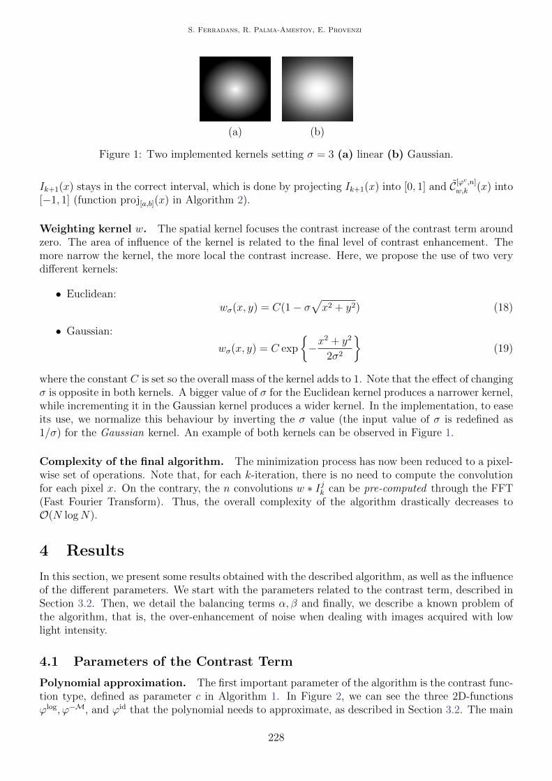
(a) (b)

Figure 1: Two implemented kernels setting σ = 3 (a) linear (b) Gaussian.

Ik+1(x) stays in the correct interval, which is done by projecting Ik+1(x) into [0, 1] and C[ϕc,n]w,k (x) into

[−1, 1] (function proj[a,b](x) in Algorithm 2).

Weighting kernel w. The spatial kernel focuses the contrast increase of the contrast term aroundzero. The area of influence of the kernel is related to the final level of contrast enhancement. Themore narrow the kernel, the more local the contrast increase. Here, we propose the use of two verydifferent kernels:

• Euclidean:wσ(x, y) = C(1− σ

√x2 + y2) (18)

• Gaussian:

wσ(x, y) = C exp

−x

2 + y2

2σ2

(19)

where the constant C is set so the overall mass of the kernel adds to 1. Note that the effect of changingσ is opposite in both kernels. A bigger value of σ for the Euclidean kernel produces a narrower kernel,while incrementing it in the Gaussian kernel produces a wider kernel. In the implementation, to easeits use, we normalize this behaviour by inverting the σ value (the input value of σ is redefined as1/σ) for the Gaussian kernel. An example of both kernels can be observed in Figure 1.

Complexity of the final algorithm. The minimization process has now been reduced to a pixel-wise set of operations. Note that, for each k-iteration, there is no need to compute the convolutionfor each pixel x. On the contrary, the n convolutions w ∗ Ijk can be pre-computed through the FFT(Fast Fourier Transform). Thus, the overall complexity of the algorithm drastically decreases toO(N logN).

4 Results

In this section, we present some results obtained with the described algorithm, as well as the influenceof the different parameters. We start with the parameters related to the contrast term, described inSection 3.2. Then, we detail the balancing terms α, β and finally, we describe a known problem ofthe algorithm, that is, the over-enhancement of noise when dealing with images acquired with lowlight intensity.

4.1 Parameters of the Contrast Term

Polynomial approximation. The first important parameter of the algorithm is the contrast func-tion type, defined as parameter c in Algorithm 1. In Figure 2, we can see the three 2D-functionsϕlog, ϕ−M, and ϕid that the polynomial needs to approximate, as described in Section 3.2. The main

228

An Algorithmic Analysis of Variational Models for Perceptual Local Contrast Enhancement

(a) (b) (c)

Figure 2: Surfaces obtained with Algorithm 1 for (a) c = log (b) c = −M (c) c = id.

difference between the functions relies in the extremes of the intensity range. In Figure 3 we showthe impact on the same images of changing the polynomial.

Weighting function diameter σ. The impact of the contrast term C[ϕc,n]w,k depends on the area

of influence of the kernel, which is defined by σ. As we increase σ, the contrast augments locally.Numerically, the values of σ are normalized to be adapted to the size of the input image. In Figure 4we can see the effect, on the output images, of changing the kernel w and the parameter σ. The firstrow corresponds to the original images, and the outputs are shown in the following rows.

On the first image set, we would like to point out how the algorithm is reproducing a well knownperceptual illusion known as “Mach bands” effect. In the original image, all bands are flat, but ourvisual system perceives them as having an “overshoot” to “undershoot” next to the intensity edges.This effect is reproduced by the output of the algorithm for σ = 1 for both kernels. This processimplies that our perception is changing the intrinsic geometry of the image, since it is introducingnew level lines. In fact, if we continue narrowing the kernel (σ = 3), the order of the level lines getsinverted, and the algorithm starts introducing an artifact called “sharpening”. This same behaviorcan be observed in a more subtle way on the results of the tree, specially on its leaves. The final setof images shows how the algorithm is able to discard a very strong color cast successfully with bothtypes of kernels, due to the independent application of the algorithm to each color channel.

4.2 Global Parameters: α, β

The parameters α, β balance the influence of the attachment to the mean value and original inputimage, respectively. The bigger the values the more influence their term has in the final output, ascan be observed in Figure 5. Note that for small values of α and β, the contrast term becomes moreimportant.

4.3 Possible Artifacts

This algorithm increases locally the contrast of an image. Intrinsically, this process can introducetwo types of artifacts:

229

S. Ferradans, R. Palma-Amestoy, E. Provenzi

(a) (b) (c)

Figure 3: Results obtained with the polynomials that approximate (a) c = log (b) c = −M (c)c = id. Note how the blue area of the book is rendered differently in the first set of images, as wellas the contrast on the leaves and clouds on the tree images.

• Noise enhancement: When applied to pictures taken under very dim conditions or with strongjpeg blocking, these artifacts can become visible, as can be observed on the first row of Figure 6.

• Sharpening: As explained previously, it consists in inverting the order of the level lines asshown in Figure 5 or Figure 6. This effect should not necessarily be considered as an artifact,but rather as the result of the deliberate application of an non-realistic style.

5 Conclusions

In this article, we have presented a thorough explanation and test of the algorithm presented in [7].This algorithm enhances contrast locally and improves the visibility of details in the input image.An interesting consequence of this process is that the global color cast produced by a colored light isremoved from the image. The algorithm is able to successfully do these tasks because it implementsseveral perceptual mechanisms developed by the human visual system: light adaptation, local con-trast enhancement and color constancy. Although the method relies on a set of parameters, whoseinfluence has been explored in this document, they can be set in a way that gives good results formost images.

Image Credits

Edoardo Provenzi, CC-BY-SA 3.0

Wiktionary (http://en.wiktionary.org/wiki/oak tree) CC-BY-SA 3.0

Kobus Barnard, SFU Computational Vision Laboratory3

Source image courtesy of albatros11, licensed by Getty images4

3http://www.cs.sfu.ca/~colour/data/4https://www.flickr.com/photos/albatros11/2509508972

230

An Algorithmic Analysis of Variational Models for Perceptual Local Contrast Enhancement

Ori

ginal

Eucl

idea

nG

auss

ian

Eucl

idea

nG

auss

ian

Eucl

idea

nG

auss

ian

σ = 0.1 σ = 1 σ = 2

Figure 4: Results obtained by setting c = log in Algorithm 1, and α = 1.1 and β = 1 in Algorithm 2.Note that the algorithm can produce an inversion of the level lines usually related to the sharpeningeffect, specially visible for σ = 2.

231

S. Ferradans, R. Palma-Amestoy, E. Provenzi

α = 1.1 α = 2 α = 3

β=

0.1

β=

0.5

β=

1β

=2

Figure 5: Changes in the output as α and β change. Note that for small values of α and β the strongterm is the contrast term C[ϕc,n]

w,k (x) in Equation (12). Increasing α ensures the global condition thatthe mean is close to µ. Increasing β forces the result to be closer to the original image, which in thiscase is dark and with a blue color cast. For all these results, c = id, σ = 1 and w is Gaussian.

(a) (b)

Figure 6: (a) Original image. (b) Result obtained with c = id, α = 1.1, β = 1, w is Gaussian andσ = 0.5 for the first row and σ = 3 for the second row. This in an example where the noise and thejpeg blocks are made visible, or a sharpening is produced after using the described algorithm.

232

An Algorithmic Analysis of Variational Models for Perceptual Local Contrast Enhancement

References

[1] L.A. Ambrosio, N. Gigli, and G. Savare, Gradient flows in metric spaces and in the spaceof probability measures, Lectures in Mathematics, Birkhauser, 2005.

[2] M. Bertalmıo, V. Caselles, and E. Provenzi, Issues about the retinex theory and contrastenhancement, International Journal of Computer Vision, (2009). http://dx.doi.org/10.1007/s11263-009-0221-5.

[3] M. Bertalmıo, V. Caselles, E. Provenzi, and A. Rizzi, Perceptual color correctionthrough variational techniques, IEEE Transactions on Image Processing, 16 (2007), pp. 1058–1072. http://dx.doi.org/10.1109/TIP.2007.891777.

[4] R.C. Gonzalez and R.E. Woods, Digital image processing, Prentice Hall, 2002.

[5] D.H. Hubel, Eye, Brain, and Vision, Scientific American Library, 1995.

[6] E.H. Land and J.J. McCann, Lightness and Retinex theory, Journal of the Optical Societyof America, 61 (1971), pp. 1–11.

[7] R. Palma-Amestoy, E. Provenzi, M. Bertalmıo, and V. Caselles, A perceptuallyinspired variational framework for color enhancement, IEEE Transactions on Pattern Analysisand Machine Intelligence, 31 (2009), pp. 458–474. http://dx.doi.org/10.1109/TPAMI.2008.86.

[8] E. Provenzi, L. De Carli, A. Rizzi, and D. Marini, Mathematical definition and analysisof the Retinex algorithm, Journal of the Optical Society of America A, 22 (2005), pp. 2613–2621.http://dx.doi.org/10.1364/JOSAA.22.002613.

[9] E. Provenzi, C. Gatta, M. Fierro, and A. Rizzi, Spatially variant white patch andgray world method for color image enhancement driven by local contrast, IEEE Transactions onPattern Analysis and Machine Intelligence, 30 (2008), pp. 1757–1770. http://dx.doi.org/10.1109/TPAMI.2007.70827.

[10] A. Rizzi, C. Gatta, and D. Marini, A new algorithm for unsupervised global and local colorcorrection, Pattern Recognition Letters, 24 (2003), pp. 1663–1677. http://dx.doi.org/10.

1016/S0167-8655(02)00323-9.

[11] G. Sapiro and V. Caselles, Histogram modification via differential equations, Journal ofDifferential Equations, 135 (1997), pp. 238–268. http://dx.doi.org/10.1006/jdeq.1996.

3237.

[12] R. Shapley and C. Enroth-Cugell, Visual adaptation and retinal gain controls, vol. 3,1984, pp. 263–346.

[13] G. Wyszecky and W. S. Stiles, Color science: Concepts and methods, quantitative dataand formulas, John Wiley & Sons, 2000.

233