An Algorithm for Network and Data-aware Placement of Multi-TierApplications in Cloud Data Centers

Md Hasanul Ferdausa,c,∗, Manzur Murshedb, Rodrigo N. Calheirosc, Rajkumar Buyyac

aFaculty of Information Technology, 25 Exhibition Walk, Clayton campus, Monash University, VIC 3800, AustraliabFaculty of Science and Technology, Federation University Australia, Northways Road, Churchill, VIC 3842, Australia

cCloud Computing and Distributed Systems (CLOUDS) Laboratory, Department of Computing and Information Systems, Building 168, TheUniversity of Melbourne, Parkville, VIC 3053, Australia

Abstract

Today’s Cloud applications are dominated by composite applications comprising multiple computing and data com-ponents with strong communication correlations among them. Although Cloud providers are deploying large numberof computing and storage devices to address the ever increasing demand for computing and storage resources, networkresource demands are emerging as one of the key areas of performance bottleneck. This paper addresses network-aware placement of virtual components (computing and data) of multi-tier applications in data centers and formallydefines the placement as an optimization problem. The simultaneous placement of Virtual Machines and data blocksaims at reducing the network overhead of the data center network infrastructure. A greedy heuristic is proposed forthe on-demand application components placement that localizes network traffic in the data center interconnect. Suchoptimization helps reducing communication overhead in upper layer network switches that will eventually reduce theoverall traffic volume across the data center. This, in turn, will help reducing packet transmission delay, increas-ing network performance, and minimizing the energy consumption of network components. Experimental resultsdemonstrate performance superiority of the proposed algorithm over other approaches where it outperforms the state-of-the-art network-aware application placement algorithm across all performance metrics by reducing the averagenetwork cost up to 67% and network usage at core switches up to 84%, as well as increasing the average number ofapplication deployments up to 18%.

Keywords: Virtual Machine, Network-aware, Storage, Data Center, Placement, Optimization, Cloud Application,Cloud Computing

1. Introduction

With the pragmatic realization of computing as a utility, Cloud Computing has recently emerged as a highly suc-cessful alternative information technology paradigm through the unique features of on-demand resource provisioning,pay-as-you-go business model, virtually unlimited amount of computing resources, and high reliability (Buyya et al.,2009). In order to meet the rapidly increasing demand for computing, communication, and storage resources, Cloudproviders are deploying large-scale data centers comprising thousands of servers across the planet. These data centersare experiencing sharp rise in network traffic and a major portion of this traffic is constituted of the data communica-tion within the data center. Recent report from Cisco Systems Inc. (Cisco, 2015) demonstrates that the Cloud datacenters will dominate the global data center traffic flow for the foreseeable future and its importance is highlighted byone of the top-line projections from this forecast that, by 2019, more than four-fifths of the total data center traffic willbe Cloud traffic (Figure 1). One important trait pointed out by the report is that a majority of the global data centertraffic is generated due to the data communication within the data centers: in 2014, it was 75.4% and it will be around73.1% in 2019.

∗Corresponding authorEmail addresses: md.ferdaus@monash.edu (Md Hasanul Ferdaus), manzur.murshed@federation.edu (Manzur Murshed),

rnc@unimelb.edu.au (Rodrigo N. Calheiros), rbuyya@unimelb.edu.au (Rajkumar Buyya)

Preprint submitted to Journal of Network and Computer Applications June 20, 2017

arX

iv:1

706.

0603

5v1

[cs

.DC

] 1

9 Ju

n 20

17

0.00

2.00

4.00

6.00

8.00

10.00

12.00

2014 2015 2016 2017 2018 2019

Traditional Data Center

Cloud Data Center

Zett

abyt

espe

r Yea

r

Year

61%

39%

83%

17%

Figure 1: Worldwide data center traffic growth (data source: Cisco).

This huge amount of intra-data center traffic is primarily generated by the application components that are cor-related to each other, for example, the computing components of a composite application (e.g., MapReduce) writingdata to the storage array after it has processed the data. This large growth of data center traffic may pose seriousscalability problems for wide adoption of Cloud Computing. Moreover, by the way of continuously rising popularityof social networking sites, e-commerce, and Internet-based gaming applications, large amount of data processing hasbecome an integral part of Cloud applications. Furthermore, scientific processing, multimedia rendering, workflow,and other massive parallel processing and business applications are being migrated to the Clouds due to the uniqueadvantages of high scalability, reliability, and pay-per-use business model. Over and above, recent trend in Big Datacomputing using Cloud resources (Assuncao et al., 2015) is emerging as a rapidly growing factor contributing to therise of network traffic in Cloud data centers.

One of the key technological elements that have paved the way for the extreme success of Cloud Computing isvirtualization. Modern data centers leverage various virtualization technologies (e.g., machine, network, and stor-age virtualization) to provide users an abstraction layer that delivers a uniform and seamless computing platform byhiding the underlying hardware heterogeneity, geographic boundaries, and internal management complexities (Zhanget al., 2010). By the use of virtualization, physical server resources are abstracted and shared through partial or fullmachine simulation by time-sharing, and hardware and software partitioning into multiple execution environments,known as Virtual Machines (VMs), each of which runs as a complete and isolated system. It allows dynamic sharingand reconfiguration of physical resources in Cloud infrastructures that make it possible to run multiple applicationsin separate VMs having different performance metrics. It also facilitates Cloud providers to improve utilization ofphysical servers through VM multiplexing (Meng et al., 2010a) and multi-tenancy, i.e., simultaneous sharing of phys-ical resources of the same server by multiple Cloud customers. Furthermore, it enables on-demand resource poolingthrough which computing (e.g., CPU and memory), network, and storage resources are provisioned to customers onlywhen needed (Kusic et al., 2009). By utilizing these flexible features of virtualization for provisioning physical re-sources, the scalability of data center network can be improved through minimization of network load imposed due tothe deployment of customer applications.

On the other side, modern Cloud applications are dominated by multi-component applications such as multi-tierapplications, massive parallel processing applications, scientific and business workflows, content delivery networks,and so on. These applications usually have multiple computing and associated data components. The computingcomponents are usually delivered to customers in the form of VMs, such as Amazon EC2 Instances1, whereas the data

1Amazon EC2 - Virtual Server Hosting, 2016. https://aws.amazon.com/ec2/

2

Web

Server

Application

Server

Data

Management

System

Data Blocks

Dispatcher/

Load Balancer

Presentation Tier Logic Tier Data Management Tier Storage Tier

Dispatcher/

Load Balancer

Figure 2: Multi-tier application architecture.

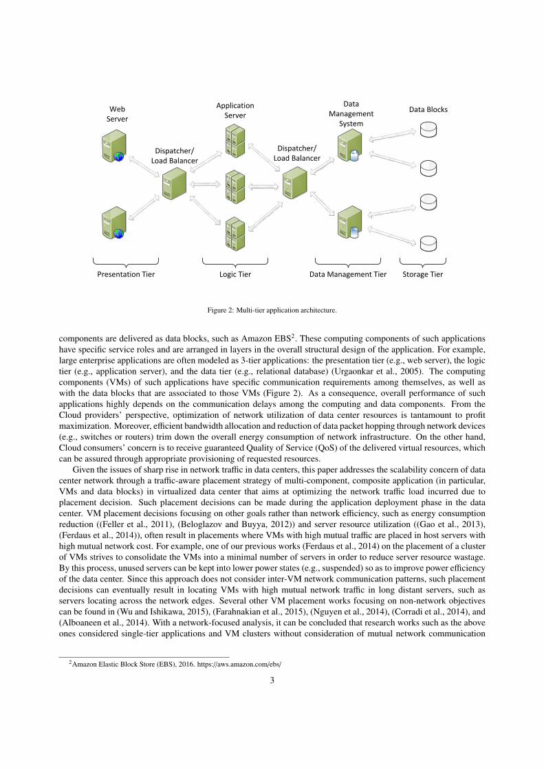
components are delivered as data blocks, such as Amazon EBS2. These computing components of such applicationshave specific service roles and are arranged in layers in the overall structural design of the application. For example,large enterprise applications are often modeled as 3-tier applications: the presentation tier (e.g., web server), the logictier (e.g., application server), and the data tier (e.g., relational database) (Urgaonkar et al., 2005). The computingcomponents (VMs) of such applications have specific communication requirements among themselves, as well aswith the data blocks that are associated to those VMs (Figure 2). As a consequence, overall performance of suchapplications highly depends on the communication delays among the computing and data components. From theCloud providers’ perspective, optimization of network utilization of data center resources is tantamount to profitmaximization. Moreover, efficient bandwidth allocation and reduction of data packet hopping through network devices(e.g., switches or routers) trim down the overall energy consumption of network infrastructure. On the other hand,Cloud consumers’ concern is to receive guaranteed Quality of Service (QoS) of the delivered virtual resources, whichcan be assured through appropriate provisioning of requested resources.

Given the issues of sharp rise in network traffic in data centers, this paper addresses the scalability concern of datacenter network through a traffic-aware placement strategy of multi-component, composite application (in particular,VMs and data blocks) in virtualized data center that aims at optimizing the network traffic load incurred due toplacement decision. Such placement decisions can be made during the application deployment phase in the datacenter. VM placement decisions focusing on other goals rather than network efficiency, such as energy consumptionreduction ((Feller et al., 2011), (Beloglazov and Buyya, 2012)) and server resource utilization ((Gao et al., 2013),(Ferdaus et al., 2014)), often result in placements where VMs with high mutual traffic are placed in host servers withhigh mutual network cost. For example, one of our previous works (Ferdaus et al., 2014) on the placement of a clusterof VMs strives to consolidate the VMs into a minimal number of servers in order to reduce server resource wastage.By this process, unused servers can be kept into lower power states (e.g., suspended) so as to improve power efficiencyof the data center. Since this approach does not consider inter-VM network communication patterns, such placementdecisions can eventually result in locating VMs with high mutual network traffic in long distant servers, such asservers locating across the network edges. Several other VM placement works focusing on non-network objectivescan be found in (Wu and Ishikawa, 2015), (Farahnakian et al., 2015), (Nguyen et al., 2014), (Corradi et al., 2014), and(Alboaneen et al., 2014). With a network-focused analysis, it can be concluded that research works such as the aboveones considered single-tier applications and VM clusters without consideration of mutual network communication

2Amazon Elastic Block Store (EBS), 2016. https://aws.amazon.com/ebs/

3

within the application components or VMs. On the contrary, this paper focuses on placing mutually communicatingcomponents of applications (such as VMs and data blocks) in data center components (such as physical serversand storage devices) with lesser network cost so that network overhead imposed due to the application placementis minimized. With this placement goal, the best placement for two communicating VMs would be in the sameserver where they can communicate through memory copy, rather than using the physical network links. This papereffectively addresses network-focused placement problem of multi-tiered applications with components having mutualnetwork communication rather than single-tiered ones. The significance of the network-focused placement of multi-tiered applications is evident from the experimental results presented later in Section 5, where it is observed that anefficient non-network greedy placement algorithm, namely First Fit Decreasing (FFD), incurs higher network costscompared to the proposed network-aware placement heuristic.

Moreover, advanced hardware devices with combined capabilities are opening new opportunities for efficient re-source allocation focusing on application needs. For example, Dell PowerEdge C8000 moduler servers are equippedwith CPU, GPU, and storage components that can work as multi-function devices. Combined placement of applicationcomponents with high mutual traffic (e.g., VMs and their associated data components) in such multi-function serverswill effectively reduce the data transfer delay since the data accessed by the VMs reside in the same devices. Similartrends are found in high-end network switches (e.g., Cisco MDS 9200 Multiservice Switches) that come with addi-tional built-in processing and storage capabilities. Reflecting on these technological development and multi-purposedevices, this paper has considered a generic approach in modeling computing, network, and storage elements in adata center so that placement algorithms can make efficient decision for application components placement in orderto achieve the ultimate goal of network cost reduction.

This research work investigates the allocation, specifically on-demand placement of composite application com-ponents (modeled as an Application Environment) requested by the customers to be deployed in Cloud data centerfocusing on network utilization, with consideration of computing, network, and storage resources capacity constraintsof the data center. In particular, this paper has the following contributions:

1. The Network-aware Application environment Placement Problem (NAPP) is formally defined as a combinato-rial optimization problem with the objective of network cost minimization due to the placement. The proposeddata center and application environment models are generic and are not restricted to any specific data centertopology and application type or structure, respectively.

2. Given the resource requirements and structure of the application environment to be deployed, and informationon the current resource state of the data center, a Network- and Data location-aware Application environmentPlacement (NDAP) scheme is proposed. NDAP is a greedy heuristic that generates mappings for simultaneousplacement of the computing and data components of the application into the computing and storage nodes of thedata center, respectively, focusing on minimization of incurred network traffic, while respecting the computing,network, and storage capacity constraints of data center resources. While making placement decisions, NDAPstrives to reduce the distance that data packets need to travel in the data center network, which in turn, helps tolocalize network traffic and reduces communication overhead in the upper layer network switches.

3. Finally, performance evaluation of the proposed approach is conducted through elaborate simulation-basedexperimentation across multiple performance metrics and several scaling factors. The results suggest that theNDAP algorithm successfully improves network resource utilization through efficient placement of applicationcomponents and outperforms compared algorithms significantly across all performance metrics.

The proposed NDAP greedy heuristic for placement of application environments, while optimizing the overallnetwork overhead, is addressing an important sub-problem of a much bigger multi-objective placement problem thatsimultaneously optimizes computing, storage, and communications resources. While many multi-objective works areavailable in the literature aiming at consolidation of the first two kinds of resources (computing and storage), worksaddressing all three kinds of resources are few and these works only considered placement of VMs in isolation. De-velopment of NDAP is the first step in addressing the comprehensive optimization problem considering the placementof a group of closely-linked VMs, hereby termed as an application environment.

The remainder of this paper is organized as follows. A brief background on the related works is presented inSection 2. Section 3 formally defines the addressed application placement problem (NAPP) as an optimization prob-lem, along with the associated mathematical models. The proposed network-aware, application placement approach

4

(NDAP) and its associated algorithms are elaborately explicated in Section 4. Section 5 details the experiments per-formed and shows the results, together with their analysis. Finally, Section 6 concludes the paper with a summary ofthe contribution and future research directions.

2. Related Work

During the past several years, a good amount of research works have been carried out in the area of VM scheduling,placement, and migration strategies in virtualized data centers, and more recently, focusing on Cloud data centers.A major portion of these works focus on servers resource utilization ((Nguyen et al., 2014), (Gao et al., 2013)),energy-efficiency ((Farahnakian et al., 2014), (Beloglazov, 2013)), and application performance ((Gupta et al., 2013),(Calcavecchia et al., 2012)), and so on (Ferdaus and Murshed, 2014) in the context of large infrastructures. Recently,a handful of works are published in the area of VM placement and migration with focus on network resources that arebriefly described below.

Kakadia et al. (2013) presented a VM grouping mechanism based on network traffic history within a data center atrun-time and proposed a fast, greedy VM consolidation algorithm in order to improve hosted applications performanceand optimize the network usage by saving internal bandwidth. Through simulation-based evaluation, the authors haveshown that the proposed VM consolidation algorithm achieves better performance compared to traditional VM place-ment approaches, within an order to magnitude faster and requires much less VM migrations. Dias and Costa (2012)addressed the problem of traffic concentration in data center networks by reallocating VMs in physical servers basedon current traffic matrix and server resource usage. The authors proposed a scheme for partitioning server basedon connectivity capacity and available computing resources, as well as VM clustering mechanism depending on theamount of data exchanged among the VMs. The proposed VM placement algorithm tries to find mappings for match-ing all the VM clusters in the server partitions, respecting the server resource capacity constraints. Shrivastava et al.(2011) proposed a topology-aware VM migration scheme for managing overloaded VMs considering the completeapplication context running on the VMs and the server resource capacity constraints. The goal of the proposed VMmigration algorithm is to relocate overloaded VMs to physical servers so that the run-time network load within datacenter is minimized. Similar VM placement and relocation works can be found in (Zhang et al., 2016), (Biran et al.,2012), and (Meng et al., 2010b), demand-based VM provisioning works for multi-component Cloud applications arepresented in (Srirama and Ostovar, 2014) and in (Sahu et al., 2014). All the above mentioned traffic-aware VM place-ment and consolidation works aim at run-time scenarios for relocating running VMs within the data center throughVM migration.

Several other recent VM placement and consolidation works have been proposed focusing on simultaneous op-timization of energy and traffic load in data centers. Vu and Hwang (2014) addressed the issues of VM migrationfrom underloaded and overloaded PMs at run-time and presented an offline algorithm for individual VM migrationwith the focus on traffic- and energy consumption reduction. Energy efficiency is achieved by consolidating VMs inhigh capacity servers as much as possible and traffic efficiency is achieved by migrating VMs near to communicatingpeer VMs. Wang et al. (2014) addressed the problem of unbalanced resource utilization and network traffic in datacenter during run-time, and proposed an energy-efficient and QoS-aware VM placement mechanism that groups therunning VMs into partitions to reduce traffic communication across the data center, determines to server for migratingthe VMs, and finally, uses the OpenFlow controller to assign paths to balance the traffic load and avoid congestion.Takouna et al. (2013) presented mechanisms for dynamically determining the bandwidth demand and communica-tion patter of HPC and parallel applications in data center and reallocating the communicative VMs through livemigration. The objective of the proposed approach is to reduce network link utilization and energy saving throughaggregating communicative VMs. The authors have shown substantial improvement in data center traffic volumethrough simulation-based evaluation. Gao et al. (2016) addressed the problem of energy cost reduction under bothserver and network resource constraints within data center and proposed a VM placement strategy based on AntColony Optimization incorporating network resource factor with server resources.

Huang et al. (2013) addressed the server overload problem and presented a three-stage joint optimization frame-work that minimizes the number of used servers in the data center in order to reduce power consumption, communi-cation costs, and finally, a combined approach that focus on both the above goals through the use of VM migrations.Lloyd et al. (2014) investigated the problem of virtual resource provisioning and placement of service oriented appli-cations through dynamic scaling in Cloud infrastructures and presented a server load-aware VM placement scheme

5

that improves application performance and reduces resource cost. Similar multi-objective VM placement and migra-tion works can also be found in (Zhang et al., 2012), (Huang et al., 2012), (Wang et al., 2013), and (Song et al., 2012)that target optimization of energy consumption reduction, server resource utilization, and network usage. Given thefact that VM live migrations are costly operations (Liu et al., 2013), the above mentioned VM relocation strategiesoverlook the impact of necessary VM migrations and reconfiguration on hosted applications, physical servers andnetwork devices. Further recent works on network-aware VM placement and migration can be found in (Li and Qian,2015), (Alharbi and Walker, 2016), (Cui et al., 2017), (Zhao et al., 2015), and (Wang et al., 2016). A detailed tax-onomy and survey on various existing network-aware VM management strategies can be found in our previous work(Ferdaus et al., 2015).

Contrary to the above mentioned works, this paper addresses the problem of network efficient, on-demand place-ment of composite applications consisting of multiple VMs and associated data components, along with inter-componentcommunication pattern, in a data center consisting of both computing servers and storage devices. The addressedproblem does not involve VM migrations since the placement decision is taken during the application deploymentphase. Recently, Georgiou et al. (2013) have addressed the benefit of user-provided hints on inter-VM communicationduring the online VM cluster placement and proposed two placement heuristics utilizing the properties of PortLandnetwork topology (Mysore et al., 2009). However, this work does not involve any data component for VM-clusterspecification. On the other hand, both of the proposed composite, multi-tier application and data center models ofthis paper are generic and are not restricted to any particular application or data center topology. Data location-awareVM placement works can be found in (Piao and Yan, 2010) and in (Korupolu et al., 2009); however, these worksmodeled the applications as single instance of VM, which is an oversimplified view of today’s Cloud or Internetapplications that are mostly composed of multiple computing and storage entities in multi-tier structure with strongcommunication correlations among the components. In order to reflect on this, this paper investigates a much widerVM communication model by considering placement of Application Environments, each involving a number of VMsand associated data blocks with sparse communication links between them.

3. Problem Statement

While deploying composite applications in Cloud data centers, such as multi-tier or workflow applications, cus-tomers request multiple computing VMs in the form of a VM cluster or a Virtual Private Cloud and multiple DataBlocks (DBs). These computing VMs have specific traffic flow requirements among themselves, as well as with thedata blocks. The remainder of this section formally defines such composite application environment placement as anoptimization problem. Figure 3 presents a visual representation of the application placement in data center and Table1 provides the various notations used in the problem definition and proposed solution.

3.1. Formal DefinitionAn Application Environment is defined as AE = {V MS ,DBS }, where VMS is the set of requested VMs: V MS =

{V Mi : 1 ≤ i ≤ Nv} and DBS is the set of requested DBs: DBS = {DBk : 1 ≤ k ≤ Nd}. Each VM V Mi has specificationof its CPU and memory demands represented by V Mcpu

i and V Mmemi , respectively, and each DB DBk has specification

of its storage resource demand denoted by DBstrk .

Data communication requirements between any two VMs, and between a VM and a DB are specified as VirtualLinks (VLs) between 〈V M,V M〉 pairs and 〈V M,DB〉 pairs, respectively, during AE specification and deployment. Thebandwidth demand or traffic load between V Mi and V M j is represented by BW(V Mi,V M j). Similarly, the bandwidthdemand between V Mi and DBk is represented by BW(V Mi,DBk). These bandwidth requirements are provided as userinput along with the VM and DB specifications.

A Data Center is defined as DC = {CNS , S NS } where CNS is the set of computing nodes (e.g., physical serversor computing components of a multi-function storage device) in DC: CNS = {CNp : 1 ≤ p ≤ Nc} and SNS is the set ofstorage nodes: S NS = {S Nr : 1 ≤ r ≤ Ns}. For each computing node CNp, the available CPU and memory resourcecapacities are represented by CNcpu

p and CNmemp , respectively. Here available resources mean the remaining usable

resources of a CN that may have already hosted other VMs that are consuming the rest of the resources. Similarly, foreach storage node S Nr, the available storage resource capacity is represented by S N str

r .Computing nodes and storage nodes are interconnected through Physical Links (PLs) in the data center commu-

nication network. PL distance and available bandwidth between two computing nodes CNp and CNq are denoted by

6

VMj DBkVL VMi

Virtual Machines Data Blocks

BW(VMi, VMj)VL

SNrCNp

CNq

BA(CNp, CNq)

BW(VMi, DBk)

Compute Nodes Storage Nodes

DS(CNp, CNq)

BA(CNp, SNr)

DS(CNp, SNr)

Figure 3: Application environment placement on data center.

DS (CNp,CNq) and BA(CNp,CNq), respectively. Similarly, PL distance and available bandwidth between a comput-ing node CNp and a storage node S Nr are represented by DS (CNp, S Nr) and BA(CNp, S Nr), respectively. PL distancecan be any practical measure, such as link latency, number of hops or switches, and so on. Also, the proposed modeldoes not restrict the data center to a fixed network topology. Thus, the network distance DS and available bandwidthBA models are generic and different model formulations focusing on any particular network topology or architecturecan be readily applied in the optimization framework and proposed solution. In the experiments, the number of hopsor switches between any two data center nodes is used as the only input parameter for DS function in order to mea-sure the PL distance. Although singular distances between 〈CN,CN〉 and 〈CN, S N〉 pairs are used in the experiments,network link redundancy and multiple communication paths in data center can be incorporated in the proposed modeland placement algorithm by appropriately defining distance function (DS ) and available bandwidth function (BA),respectively.

Furthermore, DN(V Mi) denotes the computing node where V Mi is currently placed, otherwise if V Mi is notalready placed, DN(V Mi) = null. Similarly, DN(DBk) denotes the storage node where DBk is currently placed.

The network cost of placing V Mi in CNp and V M j in CNq is defined as the following:

Cost(V Mi,CNp,V M j,CNq) = BW(V Mi,V M j) × DS (CNp,CNq). (1)

Likewise, the network cost of placing V Mi in CNp and DBk in S Nr is defined as the following:

Cost(V Mi,CNp,DBk, S Nr) = BW(V Mi,DBk) × DS (CNp, S Nr). (2)

Given the AE to deploy in the DC, the objective of the NAPP problem is to find placements for VMs and DBsin CNs and SNs, respectively, in such a way that the overall network cost or communication overhead due to the AEdeployment is minimized. Thus, the Objective Function f is defined as the following:

7

Table 1: Notations and their meaningsNotation Meaning

V M Virtual MachineDB Data BlockAN AE node (either a VM or a DB)V MS Set of VMs in an AEDBS Set of DBs in an AEANS Set of ANs (ANS = {V MS ∪ DBS }) in an AENv Total number of VMs in an AENd Total number of DBs in an AEVL Virtual LinkVCL Virtual Computing Link that connects two VMsVDL Virtual Data Link that connects a VM and a DBvclList Ordered list of VCLs in an AEvdlList Ordered list of VDLs in an AENvc Total number of VCLs in an AENvd Total number of VDLs in an AENvn Average number of NTPP VLs of a VM or a DBBW(V Mi,V M j) Bandwidth demand between V Mi and V M j

BW(V Mi,DBk) Bandwidth demand between V Mi and DBk

CN Computing NodeS N Storage NodeDN(AN) DC node where AN is placedCNS Set of CNs in a DCS NS Set of SNs in a DCNc Total number of CNs in a DCNs Total number of SNs in a DCcnList Ordered list of CNs in a DCsnList Ordered list of SNs in a DCPL Physical network LinkPCL Physical Computing Link that connects two CNsPDL Physical Data Link that connects a CN and a SNDS (CNp,CNq) Network distance between CNp and CNq

DS (CNp, S Nr) Network distance between CNp and S Nr

BA(CNp,CNq) Available bandwidth between CNp and CNq

BA(CNp, S Nr) Available bandwidth between CNp and S Nr

minimize∀i:DN(V Mi)∀k:DN(V Mk)

f (AE,DC) =

Nv∑i=1

( Nv∑j=1

Cost(V Mi,DN(V Mi),V M j,DN(V M j))+

Nd∑k=1

Cost(V Mi,DN(V Mi),DBk,DN(DBk))).

(3)

The above AE placement is subject to the constraints that the available resource capacities of any CN and SN arenot violated:

∀p :∑

∀i:DN(V Mi)=CNp

V Mcpui ≤ CNcpu

p . (4)

8

∀p :∑

∀i:DN(V Mi)=CNp

V Mmemi ≤ CNmem

p . (5)

∀r :∑

∀k:DN(DBk)=S Nr

DBstrk ≤ S N str

r . (6)

Furthermore, the sum of the bandwidth demands of the VLs that are placed on each PL must be less or equal tothe available bandwidth of the PL:

∀p∀q : BA(CNp,CNq) ≥∑

∀i:DN(V Mi)=CNp

∑∀ j:DN(V M j)=CNq

BW(V Mi,V M j). (7)

∀p∀r : BA(CNp, S Nr) ≥∑

∀i:DN(V Mi)=CNp

∑∀k:DN(DBk)=S Nr

BW(V Mi,DBk). (8)

Given that every VM and DB placement fulfills the above mentioned constraints (Eq. 4–8), the NAPP problemdefined by objective function f (Eq. 3) is explained as: among all possible feasible placements of VMs and DBs inAE, the placement that has minimum cost is the optimal solution. Thus, NAPP falls in the category of combinatorialoptimization problem. In particular, it is an extended form of the Quadratic Assignment Problem (QAP) (Loiola et al.,2007), which is proven to be computationally NP−hard (Burkard et al., 1998).

4. Proposed Solution

The proposed network-aware VM and DB placement approach (NDAP) tries to place the VLs in such a way thatnetwork packets need to travel short distances. For better explanation of the solution approach, the above describedmodels of AE and DC are extended by adding few other notations.

Every AE node is represented by AN which can either be a VM or a DB, and the set of all ANs in an AE isrepresented by ANS . Every VL can be either a Virtual computing Link (VCL), i.e., VL between two VMs or a VirtualData Link (VDL), i.e., VL between a VM and a DB. The total number of VCL and VDL in an AE is represented by Nvc

and Nvd, respectively. All the VCLs and VDLs are maintained in two ordered lists vclList and vdlList, respectively.While VM-VM communication (VCL) and VM-DB communication (VDL) may be considered closely related, theydiffer in terms of actor and size. As only a VM can initiate communications, VCL supports an ”active” duplex linkwhile VDL supports a ”passive” duplex link. More distinctly, bandwidth demands of VDLs are multiple orders largerthan the same of VCLs.

Every DC node is represented by DN which can either be a CN or a S N. All the CNs and SNs in a DC aremaintained in two ordered lists cnList and snList, respectively. Every PL can be either a Physical computing Link(PCL), i.e., PL between two CNs or a Physical Data Link (PDL) i.e., PL between a CN and a SN.

The proposed NDAP algorithm is a greedy heuristic that first sorts the vdlList and vclList in decreasing orderof the bandwidth demand of VDLs and VCLs. Then, it tries to places all the VDLs from vdlList, along with anyassociated VCLs to fulfill placement dependency, on the feasible PDLs and PCLs, and their associated VMs and DBsin CNs and SNs, respectively, focusing on the goal of minimizing the incurred network cost due to placement of allthe VDLs and associated VCLs. Finally, NDAP tries to place the remaining VCLs from vclList on PCLs, along withtheir associated VMs and DBs in CNs and SNs, respectively, again targeting on reducing the incurred network cost.

As mentioned in Section 3, NAPP is in fact an NP−hard combinatorial optimization problem similar to QAPand Sahni and Gonzalez (1976) have shown that even finding an approximate solution for QAP within some constantfactor from the optimal solution cannot be done in polynomial time unless P = NP. Considering the fact that greedyheuristics are relatively fast, easy to understand and implement, and very often used as an effective solution approachfor NP−complete problems, this paper proposes NDAP greedy heuristic as a solution for the NAPP problem.

9

A straight forward placement of an individual VL (either VDL or VCL) on a preferred PL is not always possiblesince one or both of its ANs can have Peer ANs connected by Peer VLs (Figure 4(a)). At any point during an AEplacement process, a VL can have Peer ANs that are already placed. The peer VLs that have already-placed peerANs is termed as need-to-place peer VLs (NTPP VLs), indicating the condition that placement of any VL also needsto perform simultaneous placement of its NTPP VLs, and the average number of NTPP VLs for any VM or DB isdenoted by Nvn. The maximum value of Nvn can be Nv + Nd − 1 which indicates that the corresponding VM or DBhas VLs with all the other VMs and DBs in the AE. Since, for any VL placement, the corresponding placement of itsNTPP VLs is an integrated part of the NDAP placement strategy, firstly the VL placement feasibility part of the NDAPalgorithm is presented in the following subsection. Afterwards, the next four subsections describe other constituentcomponents of the NDAP algorithm. Finally, a detailed description of the final NDAP algorithm is provided alongwith the pseudocode.

4.1. VL Placement FeasibilityDuring the course of AE placement, when NDAP tries to place a VL that has one or both of its ANs not placed

yet (i.e., DN(AN) = null), then a feasible placement for the VL needs to ensure that (1) the VL itself is placed on afeasible PL, (2) its ANs are placed on feasible DNs, and (3) all the NTPP VLs are placed on feasible PLs.

Depending on the type of VL and the current placement status of its ANs, five different cases may arise that arepresented below. The NDAP placement algorithm handles these five cases separately. Figure 4(b)-(f) provide a visualrepresentation of the five cases where the VL to place is shown as solid green line and its NTPP VLs are shown assolid blue lines.

VDL Placement: When trying to place a VDL, any of the following three cases may arise:Case 1.1: Both the V M and DB are not placed yet and their peers V M1, DB1, and V M2 are already placed (Figure

4(b)).Case 1.2: DB is placed but V M is not placed yet and V M’s peers V M1 and DB1 are already placed (Figure 4(c)).Case 1.3: V M is placed but DB is not placed yet and DB’s peer V M1 is already placed (Figure 4(d)).VCL Placement: In case of VCL placement, any of the following two cases may arise:Case 2.1: Both the VMs (V M1 and V M2) are not placed yet and their peers V M3, DB1, V M4, and DB2 are already

placed (Figure 4(e)).Case 2.2: Only one of the VMs is already placed and its peers V M3 and DB1 are already placed (Figure 4(f)).In all the above cases, placement feasibility of the NTPP VDLs and VCLs of the not-yet-placed VMs and DBs

must be checked against the corresponding PDLs and PCLs, respectively (Eq. 7 & 8).

4.2. Feasibility and Network Cost of VM and Peer VLs PlacementWhen NDAP tries to place a VM in a CN, it is feasible when (1) the computing and memory resource demands of

the VM can be fulfilled by the remaining computing and memory resource capacities of the CN, and (2) the bandwidthdemands of all the NTPP VLs can be satisfied by the available bandwidth capacities of the corresponding underlyingPLs (Figure 5(a)):

V MPeerFeas(V M,CN) =

1, if Eq. 4 & 5 holds and, DN(AN) , null and

BW(V M, AN) ≤ BA(CN,DN(AN)) for ∀AN;0, otherwise.

(9)

When NDAP tries to place two VMs (V M1 and V M2) in a single CN, it is feasible when (1) the combinedcomputing and memory resource demands of the two VMs can be fulfilled by the remaining computing and memoryresource capacities of the CN, and (2) the bandwidth demands of all the NTPP VLs of both the VMs can be satisfiedby the available bandwidth capacities of the corresponding underlying PLs:

V MPeerFeas(V M1,V M2,CN) =

1, if Eq. 4 & 5 holds for (V M1 + V M2) and,∀AN : DN(AN) , null and,BW(V M1, AN) + BW(V M2, AN) ≤ BA(CN,DN(AN));

0, otherwise.

(10)

10

VM

Already-placed Peer VM

DB

NTPP VL

Not-yet-placed Peer VM

Peer VL

Not-yet-placed Peer DB

NTPP VL

Already-placed Peer DB

Peer VL

VM1

VMDB

DB1

VM2

VM1

VMDB

DB1

(a) (b) (c)

VDL

VDL

VM3

VM1

DB2

DB1

VM4

(d) (e) (f)

VCL

VM1

VMDBVDL

VM2

VM3

VM1

DB1

VCL

VM2

Already-placed VM Already-placed DB Compute Node Storage Node

Case 1.1 Case 1.2

Case 1.3 Case 2.1 Case 2.2

Not-yet-placed VM Not-yet-placed DB VM to place DB to place

Figure 4: (a) Peer VL and NTPP VL, and (b-f) Five possible VL placement scenarios.

The network cost of a VM placement is measured as the accumulated cost of placing all of its NTPP VLs:

V MPeerCost(V M,CN) =∑

∀AN: DN(AN),null∧BW(V M,AN)>0

Cost(V M,CN, AN,DN(AN)). (11)

4.3. Feasibility and Network Cost of DB and Peer VLs Placement

When trying to place a DB in a SN, it is feasible when (1) the storage resource demand of the DB can be fulfilled bythe remaining storage resource capacity of the SN, and (2) the bandwidth demands of the NTPP VLs can be satisfiedby the available bandwidth capacities of corresponding underlying PLs (Figure 5(a)):

DBPeerFeas(DB, S N) =

1, if Eq. 6 holds and, DN(AN) , null and

BW(AN,DB) ≤ BA(DN(AN), S N) for ∀AN;0, otherwise.

(12)

The network cost of any DB placement is measured as the total cost of placing all of its NTPP VLs:

DBPeerCost(DB, S N) =∑

∀AN: DN(AN),null∧BW(AN,DB)>0

Cost(AN,DN(AN),DB, S N). (13)

11

SNCN

VM DBVDL

NTPP VL

(a)

SN

CN2

VCL

NTPP VL

(b)

PDL

CN1

VM1 VM2

PCL

PDL

PCL

NTPP VL

NTPP VL

Figure 5: Placement of (a) VDL and (b) VCL along with NTPP VLs.

4.4. VM and Peer VLs Placement

Algorithm 1 shows the subroutine for placing a V M and its associated NTPP VLs. Firstly, the V M-to-CN place-ment is accomplished by reducing the available CPU and memory resource capacities of the CN by the amount ofCPU and memory resource requirements of the V M and setting the CN as the DC node of the V M [line 1]. Then,for each already-placed peer AN of V M (i.e., any AN that has non-zero traffic load with V M and DN(AN) , null),it is checked if the selected CN is different from the computing node where the peer AN is placed, in which case theavailable bandwidth capacity of the PL that connects the selected CN and DN(AN) is reduced by the amount of thebandwidth demand of the corresponding NTPP VL [lines 2–4]. In those cases where the selected CN is the com-puting node where the peer AN is placed, the V M can communicate with the peer AN through memory copy insteadof passing packet through physical network links. Afterwards, the NTPP VL is removed from the vclList or vdlList,depending on whether it is a VCL or VDL, respectively, in order to indicate that it is now placed [lines 5–7].

4.5. DB and Peer VLs Placement

Algorithm 2 shows the subroutine for placing a DB in a S N and its associated NTPP VLs. Firstly, the DB-to-S Nplacement is performed by reducing the available storage capacity of the S N by the amount of the storage requirementsof the DB and by setting the S N as the DC node of DB [line 1]. Then, for every already-placed peer AN of DB (i.e.,any AN that has non-zero traffic load with DB and DN(AN) , null), the available bandwidth capacity of the PDL thatconnects the selected S N and DN(AN) is reduced by the amount of the NTPP VL’s bandwidth requirement and theNTPP VL is removed from the vdlList to mark that it is now placed [lines 2–6].

12

Algorithm 1 PlaceVMandPeerVLsInput: V M to place, CN where V M is being placed, set of all ANs ANS , vclList, and vdlList.Output: V M-to-CN and VL-to-PL placements.

1: CNcpu ← CNcpu − V Mcpu; CNmem ← CNmem − V Mmem; DN(V M)← CN;2: for each AN ∈ ANS do3: if BW(V M, AN) > 0 ∧ DN(AN) , null then4: if DN(AN) , CN then BA(CN,DN(AN))← BA(CN,DN(AN)) − BW(V M, AN); endif5: VL← virtualLink(V M, AN);6: if VL is a VCL then vclList.remove(VL);7: else vdlList.remove(VL);8: endif9: end if

10: end for

Algorithm 2 PlaceDBandPeerVLsInput: DB to place, S N where DB is being placed, set of all ANs ANS , and vdlList.Output: DB-to-S N and VL-to-PL placements.

1: S N str ← S N str − DBstr; DN(DB)← S N;2: for each AN ∈ ANS do3: if BW(AN,DB) > 0 ∧ DN(AN) , null then4: BA(DN(AN), S N)← BA(DN(AN), S N) − BW(AN,DB); VL← virtualLink(AN,DB); vdlList.remove(VL);5: end if6: end for

4.6. NDAP Algorithm

The pseudocode of the final NDAP algorithm is presented in Algorithm 3. It receives the DC and AE as inputand returns the network cost incurred due to the AE placement. NDAP begins by performing necessary initializationand sorting the vdlList and vclList in decreasing order of their VLs’ bandwidth demands [line 1]. Afterwards, ititeratively takes the first VDL from vdlList (i.e., VDL with highest bandwidth demand) and tries to place it (alongwith its VM and DB, and all NTPP VLs) in a PDL among the feasible PDLs so that the total network cost incurreddue to the placement is minimum [lines 2–29] (Figure 5(a)). As explained in Section 4.1, there can be three cases forthis placement depending on current placement status of the VDL’s VM and DB.

When the VDL matches Case 1.1 (both VM and DB are not placed), then for each feasible CN and SN in DC(Eq. 9 and 12), it is checked if the bandwidth demand of the VDL can be satisfied by the available bandwidth of thecorresponding PDL connecting the CN and SN. If it can be satisfied, then the total cost of placing the VDL and itsassociated NTPP VLs is measured (Eq. 11 and 13). The 〈CN, S N〉 pair that offers the minimum cost is selected forplacing the 〈V M,DB〉 pair and the available bandwidth capacity of the PDL that connects the selected 〈CN, S N〉 pairis updated to reflect the VDL placement [lines 4–13]. When the VDL matches Case 1.2 (VM is not placed, but DBis placed), the feasible CN that offers minimum cost placement is selected for the VM and the total cost is measured[lines 14–18]. In a similar way, Case 1.3 (VM is placed, but DB is not placed) is handled in lines 19–24 and the bestSN is selected for the DB placement.

If NDAP fails to find a feasible CN or SN, it returns −1 to indicate failure in finding a feasible placement for the AE[line 25]. Otherwise, it activates the placements of the VM and DB along with their NTPP VLs by using subroutinesPlaceV MandPeerVLs (Algorithm 1) and PlaceDBandPeerVLs (Algorithm 2), accumulates the measured cost invariable totCost, and removes the VDL from vdlList [lines 26–28]. In this way, by picking the VDLs from a list thatis already sorted based on bandwidth demand and trying to place each VDL, along with its NTPP VLs, in such a waythat the incurred network cost is minimum in the current context of the DC resource state, NDAP strives to minimizethe total network cost of placing the AE as formulated by the objective function f (Eq. 3) of the proposed optimization.In particular, in each iteration of the first while loop (lines 2–29), NDAP pick the next highest bandwidth demandingVDL from the vdlList and finds the best placement (i.e., minimum cost) for it along with its NTPP VLs. Moreover, the

13

Algorithm 3 NDAP AlgorithmInput: DC and AE.Output: Total network cost of AE placement.1: totCost ← 0; Sort vdlList and vclList in decreasing order of VL’s bandwidth demands;2: while vdlList , ∅ do {NDAP tries to place all VDLs in vdlList}3: VDL← vdlList[0]; minCost ← ∞; V M ← VDL.V M; DB← VDL.DB; selCN ← null; selS N ← null;4: if DN(V M) = null ∧ DN(DB) = null then {Case 1.1: Both VM and DB are not placed}5: for each CN ∈ cnList ∧ V MPeerFeas(V M,CN) = 1 do6: for each S N ∈ snList ∧ DBPeerFeas(DB, S N) = 1 do7: if BW(V M,DB) ≤ BA(CN, S N) then8: cost ← BW(V M,DB) × DS (CN, S N) + V MPeerCost(V M,CN) + DBPeerCost(DB, S N);9: if cost < minCost then minCost ← cost; selCN ← CN; selS N ← S N; endif

10: end if11: end for12: end for13: if minCost , ∞ then BA(selCN, selS N)← BA(selCN, selS N) − BW(V M,DB); endif14: else if DN(V M) = null ∧ DN(DB) , null then {Case 1.2: VM is not placed and DB is already placed}15: for each CN ∈ cnList ∧ V MPeerFeas(V M,CN) = 1 do16: cost ← V MPeerCost(V M,CN);17: if cost < minCost then minCost ← cost; selCN ← CN; endif18: end for19: else if DN(V M) , null ∧ DN(DB) = null then {Case 1.3: VM is already placed and DB is not placed}20: for each S N ∈ snList ∧ DBPeerFeas(DB, S N) = 1 do21: cost ← DBPeerCost(DB, S N);22: if cost < minCost then minCost ← cost; selS N ← S N; endif23: end for24: end if25: if minCost = ∞ then return −1; endif {Feasible placement not found}26: if selCN , null then PlaceV MandPeerVLs(V M, selCN); endif {For Case 1.1 and Case 1.2}27: if selS N , null then PlaceDBandPeerVLs(DB, selS N); endif {For Case 1.1 and Case 1.3}28: totCost ← totCost + minCost; vdlList.remove(0);29: end while30: while vclList , ∅ do {NDAP tries to place remaining VCLs in vclList}31: VCL← vclList[0]; minCost ← ∞; V M1 ← VCL.V M1; V M2 ← VCL.V M2; selCN1 ← null; selCN2 ← null;32: if DN(V M1) = null ∧ DN(V M2) = null then {Case 2.1: Both VMs are not placed}33: for each CN1 ∈ cnList ∧ V MPeerFeas(V M1,CN1) = 1 do34: for each CN2 ∈ cnList ∧ V MPeerFeas(V M2,CN2) = 1 do35: if CN1 = CN2 ∧ V MPeerFeas(V M1,V M2,CN) = 0 then continue; endif36: if BW(V M1,V M2) ≤ BA(CN1,CN2) then37: cost ← BW(V M1,V M2) × DS (CN1,CN2);38: cost ← cost + V MPeerCost(V M1,CN1) + V MPeerCost(V M2,CN2);39: if cost < minCost then minCost ← cost; selCN1 ← CN1; selCN2 ← CN2; endif40: end if41: end for42: end for43: if minCost , ∞ then BA(selCN1, selCN2)← BA(selCN1, selCN2) − BW(V M1,V M2); endif44: else if DN(V M1) , null ∨ DN(V M2) , null then {Case 2.2: One of the VMs is not placed}45: if DN(V M1) , null then swap values of V M1 and V M2; endif {Now V M1 denotes the not-yet-placed VM}46: for each CN1 ∈ cnList ∧ V MPeerFeas(V M1,CN1) = 1 do47: cost ← V MPeerCost(V M1,CN1);48: if cost < minCost then minCost ← cost; selCN1 ← CN1; endif49: end for50: end if51: if minCost = ∞ then return −1; endif {Feasible placement not found}52: PlaceV MandPeerVLs(V M1, selCN1); {For Case 2.1 and Case 2.2}53: if selCN2 , null then PlaceV MandPeerVLs(V M2, selCN2); endif {For Case 2.1}54: totCost ← totCost + minCost; vclList.remove(0);55: end while56: return totCost;

placement of the VDLs are performed before the placement of the VCLs since the average VDL bandwidth demandis expected to be higher than the average VCL bandwidth demand considering the fact that the average traffic volumefor 〈V M,DB〉 pair is supposed to be higher than that for 〈V M,V M〉 pair.

After NDAP has successfully placed all the VDLs, then it starts placing the remaining VCLs in the vclList (i.e.,VCLs that were not NTPP VLs during the VDLs placement). For this part of the placement, NDAP applies a similarapproach by repeatedly taking the first VCL from vclList and trying to place it on a feasible PCL so that the incurrednetwork cost is minimum [lines 30–55] (Figure 5(b)). This time, there can be two cases depending on the placementstatus of the two VMs of the VCL (Section 4.1).

When the VCL matches Case 2.1 (both VMs are not placed), then for each feasible CN in DC (Eq. 9), it isfirst checked if both the VMs (V M1 and V M2) are being tried for placement in the same CN. In such cases, if the

14

combined placement of both the VMs along with their NTPP VLs are not feasible (Eq. 10), then NDAP continueschecking feasibility for different CNs [line 35]. When both VMs placement feasibility passes and the bandwidthdemand of the VCL can be satisfied by the available bandwidth of the corresponding PCL connecting the CNs, thenthe total cost of placing the VCL and its associated NTPP VLs is measured (Eq. 11 and 13) [lines 36–40]. Whenboth the VMs are being tried for the same CN, then they can communicate with each other using memory copy rathergoing through physical network link and the available bandwidth check in line 36 works correctly since the intra-CNavailable bandwidth is considered to be unlimited. The 〈CN1,CN2〉 pair that offers the minimum cost is selected forplacing the 〈V M1,V M2〉 pair and the available bandwidth capacity of the PCL connecting the selected 〈CN1,CN2〉

pair is updated to reflect the VCL placement [lines 39–43]. When the VCL matches Case 2.2 (one of the VMs is notplaced), the feasible CN that offers minimum cost placement is selected for the not-yet-placed VM (V M1) and thetotal cost is measured [lines 44–50].

Similar to VDL placement, if NDAP fails to find feasible CNs for any VCL placement, it returns −1 to indicatefailure [line 51]. Otherwise, it activates the placements of the VMs along with their NTPP VLs by using subroutinePlaceV MandPeerVLs (Algorithm 1), accumulates the measured cost in totCost, and removes the VCL from vclList[lines 52–55]. For the same reason as for VDL placement, the VCL placement part of the NDAP algorithm fostersthe reduction of the objective function f value (Eq. 3).

Finally, NDAP returns the total cost of the AE placement, which also indicates a successful placement [line 56].

5. Performance Evaluation

This section describes the performance of the proposed NDAP algorithm compared to other algorithms througha set of simulation based experiments. Section 5.1 gives a brief description of the evaluated algorithms, Section 5.2describes the various aspects of the simulation environment, and finally, the results are discussed in the subsequentsections.

5.1. Algorithms Compared

The following algorithms are evaluated and compared in this work:Network-aware VM Allocation (NVA): This is an extended version of the network-aware VM placement approach

proposed by Piao and Yan (2010) where the authors have considered already-placed data blocks. In this version, eachDB ∈ DBS is placed randomly in a S N ∈ S NS . Afterwards, each V M that has one or more VDL is placed accordingto the VM allocation algorithm presented by the authors, provided that all of its NTPP VLs are placed on feasiblePLs. For any remaining V M ∈ V MS , it is placed randomly. All the above placements are subject to the constraintspresented in Eq. 4, 5, 6, 7, and 8. In order to increase the probability of feasible placements, DB and VM placementsare tried multiple times and the maximum number of tries (Nmt) is parameterized by a constant which is set to 100 inthe simulation. For the above mentioned implementation, the worst-case time complexity of NVA algorithm is givenby:

TNVA = O(NdNmt) + O(NvNcNvn) + O(NvNmt). (14)

Given the fact that Nmt is a constant and the maximum number of VMs (Nv) and DBs (Nd) in an AE is generally muchless than the number of computing nodes (Nc) in DC, the above time complexity reduces to:

TNVA = O(NvNcNvn). (15)

Given that NVA starts with already-placed DBs, and VM placements are done in-place using no auxiliary data struc-ture, NVA algorithm itself does not have any memory overhead.

First Fit Decreasing (FFD): This algorithm begins by sorting the CNs in cnList and SNs in snList in decreasingorder based on their remaining resource capacities. Since, CNs have two different types of resource capacities (CPUand memory), L1-norm mean estimator is used to convert the vector representation of multi-dimensional resourceinto scalar form. Similarly, all the VMs in vmList and DBs in dbList are sorted in decreasing order of their resourcedemands, respectively. Then, FFD places each DB from dbList in the first feasible SN of snList according to the FirstFirst (FF) algorithm. Afterwards, it places each VM from vmList in the first feasible CN of cnList along with any

15

associated NTPP VLs. All the above placements are subject to the constraints presented in Eq. 4, 5, 6, 7, and 8. Forthis implementation of FFD, the worst-case time complexity of FFD algorithm is given by:

TFFD = O(NclgNc) + O(NslgNs) + O(NvlgNv) + O(NdlgNd) + O(NdNs) + O(NvNc). (16)

Given the fact that, in a typical setting the number of VMs (Nv) and DBs (Nd) in an AE is much less than the numberof CNs (Nc) and SNs (Ns) in DC, respectively, the above term reduces to:

TFFD = O(NclgNc) + O(NslgNs) + O(NdNs) + O(NvNc). (17)

Given that merge sort (Cormen et al., 2001) is used in FFD to sort cnList, snList, vmList, and dbList, and Nc isusually greater than each of Ns, Nv, and Nd in a typical setting, it can be concluded that the memory overhead for thesorting operation is O(Nc). Apart from sorting, the placement decision part of FFD works in-place without using anyadditional data structure. Therefore, the memory overhead of FFD algorithm is O(Nc).

Network- and Data-aware Application Placement (NDAP): The NDAP algorithm is implemented primarily basedon the the description presented in Section 4 and follows the execution flow presented in Algorithm 3. The finalNDAP algorithm utilizes the feasibility check (Eq. 9, 10, and 12), network cost computation (Eq. 11 and 13), and theplacement subroutines (Algorithm 1 and 2). All of these NDAP components need to go through a list of NTPP VLsfor the corresponding VM or DB, and in the implementation, this list is stored in an array. Thus, the time complexityfor each of these NDAP components is O(Nvn). For the above mentioned implementation, the running time of NDAPalgorithm (refering to peudocode in Algorithm 3) is the sum of the time needed for sorting vdlList and vdlList (T2),the time needed for placing all the VDLs in vdlList (T3-34), and the time needed for placing all the remaining VCLsin vclList (T36-65). The time complexity for placing a single VDL (considering three cases) is given by:

T6-33 = O(NcNsNvn) + O(NcNvn) + O(NsNvn) + O(Nvn)= O(NcNsNvn).

(18)

Therefore, the time complexity for placing all the VDLs is:

T3-34 = O(NvdNcNsNvn). (19)

Similarly, the time complexity for placing all the remaining VCLs is:

T36-65 = O(NvcN2c Nvn). (20)

Thus, the worst-case time complexity of NDAP algorithm is given by:

TNDAP = T2 + T3-34 + T36-65

= O(NvdlgNvd) + O(NvclgNvc) + O(NvdNcNsNvn) + O(NvcN2c Nvn).

(21)

For this implementation of NDAP algorithm, merge sort is used in order to sort vdlList and vclList [line 2, Algorithms3]. Given that AEs are typically constituted of a number of VMs and DBs with sparse communication links betweenthem, it is assumed that Nvd = Nvc = O(Nv) since Nvd and Nvc are of the same order. Thus, the memory overhead forthis sorting operation is O(Nv). Apart from sorting, the placement decision part of NDAP [lines 3–67] works in-placeand no additional data structure is needed. Therefore, the memory overhead of NDAP algorithm is O(Nv).

The detailed computational time complexity analyses presented above may be further simplified as follows. Whilethe number of computing node outweighs the number of storage node in a typical DC, these may be assumed of thesame order, i.e., Ns = O(Nc). Moreover, the size of a typical DC is at least multiple order higher than that of anAE. Hence, it can also be assumed that Nv,Nd,Nvc,Nvd,Nvn = o(Nc). From Eq. 15, 17, & 21, it can be concludedthat the running time of NVA, FFD, and NDAP algorithms are O(Nc), O(NclgNc), and O(N2

c ), respectively, i.e., theseare linear, linearithmic, and quadratic time algorithms, respectively. Regarding the overhead of the above mentionedalgorithms, although there are variations in the run-time memory overhead, considering that the input optimizationproblem (i.e., AE placement in DC) itself has O(Nc) memory overhead, it can be concluded that, overall, all thecompared algorithms have equal memory overhead of O(Nc).

For all the above algorithms, if any feasible placement is not found for a VM or DB, the corresponding algorithmterminates with failure status. The algorithms are implemented in Java (JDK and JRE version 1.7.0) and the simulationis conducted on a Dell Workstation (Intel Core i5-2400 3.10 GHz CPU (4 cores), 4 GB of RAM, and 240 GB storage)hosting Windows 7 Professional Edition.

16

Figure 6: Cloud-ready data center network architecture.

5.2. Simulation Setup

5.2.1. Data Center SetupIn order to address the increasing complexity of large-scale Cloud data centers, network vendors are coming

up with network architecture models focusing on the resource usage patterns of Cloud applications. For example,Juniper Networks Inc. in their ”Cloud-ready data center reference architecture” suggests the use of Storage AreaNetworks (SAN) interconnected to the computing network with converged access switches (Juniper, 2012), similar tothe one shown in Figure 6. The simulated data center is generated following this reference architecture with three-tiercomputing network topology (core-aggregation-access) (Kliazovich et al., 2013) and SAN-based storage network.Following the approach presented in (Korupolu et al., 2009), the number of parameters is limited in simulating thedata center by using the number of physical computing servers as the only parameter denoted by N. The number ofother data center nodes are derived from N as follows: 5N/36 high-end storage devices with built-in spare computingresources that work as multi-function devices for storage and computing, 4N/36(= N/9) regular storage deviceswithout additional computing resources, N/36 high-end core switches with built-in spare computing resources thatwork as multi-function devices for switching and computing, N/18 mid-level aggregation switches, and 5N/12 (=N/3+N/12) access switches. Following the three-tier network topology (Kliazovich et al., 2013), N/3 access switchesprovide connectivity between N computing servers and N/18 aggregation switches, whereas the N/18 aggregationswitches connects N/3 access switches and N/36 core switches in the computing network. The remaining N/12access switches provide connectivity between N/4 storage devices and N/36 core switches in the storage network. Insuch a data center setup, the total number of computing nodes (CNs) Nc = N + 5N/36 + N/36 = 7N/6 and the totalnumber of storage nodes (SNs) Ns = 5N/36 + 4N/36 = N/4.

Network distance between 〈CN,CN〉 pairs and between 〈CN, S N〉 pairs are measured as DS = h × DF, where his the number of physical hops between two DC nodes (CN or SN) in the simulated data center architecture as definedabove, and DF is the Distance Factor that implies the physical inter-hop distance. The value of h is computed usingthe analytical expression for tree topology as presented in (Meng et al., 2010b) and DF is fed as a parameter to thesimulation. Network distance of a node with itself is 0 which implies that data communication is done using memorycopy without going through the network. A higher value of DF indicates greater relative communication distancebetween any two data center nodes.

17

VM1 VM2

VM3

VM4VM5

VM6

VM7

DB1 DB2DB3

DB4

VDL1 VDL2 VDL3

VDL4 VDL5 VDL6

VDL9

VDL7 VDL8

VCL1VCL2

VCL3 VCL4

VCL5

(b)(a)

VM1

VM2

VM3

VM4

VM5

DB1

DB2

DB3

VCL1

VCL2

VCL3

VCL4

VDL1

VDL2

VDL3

VDL4

VDL5

Figure 7: Application environment models for (a) Multi-tier application and (b) Scientific (Montage) workflow.

5.2.2. Application Environment SetupIn order to model composite application environments for the simulation, multi-tier enterprise applications and

scientific workflows are considered as representatives of the dominant Cloud applications. According to the analyticalmodel for multi-tier Internet applications presented in (Urgaonkar et al., 2005), three-tier applications are modeledas comprised of 5 VMs (Nv = 5) and 3 DBs (Nd = 3) interconnected through 4 VCLs (Nvc = 4) and 5 VDLs(Nvd = 5) as shown in Figure 7(a). In order to model scientific applications, Montage workflow is simulated ascomposed of 7 VMs (Nv = 7) and 4 DBs (Nd = 4) interconnected through 5 VCLs (Nvc = 5) and 9 VDLs (Nvd =

9) following the structure presented in (Juve et al., 2013) (Figure 7(b)). While deploying an application in datacenter, user provided hints on estimated resource demands are parameterized during the course of the experimentation.Extending the approaches presented in Meng et al. (2010b) and in Shrivastava et al. (2011), computing resourcedemands (CPU and memory) for VMs, storage resource demands for DBs, and bandwidth demands for VLs arestochastically generated based on normal distribution with parameter means (meanCom, meanS tr, and meanVLBW,respectively) and standard deviation (sd) against normalized total resource capacities of CNs and SNs, and bandwidthcapacities of PLs, respectively.

5.2.3. Simulated ScenariosFor each of the experiments, all the algorithms start with their own empty data centers. In order to represent

the dynamics of the real Cloud data centers, two types of events are simulated: (1) AE deployment and (2) AEtermination. With the purpose of assessing the relative performance of the various placement algorithms in states ofboth higher and lower resource availability of data center nodes (CNs and SNs) and physical links (PCLs and PDLs),the experiments simulated scenarios where the average number of AE deployments doubles the average number ofAE terminations. Since during the initial phase of the experiments the data centers are empty, algorithms enjoymore freedom for the placement of AE components. Gradually, the data centers get loaded due to higher numberof AE deployments compared to the number of AE terminations. In order to reflect upon the reality of applicationdeployment dynamics in real Clouds where the majority of the Cloud application spectrum is composed of multi-tier enterprise applications, in the simulated scenarios, 80% of the AE deployments are considered to be enterpriseapplications (three-tier application models) and 20% are considered as scientific applications (Montage workflow

18

models). Overall, the following two scenarios are considered:Group Scenario: For all the placement algorithms, AE deployments and terminations are continued until any of

them fails to place an AE due to the lack of feasible placement. For maintaining fairness among algorithms, the totalnumber of AE deployments and terminations for each of the placement algorithms are equal and the same instancesof AEs are deployed or terminated for each simulated event.

Individual Scenario: For each of the algorithms, AE deployment and termination is continued separately until itfails to place an AE due to the lack of a finding feasible placement. Similar to the group scenario, all the algorithmsdraw AEs from same pools so that all the algorithms work with the same AE for each event.

All the experiments presented in this paper are repeated 1000 times and the average results are reported.

5.2.4. Performance Evaluation MetricsIn order to assess the network load imposed due the placement decisions, the average network cost of AE deploy-

ment is computed (using objective function f accordingly to Eq. 3) for each of the algorithms in the group scenario.Since the cost functions (Eq. 1 and 2) are defined based on network distance between DC nodes and expected amountof traffic flow, it effectively provides measures of the network packet transfer delays, and imposed packet forwardingload and power consumption for the network devices (e.g., switches and routers) and communication links. With theaim of maintaining a fair comparison among the algorithms, the average cost metric is computed and compared in thegroup scenario where all the algorithms terminate when any of them fails to place an AE due to the feasible resourceconstraints (Eq. 4, 5, 6, 7, and 8) in DC and, as a consequence, each algorithm works with the same instances of AEat each deployment and termination event, and the average cost is computed over the same number of AEs.

In order to measure how effectively each of the algorithms utilizes the network bandwidth during AE placements,the total number of AE deployments in empty DC is measured until the data center saturates in the individual sce-nario. Through this performance metric, the effective capacity of the DC resources utilized by each of the placementalgorithms is captured and compared.

In order to assess how effectively the placement algorithms localize network traffic and, eventually, optimizenetwork performance, the average network utilization of access, aggregation, and core switches are measured in thegroup scenario. In this part of the evaluation, the group scenario is chosen so that when any of the algorithms fail toplace an AE, all the algorithms halt their placements with the purpose of keeping the total network loads imposed onthe respective data centers for each of the algorithms remain same. This switch-level network usage assessment isperformed through scaling the mean and standard deviation of the VLs’ bandwidth demands.

Finally, the average placement decision computation time for AE deployment is measured for the individualscenario. Average placement decision time is an important performance metric to assess the efficacy of NDAP as anon-demand AE placement algorithm and its scalability across various factors.

All the above performance metrics are measured against the following scaling factors: (1) DC size , (2) meanresource demands of VMs, DBs, and VLs, (3) diversification of workloads, and (4) network distance factor DF. Thefollowing subsections present the experimental results and analysis for each of the experiments conducted.

5.3. Scaling Data Center SizeIn this part of the experiment, the placement quality of the algorithms with increasing size of the DC is evaluated

and compared. As mentioned in Section 5.2.1, N is used as the only parameter to denote DC size, and its minimumand maximum values are set to 72 and 4608, respectively, doubling at each subsequent simulation phase. Thus, in thelargest DC there are a total of 5376 CNs and 1152 SNs. The other parameters meanCom, meanS tr, meanVLBW, sd,and DF are set to 0.3, 0.4, 0.35, 0.5, and 2, respectively.

Figure 8(a) shows the average cost of AE placement incurred by each of the three algorithms in the group scenariofor different values of N. From the chart, it is quite evident that NDAP consistently outperforms the other placementalgorithms at a much higher level for the different DC sizes and its average AE placement cost is 56% and 36%less than NVA and FFD, respectively. Being network-aware, NDAP checks the feasible placements with the goal ofminimizing the network cost. FFD, on the other hand, tries to place the ANs in DNs with maximum available resourcecapacities and, as a result, has possibility of placing VLs on shorter PLs. And, finally, NVA has random componentsin placement decisions and, thus, incurs higher average cost.

From Figure 8(b), it can be observed that the average number of successful AE deployments in the individualscenario by the algorithms increases non-linearly with the DC size as more DNs and PLs (i.e., resources) are available

19

0

5

10

15

20

25

30

35

40

45

50

72 144 288 576 1152 2304 4608

NVA

FFD

NDAP

N

Cost

Network Cost

(a) (b)

0

200

400

600

800

1000

1200

1400

72 144 288 576 1152 2304 4608

NVA

FFD

NDAP

N

Num

ber

of A

E

Number of AE

Figure 8: Performance with increasing N: (a) Network cost and (b) Number of AE deployed in DC.

for AE deployments. It is also evident that NDAP deploys larger number of AEs in data center compared to otheralgorithms until the data center is saturated with resource demands. The relative performance of NDAP remainsalmost steady across different data center sizes— it deploys around 13-17% and 18-21% more AEs compared to NVAand FFD, respectively. This demonstrates the fact that NDAP’s effectiveness in utilizing the data center resources isnot affected by the scale of the data center.

5.4. Variation of Mean Resource Demands

This experiment assesses the solution qualities of the placement algorithms when the mean resource demands ofthe AEs increase. Since the AE is composed of different components, the mean resource demands are varied in twodifferent approaches presented in the rest of this subsection. As for the other parameters N, sd, and DF are set to1152, 0.4, and 2, respectively.

5.4.1. Homogeneous Mean Resource DemandsThe same mean (i.e., meanCom = meanS tr = meanVLBW = mean) is used to generate the computing (CPU

and memory) resource demands of VMs, storage resource demands of DBs, and bandwidth demands of VLs undernormal distribution. The experiment starts with a small mean of 0.1 and increases it upto 0.7, adding up with 0.1 ateach subsequent phase.

The average cost for AE placement is shown in Figure 9(a) for the group scenario. It is obvious form the thechart that NDAP achieves much better performance compared to other placement algorithms— on average it incurs55% and 35% less cost compared to NVA and FFD, respectively. With the increase of mean resource demands, theincurred cost for each algorithm increases almost at a constant rate. The reason behind this performance pattern is thatwhen the mean resource demands of the AE components (VMs, DBs, and VLs) increase with respect to the availableresource capacities of the DC components (CNs, SNs, and PLs), the domain of feasible placements is reduced whichcauses the rise in the average network cost.

Figure 9(b) shows the average number of AEs deployed in empty DC with increasing mean for the individualscenario. It can be seen from the chart that the number of AEs deployed by the algorithms constantly reduces ashigher mean values are used to generate the resource demands. This is due to the fact that when resource demandsare increased compared to the available resource capacities, the DC nodes and PLs can accommodate fewer numberof AE nodes and VLs. One interesting observation from this figure is that FFD was able to deploy fewer number ofAEs compared to NVA when the mean was small. This can be attributed to the multiple random tries during ANsplacement by NVA which helps it to find feasible placements, although with higher average cost. Overall, NDAP hasbeen able to place larger number of AEs compared to other algorithms across all mean values: 10-18% and 12-26%more AEs than NVA and FFD, respectively.

5.4.2. Heterogeneous Mean Resource DemandsIn order to assess the performance variations across different mean levels of resource demands of AE components,

two different mean levels L (low) and H (high) are set in this part of the experiment for mean VM computing resource

20

0

10

20

30

40

50

60

70

0.1 0.2 0.3 0.4 0.5 0.6 0.7

NVA

FFD

NDAP

mean

Cost

Network Cost

200

250

300

350

400

450

500

550

600

0.1 0.2 0.3 0.4 0.5 0.6 0.7

NVA

FFD

NDAP

mean

Num

ber

of A

E

Number of AE

(a) (b)

Figure 9: Performance with increasing mean (homogeneous): (a) Network cost and (b) Number of AE deployed in DC.

0

10

20

30

40

50

60

70

LLL LLH LHL LHH HLL HLH HHL HHH

NVA

FFD

NDAP

Cost

Network Cost

(a)

0

100

200

300

400

500

600

700

LLL LLH LHL LHH HLL HLH HHL HHH

NVA

FFD

NDAPN

umbe

rof

AE

meanCom, meanStr, & meanVLBW levels

Number of AE

meanCom, meanStr, & meanVLBW levels

(b)

Figure 10: Performance with mixed levels of means (heterogeneous): (a) Network cost and (b) Number of AE deployed in DC.

demands (meanCom for both CPU and memory), mean DB storage resource demands (meanS tr), and mean VLbandwidth demands (meanVLBW). L and H levels are set to 0.2 and 0.7 for this simulation. Given the two levels forthe three types of resource demands, there are eight possible combinations.

Figure 10(a) shows the average network costs of the three algorithms for the eight different mean levels (x axis ofthe chart). The three different positions of the labels are set as follows: the left-most, the middle, and the right-mostpositions are for meanCom, meanS tr, and meanVLBW, respectively. As the chart shows, NDAP performs muchbetter in terms of incurred cost compared than the other algorithms for each of the mean combinations. Its relativeperformance is highest for combinations LHL and LHH incurring on average 67% and 52% less costs compared toNVA and FFD; whereas its performance is lowest for combinations HLL and HLH incurring on average 42% and25% less costs compared to NVA and FFD, respectively. The reason behind this pattern is the algorithmic flow ofNDAP as it starts with the VDLs placement and finishes with the remaining VCLs placement. As a consequence, forrelatively higher mean of DB storage demands, NDAP relatively performs better.

A similar performance trait can be seem in Figure 10(b) that shows that NDAP places more AEs in DC comparedto other algorithms. An overall pattern demonstrated by the figure is that when the meanS tr is high (H), the numberof AEs deployed is reduced for all algorithms compared to the cases when meanS tr is low (L). This is because thesimulated storage resources are fewer compared to the computing and network resources of DC with respect to thestorage, computing, and bandwidth demands of AEs, respectively. Since NDAP starts AE deployment with efficientplacement of DBs and VDLs, on average it deploys 17% and 26% more AEs compared to NVA and FFD, respectively,when meanS tr = H; whereas this improvement is 9% for both NVA and FFD when meanS tr = L.

5.5. Diversification of WorkloadsThis part of the experiment simulates the degree of workload diversification of the deployed AEs through varying

the standard deviation of the random (normal) number generator used to generate the resource demands of the com-

21

0

5

10

15

20

25

30

35

40

45

50

0.05 0.10 0.15 0.20 0.25 0.30 0.35 0.40 0.45 0.50

NVA

FFD

NDAP

sd

Cost

Network Cost

(a)

300

320

340

360

380

400

420

440

460

480

500

0.05 0.10 0.15 0.20 0.25 0.30 0.35 0.40 0.45 0.50

NVA

FFD

NDAP

sd

Num

ber

of A

E

Number of AE

(b)

Figure 11: Performance with increasing standard deviation of resource demands: (a) Network cost and (b) Number of AE deployed in DC.

ponents of AEs. For this purpose, the initial value for sd parameter is set to 0.05 and increased gradually by adding0.05 at each simulation phase until a maximum of 0.5 is reached. The other parameters N, meanCom, meanS tr,meanVLBW, and DF are set to 1152, 0.3, 0.4, 0.35, and 2, respectively.

As shown in Figure 11(a), the average network cost for NDAP is much lower compared to the other algorithmswhen the same number of AEs are deployed (as the simulation terminates when any of the algorithms fail to deploy anAE in the group scenario) as, on average, it incurs 61% and 38% less cost compared to NVA and FFD, respectively.Moreover, for each algorithm, the cost increases with the increase of workload variations. This is due to the factthat for higher variation in resource demands, the algorithms experience reduced scope in the data center for AEcomponents placement as the feasibility domain is shrunk. As a consequence, feasible placements incur increasinglyhigher network cost with the increase of sd parameter.

In the individual scenario, NDAP outperforms other algorithms in terms of the number of AEs deployed acrossvarious workload variations (Figure 11(b)) by successfully placing on average 12% and 15% more AEs comparedto NVA and FFD, respectively. Due to the random placement component, overall NVA performs better compared toFFD which is deterministic by nature. Another general pattern noticeable from the chart is that, all the algorithmsdeploy more AEs for lower values of sd. This is due the fact that for higher value of sd, resource demands of theAE components demonstrate higher variations and, as a consequence, resources of data center components get morefragmented during the AE placements and, thus, the utilization of those resources get reduced.

5.6. Scaling Network Distances

This experiment varies the relative network distance between any two data center nodes by scaling the DF param-eter defined in section 5.2.1. As the definition implies, the inter-node network distance increases with DF and suchsituation can arise due to higher delays in network switches or due to geographical distances. Initially, the DF valueis set to 2 and increased upto 16. Other parameters N, meanCom, meanS tr, meanVLBW, and sd are set to 1152, 0.3,0.4, 0.35, and 0.5, respectively.

Since network distance directly contributes to the cost function, it is evident from Figure 12(a) that the placementcost rises with the increase of the DF parameter in a linear fashion for the group scenario. Nevertheless, the gradientsfor the different placement algorithms are not the same and the rise in cost for NDAP is much lower than otheralgorithms.

Figure 12(b) shows the average number of AEs deployed in data center for each DF values for the individualscenario. Since network distance does not contribute to any of the resource capacities or demands (e.g., CPU orbandwidth), the number of AE deployment remains mostly unchanged with the scaling of DF. Nonetheless, throughefficient placement, NDAP outpace other algorithms and successfully deploys 18% and 21% more AEs than NVA andFFD, respectively.

5.7. Network Utilization

This part of the experiment is conducted for the purpose of comparing the network utilization of the placementalgorithms at the access, aggregation, and core switch levels of the data center network. This is done by stressing thenetwork in two different scaling factors separately: the mean and the standard deviation of VLs bandwidth demand

22

200

250

300

350

400

450

2 4 6 8 10 12 14 16

NVA

FFD

NDAP

DF

Num

ber

of A

E

Number of AE

(a)

0

50

100

150

200

250

300

350

400

2 4 6 8 10 12 14 16

NVA

FFD

NDAP

DF

Cost

Network Cost

(b)

Figure 12: Performance with increasing distance factor DF: (a) Network cost and (b) Number of AE deployed in DC.

meanVLBW and sdVLBW, respectively. In order to ensure that the computing and storage resource demands (of VMsand DBs, respectively) do not stress the computing and storage resource capacities (of the CNs and SNs, respectively),the meanCom and meanS tr parameters are kept at a fixed small value of 0.05, and the standard deviation sdComS trfor both computing and storage resource demands is set to 0.1. As for the other parameters, N and DF are set to 1152and 2, respectively.

5.7.1. Scaling Mean Bandwidth DemandHere the data center network is stressed using the group scenario where all the algorithms terminate if any of the

algorithms fail to place an AE. Application of the group scenario for this experiment ensures that the total networkloads imposed for each of the placement algorithms are same when any of the algorithms fail. Initially, the mean VLbandwidth demand meanVLBW is set to 0.1 and raised upto 0.7, each time increasing it by 0.1. Standard deviation ofVL bandwidth demand sdVLBW is kept fixed at 0.3.

Figure 13 shows the average network utilization of the access, aggregation, and core switches for differentmeanVLBW values. It is evident from the charts that, for all the switch levels, NDAP incurs minimum averagenetwork utilization and compared to NVA and FFD, NDAP placements on average result in 24% and 16% less net-work usage for access layer, 49% and 30% less network usage for aggregation layer, and 83% and 75% less networkusage for core layer. This represents the fact that NDAP localizes network traffic more efficiently compared to otheralgorithms and achieves incrementally higher network efficiency at access, aggregation, and core switch levels. Fur-thermore, as the figure demonstrates, the results reflect a similar trend of performance as the results of average networkcost for placement algorithms presented in the previous subsections. This is reasonable since network cost is propor-tional to the distance and bandwidth of the VLs and while placing a VL, higher network distance indicates the useof higher layer switches. Thus, these results validate the proposed network cost model (Eq. 1 & 2 ) in the sense thatindeed it captures the network load perceived by the network switches. Also, it can be observed that the utilization foreach switch increases with increasing meanVLBW. This is due to the fact that meanVLBW contributes to the averageamount of data transferred through the switches since meanVLBW is used as the mean to generate the VLs bandwidthdemands.

5.7.2. Diversification of Bandwidth DemandThis experiment is similar to the above one, however, here the standard deviation of VLs bandwidth demands

(sdVLBW) is scaled rather than the mean— initially, sdVLBW is set to 0.05 and gradually increased upto 0.5, eachtime raising it by 0.05. The mean VLs bandwidth demand meanVLBW is set to 0.4.

The results of this experiment is shown in Figure 14. The charts clearly demonstrate the supervisor performanceof NDAP that causes minimum network usage across all switch levels and compared to NVA and FFD, it has onaverage 26% and 16% less network usage for access layer, 50% and 30% less network usage for aggregation layer,and 84% and 75% less network usage for core layer. Furthermore, the figure shows that the network utilizationsfor each algorithm at each layer across different sdVLBW values do not fluctuate much. This is due to the fact thatalthough the variation of VLs’ bandwidth demand increases with increasing sdVLBW, the overall network load levels

23

(a) (b)

0

10

20

30

40

50

60

70

80

90

100

0.1 0.2 0.3 0.4 0.5 0.6 0.7

NVA

FFD

NDAP

Net

wor

k U

tiliz

atio

n (%

)

Access Switch

meanVLBW

(c)

0

10

20

30

40

50

60

70

80

90

100

0.1 0.2 0.3 0.4 0.5 0.6 0.7

NVA

FFD

NDAP

Net

wor

k U

tiliz

atio

n (%

)

Agreegation Switch

0

10

20

30

40

50

60

0.1 0.2 0.3 0.4 0.5 0.6 0.7

NVA

FFD

NDAP

Net

wor

k U

tiliz

atio

n (%

)

Core Switch

meanVLBW

meanVLBW

Figure 13: Average network utilization with increasing mean VL bandwidth demand: (a) Access switch, (b) Aggregation switch, and (c) Coreswitch.

do not change much and, as a result, the average network loads perceived by the network switches at different layersdiffer in a small range.

(a) (b)

0

10

20

30

40

50

60

70

80

90

0.05 0.10 0.15 0.20 0.25 0.30 0.35 0.40 0.45 0.50

NVA

FFD

NDAP

Net

wor

k U

tiliz

atio

n (%

)

Access Switch

sdVLBW

(c)

0

10

20

30

40

50

60

70

0.05 0.10 0.15 0.20 0.25 0.30 0.35 0.40 0.45 0.50

NVA

FFD

NDAP

sdVLBW

Net

wor

k U

tiliz

atio

n (%

)

Agreegation Switch

0

5

10

15

20

25

30

35

40

0.05 0.10 0.15 0.20 0.25 0.30 0.35 0.40 0.45 0.50

NVA

FFD

NDAP

Net

wor

k U

tiliz

atio

n (%

)

Core Switch

sdVLBW

Figure 14: Average network utilization with increasing standard deviation of VL bandwidth demand: (a) Access switch, (b) Aggregation switch,and (c) Core switch.

24

0.00.10.20.30.40.50.60.70.80.91.0

72 144 288 576 1152 2304 4608

Run

Tim

e (s

ec)

N

0.000.010.020.030.040.050.060.070.080.090.10

0.1 0.2 0.3 0.4 0.5 0.6 0.7

Run

Tim

e (s

ec)

mean

0.00

0.01

0.02

0.03

0.04

0.05

0.06

0.07

0.08

0.09

0.10

LLL LLH LHL LHH HLL HLH HHL HHH

Run

Tim

e (s

ec)

meanCom, meanStr, & meanVLBW levels

0.00

0.01

0.02

0.03

0.04

0.05

0.06

0.07

0.08

0.09

0.10

0.05 0.10 0.15 0.20 0.25 0.30 0.35 0.40 0.45 0.50

sd

Run

Tim

e (s

ec)

0.00

0.01

0.02

0.03

0.04

0.05

0.06

0.07

0.08

0.09

0.10

2 4 6 8 10 12 14 16DF

Run

Tim

e (s

ec)

(a) (b)

(c) (d)

(e)

Figure 15: NDAP’s placement decision time while scaling (a) Data center size (N), (b) Homogeneous mean (mean), (c) Heterogeneous mean(meanCom, meanS tr, meanVLBW), (d) Diversification of workload (sd), and (e) Distance factor (DF).

5.8. NDAP Decision Time

In this part of the experiment, the time taken by NDAP for making AE placement decision is measured in orderto assess the feasibility of using NDAP for real-time, on-demand placement scenarios. Figure 15 shows the averagetime needed by NDAP for computing AE placements in the individual scenario by scaling all the above mentionedscaling factors. For each of the scaling factors, other parameters are set similar to the corresponding preceding sections(Section 5.3-5.6).

From Figure 15(a), it can be seen that NDAP’s run time increases non-linearly with increasing data center size(other parameters are set as in Section 5.3). It is evident from the figure that for small to medium data centers, NDAP’sdecision making time is in the range of a small fraction of a second, whereas for the largest data center simulated withN = 4608 (i.e., several thousand servers), NDAP needs only about 0.7 second. Furthermore, it can be observed fromFigure 15(b)-(e) that NDAP’s run time remains largely unaffected by other scaling factors and the run time is withinthe range of 0.03-0.06 second for N = 1152. From the above results and discussion, it can be concluded that NDAPis suitable for on-demand AE placement scenarios, even for large data centers.

25

6. Conclusions and Future Work

With the growing complexity of modern Internet applications, as well as size of data, network resource demandsin large data centers, such as Clouds, are becoming increasingly complex. Rising bandwidth requirements among ap-plication components are causing rising pressure on the underlying communication infrastructure and, thus, make it akey area of performance bottleneck. This paper addressed the issue of network-focused, multi-component applicationplacement in large data centers and formally defined it as an optimization problem. After presenting the constitutionalcomponents of the proposed network- and data-aware application placement approach, it presented NDAP, a greedyheuristic that performs simultaneous deployment of VMs and data components respecting computing, network, andstorage resource requirements and capacity constraints with the goal of minimizing the network cost incurred dueto the placement decision. Moreover, a detailed analysis on the computational complexity for each of the comparedalgorithms in terms of run-time and memory overhead is presented. It is revealed from the analysis that the proposedNDAP algorithm has quadratic time complexity, which is slightly higher than those of the compared algorithms (linearand linearithmic), and the memory overheads are same for each of the algorithms. Furthermore, performance of theproposed NDAP algorithm is compared with related works through extensive simulation-based experiments and theresults demonstrate superior performance of NDAP over competitor approaches across multiple performance metrics.

The proposed NDAP algorithm is developed as a generic application placement heuristic, which is very application-unaware, so that it can be used for a wide range of multi-tier or composite applications. The effectiveness of NDAPis validated in minimizing overall communications overhead for two different representative application environ-ments: multi-tier and scientific (Montage) workflows. A further optimization of application placement, consideringapplication-aware communication models and specific structure for application components, can be a potential futurework. Moreover, the proposed NDAP strategy is flexible enough to be extended in future to accommodate such specialcases.

Widespread use of virtualization technologies, high speed communication, increased size of data and data centers,and, above all, the broad spectrum of modern applications are opening new research challenges in network resourceoptimization. Appropriate combination and coordination of the online and offline VM placement and migrationtechniques with the goal of efficient network bandwidth management is one of the key areas for future research.

Furthermore, periodic and threshold-based reconfiguration of application virtual components using VM migrationand reallocation with focus on network traffic localization can be an effective strategy for data center resource op-timization. Such online or real-time optimization techniques must employ appropriate resource demand forecastingfor both computing (e.g., CPU utilization) and network resources (e.g., bandwidth usage). In addition, VM migrationand reconfiguration overhead can have significant impact on the performance of the hosted applications, as well as onthe underlying communication substrate, consequently, questioning the scalability and viability of the offline strate-gies that often consider simplistic measures for VM migration overheads. Incorporation of reconfiguration overheadestimation with offline optimization techniques focusing on multiple objectives will produce more pragmatic VMmigration schemes trading off between resource usage optimization and incurred overhead.

References

Alboaneen, D. A., Pranggono, B., Tianfield, H., 2014. Energy-aware virtual machine consolidation for cloud data centers. In: Proceedings of the7th IEEE/ACM International Conference on Utility and Cloud Computing. IEEE Computer Society, pp. 1010–1015.

Alharbi, Y., Walker, S., 2016. Data intensive, computing and network aware (dcn) cloud vms scheduling algorithm. In: Future TechnologiesConference (FTC). IEEE, pp. 1257–1264.

Assuncao, M. D., Calheiros, R. N., Bianchi, S., Netto, M. A., Buyya, R., 2015. Big Data computing and clouds: Trends and future directions.Journal of Parallel and Distributed Computing 79, 3–15.

Beloglazov, A., February 2013. Energy-efficient management of Virtual Machines in data centers for Cloud computing. Ph.D. thesis, Departmentof Computing and Information Systems, The University of Melbourne.

Beloglazov, A., Buyya, R., 2012. Optimal online deterministic algorithms and adaptive heuristics for energy and performance efficient dynamicconsolidation of Virtual Machines in Cloud data centers. Concurrency and Computation: Practice and Experience 24 (13), 1397–1420.

Biran, O., Corradi, A., Fanelli, M., Foschini, L., Nus, A., Raz, D., Silvera, E., 2012. A stable network-aware VM placement for Cloud systems.In: Proceedings of the 12th IEEE/ACM International Symposium on Cluster, Cloud and Grid Computing (CCGRID 2012). IEEE ComputerSociety, pp. 498–506.

Burkard, R. E., Cela, E., Pardalos, P. M., Pitsoulis, L. S., 1998. The quadratic assignment problem. In: Handbook of Combinatorial Optimization.Springer, pp. 1713–1809.

26

Buyya, R., Yeo, C. S., Venugopal, S., Broberg, J., Brandic, I., 2009. Cloud computing and emerging IT platforms: Vision, hype, and reality fordelivering computing as the 5th utility. Future Generation Computer Systems 25 (6), 599–616.

Calcavecchia, N. M., Biran, O., Hadad, E., Moatti, Y., 2012. VM placement strategies for Cloud scenarios. In: Proceedings of the 5th IEEEInternational Conference on Cloud Computing (CLOUD 2012). IEEE, pp. 852–859.

Cisco, October 2015. Cisco Global Cloud Index: Forecast and Methodology, 2014-2019. [online] http://www.cisco.com/c/en/us/

solutions/collateral/service-provider/global-cloud-index-gci/Cloud_Index_White_Paper.pdf, accessed on Aug. 30,2016.

Cormen, T., Leiserson, C., Rivest, R., Stein, C., 2001. Introduction to Algorithms. MIT Press.Corradi, A., Fanelli, M., Foschini, L., 2014. Vm consolidation: A real case based on openstack cloud. Future Generation Computer Systems 32,

118–127.Cui, L., Tso, F. P., Pezaros, D. P., Jia, W., Zhao, W., 2017. Plan: Joint policy-and network-aware vm management for cloud data centers. IEEE

Transactions on Parallel and Distributed Systems 28 (4), 1163–1175.Dias, D. S., Costa, L. H. M., 2012. Online traffic-aware Virtual Machine placement in data center networks. In: Proceedings of the 2012 Global

Information Infrastructure and Networking Symposium (GIIS). IEEE, pp. 1–8.Farahnakian, F., Ashraf, A., Liljeberg, P., Pahikkala, T., Plosila, J., Porres, I., Tenhunen, H., 2014. Energy-aware dynamic VM consolidation in

Cloud data centers using Ant Colony System. In: Proceedings of the 7th IEEE International Conference on Cloud Computing (CLOUD 2014).IEEE, pp. 104–111.

Farahnakian, F., Ashraf, A., Pahikkala, T., Liljeberg, P., Plosila, J., Porres, I., Tenhunen, H., 2015. Using ant colony system to consolidate vms forgreen cloud computing. IEEE Transactions on Services Computing 8 (2), 187–198.

Feller, E., Rilling, L., Morin, C., 2011. Energy-aware Ant Colony based workload placement in Clouds. In: Proceedings of the 12th IEEE/ACMInternational Conference on Grid Computing (GRID 2011). IEEE Computer Society, pp. 26–33.

Ferdaus, M. H., Murshed, M., 2014. Cloud Computing: Challenges, Limitations and R&D Solutions. Computer Communications and Networks.Springer International Publishing, Ch. Energy-Aware Virtual Machine Consolidation in IaaS Cloud Computing, pp. 179–208.

Ferdaus, M. H., Murshed, M., Calheiros, R. N., Buyya, R., 2014. Virtual Machine consolidation in Cloud data centers using ACO metaheuristic.In: Proceedings of the 20th International European Conference on Parallel and Distributed Computing (Euro-Par 2014). Springer InternationalPublishing, pp. 306–317.

Ferdaus, M. H., Murshed, M., Calheiros, R. N., Buyya, R., 2015. Emerging Research in Cloud Distributed Computing Systems. IGI Global, Ch.Network-aware Virtual Machine Placement and Migration in Cloud Data Centers, pp. 42–91.URL http://www.igi-global.com/chapter/network-aware-virtual-machine-placement-and-migration-in-cloud-data-centers/

130268

Gao, C., Wang, H., Zhai, L., Gao, Y., Yi, S., 2016. An energy-aware ant colony algorithm for network-aware virtual machine placement in cloudcomputing. In: Parallel and Distributed Systems (ICPADS), 2016 IEEE 22nd International Conference on. IEEE, pp. 669–676.

Gao, Y., Guan, H., Qi, Z., Hou, Y., Liu, L., 2013. A multi-objective Ant Colony System algorithm for Virtual Machine placement in Cloudcomputing. Journal of Computer and System Sciences 79 (8), 1230–1242.

Georgiou, S., Tsakalozos, K., Delis, A., 2013. Exploiting network-topology awareness for VM placement in IaaS Clouds. In: Proceedings of the3rd International Conference on Cloud and Green Computing (CGC 2013). IEEE, pp. 151–158.

Gupta, A., Kale, L. V., Milojicic, D., Faraboschi, P., Balle, S. M., 2013. HPC-aware VM placement in infrastructure Clouds. In: Proceedings of the2013 IEEE International Conference on Cloud Engineering (IC2E). IEEE, pp. 11–20.

Huang, D., Gao, Y., Song, F., Yang, D., Zhang, H., 2013. Multi-objective Virtual Machine migration in virtualized data center environments. In:Proceedings of the 2013 IEEE International Conference on Communications (ICC). IEEE, pp. 3699–3704.

Huang, D., Yang, D., Zhang, H., Wu, L., 2012. Energy-aware Virtual Machine placement in data centers. In: Proceedings of the 2012 IEEEConference on Global Communications (GLOBECOM). IEEE, pp. 3243–3249.

Juniper, June 2012. Cloud-ready data center reference architecture. [online] http://www.juniper.net/us/en/local/pdf/brochures/

1600040-en.pdf, accessed on Aug. 30, 2016.Juve, G., Chervenak, A., Deelman, E., Bharathi, S., Mehta, G., Vahi, K., 2013. Characterizing and profiling scientific workflows. Future Generation

Computer Systems 29 (3), 682–692.Kakadia, D., Kopri, N., Varma, V., 2013. Network-aware Virtual Machine consolidation for large data centers. In: Proceedings of the 2013 Third

International Workshop on Network-Aware Data Management (NDM 2013). ACM, pp. 6:1–6:8.Kliazovich, D., Bouvry, P., Khan, S. U., 2013. DENS: data center energy-efficient network-aware scheduling. Cluster Computing 16 (1), 65–75.Korupolu, M., Singh, A., Bamba, B., 2009. Coupled placement in modern data centers. In: Proceedings of the 2009 IEEE International Symposium

on Parallel & Distributed Processing (IPDPS). IEEE, pp. 1–12.Kusic, D., Kephart, J. O., Hanson, J. E., Kandasamy, N., Jiang, G., 2009. Power and performance management of virtualized computing environ-

ments via lookahead control. Cluster Computing 12 (1), 1–15.Li, X., Qian, C., 2015. Traffic and failure aware vm placement for multi-tenant cloud computing. In: Quality of Service (IWQoS), 2015 IEEE 23rd

International Symposium on. IEEE, pp. 41–50.Liu, H., Jin, H., Xu, C.-Z., Liao, X., 2013. Performance and energy modeling for live migration of Virtual Machines. Cluster Computing 16 (2),

249–264.Lloyd, W., Pallickara, S., David, O., Arabi, M., Rojas, K., 2014. Dynamic scaling for service oriented applications: Implications of Virtual Machine

placement on IaaS Clouds. In: Proceedings of the 2014 IEEE International Conference on Cloud Engineering (IC2E). IEEE, pp. 271–276.Loiola, E. M., de Abreu, N. M. M., Boaventura-Netto, P. O., Hahn, P., Querido, T., 2007. A survey for the quadratic assignment problem. European

Journal of Operational Research 176 (2), 657–690.Meng, X., Isci, C., Kephart, J., Zhang, L., Bouillet, E., Pendarakis, D., 2010a. Efficient resource provisioning in compute clouds via VM multi-

plexing. In: Proceedings of the 7th International Conference on Autonomic Computing (ICAC 2010). ACM, pp. 11–20.Meng, X., Pappas, V., Zhang, L., 2010b. Improving the scalability of data center networks with traffic-aware Virtual Machine placement. In:

Proceedings of the 29th IEEE Conference on Computer Communication (INFOCOM 2010). IEEE, pp. 1–9.

27

Mysore, R. N., Pamboris, A., Farrington, N., Huang, N., Miri, P., Radhakrishnan, S., Subramanya, V., Vahdat, A., 2009. Portland: A scalablefault-tolerant layer 2 data center network fabric. In: Proceedings of the 2009 Conference on Applications, Technologies, Architectures, andProtocols for Computer Communication (SIGCOMM). Vol. 9. pp. 39–50.

Nguyen, T. H., Di Francesco, M., Yla-Jaaski, A., 2014. A multi-resource selection scheme for Virtual Machine consolidation in Cloud data centers.In: Proceedings of the 6th IEEE International Conference on Cloud Computing Technology and Science (CloudCom 2014). IEEE, pp. 234–239.

Piao, J. T., Yan, J., 2010. A network-aware Virtual Machine placement and migration approach in Cloud computing. In: Proceedings of the 9thInternational Conference on Grid and Cooperative Computing (GCC 2010). IEEE, pp. 87–92.

Sahni, S., Gonzalez, T., 1976. P-complete approximation problems. Journal of the ACM (JACM) 23 (3), 555–565.Sahu, S., Gupta, H., Singh, S., Ghosh, S. K., 2014. A demand based resource provisioner for cloud infrastructure. In: Advanced Computing,

Networking and Informatics-Volume 2. Springer, pp. 425–432.Shrivastava, V., Zerfos, P., Lee, K.-w., Jamjoom, H., Liu, Y.-H., Banerjee, S., 2011. Application-aware Virtual Machine migration in data centers.

In: Proceedings of the 30th IEEE International Conference on Computer Communications (INFOCOM 2011). IEEE, pp. 66–70.Song, F., Huang, D., Zhou, H., You, I., 2012. Application-aware Virtual Machine placement in data centers. In: Proceedings of the 6th International

Conference on Innovative Mobile and Internet Services in Ubiquitous Computing (IMIS 2012). IEEE, pp. 191–196.Srirama, S. N., Ostovar, A., 2014. Optimal resource provisioning for scaling enterprise applications on the Cloud. In: Proceedings of the 6th IEEE

International Conference on Cloud Computing Technology and Science (CloudCom 2014). IEEE, pp. 262–271.Takouna, I., Rojas-Cessa, R., Sachs, K., Meinel, C., 2013. Communication-aware and energy-efficient scheduling for parallel applications in

virtualized data centers. In: Proceedings of the 6th IEEE/ACM International Conference on Utility and Cloud Computing (UCC 2013). IEEE,pp. 251–255.

Urgaonkar, B., Pacifici, G., Shenoy, P., Spreitzer, M., Tantawi, A., 2005. An analytical model for multi-tier internet services and its applications. In:Proceedings of the 2005 ACM SIGMETRICS International Conference on Measurement and Modeling of Computer Systems. Vol. 33. ACM,pp. 291–302.

Vu, H. T., Hwang, S., 2014. A traffic and power-aware algorithm for Virtual Machine placement in Cloud data center. International Journal of Grid& Distributed Computing 7 (1), 350–355.

Wang, R., Wickboldt, J. A., Esteves, R. P., Shi, L., Jennings, B., Granville, L. Z., 2016. Using empirical estimates of effective bandwidth innetwork-aware placement of virtual machines in datacenters. IEEE Transactions on Network and Service Management 13 (2), 267–280.

Wang, S., Gu, H., Wu, G., 2013. A new approach to multi-objective Virtual Machine placement in virtualized data center. In: Proceedings of the8th IEEE International Conference on Networking, Architecture and Storage (NAS 2013). IEEE, pp. 331–335.

Wang, S.-H., Huang, P. P.-W., Wen, C. H.-P., Wang, L.-C., 2014. EQVMP: Energy-efficient and qos-aware Virtual Machine placement for softwaredefined datacenter networks. In: Proceedings of the 2014 International Conference on Information Networking (ICOIN). IEEE, pp. 220–225.

Wu, Q., Ishikawa, F., 2015. Heterogeneous virtual machine consolidation using an improved grouping genetic algorithm. In: Proceedings of the17th IEEE International Conference on High Performance and Communications (HPCC 2015). IEEE, pp. 397–404.

Zhang, B., Qian, Z., Huang, W., Li, X., Lu, S., 2012. Minimizing communication traffic in data centers with power-aware VM placement. In:Proceedings of the 6th International Conference on Innovative Mobile and Internet Services in Ubiquitous Computing (IMIS 2012). IEEE, pp.280–285.

Zhang, Q., Cheng, L., Boutaba, R., 2010. Cloud computing: state-of-the-art and research challenges. Journal of Internet Services and Applications1 (1), 7–18.

Zhang, W., Han, S., He, H., Chen, H., 2016. Network-aware virtual machine migration in an overcommitted cloud. Future Generation ComputerSystems.

Zhao, Y., Huang, Y., Chen, K., Yu, M., Wang, S., Li, D., 2015. Joint vm placement and topology optimization for traffic scalability in dynamicdatacenter networks. Computer Networks 80, 109–123.

28