an advanced navigation system for remotely operated ... · sums up the study on classical problems...

An Advanced Navigation System for Remotely OperatedVehicles (ROV)

Sérgio dos Santos Lourenço

Thesis to obtain the Master of Science Degree in

Electrical Engineering and Computers

Supervisor: Prof. António Manuel Santos Pascoal

Examination Committee

Chairperson: Prof. João Fernando Cardoso Silva SequeiraSupervisor: Prof. António Manuel dos Santos Pascoal

MemberCommittee: Prof. António Pedro Rodrigues AguiarDr. Vahid Hassani

March 30, 2017

Contents

1 Introduction 1

2 State of the Art 3

3 Navigation Algorithms 7

3.1 Kalman Filter . . . . . . . . . . . . . . . . . . . . . . . . . . . . . . . . . . . . . . . . . . . 9

3.1.1 Prediction Step . . . . . . . . . . . . . . . . . . . . . . . . . . . . . . . . . . . . . . 10

3.1.2 Update Step . . . . . . . . . . . . . . . . . . . . . . . . . . . . . . . . . . . . . . . 11

3.2 Extended Kalman Filter . . . . . . . . . . . . . . . . . . . . . . . . . . . . . . . . . . . . . 16

3.2.1 Other Approaches . . . . . . . . . . . . . . . . . . . . . . . . . . . . . . . . . . . . 17

3.3 Extensions of the EKF . . . . . . . . . . . . . . . . . . . . . . . . . . . . . . . . . . . . . . 18

3.3.1 Assynchronous Measurements . . . . . . . . . . . . . . . . . . . . . . . . . . . . . 18

3.3.2 Delayed Measurements . . . . . . . . . . . . . . . . . . . . . . . . . . . . . . . . . 19

3.3.3 Outliers . . . . . . . . . . . . . . . . . . . . . . . . . . . . . . . . . . . . . . . . . . 19

3.4 Models . . . . . . . . . . . . . . . . . . . . . . . . . . . . . . . . . . . . . . . . . . . . . . 20

3.4.1 Random Walk with Constant Velocity . . . . . . . . . . . . . . . . . . . . . . . . . . 21

3.4.2 Random Walk with Constant Turning Rate . . . . . . . . . . . . . . . . . . . . . . . 21

3.4.3 Random Walk with Constant Turning Rate in XY . . . . . . . . . . . . . . . . . . . 22

4 Case Study 23

4.1 Localization Problem . . . . . . . . . . . . . . . . . . . . . . . . . . . . . . . . . . . . . . . 23

4.2 Model . . . . . . . . . . . . . . . . . . . . . . . . . . . . . . . . . . . . . . . . . . . . . . . 24

5 Simulations 27

5.1 Model . . . . . . . . . . . . . . . . . . . . . . . . . . . . . . . . . . . . . . . . . . . . . . . 27

5.2 Noise . . . . . . . . . . . . . . . . . . . . . . . . . . . . . . . . . . . . . . . . . . . . . . . 29

5.2.1 Gaussian Noise . . . . . . . . . . . . . . . . . . . . . . . . . . . . . . . . . . . . . 29

5.2.2 Uniform Noise . . . . . . . . . . . . . . . . . . . . . . . . . . . . . . . . . . . . . . 30

5.3 Outliers . . . . . . . . . . . . . . . . . . . . . . . . . . . . . . . . . . . . . . . . . . . . . . 32

5.4 Sensors Update Rate . . . . . . . . . . . . . . . . . . . . . . . . . . . . . . . . . . . . . . 34

5.5 Noise Configuration Parameters . . . . . . . . . . . . . . . . . . . . . . . . . . . . . . . . 36

5.6 Simulated Run . . . . . . . . . . . . . . . . . . . . . . . . . . . . . . . . . . . . . . . . . . 42

iii

6 Experimental Results 49

6.1 EMEPC . . . . . . . . . . . . . . . . . . . . . . . . . . . . . . . . . . . . . . . . . . . . . . 49

6.2 ROV Luso . . . . . . . . . . . . . . . . . . . . . . . . . . . . . . . . . . . . . . . . . . . . . 50

6.2.1 Ultra Short BaseLine . . . . . . . . . . . . . . . . . . . . . . . . . . . . . . . . . . . 51

6.2.2 Doppler Velocity Log . . . . . . . . . . . . . . . . . . . . . . . . . . . . . . . . . . . 51

6.2.3 Gyroscope and Compass . . . . . . . . . . . . . . . . . . . . . . . . . . . . . . . . 51

6.3 Experimental Results . . . . . . . . . . . . . . . . . . . . . . . . . . . . . . . . . . . . . . 51

7 Conclusions 67

iv

Abstract

The underwater environment of Remotely Operated Vehicles (ROV) navigation creates a number of

difficulties that do not arise in land based robotic navigation. The most proeminent of these is the inability

of GPS signals to penetrate the water medium, making acoustic based sensors the fallback choice. This

type of sensors constrain the ROV capabilities in a dramatic manner, due to the low speed of propagation

of acoustic signals in the water. Dealing with this, and the common problems (sensor noise, outliers,

model noise, ...) of robotic navigation while building a filter capable of estimating accurately the position

of an ROV are the key challenges addressed in this work.

An Extended Kalman Filter was used to solve the problem, with adaptations to deal with the specific

details of the underwater scenario. A threshold was created based on the covariance of the estimated

position to reject outliers. To deal with the different update rates of the sensors, the filter is capable of

estimating in dead reackoning, or with only a partial set of the observations. To deal with noise, the

EKFs natural estimation capabilities are used and tuned with the models noise parameters, in order to

increase the importance of dead reckoning or sensor information.

The first chapter gives a brief account of the history and state of the art of underwater robotic naviga-

tion. The second chapter focuses on classical approaches for the problem and details the adaptations

made to them in order to better respond to the specifics of the underwater environment. It also briefly

describes alternative approaches to the same problem, not pursued in this work. The third chapter

sums up the study on classical problems and indentifies the solution choosen. The forth chapter shows

simulation results of each adaptation to the classical solutions. Finally, the fifth chapter presents the

experimental case and the ROV used, and the results of the navigation filter applied to real data.

Keywords: Navigation, DVL, USBL, Extended Kalman Filter, ROV

v

Resumo

O ambiente subaquatico da navegacao de Veıculos Operados Remotamente (ROV) cria um conjunto

de dificuldades que nao surgem na navegacao de robots terrestres. A mais proeminente e a incapaci-

dade de sinais GPS penetrarem o meio aquatico, fazendo dos sensors baseados em ondas acusticas

a escolha de reserva. Este tipo de sensors limita as capacidades dos ROV duma forma especıfica,

devido a baixa velocidade de propagacao dos sinais acusticos no meio aquatico. Lidar com isto, e

com os tıpicos problemas (ruıdo dos sensors, outliers, ruıdo do modelo, ...) de navegacao robotica ao

mesmo tempo que se constroi um filtro capaz de estimate com precisao a posicao do ROV e o problema

detalhado neste documento.

Foi utilizado para resolver este problema um filtro de Kalman extendido, com alteracoes para lidar

com os problemas especıficos deste cenario. Para rejeitar os outiers foi criado um limite baseado na

covariancia da estimativa do filtro. Para lidar com os diferentes ritmos de atualizacao de informacao dos

sensors, o filtro e capaz de estimar em Dead Reckoning (i.e., sem observacoes) ou com apenas uma

parte do conjunto de observacoes. Para lidar com o ruıdo, foram usadas as capacidades naturais do

filtro de Kalman Extendido, sendo ajustadas atraves dos parametros de ruıdo do modelo, aumentando

a importancia do dead reckoning ou dos sensores.

O primeiro capıtulo detalha sucintamente a historia e o estado da arte de navegacao robotica sub-

aquatica. O segundo capıtulo foca-se em solucoes classicas para o problema e detalha as alteracoes

feitas a elas para obter melhores resultados no problema especıfico do ambiente subaquatico. Tambem

descreve sucintamente solucoes alternativas, nao estudadas neste documento. O terceiro capıtulo fi-

naliza o estudo de problemas classicos e identifica a solucao escolhida. O quarto capıtulo mostra

resultados simulados de cada alteracao as solucoes classicas, e identifica os cenarios onde a sua

utilizacao e preferıvel. Finalmente, o quinto capıtulo apresenta o caso experiemental e o ROV utilizado,

e os resultados do filtro quando aplicado a dados reais.

Keywords: Navegacao, DVL, USBL, Filtro de Kalman Extendido, ROV

vii

List of Figures

4.1 USBL. From [21] . . . . . . . . . . . . . . . . . . . . . . . . . . . . . . . . . . . . . . . . . 23

5.1 Model Behaviour with Missing Measurements. . . . . . . . . . . . . . . . . . . . . . . . . 28

5.2 Model Behaviour with Missing Measurements (Zoomed). . . . . . . . . . . . . . . . . . . 28

5.3 Trajectory with Gaussian Noise . . . . . . . . . . . . . . . . . . . . . . . . . . . . . . . . . 30

5.4 Relative Error with Gaussian Noise . . . . . . . . . . . . . . . . . . . . . . . . . . . . . . . 30

5.5 Trajectory with Uniform Noise . . . . . . . . . . . . . . . . . . . . . . . . . . . . . . . . . . 31

5.6 Relative Error with Uniform Noise . . . . . . . . . . . . . . . . . . . . . . . . . . . . . . . . 32

5.7 Observations with 30% outliers and noise . . . . . . . . . . . . . . . . . . . . . . . . . . . 33

5.8 Threshold for Outlier Rejection with no Outliers . . . . . . . . . . . . . . . . . . . . . . . . 33

5.9 Threshold for Outlier Rejection . . . . . . . . . . . . . . . . . . . . . . . . . . . . . . . . . 34

5.10 Noisy observations with a 5 second update rate for the USBL and 1 second update rate

for the remaining sensors. . . . . . . . . . . . . . . . . . . . . . . . . . . . . . . . . . . . . 35

5.11 Covariance changes in estimated state. . . . . . . . . . . . . . . . . . . . . . . . . . . . . 35

5.12 Covariance changes in estimated state for a 2 second update rate USBL. . . . . . . . . . 36

5.13 Low sensor noise and high confidence in dead reckoning. . . . . . . . . . . . . . . . . . . 38

5.14 Low sensor noise and high confidence in sensor measurements. . . . . . . . . . . . . . . 39

5.15 High sensor noise and high confidence in dead reckoning. . . . . . . . . . . . . . . . . . . 40

5.16 High sensor noise and high confidence in sensor measurements. . . . . . . . . . . . . . . 41

5.17 Trajectory (Unsampled). . . . . . . . . . . . . . . . . . . . . . . . . . . . . . . . . . . . . . 42

5.18 Simulated XY Plane . . . . . . . . . . . . . . . . . . . . . . . . . . . . . . . . . . . . . . . 43

5.19 Simulated XY Plane [Zoomed In] . . . . . . . . . . . . . . . . . . . . . . . . . . . . . . . . 43

5.20 Simulation Results per Axis . . . . . . . . . . . . . . . . . . . . . . . . . . . . . . . . . . . 44

5.21 Simulation Results per Axis [Zoomed In] . . . . . . . . . . . . . . . . . . . . . . . . . . . . 45

5.22 Evolution of Outliers Threshold . . . . . . . . . . . . . . . . . . . . . . . . . . . . . . . . . 46

5.23 Evolution of Innovation . . . . . . . . . . . . . . . . . . . . . . . . . . . . . . . . . . . . . . 47

6.1 ROV Luso. From http://www.emepc.pt/images/rov luso/ROV Equipamentos.jpg. . . . . . . 50

6.2 XY Plane . . . . . . . . . . . . . . . . . . . . . . . . . . . . . . . . . . . . . . . . . . . . . 53

6.3 X Axis . . . . . . . . . . . . . . . . . . . . . . . . . . . . . . . . . . . . . . . . . . . . . . . 54

6.4 X Axis Innovation . . . . . . . . . . . . . . . . . . . . . . . . . . . . . . . . . . . . . . . . . 55

ix

6.5 Y Axis . . . . . . . . . . . . . . . . . . . . . . . . . . . . . . . . . . . . . . . . . . . . . . . 56

6.6 Y Axis Innovation . . . . . . . . . . . . . . . . . . . . . . . . . . . . . . . . . . . . . . . . . 57

6.7 Z Axis . . . . . . . . . . . . . . . . . . . . . . . . . . . . . . . . . . . . . . . . . . . . . . . 58

6.8 Z Axis Innovation . . . . . . . . . . . . . . . . . . . . . . . . . . . . . . . . . . . . . . . . . 59

6.9 Heading . . . . . . . . . . . . . . . . . . . . . . . . . . . . . . . . . . . . . . . . . . . . . . 60

6.10 Heading Innovation . . . . . . . . . . . . . . . . . . . . . . . . . . . . . . . . . . . . . . . . 61

6.11 Position Threshold . . . . . . . . . . . . . . . . . . . . . . . . . . . . . . . . . . . . . . . . 63

6.12 Heading Threshold . . . . . . . . . . . . . . . . . . . . . . . . . . . . . . . . . . . . . . . . 64

x

List of Tables

5.1 Comparison of model errors for a straight line trajectory . . . . . . . . . . . . . . . . . . . 29

5.2 Model Noise Parameters . . . . . . . . . . . . . . . . . . . . . . . . . . . . . . . . . . . . . 37

5.3 Observational Noise Parameters . . . . . . . . . . . . . . . . . . . . . . . . . . . . . . . . 37

5.4 Mean Errors for a Low Sensor Noise with Low Sensor Confidence . . . . . . . . . . . . . 37



5.7 Mean Errors for Low Sensor Noise with High Sensor Confidence . . . . . . . . . . . . . . 39



5.10 Mean Errors . . . . . . . . . . . . . . . . . . . . . . . . . . . . . . . . . . . . . . . . . . . . 40



5.13 Mean Errors . . . . . . . . . . . . . . . . . . . . . . . . . . . . . . . . . . . . . . . . . . . . 41

5.14 Simulaton Errors . . . . . . . . . . . . . . . . . . . . . . . . . . . . . . . . . . . . . . . . . 45



6.3 Innovation . . . . . . . . . . . . . . . . . . . . . . . . . . . . . . . . . . . . . . . . . . . . . 52

6.4 X Axis Innovation . . . . . . . . . . . . . . . . . . . . . . . . . . . . . . . . . . . . . . . . . 54

6.5 X Axis Innovation Histogram . . . . . . . . . . . . . . . . . . . . . . . . . . . . . . . . . . . 54

6.6 Y Axis Innovation . . . . . . . . . . . . . . . . . . . . . . . . . . . . . . . . . . . . . . . . . 55

6.7 Y Axis Innovation Histogram . . . . . . . . . . . . . . . . . . . . . . . . . . . . . . . . . . . 56

6.8 Z Axis Innovation . . . . . . . . . . . . . . . . . . . . . . . . . . . . . . . . . . . . . . . . . 57

6.9 Z Axis Innovation Histogram . . . . . . . . . . . . . . . . . . . . . . . . . . . . . . . . . . . 58

6.10 Heading Innovation . . . . . . . . . . . . . . . . . . . . . . . . . . . . . . . . . . . . . . . . 59

6.11 Heading Innovation Histogram . . . . . . . . . . . . . . . . . . . . . . . . . . . . . . . . . 60

6.12 Position Threshold . . . . . . . . . . . . . . . . . . . . . . . . . . . . . . . . . . . . . . . . 62

6.13 Position Threshold Histogram . . . . . . . . . . . . . . . . . . . . . . . . . . . . . . . . . . 62

6.14 Heading Threshold . . . . . . . . . . . . . . . . . . . . . . . . . . . . . . . . . . . . . . . . 63

6.15 Heading Threshold Histogram . . . . . . . . . . . . . . . . . . . . . . . . . . . . . . . . . . 65

xi

Chapter 1

Introduction

Underwater robotic navigation is an increasingly important aspect in aquatic exploration. This docu-

ment details an approach to solve a navigation problem for a ROV.

Considered a remotely operated vehicle in an underwater scenario. The operator pilots the vehicle

from a support vessel, inserting commands that are sent to the vehicle nearly instantaneously through

a long cable that connects the ROV to the support vessel. The operator has no visual knowledge of the

vehicles location.

The ROV is equipped with several sensors, namely a sensor to measure the velocity, a sensor to

measure the heading and turning rate, and a sensor to measure the X, Y, Z position of the ROV, relative

to the support vehicle. All the measurements are sent to the support vessel to perform calculations

through the connecting cable.

The problem to solve is to estimate the localization of the ROV relative to the support vessel given

the sensor measurements. It is a variant (due to the underwater environment) of a classical localization

problem. To solve that problem an Extended Kalman Filter was used.

The state representation chosen consists of the X, Y, Z positions, the heading and turning rate, and

the water currents velocity. The model used in the Extended Kalman Filter was the Random Walk with

Constant Turning Rate. This model describes a circular or linear movement of the ROV, with a constant

turning rate or acceleration. For the Z plane, movement is linear. This depicts only emerges and dives.

The velocity inputs do not enter in the internal state of the model.

To deal with outliers, the measurements are subjected to a threshold before being used in the filter.

Delay of measurements is disregarded as non existant, and the assynchronous measurement problem

has no specific adaptation. The update is done when there are measurements available and can be

done partialy, i.e., only some values of the internal state are updated.

1

Chapter 2

State of the Art

Remotely controlled underwater vehicles can be found in the Cold War, as early as 1960, with the

CURV (Cable-Controlled Underwater Recovery Vehicle) [27]. Already capable of 2000 depth dives, the

CURV’s most famous mission was in 1966 with the recovery of an H-bomb on the coast of Spain, at

2800 feet. Until the 1980s several other ROVs existed, such as the Cutlet and SPURV, although it is

harder to find a good reference.

With the economic crisis of the late 1980s and nearing the end of the Cold War the area stagnated,

although some ROVs where used to find and explore underwater oil pits. At the end of the economic

crisis and the surge of new technologies, the 90s see the appearance of the commercial DVL, that with

the other already existing sensors (USBL – 1963, . . . ) allow for novel navigation algorithms.

The appearance of such high update rate, precise navigation sensors such as the DVL, optical gyro-

compasses and IMU complemented traditional acoustic positioning systems, magnetic compasses and

pressure depth sensors. These improvements allowed closed-loop feedback control of underwater ve-

hicles and the use of high resolution sensors, such as the bathymetric sonars and optical cameras [15].

These sensors also enabled improvements in XY navigation, especially the DVL and IMUs.

The most common sensors used in underwater navigation are described in [15], including depth

sensors (pressure sensor), which measure the ambient sea water pressure via standard equations for

the properties of sea water, orientation sensors (magnetic compass, gyros, inclinometer, IMUs), position

sensors (time of flight sensors, GPS – if surfaced), velocity sensors (Doppler).

The GPS perfectly solves the localization problem for surface vehicles. However radio frequency

signals cannot penetrate sea water, making the GPS unusable when the vehicle is underwater. It can be

used to calibrate and correct the vehicle positioning during surfacing. Underwater, the use of acoustic

sensors can substitute GPS. This has several drawbacks, such as multipath problems and rapid at-

tenuation at high frequencies, yielding sensors that have sensors have limited range or lower update

rates.

In what concerns acoustic positioning there has been reported work on Long Baseline Navigation

[17], Short Baseline Navigation and Ultrashort Baseline navigation [14]. Long Baseline Navigation (LBL)

employs several beacons on the ocean depth. This solution is the most precise [15], with sub-centimeter

3

precision, however it has a limited range and a high deployment cost. A similar solution is the use of

GPS intelligent buoys (GIBs). The Short Baseline (SBL) and Ultra Short Baseline (USBL) use beacons

deployed on the support ship. In SBL, the beacons are place on opposite sides of the ship. This

configuration makes the accuracy dependent on the size of the baseline, i.e., the length of the ship [20].

The USBL consists of several hydrophones separated by only a few centimeters. In order to shorten

the time of flight of the sensors, thus increasing the frequency of the observations, and reduce the

error from acoustic travel, there has been some work with Single Range Navigation. This approach

relies on the use of synchronous-clocks to allow one-way time of flight. An example of this can be

found in [9]. These improvements are especially important in multiple vehicle scenarios, where update

rates decrease proportionally with the number of vehicles, due to the interrogation schemes (e.g. Time

Division Multiple Access – TDMA).

The appearance of Doppler Velocity Log sonars allowed to perform measurements of the velocity of

the ROV related to the bottom or the fluid. With high precision and fast update rates this sensor motivated

the development of several navigation techniques supported on the DVL. Several navigation algorithms

were developed to solve the underwater localization problem. Most techniques used supplement the

sensor measurements with information of a kinematic or dynamic model of the ROV. Most implemen-

tations use Stochastic Model-Based State Estimators, namely the Extended Kalman Filter (EKF). The

sensors used can vary, being rare the employment of knowledge of the vehicle dynamics and the control

inputs. In order to reduce the linearization error arisen from the EKF, some cases report the usage

of Unscented Kalman Filters (using sigma points) and Particle Filters. In contrast with the stochastic

models there are those who use deterministic state estimators. In these types of models one must have

an exact knowledge of the vehicle dynamics, forces and moments as well as of the sensors used. An

example is found in [16].

Another type of navigation algorithms is terrain based navigation. In this case the localization of the

dive of the ROV has some sort of mapped landmarks, with the map available to the ROV. This map

can be topographic, magnetic, gravitationally or with some other type of geodetic data. Using data from

scientific sensors the need for dedicated navigation sensors is reduced.

A more recent development on navigation algorithms has been the usage of Simultaneous Localiza-

tion and Mapping (SLAM) techniques. Much more common in terrestrial robots, SLAM techniques have

been employed more often on underwater scenarios, since they eliminate the need for infrastructure

(highly costly) and bound the error to the size of the environment. SLAM algorithms can be classified,

as explained in [20], as online, where only the current pose is estimated, or full, where the entire trajec-

tory of the ROV is estimated, as well as feature based (features ) [30] or view based (poses) [11]. The

main problem with SLAM navigation is to determine and match and matching features from the sensor

data. In an underwater environment, with unstructured terrain, this problem is increasingly difficult.

Several different variations of SLAM based algorithms have appeared recently, due to the increasing

popularity of this type of approach for underwater autonomous vehicles. Among them one can find an

hybrid Extended Kalman Filter and SLAM techniques called EKF SLAM. It follows the EKF approach to

compute the estimates and stores a pose and a map during the process. One example of EKF SLAM

4

applications can be found in [22]. Other approaches include propagating a sparse information filter with

Sparse Extended Information Filter (SEIF) SLAM and Exact SEIF (ESEIF) SLAM, [10]. Based on the

particle filter exists FastSLAM [2], computing the entire trajectory of the vehicle along with its’ current

pose. Estimating the map as well as the pose is done by GraphSLAM algorithms [18] which also uses the

Taylor expansion for approximations. Borrowing from fuzzy logic and neural networks there is artificial

intelligence (AI) SLAM, with an example in [13].

5

Chapter 3

Navigation Algorithms

A common problem in engineering is to estimate the position of an object given some internal and

external measurements of that object. For a static object this is the trilateration or triangulation prob-

lem. However, for a dynamic object, the knowledge of the dynamics of the object can help reduce the

estimation error.

Consider an object with some approximately known non linear, time varying dynamics,

dx(t)

dt= f(x(t), u(t), w(t)). (3.1)

Let x(t) ∈ Rn be the state vector of the object, u(t) ∈ Rm the input vector and w(t) the vector that

captures system modeling errors.

Assume there is some kind of sensors that gives some observations of the object in question. The

observation vector y(t) ∈ Rr will be related to the current state of the system x(t). Let h(x(t), v(t)) be

the measurement function and v(t) be the vector that represents measurement errors, that is,

y(t) = h(x(t), v(t)). (3.2)

The most common problem in general filtering is to estimate the internal state x(t) given an approx-

imate knowledge of the system dynamics, f(x(t), u(t), w(t)), the control vector u(t), an approximate

measurement function h(x(t), v(t)) and some approximate sensor measurements y(t). The system dy-

namics and measurement functions are considered constant for the entire problem while the control

vector and sensor measurements change at each time instant.

It is important to note that in most situations the observations and control strategies are made at

discrete time instants, such as when using a computer to monitor and control the system. The system

can still be a continuous system and the measurements can be obtained by sampling the said system.

Consider the system in equation (3.1). Consider two time instances t2, t1 and a sampling period ∆ =

t2−t1. Then t2 = (k+1)∆ and t1 = k∆, k ∈ Z. Approximating a continuous derivative dx(t)dt by a discrete

7

difference x((k+1)∆)−x(k∆)∆ , the system dynamics become

x((k + 1)∆)− x(k∆) = ∆f(x(k∆), u(k∆), w(k∆)). (3.3)

Simirarly the discrete version of the observations is given by

y(k∆) = h(x(k∆), v(k∆)). (3.4)

To simplify the notation consider the general filtering problem in a discrete scenario, where fk(xk, uk, wk) =

x(k∆) + ∆f(x(k∆), u(k∆), w(k∆)), that is,

xk+1 = fk(xk, uk, wk)

yk = hk(xk, vk)(3.5)

To solve the general filtering problem the optimal value of xk must be found. Optimality is expressed

as the estimate of xk that minimizes the state estimate error in some respect. One manner of evaluating

the estimate is by considering the Bayesian belief for that estimate. The Bayesian belief gives a measure

of how probable it is that the system has a certain state, given the measurements and the control inputs

at the previous time instants. This corresponds to the conditional probability density function (pdf)

Bel(xk) = P (xk‖y1, ..., yk, u0, ..., uk−1), (3.6)

where x is the estimate of x.

A common algorithm to perform the filtering process is to divide each estimation, at each time instant,

into two major steps: prediction and correction.

1. Given an initial estimate of x0

2. Apply u0 and the system evolves to the state x1

3. Make a measurement to the state x1, y1

4. Estimate the state x1 from equation (3.6), obtaining x1

5. Repeat process with x1

Normally, it is assumed that the system is a Markov process. In that case equation (3.6) can be

reduced to

Bel(xk) = P (xk‖yk, uk−1, xk−1). (3.7)

This estimate xk obtained is dependent on the optimization criterion. Considering a general pdf,

the estimate can be obtained with the center of probability mass (mean), the highest probable value

(Maximum a Posterior (MAP) criteria) or the value of xk such that half the probability weight lies to the

8

left and half to the right of it. The most comonly used estimation criteria is the center of probability mass

or minimum variance estimate (MVE) criteria, that is,

E[‖X − x‖2|Y = y] ≤ E[‖X − z‖2|Y = y],∀z obtained from Y. (3.8)

Using MVE, x is uniquely defined as the conditional mean of X. given that Y = y, as shown in [1],

ch. 2, theorem 3.1., that is,

Theorem 1. Let X and Y be two jointly distributed random vectors, and let Y be measured as taking

the value y. Let x be a minimum variance estimate of X, as defined in equation (3.8). Then x is also

uniquely specified as the conditional mean of X given that Y = y, i.e.,

x = E[X|Y = y] =

∫ +∞

−∞xpX|Y (x|y)dx

3.1 Kalman Filter

The Kalman Filter arises as a particularization of the general filtering problem, considering gaussian

noise and a linear system. Consider two jointly gaussian random vectors, X and Y . From [24], result

3.3.1, we have

E[X|Y ] = E[X] +RXYR−1Y Y [Y − E[Y ]], (3.9)

RXY = E[(X − E[X])(Y − E[Y ])T ],

RY Y = E[(Y − E[Y ])(Y − E[Y ])T ].(3.10)

Note that this result, taking into account Theorem 1, shows that the MVE for the conditional mean-

square error is a linear combination of the observations.

Assuming that the system is linear and time-invariant, affected by gaussian noise it can be repre-

sented by

xk+1 = Akxk +Bkuk +Gwk, k ≥ 0

yk = Ckxk + vk(3.11)

E[wk] = E[vk] = 0, (3.12)

where xk ∈ Rn, uk ∈ Rm, wk ∈ Rn, vk ∈ Rr, yk ∈ Rr and wk, vk are sequences of white, zero mean,

Gaussian noise with zero mean.

Let

E[

(wkvk

)(wTk v

Tk )] =

Qk 0

0 Rk

(3.13)

be the joint covariance matrix for wk and vk.

9

Assume also that uk is deterministic and the initialization is

E[x0] = x0

E[(x0 − x0)(x0 − x0)T ] = ε0

(3.14)

For this particular specification of the general filtering problem a few remarks can be made:

• The conditional probability density functions p(xk|Yk, Uk) are gaussian for any k,

• The p(xk|Yk, Uk) are fully represented by their mean and covariance, N (x(k|k), P (k|k)),

• the mean, mode and median for this pdf coincide,

• the filter that propagates p(xk|Yk, Uk) and estimates the state by optimizing a given criteria, i.e.,

the Kalman Filter, is the optimal filter.

The mean is given by

x(k|k) = E[xk|Yk, Uk]

P (k|k) = E[(xk − x(k|k))(xk − x(k|k))T |Yk, Uk].(3.15)

The covariance of a gaussian variable Z is E[(Z − E[Z])(Z − E[Z])T ] and for this particular case

can also be found in 3.15. Since the pdf is represented by its mean and covariance, the Kalman filter

only propagates the first and second moments of the pdf, resulting in a computational lighter and faster

solution than more complex filter, albeit more limited.

The common approach to use the Kalman filter is to do a recursive algorithm, computing each step

k based on the observations at the step k, the state estimate from step k − 1 and the system inputs at

step k − 1, with a Markov assumption for the system. This approach is normally devided into 2 steps:

1. Prediction Step: Computing p(xk|Yk−1, Uk−1). This corresponds to inputting some signal in the

system and estimating the next state without taking any observations. Its also called Dead Reck-

oning.

2. Update Step: Computing p(xk|Yk, Uk−1). Having the dead reckoning estimate of the state, this step

introduces the observation made after inputting the signal, correcting the dead reckoning estimate.

3.1.1 Prediction Step

From the last iteration on the recursive algorithm, an estimate of the previous state x(k|k) and co-

variance P (k|k) are available. From equation (3.11) on the preceding page and taking into account that

the pdf are gaussian, the E[xk+1|Yk, Uk] is obtained by

E[xk+1|Yk, Uk] = AkE[xk|Yk, Uk] +BkE[uk|Yk, Uk] +GE[wk|Yk, Uk] (3.16)

Since wk has zero mean and is independent from Yk, we can simplify equation (3.16) to

xk+1|k = Akxk|k +Bkuk (3.17)

10

The prediction error can now be defined as

xk+1|k = xk+1 − xk+1|k, (3.18)

which can be extended into

xk+1|k = Akxk +Bkuk +Gkwk −Akxk|k −Bkuk = Akxk|k +Gkwk, (3.19)

where xk|k = xk − xk|k.

Since xk|k, wk are independent, equation (3.19) can be rewritten as

E[(xk+1|k)(xk+1|k)T |Yk, Uk] = AkE[xk|k|Yk, Uk]ATk +GkQkGTk (3.20)

Considering equation (3.15) on the preceding page and equation (3.20), P (k+1|k) can be computed

as

P (k + 1|k) = AkP (k|k)ATk +GkQkGTk (3.21)

With equation (3.17) and equation (3.21) we can compute the predicted state xk+1|k and a measure

of the error of that prediction, the covariance matrix P (k + 1|k). With these equations, dead reckoning

is now possible. This becomes an exact estimation for the state if there is no noise in the inputs and in

the system model, i.e., the model dynamics are exactly known and deterministic. In most cases though,

this estimation has a small error that accumulates with each iteration, resulting in large deviations from

the actual state of the system. To reduce this error the knowledge of some sensors is introduced. This

information will correct xk+1|k and P (k + 1|k) and was already refered in this document as the Update

phase.

3.1.2 Update Step

The update phase corresponds to the introduction of sensor measurements and analyses the proba-

bility of a certain state given those measurements. From equation (3.15) we can determine the predicted,

or expected, measurements from

p(yk+1|Yk, Uk) = p(Ck+1xk+1 + vk+1|Yk, Uk). (3.22)

equation (3.22) can be extended to

yk+1|k = E[yk+1|Yk, Uk] = Ck+1xk+1|k, (3.23)

and the measurement prediction error can be defined as yk+1 − yk+1, from which results

yk+1|k = yk+1 − yk+1|k = Ck+1xk+1|k + vk+1. (3.24)

11

important to understand how the error evolves during the filtering process. For the Kalman filter, all of

the associated probability density functions are Gaussian and therefore can be represented by its mean

and variance value. This makes the estimate x the center of an gaussian pdf of possible state values.

The covariance matrix represents the variance of that pdf, i.e., how probable is that estimate compared

to other ones. The normal behaviour for the covariance matrix is to grow during the prediction steps and

diminish during the update steps. In [24], chapter 4.7, the author shows this error propagation through

contours of equal probability of the state random variable around its mean value, the estimation.

In order to understand how good the prediction for that iteration was one can computed the innovation

process, equation (3.34). Ik represents the component of yk that could not be predicted in the prediction

step and was only determined due to the sensor measurements provided.

Ik = yk − yk|k−1 (3.34)

The innovation process has some important properties, such as:

• zero mean,

• being white,

• E[ekeTk ] = CPk|k−1C

T +R,

• limk→∞E[ekeTk ] = CPCT +R.

The above results are proved in [24], chapter 4. The innovation process can also be used as a

measure of performance for the filter. If the filter is approaching the correct value for the estimated

state and has a correct model, the innovation process should tend to zero. This means that the state is

correctly predicted and there is little correction to be made after receiving the sensor measurements. If

the innovation tends to grow it can be a sign of an incorrect model that does not represent the system

behaviour. This may result also, not from inaccuracies in the model, but from the filter being too slow to

accompany the rapid changes in system behaviour.

There are many possible causes of error of the kalman filter that may cause divergence, or at least a

poor estimation. Complementary filters arise as a way to take advantage of the sensors measurements

diferent and complementary regions of frequency [4] to reduce errors. The idea behind this approach

was first defended as relevant in navigation system design by Brown, in [4]. Following the methodology in

[19], consider a simple example. One wants to estimate the heading ψ of a vehicle, with measurements

rm and ψm. The system dynamics are r = ψ. The measurements are corrupted by disturbances rd and

ψd. The Laplace transforms for ψ and r will be

ψ(s) =s+ k

s+ kψ(s) =

k

s+ kψ(s) +

s

s+ kψ(s) = (T1(s) + T2(s))ψ(s). (3.35)

Knowing r(s) = sψ(s):

ψ(s) = Fψ(s)ψ(s) + Fr(s)r(s). (3.36)

13

A few observations can be made:

• T1(s) is low pass. It relies on information provided by low frequency sensors,

• T2(s) = I − T1(s) blends information from the complementary region of T1(s),

• the break between the 2 filters if determined by k.

By increasing k the filter is giving more relevance to the information from the model and its sensors,

where as by reducing k the importance shifts to the update measurements provided. This makes the

noise variables work as tunning parameters, which can be used to obtain better results of the filter,

instead of requiring perfect knowledge of the system dynamics and the noise involved.

The resulting Kalman filter will be:

˙ψ = rm +K(ψm − ψ)

y = ψ,(3.37)

which can be extended into

r = rm +K(ψm − ψ) =⇒ 0 = rm − r −Kψm +Kψ. (3.38)

Noting that r = rm + rd and ψ = ψm + ψd, equation (3.38) can be written as

0 = r − E[rd]− r −Kψ +KE[ψd] +Kψ. (3.39)

The optimality condition is ψ − ψ = 0 and r − r = 0. That condition, with equation (3.39), results in

0 = −E[rd] +KE[ψd]

=⇒ K = E[rd]E[ψm] .

(3.40)

From equation (3.40) one can see that K is adjustable by changing the relation between the two

noise sources. This allows more flexibility on the modelling of the system dynamics, and tunning the

noise given to achieve better results.

An alternative approach to mismodeling is the use of a fading-memory filter. This type of filter allows

to customize how much relevance should be given to minimizng the covariance of the residual at recent

times versus minimizing it at more distant times. It is an equivalent solution to increasing or reducing the

process noise, as in the approach described above. A more detailed description of the fading-memory

filter can be found in [26], chapter 7.4.

Another cause of the failure of the Kalman filter is finite precision. In the equations shown in this

chapter there is the assumption that the filter is of infinite precision. For most cases, with a 64 bit com-

puter, the precision is large enough to disregard such considerations. For embbebed systems, with

microprocessors, the 8-bit precision can be problematic. Although not considered in this document due

to the problem being treated in the former situation, the latter can be addressed with proper techniques,

such as square root filtering or U-D filtering. In [26], on chapter 6.3 and 6.4, one can find more infor-

mation. Computational effort is another important topic, dependent on the hardware used to perform

14

the filter calculations. Apart from the hardware, the representation of the system also becomes rele-

vant. From equation (3.30) on page 12 one can see that, for each iteration, it is necessary to invert a

m×m matrix, with m being the number of measurements. Even for modern computers, a large amount

of measurements can increase significantly the time the filter requires for each iteration. If the system

varies rapidly, and therefore requires a large update rate, this can cause serious problems to the imple-

mentation of the filter. Several alternative implementations of the kalman filter exist that can help on this

matter. On example is the Sequencial Kalman Filter, found in more detail in [26], chapter 6.1. Another

is the usage of the informaton matrix instead of the covariance matrix. The information matrix is defined

as

Ik = P−1k . (3.41)

The derivation of the new filter can be found in [26], chapter 6.2. To summarize, the filter becomes

Ik+1|k = Q−1k −Q

−1k Fk(Ik|k + FTk Q

−1k Fk)−1FTk Q

−1k ,

Ik+1|k+1 = Ik+1|k +HTk+1R

−1k+1Hk+1,

Kk+1 = I−1k+1|k+1H

Tk+1R

−1k+1,

xk+1|k = Fkxk|k +Gkuk,

xk+1|k+1 = xk+1|k +Kk+1(yk+1 −Hk+1xk+1|k),

(3.42)

with the system dynamics already described in equation (3.11) on page 9. With the information filter,

instead of computing the inverted matrix of an m × m matrix, it is necessary to compute the inverses

of a few n × n matrix, where n is the length of the state vector. Even considering the matrices of the

noise covariance constant, at least one n × n matrix must be inverted at each iteration. One criteria to

choose between the standard filter and the information filter is comparing n and m. If m � n, then the

information filter is preferable to the standard filter. Another particular of this alternative formulation is

the initialization of the filter. Using Pk, we represent the uncertainty of the filter. If the initial state is fully

known, it is equal to zero. However, if the state is completely unknown, it is not possible to numerically

represent Pk as infinite. For the information matrix, the problem is reversed. Unknown states can be

represented as zero, but fully known states can not be numerically represented.

Normally in the filtering problem, one wants to estimate xk knowing all the measurements up to k.

However, if the estimation desired is xk but the available measurements are up to index j, with j > k,

using that information helps to improve the estimate. The techniques used to deal with this scenario

are commonly called smoothing techniques. One such example is fixed point smoothing. This naturally

generates an alternative form of the kalman filter, which can be found in detail in [26], chapter 9.

A very common problem in underwater scenarios, due to using acoustic sensors mainly, is the de-

laying of the measurements for an instant k. Consider a system, underwater, with sensors that retrieve

information and send it to a processing unit. Due to being in an underwater scenario, acoustic trans-

mission is used. The travel time for that signal, bearing the information from the sensors at the time

instant k, is significant. Therefore, the information only arrives at the time instant k + n, with n > 0. The

15

filter needs to be changed in order to still use that information, albeit for a later estimation. Although

common in underwater scenarios, this problem is not treated in detail in this document since the specific

experimental system used moves slowly enough that the phenomenon can be disregarded. For more

detail in this problem, one can consult, for example, [26], chapter 10.5.

3.2 Extended Kalman Filter

The kalman filter, as was seen before, is the optimal filter for a linear problem. However linear

problems are the scarcest of real world problems. In most cases they are simply approximations of a non

linear problem. In a non linear scenario, the KF loses its’ optimality and other solutions must be found.

One solution is the Extended Kalman Filter, which, as implied, is an extension over the regular KF. Other

examples include the Unscented Kalman Filter and the Particle Filter. Although varying in complexity,

accuracy and computational effort, none of these solutions is an optimal filter, but in a strongly non linear

scenario all of them are better than the kalman filter.

Consider the system dynamics

xk+1 = fk(xk, uk, wk),

yk = hk(xk, vk),(3.43)

with nonlinear state and observations. Note that xk ∈ Rn represents the state variable, uk ∈ Rm the

controller input, yk ∈ Rr the output of the system and vk ∈ Rn and wk ∈ Rr are the noise present for

state and observations, respectively. The assumption of white gaussian, independent random processes

with zero mean and covariance remains for the noise variables, with E[vkvTk ] = Rk and E[wkw

Tk ] = Qk.

The set of measurements until instant k is refered as Yk.

As noted before, the mean-square error estimator computes the conditional mean of xk given the

observations Yk. For that computation the propagation of the entire conditional pdf is required, except

in the special case of linear system dynamics, which results in the aforementioned Kalman Filter. With

a linear system the Kalman Filter is the optimal filter, as seen before, but with non linear conditions

that is not the case. The conditional pdfs p(xk|Yk),p(xk+1|Yk) and p(xk+1|Yk+1) are not gaussian in this

case. As such, the optimal filter needs to propagate the entirety of these functions, resulting in a heavy

computational burden. Neglecting optimality, the Extended Kalman Filter aproximates the optimal filter

by linearizing the system dynamics about the most recent estimate. By linearizing the system then it is

not necessary to propagate the entirety of the pdf, and the Kalman Filter can be applied to the linearized

system, although the accuracy of this linearization can greatly affect the result of the filter.

To linearize the system dynamics, consider the Taylor series expansion: f(x) = f(x0) + ∂f(x)∂x (x −

x0) + 12 ∗

∂2f(x)∂x2 (x−x0)2 + ...+ 1

n!∂nf(x)∂xn (x−x0)n + ... about the most recent estimate xk|k and the noise

16

wk−1 = 0. Together with equation (3.43) on the facing page one arrives at

xk+1 = fk(xk|k, uk, 0) +∂fk(xk|k,uk,0)

∂x (xk − xk|k) +∂fk(xk|k,uk,0)

∂w wk

= fk(xk|k, uk, 0) + Fk(xk − xk|k) + Lkwk

= Fkxk + [fk(xk|k, uk, 0)− Fkxk|k] + Lkwk

= Fkxk + uk + wk,

(3.44)

disregarding higher order members.

uk and wk are defined in the equation above, with uk = fk(xk|k, uk, 0)− Fkxk|k and wk (0, LkQkLTk ).

Repeating the derivation for the measurement equation around the estimate xk+1|k and vk = 0 results

in

yk = hk+1(xk+1|k, 0) +∂hk+1(xk+1|k,0)

∂x (xk+1 − xk+1|k) +∂hk+1(xk+1|k,0)

∂v vk

= hk+1(xk+1|k, 0) +Hk+1(xk+1 − xk+1|k) +Mkvk

= Hk+1xk+1 + [hk+1(xk+1|k, 0)−Hk+1xk+1|k] +Mkvk

= Hk+1xk+1 + zk + vk.

(3.45)

As before, zk and vk are defined as zk = hk+1(xk+1|k, 0) −Hk+1xk+1|k and vk (0,MkRkMTk ). From

this point we have a linear state space system and a linear measurement equation. As such, the Kalman

Filter can be applied to estimate the state of the system. The Extended Kalman Filter algorithm can be

stated as

xk+1|k = fk(xk|k),

Fk =∂fk(xk|k,0,0)

∂x ,

Pk+1|k = FkPk|kFTk +Qk,

xk+1|k+1 = xk+1|k +Kk+1[yk+1 − hk+1(xk+1|k)],

Hk+1 =∂hk+1(xk+1|k,0)

∂x ,

Kk+1 = Pk+1|kHTk+1[Hk+1Pk+1|kH

Tk+1 +Rk+1]−1,

Pk+1|k+1 = [I −Kk+1Hk+1]Pk+1|k,

(3.46)

considering no external inputs.

3.2.1 Other Approaches

The Extended Kalman Filter (EKF) is not guaranteed to be the optimal non linear filter. Several

improvements have appeared in order to reduce the linearization error of the EKF, one of the main

limitations of that solution. One example is the Iterated Extended Kalman Filter. Returning to equa-

tion (3.45), we linearized hk+1(xk, vk) around xk+1|k, our best estimate of xk+1 at that time. However,

with that linearization we computed xk+1|k+1. A better estimate of xk+1 is now available and it is possible

to recompute the linearized Hk+1 with the new estimate. With this iteration the values of Kk+1, xk+1|k+1

and Pk+1|k+1 will be updated. This process can be repeated, as now a new, updated, xk+1|k+1 exists.

Although this iteration can be repited until xk+1|k+1 doesn’t change beyond a small value ε, for most

17

cases only one relinearization will yield the majority of the improvement.

On a different note we have the second-order EKF. Recalling equation (3.44) on the preceding page

and equation (3.45) on the previous page, the Extended Kalman Filter disregards higher order members

of the Taylor series expansion in order to simplify computation. By using more members, in the case of

the second-order EKF, the second order members, the linearization error can be reduced. This, naturally,

comes at the cost of higher computation. A more detailed description and the derivation can be found in

[12] and [26].

As seen by the Iterated EKF and the second-order EKF, the linearization reduces the computation

cost of propagation the entirety of the pdf, but creates a linearization error that can become the main

concern for erros in the filter. To depart from this problem, alternative solutions that don’t use the Taylor

series expansion linearization were developed. One such solution is the Particle Filter.

The Particle Filter is already commonly used in land robots and has slowly being experimented on

underwater robots [6]. The Particle Filter can become a hybrid with the Extended Kalman Filter [26],

chapter 15.3.2, or used in SLAM approaches [2]. The Particle Filter is a numerical implementation

of the bayesian estimation algorithm, by representing the probability density function in several points

(particles). On these particles one computes the movement through dead reackoning adding gaussian

noise. With the observations taken in the update step each particle is given a weight which represents

the likelyhood of that particle being correct. The pdf is then resampled based on the weight of the

particles, creating a process that will slowly disregard unlikely computations. The number of particles

used is left as a choice to the user, depending on the computation capabilities available versus the

precision required. A more detailed explanation of the Particle Filter can be found, among several

places, in [26], chapter 15.

As a trade off between computer complexity and precision exists the Unscented Kalman Filter, which

is naturally placed between the Particle Filter and the Extended Kalman Filter. It uses special points of

the pdf to perform the computations. In each point the computations are done indiviadually, as in the

Particle Filter. These points are called sigma points, and are computed at each iteration of the algorithm.

More details on the Unscented Kalman Filter can be found in [26], chapter 14.

3.3 Extensions of the EKF

The general Extended Kalman Filter is a powerful tool that is employed in many different situations.

Naturally, to obtain better results to a specific problem, namely with a underwater ROV, it is important to

specialize it to the situation. The main modifications made to the EKF in an underwater scenario are to

deal with assynchronous sensor measurements, delay in measurements due to the water medium and

to deal with outliers in the measurements.

18

3.3.1 Assynchronous Measurements

The EKF equations require the measurements to be available at each iteration. That, however, is not

always possible. This is due to the rate at which measurements are available to the ROV. Normally the

inputs do not have this problem, being always known to the ROV and available at all times. For the case

of this document however, the input used is itself a sensor reading, the velocity of the ROV, and must

have the same considerations as the measurements used for the update step.

Consider that there are m sensors available. Each sensor can make one measurement in tm sec-

onds. That means that it has an update rate of 1tm

. This update rate may be different for each sensor.

In order to use the most measurements, and assuming no limitations in computation velocity, each dis-

crete time instant must differ from the previous one by a time interval t ≤ min(t1, ..., tm). This means

that there will be some time instants where some of the measurements in sensors 1 to m will not be

available, due to still being in computation by the sensors, and are therefore not available to be used in

the EKF equations.

If these measurements are used in the update step, they can simply be assumed as non existant and

removed from the equations for that iteration. This will mean that the covariance will increase, instead

of decreasing as in other update steps, which mirrors the increasingly uncertainty on the estimation. If

the measurements are used as inputs, as in the case of the velocity, this is not possible. The equations

require this variable. One possibility is following the logic in the update steps and not computing the

estimation xk+1|k and simply making the assumption that xk+1|k = xk|k. A more general scenario would

be to simply use the last known value for that input. This will be a better approach if the dynamics

equations have more variables and inputs whose information is known.

If the update rate of a sensor is too high, there can be several sensor measurements taken between

each time instant. This can happen constantly, if the update rate is always too high, or just in small por-

tions of time. Either way, the approach used to deal with this problem is to consider only the last received

measurement in the filter equations. This approach follows the idea that the last measurement is the

most accurate at the time of the computations. The other measurements are ignored and discarted.

3.3.2 Delayed Measurements

The usage of acoustic transmission requires a much more significant travel time than an eletroc-

magnetic transmission, as in GPS. To address this delay is necessary to take into account that when a

sensor reading arrives at the computations’ physical device, normally the support boat for the ROV, it

may correspond to a previous time instant than the one being computed at the time. This topic is treated

in many cases, namely in [23]. For the case related with this thesis the travel time was considered not

significant due to a very slow moving ROV being used.

3.3.3 Outliers

The techniques described so far rely on an addictive, zero-mean, noise. In general, however, there is

a significant amount of outliers in the sensor readings that can hurt the performance of these techniques.

19

In order to further specialize the EKF to the underwater problem, an outlier rejection algorithm is neces-

sary. One possible way to perform outlier rejection is to define a threshold ε that rejects observations yk,

i.e., only acept measurements that fulfill

|yk − yk|k−1| ≤ ε. (3.47)

This is equivalent to analysing the innovation of the update step, and rejecting an innovation larger

than a certain threshold. The choice of ε becomes a major concern. It depends on the noise of the

measurements and the knowledge of the current position of the ROV. One simple way is to define ε

as static or as a static percentage of xk+1|k. This values can then be fine tuned to the mean noise

of the measurements. This solution doesn’t address our certainty in the estimate xk+1|k, however. In

order to make that threshold dependent on that knowledge the approach used is to make it dependent

on the covariance Pk+1|k. With this, the threshold will increase when there is less certainty on the

estimation, and decrease when the certainty increases. One such case is when there are no new

aceptable measurements for some time. The covariance will increase and the threshold also, allowing

more noisy measurements to be accounted for. This is particulary useful for cases when the ROV makes

a fast trajectory change that the filter cannot detect, losing its location significantly. If this continues for

long enough, however, the threshold would grow so large as to allow all measurements, however noisy,

to influence the estimate of x. That can lead to serious errors if a large outlier is accounted as a

true measurement. To avoid that the threshold was upper bounded. Simirarly, when we have a large

certainty of the estimate, such as in the start position or by resurfacing the ROV and using GPS, the

threshold would be so small that all noisy measurements would be disregarded as outliers. To avoid

such a situation a lower bound was also imposed on the threshold calculation. The computation of

the threshold used is in equation (3.48), with β being a static minimum for the threshold, θ and Θ the

variables to adjust lower and upper bounds and σ a constant to adjust the mean of the diagonal entries

of the covariance matrix.

ε = (α+ θ) ∗ ‖xk+1|k‖+ β,

α = min(γ,Θ),

γ = σ ∗ diag(Pk+1|k)

n .

(3.48)

More details in outlier rejection can be found in [29].

3.4 Models

All of the techniques described so far, namely the one used, rely on a model, albeit an approximate

one, of the system dynamics. This model, in pratice, can be as detailed as the sensors available allow.

Recall equation (3.1) on page 7, which represents the system dynamics. In the problem considered,

the state observed yk will always be the cartesian position of the ROV pk. The function f(.) must be

defined. Although there are many diferent possible functions available, due to the sensors used, three

20

models were considered, a model with constant linear velocity, a model with constant turning rate in all

three dimensions (X,Y, Z) and a model with constant turning rate in X,Y and linear velocity in Z.

3.4.1 Random Walk with Constant Velocity

The Random Walk with Constant Velocity model is the simplest of the three, and serves as a basis

of comparison with the other two. It will only learn the trajectory of the ROV if it is a straight line, and any

turns must be heavily measured or the filter will incur in large errors. The system dynamics are detailed

as

xk+1 =

pk+1

vwk+1

=

pk + vwk+ vk + ξpk

vwk+ ξvwk

=

In In

0 In

pk

vwk

+

vk

0

+

ξpk

ξvwk

= Axk+uk+ξ

(3.49)

The system state x is composed of the position p ∈ Rn and the velocity of the fluid vw ∈ Rn. v is the

velocity of the ROV and is considered a system input rather than the state of the system.

The noise variable ξ ∼ (0, Qk) allows to change the velocity of adptation of the filter response. For

small covariance the model will be of a vehicle with slow dynamics and changes in trajectory or velocity

will take a long time to be learned. It is more robust to noisy measurements and outliers as an upside. By

having larger covariances, the model will be of a vehicle with fast dynamics, that expects rapid changes

in trajectory and behaviour. Noisy measurements will have a greater impact on the state, but it will learn

a new trajectory faster.

3.4.2 Random Walk with Constant Turning Rate

By considering the speed and turning rate the Random Walk with Constant Turning Rate model can

learn the curvature of the trajectory, allowing a better estimation if observations are missing. The state

will be more complex than the one in equation (3.49), with the aditional variables ψk that represents the

angle and rk representing the turning rate.

xk+1 =

pk+1

vwk+1

ψk+1

rk+1

=

pk + vwk

+ S(ψk)vk + ξpk

vwk+ ξvwk

ψk + rk + ξψk

rk + ξrk

=

In In 0 0

0 In 0 0

0 0 In−1 In−1

0 0 0 In−1

pk

vwk

ψk

rk

+

S(ψk)vk

0

0

0

+

ξpk

ξvwk

ξψk

ξrk

= Axk + uk + ξ

(3.50)

The velocities used in equation (3.50), vwk, vk, correspond to the velocity vectors’ magnitude, with

21

the angles being represented by ψk. As such, S(ψk)vk projects the velocity in each of the n directions

of pk. For the 3D case (n = 3), S(ψk) is defined by

S(ψk) =

cos(ψXYk )sin(ψXZk ) 0 0

0 sin(ψXYk )sin(ψXZk ) 0

0 0 cos(ψXZk )

. (3.51)

3.4.3 Random Walk with Constant Turning Rate in XY

In most cases the movement in the Z axis, when it corresponds to altitude or depth, is linear. As

such the added complexity of learning the curvature in the Z axis is unnecessary. The Random Walk

with Constant Turning Rate in XY (RWCTR XY) joins the two models presented here, with a linear Z and

learning the curvature for X,Y . Using equation (3.50) on the preceding page, the S(ψk) is now defined

by

S(ψk) =

cos(ψk) 0 0

0 sin(ψk) 0

0 0 1

. (3.52)

22

Chapter 4

Case Study

Before analysing the results of the simulation and experimental run, it is important to formalize the

problem at hand and the solution for it. As seen in the previous sections, this is a specification of a

localization problem with specific restraints and difficulties due to the underwater environment. This

section describes the problem and the models chosen to solve it.

4.1 Localization Problem

Figure 4.1: USBL. From [21]

Considered a remotely operated vehicle in an underwater scenario. The operator pilots the vehicle

23

from a support vessel, inserting commands that are sent to the vehicle nearly instantaneously through

a long cable that connects the ROV to the support vessel. The operator has no visual knowledge of the

vehicles location.

The ROV is equipped with several sensors, namely a sensor to measure the velocity, a sensor to

measure the heading and turning rate, and a sensor to measure the X, Y, Z position of the ROV, relative

to the support vehicle. The velocity sensor is a Doppler Velocity Log, measuring velocities relative to the

bottom of the sea and to the water currents. It has high precision and high update rate, and is mounted

on the ROV itself. The heading and turning rate are measured with a compass and a gyroscope, both

high precision and high update rate. They are also mounted in the ROV. The X, Y, Z position is measured

with an USBL, mounted on the support vessel and on the ROV. It is a long range sensor, and has is

less accurate than the remaining ones. Both the DVL and the USBL are acoustic sensors, and the

reduced speed of the acoustic waves is particulary problematic for the USBL, which is farther away

from the ROV. All the measurements are sent to the support vessel to perform calculations through the

connecting cable. This helps disregard travel time for all sensors except the USBL.

It is important to note that the ROV used is a slow moving ROV, due to its weight and objective. This

allows to reduce the relevance of the travel time, even for the USBL. Each sensor is subject to noise, that

can be not white, and to outliers. Each sensor has a specific update rate, making measurements not

available at all iterations. This also means that different measurements are available at different times.

Namely the internal sensors (DVL, compass and gyroscope) have a higher update rate than the USBL.

The problem to solve is to estimate the localization of the ROV relative to the support vessel given

the sensor measurements.

4.2 Model

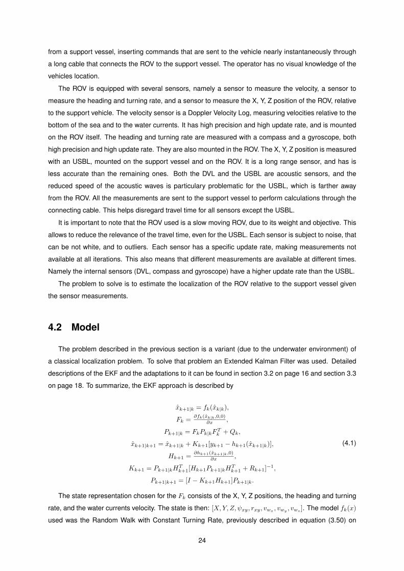
The problem described in the previous section is a variant (due to the underwater environment) of

a classical localization problem. To solve that problem an Extended Kalman Filter was used. Detailed

descriptions of the EKF and the adaptations to it can be found in section 3.2 on page 16 and section 3.3

on page 18. To summarize, the EKF approach is described by

xk+1|k = fk(xk|k),

Fk =∂fk(xk|k,0,0)

∂x ,

Pk+1|k = FkPk|kFTk +Qk,

xk+1|k+1 = xk+1|k +Kk+1[yk+1 − hk+1(xk+1|k)],

Hk+1 =∂hk+1(xk+1|k,0)

∂x ,

Kk+1 = Pk+1|kHTk+1[Hk+1Pk+1|kH

Tk+1 +Rk+1]−1,

Pk+1|k+1 = [I −Kk+1Hk+1]Pk+1|k.

(4.1)

The state representation chosen for the Fk consists of the X, Y, Z positions, the heading and turning

rate, and the water currents velocity. The state is then: [X,Y, Z, ψxy, rxy, vwx, vwy

, vwz]. The model fk(x)

used was the Random Walk with Constant Turning Rate, previously described in equation (3.50) on

24

and equation (3.52) on page 22. This model was chosen because the typical applications the

ROV is used include mostly navigation in the XY plane. The Z plane movement is used to emerge and

dives. The velocity inputs for the model uk, are the DVL measurements. They do not enter in the internal

state of the model.

To deal with outliers, the measurements are subjected to a threshold before being used in the filter.

This threshold is computed as described in equation (3.48). Delay of measurements is disregarded as

non existant, and the assynchronous measurement problem has no specific adaptation. The update is

done when there are measurements available and can be done partialy, i.e., only some values of the

internal state are updated.

25

Chapter 5

Simulations

In this section the simulation results of the filter estimation in multiple scenarios will be presented, in

order to show some detail on the particulars of the algorithm used to solve the problem. On the last part

of the section a simulated run was performed. This is the closest simulation to the real case, with all the

details previously considered all included. The simulations were all done using Matlab.

5.1 Model

In the previous section several models for the dynamics of the vehicle have been presented. In this

sub section two models are compared, to show how they behave in small intervals of dead reckoning.

The models compared are the Random Walk with Constant Velocity (RWCV) model and the Random

Walk with Constant Turning Rate (RWCTR) model, with a linear behaviour on the z axis. The RWCV is

a simpler model, assuming that the vehicle will move along a straight line, and tries to learn the velocity

vector, assuming it is constant, or at least constant in significant intervals. The model for the RWCV

can be found in equation (3.49). The RWCTR expects a more complex behaviour from the vehicle. It

predicts movement with a constant turning rate, which also includes the straight line of the RWCV. It

learns the turning rate and maintains the curvature on a dead reckoning scenario. Its’ model can be

found equation (3.50), using the matrix from equation (3.52).

In figure 5.1a on the next page and figure 5.1b on the following page one can see the behaviour of

both models in intervals of observations without noise and intervals of dead reckoning in a linear and

curving trajectory, in the XY plane. In the images the actual path of the vehicle is marked as a blue line,

named true. The observations made are without any noise and are marked in black cross symbols. The

estimated position of the vehicle is marked as red circles.

The observations allow for the filters to learn the parameters needed to make preditions on the dead

reckoning phase. In the linear phase, there is no significant difference between the RWCV and the

RWCTR, as one would expect. If the turning rate is zero, the RWCTR becomes the RWCV, only allowing

straight movement. As such, in the first phase both filters are equivelent.

In a curving trajectory however, the RWCV fails to correctly predict the behaviour of the vehicle. It

27

(a) Random Walk with Constant Turning Rate Model (b) Random Walk with Constant Velocity Model

Figure 5.1: Model Behaviour with Missing Measurements.

instead continues to follow the same line, as if were the same linear movement. This behaviour can

be seen in figure 5.2a and figure 5.2b, which show the curving part of the trajectory with more detail.

The images follow the same color scheme and symbols representation as figure 5.1a and figure 5.1b.

The RWCTR, assuming it has enough measurements to learn the turning rate before hand, is capable

of following the curve correctly. It uses the constant turning rate and correctly predicts the pose of the

vehicle during the curve. However, if left unaided it would simply continue to estimate a curve motion of

the vehicle, endlessly.

(a) Random Walk with Constant Turning Rate Model (b) Random Walk with Constant Velocity Model

Figure 5.2: Model Behaviour with Missing Measurements (Zoomed).

As the images show, the choice of the model may influence the accuracy of the results of the filter,

especially in the areas were the observations are missing. However a more complex model has more

variables that introduce more error sources for the estimation. If uneeded, they may perform poorly than

their simpler equivalent models. In a straight line trajectory with a significant noise from the sensors,

the usage of more sensor measurements by the RWCTR model inputs more noise into the filter. An

example of such errors is shown in table 5.1 on the next page. In the Z axis the models are equivelent

and as such the error on that axis is very similar.

If the noise of the sensors used by the RWCTR which are discarded by the RWCV is very small this

difference may not be relevant.

28

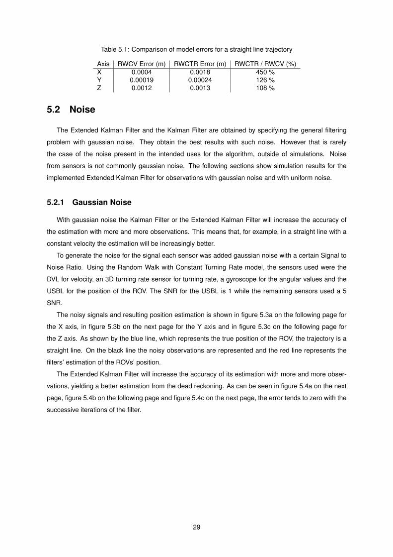
Table 5.1: Comparison of model errors for a straight line trajectory

Axis RWCV Error (m) RWCTR Error (m) RWCTR / RWCV (%)X 0.0004 0.0018 450 %Y 0.00019 0.00024 126 %Z 0.0012 0.0013 108 %

5.2 Noise

The Extended Kalman Filter and the Kalman Filter are obtained by specifying the general filtering

problem with gaussian noise. They obtain the best results with such noise. However that is rarely

the case of the noise present in the intended uses for the algorithm, outside of simulations. Noise

from sensors is not commonly gaussian noise. The following sections show simulation results for the

implemented Extended Kalman Filter for observations with gaussian noise and with uniform noise.

5.2.1 Gaussian Noise

With gaussian noise the Kalman Filter or the Extended Kalman Filter will increase the accuracy of

the estimation with more and more observations. This means that, for example, in a straight line with a

constant velocity the estimation will be increasingly better.

To generate the noise for the signal each sensor was added gaussian noise with a certain Signal to

Noise Ratio. Using the Random Walk with Constant Turning Rate model, the sensors used were the

DVL for velocity, an 3D turning rate sensor for turning rate, a gyroscope for the angular values and the

USBL for the position of the ROV. The SNR for the USBL is 1 while the remaining sensors used a 5

SNR.

The noisy signals and resulting position estimation is shown in figure 5.3a on the following page for

the X axis, in figure 5.3b on the next page for the Y axis and in figure 5.3c on the following page for

the Z axis. As shown by the blue line, which represents the true position of the ROV, the trajectory is a

straight line. On the black line the noisy observations are represented and the red line represents the

filters’ estimation of the ROVs’ position.

The Extended Kalman Filter will increase the accuracy of its estimation with more and more obser-

vations, yielding a better estimation from the dead reckoning. As can be seen in figure 5.4a on the next

page, figure 5.4b on the following page and figure 5.4c on the next page, the error tends to zero with the

successive iterations of the filter.

29

(a) Trajectory in X axis with Gaussian Noise (b) Trajectory in Y axis with Gaussian Noise

(c) Trajectory in Z axis with Gaussian Noise

Figure 5.3: Trajectory with Gaussian Noise

(a) Relative Error in X axis with Gaussian Noise (b) Relative Error in Y axis with Gaussian Noise

(c) Relative Error in Z axis with Gaussian Noise

Figure 5.4: Relative Error with Gaussian Noise

5.2.2 Uniform Noise

As most scenarios the noise from the sensors is not a gaussian noise, simulations were also per-

formed with uniform noise. The model used was still the Random Walk with Constant Turning Rate, on

a straight line trajectory. The USBL was generated with 0.5% noise and the DVL, the gyroscope and the

3D turning rate sensor signals were created with 0.1% noise. In equation (5.1) on the facing page more

30

detailed how the noises were generated is shown. The uniform function draws with equal probability a

real number between -1 and 1.

XUSBL = XUSBL + 0.005 ∗ uniform(−1, 1) ∗XUSBL (5.1)

The resulting noisy signals can be seen in figure 5.5a for the X axis, in figure 5.5b for the Y axis

and in figure 5.5c for the Z axis. While the uniform noisy signals start with less noise when comparing

with the gaussian noisy signals, over some iterations the noise becomes more influencial on the uniform

noisy signals. In the uniform case, it better mimics the increasing noise from the sensors with the greater

distance to the source of the sensor. If the sensor is not set at the (0, 0) point of the referential however,

the simulated observations will tend to be noisier than the actual sensor.

(a) Trajectory in X axis with Uniform Noise (b) Trajectory in Y axis with Uniform Noise

(c) Trajectory in Z axis with Uniform Noise

Figure 5.5: Trajectory with Uniform Noise

As seen in figure 5.6a on the following page, figure 5.6b on the next page and figure 5.6c on the

following page for the X, Y and Z axis, unlike the behaviour of the filter with gaussian noise sensors, with

uniform noise the accuracy of the estimation is not increasing with the successive iterations of the filter.

As discussed before, the Kalman filter behavious better in a gaussian environment. That remains true

for the Extended Kalman Filter, which can be seen as a generalization of the Kalman Filter.

31

(a) Relative Error in X axis with Uniform Noise (b) Relative Error in Y axis with Uniform Noise

(c) Relative Error in Z axis with Uniform Noise

Figure 5.6: Relative Error with Uniform Noise

5.3 Outliers

As discussed in section 3.3.3 on page 19, the sensor data has more error sources aside from noise.

Outliers can occur due to a varying of unpredictable situations, and can severily alter the estimation of

the filter, at least in a short time. This section presents the approach used to reject these outliers, by

using a covariance based dynamic threshold algorithm, already described in equation (3.48) on page 20.

For a specific percentage of outliers, the algorithm selects randomly that percentage of measure-

ments from the observational data. For each observation it is randomly selected a value from an uniform

probability function from 2 to 30. These values are multiplied by a uniform random variable that can

take the values 1 or −1. Finally they are multiplied by the actual value of the observation at that index

and added to the observation value.(noise has not been added at this point, but it will be added to the

outlier observation). In figure 5.7a on the next page (X axis), figure 5.7b on the facing page (Y axis) and

figure 5.7c on the next page (Z axis) we can see the resulting observations for 30% outliers, 0.1% noise

for the USBL and 0.01% noise for the remaining sensors. In figure 5.7d on the facing page we can see

the heading observations. In blue we can see the observations while in red there are the actual values

for the ROV.

32

(a) X axis (b) Y axis

(c) Z axis (d) Heading

Figure 5.7: Observations with 30% outliers and noise

In order to deal with the outliers, as mentioned before, a threshold is set based on the covariance

of the state estimation at that iteration. As more and more measurements are rejected, the threshold

increases allowing more noisy measurements to counter balance the extended period of dead reckoning

estimation. The outliers are rejected based on equation (3.47) on page 20, with the threshold being

computed based on equation (3.48) on page 20. As an example, figure 5.8a and figure 5.8b show how

the threshold evolves in the presence of noise but with no significant outliers, i.e., the outlier percentage

specified in the algorithm described before is zero. As expected, the threshold becomes centered on a

specific and low value, with its variations dependent on the noise in the measurements. For this case,

the threshold is stabilizing around the static minimum specified in equation (3.48) on page 20.

(a) Threshold for Outlier Rejection for Position (b) Threshold for Outlier Rejection for Heading

Figure 5.8: Threshold for Outlier Rejection with no Outliers

The tolerance threshold evolves dynamically with the algorithm, increasing as measurements are

rejected and decreasing as they are used to update the dead reckoning estimation. In figure 5.9a

on the following page and figure 5.9b on the next page we see the evolution of the threshold for the

observational data generated in figure 5.7a (X axis), figure 5.7b (Y axis) and figure 5.7c (Z axis). It starts

33

at an initial high value, to allow the filter to receive the first measurements independent of their noise, as

best seen in figure 5.8a on the previous page and figure 5.9a. It starts to decrease as more and more

measurements are accepted by the filter. The peaks seen in the figures correspond to observations

that were rejected, thus resulting in high covariance and higher threshold. The peaks reach higher and

higher values when the rejection happens for more iterations in a short span of time. The speed of

the threshold response to changes in the covariance can be tuned, by adjusting the parameter σ in

equation (3.48) on page 20. In the case of figure 5.9b the parameter is set to 0.5 and there is no mean

as n = 1, which results in a rapid response threshold with high and thin peaks as can be seen. In

figure 5.9a the σ is set to 1 but the n is equal to 3, making the scaling to 1/3 of the sum of the covariance

of the position measurements. This results in a slower response filter, with smaller but thicker peaks.

(a) Threshold for Outlier Rejection for Position (b) Threshold for Outlier Rejection for Heading

Figure 5.9: Threshold for Outlier Rejection

For five runs with these values the mean number of rejected outliers was 122, out of 500 measure-

ments. This means that around 24% outliers were rejected, with 30% of the observations being outliers.

5.4 Sensors Update Rate

The different sensors hava a different update rate, with the DVL and IMU sensors, which are placed in

the ROV, having a faster rate than the USBL, which is on the support vehicle. In the simulations this time

lapse between the sensors is done by removing observations between a certain number of iterations,

corresponding to the time between sensor measurements. Since the time between each iteration of the

filter is considered to be 0.1 seconds, for a update rate of 5 seconds for the USBL, there will be only

one USBL measurement for every 50 iterations. This means that only 2% of the iterations will have an

update measurement from the USBL. Naturally, for a slow update rate there will be a significant amount

of dead reckoning, especially regarding the position (USBL).

In figure 5.10a, figure 5.10b and figure 5.10c we have the example of the observations that reach

the filter, for a USBL with a 5 second update rate. This test run was made for 5000 iterations, with 100

USBL measurements. For the IMU sensors, in figure 5.10d on the facing page, we have an update rate

of 1 second (10% of the number of iterations), i.e., 500 measurements.

34



Figure 5.10: Noisy observations with a 5 second update rate for the USBL and 1 second update rate forthe remaining sensors.

The iterations with no observations will force the filter to estimate the results solely on dead reack-

oning, increasing the covariance of the estimation. This will impact the estimation negatively, with the

update rate of the measurements having a direct effect on the accuracy of the results. In figure 5.11a,

figure 5.11b, figure 5.11c and figure 5.11d, the covariance of the estimation for the conditions described

before.

(a) XX (b) YY

(c) ZZ (d) Heading

Figure 5.11: Covariance changes in estimated state.

35

For a more realistic scenario and a comparison to the conditions already presented, the next obser-

vations are generated with an USBL with a 2 second update rate. The remaining sensors have the same

update rate. As can be seen, although the pattern of covariance is similar, the amplitude of the covari-

ance is smaller, around half of the previous example. For the heading there is no significant difference,

as the sensor had the same update rate.

(a) XX (b) YY

(c) ZZ (d) Heading

Figure 5.12: Covariance changes in estimated state for a 2 second update rate USBL.

5.5 Noise Configuration Parameters

As previously introduced in section 3.1 on page 9, the noise that is input into the model affects the

weight given to observations or filter estimations when comparing the two in the update step. This can

be perceived as the filter designer trusting more on one or the other, resulting from the knowledge one

has over the system. In this section an example will be shown as how that change in noise parameters

affects the end result of the filter. The observational data will be generated with no outliers and there will

be observations in all iterations. Two sets of observations will be generated: one with high sensor noise

and one with low sensor noise but a significantly deviated initial position.

For the first example low noise sensors were used. A inaccurate starting position was used to show

the difference between high and low confidence in sensors. First, a filter with less confidence in sensors

was used. This means that the filter parameters have a high sensor noise to model noise ratio. It also

results in a less flexible filter, taking more time to adapt to changes in the observations. In this particular

case the observations were generated with 0.1 USBL noise and 0.01 DVL and IMU sensor noise.

The noise parameters introduced in the model are detailed on table 5.2 on the facing page for the

model parameters and table 5.3 on the next page for the observations used in the update step.

36

Table 5.2: Model Noise Parameters

Axis Noise ValueX 0.1 (m)Y 0.1 (m)Z 0.1 (m)

Heading 0.5 (o)Angular Rate 0.05 (o/s)

Water Current X 0.001 (m/s)Water Current Y 0.001 (m/s)Water Current Z 0.001 (m/s)

Table 5.3: Observational Noise Parameters

Axis Noise ValueX 500 (m)Y 500 (m)Z 500 (m)

Heading 50 (o)

The resulting estimation of the state and observational data are shown in figure 5.13a on the following

page, figure 5.13b on the next page, figure 5.13c on the following page and figure 5.13d on the next

page. In red is the estimated state, with the observational data represented as black crosses. Due to

the erroneous starting position the filter estimation runs alongside the true data. Due to the straight line

trajectory the dead reckoning has a better change of predicting the state than in more complex scenarios.

In table 5.4 the mean errors for the simulation are detailed. The number of rejected observations is 5000,

which means all observations were rejected, making this simulation a full dead reckoning case.

Table 5.4: Mean Errors for a Low Sensor Noise with Low Sensor Confidence

Axis Mean ErrorX 10.0082 (m)Y 25.0131 (m)Z 5.0138 (m)

Heading 0.0039 (o)

37

(a) X Axis (b) Y Axis

(c) Z Axis (d) Heading

Figure 5.13: Low sensor noise and high confidence in dead reckoning.

In the next scenario the filter has more confidence in sensors. The generated observations used

the same parameters as before. The filter parameters used are described in table 5.5 and table 5.6.

With the lower sensor noise the filter will respond more rapidly to changes in trajectory, by giving higher

weight to the sensors, in the states estimation.







Heading 0.5 (o)

The results of the simulation are depicted in figure 5.14a on the next page, figure 5.14b on the facing

page, figure 5.14c on the next page and figure 5.14d on the facing page. In table 5.7 on the next page the

mean errors are represented. The number of outliers rejected were 1490, mainly due to the erroneous

starting position.

38



Figure 5.14: Low sensor noise and high confidence in sensor measurements.

Table 5.7: Mean Errors for Low Sensor Noise with High Sensor Confidence


Heading 0.0039 (o)

In this scenario, due to the erroneous starting position and low sensor noise, the higher weight of

the observations allow the filter to quickly restore the accuracy of the estimation. High accuracy sensors

benefit a flexible filter, which can deal with rapid changes in trajectory correctly.

In the next case there will be higher noise. Compared to the previous scenario this will result in a

lower difference between low and high confidence in dead reckoning, as the SNR remains the primary

source of errors in the model. The noise observations where generated with a nosie of 1 for USBL and

0.1 for the remaining sensors. Note that, compared with the previous scenario, this is 10 times the noise

for the sensors.

For the first case there will be a high confidence in dead reckoning, with a approximately correct

starting position. The noise parameters introduced in the model are shown in table 5.8 on the following

page and in table 5.9 on the next page. In figure 5.15a on the following page and so on, we see the

resulting estimation compared with the noisy observations and the real data.

The number of rejected measurements was 4401, which is approximately 88%.

39







Heading 2.5 (o)



Figure 5.15: High sensor noise and high confidence in dead reckoning.

Table 5.10: Mean Errors


Heading 0.0384 (o)

The next case there is be a high confidence in the sensors, with an erroenous starting position. The

noise parameters introduced in the model are shown in table 5.11 on the next page and in table 5.12 on

the facing page. In figure 5.16a on the next page and so on, we see the resulting estimation compared

with the noisy observations and the real data.

40

The number of rejected measurements was 4379, which is also approximately 88%.







Heading 0.5 (o)



Figure 5.16: High sensor noise and high confidence in sensor measurements.

Table 5.13: Mean Errors


Heading 0.0385 (o)

As expected, the difference is much less perceptible than when in a low sensor noise scenario.

41

However such adjustments of the noise parameters can be used to fine tune the algorithm to the sensors

and model used.

5.6 Simulated Run

In this section a simulated test with all the specifics considered before was done. As before, a trajec-

tory was done from which observations were sampled to introduce in the filter. The discrete trajectory

had 5000 samples. From these samples the actual sensor data was less, since some were discarded to

simulated the sampling rate of the sensors. Noise was added, as detailed in the previous sections, and

outliers were introduced. The unsampled trajectory can be seen in figure 5.17. The trajectory is divided

into 2 parts. In the first section, until around the 2500th sample, it is a straight line with no accelera-

tion. In the next section, the trajectory corresponds to an ascending spiral, having a circular motion with

constant turning rate. This trajectory is a bottom-lock trajectory, i.e., the DVL is measuring the velocity

relative to the bottom of the water body, and the water velocity is always zero. The velocities of each

section are small, to match the actual ROVs sluggish motion. From this trajectory the USBL observa-

tional data was taken with a 3 second (30 measurements) sampling rate and the maximum noise was

10%. For the remaining sensors, the sampling rate was 1 second (10 measurements) and the noise

was 1%. The outliers introduced total in 10% of the measurements.

Figure 5.17: Trajectory (Unsampled).

The initialization of the filter was done with a high confidence in the model approach. The noise

parameters for the the observational data of the USBL was 25, and 2.5 for the heading. With the model

noise parameters, 0.1 was used for the X, Y, and Z axis. For the heading, the parameter was 0.5, and

0.05 for the turning rate. For the water velocity, since the trajectory was a bottom trajectory, the filter sets

the value of the corresponding parameters of the internal state to zero.

42

Figure 5.18: Simulated XY Plane

Figure 5.19: Simulated XY Plane [Zoomed In]

The outliers generated in the filter observations can be seen in figure 5.18, for the XY plane. To allow

for a more detailed understanding of the results of the simulation, figure 5.19 shows the same results

in a fixed frame. As seen in the figure, with a good initialization the filter can pinpoint the localization of

the ROV in the straight line trajectory without significant deviations. When the ROV as a more complex

trajectory, although still a trajectory predicted in the models description, the filter has more dificulties

following it. As one would expect, the estimation of the ROVs position by the filter in average has less

deviations from the actual position of the ROV than the sensors raw measurements. Even in the most

difficult parts of the trajectory, the estimation of the filter is still less error prone than the raw sensor

measurements.

Before analysing the actual numeric results of the simulation, it is important to have an overview of

43

the filter results for each axis. The Z axis, not shown in figure 5.19 on the previous page, has a linear

trajectory. This makes it easily followed by the filter, having the lowest deviation of the 3 axis. The full

result for the Z axis can be found in figure 5.20c, while a fixed frame version, not showing some of the

outliers, is found in figure 5.21c on the next page. For this simulation, the Z axis is being considered

relative to the bottom of the sea, unlike in the experimental run, when the measurements will be made

relatively to the supporting vessel.

The X axis, after the initial straight line trajectory, will begin a sinusoidal motion, characteristical of

the spiral trajectory. In figure 5.20a, the full results can be seen, while as before the more zoomed in

version is in figure 5.21a on the next page. As can be suspected by the XY plane results shown before,

the X axis estimation has more deviations from the true position of the ROV in the circular part of the

trajectory. The same can be said for the Y axis, found in figure 5.20b, and in more detail in figure 5.21b

on the next page.

For the heading, represented in figure 5.20d, there isn’t much relevance in viewing its detailed graph-

ical results, as it remains constant until the circular motion, where it is linear.



Figure 5.20: Simulation Results per Axis

44


(c) Z axis

Figure 5.21: Simulation Results per Axis [Zoomed In]

The average errors of the simulation can be found in table 5.14, in meters (for the X, Y and Z axis)

and in radians (for the heading). As one could expect from the graphical results shown before, the

heading as a very low error, as it is mostly constant and if not, linear. The second less error prone was

the Z axis, as it was always linear. Lastly, the X and Y axis have the largest errors. Considering that the

simulation has the highest X value as 30 meters, and around 50 for the Y axis, the average error can

be considered small. It must be noted, however, that the type of trajectory, starting at zero and growing

linearly in all 3 axis, is not irrelevant for that comparison.

Table 5.14: Simulaton Errors

Axis ErrorX 0.3138 (m)Y 0.5124 (m)Z 0.2991 (m)

Heading 0.0425 (o)

In order to further analyse the results, the outliers discarded, the evolution of the outliers threshold

and the innovation of the filter should be considered. As mentioned before, the number of outliers was

10 % of the 5000 measurements, 500. The number of measurements rejected was 765, a little over.

This may indicate, since there aren’t any significant deviations of the actual ROV trajectory, that all of the

outliers were rejected, as well as a few other measurements. Those measurements, while not generated

as an outlier, may have been measurements with higher noise, falling below the outlier threshold at that

particular time.

In figure 5.22a on the following page and in figure 5.22b on the next page it is shown the threshold

values during the simulation. Each threshold follows the pattern of being mostly constant, or linear vari-

ant, with peaks for areas where the filter was discarding several measurements. This results in a growing

45

threshold, mimicking the covariance of the estimation, to allow the filter to return to the approximate tra-

jectory when gone astray. Since the threshold is in absolute values, the peaks have higher amplitudes

to the latter part of the simulation, when the values for the axis are larger. Larger, higher and frequent

peaks would be a sign that the filters estimation was of high covariance. For this particular case, almost

all threshold values don’t go past the 5.3 meters mark, for the axis, which can be a indicator of a good

estimation, since the absolute values for the axis are around 30, 50 meters. It is important to remember

that the threshold having peaks is unavoidable, since the measurements are assynchronous and most

of the time there aren’t any sensor measurements.

(a) (X,Y,Z) axis (b) Heading

Figure 5.22: Evolution of Outliers Threshold

Innovation, as mentioned before, is another useful tool to understand if the dead reckoning estimation

was good, or if the sensor information is having a higher weight in the filters estimation. As can be seen

in figure 5.23a on the facing page, figure 5.23b on the next page and figure 5.23c on the facing page the

innovation for the pose is small, never exceeding one meter and being mostly below 0.2 meters. This

corroborates the previous indications that the estimation is accurate, and the sensor measurements is

not adding a high amount of information. For the heading innovation, in figure 5.23d on the next page,

there are higher peaks. They are not evenly spaced in the iteration axis, so one can infer that they

result from growing deviations on the heading estimate due to lack of measurements, or due to a small

threshold. These are few occurences however, as most of the iterations have a low innovation.

46



Figure 5.23: Evolution of Innovation

Although the results of the simulation can be considered satisfactory, it is important to note that they

were made for a trajectory that was predidect with the model. Although the noise and update rate of the

measurements was poorer than what can be achievied in some cases, the trajectory can have a bigger

weight and increase the difficulty of the filter to compute a good estimation. For ROVs, the modelling of

the trajectory is a problem which can be somewhat avoided, if the operator has a deep knowledge of the

model and avoids trajectories to distant from what was stipulated.

47

Chapter 6

Experimental Results

6.1 EMEPC

EMEPC is an acronym for Continental Platform Expansion Mission Estructure (Estrutura da Missao

de Espansao da Plataforma Continental). It is a portuguese project with the purpose of, as the name

implies, expanding the continental plataform through the use of technological innovation and research.

From its website: ”The EMEPC’s mission is to prepare and monitor the process of extending the con-

tinental shelf of Portugal. Given the nature of the work required to achieve this mission, the EMEPC

contributes to the enhancement of the technical and scientific skills required for deep sea operations,

projecting Portugal as a credible, internationally recognised partner.” [8].

The main goals of EMEPCs mission statement include (taken from [8]):

• To determine the geological and hydrographical features of the seabed off the coast of mainland

Portugal and the autonomous regions of the Azores and Madeira.

• To create a dictionary of oceanographic data and prepare the structure of a support database for

the Continental Shelf Extension Project (CSEP) so that, in the future, it may serve as a monitoring

and integrated ocean management system.

• To develop research and development projects oriented towards the exploitation of the information

and data obtained in the development of the CSEP.

• To engage the domestic scientific community through doctoral programmes related to the CSEP,

particularly in geology, geophysics and geographic information systems and public international

law.

• To promote the publication of an atlas of data and information relating to the CSEP.

• To encourage the participation of young students and researchers in the CSEP.

• To assist in the preparation of proposals for the extension of the continental shelf of States with

which the Portuguese Government may establish cooperation agreements in this area.

49

The EMEPCs project more relevant to this work in the investment in the ROV Luso, for up do 6000

meters deep sea exploration. During 2015, the EMEPC partnered with IST/ISR/LARSyS and CEiiA [8]

to perform exploration missions. The experimental data derived from those mission is used in this work.

These dives occured between the 25th of may and 3rd of june of 2015. More information about EMEPC

and its missions can be found in [8].

6.2 ROV Luso

The ROV Luso is a scientific Remotely Operated Vehicle that was adapted for collecting geological

and biological samples from the sea. The detailed technical specifications for the ROV Luso can be

found in [25].

Figure 6.1: ROV Luso. From http://www.emepc.pt/images/rov luso/ROV Equipamentos.jpg.

The most relevant sensors for this work present in the ROV Luso are:

• the Doppler Velocity Log (DVL), model WorkHorseNavigator 1200

• the Acoustic Positioning System (Ultra Short BaseLine), model TrackLink10000HA

• the Gyroscope, model KVHDSP3000

• the Compass, model KVHC100

• the Altimeter, model Kongsberg1007

50

• and the Depth Sensor, model SAIVDepthMeter

The remaining sensors can be found in [25]. Before continuing to the simulation and experimental

results, it is important to go into more detail on the workings of some of the sensors, and how each one

will provide the inputs for the model.

6.2.1 Ultra Short BaseLine

The ultra short baseline relies on a transceiver and computer in the supporting vessel that comu-

nicates with the module on the ROV in order to computed the X, Y, Z position of the ROV. The Track-

Link10000HA model, in particular, is described by its maker as a high accuracy, ultra long range USBL.

It has an accuracy of 0.25 degrees and can operate between 7.5 KHz up to 12.5 KHz. More detailed

information for the sensor can be found in [28].

The measurements obtained by this sensor are used as the X, Y and Z sensor readings.

6.2.2 Doppler Velocity Log

The Doppler Velocity Log is a sonar like sensor that uses four transducers to measure velocity relative

to a water body or to a fixed body. For the ROV Luso, this bottom mounted sensor measures velocity

relative to the bottom of the sea or relative to the water currents. The model used in the ROV Luso is

the Workhorse Navigator 1200. This sensor is very precise, with a long term precision of around 0.2%.

Specifications for this model can be found in [31].

The measurements of the DVL are used as inputs of the model, namely the velocity values. Unlike

other inputs, these are not used to update the internal state, since there isn’t any state representation for

the ROVs velocity. The high accuracy of this sensor is essential for this model to have sensible results.

6.2.3 Gyroscope and Compass

The gyroscope and compass are classical sensors, whose functionality is amply known. The DSP

3000 gyroscope model is a highly precise and high update rate sensor. Specifications for it can be found

in [7]. For the compass, the C100 model is a high accuracy sensor, with an error of around 0.5 degrees.

Specifications can be found in [5].

6.3 Experimental Results

In this sub section the results from a experimental run will be presented. Unlike the simulation, there

is no true data to rely on to determine the performance of the algorithm, so an analysis of the innovation

and the threshold will be used. In this case, the ROV does some exploration on a depth of around 300

meters and then emerges. The model and sensor noise parameters used are described in detail in

table 6.1 on the following page and in table 6.2 on the next page. The approach used was to consider

the both the model and observations at a similar relevance, giving no preferance to either. The water

51

current values are low, to try to mimic a small variance in them during the dive. This stems from the

idea that the water currents will not change significantly during a short period of time, and that there

aren’t many variations in the Z axis. Many and rapid variations in the Z axis could mean that the velocity

measurements are taken relatively to the water and the ground simultaneously during the experiment. It

is expected that this does not happen most of the time.



Heading 0.5 (o)





In figure 6.2 on the facing page the resulting XY Plane sensor measurements and estimated position

can be seen. Most of the iterations there is a similar result from the sensor measurements and the

estimated position. To better understand the results, in a global view, refer to table 6.3. In the table,

one can see that the mean innovation is very small, meaning that each sensor measurements adds little

information to the state. There are, however, large maximum jumps in the state, that can be a indicator

of the filter having a bad estimation in some iterations. It is important to note that, during the iterations,

only 8 measurements were rejected and not used to improve the state estimation.

Table 6.3: Innovation

Mean Median Max MinX (m) 0.0008245337 0 28.4922978425 -28.9512354263Y (m) -0.0026811340 0 23.8132059543 -22.6653105810Z (m) 0.0011582780 0 9.1854007155 -10.8842648895

Heading (o) 0.0088567783 0 418.4216264718 -390.2151369971Turning Rate (o/s) 0.0000070375 0 87.9691395753 -104.9881069366

Water Current (X) (m/s) -0.0000030799 0 0.1948231886 -0.1653758673Water Current (Y) (m/s) -0.0000036470 0 0.2763812590 -0.2317421161Water Current (Z) (m/s) 0.0000631134 0 0.6602620267 -0.8747413794

To better understand the quality of estimation in each of the position and heading parameters, the

detailed innovation and threshold evolutions are shown below.

52

Figure 6.2: XY Plane

To reiterate, the X axis follows a turning rate model, which straight and circular, with constant turning

rate, movements. In figure 6.3 on the following page the results of the estimations are shown. The black x

marks show all of the observations, including the rejected ones. The red line shows the filter estimation

for the X axis. Due to the order of the value of X, 10000, the scale can be deceiving when trying to

understand the sensor accuracy and the filters perfomance. Considering the number of measurements

rejected was 8, the filter closely follows the sensor observations.

In figure 6.4 on page 55, the innovation due to sensor information can be seen. There are spikes

which show times where the filter started to deviate from the sensors significantly. This behaviour is

expected however, as there are many iterations without measurements. As one could deduce from the

previous image, the innovation is mostly below 5 meters. The numerical results are detailed in table 6.4

on the following page, globally, and in table 6.5 on the next page in histogram form.

The maximum and minimum value of innovation are related with the peaks seen in figure 6.4 on

page 55. In the figure one can already have and idea of how often do these peaks occur. Altough the

mean may be affected by them, the histogram is a better alternative to understand the distribution of

innovation values. Looking at table 6.5 on the next page, the values of innovation higher than 10 or

lower than -10 are 6, which correspond to the 6 peaks in the figure.

The mean value of innovation is very small, which colaborates figure 6.3 on the following page, which

shows that the filter is always close to the sensor observations. The median value is not particulary

53

Figure 6.3: X Axis

relevant, and only shows that the filter equally over and underestimates the X axis.

Table 6.4: X Axis Innovation

Mean (m) Median (m) Max (m) Min (m)0.0008245337 0 28.4922978425 -28.9512354263

The histogram table 6.5 was generated without the zero values, considering only when there is

innovation. Looking closely at the histogram, one can see that around 91% of the innovations are

between -1 and 1 meters. 58% are between -0.1 and 0.1 meters. This suggest a good filter estimation

most of the time, considering that the scale of the X axis values are on the order of 10000.

Table 6.5: X Axis Innovation Histogram

Bins -10 -2 -1 -0.50 -0.10 -0.05 0 0.05 0.10 0.50 1 2 10Value 3 71 599 1268 1130 697 7216 804 1303 1282 613 90 3

54

Figure 6.4: X Axis Innovation

As was the case with the X axis, the Y axis also has a turning rate model, which straight and circular,

with constant turning rate, movements. In figure 6.5 on the following page we can see, similarly as the X

axis, that the filter is closely following the sensor measurements. Apart from a few spaced cases, there

does not seem to be a big innovation.

When looking at the innovation in figure 6.6 on page 57, most cases seem to fall below 2.5 meters.

The peaks are still present, as before, due to times where the filter was more significantly different from

the sensor observations.

Comparing the mean value for the innovation in the Y axis, it is around 50% higher than with the X

axis. This indicates that the Y axis has a poorer estimation, maybe due to a more complex and rapid

motion than the X axis, or to a more erratic sensor output. The maximum and minimum values are lower,

although don’t appear to be significantly so.

Table 6.6: Y Axis Innovation

Mean (m) Median (m) Max (m) Min (m)-0.0026811340 0 23.8132059543 -22.6653105810

Considering the histogram for the Y axis, one can see that 89% of innovations fall between -1 to

1 and that 57% are between -0.1 and 0.1. As with the X axis, this histogram is done ignoring the 0

values for innovation. These small values for most of the innovations indicate a stable and consistently

55

Figure 6.5: Y Axis

approximate estimation.

Table 6.7: Y Axis Innovation Histogram

Bins -10 -2 -1 -0.50 -0.10 -0.05 0 0.05 0.10 0.50 1 2 10Value 4 157 747 1229 1254 732 7057 800 1166 1164 655 110 4

Looking now again at the XY Plane, in figure 6.2 on page 53, one can say that the filter is successfully

estimating the position. Each sensor adds, on average, very little information, on the order of milimeters.

There are however, times when the filter starts diverging from the sensors, but never so much as to

required a significant number of iterations to return to a correct estimation.

56

Figure 6.6: Y Axis Innovation

For the Z axis, the motion is simpler. Assuming only dives and emerges, the Z axis motion predicted

by the model is linear. As seen in figure 6.7 on the next page this is only approximately true, as the

Z axis value is not constant during the deep sea exploration. Even though that is the case, the figure

seems to indicate that the filter is still able to estimate correctly the value for the Z axis.

When looking at the innovation, in figure 6.8 on page 59, the innovations appear to be smaller than

with the X and Y axis. Apart from the peaks, it is much smaller than 2.5, the value that the other 2 axis

seem be limited by.

The mean value of the innovations, seen in table 6.8, don’t seem to corroborate that though. It sits

between the Y axis and the X axis, although the minimum and maximum values are significantly lower.

Table 6.8: Z Axis Innovation

Mean (m) Median (m) Max (m) Min (m)0.0011582780 0 9.1854007155 -10.8842648895

Finally, looking at the histogram, the total number of non zero innovations were 5624. This falls far

below the 15079 of the previous two axis. 97% of the bins are situated below 1 and above -1, while only

15% are between -0.1 and 0.1. Comparing this with the previous axis, it shows that although the peaks

of innovation are smaller and there are less innovations, the innovations that exist are larger. The most

probable cause is the model predicting a linear behaviour on the Z axis, with is not the case.

57

Figure 6.7: Z Axis

Table 6.9: Z Axis Innovation Histogram

Bins -10 -2 -1 -0.50 -0.10 -0.05 0 0.05 0.10 0.50 1 2 10Value 1 4 123 1052 1283 236 333 252 1252 1069 119 15 8

The position estimate, made up by the three axis X,Y and Z, has a small innovation on average, on

the order of milimeters. The sensors are mostly not adding a lot of information. There is however one

sensor with a contribution not shown in the innovation. The DVL enters the filter in the predict stage,

having no internal state. It has naturally a big weight on the accuracy of the estimation, being one of the

sensors with the higher update rate. A small increase in the errors of the DVL could make a significant

difference on the results of the estimation.

58

Figure 6.8: Z Axis Innovation

The heading estimation, due to its nature, is prone to higher innovations around its limit value. The

filter does not take this into account, treating it like any other measurement. As such, the jumps in the

sensor from 360 degrees to 0 degrees will normally cause the filter to be erroneous during a number of

iterations. In figure 6.9 on the following page we can see that this happens a few times during the run.

The innovation, in figure 6.10 on page 61 has significant peaks because of this. Apart from those cases,

the filter seem to follow closely the sensor estimations.

In table 6.10, we can see that in average the innovation is still small, on the order of a millionth of a

degree. The maximum and minimum innovation is much higher than any other axis, due to these edge

cases.

Table 6.10: Heading Innovation

Mean (o) Median (o) Max (o) Min (o)0.0088567783 0 418.4216264718 -390.2151369971

For the histogram, a signficant portion of the innovations are still between the -1 and 1 values,

specifically 78%. It is smaller than the other axis, altough most of the innovations are below -0.1 and 0.1

(54%). These edge cases are few and far between, but if they were more proeminent the filter estimation

of the heading could suffer greatly.

59

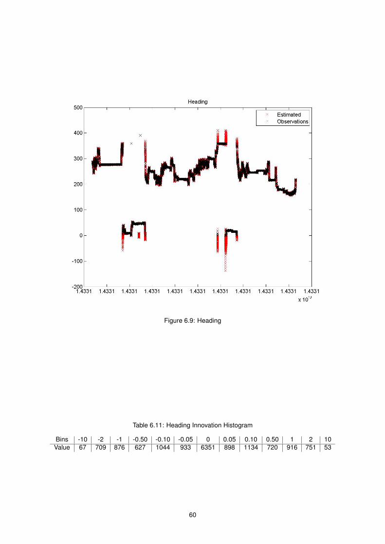
Figure 6.9: Heading

Table 6.11: Heading Innovation Histogram

Bins -10 -2 -1 -0.50 -0.10 -0.05 0 0.05 0.10 0.50 1 2 10Value 67 709 876 627 1044 933 6351 898 1134 720 916 751 53

60

Figure 6.10: Heading Innovation

61

Another factor to consider when analysing the performance of the filter is the threshold. The threshold

is dependent on the covariance of the estimation, growing in extended periods of dead reckoning. Since

the threshold is used to determine if a sensor measurement is an outlier, and reject it, its peaks also

indicate where there may have been measurements being rejected. The threshold used was divided

into a threshold for the position and a threshold for the heading.

In figure 6.11 on the next page the threshold evolution for the position, axis X, Y and Z, is represented.

The more problematic areas seem to be in the first part of the iterations, where there is an higher

covariance of the estimations. Due to the sheer number of interations, it is hard to understand completely

the details of the evolution of the threshold, and more general observations must be made. In table 6.12

the mean, median and limit values are shown. The threshold is capped between 5 and 55, but since the

covariance is never 0, as the estimation is never certain, the minimum value is a little higher than that. In

the figure we can see that the maximum value is only attained in the last iterations. Recalling figure 6.2

on page 53, and each individual axis figure shown before, these last iterations correspond to an area

where there are no sensor measurements. This means that the covariance simply increases with each

iteration, never diminishing.

From figure 6.11 on the facing page, the threshold values appear to be mainly a few specific values

distributed between the minimum and around 20. This seems to be due to the update rate of the

sensors. Each iteration the threshold increases to the next level and around 20 the next measurement

of the sensor is used, reverting the threshold back to a minimum value, by lowering the covariance. The

peaks correspond then to times where that measurement was discarded due to the innovation being

larger than the threshold.

Table 6.12: Position Threshold

Mean (m) Median (m) Max (m) Min (m)14.6682801442 13.1646615721 55.0000000000 5.9373129082

Taking a closer look at the histogram of the threshold, we can confirm what is seen in figure 6.11

on the next page. From the 89291 values, 95% of the threshold limits sit between the minimum value

and 20. The remaining 5% are then the areas where the filter was more divergente from the sensor

measurements.

Table 6.13: Position Threshold Histogram

Bins 6 7 9 13 16 20 25 30 50 100Value 5747 10505 16652 17429 20563 13896 1225 288 2986 0

This behaviour of the evolution of the threshold is, as was stated before, due to the update-rate nature

of the sensor measurements. It closely follows the covariance of the estimation, imposing a maximum

and minimum value.

62

Figure 6.11: Position Threshold

The heading threshold is severely affected by the edge cases seen before. From figure 6.12 on the

following page one can see that it has very high peaks. In table 6.14, the mean is very high. While the

minimum value is small, it seems that the threshold is systematically high. This means that, although

the innovations of each sensor were on average small, refering back to table 6.10 on page 59, the

covariance of the heading estimation is very high. It seems to be a weak point of the filter.

Table 6.14: Heading Threshold

Mean (o) Median (o) Max (o) Min (o)381.4702864541 350.0751030035 1471.2055903613 5.0397567123

Looking at the histogram, in table 6.15 on page 65, we can see that the values are much higher than

the previous measurements.

This indicates that although the innovations are small, the filter has little confidence on its estimation

of the heading value.

Refering back to table 6.3 on page 52, the filter has small innovation in each variable of the state. It

closely follows the sensors and, apart from special cases on the heading estimation, does not deviate

significantly during a significant number of iterations from the trajectory. This analysis is itself an indicator

only, as the actual values of each axis are not known, and the errors introduced by the sensors are

difficult to understand.

63

Figure 6.12: Heading Threshold

64

Table 6.15: Heading Threshold Histogram

Bins Value0 3553

45 736790 5380135 7081180 6728225 3855270 6156315 3776360 2347360 2757405 3573450 4962495 4082540 3765585 4168630 3067675 3509720 1394720 1025765 3183810 1845855 2280900 912945 726990 848

1035 2401080 712

65

Chapter 7

Conclusions

The localization and navigation problem in underwater environments is still an open problem, with

some classical approaches, such as the one presented in this work, and new algorithms inspired by

the successes of land robots. The restrictions of the underwater environment make this problem more

complex, due to the number of sensors that can be used and their cost. That being said, the underwater

navigation problem can be separated in three scenarios: surface, bottom and middle sea. The surface

scenario is the easiest of the three, having access to all technologies, namely GPS, for a precise lo-

calization of the Remotely Operated Vehicle (ROV). The bottom sea cames second in difficulty, as the

DVL can very accurately measure the velocity relatively to a fixed point (bottom of the sea). Although

the position is less accurate, having lost access to a GPS, the USBL can provide estimates. The mid-

dle depth scenario is the most problematic of the three. The precision of the USBL does not increase

signficantly, depending on the depth, and the DVL now measures the velocity relative to the water fluid.

This increases the amount of variables to determine, making the estimations more difficult to obtain.

The costs associated with the underwater problem are also higher than the ones associated with land

robots, either indoor or outdoor. Apart from the costs of the robot itself, there is always the necessity of

a supporting vessel, where the remainder of the sensors lie and normally where the computations are

made. Some sensor arrangements, such as a Long BaseLine, may require installations on the bottom

of the sea. These are of course expensive operations that reduce the number of configurations one can

use and try to develop an effective algorithm.

Apart from the limitation in terms of the number of sensors available and the costs of the sensors or

of their installation, the GPS signals poor penetration capacity in the aquatic medium also cause other

obstacles. The sensors used, namely the USBL, rely on acoustic waves. These travel at a signficant

lower velocity than electromagnetic waves and that time may not be negligible. This means that at a

certain iteration the measurements available may correspond to previous iterations only. For the specific

problem addresses this is not problematic, as the nature of the ROV implies that it moves slowly. This

means that one can safely discard the travel time of the acoustic waves.

The sensors used are also not equivalent in terms of update rate. This means that the ROV has

some measurements available at more iterations than others, and there are several iterations where

67

no measurement is available. This implies a significant portion of the estimation to be done in dead

reckoning. As with the travel time, the slow velocity of the specific ROV used mitigates this particular

problem.

This problem can be formulated as a localization problem. On a gaussian scenario, this problem

would be classically solved with a Kalman Filter, which gives the optimal solution for said problem.

Since the gaussian condition rarely holds in real world scenarios, the solution implemented was an

Extended Kalman Filter. To deal with the particulars described above, the EKF was adapted to perform

dead reckoning when no measurements were available, and to use measurements independently of one

another. To deal with outliers a threshold based on the covariance of the estimation was implemented,

rejecting severly deviated observations.

The model used to describe the trajectory of the ROV was a model that considered a trajectory

with constant turning rate in the XY plane, linear motion in the Z plane and in the heading axis. The

noise parameters of the model allowed for deviations of this model, and served as a factor between the

importance of the dead reckoning model and the observations in the filter estimation.

In the simulations chapter, the impact of each adaptation to the classical filter was discussed. The

controlled environment of a simulation allowed to analyse the specific modifications incrementally, with-

out having to view the final filter response only. The access to the actual position data also allowed

to have a better performance indicator of the filter. In the final section of the simulations chapter, a

simulation with the full filter was done. The filter could successfully follow the true positon, having a

better estimation of the position that the sensors measurements. The average errors were smaller than

1 meter on a trajectory that grows from the origin of the axis to a maximum of 30 in the X axis and 50 in

the Z and Y axis. The innovations and threshold were small, and the number of rejected measurements

was close to the number of outliers introduced in the measurements. The trajectory used was not highly

complex, and the limitations of the linearization of the model, tipical of the EKF, were not tested against

a filter without linearization, e.g., a Particle Filter.

In the experimental run, the filter could mostly follow the sensor measurements, with small average

values of innovation for each component. The water current was approximately zero, with the DVL

giving most measurements of velocity considering the bottom of the sea. There are a few peaks where

the filter was deviating significantly from the sensor values, but the increasing threshold due to the large

covariance allowed the filter to regain its course. The most problematic estimation was the heading,

which had large innovation values near the limits of the circle. If this where to be a more consistent

case, the filter should be adapted to deal with this situation, maybe through a transformation of the

sensor values to a more controlled degree interval.

The internal filter state not considering the DVL sensor values was not particulary damaging due to

the low noise of the sensor and its high update rate. When DVL measurements were not available, the

filter used the last available measurement, disregarding other sensor information. If the DVL had a lower

update rate, or if the sensor had higher noise, this could severely damage the estimation. Again, this

was not the case as the DVL is one of the most accurate sensors of the ROV and, being situated on the

ROV itself, has a high update rate of around 1 measurement per second.

68

Bibliography

[1] Anderson, Brian D.O., Moore, John B., in Optimal Filtering, 1st ed., New York, Doover Pub., 2005.

[2] Barkby, S., Williams, S., Pizarro, O., Jakuba, M., ”Bathymetric particle filter SLAM using trajectory

maps.”, J. Robot Res., vol 31, no 12, pp. 1409-1430, 2012.

[3] Bellingham, J., Vaganay, J., Leonard, J., ”Outlier rejection for autonomous acoustic navigation”,

Woods Hole Oceanographic Institution, Cambridge, MA, May, 1996.

[4] Brown, R., ”Integrated Navigation systems and Kalman fitlering: A perspective.”, Journal of the Insti-

tute of Navigation, vol. 19, 4, pp. 355-362, Winter 1972-1973.

[5] C100 Compass. Specifications at: http://www.emepc.pt/images/pdf/KVHC100.pdf

[6] Donovan, G., ”Position error correction for an autonomous underwater vehicle inertial navigation

system (INS) using a particle filter”, IEEE J. OCEAN, vol. 37, no. 3, pp. 431-445 , Jul. 2012.

[7] DSP 3000 Gyroscope. Specifications available at: http://www.emepc.pt/images/pdf/KVHDSP3000.pdf

[8] Estrutura da Missao de Expansao da Plataforma Continental (2015). Available at:

http://www.emepc.pt/

[9] Eustice, R., Whitcomb, L., Singh, H., & Grund, M., ”Recent advances in synchronous-clock one-way-

travel-time acoustic navigation”, IEEE OCEANS, pp. 1-6, Sep. 2006.

[10] Eustice, R., Singh, H., Leonard, J., & Walter, M., ”Visually mapping the RMS Titanic: Conservative

covariance estimates for SLAM information filters”, J. Robot Res, vol 25, no 12, pp. 1223-1242, Sep.

2006.

[11] Eustice, R., ”Large-area visually augmented navigation for autonomous underwater vehicles”, M.S.

thesis, Dept. Mec. Eng., Michigan State Univ., East Lansing, MI, 2005

[12] Henriksen, R., ”The truncated second-order nonlinear filter revisited”, IEEE Transactions on Auto-

matic Control, vol.27, pp. 247-251, 1982.

[13] Howell, B., Wood, S., ”Passive sonar recognition and analysis using hybrid neural networks”, Prov

OCEANS Conf., vol 4, pp. 1917-1924, 2003.

[14] Jalving, B., Gade, K., Hagen, O. K., & Vestgard, K., ”A toolbox of aiding techniques for the HUGIN

AUV integrated inertial navigation system”, IEEE MTS OCEANS, vol. 2, pp. 1146-1153, Sep. 2003.

69

[15] Kinsey, James C., Eustice, Ryan M., Whitcomb, Louis L., ”A Survey of Underwater Vehicle Naviga-

tion: Recent Advances and New Challenges”, 2006.

[16] Kinsey, J. C., ”Advances in Precision Navigation of Oceanographic Submersibles”, Ph.D. disserta-

tion, Dept. Mec. Eng., Johns Hopkins Univ., Baltimore, MD, 2006.

[17] Larsen, M., ”Syntethic long baseline navigation of underwater vehicles”, IEEE MTS OCEANS, vol.

3, pp. 2043-2050, Sep., 2000.

[18] Newman, P., Leonard, J., ”Pure range-only sub-sea SLAM”, Proc. IEEE Int. Conf. Robot Autom.,

vol 2, pp.1921-1926, Sep. 2003.

[19] Pascoal, A., Kaminer, L., Oliveira, P., ”Navigation System Design Using Time-Varying Complemen-

tary Filters”, IEEE TRANSACTIONS ON AEROSPACE AND ELECTRONIC SYSTEMS, vol. 36, 4,

pp. 1099-1114, Oct., 2000.

[20] Paull, L., Sacedi, S., Seto, M., & Li, H., ”AUV Navigation and Localization: A Review”, IEEE Journal

of Oceanic Engineering, vol. 39, pp. 131-149, Dec. 2013.

[21] Penas, A., ”Positioning and Navigation Systems for Robotic Underwater Vehicles”, Ph.D. disserta-

tion, DEEC, Instituto Superior Tecnico, Lisboa, Portugal, 2009.

[22] Ribas, D., Ridao, P., Tardos, J. D., Neira, J., ”Underwater SLAM in man-made structured environ-

ments”, J. Field Robot, vol. 25, no 11-12, pp 898-921, 2008.

[23] Ribas, D., Ridao, P., Mallios, A., Palomeras, N., ”Delayed State Information Filter for USBL-Aided

AUV Navigation”, IEEE International Conference on Robotics and Automation, Minnesota, USA,

May, 2012.

[24] Ribeiro, Maria Isabel, ”Kalman and Extended Kalman Filters: Concept, Derivation and Properties”,

IST, Lisboa, 2004.

[25] ROV Luso technical specifications.

Available at: http://www.emepc.pt/images/pdf/O ROV LUSO Descricao.pdf

[26] Simon, Dan., in Optimal State Estimation, 1st ed., Hoboken, New Jersey, USA/Canada, Wiley &

Sons, Inc., 2006.

[27] Space and Naval Warfare Command (2015).

Available at: http://www.public.navy.mil/spawar/Pacific/Robotics/Pages/CURV.aspx

[28] TrackLink 10000 USBL Sensor.

Specifications available at: http://www.emepc.pt/images/pdf/TrackLink10000.pdf

[29] Vaganay, J., Leonard, J., Bellingham, J., ”Outlier Rejection for Autonomous Acoustic Navigation”,

MIT, USA

70

[30] Walter, M., Eustice, R., Leonad, J., ”Exactly sparse extended information filters for feature-based

SLAM”, Int. J. Robot. Res., vol 26, no 4, pp.335-359, 2007.

[31] Workhorse DVL. Specifications available at: http://www.emepc.pt/images/pdf/workhorseNav.pdf

71

an advanced navigation system for remotely operated ... · sums up the study on classical problems...

Documents