an adaptive simulated annealing method for …
TRANSCRIPT
AN ADAPTIVE SIMULATED ANNEALING METHOD FOR ASSEMBLY
LINE BALANCING AND A CASE STUDY
A THESIS SUBMITTED TO
GRADUATE SCHOOL OF NATURAL AND APPLIED SCIENCES
OF
MIDDLE EAST TECHNICAL UNIVERSITY
BY
HÜSEYİN GÜDEN
IN PARTIAL FULFILLMENT OF THE REQUIREMENTS
FOR
THE DEGREE OF MASTER OF SCIENCE
IN
INDUSTRIAL ENGINEERING
AUGUST 2006
Approval of the Graduate School of Natural and Applied Sciences
Prof. Dr. Canan ÖZGEN Director
I certify that this thesis satisfies all the requirements as a thesis for the degree of Master of Science. Prof. Dr. Çağlar GÜVEN Head of the Department This is to certify that we have read this thesis and that in our opinion it is fully adequate, in scope and quality, as a thesis for degree of Master of Science. Asst. Prof. Dr. Sedef MERAL Supervisor
Examining Committee Members: Assoc. Prof. Dr. Levent KANDİLLER (METU, IE)
Asst. Prof. Dr. Sedef MERAL (METU, IE)
Prof. Dr. Hadi GÖKÇEN (Gazi U., IE)
Onur ÖZKÖK (Baskent U., IE)
Asst. Prof. Dr. Bayram Ali SU (Atılım U., IE)
iii
I hereby declare that all information in this document has been obtained
and presented in accordance with academic rules and ethical conduct. I
also declare that, as required by these rules and conduct, I have fully cited
and referenced all material and results that are not original to this work.
Name, Last name : Hüseyin, GÜDEN
Signature :

iv
ABSTRACT
AN ADAPTIVE SIMULATED ANNEALING METHOD FOR
ASSEMBLY LINE BALANCING AND A CASE STUDY
Güden, Hüseyin
M.Sc., Department of Industrial Engineering
Supervisor: Asst. Prof. Dr. Sedef Meral
August 2006, 195 pages
Assembly line balancing problem is one of the most studied NP-Hard
problems. NP-Hardness leads us to search for a good solution instead of the
optimal solution especially for the big-size problems. Meta-heuristic
algorithms are the search methods which are developed to find good solutions
to the big-size and combinatorial problems. In this study, it is aimed at solving
the multi-objective multi-model assembly line balancing problem of a
company. A meta-heuristic algorithm is developed to solve the deterministic
assembly line balancing problems. The algorithm developed is tested using the
test problems in the literature and the the real life problem of the company as
well. The results are analyzed and found to be promising and a solution is
proposed for the firm.
Keywords: Assembly Line Balancing, Multi-Model Line, Multi-
Objective, Meta-Heuristics, Adaptive Simulated Annealing
v
ÖZ
MONTAJ HATTI DENGELEMESİ İÇİN BİR UYARLANABİLİR
TAVLAMA BENZETİMİ YÖNTEMİ VE BİR ÖRNEK ÇALIŞMA
Güden, Hüseyin
Yüksek Lisans, Endüstri Mühendisliği Bölümü
Tez Yöneticisi: Y. Doç. Dr. Sedef Meral
Ağustos 2006, 195 sayfa
Montaj hattı dengeleme problemi en çok çalışılan NP-Zor
problemlerden biridir. NP-Zorluk, özellikle büyük boyutlu problemlerde, en iyi
çözüm yerine iyi bir çözümü araştırmamıza neden olur. Modern-sezgisel
algoritmalar büyük boyutlu ve kombinatoryal problemlere iyi çözümler bulmak
amacıyla geliştirilmiş yöntemlerdir. Bu çalışmada, bir şirketin çok-amaçlı çok-
modelli montaj hattı dengeleme problemini çözmek amaçlanmıştır. Bir
modern-sezgisel algoritma geliştirilmiş ve deterministik montaj hattı
dengeleme problemlerini çözmek üzere sunulmuştur. Geliştirilen algoritma
literatürdeki test problemleri ve şirketteki gerçek hayat problemi kullanılarak
test edilmiştir. Sonuçlar analiz edilmiş ve umut verici bulunmuşlardır ve firma
için bir çözüm önerilmiştir.
Anahtar Kelimeler: Montaj Hattı Dengeleme, Çok-Modelli Hat, Çok-
Amaç, Modern-Sezgiseller, Uyarlanabilir Tavlama Benzetimi

vi
To my family

vii
ACKNOWLEDGMENTS
I express my great gratitude to Asst. Prof. Dr. Sedef MERAL because
of her guidance and contributions throughout the study. I am indebted to İlker
İPEKÇİ, my friend, for his invaluable help. I also want to thank to Asst. Prof.
Dr. Haldun SÜRAL for his suggestions. Thanks to Yiğit Koray GENÇ, my
friend, for his contributions.

viii
TABLE OF CONTENTS
PLAGIARISM ................................................................................................ iii
ABSTRACT .....................................................................................................iv
ÖZ ..................................................................................................................... v
DEDICATION ................................................................................................ vi
ACKNOWLEDGMENTS .............................................................................vii
TABLE OF CONTENTS ..............................................................................viii
LIST OF TABLES ..........................................................................................xi
LIST OF FIGURES .......................................................................................xv
CHAPTER
1. INTRODUCTION ........................................................................................1
2. ASSEMBLY LINE BALANCING AND THE RELEVANT
LITERATURE ............................................................................................ 6
2.1 Assembly Lines ................................................................................... 6
2.2 Assembly Line Balancing Problem ................................................... 9
2.2.1 Single-Model Deterministic ALBP ...........................................10
2.2.1.1 Single-Model Deterministic Type-I ALBP .......................12
2.2.1.1.1 Optimal Seeking Methods .........................................12
2.2.1.1.2 Heuristic Solution Approaches .................................19
2.2.1.2 Single-Model Deterministic Type-II ALBP .....................20
2.2.2 Mixed-Model ALBP ..................................................................21
2.2.3 Multi-Model ALBP ....................................................................26
2.2.4 Meta-Heuristic Approaches ......................................................28
3. THE CASE STUDY ...................................................................................34
3.1 The Company in the Study .............................................................34
3.2 Current Balancing Method and Development of the Proposed
Method ............................................................................................34
3.3 Determining the Problem ................................................................37
ix
3.3.1 Tasks ...........................................................................................37
3.3.2 Task Times .................................................................................38
3.3.3 Precedence Relationships Diagram ..........................................39
3.3.4 Zoning Restrictions ....................................................................42
3.4 Integer Programming Studies ..........................................................45
4. THE PROPOSED APPROACH ...............................................................49
4.1 Simulated Annealing (SA) ................................................................49
4.2 Adaptive Simulated Annealing (ASA) .............................................51
4.3 Construction of the Solutions ...........................................................54
4.4 Representation of the Solutions ........................................................55
4.5 Types of Moves ..................................................................................56
4.6 Objectives of ALBP and Evaluation of Solutions ...........................57
4.6.1 Minimization of the Number of Stations .................................57
4.6.2 Minimization of Cycle Time .....................................................58
4.6.3 Maximization of Irregularity between Station Times ............59
4.6.4 Maximization of Smoothness between Station Times ............61
4.6.5 Maximization of Common Tasks that Assigned to the Same
Stations between Consecutive Models .....................................62
4.7 Sequencing Problem ..........................................................................63
4.8 The Proposed Methodology...............................................................63
4.8.1 Representation of the Solutions ................................................64
4.8.2 The Move Procedure .................................................................67
4.8.3 The Adaptive Cooling Schedule ...............................................68
4.8.4 Construction of the Initial Solution .........................................70
4.8.5 Evaluating the Solutions ...........................................................70
4.8.5.1 Evaluating the Line Balances ............................................70
4.8.5.2 Evaluating the Sequences ..................................................73
4.8.6 The Overall Methodology .........................................................74
5. EXPERIMENTAL ANALYSIS ............................................................... 77
5.1 Design of the Experiment ..................................................................77
5.2 Single and Mixed-Model Assembly Line Balancing Problems ….79
x
5.2.1 Test Problems .............................................................................79
5.2.1.1 The First ASA Part ............................................................79
5.2.1.2 The Second ASA Part ........................................................80
5.2.2 The Case Problem ......................................................................81
5.3 Multi-Model Assembly Line Balancing Problems ..........................85
5.4 Current Line Balance and Suggested Line Balances .....................88
5.5 Run Times of the Experiments .........................................................88
6. CONCLUSION AND FURTHER RESEARCH ISSUES .......................90
REFERENCES ...............................................................................................96
APPENDICES
A. SKETCH OF THE ASSEMBLY LINE OF THE FIRM .....................105
B. TASK LIST ..............................................................................................106
C. PRECEDENCE RELATIONSHIPS ......................................................116
D. PSEUDOCODE OF THE ALGORITHM .............................................128
E. RESULTS OF THE EXPERIMENTAL RUNS ...................................131
F. CURRENT AND SUGGESTED ASSIGNMENTS ..............................188
xi
LIST OF TABLES
TABLES
Table 4.1 Computations of station numbers and station times for the
example ................................................................................56
Table 4.2 Representations of the current and candidate solution in the
example with standard and order encoding ..........................65
Table 4.3 Differences between current and candidate solution of the
example according to standard and order encoding .............66
Table 5.1 Average values and Standard Deviation values of response
variables of 10 runs of SMALB and MiALB ......................82
Table 5.2 Average values of response variables of 10 runs for
MuALB ................................................................................87
Table B.1 Task List ..............................................................................106
Table C.1 List of immediate predecessor-successor relationships for
individual models ...............................................................116
Table E.1 Test problems and deviations of the found solutions from the
optimum solutions for SALBP-I. .......................................131
Table E.2 Descriptive statistics of deviations for SALBP-I ................137
Table E.3 Test problems and deviations of the found solutions from the
optimum solutions for SALBP-II. ......................................138
Table E.4 Descriptive statistics of deviations for SALBP-II ...............144
Table E.5 Sequences and number of common tasks between successive
models in a sequence. .........................................................145
Table E.6 Average values of common tasks that are assigned to the same
stations with low level of the weight of the third
objective .............................................................................146
xii
Table E.7 Average values of common tasks that are assigned to the same
stations with intermediate level of the weight of the third
objective .............................................................................147
Table E.8 Average values of common tasks that are assigned to the same
stations with high level of the weight of the third
objective .............................................................................148
Table E.9 Average values of TSTs at the beginning of the runs with low
level of the weight of the third objective ...........................149
Table E.10 Average values of TSTs at the end of the runs with low level
of the weight of the third objective ....................................150
Table E.11 Average values of numbers of stations at the beginning of the
runs with low level of the weight of the third objective ....151
Table E.12 Average values of numbers of stations at the end of the runs
with low level of the weight of the third objective ............152
Table E.13 Average values of the differences between the theoretical
minimum numbers of used stations and the numbers of used
stations found with the algorithm at the end of the runs with
low level of the weight of the third objective ....................153
Table E.14 Average values of cycle times at the beginning of the runs
with low level of the weight of the third objective ............154
Table E.15 Average values of cycle times at the end of the runs with low
level of the weight of the third objective ...........................155
Table E.16 Average values of the differences between the theoretical
minimum cycle times and the cycle times found with the
algorithm at the end of the runs with low level of the weight
of the third objective ..........................................................156
Table E.17 Average values of TSTs at the beginning of the runs with
intermediate level of the weight of the third objective ......157
Table E.18 Average values of TSTs at the end of the runs with
intermediate level of the weight of the third objective ......158
xiii
Table E.19 Average values of numbers of stations at the beginning of the
runs with intermediate level of the weight of the third
objective .............................................................................159
Table E.20 Average values of numbers of stations at the end of the runs
with intermediate level of the weight of the third
objective .............................................................................160
Table E.21 Average values of the differences between the theoretical
minimum numbers of used stations and the numbers of used
stations found with the algorithm at the end of the runs with
intermediate level of the weight of the third objective ......161
Table E.22 Average values of cycle times at the beginning of the runs
with intermediate level of the weight of the third
objective .............................................................................162
Table E.23 Average values of cycle times at the end of the runs with
intermediate level of the weight of the third objective ......163
Table E.24 Average values of the differences between the theoretical
minimum cycle times and the cycle times found with the
algorithm at the end of the runs with intermediate level of the
weight of the third objective ..............................................164
Table E.25 Average values of TSTs at the beginning of the runs with
high level of the weight of the third objective ...................165
Table E.26 Average values of TSTs at the end of the runs with high level
of the weight of the third objective ....................................166
Table E.27 Average values of numbers of stations at the beginning of the
runs with high level of the weight of the third objective ...167
Table E.28 Average values of numbers of stations at the end of the runs
with high level of the weight of the third objective ...........168
Table E.29 Average values of the differences between the theoretical
minimum numbers of used stations and the numbers of used
stations found with the algorithm at the end of the runs with
high level of the weight of the third objective ...................169
xiv
Table E.30 Average values of cycle times at the beginning of the runs
with high level of the weight of the third objective ...........170
Table E.31 Average values of cycle times at the end of the runs with
high level of the weight of the third objective ...................171
Table E.32 Average values of the differences between the theoretical
minimum cycle times and the cycle times found with the
algorithm at the end of the runs with high level of the weight
of the third objective ..........................................................172
Table F.1 Current and Suggested Assignments ...................................188

xv
LIST OF FIGURES
FIGURES
Figure 2.1 Types of Assembly Lines (Wild, 1972) .....….........................8
Figure 2.3 A combined precedence diagram constructed from two
models ..................................................................................23
Figure 4.1 An example of the convergence of a SA algorithm with very
small initial temperature .......................................................51
Figure 4.2 An example of the convergence of a SA algorithm with very
high initial temperature ........................................................51
Figure 4.3 An example of the convergence of an ASA .........................53
Figure 4.4 An example of the conventional cooling schedule of a SA
algorithm (Example 1) .........................................................53
Figure 4.5 An example of the conventional cooling schedule of a SA
algorithm (Example 2) .........................................................53
Figure 4.6 An example of the cooling schedule of an ASA algorithm ..54
Figure 4.7 Precedence Diagram of the Example ....................................56
Figure 4.8 Current and candidate solutions for the example .................60
Figure 4.9 Precedence Diagram of the Example ....................................65
Figure 4.10 An example of cooling schedule of the developed ASAs ..69
Figure 4.11 Flow chart of the methodology ...........................................76
Figure A.1 Sketch of the Assembly Line of the Firm ..........................105
Figure C.1 Combined precedence diagram ..........................................127
Figure E.1 Model1-number of used stations ........................................173
Figure E.2 Model1-cycle times ............................................................174
Figure E.3 Model1-total slack times ....................................................175
Figure E.4 Model2-number of used stations ........................................176
Figure E.5 Model2-cycle times ............................................................177
Figure E.6 Model2-total slack times ....................................................178
xvi
Figure E.7 Model3-number of used stations ........................................179
Figure E.8 Model3-cycle times ............................................................180
Figure E.9 Model3-total slack times ....................................................181
Figure E.10 Model4-number of used stations ......................................182
Figure E.11 Model4-cycle times ..........................................................183
Figure E.12 Model4-total slack times ..................................................184
Figure E.13 Combined-number of used stations .................................185
Figure E.14 Combined-cycle times .....................................................186
Figure E.15 Combined-total slack times .............................................187
1
CHAPTER 1
INTRODUCTION
Assembly line production is a production type, which is especially
suitable for mass production. The production system runs with a high
production rate and it is assumed that there is enough demand that can
consume this production.
Assembly line balancing offers many benefits such as increased
productivity, production of high amount of standardized items at low costs, less
work congestion, reduced material handling, etc.
In order to realize the production, there are some tasks that have to be
performed. Assembly lines are the production lines through which these tasks
are performed following the sequential stations. At the assembly lines,
production parts flow from a previous station to the next one. Because of this
fixed and directed flow, the tasks have to be assigned to the sequential stations
such that no part goes back to be reprocessed. The precedence relationships
between the tasks show the order of the tasks to be completed. Any task cannot
be performed before the tasks that are located in front of itself on the
precedence relationships diagram. The assembly line balancing is allocating the
tasks to the stations on the line such that all precedence relationships are
satisfied and the production is realized with the directed production flow.
Cycle time is the time between two parts’ passing from one station to
the next one. It can be assumed that each station has this time capacity which
cannot be exceeded.

2
Assembly lines can be classified into three groups, namely, single-
model lines which are dedicated to the production of a single product, multi-
model lines on which two or more similar models of products are produced
separately in batches and mixed-model lines on which two or more similar
models of a product are produced simultaneously on the line where the batch
sizes are very small or even one.
Real life problems are complex problems. When the problem includes
more than one and conflicting objectives, it gets harder to solve the problem.
Assembly line balancing problems, especially multi/mixed-model assembly
line balancing problems, are complex problems and generally consist of more
than one and conflicting objectives. Number of used stations, cycle time, idle
times, common tasks between models, setup cost for switching from
production of a model to another one’s, etc. are some of the components that
affect the solution of the assembly line balancing problems.
Especially for the multi-model assembly lines, the sequencing problem
arises as another problem besides the balancing problem. Because the common
tasks between the sequential models change with respect to the models, it
becomes important to determine the best sequence. If so, without balancing the
line for each model, determining the best sequence of the models arises as
another problem.
In today's industries and global market, due to the increasing
competitiveness, companies try to enhance production flexibility by reducing
their batch sizes and increasing product varieties. Because of this
competitiveness, single-model production is less common than multi/mixed
model production.
Although, based on our limited observations, multi/mixed-model
assembly lines are more preferred in real life, literature includes much more
3
studies on the single-model line. Therefore, the main motivation of our study
for working on multi/mixed-model assembly lines stems from these
observations. During our study on a real life multi-model assembly line
balancing problem, we have faced with many kinds of details, complexities and
very flexible structures on the line. In real life, assembly line balancing
problems proved to be much more difficult than in theory. We spent a lot of
time and effort to deal with these difficulties but it somehow motivated us.
The firm in the study produces consumer durables. It is one of the
companies that continue their production with different models. The firm
develops new models and produces different models in a continuous manner. It
also modifies its standard models according to customer specifications. But, the
ratio of these modifications is very small. Recently, the firm especially
produces four main models with high amounts.
There is no precedence relationships diagram in the firm. Assignments
are made manually by trial and error approach based on personal experiences.
Daily production is adjusted according to the production plans on some
monthly periods. Then, the line is balanced such that it satisfies this production
rate. Batch sizes of the different models are omitted. Similarities and common
tasks between models and consequently, sequence of the models are also
neglected.
Production seriously becomes inconsistent at the week that balancing is
made. This is an important disadvantage of the current balancing procedure.
Rarely, a few amount of products from a different model passes throughout the
line among other models. But, generally system works with large batch sizes
and as a multi-model assembly line. Balancing the multi-model assembly line
as if it is a mixed-model assembly line is another disadvantage of the current
procedure. Because of the lack of the objective functions goodness of the
obtained solution is not known. Furthermore, due to the lack of evaluating
4
functions and difficulty of the current method, better solutions may not be
searched. This is another disadvantage of the current procedure.
Meta-heuristic approaches are recently developed general search
strategies. When the problem sizes get larger, the computational times to solve
an NP-Hard problem increase non-polinomially. Especially solving the big-size
NP-Hard and combinatorial problems optimally becomes very hard, even
impossible.
This study proposes a new approach which is based on the Simulated
Annealing, one of the meta-heuristic approaches, to solve assembly line
balancing problems. The developed algorithm solves the multi-objective single,
mixed and multi-model assembly line balancing problems in a heuristic
manner. For illustrative purposes, the algorithm is used to solve the real life
multi-model assembly line balancing problem of the firm under consideration.
The proposed algorithm is tested on test problems from the literature
and on the case problem. For each type of assembly line balancing problems
the experimental results are analyzed separately and found to be promising.
With this study, it is achieved to find very good solutions even optimal
solutions, but it is not guaranteed, to complex assembly line balancing
problems in reasonable computational times. For the specific case of the firm
the method eradicated the disadvantages of the current method of the firm.
The thesis includes five chapters. The concepts related to Assembly
Line Balancing and the techniques used to solve Assembly Line Balancing
Problems are discussed in Chapter 2. The real life multi-model assembly line
balancing problem under consideration and its environment are defined in
Chapter 3. Besides, the difficulties related to the problem at hand and the
process of the development of the solution method proposed are discussed in
Chapter 3. In Chapter 4, the proposed solution method is explained. In

5
Chapter 5, the experimental results are analyzed and the study is concluded in
Chapter 6.

6
CHAPTER 2
ASSEMBLY LINE BALANCING AND THE RELEVANT
LITERATURE
2.1 Assembly Lines
When a product or a family of technologically similar products exhibits
high volume and stable demand over lengthy periods of time, it becomes
economical to design and layout a special facility dedicated exclusively to the
product or family of products under consideration. In order to cut down
work-in-process inventory and nonproductive times as loading, unloading and
transportation between successive operations, the workstations are physically
arranged in a contiguous sequence according to the technological ordering of
the manufacturing stages. The resulting facility is called an assembly line if the
production process is assembly or fabrication line if it is fabrication (Hax and
Candea, 1984).
Assembly is a production system and it is defined as the aggregation of
all necessary tasks in order to form a product.
Assembly is usually realized on assembly lines. Assembly line is a set of
workstations which are sequentially arranged and connected by means of a
transfer system.
Assembly lines can be classified with respect to the variety of models
assembled and the batch sizes of the models as:
7
• Single-model Assembly Line
• Multi-model Assembly Line
• Mixed-model Assembly Line
Single-model assembly line is the line on which only one model product
assembly is realized. The assembly line on which the batch production of more
than one similar model of products is realized is called multi-model assembly
line. Mixed-model assembly line is the line on which the simultaneous
production of more than one model of products takes place (Wild, 1972). (See
Figure 2.1).
Manufacturing a product on an assembly line requires partitioning the
total amount of work into a set of elementary operations named tasks (Scholl
and Becker, 2004). A task is the smallest indivisible work element that adds
value to the product. Performing a task requires certain equipment, machines
and/or skills of workers and takes some time called task time.
A workstation (or just station) is a location along the assembly line
where a subset of tasks is processed. To perform these set of tasks, a
workstation consists of human and/or robotic operators and equipment.
The sum of the task times of all tasks that are assigned to a workstation
(i) is called work content (WCi) of the workstation. A predetermined amount of
time allocated to each workstation to finish the tasks assigned to it is called the
cycle time (C). Cycle time is equal to the biggest work content and it
determines the time between two successive products passing from any fixed
point of the assembly line. In other words, cycle time is the time between two
successive products’ completions. Hence, the production rate of the assembly
line is 1/C. Slack time (or idle time) (STi) of a station (i) is the time difference
between cycle time and the work content of that station. The sum of the work
contents of all stations, or equivalently the sum of the task times of all tasks, is

8
called the total work content (TWC) and the sum of slack times of all stations
is called the total slack time (TST) or balance delay (BD). Assembly time (AT)
is the maximum time that the line may use to complete a product. Assembly
time is equal to multiplication of number of stations (m) and cycle time
(Baybars, 1986; Held, Karp and Sareshian, 1963; Klein, 1963; Kilbridge and
Wester, 1961; Kilbridge and Wester, 1962).
Figure 2.1 Types of Assembly Lines (Wild, 1972)
Stocks of parts to be assembled
a) Single-Model Assembly Line
Basic item fed
into the line
Assembly Line
b) Multi-Model Assembly Line
c) Mixed-Model Assembly Line
9
In order to realize the production, all tasks have to be performed. At the
assembly lines, products move from a previous station to the next station.
Because of this fixed and directed flow, the operations have to be assigned to
sequential stations such that no part goes back to be reprocessed. Some tasks
can not be performed until some other tasks are completed. These precedence
relations restrict the assignment of tasks to the workstations. A task can not be
assigned to the previous stations of the station that any previous task of that
task is assigned. The graph that shows precedence relations of tasks is called
precedence graph. It contains a node for each task, node weights for the task
times and arcs for the precedence constraints (Scholl and Becker, 2004).
Especially for the real life problems, zoning restrictions add further
complexities to the problem. Sometimes, there can be such situations that a set
of tasks has to be performed at the same station or different stations.
Occasionally, because of particular equipment, a task would be made at any
specific station or a task can not be performed at a particular station.
2.2 Assembly Line Balancing Problem
Assembly lines rely heavily on the Principle of Interchangeability and
the Division of Labor. Principle of interchangeability suggests that individual
components that make up a finished product should be interchangeable
between product units. Division of labor includes the concepts of work
simplification, standardization and specialization. These two concepts
facilitated mass production, allowed replacement parts to be used to lengthen a
product's useful life and made the development of assembly lines possible
(Askin and Standridge, 1993).
The first assembly line is credited to Henry Ford in 1915 after which it
has been widely used in various production systems (Erel, Sabuncuoğlu and
Aksu, 2001).

10
Assembly line balancing is allocating the tasks, which have to be
performed to manufacture the product, to workstations such that all precedence
relations and zoning restrictions are satisfied, taking into account cycle time
and/or number of workstations and task times. Assembly line balancing
problem (ALBP) is finding an allocation that optimizes an objective function.
Minimizing the number of workstations given cycle time, and
minimizing the cycle time given number of workstations are the two most
commonly used objectives in ALBP literature. When the ALBP considers the
first objective, it is called Type I problem, and it is called Type II problem
when it considers the second objective. There are some other objectives like
minimizing balance delay, maximizing line efficiency, minimizing inventory,
minimizing some costs, minimizing set-up time, etc..
Whether the objective is minimizing the number of workstations or
minimizing the cycle time, the ALBP is referred to as the General Assembly
Line Balancing Problem (GALBP). The subtypes of ALBP are considered in
the next sections (Scholl and Becker, 2004).
2.2.1 Single-Model Deterministic ALBP
The line is dedicated to a single-model product and all task times are
known with certainty. This is the simplest form of ALBP and it is called Simple
Assembly Line Balancing Problem (SALBP).
The following assumptions are valid for SALBP (Baybars, 1986):
• All input parameters are given and known with certainty.
• All tasks have to be done.
• A task cannot be split among two or more stations.
• Because of the precedence relations, tasks cannot be done in an
arbitrary sequence.

11
• There are no layout, zoning or positional restrictions, thus any
task can be processed at any station.
• The fixed and the variable costs associated with all stations are
the same and all stations under consideration are equipped and
manned to process any one of the tasks.
• The task times are fixed and independent from the sequence.
• The line is serial with no feeder line or parallel subassembly
lines.
• The line is designed for a unique model of a single product.
The problem is called as the SALBP-I if the simple assembly line
balancing problem is Type-1 problem, and SALBP-II if the problem is Type-II
problem.
Although the SALBP problem is easy to formulate, it is NP-hard. The
enumeration of the feasible task sequence requires an enormous effort. The
SALBP has a finite, but extremely large number of feasible solutions. The
problem's inherent integer restrictions result in enormous computational
difficulties. There are n! different sequences of n tasks, without considering the
precedence constraints. However, the precedence and cycle time constraints
drastically reduce this number. For r precedence relations among n tasks, there
are roughly n!/2r distinct sequences; even this is too large to handle (Erel and
Sarin, 1998).
Because of the complexity of the problem, to achieve an optimal or at
least an acceptable solution, a lot of solution methodologies have been
suggested in the literature.
12
2.2.1.1 Single-Model Deterministic Type-I ALBP
2.2.1.1.1 Optimal Seeking Methods
According to both Tonge (1961) and Prenting and Thomopoulos
(1974), Bryton (1954) was the first to give an analytical statement of ALBP.
However, the first published analytical statement of the problem is due to
Salveson (1955) (Baybars, 1986). Salveson (1955) formulated Type-I ALBP as
a linear programming problem. His model can result in split tasks and
infeasible solution, because of the continuous definition of the decision
variables. Bowman (1960) was the first researcher who suggested integer
programming approaches for ALBP. By changing the LP formulation to IP
formulation, he provided the “nondivisibility” constraint. He developed two
different IP formulations to solve ALBPs. The first one uses decision variables
which represent the amount of time that a task uses at a station. Then he uses
other binary variables to prevent division of tasks. The second one uses
decision variables which show the starting times of tasks. In this model the
stations are not explicitly represented. Then he uses other binary variables to
guarantee that tasks may not have the same starting time.
White (1961) modified Bowman’s model and used binary variables to
represent the assignments. A variable is ‘1’ if a task is assigned to a station or
‘0’ otherwise. Bowman (1960) and White (1961) use a cost function to
minimize the number of stations. Some other IP formulations have been
presented that use different objective functions to minimize the number of
stations. Thangavelu and Shetty (1971) and Patterson and Albracht (1975) are
two of these studies.
Thangavelu and Shetty (1971) proposed a 0-1 IP formulation. They
have used different precedence constraints and occurrence constraints from the
Bowman’s model. They solve their 0-1 IP program by applying additive

13
algorithm of Balas (1965), as presented by Geoffrion (1967). This method is a
Branch and Bound (B&B) method which uses two subroutines, one for
augmenting the partial solution if it may lead to a feasible completion better
than the incumbent feasible solution, and the other one for backtracking and
record-keeping, whenever a feasible completion better than the incumbent is
obtained or when it can be shown that such a solution does not exist. Authors
add a conditional feasibility test to the Geoffrion algorithm. The test permits
ready augmentation of the partial solution retaining feasibility, so that the
implicit enumeration process is expedited. They start with a feasible solution,
obtained by the heuristic procedure of Helgeson and Birnie (1961), from which
they determine the optimal solution (Baybars, 1986).
Patterson and Albracht (1975) suggested a 0-1 IP formulation with a
Fibonacci Search method. Their method examines a sequence of 0-1 IP
problems to obtain feasible solutions. In order to reduce the number of
variables, they use the earliest and latest stations that the tasks can be assigned
to. They eliminate the occurrence constraints and use conditional feasibility
tests for the precedence constraints, and use a binary infeasibility test for the
cycle time constraints. They use a dummy final task if necessary and try to
minimize the number of the stations that the final task is assigned to.
Talbot and Patterson (1984) proposed a general IP algorithm to solve
SALBP-I. Since the problem is not 0-1 IP, the number of integer variables is
limited with the number of tasks. To expedite the backtracking in the problem
they used network cuts and network chains and idle time tests. Their method
systematically evaluates all possible task assignments to the stations and, like
Thangavelu and Shetty (1971) it is based on the implicit enumeration algorithm
of Balas (1965) (Baybars, 1986).
14
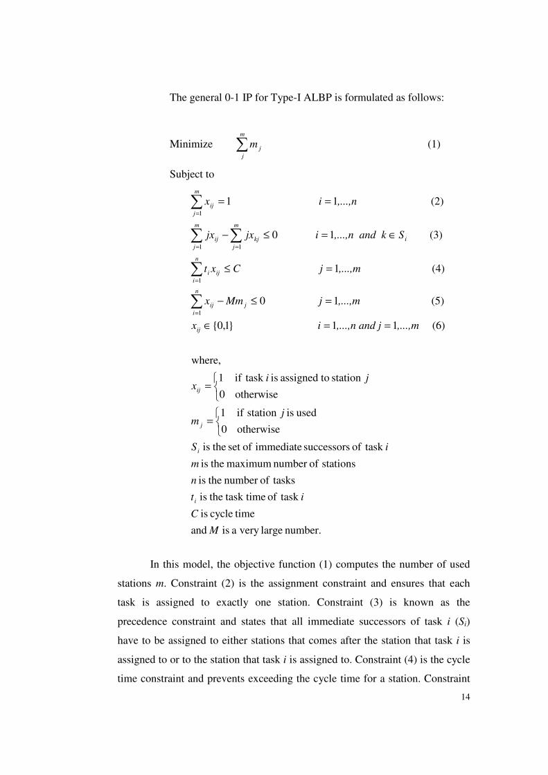
The general 0-1 IP for Type-I ALBP is formulated as follows:
Minimize ∑m
j
jm (1)
Subject to
number. large very a is and
timecycle is
task of task time theis
tasksofnumber theis
stations ofnumber maximum theis
task of successors immediate ofset theis
otherwise0
used is station if1
otherwise0
station toassigned is task if1
where,
(6) 11 }1,0{
(5) 1 0
(4) 1
(3) 1 0
(2) 1 1
1
1
11
1
M
C
it
n
m
iS
jm
jix
,...,m j,...,n andix
,...,mjMmx
,...,mjCxt
Sd k,...,n anijxjx
,...,n ix
i
i
j
ij
ij
j
n
i
ij
n
i
iji
i
m
j
kj
m
j
ij
m
j
ij
=
=
==∈
=≤−
=≤
∈=≤−
==
∑
∑
∑∑
∑
=
=
==
=
In this model, the objective function (1) computes the number of used
stations m. Constraint (2) is the assignment constraint and ensures that each
task is assigned to exactly one station. Constraint (3) is known as the
precedence constraint and states that all immediate successors of task i (Si)
have to be assigned to either stations that comes after the station that task i is
assigned to or to the station that task i is assigned to. Constraint (4) is the cycle
time constraint and prevents exceeding the cycle time for a station. Constraint
15
(5) states that station j is used if any task is assigned to it. Constraint (6) is the
non-divisibility constraint and satisfies that any task can be assigned to a
station as a whole or not.
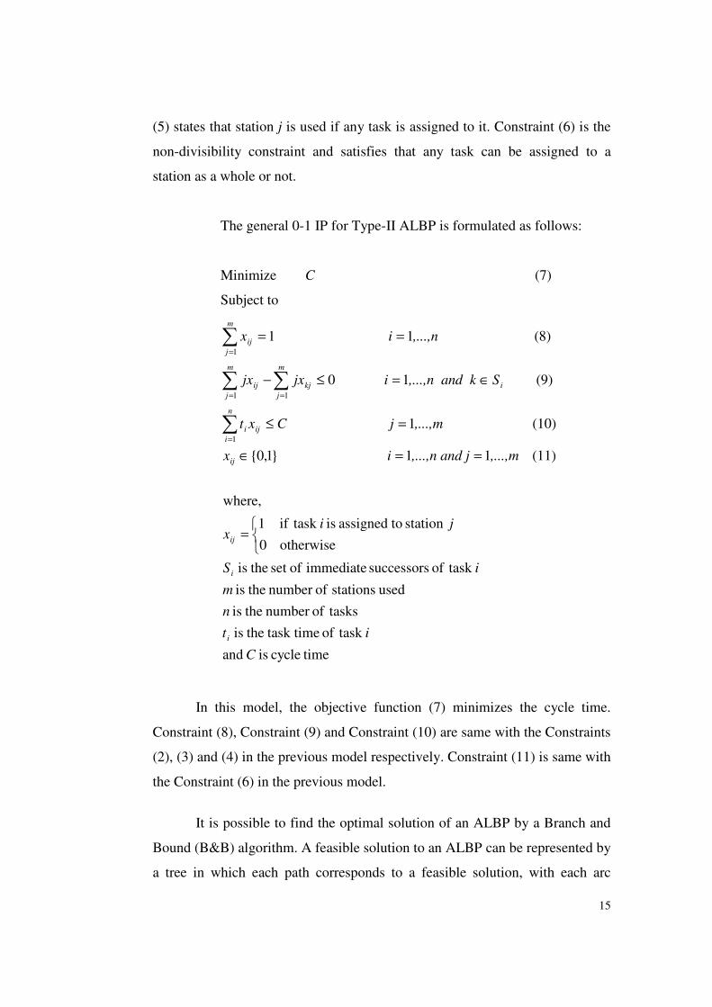
The general 0-1 IP for Type-II ALBP is formulated as follows:
Minimize C (7)
Subject to
timecycle is and
task of task time theis
tasksofnumber theis
used stations ofnumber theis
task of successors immediate ofset theis
otherwise0
station toassigned is task if1
where,
(11) 11 }1,0{
(10) 1
(9) 1 0
(8) 1 1
1
11
1
C
it
n
m
iS
jix
,...,m j,...,n andix
,...,m jCxt
Sd k,...,n anijxjx
,...,n ix
i
i
ij
ij
n
i
iji
i
m
j
kj
m
j
ij
m
j
ij
=
==∈
=≤
∈=≤−
==
∑
∑∑
∑
=
==
=
In this model, the objective function (7) minimizes the cycle time.
Constraint (8), Constraint (9) and Constraint (10) are same with the Constraints
(2), (3) and (4) in the previous model respectively. Constraint (11) is same with
the Constraint (6) in the previous model.
It is possible to find the optimal solution of an ALBP by a Branch and
Bound (B&B) algorithm. A feasible solution to an ALBP can be represented by
a tree in which each path corresponds to a feasible solution, with each arc
16
representing a workstation. Optimal solution can be found by evaluating the
paths enumeratively.
Jackson (1956) presented the first branch and bound algorithm to solve
the ALBP. In this algorithm, before any assignment is made to the last station,
all assignments except for the last station are examined explicitly. Therefore,
the algorithm is time consuming. Jackson (1956) showed that an optimal
solution exists in a full enumeration tree whose arcs represent only maximal
stations. A station is maximal, if no unassigned task can be added feasibly.
Hu (1961) and Mertens (1967) are some of the authors that present
optimum tree-search procedures for solving ALBP in their studies.
Wee and Magazine (1981a) constructed a B&B algorithm. This
enumerative method was formulated for the minimization of the number of
workstations. They developed two heuristics, one of which is a variation of the
bin packing problem and the other is basically a reverse application of the
Ranked Positional Weight Technique due to Helgeson and Birnie (1961).
Wee and Magazine (1981b) developed another B&B algorithm by
modifying the one in Wee and Magazine (1981a). This algorithm was
formulated for the minimization of cycle time. They reported four different
search methods. Two of them are search methods starting with lower and upper
bounds. The others are a "binary search" and a "binary and Fibonacci search"
procedures.
Johnson (1988) developed a B&B algorithm called Fast Algorithm for
Balancing Lines Effectively (FABLE) to solve SALBP-I. Because of the fact
that just one branch in the tree needs to be stored at any one time, the use of
backtracking and re-use of the same computer memory locations allow
minimal and predictable memory space to be used. Constructing the tree as one

17
branch at a time is termed laser search by Johnson (1988). In other words,
FABLE is a depth-first B&B algorithm. In the enumeration stage, eight
fathoming rules are used in order to shorten the search time. Although FABLE
is an effective algorithm it has some limitations. For example, some of the
fathoming rules can not be applied if problem includes zoning restrictions.
Hoffmann (1992) proposed a single solution method called EUREKA.
EUREKA makes depth-first laser search by using "theoretical minimum total
slack time" fathoming rule. Since EUREKA is a depth oriented laser search
algorithm, only the current branch needs to be recalled along with the
precedence information and thus computer storage does not have to be
allocated for alternate nodes. EUREKA uses the procedure that is described by
Hoffmann (1963) to generate a set of tasks for a single station. Hoffmann
Heuristic Technique uses this procedure and creates all alternative task sets for
a single station and selects the set that has the smallest slack time. Then it
passes to the next station. On the other hand, EUREKA uses this procedure to
generate a set for a single station and then algorithm passes to the next station.
As a new station combination is generated, the cumulative sum of station slack
times is calculated. If this sum exceeds the theoretical minimum total slack
time, all emanating branches are fathomed. The algorithm searches in an
orderly manner for an alternative set at this station; if one is found that does not
result in an excessive slack, it goes on to the next station; if not, it backtracks to
the previous station and generates an alternative set of tasks there and
continues. The algorithm continues until all the tasks have been assigned and
the theoretical minimum total slack time has not been exceeded or all branches
have been fathomed. If the algorithm can not find a feasible solution at the end
of searching all the branches, it increases the theoretical minimum number of
workstations by one and the theoretical minimum total slack time by cycle
time, then searches all branches again. When problem size gets larger, it may
take unreasonable time to search all branches. Therefore, Hoffmann sets a time
limit for computation, and if the algorithm can not find a feasible solution at
the end of this time limit, then the algorithm searches in the backward direction
18
in the tree of branches. If the algorithm again can not find a feasible solution at
the end of the time limit, it uses Hoffmann Heuristic Technique (1963) to find
a feasible solution.
Klein and Scholl (1996) developed Simple Assembly Line Balancing
Optimization Method (SALOME). The version of the algorithm that is
developed to solve Type-I ALBP is called SALOME-I. This algorithm is a
multiple solution method that performs bidirectional search. It integrates and
improves the most promising components of FABLE and EUREKA and it uses
some additional bounding and dominance rules. A local lower bound method is
used in each node to dynamically decide on the planning direction. The
branching scheme used is station oriented.
Dynamic programming (DP) is another technique in order to solve
ALBPs optimally. The main problem of all dynamic programming methods is
that the computations required grow at an exponential rate with the increasing
problem size. Jackson (1956) developed the first algorithm based on dynamic
programming (DP) to solve ALBPs. He starts by generating all feasible
assignments to the first station. Then one generates all feasible assignments to
the second station, given the first station assignments. Then, for all feasible
first-second station combination, all feasible assignments are generated for the
third station. The algorithm is then repeated by adding a new station and stops
with the optimal solution (Baybars, 1986).
Held and Karp (1962) reported a new DP algorithm which was
described in detail in Held, Karp and Sharessian (1963). They proposed a
solution method in two parts: first part consists of a dynamic programming
technique for the exact solution of small problems and the second part finds an
approximate solution of large problems by an iterative procedure. Schrage and
Baker (1978) proposed an efficient dynamic programming algorithm. They
19
defined and used feasible subsets of tasks and enumerate all of them with a
labeling scheme.
2.2.1.1.2 Heuristic Solution Approaches
Solving the ALBP optimally can not always be possible because of the
problem size. When the problem size gets larger, solving the problem
optimally becomes harder and even impossible in a reasonable computation
time. Therefore, several heuristic approaches have been tried so far to find a
good solution, maybe the optimal one, but they do not guarantee it, in a
reasonable time.
The Ranked Positional Weight Technique (RPWT), due to Helgeson
and Birnie (1961), is one of the best known heuristic methods proposed. The
procedure constructs a single sequence. A task is prioritized based on the
cumulative assembly time associated with itself and its successors. Tasks are
then assigned in this order to the lowest numbered feasible station (Askin and
Stanridge, 1993).
Hoffmann (1963) proposed the Successive Maximum Element Time
Method (known as Hoffmann heuristic). This method uses precedence matrix
to generate all feasible assignments and aims to make assignment with the least
slack time.
Arcus (1966) presented COMSOAL (Computer Method of Sequencing
Operations for Assembly Lines). Procedure constructs the set of available tasks
that can be assigned to the current station and chooses and assigns any task
from this set randomly. Then it updates the available task set and assigns
another task randomly. The algorithm stops when all tasks are assigned.
Because of this random selection, algorithm gives different solutions at the end

20
of every run. It is a fast algorithm and offers a set of sequences to the
researcher. It is especially useful for large problems.
Raouf and Tsui (1980) proposed Critical Path Approach to solve
SALBP-I. Their method first determines the critical path, then gives priority to
the tasks that are on the critical path while assigning tasks to the stations.
Baybars (1986a) proposed a heuristic method in which he first
eliminates some tasks and reduces the size of the problem. Then he
decomposes the problem into some smaller problems, searches their solutions
and finally combines their solutions to construct the entire solution.
Heckman, Magazine and Wee (1989) developed several heuristic
fathoming rules and proposed a fast and effective branch-and-bound
method.
2.2.1.2 Single-Model Deterministic Type-II ALBP
While a large variety of exact solution procedures exists for Type-I
problem, only few have been developed which directly solve SALBP-II. Most
research has been devoted to search methods which are based on repeatedly
solving SALBP-I.
Helgeson and Birnie (1961) proposed solving Type-II problems, for the
first time, as a sequence of Type-I problems. For any value of cycle time, the
Type-I problem is solved. If the minimum number of stations obtained from
solution of Type-I problem is less than the given number of stations, then the
cycle time is made smaller. If it is more than the specified number of stations,
then the cycle time is made larger. At the end, the minimum cycle time is
found for the given number of stations.
21
Klein and Scholl (1996) proposed a branch and bound algorithm, called
SALOME-II, for the SALBP-II. SALOME-II is the adaptation of SALOME-I
to SALBP-II. It solves Type-II problems by using a new enumeration
technique, the Local Lower Bound Method, which is complemented by a
number of bounding and dominance rules. It makes unidirectional and
bidirectional search.
Uğurdağ, Rachamadugu and Papachristou (1997) presented a two-stage
heuristic procedure to solve SALBP-II. Their approach is based on the integer
formulation of the problem. The first stage, which is based on a heuristic
procedure they have developed, provides an initial solution to the problem. The
second stage improves the initial solution using a simplex like algorithm.
Recently, meta-heuristic approaches became very popular to solve
many different NP-hard combinatorial problems. These brilliant approaches
provide a way to construct efficient heuristic algorithms to solve a specific
problem. It is possible to solve SALBP-I or many other variations of ALBP
like SALBP-II, multi-objective, stochastic, multi/mixed-model, U-type or any
other assembly line balancing problem with these meta-heuristics. Because
these methods are general approaches to solve any kind of ALBP as well as
SALBP, they are discussed in the last section of this chapter.
2.2.2 Mixed-Model ALBP
Mixed-model assembly line is the line on which the simultaneous
production of more than one model is realized. On a mixed-model assembly
line, the lot sizes are usually very small, like one. Although there are numerous
studies published on the various aspects of the line balancing problem, the
number of studies on mixed-model is relatively small. (Gökçen and Erel,
1998).
22
The most important difference between single-model and mixed-model
assembly line balancing (MiALB) is seen in the precedence constraints. In
SALB, there is only one model and precedence diagram. However, in MiALB,
every model has its own precedence diagram and a solution (balance) can not
violate any of these constraints.
The mixed-model assembly lines assume that both changeover times
and changeover costs are negligible. This assumption allows to transform the
problem into single-model assembly line balancing problem. There are mainly
two methods used in this transformation: combined precedence diagram and
adjusted task times. The first approach combines the precedence diagram of the
different models into a single precedence diagram. The second approach is
appropriate only when different models have the same precedence diagram, but
with different task times. The combined precedence diagram method is more
widely used in the literature.
Combined Precedence Diagram Methods
Macaskill (1972) gives the formal definition of combining many single-
models into a single precedence diagram. When the precedence diagram of
model i is represented by a graph Gi=(Vi,Ai), where Vi is the set of tasks of
model i and Ai is the set of precedence relations, the combined graph is
G=(V,A), where V=∪i Vi and A=∪i Ai \{redundant arcs}. An arc (i,j) is
redundant if there exists another path from i to j in G. The mixed-model
defines the number of units to be produced from each model during a shift of T
time units. The processing time of i∈V is equal to the total time required for the
processing of this task in a given mixed-model.
Figure 2.2 illustrates the combined precedence diagram method. The
numbers above each node represent the task time of the corresponding task.
Note that the redundant arcs are indicated with a dashed line.

23
Figure 2.2 A combined precedence diagram constructed from two models
2 4
5 6
7 8
2
5
5 1
1
4
Model 2
Number of units required: 1
1
2
3
4
9
7
6
8
5
10
9 1
1
15
2
2
8
6
1
2
3 6
8
9
2
3
2
5
5
1
Model 1
Number of units required: 2
24
The balancing of the mixed-model line using the combined precedence
diagram approach is similar to the balancing of a single-model assembly line.
The only difference is that the tasks are assigned to the stations on shift, T,
which is the basis in the combined precedence diagram method, instead of the
cycle time, C.
Thomopoulos (1967) was the first researcher who used the combined
precedence diagram to solve MiALBP. Thomopoulos and then Macaskill
(1972) applied heuristics developed to solve SALBP to their combined
precedence diagrams.
Fokkert and de Kok (1997) summarized the advantages and
disadvantages of the combined precedence diagram method. According to their
study, an advantage of this method is that every repetition of a task is
performed by the same workstation, resulting in minimum learning costs. A
disadvantage of this method is related to the balancing on shift basis. Another
model mix can lead to another balance and this might create some confusion on
the shop floor. Another disadvantage of the method is that it might lead to
unequal distribution of the total work content of single-models among the
workstations.
Gökçen and Erel (1998) developed a binary integer programming
model for the MiALBP. They attempt to decrease the size of the model by
using combined predecence diagram and lower and upper bounds that limit the
increase in the number of decision variables and constraints. The results
obtained with their model are significantly superior to the one in the literature
with respect to the number of decision variables and constraints. But the
suggested model is capable of solving problems with up to 40 tasks in the
combined precedence diagram.
Gökçen and Erel (1997) proposed a goal programming approach to
solve MiALBPs with conflicting objectives. They use their mathematical
25
model in 1998 with different objective functions. The goal programming
method they proposed solves the problem with the most important objective.
Then they add the previous solution as a constraint to the model and solve it
with the next objective.
In the study of Erel and Gökçen (1999) a shortest-route formulation of
the mixed-model assembly line balancing problem is presented. Common tasks
across models are assumed to exist and these tasks are performed in the same
stations. The formulation is based on an algorithm which solves the single-
model version of the problem. The mixed-model problem is transformed into a
single-model problem by using combined precedence diagram. They use TST
associated with each model as a performance measure.
Ayral (1999) used combined precedence diagram method to solve the
mixed-model assembly line balancing problem of Arçelik Dishwasher Plant.
She has developed a decision support system. The system provides alternative
solutions to decision makers for single or mixed-model assembly line
balancing problems. The program uses single-model balancing methods
proposed by Wee and Magazine (1981a, 1989) to solve the problem.
Bukchin and Rabinowitch (2006) seek to minimize the sum of costs of
the stations and the task duplication. They develop an optimal solution
procedure based on a backtracking, dept-first B&B algorithm and evaluate its
performance via a large set of experiments. They also propose a B&B based
heuristic for solving large-scale problems.
Adjusted Task Times Method
The second method to transform the MiALBP into SALBP is the
"adjusted task times" method. This method is only useful for the situation that

26
all models have the same precedence diagram, but with different task times.
The method calculates the average task times with the following formula:
ti=Σk fktik
where ti is the average task time of task i, tik is the task time of task i on model
k and fk is the frequency of model k. Frequency of a model is the persentage of
the production of that model in the total production.
Fokkert and de Kok (1997) also summarized the advantages and the
disadvantages of the "adjusted task times" method. Their study suggests that
using the cycle time base, instead of the shift base, is the advantage of this
method. A disadvantage of the method is that there is no procedure which
determines the sequence of models in which they are produced. Another
disadvantage is that this method is not appropriate, if models have different
precedence diagrams, which is a more realistic situation.
2.2.3 Multi-Model ALBP
Multi-model assembly line balancing problem (MuALB) differs from
MiALB in the magnitude of the lot sizes. The problem shifts to MuALBP when
lot sizes get larger. So, changeover costs are important in MuABP. In the
mixed-model assembly line balancing, because the lot sizes are very small,
solution approaches try to balance the line such that tasks would be performed
on the same station for different models. As it is mentioned before, these
procedures may ignore the changeover costs. But in the multi-model assembly
line balancing, although it is not a preferred situation because of the learning
effect costs, it may be preferred to assign a certain task to different stations for
different models. In other words, it may be more appropriate to make more
model specific balancing. In the literature some studies ignore the learning
27
curve effects and make completely separate balancing for different models as
in the case of SALB.
Wild (1972) proposed to balance a multi-model line with the balancing
methods of MiALBP, when the lot sizes are small and carrying out every
repetition of a task at the same station is more beneficial. Moreover, he
suggested to solve MuALBP with successive applications of the solution
methods of SALBP for each model, when the lot sizes are large. He proposed a
heuristic method that starts with balancing the line for the model which has the
biggest production rate and then assigns the tasks for the remaining models
according to this model's balance. The algorithm computes the efficiency of the
balance by using the slack times. Then it repeats the same procedure for the
model which has the second biggest production rate and so on. At the end, the
solution which has the best efficiency is chosen. The next step searches for the
best sequence of the models to be produced by formulating the problem as an
assignment problem so as to minimize the set up cost. The last step is finding
the batch sizes.
Buxey, Slack and Wild (1993) stated that the objective of MuALBP as
the minimization of the production costs which also include the changeover
costs. They suggested that the number of stations and the location of parts and
equipment should be static and common tasks should be allocated to the same
worker and by the manipulation of the cycle time, the balance delay could be
minimized.
Chakravarty and Shtub (1985) presented a method to solve MuALBP
that considers labor, set-up and inventory costs. They assume that the models
are produced in batches which are transported to the next station as a whole
batch. By placing buffers between two adjacent workstations, they allow the
batch sizes to vary between workstations. They use the combined precedence
diagram approach to transform their problem into SALBP.
28
Berger, Bourjolly and Laporte (1992) described a Branch & Bound
algorithm to solve MuALBP which uses the combined precedence diagram and
the depth-first search.
Altekin (1999) developed a method to balance multi-model assembly
lines. The method tries to minimize the number of used stations. The proposed
method includes upper and lower bounds and branch-and bound procedures.
She first constructs the ‘base model’ which is obtained by choosing the
common tasks for each model and balances the line for the base model as a
single-model assembly line by using EUREKA method. Then she generates the
individual balances for each model by using the balance of the base model.
While generating the individual balances the algorithm she proposes satisfies
the feasibility.
2.2.4 Meta-Heuristic Approaches
The most popular meta-heuristic algorithm is the Genetic Algorithm.
These algorithms simulate the genetic processes of biological organisms. The
algorithms use the 'survival of the fittest' principle of the nature. It was first
proposed by Holland (1975). Genetic algorithms run with a solution set called
generation. Each solution is called a chromosome and each solution component
is called a gene. Generation is a set of chromosomes. The algorithm also
simulates the crossover and mutation processes of the biological organisms to
find the solutions and by using these operators, produces the next generation
according to the fitness values of the solutions. The first operator of Genetic
Algorithms is crossover operator. This is an operator that constructs a
chromosome, called offspring, by using two parent chromosomes. Many
problem specific crossover operators may be defined. But two-crossover
operators are more popular. The first one is one-point crossover. There is only
one crossover point at this operator and this point can be selected randomly or
with any other strategy. The offspring is constructed by taking the first part of
the first parent and the second part of the second parent according to this

29
crossover point. The second operator is two-point crossover. With this strategy,
there are two crossover points and offspring is constructed by taking middle
part from one parent and outside parts from the other parent. The second
operator of the Genetic Algorithm is the mutation operator. This operator
generally makes point changes on a chromosome. Changing the number of
stations of a task, corresponding to the gene that the mutation operator effects,
or changing the places of two genes on the chromosome are some examples of
mutation operator. Many problem specific mutation operators may be defined.
The algorithm constructs a new generation from the current one and converges
after some iteration. According to a parent selection strategy, two parents are
chosen, and with the crossover probability, they are exposed to crossover
operator. After crossover operator, with the mutation probability, offsprings are
exposed to mutation operator. Then according to regeneration strategy, the next
generation is generated from the offsprings and parents. Parent selection and
regeneration strategies are user_specified. Hence, lots of strategies can be
developed. One of the widespread strategies is Roulette Wheel Strategy.
According to this strategy, chromosomes are ranked according to their fitness
values. Then selection probabilities are computed by using fitness values. The
algorithm generates a random number, let it be P, from the uniform distribution
between 0 and 1. The chromosome whose P value is between its selection
probabilities is chosen as one of the parents or passes to the next generation.
One of the other parent selection or regeneration strategies is selecting two
chromosomes randomly and comparing their fitness function values and taking
the better chromosome as one of the parents or passing the better one to the
next generation.
Adapting the general Genetic Algorithms approach to the ALBP
involves some difficulties. The first one is representing a solution
appropriately. There are two most general representations: standard encoding
and order encoding.
30
Standard encoding: The chromosome is defined as a vector containing
the labels of the stations to which the tasks 1,...,n are assigned (Scholl and
Becker, 2004).
Order encoding: The chromosomes are defined as precedence feasible
sequences of tasks (Scholl and Becker, 2004).
The other difficulty faced, while constructing Genetic Algorithm to
solve ALBP, is feasibility. There are many relations between genes of a
chromosome. For example, a chromosome has to satisfy: precedence
restrictions, cycle time or number of stations limitations, assignment of all
tasks, representation of each task only once in a chromosome, etc. All of these
relations may cause infeasibilities after crossover or mutation operators. After
these operators, offspring may have a task that is repeated two times or a task
may not be represented or cycle time or precedence relations may be violated.
To overcome these difficulties, a repair algorithm has to be developed or
infeasible solutions have to be penalized.
The best solution is updated and stored while the algorithm is running
and when the algorithm stops, the best solution is obtained.
There are many studies that use GA approaches to solve various
assembly line balancing problems. Some of them are: Anderson and Ferris,
1994; Rubinovitz and Levitin, 1995; Kim, Kim and Kim, 2000; Sabuncuoğlu,
Erel and Tanyer, 2000; Goncalves and Almeida, 2002; Ponnambalam,
Aravindan and Subba Rao, 2003.
Another meta-heuristic approache is Tabu Search, which tries to
improve a given feasible solution by iteratively transforming it into other
feasible solutions. Such transformations are referred to as moves. Solutions
which may be obtained from a given solution S by means of a single move are

31
called neighborhood of S (School and Becker, 2004). The main logic of Tabu
Search is preventing the moves that give the recently searched solutions for a
certain amount of time and thus, searching for new solutions without cycling.
There are some other strategies of Tabu Search approach like intensification
and diversification which are mentioned below.
There are two types of moves for SALBP: shift and swap. They are
explained using the following notations:
LPj : latest station to which a predecessor of task j is currently assigned.
ESj : earliest station to which a successor of task j is currently assigned.
• A shift (j,k1,k2) describes the movement of a task j from station
k1 to station k2 with k1≠k2. This move is feasible if k2 ∈
[LPj,ESj].
• A swap (j1,k1,j2,k2) exchanges tasks j1 and j2, which are not
related to precedence, between different stations k1 and k2. This
move is feasible if the two corresponding shifts (j1,k1,k2) and
(j2,k2,k1) are feasible (Scholl and Becker, 2004).
The Tabu Search approach forbids the attributes of the moves most
recently performed and makes them tabu for a number of iterations TD (tabu
duration) and stores them in a tabu list TL (recency based memory). When a
swap (j1,k1,j2,k2) is performed, the attributes (j1,k1) and (j2,k2) are added to TL
such that removing j1 to k1 and j2 to k2 is temporarily forbidden for TD
iterations (Scholl and Becker, 2004).
Tabu Search algorithm runs by making local search. Sometimes, all
neighborhood of S is searched and the best move or the first improving move
made or any randomly selected move is chosen as the new current solution, if it
is not tabu. Sometimes, the algorithm needs to overwrite a tabu. The criteria
that determine this need are called tabu aspiration criteria. For any current

32
solution S, all of its neighborhood solutions may be tabu. In this situation, in
order to continue searching the algorithm, the oldest tabu is abolished or the
best move in the neighborhood is selected. Occasionally, the algorithm can find
a solution that is the best solution found so far, but one of the tabu attributes
may prevent this move. At this situation the algorithm can abolish that tabu.
The algorithm starts with an initial solution which is created by any
constructive procedure like COMSOAL or RPWT, and stops when the
stopping criteria are satisfied. The stopping criteria may be the number of
iterations or a computational time limit or any convergence measure.
In order to intensify the search in certain regions or to direct the search
into yet unvisited parts of the solution space, a frequency based memory is
used. In this memory, the relative number of iterations and task-station
assignments are stored (denoted as zjk). Several phases of the search are either
used for collecting frequency information, fixing tasks j in a station k where
they have a high zjk value (intensification) or avoiding those tasks j reenter a
station k where they have a high zjk value (diversification) (Scholl and Becker,
2004).
Some of the studies use TS to solve various assembly line balancing
problems are: Chiang, 1998; Pastor, Andres, Duran and Perez, 2002; Lapierre,
Ruiz and Soriano, 2006.
Another well-known and efficient meta-heuristic approach is Simulated
Annealing. This approach simulates the annealing processes of materials on
the decision problems. The main idea of the algorithm is to escape from the
local optima by giving an acceptance chance to inferior solutions as the next
current solution.
Simulated Annealing algorithm starts with an initial solution which is
initiated by any constructive algorithm and makes moves with swaps or shifts.
33
The probability of accepting inferior solutions decreases, if the negative (bad)
difference between the current solution and worse candidate solution increases
or the value of the control parameter t decreases. Where F is a function to
evaluate a solution, the function that gives an acceptance probability of bad
solution is:
Exp(-(F[candidate solution]-F[current solution])/t).
At the beginning of the algorithm, the value of t is higher and it
decreases during the iterations. This is called cooling and this cooling provides
intensification during the procedure. Algorithm initially searches the space
roughly, and as time passes, it focuses on some good solution regions.
Generally, the final value of the control parameter t is used as a termination
criterion.
Some of the studies that use SA to solve line balancing problems are:
Suresh and Sahu, 1994; Bolat, 1997; McMullen and Frazier, 1998; Xiaobo and
Zhou, 1999; Alp, Cercioglu, Tokaylı and Dengiz, 2001; Mendes, Ramos,
Simaria, Vilarinho, (2005).
Another meta-heuristic approach is Ant Colony Optimization. This
approach is one of the most recent approaches and there are fewer studies on
this method than the previously mentioned approaches. This approach
simulates the process that ants search and find the shortest path that goes to
food. Bautista and Pereria (2002) presented an ant colony algorithm to solve
SALBP-1. McMullen and Tarasewich (2003) proposed an ant colony algorithm
for a generalization of SALBP with respect to parallel stations, stochastic task
times, multiple objectives and mixed-model production.

34
CHAPTER 3
THE CASE STUDY
3.1 The Company in the Study
Today’s global competitive market forces the companies to diversify
their products and develop new models. Companies try to enlarge their market
share, or at least, to save it by producing various models that have different
specifications according to their costumer needs. The consumer durables plant
studied is one of the companies that continue their production with different
models. The firm develops new models and produces different models. It also
modifies its standard models according to customer specifications. But the ratio
of these modifications is very small. Recently, the firm produces four main
models with high production amounts; Model1, Model2, Model3 and Model4.
(See Appendix A for sketch of the layout of the assembly line of the firm).
Model1, Model2, Model3 and Model4 comprise approximately
99-100 % of total production. According to the information obtained from the
production planning department: roughly, Model1, Model2, Model3 and
Model4 each has 70%, 15%, 10% and 5% share in total production
respectively. The production amount is 500 units per shift.
3.2 Current Balancing Method and Development of the Proposed
Method
There is no precedence relationships diagram in the firm. Assignments
of tasks to stations are made manually according to personal experiences by

35
trial and error method. Daily production is adjusted according to the production
plans of a number of months. Then, the line is balanced such that it satisfies
this production rate. Batch sizes of the different models, similarities and
common tasks among models and consequently, assembly sequence of the
models are neglected. This situation is similar to balancing the multi-model
line by using combined precedence relationships diagram and obtaining a
unique assignment, as if it is a mixed-model line. The firm even does not have
the combined precedence relationships diagram, but the assignments are made
by taking into account the list of all tasks and omitting the specifications of the
models. Sometimes, with some more trial studies on this unique balance, small
changes related to the models are made.
Production becomes significantly inconsistent at the week that
balancing is made; because of the trial and error method many assignments
violate the precedence relationships and it stops the production. Trials and
adjustments continue till a feasible solution is achieved. This is a major
disadvantage of the current balancing procedure. Rarely, a small amount of a
different model passes throughout the line among other models. But, generally
system works with large batch sizes as a multi-model assembly line. Balancing
the multi-model assembly line as if it is a mixed-model assembly line is
another disadvantage of the current line balancing procedure. Because of the
lack of the objectives which will be mentioned in Chapter 4, the quality of the
solution thus obtained is not known. Furthermore, even it is a great success to
find any feasible solution to such a large problem based on individual
experiences and trial methods. Due to the lack of evaluating functions and
difficulty of the current method, better solutions may not be searched for. This
is another disadvantage of the procedure.
Our study started as a case study. The main intention was obtaining a
good line balance for the assembly line. The firm wanted us to develop such a
program that uses the daily production information and computes the cycle
36
time and balances the line. The firm was not interested in the objectives
explained in Chapter 4 and related costs. The main interest of the firm was
obtaining any feasible solution that fulfills the daily production. The batch
sizes of the different models in the total daily production and differences
among the models as to the processing requirements were not important for the
firm. Namely, the firm wanted us to develop a software that makes the
balancing job that is currently being made manually.
Every assembly line balancing procedure needs a list of the tasks, task
times, precedence relationships and zoning restrictions. The lists of the tasks
and task times have been obtained from the firm. Then we have determined the
precedence relationships and sub-task lists of the models with our observations
and contributions of the workers.
Initially, because the firm wanted us to develop such a program that
produces a unique balance for all models, we have tried to develop integer
programming-based method and find the optimum solution. At the beginning
of the modeling effort, the size of the problem was absolutely large. Although
we have achieved to decrease the problem size significantly with some
manipulations, the running time was still too long.
During the time of construction of the precedence relationships
diagram, we have observed that the production was more suitable for the multi-
model production rather than the mixed-model production. Hence, balancing
the line according to the mixed-model line balancing method was insufficient.
Then we have determined the individual task lists of the models. We have
realized that some other objectives and the sequencing problem should be also
taken into account. Solving the problem with integer programming for all
models and all possible sequences would require extremely long computation
times. In addition, considering different batch sizes, cycle times and cost
37
component combinations, it is almost impossible to solve the whole problem
with integer programming-based methods.
As it is mentioned in the following paragraphs, we have already made
some assumptions and gave up with the overall optimal solution. Because of
these reasons, we have decided to develop a heuristic approach that can find
good solutions in acceptable computational times, few hours, and can be
adapted to different scenarios with different model mix, batch sizes, objective
weights, etc.. The proposed approach and the relevant code are explained in the
following chapter. The problem is explained in the following parts of this
chapter.
3.3 Determining the Problem
3.3.1 Tasks
The first step is to determine the tasks and to construct the list of tasks.
Any task consists of some sub-operations. For example, in order to perform a
task, we may take a part from a specific location, do some operations on that
part and then assemble it into the main part. Sometimes, it may be very
difficult to determine the bounds of the task. If tasks are defined such that they
consist of many operations, this may cause a task to be defined as aggregation
of tasks. As a result, this situation dictates any solution to assign this group of
tasks to the same station. It shrinks the solution space and may exclude the
optimum solution. On the other hand, defining a task such that it includes very
few operations may cause infeasibility. For instance, some sub-parts of a given
task may be defined as separate tasks. Hence, sub-parts of a task may be
assigned to different stations which results in infeasible solutions. In
conclusion, tasks have to be defined such that they are not groups of tasks or
sub-parts of a specific task.

38
In our study, tasks were already defined in the firm. We have got these
definitions, but it was difficult to observe production and identify these tasks.
While we try to construct precedence relationships diagram according to this
task list, we have realized that there were some mistakes in this list. There were
some tasks in the list which were already abolished. In contrast, there were
some tasks that we have observed on the line but missing in the list.
Sometimes, a task was performed more than once on the line, but coded and
named once in the list. In order to balance any line, all tasks that have to be
done on that line must be known. If any task is repeated more than once, every
repetition may have the same name, but each of them must have different
codes. By discussing these situations with workers, we have adjusted the task
list. There were some other undefined tasks which were being performed
automatically by robots. Because we have needed them in the precedence
relationships diagram, we have defined and coded them. Then we have
distinguished the task list for each model. Task lists are given in Appendix B.
There is a task “Oil the reel of hinge” in the list which is repeated two
times on the line. It is adjusted by defining two separate tasks “Oil the right
reel of hinge” and “Oil the left reel of hinge” (task 7 and task 27). There are
some automatically made tasks which are defined as “Erect the main part”,
“Functional test” and “Fill water to the salt box” (Tasks 72, 289 and 310).
Many others are similarly added or removed to/from the list by discussing with
the workers and the list is updated.
3.3.2 Task Times
Next step is determining the task times. Actually, it requires a lot of
observations, measures, some statistical and analytical computations and
goodness of fit tests, etc.. However, task times were obtained from the firm.
Since no other task can be assigned to the stations of newly defined and
39
automatically performed tasks, the task times of these tasks are taken as cycle
time. Task times are given in Appendix B.
There were some zoning restrictions due to which it was impossible to
assign any other task to the same station with these tasks. To prevent infeasible
assignments, task times of these special tasks were taken as being equal to C.
These tasks are task 72, task 195, task 259, task 289, task 310 and task 317.
3.3.3 Precedence Relationships Diagram
The most difficult step of the case study was to build the precedence
relationships diagram. There were lots of alternative diagrams. It was a
demanding work to represent the real situation on the paper. Occasionally, we
were to make some assumptions and decisions. On the other hand, we were
trying to represent the real situation as much as possible with minimal essential
assumptions.
While we were trying to construct the diagram, we have realized that it
was not obligatory to perform all of the listed tasks on the line. There were a
lot of tasks which could be performed off the line. This relaxation gives rise to
thousands of alternative precedence relationships diagrams. It messed up our
studies up to that point. We faced with a lot of questions and decisions like;
� Which tasks were to be made on the line?
� Which tasks could be performed off the line?
� If we had determined all of these tasks and extracted them from the
list, what would have happened?
� Since extracting all of these tasks from the line messes up the real
situation, which subsets of these tasks should be extracted?
� What were the advantages and disadvantages of the decision about
extracting tasks from the line?
40
When we consider all of the subsets of these tasks, there are thousands
of alternative precedence diagrams and consequently, thousands of alternative
solutions. Since we were trying to solve this real life problem and find the best
solution, each of these alternatives was an alternative applicable solution.
Finally, since the advantages and disadvantages of the alternative
solutions are not known, we have decided to consider only the current situation
of the line; we have decided to assume that all tasks being performed on the
line currently have to be performed on the line.
The other important and difficult decision was about the tasks that
require opening and closing the lid of the machine (product). There are two
tasks as, “Open the lid” and “Close the lid”. There is a code for “Open the lid”
and another one for “Close the lid”. But on the line, each of them is repeated
more than once. In order to balance the line, we have to know exactly how
many tasks we assign to the stations, the relationships between them, the task
times and the zoning restrictions. But at almost every step of our observations,
we have faced with very flexible situations. There are some tasks which have
to be performed inside the machine. Let us consider two of them. It is possible
to assign one of them to a station and the other one to another station, or it may
be possible to assign them to the same station according to the precedence
relationships. If these two tasks are assigned to different stations, there would
be two alternative situations. In the first case, a pair of “Open the lid”, “Close
the lid” tasks would be also assigned to each of the stations and those two tasks
would be performed on the machine. This situation requires two “Open the lid”
and two “Close the lid” tasks. In the second case, the lid is opened at the first
station, the first task is performed, the machine moves to the second station
with the open lid, the second task is performed and then the lid is closed. This
situation requires one “Open the lid” and one “Close the lid” tasks. But this
time if we allow moving the machine with the open lid between stations, the
“Open the lid” task may be assigned to a previous station of the first station
41
and the “Close the lid” task may be assigned to a successor station of the
second station. At this point some other questions may arise; “Is it feasible to
move the machine with the open lid between stations?”, “If it is infeasible for
some stations, what will happen?”, “Sometimes the open lid forces the worker
to go away from the machine and gets the work harder, how will the moves
with the open lid affect the production?”, etc. If these two tasks are assigned to
the same station, it is needed to assign one “Open the lid” task and one “Close
the lid” task to this station. In the real problem, there are 38 such tasks and it is
possible to attain thousands of different alternative precedence diagrams.
Increasing the number of “Open the lid”-“Close the lid” pairs and
decreasing the number of inside-tasks between each pair on the precedence
relationships diagram enlarges the solution space and gives a chance to find
better solutions. But at the same time, it increases the number of tasks, work
content, number of stations and most importantly the size of the problem.
Decreasing the number of “Open the lid”-“Close the lid” pairs and increasing
the number of inside-tasks between each pair on the precedence relationships
diagram decreases the work content and problem size, but it shrinks the
solution space and may lead to worse solutions. It was impossible to construct
all possible precedence relationships diagrams and solve the problem overall
alternatives. We were to choose one of them. Thus, we decided to give up the
overall optimum solution. Instead, we chose to find the best possible solution.
There are some zoning restrictions and tasks that have to be assigned to the
same station. One of the groups of these tasks (317 TASK GROUP 4) has a
total task time of 43.3 seconds. By considering this situation, we have grouped
the inside-machine tasks such that their total task time can not exceed 30-35
seconds. According to these groups we have added “Open the lid”-“Close the
lid” pairs. The selection procedure is a heuristic approach, but we have tried to
save the flexible structure and represent the current production line as realistic
as possible. The final task list is given in Appendix B. Precedence relationships
42
for individual models are given in Table C.1 and combined precedence
diagram is given in Figure C.1 in Appendix C.
3.3.4 Zoning Restrictions
In addition to precedence relationships, zoning restrictions specify some
special restrictions. Because of the requirement of some special equipment, a
task can be performed at only some specific stations. Occasionally, it can be
neccessary to perform some specific tasks together at the same station or
separately at different stations. Such limitations are called zoning restrictions.
We have determined many zoning restrictions at the assembly of consumer
durables in the firm. Sometimes we have represented them in the precedence
diagram or we have manipulated the task times so as to satisfy these zoning
restrictions or we have used them in the file which consists of the station
numbers at which a task may be performed (assignable station numbers).
There is a robot and special equipment at station 11. Tasks 12, 15, 16,
18 and 20 are to be performed at this station because of this special equipment.
Because of the precedence relationships, tasks 13, 14 and 17 are to be assigned
to station 11. Since the worker at station 11 can handle many tasks, it is
feasible to assign other tasks to station 11. Furthermore, since the worker does
tasks 13, 14 and 17, while the robot turns the pallet, the task times of task 12
and task 20 are defined as zero. Assignable station numbers are fixed to 11 for
tasks 12, 13, 14, 15, 16, 17, 18 and 20.
There is another robot at station 17 which changes the position of the
machine. It holds and lifts the machine. Then, it turns the machine and puts it
again on the pallet. There is no worker at this station. Hence, it is impossible to
assign some other tasks to station 17. The robot can only perform task 72. The
task time of task 72 is taken as cycle time and the assignable station number is
fixed as 17 for task 72.
43
Task 310 is performed by a robot automatically at station 22. Task time
of task 310 is taken as the cycle time and the assignable station number is fixed
as 22 for this task. Similarly, task 195 is performed by a robot automatically at
station 43. Task time of task 195 is taken as the cycle time and the assignable
station number is fixed as 43 for this task.
Tasks 207, 210, 211, 212 and 216 are to be done at station 44, because
of another robot. Likewise, because of the precedence relationships, tasks 208
and 209 are assigned to station 44. There is a worker at the station and it is
possible to assign some other tasks to this station. Since the worker performs
tasks 208 and 209 while the robot works, their task times are defined as zero on
the line. Assignable station numbers are fixed as 44 for these tasks.
There is a parallel station (station 29) to the line and tasks 298, 299,
300, 301, 302, 303, 304, 305, 306, 307, 308, 309 and 311 are to be performed
at this station because of a specific equipment: fixture.
Tasks 173 and 178 are to be done at the same station. This situation first
is represented by taking each of them as a predecessor and the other as a
successor. But after developing the proposed meta-heuristic algorithm, since
this situation is preventing the running of the algorithm, tasks 173 and 178 are
taken as one combined task (323 TASK GROUP 10).
Tasks 275 and 280 are to be performed at the same station. Because of
the precedence relationships, tasks 272, 273, 274, 279 are also to be assigned to
the same station. This restriction is satisfied by adding the arc (280,275) to the
precedence relationships diagram.
There is a special section on the line. This section includes stations 45,
46, 47 and 48. There is much space to put the product (machine). There are
workers at these stations who set the machine and test it. A machine works as a
44
finished item. If there is a problem, the machine is sent to the repair
department. This section is dedicated to test operations only. In order to
represent this situation in the precedence diagram, we have defined a task
(functional test) and give a code (289). Then we have taken its task time as the
cycle time and fixed the assignable station number as 45. The task “289 test” is
always assigned to station 45, but it shows that test is made at one of the
stations 45, 46, 47, 48. For other tasks, these stations are removed from the
assignable station numbers in order to prevent assigning any other task to these
stations.
There is a parallel sub-assembly line to the assembly of the inner lid. A
conveyor moves an inner lid and a worker takes this inner lid and assembles it
to the main part. The task 86 is to be assigned to station 23. By using
assignable station numbers and fixing it as 23 for task 86, this zoning
restriction is integrated into the algorithm.
Similarly, task 259 is to be performed by a robot automatically at
station 54. Task time of task 259 is taken as the cycle time and assignable
station number is fixed as 54 for this task.
Since it is not allowed to move a machine between stations with the
open lid, a pair of “Open the lid”-“Close the lid” tasks has to be assigned to the
same station. If this is the case, the tasks which are in between this pair in the
precedence relationships diagram have to be assigned to the same station.
According to this result, tasks 106, 199, 200, 201, 202, 203 and 189 have to be
assigned to the same station. Tasks 190, 252, 253, 255, 261, 262, 263, 264,
256, 254, 257, 258, 265 and 194 have to be assigned to the same station.
Similarly, tasks 312, 281, 282, 283 and 313; tasks 160, 284, 290, 285, 286,
288, 296, 161, 287, 291 and 292; tasks 217, 218, 219, 220, 222, 223, 224, 225,
226, 227 and 228 have to be assigned to the same stations. Because an
45
equipment performs task 219 while the worker is doing some other tasks, task
times of tasks 220 and 223 are defined as zero on the line.
3.4 Integer Programming Studies
At the beginning of the studies with integer programming, the problem
size is found to be absolutely large. There are 313 tasks at the combined
precedence diagram and 68 stations on the line which is equivalent to
(68)(313)=21284 binary decision variables in the mathematical model. The
main models of the product (Model 1, 2, 3 and 4) consist of 270, 271, 282 and
297 tasks, respectively. Hence, there are approximately 18360 to 20196
(=(68)(270) to (68)(297)) binary decision variables in the individual
mathematical models of the individual product models. We have used the
precedence relationships and zoning restrictions, and made the following
manipulations to reduce the problem size:
� There are 6 tasks which have task times equal to the cycle time
(tasks 72, 195, 259, 289, 310 and 317). Since the assignment of any other task
to the same stations with these tasks is impossible, we have discarded
assignment variables of other tasks to these stations. We have also discarded
assignment variables of all tasks to stations 46, 47, 48 because of task “289
functional test”. These operations decrease the number of binary variables
approximately by 2700 (=(6+3)(300)) for roughly 300 tasks.
� Since tasks 72, 195, 259, 289, 310 and 317 are to be assigned to the
specific stations, it is possible to remove the assignment variables of these
tasks to other stations. This process reduces the number of binary variables by
402 (=(68-1)(6)).
46
� Some tasks between a pair of “Open the lid”-“Close the lid” are to
be assigned to the same station with that pair. So, it is possible to group these
tasks and assume them as one task.
• Tasks 106, 199, 200, 201, 202, 203 and 189 are combined and
called as “315 TASK GROUP 2”. This reduces the number of
variables by 408 (=(7-1)(68)).
• Tasks 12, 13, 14, 15, 16, 17, 18 and 20 are combined and called
as “314 TASK GROUP 1”. It reduces the number of variables
by 476 (=(8-1)(68)).
• Tasks 207, 208, 209, 210, 211, 212 and 216 are combined and
called as “316 TASK GROUP 3”. It reduces the number of
variables by 408 (=(7-1)(68)).
• Tasks 298, 299, 300, 301, 302, 303, 304, 305, 306, 307, 308,
309 and 311 are combined and called as “317 TASK GROUP
4”. It reduces the number of variables by 816 (=(13-1)(68)).
• Tasks 275, 272, 273, 274, 279 and 280 are combined and called
as “318 TASK GROUP 5”. It reduces the number of variables
by 340 (=(6-1)(68)).
• Tasks 190, 252, 253, 255, 261, 262, 263, 264, 256, 254, 257,
258, 265 and 194 are combined and called as “319 TASK
GROUP 6”. It reduces the number of variables by 884
(=(14-1)(68)).
• Tasks 312, 281, 282, 283 and 313 are combined and called as
“320 TASK GROUP 7”. It reduces the number of variables by
272 (=(5-1)(68)).
• Tasks 160, 284, 290, 285, 286, 288, 296, 161, 287, 291 and 292
are combined and called as “321 TASK GROUP 8”. It reduces
the number of variables by 680 (=(11-1)(68)).
• Tasks 217, 218, 219, 220, 222, 223, 224, 225, 226, 227 and 228
are combined and called as “322 TASK GROUP 9”. It reduces
the number of variables by 680 (=(11-1)(68)).

47
• Tasks 173 and 178 are combined and called as “323 TASK
GROUP 10”. It reduces the number of variables by 68
(=(2-1)(68)).
� After these preliminary studies, the number of binary variables is
reduced by approximately 50% (by 8000 to10000 variables). But the number of
variables is still high to try to solve the problem optimally. It is possible to use
precedence relationships and zoning restrictions to reduce this number further.
For example, task 72 is to be assigned to station 11. If that is the case, no one
of the preceding tasks of task 72 at precedence relationships diagram can be
assigned to the successor stations of station 11. By using precedence
relationships, task times, a pre-determined cycle time and zoning restrictions,
we have found the upper and lower bounds of stations that a given task may be
assigned to for each of the tasks. Then we have removed the unnecessary
assignment variables.
The number of assignment variables is reduced to approximately 2000.
Then we have constructed the mathematical model IP formulation of which is
given in Chapter 2 for each machine type for a given cycle time and searched
the minimum number of stations. We have used LINGO 8.0 and CPLEX 8.1
programs, but still the running times were very high; more than a day for one
product model. We have stopped the runs without achieving any solution. For
four product models, there are 24 possible sequences. To evaluate a sequence,
a model has to be constructed and solved for each of the four product models.
To evaluate all sequences for a specific cycle time, it is necessary to construct
and solve 96 mathematical programming models. Considering different cycle
times, different cost components and different batch sizes, it is concluded that
mathematical models can not be used to solve this problem.
In general, in today’s production environment, companies produce
more than one type of a product. The companies that benefit from the assembly

48
lines use the same line to produce different product models. According to our
limited observations, these lines do not consist of a few number of tasks.
Furthermore, almost everything is flexible and consists of many decision
criteria in the real life production processes. Hence, it is very important to be
able to evaluate different situations according to different objective function
combinations and find good solutions in acceptable times, even if it is possible
to find the optimum solution. In this study, a heuristic solution algorithm is
developed to find good solutions in reasonable times for especially
multi/mixed-model. Our algorithm is used to solve such a real life problem
which can be defined as a large-size assembly line balancing problem,
consisting of flexible and multi-criteria real life environment. The proposed
algorithm is explained in detail in the following chapter.
49
CHAPTER 4
THE PROPOSED APPROACH
4.1 Simulated Annealing (SA)
Simulated Annealing is a well-known and efficient meta-heuristic
approach. This approach simulates the annealing processes of materials on the
decision problems. The main idea of the algorithm is to give a chance to the
inferior solutions to be accepted as the next current solution in order to escape
from the local optimums.
Simulated Annealing algorithm starts with an initial solution which is
constructed with any constructive algorithm. At any iteration, the algorithm
generates a neighboring solution by making a randomly chosen small variation
on the current solution. Generating a neighboring solution by making small
perturbations on the current solution provides a way to make detailed search on
the special regions of the solution space. If the candidate solution is generated
by making many changes on the current solution, the algorithm jumps from the
current solution to any other solution residing in a very different region of the
solution space. Thus, using a near neighboring solution as a candidate solution
improves the algorithm performance.
At any iteration, if the candidate solution is better than the current one,
a move to the candidate solution is made. However, if the candidate does not
improve the current solution, the algorithm may adopt the candidate solution as
the next current solution with some acceptance probability or reject it. If the
50
transition from the current solution to the candidate solution is rejected, another
solution in the neighborhood of the current solution is generated and evaluated.
The probability of accepting a poor solution decreases if the negative
(bad) difference between the current solution and worse candidate solution
increases or the value of the control parameter t, which denotes the
temperature, decreases. The function that gives an acceptance probability of a
bad solution is,
Exp (-(F [candidate solution]-F [current solution])/t)
where F is a function to evaluate a solution.
At the beginning of the algorithm, the value of t is higher and it
decreases during the search according to a function known as the cooling
schedule. This cooling provides intensification during the time. Because of the
higher value of t, initially the algorithm searches the space roughly and as time
passes, because of the cooling effect, it focuses on some good solution regions.
If the initial value of the parameter t is chosen very small, the algorithm
cannot escape from the local proximity of the initial solution and approximates
to a local optimal solution in this region. On the other hand, choosing a very
high initial value of t causes a long extended search before starting to intensify
on good regions. Figure 4.1 and Figure 4.2 show examples for the convergence
of the simulated annealing algorithm with a very small and a very high initial
temperature, respectively.
The algorithm stops when the termination criterion is satisfied. Number
of the iterations, the running time or the final value of the control parameter t
can be used as the termination criterion.
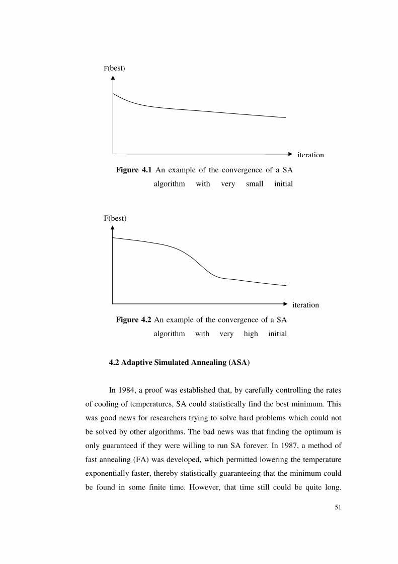
51
4.2 Adaptive Simulated Annealing (ASA)
In 1984, a proof was established that, by carefully controlling the rates
of cooling of temperatures, SA could statistically find the best minimum. This
was good news for researchers trying to solve hard problems which could not
be solved by other algorithms. The bad news was that finding the optimum is
only guaranteed if they were willing to run SA forever. In 1987, a method of
fast annealing (FA) was developed, which permitted lowering the temperature
exponentially faster, thereby statistically guaranteeing that the minimum could
be found in some finite time. However, that time still could be quite long.
iteration
F(best)
Figure 4.1 An example of the convergence of a SA
algorithm with very small initial
iteration
F(best)
Figure 4.2 An example of the convergence of a SA
algorithm with very high initial
52
Shortly thereafter, in 1987, L. Ingber developed Very Fast Simulated Re-
annealing (VFSR) which is exponentially faster than FA. The main idea of the
method was generating the new solution and balancing the temperature by
using the information obtained during the search. The original method was
especially useful for D-dimensional, continuous solution space problems where
one component of the solution is independent from the other components. The
method was affecting the direction of search and the step sizes in each
dimension by evaluating the changes on the objective function values of the old
and the new solutions. Then the temperature was being changed by using the
best solution found so far and the last accepted solution. The original method
was not applicable to all kinds of problems with the original structure. But the
idea of adjusting the algorithm according to the search history pioneered to the
development of ASA. Then the ASA approach was applied to many different
problems (Ingber, 1998; Chen, Istepanian and Luk, 2001).
The temperature change mechanism is an important part of the
transition probability equation. In conventional simulated annealing, the search
begins with a high temperature allowing a higher chance of transition to an
inferior solution. By doing so, the search is able to move out of local minima.
However, as the search continues, the temperature continuously decreases
resulting in a reduced chance of uphill transition. Such an approach could be
useful if the local minima are near the starting point, but may not lead to a near
optimal solution if some local minima are encountered at a relatively low
temperature toward the end of the search. Instead of this monotonically non-
increasing cooling schedule, ASA approach allows adjustment of the
temperature dynamically based on the profile of the search path. Such
adjustments could be in any direction including the possibility of reheating.
Because of these adjustments, the algorithm is not completely dependent on the
initial solution and the initial temperature; the algorithm balances the parameter
itself. Nevertheless, it could be affected from the initial values. Figure 4.3
shows an example of the convergence of an ASA. Figure 4.4 and Figure 4.5
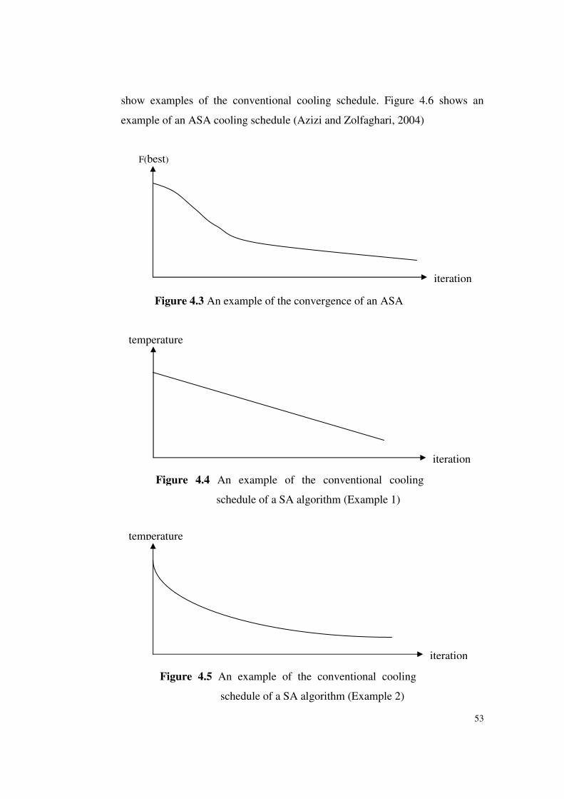
53
show examples of the conventional cooling schedule. Figure 4.6 shows an
example of an ASA cooling schedule (Azizi and Zolfaghari, 2004)
iteration
F(best)
Figure 4.3 An example of the convergence of an ASA
iteration
temperature
Figure 4.4 An example of the conventional cooling
schedule of a SA algorithm (Example 1)
iteration
temperature
Figure 4.5 An example of the conventional cooling
schedule of a SA algorithm (Example 2)

54
4.3 Construction of the Solutions
The majority of the constructive procedures are based on priority rules,
others are restricted to enumerative procedures (Scholl and Becker, 2004).
Restricted enumerative procedures are generally based on the exact
enumeration techniques, which are modified by restricting the search space in a
heuristic manner. Each B&B (or DP) procedure can be applied as a heuristic by
adding heuristic fathoming rules or imposing a time limit. All these procedures
together with the Heuristic of Hoffmann (1963) and its modifications can be
examples of the restricted enumerative procedures.
There are two construction schemes relevant to the priority rule based
approaches. They differ with respect to the manner in which the tasks to be
assigned are selected out of the set of available tasks.
• Station-oriented procedures. They start with the first station
(k=1). The following stations are considered successively. In
each iteration, a task with highest priority which is assignable to
the current station k is selected and assigned. When station k is
iteration
temperature
Figure 4.6 An example of the cooling schedule of an
ASA algorithm

55
loaded maximally, it is closed, and the next station k+1 is
opened (Scholl and Becker, 2004).
• Task (Operation)-oriented procedures. Among all available
tasks, one with the highest priority is chosen and assigned to the
earliest station to which it is assignable (Scholl and Becker,
2004).
The priority rule based approaches use any one of the construction
scheme and work, generally, uni-directionally in forward direction and
construct a single feasible solution. But there are many techniques that work in
backward direction, or flexible bi-direction.
4.4 Representation of the Solutions
There are two most general representations: standard encoding and
order encoding.
Standard encoding: The solution is defined as a vector containing the
labels of the stations to which the tasks 1,...,n are assigned
Order encoding: The solutions are defined as precedence feasible
sequences of tasks (Scholl and Becker, 2004). Numbers of stations that tasks
are assigned to and the station times are computed by adding task times until
the station time of current station exceeds the cycle time. If the station time
exceeds the cycle time by adding the current task to the current station, the next
station is opened and that task is assigned to the next station. An illustrative
example is given below.
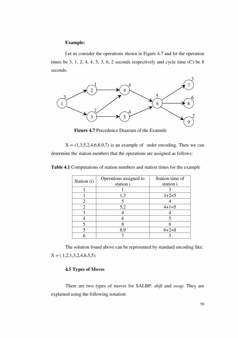
56
Example:
Let us consider the operations shown in Figure 4.7 and let the operation
times be 3, 1, 2, 4, 4, 5, 3, 6, 2 seconds respectively and cycle time (C) be 8
seconds.
X = (1,3,5,2,4,6,8,9,7) is an example of order encoding. Then we can
determine the station numbers that the operations are assigned as follows:
Table 4.1 Computations of station numbers and station times for the example
Station (i) Operations assigned to
station i
Station time of
station i
1 1 3
1 1,3 3+2=5
2 5 4
2 5,2 4+1=5
3 4 4
4 6 5
5 8 6
5 8,9 6+2=8
6 7 3
The solution found above can be represented by standard encoding like;
X = ( 1,2,1,3,2,4,6,5,5).
4.5 Types of Moves
There are two types of moves for SALBP: shift and swap. They are
explained using the following notation:
6 1
2
3 5
4 7
8
9
Figure 4.7 Precedence Diagram of the Example
4
2
1
3
3
4
5
2
6
57
LPj : latest station to which a predecessor of task j is currently assigned.
ESj : earliest station to which a successor of task j is currently assigned.
• A shift (j,k1,k2) describes the movement of a task j from station
k1 to station k2 with k1≠k2. This move is feasible if k2 ∈ [LPj,ESj]
(Scholl and Becker, 2004).
• A swap (j1,k1,j2,k2) exchanges tasks j1 and j2, which are not
related to precedence, between different stations k1 and k2. This
move is feasible if the two corresponding shifts (j1,k1,k2) and
(j2,k2,k1) are feasible (Scholl and Becker, 2004).
4.6 Objectives of ALBP and Evaluation of Solutions
4.6.1 Minimization of the Number of Stations
It is the best known and the most studied objective of the assembly line
balancing problem. Assembly line type production and assembly line balancing
problems are transformed from the simple types (single-model, deterministic
etc. ) to the complicated types (multi/mixed-model, stochastic, parallel, U type,
S type etc.) in the course of time. At the single-model assembly lines,
achieving a pre-determined amount of production with the minimum number of
stations, saves the system from all the costs related to the unused stations
permanently. Consequently, at the single-model assembly lines, minimizing the
number of stations may be the first objective without any other challenging
objectives. On the other hand, assembly lines with the multi/mixed models,
having an unused station at any model’s production, does not save the system
from all the costs related to that station permanently, it saves the system from
these costs at only that model’s production period. In this situation, there may
be any other challenging objective and using that station with a high station
slack time may be preferred to getting that station unused at that model’s
production period.
58
Because the system avoids the costs of unused stations while that model
is produced, minimizing the number of stations must be more important for the
models that have large batch sizes. The component used to evaluate the
solutions according to their number of stations is:
F1[x]=(m1)(Batch Size)(Cycle Time)(Number of Stations)
where x is a solution (line balance) for the model.
The time that is equal to the multiplication of cycle time and the
number of stations is the assembly time and it is equal to the maximum time
allowed to complete a unit product. ((Batch Size)(Cycle Time)(Number of
Stations)) is equal to the total assembly time to complete the batch size units of
products of a model. Here, m1 is the cost of using a station for a unit time. The
batch size and cycle time are constant. This component represents the total
assembly cost of a model. So, if a move decreases the number of stations by
one, it improves the solution by the total cost of using that station in the
production of that model.
4.6.2 Minimization of Cycle Time
This is the second best known objective for assembly line balancing. If
it is certain that the production is to be made with any number of stations, it is
desired to achieve the most frequent production with these stations. It increases
the daily production. Because of the production plan, even it is not wanted to
increase the daily production, minimizing the cycle time decreases the total
production time and the production cost. Furthermore, it provides opportunity
to tolerate some simple problems that may arise during production. Producing
any product with smaller cycle times makes the system more flexible for the
production of other products, if it is necessary to increase the cycle time. Due
to these reasons, if it becomes certain that production is to be made with any

59
number of stations, minimizing cycle time arises as a second objective. The
component used to evaluate the solutions according to their cycle times is:
F2[x]=(m1)(Batch Size)(Cycle Time)(Number of Stations)
Here, m1 is again the cost of using a station for a unit time and the
batch size is constant as well as the number of stations. Because this
component shows the total assembly cost of a model, if any solution decreases
the cycle time by one unit, it saves all stations from this cost for the whole
batch size.
4.6.3 Maximization of Irregularity between Station Times
In general, meta-heuristic approaches search the space by passing from
a current solution to a candidate solution which is generated from the current
solution by making small changes. Simulated Annealing algorithm moves to
the candidate solution if it has a better objective function value. Otherwise, it
passes to the given candidate solution according to the acceptance probability.
Hence, correct evaluation of solutions is very important. If the objective
function uses only the number of stations while evaluating the solutions, all
candidate solutions that have the same number of stations with the current
solution have the same objective function value; however, the objective
function value must decrease by the moves which try to get any station empty.
Because the aim is minimization of the number of stations, the objective
function must encourage these moves by reducing its value. An illustrative
example is given below:
Example:
Let there be an assembly line that has 10 tasks; a, b, c, d, e, f, g, h, i, k.
There is no precedence restriction, all task times are 5 seconds and cycle time
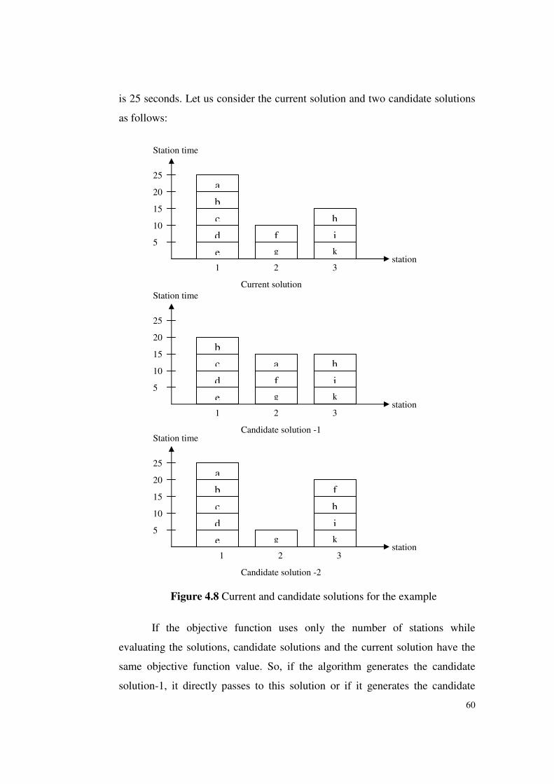
60
is 25 seconds. Let us consider the current solution and two candidate solutions
as follows:
Figure 4.8 Current and candidate solutions for the example
If the objective function uses only the number of stations while
evaluating the solutions, candidate solutions and the current solution have the
same objective function value. So, if the algorithm generates the candidate
solution-1, it directly passes to this solution or if it generates the candidate
2 1 3
a
b
c
d
e g
f
k
i
h
station
Station time
25
20
15
10
5
Current solution
a
b
c
d
e g
f
k
i
h
station
Station time
25
20
15
10
5
Candidate solution -1
1 2 3
a
b
c
d
e g
f
k
i
h
station
Station time
25
20
15
10
5
Candidate solution -2
1 2 3
61
solution-2, it again directly passes to this solution. The candidate solution-1
makes decreasing the number of stations harder. On the other hand, the
candidate solution-2 makes decreasing the number of stations easier. In this
case, the algorithm should understand that the candidate solution-1 is worse
than the current one and penalize this move by increasing its objective function
value. It should also realize that the candidate solution-2 is better than the
current one and encourage this move by decreasing its objective function value.
To achieve this, the following cost component of the objective function is
developed:
Since the SA algorithms search the solution space by passing from a
solution to its neighboring solution, using only the number of stations as an
objective function is not enough to evaluate the solutions to minimize the
number of stations. Maximization of variance (irregularity) in station times is a
sub-objective to achieve the minimization of the number of stations.
4.6.4 Maximization of Smoothness between Station Times
If the stations that are to be used in the production are determined, it is
required to minimize the deviations between the workloads of these stations. In
other words, it is desired to maximize the smoothness between these stations’
workloads. If the deviations among stations’ workloads are high, some stations
are highly loaded, while some of them work at low levels. In this situation,
some of the employees work continuously and some of them have a lot of idle
time. This may cause some satisfaction problems, that is bottleneck station. On
the other hand, the stations that have high workload become more critical. Any
problem occurring in these stations may affect the whole line. Therefore, when
penalty a is 2 andstation used ofset theis where
23
mK
C-WC)(m[x]FKi
i∑∈∀
=

62
the stations that are to be used are known, total workload is required to be
shared equally by these stations as much as possible.
At the previous parts, the cycle time minimization objective is
explained. For the meta-heuristic approaches, as it is a sub-objective to
maximize irregularity to achieve minimization of the number of stations,
maximization of smoothness is a sub-objective to achieve minimization of
cycle time. Determination of the stations that will be used in production means
having a line balance that the production quantities can be met. After having
such a balance, it is required to minimize the cycle time and maximize
smoothness to improve this balance. In order to minimize the cycle time, if the
objective function only uses cycle time, it could not be enough to evaluate the
solutions truly. There should be such an objective function component that
encourages the moves which transfer a task from a station that has high station
work content to a station that has low station work content and punish the
reverse moves. The component developed to achieve this is given below:
4.6.5 Maximization of Common Tasks that Assigned to the Same
Stations between Consecutive Models
There are common tasks among models or individual tasks in
multi/mixed-model assembly lines. After balancing the line for a model, while
passing to another model, some tasks are deleted from the line while some
others are added to the line. Because of the precedence relations and the zoning
restrictions, the balance is changed. Because of this transition, common tasks
between two consecutive models may be assigned to different stations in each
balance.
penalty. a is3 and stations used ofset theis where
34 2
mK
)(C-WC)(m[x]FKi
i∑∈∀
=
63
While passing from one model to another, because of added, extracted
or common tasks that are assigned to different stations, it may be needed to add
or remove some equipment, workers, sub-items and materials to/from the line
or it may be needed to change location of some of them. There may exist a
setup cost related to these changes. Furthermore, until the system arrives at a
steady state at the production of the new model, it bears to learning curve
effect. The following component is used to evaluate common tasks:
F5[x]= (m4)(Number of common tasks between two consecutive models
assigned to different stations)
Here, m4 is the cost of changing the assignment of a common task from
one station to another.
4.7 Sequencing Problem
Especially for the multi-model assembly lines, sequencing of models
arises as another problem besides balancing problem. Because the common
tasks between consecutive models differ with respect to the models, it becomes
important to determine the best sequence. From a sequence of models to
another one; remaining times, cycle times and correspondingly number of
stations, assignments and values of all components of the objective functions
and consequently the best balances are changed. If so, besides balancing the
line for each model, determining the true sequence of the models turns out to
be another critical problem.
4.8 The Proposed Methodology
In this study, a methodology is developed to solve multi-criteria
multi/mixed or single-model assembly line balancing problems heuristically.
The method contains an algorithm that uses COMSOAL and two ASA in a
64
sequential manner. For different cost components and batch sizes, the
algorithm yields different final solutions which can be appropriate for different
assembly lines (multi-model assembly lines with large batch sizes, mixed-
model assembly lines with small batch sizes, mixture of these two types, single
assembly lines). If the assembly line is multi-model, the algorithm uses the
explained method below to find the task assignments for each model and the
production sequence of the models. If the line is mixed-model, then the
algorithm uses the combined precedence relationships diagram and finds a
single balance for all models. If the line is single-model, or if the user wants to
balance the line as a single-model for each model, the algorithm gives a
balance for only that model. If the line consists of some models with large
batch sizes and some others with small batch sizes, it is possible to adjust the
cost parameters according to this situation and the algorithm can find a good
solution.
4.8.1 Representation of the Solutions
There are 63 workstations on the assembly line and there are many
zoning restrictions about tasks. Some of the tasks have to be assigned to some
specific stations. The number of used stations (m) does not mean that first m
stations are used. Some stations between any other busy stations could be idle.
This situation makes the usage of standard encoding more appropriate for this
problem. Besides, standard encoding is more appropriate for making a small
change on the current solution, generating near neighboring solutions and
making more detailed search on special regions. These situations may be
understood more clearly with the following example.
Example:
Let us consider an assembly that consists of 9 tasks. Furthermore, let
there be a zoning restriction that task 4 has to be assigned to station 3.
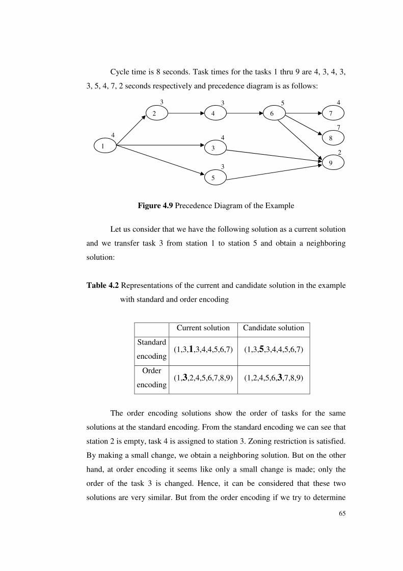
65
Cycle time is 8 seconds. Task times for the tasks 1 thru 9 are 4, 3, 4, 3,
3, 5, 4, 7, 2 seconds respectively and precedence diagram is as follows:
Figure 4.9 Precedence Diagram of the Example
Let us consider that we have the following solution as a current solution
and we transfer task 3 from station 1 to station 5 and obtain a neighboring
solution:
Table 4.2 Representations of the current and candidate solution in the example
with standard and order encoding
Current solution Candidate solution
Standard
encoding (1,3,1,3,4,4,5,6,7) (1,3,5,3,4,4,5,6,7)
Order
encoding (1,3,2,4,5,6,7,8,9) (1,2,4,5,6,3,7,8,9)
The order encoding solutions show the order of tasks for the same
solutions at the standard encoding. From the standard encoding we can see that
station 2 is empty, task 4 is assigned to station 3. Zoning restriction is satisfied.
By making a small change, we obtain a neighboring solution. But on the other
hand, at order encoding it seems like only a small change is made; only the
order of the task 3 is changed. Hence, it can be considered that these two
solutions are very similar. But from the order encoding if we try to determine
1
9
7
3
2 4
5
6
8
3
4
4
4
3
3 5
7
2
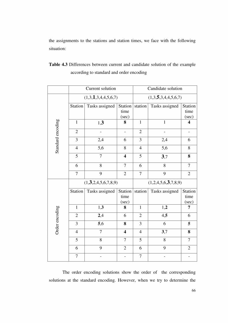
66
the assignments to the stations and station times, we face with the following
situation:
Table 4.3 Differences between current and candidate solution of the example
according to standard and order encoding
Current solution Candidate solution
(1,3,1,3,4,4,5,6,7) (1,3,5,3,4,4,5,6,7)
Station Tasks assigned Station
time
(sec)
station Tasks assigned Station
time
(sec)
1 1,3 8 1 1 4
2 - - 2 - -
3 2,4 6 3 2,4 6
4 5,6 8 4 5,6 8
5 7 4 5 3,7 8
6 8 7 6 8 7
Sta
ndar
d e
nco
din
g
7 9 2 7 9 2
(1,3,2,4,5,6,7,8,9) (1,2,4,5,6,3,7,8,9)
Station Tasks assigned Station
time
(sec)
station Tasks assigned Station
time
(sec)
1 1,3 8 1 1,2 7
2 2,4 6 2 4,5 6
3 5,6 8 3 6 5
4 7 4 4 3,7 8
5 8 7 5 8 7
6 9 2 6 9 2
Ord
er e
nco
din
g
7 - - 7 - -
The order encoding solutions show the order of the corresponding
solutions at the standard encoding. However, when we try to determine the
67
station numbers that tasks are assigned to and the station times, we face with
some difficulties. The first one is about the station numbers. We can not
understand the assignments from the order of tasks easily. If we try to compute
these numbers as explained in the paragraph of order encoding, we can obtain
any solution that does not represent the real situation as shown in the table. If
we try to fix the number of station as 3 that task 4 is assigned to, we can not be
sure that whether the task 2 is assigned to station 2 or station 3. The other
difficulty is about generating the neighboring solutions. It seems that only the
order of task 3 is changed. But if we try to determine the assignments and the
station times and calculate the objective value of this candidate solution (a
function of number of stations, cycle time, common tasks, batch sizes, etc.),
wee see that this new solution is very far from the current solution (The
changes about the solutions are bold-typed in Table 4.3). In conclusion, order
encoding may have an adverse effect on detailed search in a region. Because of
these disadvantages of order encoding, standard encoding is used in the
constructed algorithm.
4.8.2 The Move Procedure
Shift is used as the move procedure. A swap makes two shifts
simultaneously. Because swap mechanism is more restrictive than shift and
shift mechanism is more appropriate for making smaller changes on the current
solution, it is adopted as the move procedure.
Each of the two ASA algorithms designed in the study chooses a task k
randomly. Then the algorithm determines the set of stations that task k may be
assigned to by considering precedence relationships, cycle time, station times
and zoning restrictions. Then the task k is moved to a station which is chosen
randomly from this set.
68
4.8.3 The Adaptive Cooling Schedule
The Simulated Annealing approach can not escape from a local optima
if acceptance probability is very small. As it is mentioned in the previous
sections, the main idea of Adaptive Simulated Annealing is adjusting the
algorithm according to the past search. In order to escape from local optimums,
logic of the approach allows reheating. If so, the main job is to develop such a
method that the algorithm perceives that it is in a local optimal region and it is
difficult to escape from there. There are two dimensions about the subject. The
first one is being in a local optimal region and the second one is being unable
to escape from there. The SA algorithm generates a neighboring solution and if
it is a better solution, the algorithm passes to that solution; if it is an inferior
solution, the algorithm passes to that solution according to the acceptance
probability. If the number of inferior solutions in the recently generated
neighboring solutions increases, it may be a sign to being in a local optimal
region. If the number of inferior solutions in the recently generated neighboring
solutions is very high, it may be a sign to being in a local optimal region and
not passing to inferior solutions. If the algorithm generates and passes to an
inferior solution, then the probability to generate a better solution increases and
the number of inferior solutions decreases. On the other hand, the algorithm
may be in a local optimal region, but if the acceptance probability is
sufficiently high, it may escape from that region. But if the ratio of accepted
inferior solutions in the whole inferior solutions in the recently generated
solutions is very low, it may be a sign to understand that the temperature is not
high enough to escape from that region.
The cooling schedule used in the algorithm is given below:
Tem[i]=K / j
where Tem[i] is the temperature at iteration i, j is a counter that controls
the temperature and K is a positive integer.
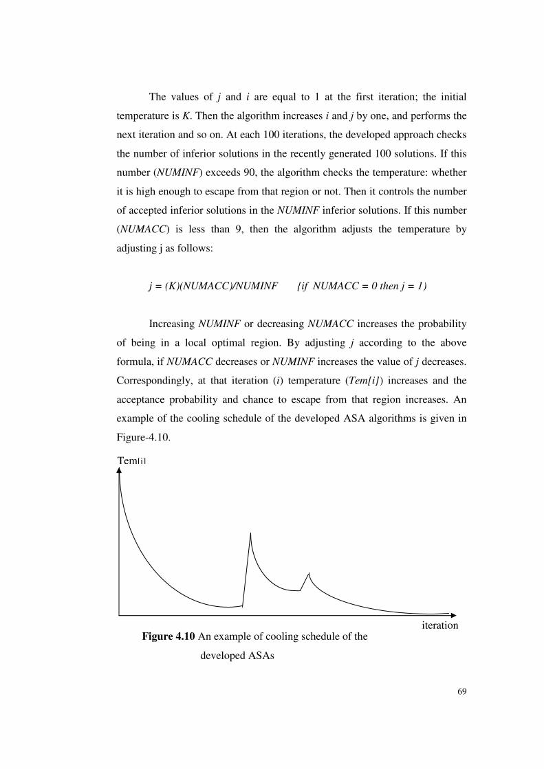
69
The values of j and i are equal to 1 at the first iteration; the initial
temperature is K. Then the algorithm increases i and j by one, and performs the
next iteration and so on. At each 100 iterations, the developed approach checks
the number of inferior solutions in the recently generated 100 solutions. If this
number (NUMINF) exceeds 90, the algorithm checks the temperature: whether
it is high enough to escape from that region or not. Then it controls the number
of accepted inferior solutions in the NUMINF inferior solutions. If this number
(NUMACC) is less than 9, then the algorithm adjusts the temperature by
adjusting j as follows:
j = (K)(NUMACC)/NUMINF {if NUMACC = 0 then j = 1)
Increasing NUMINF or decreasing NUMACC increases the probability
of being in a local optimal region. By adjusting j according to the above
formula, if NUMACC decreases or NUMINF increases the value of j decreases.
Correspondingly, at that iteration (i) temperature (Tem[i]) increases and the
acceptance probability and chance to escape from that region increases. An
example of the cooling schedule of the developed ASA algorithms is given in
Figure-4.10.
iteration
Tem[i]
Figure 4.10 An example of cooling schedule of the
developed ASAs
70
4.8.4 Construction of the Initial Solution
In real life, assembly lines generally include some zoning restrictions.
Because of the zoning restrictions, while constructing a solution, we have to
consider the list of stations that any task may be assigned to. As a result, at any
iteration in the construction algorithm, we can not use only available tasks; we
have to use the assignable tasks to the current station. Therefore, we have
constructed a station-oriented and modified COMSOAL algorithm to generate
a feasible starting solution. The algorithm first determines the available tasks
from the precedence diagram. Then it chooses the assignable tasks among the
available tasks by checking the zoning restrictions, the cycle time and the
station time. After that, the algorithm takes a task randomly among the
assignable tasks and assigns it to the current station. Then it updates the
available and assignable tasks by considering the last assignment. If there is no
assignable task, it passes to the next station. Because of the zoning restrictions,
occasionally, there may be no assignable task, although the station is opened
recently and empty. The modification on COMSOAL is about the zoning
restrictions.
4.8.5 Evaluating the Solutions
4.8.5.1 Evaluating the Line Balances
Upon completing the COMSOAL routines, the algorithm passes to the
ASA phases to improve the solution. Because the problem may be multi/mixed
or single-model assembly line balancing problem and it is multi-objective, it
requires using two ASA parts sequentially.
As it is mentioned in Chapter 2, there are two main approaches to
balance the multi-model assembly lines. The first one is balancing the line

71
separately for each model as a single-model assembly line balancing, while the
second one is balancing the line as if it is a mixed-model assembly line.
When the first approach is accepted, the system uses the minimum
number of stations for each model and avoids the costs related to the unused
station at the period of that model’s production. But, in this situation, the
number of the common tasks assigned to different stations and the changes on
the set of tasks assigned to the same station increase. Consequently, the setup
costs and negative learning curve effect increase. When the batch sizes are very
large, the advantages of this method dominate its disadvantages and, in general,
this approach is adopted.
When the second approach is accepted, the problem is considered as a
mixed-model assembly line balancing, and generally, by using the combined
precedence diagram, a single balance is found for all models. With this
approach, all common tasks are assigned to the same stations. When the
production changes over to a new model, some tasks are extracted from the line
and some others are added to the line. Hence, there still exists additional setup
cost and learning curve effect, but it is minimized. Nevertheless, this time, the
number of stations and the station slack times increase for each model.
Furthermore, opportunity to increase smoothness and to minimize cycle time
and their advantages can not be utilized. When the batch sizes are very small,
the second approach is adopted, since the advantages of this approach generally
dominate its disadvantages.
The first method assumes that the setup costs and the learning curve
effects are negligible compared to the gain from balancing separately. On the
other hand, the second method assumes that its disadvantages are negligible
compared to its advantages. If the batch sizes are medium and none of the costs
is negligible, balancing the line gets harder. In this situation, there exists
challenging objectives. One of them is minimizing the number of stations while

72
trying to maximize the common tasks assigned to the same station. The other
one is minimizing the cycle time, while trying to maximize the common tasks
assigned to the same station. Although it is possible to decrease the number of
stations or the cycle time and to increase smoothness, common tasks may
prevent the method from making these moves.
As it is mentioned in the previous parts, in order to minimize the cycle
time or maximize smoothness, the number of stations and a feasible solution
must be pre-determined. In addition, maximization of irregularity and
maximization of smoothness are exactly opposites. So, they should be used
separately. For these reasons, the proposed algorithm first tries to minimize the
number of stations and uses maximization of irregularity while considering the
common tasks and batch sizes. Then, it uses this solution as an input to the next
ASA part and tries to minimize the cycle time and the total slack time, while
maximizing the smoothness. The algorithm, at this stage, also takes the
common tasks and batch sizes into account.
The objective functions used to evaluate the solutions in the first ASA
(Ffirst[x]) and in the second ASA (Fsecond[x]) are given below:
Ffirst[x] = F1[x] + F3[x] + F5[x]
Fsecond[x] = F2[x] + F4[x] + F5[x]
where x is a line balance and,
F1[x] is the objective function used to minimize number of stations,
F2[x] is the objective function used to minimize cycle time,
F3[x] is the objective function used to maximize irregularity,
F4[x] is the objective function used to maximize smoothness,
F5[x] is the objective function used to maximize common tasks
assigned to same station.
73
Because of the structure of the SA algorithm, the solutions are
evaluated separately at the sequential ASA algorithms. But the whole problem
is balancing the line and determining the best sequence. For single-model lines
because the number of product models is one the sequencing problem drops.
Similar to the single-model lines, because of the combined precedence diagram
for mixed-model lines, the sequencing problem again drops. The best solution
found for a model i is evaluated with the objective function of balancing model
i ( Fmodeli[x] ) which is given below:
Fmodeli[x]=F2[x]+F4[x]+F5[x]
Here, F2[x] evaluates the solution according to the cycle time, number
of used stations and batch sizes; F4[x] evaluates the solution according to the
smoothness; F5[x] evaluates it according to the common tasks between the
current model (i) and the previous model. Because F1[x] is identical with
F2[x] and maximization of irregularity (F3[x]) is not really a desired objective,
these two components are not used to evaluate the final balance of model i.
4.8.5.2 Evaluating the Sequences
The other problem is the sequencing problem. In order to evaluate the
whole solution which consists of both the individual model balances and the
sequence of these models, it is needed to use a more widespread objective
function: F[x] which is given below:
For a single-model i (or mixed-model) line balancing, F[x] transforms
to Fmodeli[x] (or Fmodelcombined[x] ).
zerohan greather t is sizebatch which of models ofset theis where K
[x]FmodelF[x]Ki
i∑∈∀
=

74
4.8.6 The Overall Methodology
The explained methodology is used to balance any type of assembly
line. This methodology, consisting of the modified COMSOAL and two ASA
algorithms to solve the multi-objective assembly line balancing problems, used
as a main block and as an inner part of the complete algorithm. The external
part of the algorithm adjusts the usage of the inner part. The external part
determines the type of the assembly line, batch sizes of the models and the
period of the production. If the assembly line is a single-model assembly line
or the user wants to balance the line for a single-model, the external part
computes the cycle time and runs the main part for this single-model only.
Because of the minimization of the cycle time in the second ASA, the
algorithm saves some time and the external part computes this time and reports
it along with the assignments.
If the line is mixed-model assembly line, the algorithm uses the
combined precedence diagram and finds a single common solution for all
models.
If the line is multi-model assembly line, the external part first gets the
batch sizes and the production period. Then it determines the first sequence of
the models and runs the inner part for the first model in the sequence. The
external part then computes the remaining time, calculates the cycle time and
runs the inner part again for the next model in the sequence. After completing
all models, the external part determines the next sequence and runs the inner
part for all models once more. At the end, the algorithm finds the best sequence
and all individual assignments.
If the line consists of some models with large batch sizes and some
others with small batch sizes, the user may easily set the cost parameters and
find a good solution suitable for this situation. If the line includes only the
models with large batch sizes or small batch sizes, the user may balance the
75
line as a single-model assembly line for all models with large batch sizes or as
a mixed-model assembly line or he/she may adjust the cost parameters and find
solutions between these two extremes. Furthermore, the firm may select some
of the models to produce and the algorithm finds the best sequence and the
individual assignments for only those selected models. Figure 4.11 shows the
flowchart of the methodology and the pseudocode of the whole algorithm is
given in Appendix D.

76
Figure 4.11 Flowchart of the algorithm
N
N
Pass next model in the
sequence
Pass another untried
sequence
For the current sequence is it
completed to balance the line for all
models?
Is it completed to balance the line for
all possiblesequences?
STOP
Y
Y
Record the best sequence and
balances of models
Compute the remaining time and cycle
time
For the model construct a feasible
initial solution by using COMSOAL
First ASA part to minimize number of
stations and maximize common tasks
Second ASA part to minimize cycle
time and maximize common tasks
Get the type of the assembly line
Get the batch size(s)
Get the production period
Get the precedence relationships, task
times and zoning restrictions
Determine the sequence(s) of the
model(s)

77
CHAPTER 5
EXPERIMENTAL ANALYSIS
5.1 Design of the Experiment
The proposed algorithm may be used to solve single, mixed or multi-
model assembly line balancing problems. Furthermore, a problem may be
solved by taking one or more objectives into account. Because the structure of
the algorithm changes under different objective combination and assembly line
type scenarios, the performance of the algorithm should be evaluated according
to these scenarios.
There are five objective function components in the algorithm, but these
objectives may be grouped in three classes. The first one is minimization of the
number of used stations. Because the maximization of irregularity is sub
objective to achieve minimization of the number of used stations and they are
not conflicting objectives with each other, these two components may be
considered as the first objective group. Similarly, the maximization of
smoothness is sub objective to achieve minimization of cycle time and these
two components may be considered as the second objective group. On the
other hand, the maximization of common tasks which are assigned to the same
station at the assembly of successive models is another objective class by itself.
These three objectives are conflicting objectives with each other. One of the
methods to deal with conflicting objectives is to take them into account
successively. In this method, the problem is solved according to the first
objective, then it is solved according to the next objective such that the
previous solution is satisfied. Another method to deal with conflicting

78
objectives is to give these objectives weights and to solve the problem
according to these objectives simultaneously. The developed algorithm uses
these two methods to overcome the difficulty of conflicting objectives. The
first two objective groups are separated by using two ASA algorithms. The first
ASA part tries to find the best solution according to the first and the third
objective groups. On the other hand the second ASA part tries to find the best
solution according to the second and the third objective groups such that the
previous solution found in the first ASA part is satisfied.
The proposed algorithm solves the mixed-model assembly line
balancing problems by using the combined precedence diagram method. This
method transforms the problem to a single-model assembly line balancing
problem. The third objective group is redundant when the problem is single-
model or mixed-model assembly line balancing problem. Because the other
two objective groups are used separately, for the single-model and mixed-
model assembly line balancing problems, the performance of the first ASA part
may be evaluated according to the minimization of the number of used stations
and the performance of the second ASA part may be evaluated according to the
minimization of cycle time. For this purpose, the test problems of SALBP-I
from the literature are used to evaluate the performance of the first ASA part
and those of SALBP-II are used to evaluate the performance of the second
ASA part. Then the algorithm is tested on the case problem and it is run 10
times, and the results are analyzed. For the single and mixed-model assembly
line balancing problems, the experimental analysis is explained in the
following sections. The analysis about the multi-model assembly line balancing
problems is explained in the following sections.
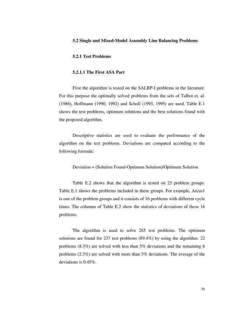
79
5.2 Single and Mixed-Model Assembly Line Balancing Problems
5.2.1 Test Problems
5.2.1.1 The First ASA Part
First the algorithm is tested on the SALBP-I problems in the literature.
For this purpose the optimally solved problems from the sets of Talbot et. al.
(1986), Hoffmann (1990, 1992) and Scholl (1993, 1995) are used. Table E.1
shows the test problems, optimum solutions and the best solutions found with
the proposed algorithm.
Descriptive statistics are used to evaluate the performance of the
algorithm on the test problems. Deviations are computed according to the
following formula:
Deviation = (Solution Found-Optimum Solution)/Optimum Solution
Table E.2 shows that the algorithm is tested on 25 problem groups.
Table E.1 shows the problems included in these groups. For example, Arcus1
is one of the problem groups and it consists of 16 problems with different cycle
times. The columns of Table E.2 show the statistics of deviations of these 16
problems.
The algorithm is used to solve 265 test problems. The optimum
solutions are found for 237 test problems (89.4%) by using the algorithm. 22
problems (8.3%) are solved with less than 5% deviations and the remaining 6
problems (2.3%) are solved with more than 5% deviations. The average of the
deviations is 0.45%.
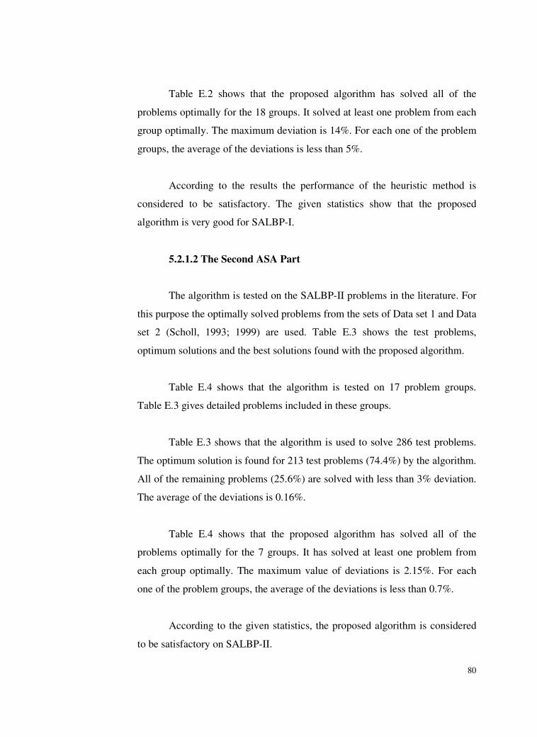
80
Table E.2 shows that the proposed algorithm has solved all of the
problems optimally for the 18 groups. It solved at least one problem from each
group optimally. The maximum deviation is 14%. For each one of the problem
groups, the average of the deviations is less than 5%.
According to the results the performance of the heuristic method is
considered to be satisfactory. The given statistics show that the proposed
algorithm is very good for SALBP-I.
5.2.1.2 The Second ASA Part
The algorithm is tested on the SALBP-II problems in the literature. For
this purpose the optimally solved problems from the sets of Data set 1 and Data
set 2 (Scholl, 1993; 1999) are used. Table E.3 shows the test problems,
optimum solutions and the best solutions found with the proposed algorithm.
Table E.4 shows that the algorithm is tested on 17 problem groups.
Table E.3 gives detailed problems included in these groups.
Table E.3 shows that the algorithm is used to solve 286 test problems.
The optimum solution is found for 213 test problems (74.4%) by the algorithm.
All of the remaining problems (25.6%) are solved with less than 3% deviation.
The average of the deviations is 0.16%.
Table E.4 shows that the proposed algorithm has solved all of the
problems optimally for the 7 groups. It has solved at least one problem from
each group optimally. The maximum value of deviations is 2.15%. For each
one of the problem groups, the average of the deviations is less than 0.7%.
According to the given statistics, the proposed algorithm is considered
to be satisfactory on SALBP-II.
81
The experiments on the test problems showed us that the performance
of the first ASA part is very good at the minimization of the number of used
stations and the performance of the second ASA part is very good at the
minimization of cycle time, when the third objective group which is conflicting
with the first two objective groups is neglected. The performance of the
algorithm is very good at single-model assembly line balancing problems.
Furthermore, because we transform the mixed-model problems to single-model
problems by using combined precedence diagram method, the performance of
the algorithm is also very good at mixed-model assembly line balancing
problems at our case study. After these experiments the algorithm is tested on
the case problem.
5.2.2 The Case Problem
Two factors are defined for these experiments: model and batch size.
Levels of the model are Model1, Model2, Model3, Model4 and Mixed. Levels
of the production amounts are 300, 500 and 600 units per shift; during the
production period a single model, or more then one model with mixed-model
type, is produced with batch size 300, 500 and 600 units. Then the response
variables are used to analyze the effects of the factors on the performance of
the algorithm. Response variables are the number of used stations (m), cycle
time (C), total slack time (TST) and deviations from the theoretical optimums
of the number of stations (Dm) and cycle time (DC) at the beginning of the run
and at the end of the run. Table 5.1 shows the average and standard deviation
values of the response variables for 10 runs.
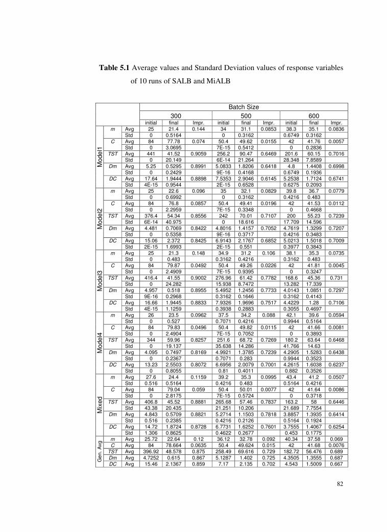
82
Table 5.1 Average values and Standard Deviation values of response variables
of 10 runs of SALB and MiALB
Batch Size
300 500 600 initial final Impr. initial final Impr. initial final Impr.
Avg 25 21.4 0.144 34 31.1 0.0853 38.3 35.1 0.0836 m
Std 0 0.5164 0 0.3162 0.6749 0.3162
Avg 84 77.78 0.074 50.4 49.62 0.0155 42 41.76 0.0057 C
Std 0 3.0695 7E-15 0.5412 0 0.2836 Avg 441 41.52 0.9059 256.2 90.47 0.6469 201.6 60.15 0.7016 TST
Std 0 20.149 6E-14 21.264 28.348 7.8589
Avg 5.25 0.5295 0.8991 5.0833 1.8206 0.6418 4.8 1.4408 0.6998 Dm
Std 0 0.2429 9E-16 0.4168 0.6749 0.1936
Avg 17.64 1.9444 0.8898 7.5353 2.9046 0.6145 5.2538 1.7124 0.6741
Mode
l1
DC
Std 4E-15 0.9544 2E-15 0.6528 0.6275 0.2093
Avg 25 22.6 0.096 35 32.1 0.0829 39.8 36.7 0.0779 m
Std 0 0.6992 0 0.3162 0.4216 0.483
Avg 84 76.8 0.0857 50.4 49.41 0.0196 42 41.53 0.0112 C
Std 0 2.2959 7E-15 0.3348 0 0.4668
Avg 376.4 54.34 0.8556 242 70.01 0.7107 200 55.23 0.7239 TST
Std 6E-14 40.975 0 18.616 17.709 14.596
Avg 4.481 0.7069 0.8422 4.8016 1.4157 0.7052 4.7619 1.3299 0.7207 Dm
Std 0 0.5358 9E-16 0.3717 0.4216 0.3483
Avg 15.06 2.372 0.8425 6.9143 2.1767 0.6852 5.0213 1.5018 0.7009
Mo
de
l2
DC
Std 2E-15 1.6993 2E-15 0.551 0.3977 0.3843
Avg 25 21.3 0.148 34.9 31.2 0.106 38.1 35.3 0.0735 m
Std 0 0.483 0.3162 0.4216 0.3162 0.483
Avg 84 79.87 0.0492 50.4 49.26 0.0226 42 41.81 0.0045 C
Std 0 2.4909 7E-15 0.9395 0 0.3247
Avg 416.4 41.55 0.9002 276.96 61.42 0.7782 168.6 45.36 0.731 TST
Std 0 24.282 15.938 8.7472 13.282 17.339
Avg 4.957 0.518 0.8955 5.4952 1.2456 0.7733 4.0143 1.0851 0.7297 Dm
Std 9E-16 0.2968 0.3162 0.1646 0.3162 0.4143
Avg 16.66 1.9445 0.8833 7.9326 1.9696 0.7517 4.4229 1.28 0.7106
Mode
l3
DC
Std 4E-15 1.1259 0.3938 0.2883 0.3055 0.4697
Avg 26 23.5 0.0962 37.5 34.2 0.088 42.1 39.6 0.0594 m
Std 0 0.527 0.7071 0.4216 0.9944 0.5164 Avg 84 79.83 0.0496 50.4 49.82 0.0115 42 41.66 0.0081 C
Std 0 2.4904 7E-15 0.7052 0 0.3893
Avg 344 59.96 0.8257 251.6 68.72 0.7269 180.2 63.64 0.6468 TST
Std 0 19.137 35.638 14.286 41.766 14.63
Avg 4.095 0.7497 0.8169 4.9921 1.3785 0.7239 4.2905 1.5283 0.6438 Dm
Std 0 0.2367 0.7071 0.283 0.9944 0.3523 Avg 13.23 2.5503 0.8072 6.6956 2.0079 0.7001 4.2615 1.6038 0.6237
Mo
de
l4
DC
Std 0 0.8055 0.81 0.4011 0.882 0.3526
Avg 27.6 24.4 0.1159 39.2 35.3 0.0995 43.4 41.2 0.0507 m
Std 0.516 0.5164 0.4216 0.483 0.5164 0.4216
Avg 84 79.04 0.059 50.4 50.01 0.0077 42 41.64 0.0086 C
Std 0 2.8175 7E-15 0.5724 0 0.3718 Avg 406.8 45.52 0.8881 265.68 57.46 0.7837 163.2 58 0.6446 TST
Std 43.38 20.435 21.251 10.206 21.689 7.7554
Avg 4.843 0.5709 0.8821 5.2714 1.1503 0.7818 3.8857 1.3935 0.6414 Dm
Std 0.516 0.2385 0.4216 0.2126 0.5164 0.1924
Avg 14.72 1.8724 0.8728 6.7731 1.6252 0.7601 3.7555 1.4067 0.6254
Mix
ed
DC
Std 1.306 0.8625 0.4622 0.2677 0.453 0.1775
m Avg 25.72 22.64 0.12 36.12 32.78 0.092 40.34 37.58 0.069
C Avg 84 78.664 0.0635 50.4 49.624 0.015 42 41.68 0.0076
TST Avg 396.92 48.578 0.875 258.49 69.616 0.729 182.72 56.476 0.689
Dm Avg 4.7252 0.615 0.867 5.1287 1.402 0.725 4.3505 1.3555 0.687
Gen.
Avg
DC Avg 15.46 2.1367 0.859 7.17 2.135 0.702 4.543 1.5009 0.667
83
The cycle time is computed as the production period (7 hours=a shift)
divided by the total production amount. If the batch size increases, the initial
value of cycle time decreases. If batch size is 300, 500 or 600 units, the
corresponding initial values of cycle time are 84, 50.4 or 42 seconds.
Improvement values are computed for a response variable as follows:
Improvement = (initial value-final value)/initial value
For each model, but Model1, improvement in number of stations (m)
decreases, when batch size increases or initial value of cycle time decreases.
General averages show that the improvement in m decreases, when batch size
increases. It means that the performance of the first ASA part increases, when
the initial cycle time increases.
For each model, but Mixed, improvement in C decreases, when batch
size increases. If the batch size increases, the initial cycle time decreases and
the number of stations needed increases. The general average values of m are
22.64, 32.78 and 37.58. When the number of stations increases, it is expected
that the final value of cycle time would be lower and the improvement in the
cycle time would increase. But results show the opposite of it; the
improvement in C decreases when the number of stations increases.
For Model3, Model4 and Mixed, the improvement in TST decreases
when batch size increases. For Model1 and Model2, the improvement in TST
fluctuates, but in general, it decreases when the initial cycle time decreases.
Because the improvement in m and C decreases, the result about TST is
expected.
The results summarized above show that improvement in m, C and TST
decreases, when the initial cycle time decreases, or equivalently, when the
84
amount of production per shift increases. Consequently, as the initial cycle
time increases, the performance of the algorithm gets better.
Deviation from the lower bound of the number of stations (Dm) is
computed as:
Dm = (TST)/C
The integer part of Dm shows the maximum number by which the
number of stations may be decreased to reach the theoretical minimum at that
cycle time. The interesting result is that the integer part of Dm value with 300
batch size is zero for each model. It shows that the algorithm finds the
optimum solutions. This value increases to 1 with 500 and 600 batch sizes. It
means that the solution found deviates from the lower bound by one station
only. In general, the improvement in Dm decreases, when the batch size
increases.
Deviation from the lower bound of cycle time (DC) is computed
according to the following formula:
DC = (TST)/m
If cycle time may be decreased by DC units, the perfect balance is
obtained. The results show that DC value fluctuates with the batch size for
individual models, but in general averages it decreases, when the batch size
increases. Improvement in DC decreases when the initial cycle time decreases.
At the end of the runs deviations from the lower bound of cycle time do not
exceed 2 seconds.
For each model but Mixed, at the end of the run, the standard deviation
of m is the smallest at 500 units per shift. The biggest value of standard
85
deviations of m is 0.699 stations. For each model but Model1, at the end of the
run, the standard deviation of C decreases, when the batch size increases. The
biggest value of standard deviations of C is 3.069 seconds. For 500 units of
production, this value decreases to 0.9 seconds. Standard deviation of TST
fluctuates with batch sizes and models. Also the standard deviation of Dm
fluctuates with batch sizes and models. For each model, standard deviation of
DC decreases, when the batch size increases.
The most important results are about Dm and DC values, because these
values give an opinion about the quality of the solutions. The deviations from
the lower bound do not exceed 3% for the number of stations and 4% for the
cycle time. Standard deviations of Dm do not exceed 0.53 stations and standard
deviations of DC do not exceed 1.699 seconds. According to the results the
algorithm finds very good solutions for the case problem, because the
deviations from the lower bounds are less than 5%. Since the current amount of
production per shift is 500, the convergence graphics with 500 batch size are
given in Appendix E.
5.3 Multi-Model Assembly Line Balancing Problems
When the problem is multi-model assembly line balancing problem, the
third objective group is to be taken into account which conflicts with the first
two objectives. If the weight of the third objective is negligible, the
assignments of the common tasks to the different stations get free, transforming
the problem to a SALBP for each model. The performance of the algorithm is
examined in the previous sections. On the other hand, if the weight of the third
objective group is very high, it forces the algorithm to assign all of the
common tasks to the same stations. In this situation, the problem shifts to a
MiALBP which makes assignments by using the combined precedence
diagram and obtains a single balance for all models. The performance of the
algorithm is also studied in the previous sections in this situation. For
86
MuALBP, the problem has to be solved as a MuALBP. The test problems for
MuALBP which consist of conflicting objectives could not be obtained from
the literature. The analysis is made on the case problem. The problem is solved
with three different weights of the third objective. For each one of the weights,
the algorithm is run 10 times and the results are evaluated. The percentages of
the number of common tasks which are assigned to the same stations and the
effects of the third objective to the other objectives are analyzed.
The weights of the third objective group are low, intermediate and high.
The daily batch sizes of the Model1, Model2, Model3 and Model4 are 350, 75,
50 and 25 units, respectively. At low level of the weight of the third objective,
the contribution of the third objective is similar to the contributions of the other
objectives for Model4. At intermediate level of the weight of the third
objective, the contribution of the third objective is similar to the contributions
of the other objectives for Model2 and it is similar to the contributions of the
other objectives for Model1 at the high level of the weight of the third
objective.
Table E.5 shows the sequences of the models and number of common
tasks between models. Tables E.6, E.7 and E.8 show the numbers of common
tasks that are assigned to the same stations at the successive models and their
percentages. The values are average of 10 runs for each level of the third
objective. For low, intermediate and high level of the weight of the third
objective, the overall averages of percentages are 47.88%, 88.54% and 94%,
respectively. These results indicate that the algorithm is sensitive to the third
objective. The results show that when the weight of the third objective is at
intermediate or higher levels, the algorithm assigns approximately 90% of the
common tasks to the same stations.
Total slack time, number of used stations and cycle time values are
recorded throughout the runs. Table 5.2 shows the average values of number
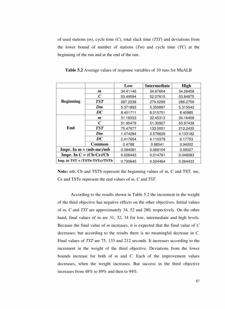
87
of used stations (m), cycle time (C), total slack time (TST) and deviations from
the lower bound of number of stations (Tm) and cycle time (TC) at the
beginning of the run and at the end of the run.
Table 5.2 Average values of response variables of 10 runs for MuALB
Low Intermediate High
m 34.41146 34.87604 34.26458
C 53.49594 52.07615 53.84875
TST 287.2238 279.0299 286.2759
Dm 5.371893 5.350897 5.315542
Beginning
DC 8.401711 8.015751 8.40985
m 31.18333 32.45313 34.16458
C 51.95479 51.30927 50.97438
TST 75.47677 133.0051 212.2435
Dm 1.474284 2.578629 4.133182
DC 2.417654 4.110379 6.17753
End
Common 0.4788 0.88541 0.94002
Impr. In m = (mb-me)/mb 0.094081 0.069104 0.00027
Impr. In C = (Cb-Ce)/Cb 0.028443 0.014781 0.049083
Imp. in TST = (TSTb-TSTe)/TSTb 0.730645 0.524464 0.264433
Note: mb, Cb and TSTb represent the beginning values of m, C and TST. me,
Ce and TSTe represent the end values of m, C and TST.
According to the results shown in Table 5.2 the increment in the weight
of the third objective has negative effects on the other objectives. Initial values
of m, C and TST are approximately 34, 52 and 280, respectively. On the other
hand, final values of m are 31, 32, 34 for low, intermediate and high levels.
Because the final value of m increases, it is expected that the final value of C
decreases; but according to the results there is no meaningful decrease in C.
Final values of TST are 75, 133 and 212 seconds. It increases according to the
increment in the weight of the third objective. Deviations from the lower
bounds increase for both of m and C. Each of the improvement values
decreases, when the weight increases. But success in the third objective
increases from 48% to 89% and then to 94%.
88
Tables from E.9 to E.32 in the Appendix E show the detailed results
about the first, second, third and the last model in a sequence; Model1,
Model2, Model3 and Model4; m, C and TST. General results obtained from
these detailed results are summarized in Table 5.2 above.
5.4 Current Line Balance and Suggested Line Balances
According to the current balance, for Model1, Model2 and Model3 the
number of used stations is 36, while it is 37 for Model4. When the line passes
to produce Model4, station numbers of nine tasks change. As it is mentioned in
Chapter3, the system finds this solution in a week, but the suggested method
uses computers and balances the line in some minutes for the mixed-model
case and in a few hours for multi-model case. Daily productions of Model1,
Model2, Model3 and Model4 are taken as 350, 75, 50 and 25 units,
respectively. On the other hand, in this study, the balancing problem of the
company is solved according to the multi-model case. According to the
suggested solution, numbers of the used stations for Model1, Model2, Model3
and Model4 are 31, 30, 30 and 31, respectively. Daily production amounts are
the same. Production sequence is Model1, Model3, Model2, Model4. Stations
of 43, 22 and 18 tasks change, when the system passes from Model1 to
Model3, from Model3 to Model2 and from Model2 to Model4, respectively. If
the system prefers to balance the line as a mixed-model line, the proposed
method finds a solution with the number of used stations as 35, and all of the
common tasks being assigned to the same stations. The current assignments
and the suggested assignments are given in Appendix F.
5.5 Run Times of the Experiments
The algorithm is coded in Turbo Pascal Windows and the runs are made
in a computer specifications of which are Intel Pentium 4, CPU 3 GHz, 512
MB RAM.

89
The algorithm is run for 10 minutes for each of the test problems and
the best solutions are recorded.
For the experimental runs about the case problem, the algorithm is run
for a limited number of iterations; 10000 iterations for each ASA part. The
computer completes a run for any model in about 1-1.5 minutes. i.e., the
algorithm finishes the run in 1-1.5 minutes for single-model or mixed-model
balancing cases. For the multi-model case, the algorithm solves an individual
single-model balancing for all sequences and for each of the models in a
sequence. Because the case consists of 4 models, the algorithm makes 96
(4*4!) individual balancing and the whole run is completed in approximately
96-144 minutes.

90
CHAPTER 6
CONCLUSION AND FURTHER RESEARCH ISSUES
In this study, we deal with a real-life assembly line balancing problem
and propose an approach which solves each type of SALBP, MiALBP and
MuALBP with zoning restrictions. The proposed algorithm solves multi-
objective assembly line balancing problems as well. Because the proposed
algorithm has a flexible structure, it may be used to solve each type of
assembly line balancing problems, furthermore, it is also appropriate to solve
harder problems, real-life problems because it considers different objectives
and zoning restrictions.
When the problem includes more than one and conflicting objectives, it
gets harder to solve the problem. Assembly line balancing problems, especially
multi/mixed model assembly line balancing problems, are complex problems,
and generally consist of more than one conflicting objectives. Number of used
stations, cycle time, common tasks among models, setup cost of passing from
production of a model to another one’s, etc. are some of the factors that affect
the solution of the assembly line balancing problems.
Especially for the multi model assembly lines, sequencing arises as
another problem besides the line balancing problem. Because the common
tasks between sequential models change with respect to the models, it becomes
important to determine the best sequence. If so, without balancing the line for
each model, determining the true sequence of the models becomes another
problem.

91
Most of the real-life problems are complex ones and consist of zoning
restrictions, multi-model or mixed-model situations, conflicting objectives etc.
which make the problem even harder. Although the real-life problems consist
of these complexities most of the studies in the literature are about SALBPs. In
this study, we attempt to solve a real-life multi-objective multi-model assembly
line balancing problem with many zoning restrictions for which there is as yet
no optimum-seeking algorithm in the literature. Because of these complexities
of the problem, we have constructed a flexible heuristic algorithm and used to
solve it. The developed approach is proposed to solve such complex assembly
line balancing problems.
The developed algorithm uses a modified COMSOAL algorithm to
construct an initial solution and two sequential ASA algorithms to improve the
solution. To solve MuALBPs, the algorithm uses five objective function
components to evaluate the solutions, regarding the three conflicting
objectives. The first ASA algorithm tries to minimize the number of stations
while trying to maximize the number of common tasks which are assigned to
the same stations. The second ASA algorithm tries to minimize the cycle time
while trying to maximize the number of common tasks assigned to the same
stations by considering the batch sizes as well as the first ASA algorithm’s
results. Then the algorithm passes to the next models and next sequences. At
the end of the run, the algorithm finds individual balances for each model and
the best sequence of the models. To solve MiALBPs, the algorithm uses the
combined precedence diagram method. Because the algorithm finds a single
balance for all models, the sequencing problem and therefore the objective of
maximization of number of common tasks which are assigned to the same
stations at the sequential models drop. Thus as well as the SALBPs for the
MiALBPs the first ASA algorithm tries to minimize only the number of used
stations and the second ASA algorithm tries to minimize only the cycle time.

92
In this study, we have tested the proposed algorithm on test problems
from the literature and on the case problem as well. For each type of the
assembly line balancing problem, the experimental results are analyzed
separately. The results may be summarized as follows:
The algorithm is tested on 265 SALBP-I problems from the literature.
The optimum solution is found in 237 of the 265 test problems (89.4%) by the
algorithm. On the average, for any cycle time, the proposed algorithm solves
the problem with 0.45% deviation from the optimum solution. The given
statistics show that the proposed algorithm is very good on SALBP-I. The
algorithm is also tested to solve 286 SALBP-II test problems. The optimum
solution is found in 213 of the 286 test problems (74.4%) by the algorithm. The
proposed algorithm is very good on SALBP-II as well.
The algorithm is tested on the case problem for single-model and mixed
model cases. According to the results the algorithm finds very good solutions
for the case problem. The deviations from the lower bound does not exceed 3%
in the number of stations and 4% in the cycle time. The solution for the case
problem may be the optimum solution, but theoretically the number of stations
may be decreased by ‘1’, when the total amount of daily production increases.
On the other hand, if the total amount of daily production increases, i.e. the
initial cycle time decreases, the deviation from the theoretical minimum (lower
bound) of the cycle time decreases. The deviation from the lower bound does
not exceed 2 seconds (4%).
The algorithm is finally tested on the case problem for the multi-model
case. As it is expected, the increase in the weight of the ‘common tasks’
objective affects the other objectives adversely; if the weight is increased, the
deviations from the lower bounds increases up to 4 stations and 6.17 seconds.
But the percentage of the common tasks that are assigned to the same stations
increases to 94%.

93
At the end of this study, some worthwhile contributions to the company
can be stated as follows:
Task list has been updated and corrected. The tasks which are
performed on the line but are not defined yet are defined and coded. The tasks
which were formerly performed more than once on the line, but coded and
named once in the list, are defined and coded separately. Some automatically
made tasks are defined and added to the list.
The assembly line and the models of the product are observed;
precedence relationships diagram for each individual model and combined
precedence relationships diagram are constructed. Zoning restrictions are
determined.
A meta-heuristic approach is developed and computer program of the
method is coded. Thus, the disadvantages of balancing the line manually are
eradicated. It is possible to balance the line in some minutes for the mixed-
model case or in some hours for the multi-model case for the assembly line
under study.
According to the current balance in the plant, the number of stations is
36 for Model1, Model2 and Model3, and 37 for Model4. When the line passes
to produce Model4, station numbers of 9 tasks change. Daily productions of
Model1, Model2, Model3 and Model4 are 350, 75, 50 and 25 units,
respectively. On the other hand, in this study, the balancing problem of the
company is solved according to the multi-model case. According to our
suggested solution, numbers of stations for Model1, Model2, Model3 and
Model4 are 31, 30, 30 and 31, respectively. Daily production amounts are the
same. Production sequence is Model1, Model3, Model2, Model4. Station
numbers of 17, 32 and 16 tasks change when the system passes from Model1 to
Model3, from Model3 to Model2 and from Model2 to Model4. If the system
94
prefers to balance the line as a mixed-model line, the proposed method finds a
solution with 35 stations.
The contributions of this study to the literature may be summarized as
follows:
We offer to use an objective function that maximizes the irregularity
among station times (workloads) in order to minimize the number of used
stations. Similarly, we offer an objective function that maximizes the
smoothness in order to minimize the cycle time.
We use an original cooling mechanism in the Adaptive Simulated
Annealing algorithms.
Further research issues:
There are a few studies in the literature that solves multi-objective
MiALBPs but unfortunately we have not found a study that solves multi-
objective MuALBPs. In this study we solve any type of assembly line
balancing problem by considering multiple objectives and solve the sequencing
problem in the MuALBPs.
Although the proposed algorithm has a flexible structure and solves any
type of assembly line balancing problem, there may be some further
improvements in the algorithm. The most important drawback of the algorithm
is that currently the algorithm can solve multi-model assembly line balancing
problems, if the number of models is less than or equal to 4. With some more
studies this limit may be eradicated. But on the other hand, for the multi-model
cases the algorithm solves the sequencing problem by an enumerative manner
and solves n*n! individual balancing problems for n models. When the number
of models increases, solution time may be very long. In order to prevent this

95
disadvantage, a heuristic sequence determination method may be developed
which may use the similarities among the models, common task numbers, and
batch sizes etc..
The performance of the proposed methodology on the single and
mixed-model assembly line balancing problems is evaluated with the
experiments made on the case problem. Three different daily production levels
are used in these experiments. It may be more appropriate to make further
experiments with more than three different daily production levels to
understand the changes of the performance of the algorithm according to the
chances in the production amounts.
96
REFERENCES
Alp, A., Çerçioğlu, H., Tokaylı, M. A. and Dengiz, B., 2001. ‘Stokastik montaj
hattı dengeleme: Bir Tavlama Benzetimi algoritması’, Endüstri
Mühendisliği, 12, 32-51.
Altekin, T. F., 1999. 'An Approach to Multi-Model Assembly Line Balancing',
M.S. Thesis, METU, ANKARA.
Anderson, E. J., and Ferris, M. C., 1994. ‘Genetic Algorithms for
Combinatorial Optimization: the Assembly Line Balancing Problem’,
ORSA Journal of Computing, 6, 161-173.
Arcus, A. L., 1996. ‘COMSOAL: A Computer Method of Sequencing
Operations for Assembly Lines’, International Journal of Production
Research, 4 (4), 259-277.
Askin, R. G., and Standridge, C. R., 1993. Modeling and Analysis of
Manufacturing Systems, John Wiley & Sons, New York, NY.
Ayral, N.D., 1999. 'A Decision Support System for Assembly Line Balancing',
M.S. Thesis, METU, ANKARA.
Azizi, N., and Zolfaghari, S., 2004. ‘Adaptive Temperature Control for
Simulated Annealing: A Comparative Study’, Computers and Operations
Research, 31, (2439-2451)
Bautista, J., Pereira, J., 2002. ‘Ant algorithms for assembly line balancing’, In:
Dorigo, M., Di Caro, G., Samples, M. (Eds.), Ant Algorithms, Third
97
International Workshop, ANTS 2002, Brussels, Belgium, 2002,
Proceedings, Lecture notes in Computer Science, 2463. Springer, Berlin,
65-75.
Baybars, İ., 1986a. ‘An Efficient Heuristic Method for the Simple Assembly
Line Balancing Problem’, International Journal of Production Research,
24, 149-166.
Baybars, İ., 1986b. ‘A Survey of Exact Algorithms for the Simple Assembly
Line Balancing Problem’, Management Science, 32 (8), 909-932.
Berger, I., Bourjolly, J. M., and Laporte, G., 1992. ‘Branch-and-Bound
Algorithms for the Multi-product Assembly Line Balancing Problem’,
European Journal of Operational Research, 58, 215-222.
Bolat, A., 1997. ‘Stochastic procedures for scheduling minimum job sets on
mixed-model assembly lines’, The Journal of the Operational Research
Society, 48 (5), 490-501.
Bowman, E. H., 1960. ‘Assembly Line Balancing by Linear programming’,
Operations Research, 8 (3), 385-389.
Bryton, B., 1954. ‘Assembly Line Balancing’, Unpublished MS Thesis, North
Western University, Evanston.
Bukchin, Y. and Rabinowitch, I., 2006. ‘A Branch and Bound Based Solution
Approach for the Mixed-Model Assembly Line Balancing Problem for
Minimizing Stations and Task Duplication Costs’, European Journal of
Operational Research, 174, 492-508.
98
Buxey, G. M., Slack, N. D., and Wild, R., 1973. ‘Production Flow Line System
Design-A Review’, AIIE Transactions, 5, 37-48.
Chakravarty, A. K., and Shtub, A., 1985. ‘Balancing Mixed Model Lines with
In-process Inventories’, Management Science, 31 (9), 1161-1174.
Chen, S., Istepanian, R., and Luk, B. L., 2001. ‘Digital IIR Filter Design Using
Adaptive Simulated Annealing’, Digital Signal Processing, 11, 241-251
Chiang., W. C., 1998. ‘The application of a tabu search metaheuristic to the
assembly line balancing problem’, Annals of Operations Research, 77,
209-227.
Erel, E. and Gökçen, H., 1999. ‘Shortest-route formulation of mixed-model
assembly line balancing problem’, European Journal of Operational
Research, 116, 194-204.
Erel, E., and Sarin, S. C., 1998. ‘A Survey of the Assembly Line Balancing
Procedures’, Production Planning and Control, 9 (5), 414-434.
Erel, E., Sabuncuoğlu, I., and Aksu, B. A., 2001. ‘Balancing of U-type
Assembly Systems Using Simulated Annealing’, International Journal
of Production Research, 39 (13), 3003-3015.
Fokkert, J. I. Z., and Kok, T. G., 1997. ‘The Mixed and Multi Model Balancing
Problem: A Comparison’, European Journal of Operational Research,
63, 399-412.
Gökçen, H. and Erel, E., 1997. ‘A Goal Programming Approach to Mixed-
Model Assembly Line Balancing Problem’, Int. J. Production
Economics, 48, 177-185.
99
Gökçen, H. and Erel, E., 1998. ‘Binary Integer Formulation for Mixed-Model
Assembly Line Balancing Problem’, Computers ind. Engng., 34 (2),
451-461.
Gonçalves, J. F., and De Almeida, J. R., 2002. ‘A Hybrid Genetic Algorithm
for Assembly Line Balancing’, Journal of Heuristics, 8, 629-642.
Hackman, S. T., Magazine, M. J., and Wee, T. S., 1989. ‘Fast, Effective
Algorithms for Simple Assembly Line Balancing Problems’,
Operations Research, 37 (6), 916-924.
Hax, A. C. and Candea, D., 1984. Production and Inventory Management,
Prentice-Hall Inc., Englewood Cliffs, NJ.
Held, M., Karp, R. M., 1962. ‘A Dynamic Programming Approach to
Sequencing Problems’, SIAM, 10, 196-210.
Held, M., Karp, R. M., and Shareshian, R., 1963. ‘Assembly-line Balancing
Dynamic Programming with Precedence Constraints’, Operations
Research, 11 (3), 442-460.
Helgeson, W. P., and Birnie, D. P., 1961. ‘Assembly Line Balancing Using the
Ranked Positional Weight Technique’, Journal of Industrial
Engineering, 12 (6), 394-398.
Hoffmann, T. R., 1963. ‘Assembly Line Balancing with a Precedence Matrix’,
Management Science, 9 (4), 551-562.
Hoffmann, T. R., 1992. ‘Eureka: A Hybrid System for Assembly Line
Balancing’, Management Science, 38 (1), 39-47.
100
Holland, J. H., 1975. ‘Adaptation in Natural and Artificial Systems’, The
University of Michigan Press, Ann Arbor, MI.
Hu, T. C., 1961. ‘Parallel Sequencing and Assembly Line Problems’,
Operations Research, 9, 841-848.
Ingber, L., 1998. ‘Data Mining and Knowledge Discovery via Statistical
Mechanics in Nonlinear Stochastic systems’, Mathl. Comput.
Modelling, 27 (3), 9-31.
Jackson, J. R., 1956. ‘A Computing Procedure for a Line Balancing Problem’,
Management Science, 2 (3), 261-271.
Johnson, R. V., 1988. ‘Optimally Balancing Large Assembly Lines with
‘FABLE’’, Management Science, 34 (2), 240-253.
Kilbridge, M. and Wester, L., 1961. ‘The Balance Delay Problem’,
Management Science, 8 (1), 69-84.
Kilbridge, M. D. and Wester, L., 1962. ‘A Review of Analytical Systems of
Line Balancing’, Operations Research, 10 (5), 626-638.
Kim, Y. K., Kim, Y. and Kim, Y. J., 2000. ‘Two-sided assembly line
balancing: A genetic algorithm approach’, Production Planning and
Control, 11, 44-53.
Klein, R., 1963. ‘On Assembly Line Balancing’, Operations Research, 11,
274-281.

101
Klein, R., and Scholl, A., 1996. ‘Maximizing the Production Rate in Simple
Assembly Line Balancing-A Branch and Bound Procedure’, European
Journal of Operational Research, 62, 367-385.
Lapierre, S. D., Ruiz, A. and Soriano, P., 2006. ‘Balancing assembly lines with
tabu search’, European Journal of Operational Research, 168, 826-837.
Macaskill, J. L. C., 1972. ‘Production Line Balance for Mixed-model Lines’,
Management Science, 19 (4), 423-434.
McMullen, P. R., and Freizer, G. V., 1998. ‘Using Simulated Annealing to
Solve a Multi-objective Assembly Line Balancing Problem With
Parallel Workstations’, International Journal of Production Research,
36 (10), 2717-2741.
McMullen, P. R., and Tarasewich, P., 2003. ‘Using ant techniques to solve the
assembly line balancing problem’, IIE Transactions, 35, 605-617.
Mendes, A. R., Ramos, A. L., Simaria, A. S. and Vilarinho, P. M., 2005.
‘Combining heuristic procedures and simulation models for balancing a
PC camera assembly line’, Computers & Industrial Engineering, 49,
413-431.
Mertens, P., 1967. ‘Assembly Line Balancing by Partial Enumeration’, Ablauf
und Planungforscung, 8, 429-433.
Pastor, R., Andres, C., Duran, A. and Perez, M., 2002. ‘Tabu search algorithms
for an industrial multi-product and multi-objective assembly line
balancing problem, with reduction of the task dispersion’, Journal of
the Operational Research Society, 53, 1317-1323.
102
Patterson, J. H., and Albracht, J. J., 1975. ‘Assembly-Line Balancing: Zero-
One Programming with Fibonacci Search’, Operations Research, 23,
166-174.
Ponnombalam, S.G., Aravindan, P. and Subba Rao, M., 2003. ‘Genetic
Algorithms for sequencing problems in mixed model assembly lines’,
Computer & Industrial Engineering, 45, 669-690.
Raouf, A., and Tsui, C. L., 1982. ‘A New Method for Assembly Line
Balancing Having Stochastic Work Elements’, Computers and
Industrial Engineering, 6, 131-148.
Rubinovitz, J. and Leivitin, G., 1995. ‘Genetic algorithm for assembly line
balancing’, International Journal of Production Economics, 41, 343-
354.
Sabuncuoğlu, I., Erel, E. and Tanyer, M., 2000. ‘Assembly line balancing using
genetic algorithms’, Journal of Intelligent Manufacturing, 11, 295-310.
Salveson, M. E., 1955. ‘The Assembly Line Balancing Problem’, Journal of
Industrial Engineering, 6 (3).
Scholl, A., and Becker, C., 2006. ‘State-of-the-art exact and heuristic solution
procedures for simple assembly line balancing’, European Journal of
Operational Research, 168, 666-693 .
Schrage, L., and Baker, K. R., 1978. ‘Dynamic Programming Solution of
Sequencing Problems with Precedence Constraints’, Operations
Research, 26 (3), 444-449.

103
Suresh, G., and Sahu, S., 1994. ‘Stochastic Assembly Line Balancing Using
Simulated Annealing’, International Journal of Production Research,
32, 1801-1810.
Talbot, F. B., and Patterson, J. H., 1984. ‘An Integer Programming Algorithm
with Network Cuts for Solving the Single Model Assembly Line
Balancing Problem’, Management Science, 30, 85-99.
Thangavelu, S. R. and Shetty, C. M., 1971. ‘Assembly Line Balancing by
Zero-One Integer Programming’, AIIE Trans., 3, 61-68.
Thomopoulos, N. T., 1967. ‘Line Balancing and Sequencing for Mixed Model
Assembly Line’, Management Science, 14 (2), 59-75.
Uğurdağ, H. F., Rachamadugu, R. and Papachristou, C. A., 1997. ‘Designing
Paced Assembly lines with Fixed Number of Stations’, European
Journal of Operational Research, 102 (3), 488-501.
Wee, T. S., and Magazine, M. J., 1981a. ‘An Efficient Branch and Bound
Algorithm for Assembly Line Balancing – Part 1: Minimizing the
Number of Workstations’, Working Paper, University of Waterloo,
ONT.
Wee, T. S., and Magazine, M. J., 1981b. ‘An Efficient Branch and Bound
Algorithm for Assembly Line Balancing – Part 2: Maximize the
Production Rate’, Working Paper, University of Waterloo, ONT.
White, W. W., 1961. ‘Comments on a Paper by Bowman’, Operations
Research, 9.
104
Wild, R., 1972. The Design and Operation of Production Flow Line Systems,
John Wiley and Sons, London.
Xiaobo, Z. and Zhou, Z., 1997. ‘Algorithms for Toyota’s goal of sequencing
mixed-models on an assembly line with multiple workstations’, The
Journal of the Operational Research Society, 50 (7), 704-710.

105
APPENDIX A
SKETCH OF THE ASSEMBLY LINE OF THE FIRM
Figure A.1 Sketch of the Assembly Line of the Firm
Product flow direction
Special equipments
38 39 40 41 42 43 44 45 46 47 48
FUNCTIONAL TEST AREA
29 30 31 32 33 34 35 36 37 23 24 25 26 27 28 1 2 3 4 5 6 7 8 9 10 12 13 14 15 16 18 19 20 21 22 11
Inner Lid Group Assembly
17
49 50 51 52 53 54 55 57 56 58 59 60 63 62 61 64 68 67 66 65 LIFT
LIFT
1,...,68: workstations
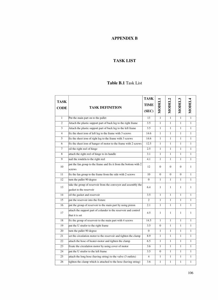
106
APPENDIX B
TASK LIST
Table B.1 Task List
TASK
CODE TASK DEFINITION
TASK
TIME
(SEC) MO
DE
L1
MO
DE
L2
MO
DE
L3
MO
DE
L4
1 Put the main part on to the pallet 13 1 1 1 1
2 Attach the plastic support part of back leg to the right frame 3.5 1 1 1 1
3 Attach the plastic support part of back leg to the left frame 3.5 1 1 1 1
4 fix the sheet iron of left leg to the frame with 3 screws 14.6 1 1 1 1
5 fix the sheet iron of right leg to the frame with 3 screws 14.6 1 1 1 1
6 fix the sheet iron of hanger of motor to the frame with 2 screws 12.5 1 1 1 1
7 oil the right reel of hinge 2.5 1 1 1 1
8 attach the right reel of hinge to its handle 3.1 1 1 1 1
9 nail the rondela to the right reel 4.1 1 1 1 1
10 put the fan group to the frame and fix it from the bottom with 2
screws 12 0 0 0 1
11 fix the fan group to the frame from the side with 2 screws 10 0 0 0 1
12 turn the pallet 90 degree 0 1 1 1 1
13 take the group of reservoir from the conveyor and assembly the
gasket to the reservoir 6.4 1 1 1 1
14 oil the gasket and reservoir 3.5 1 1 1 1
15 put the reservoir into the fixture 2 1 1 1 1
16 put the group of reservoir to the main part by using piston 2.1 1 1 1 1
17 attach the support part of colander to the reservoir and control
that it is set 4.5 1 1 1 1
18 fix the group of reservoir to the main part with 4 screws 14.5 1 1 1 1
19 put the U strafor to the right frame 3.5 0 1 1 1
20 turn the pallet 90 degree 0 1 1 1 1
21 set the circulation motor to the reservoir and tighten the clamp 8.9 1 1 1 1
22 attach the hose of heater-motor and tighten the clamp 6.5 1 1 1 1
23 fixate the circulation motor by using cover of motor 3.6 1 1 1 1
24 put the U strafor to the left frame 3.5 0 1 1 1
25 attach the long hose (having string) to the valve (3 outlets) 4 1 1 1 1
26 tighten the clamp which is attached to the hose (having string) 3.6 1 1 1 1
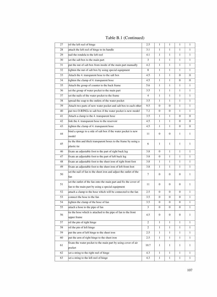
107
Table B.1 (Continued)
27 oil the left reel of hinge 2.5 1 1 1 1
28 attach the left reel of hinge to its handle 3.1 1 1 1 1
29 nail the rondela to the left reel 4.1 1 1 1 1
30 set the salt box to the main part 3 1 1 1 1
31 put the nut of salt box from inside of the main part manually 4.2 1 1 1 1
32 tighten the nut of salt box by using special equipment 8 1 1 1 1
33 Attach the 4. transparent hose to the salt box 4.5 1 1 0 0
34 tighten the clamp of 4. transparent hose 4.5 1 1 0 0
35 Attach the group of counter to the back frame 5.6 1 1 1 1
36 set the group of water pocket to the main part 3.5 1 1 1 1
37 set the nails of the water pocket to the frame 4 1 1 1 1
38 spread the soap to the outlets of the water pocket 3.5 1 1 1 1
39 Attach two parts of new water pocket and salt box to each other 9.5 0 0 1 1
40 put two O-RINGs to salt box if the water pocket is new model 7.2 0 0 1 1
41 Attach a clamp to the 4. transparent hose 3.5 1 1 0 0
42 link the 4. transparent hose to the reservoir 4.5 1 1 0 0
43 tighten the clamp of 4. transparent hose 4.5 1 1 0 0
44 bind a sponge to a side of salt box if the water pocket is new
model 11 0 0 1 1
45 tie the thin and thick transparent hoses to the frame by using a
plastic tie 6 1 1 1 1
46 fixate an adjustable foot to the part of right back leg 3.8 0 1 1 1
47 fixate an adjustable foot to the part of left back leg 3.8 0 1 1 1
48 fixate an adjustable foot to the sheet iron of right front foot 3.8 1 1 1 1
49 fixate an adjustable foot to the sheet iron of left front foot 3.8 1 1 1 1
50 set the nail of fan to the sheet iron and adjust the outlet of the
fan 7 0 0 0 1
51 set the outlet of the fan onto the main part and fix the cover of
fan to the main part by using a special equipment 11 0 0 0 1
52 attach a clamp to the hose which will be connected to the fan 2.5 0 0 0 1
53 connect the hose to the fan 3.5 0 0 0 1
54 tighten the clamp of the hose of fan 3.5 0 0 0 1
55 attach a hose to the pipe of fan 3 0 0 0 1
56 tie the hose which is attached to the pipe of fan to the front
upper frame 4.5 0 0 0 1
57 oil the pin of right hinge 2 1 1 1 1
58 oil the pin of left hinge 2 1 1 1 1
59 put the arm of left hinge to the sheet iron 2.5 1 1 1 1
60 put the arm of right hinge to the sheet iron 2.5 1 1 1 1
61 fixate the water pocket to the main part by using cover of air
pocket 10.7 1 1 1 1
62 set a string to the right reel of hinge 4.3 1 1 1 1
63 set a string to the left reel of hinge 4.3 1 1 1 1

108
Table B.1 (Continued)
64 attach the group of pipe of upper spray to the main part 5.9 1 0 0 0
65 attach the group of upper spray to the main part and fix it 4.9 0 1 1 1
66 set the sheet iron of left rail to the reels 2.9 1 1 1 1
67 set the sheet iron of right rail to the reels 2.9 1 1 1 1
68 attach the cover of right rail from the back 4 1 1 1 1
69 attach the cover of left rail from the back 4 1 1 1 1
70 attach the bottom propeller to the pump reservoir 2.7 1 1 1 1
71 peel the foil which is bind to the frame 5 1 1 1 1
72 erect the main part C 1 1 1 1
73 set the handle of motor card to the main part 5.5 0 0 0 1
74 attach two screws to the handle of motor card 9.3 0 0 0 1
75 attach a screw to the group 4.2 1 1 1 0
76 attach the part of the lock 4.5 1 1 1 1
77 spread the soap to the sheet iron of gasket 3.9 1 1 1 1
78 attach two covers to the sheet iron of gasket 8 1 1 1 1
79 attach the gasket of the lid to its sheet iron manually 21 1 1 1 1
80 tighten the bottom part of sheet iron of gasket of the lid by
using hammer 1.5 1 1 1 1
81 set the handle of spring to the right frame 2.5 1 1 1 1
82 attach the spring to the right spring handle 1.2 1 1 1 1
83 take the group of inner lid from the conveyor and put it onto the
arms of hinge 6.1 1 1 1 1
84 fix the left arm of hinge to the inner lid with 2 screws 7.8 1 1 1 1
85 fix the right arm of hinge to the inner lid with 2 screws 7.8 1 1 1 1
86 close the inner lid which is screwed 2.5 1 1 1 1
87 stretch the right spring and connect it to the string 4.2 1 1 1 1
88 stretch the left spring and connect it to the string 4.2 1 1 1 1
89 set the handle of spring to the left frame 2.5 1 1 1 1
90 attach the spring to the left spring handle 1.8 1 1 1 1
91 put the support sheet iron onto the arms of hinge 2.3 1 1 1 1
92 fix the support sheet iron to the arms of hinge with a screw 3.7 1 1 1 1
93 fix the support sheet iron to the arms of hinge with a screw 3.7 1 1 1 1
94 fix the support sheet iron with a screw 3.7 1 1 1 1
95 fix the cable of earth to the support sheet iron with a screw 5.3 1 1 1 1
96 pass the hose of flusher from the hook of heater-reservoir hose 2 1 1 1 1
97 attach the other end of the hose of flusher to the buoy 7.4 1 1 1 1
98 tie the 2. hose of flusher to the buoy 5.5 1 1 1 1
99 attach the polisher switch to the detergent box 3.8 1 1 1 1
100 attach a cable to the detergent box 3.9 1 1 0 0
101 attach a isolater to the detergent box cable 3 1 1 0 0
102 attach a cable to the detergent box 3.9 1 1 1 0
103 set the support strafor to the support sheet iron 2.6 1 1 1 1
104 fix the strafor to the sheet iron by tighten the sheet iron 4.5 1 1 1 1
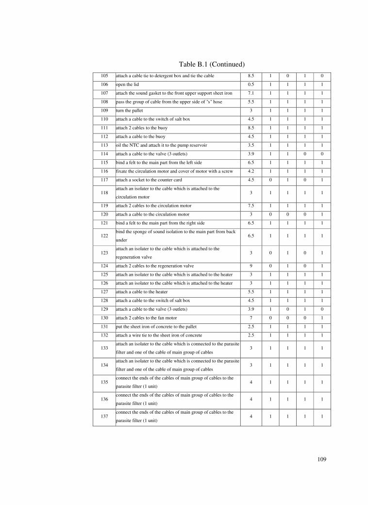
109
Table B.1 (Continued)
105 attach a cable tie to detergent box and tie the cable 8.5 1 0 1 0
106 open the lid 0.5 1 1 1 1
107 attach the sound gasket to the front upper support sheet iron 7.1 1 1 1 1
108 pass the group of cable from the upper side of "s" hose 5.5 1 1 1 1
109 turn the pallet 3 1 1 1 1
110 attach a cable to the switch of salt box 4.5 1 1 1 1
111 attach 2 cables to the buoy 8.5 1 1 1 1
112 attach a cable to the buoy 4.5 1 1 1 1
113 oil the NTC and attach it to the pump reservoir 3.5 1 1 1 1
114 attach a cable to the valve (3 outlets) 3.9 1 1 0 0
115 bind a felt to the main part from the left side 6.5 1 1 1 1
116 fixate the circulation motor and cover of motor with a screw 4.2 1 1 1 1
117 attach a socket to the counter card 4.5 0 1 0 1
118 attach an isolater to the cable which is attached to the
circulation motor 3 1 1 1 1
119 attach 2 cables to the circulation motor 7.5 1 1 1 1
120 attach a cable to the circulation motor 3 0 0 0 1
121 bind a felt to the main part from the right side 6.5 1 1 1 1
122 bind the sponge of sound isolation to the main part from back
under 6.5 1 1 1 1
123 attach an isolater to the cable which is attached to the
regeneration valve 3 0 1 0 1
124 attach 2 cables to the regeneration valve 9 0 1 0 1
125 attach an isolater to the cable which is attached to the heater 3 1 1 1 1
126 attach an isolater to the cable which is attached to the heater 3 1 1 1 1
127 attach a cable to the heater 5.5 1 1 1 1
128 attach a cable to the switch of salt box 4.5 1 1 1 1
129 attach a cable to the valve (3 outlets) 3.9 1 0 1 0
130 attach 2 cables to the fan motor 7 0 0 0 1
131 put the sheet iron of concrete to the pallet 2.5 1 1 1 1
132 attach a wire tie to the sheet iron of concrete 2.5 1 1 1 1
133 attach an isolater to the cable which is connected to the parasite
filter and one of the cable of main group of cables 3 1 1 1 1
134 attach an isolater to the cable which is connected to the parasite
filter and one of the cable of main group of cables 3 1 1 1 1
135 connect the ends of the cables of main group of cables to the
parasite filter (1 unit) 4 1 1 1 1
136 connect the ends of the cables of main group of cables to the
parasite filter (1 unit) 4 1 1 1 1
137 connect the ends of the cables of main group of cables to the
parasite filter (1 unit) 4 1 1 1 1
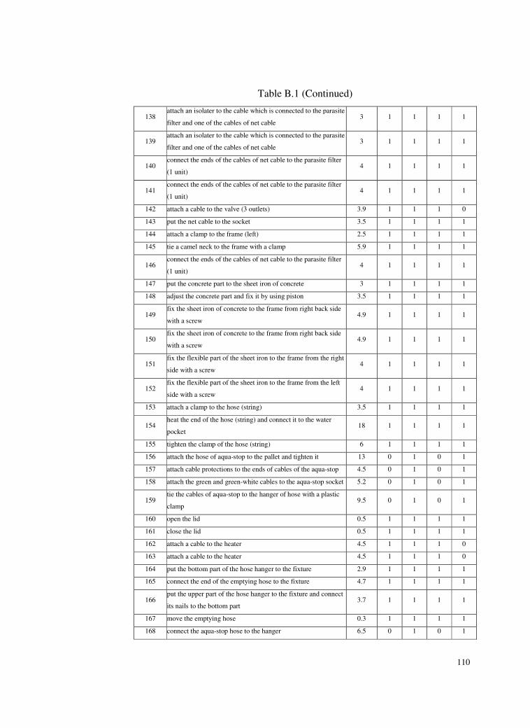
110
Table B.1 (Continued)
138 attach an isolater to the cable which is connected to the parasite
filter and one of the cables of net cable 3 1 1 1 1
139 attach an isolater to the cable which is connected to the parasite
filter and one of the cables of net cable 3 1 1 1 1
140 connect the ends of the cables of net cable to the parasite filter
(1 unit) 4 1 1 1 1
141 connect the ends of the cables of net cable to the parasite filter
(1 unit) 4 1 1 1 1
142 attach a cable to the valve (3 outlets) 3.9 1 1 1 0
143 put the net cable to the socket 3.5 1 1 1 1
144 attach a clamp to the frame (left) 2.5 1 1 1 1
145 tie a camel neck to the frame with a clamp 5.9 1 1 1 1
146 connect the ends of the cables of net cable to the parasite filter
(1 unit) 4 1 1 1 1
147 put the concrete part to the sheet iron of concrete 3 1 1 1 1
148 adjust the concrete part and fix it by using piston 3.5 1 1 1 1
149 fix the sheet iron of concrete to the frame from right back side
with a screw 4.9 1 1 1 1
150 fix the sheet iron of concrete to the frame from right back side
with a screw 4.9 1 1 1 1
151 fix the flexible part of the sheet iron to the frame from the right
side with a screw 4 1 1 1 1
152 fix the flexible part of the sheet iron to the frame from the left
side with a screw 4 1 1 1 1
153 attach a clamp to the hose (string) 3.5 1 1 1 1
154 heat the end of the hose (string) and connect it to the water
pocket 18 1 1 1 1
155 tighten the clamp of the hose (string) 6 1 1 1 1
156 attach the hose of aqua-stop to the pallet and tighten it 13 0 1 0 1
157 attach cable protections to the ends of cables of the aqua-stop 4.5 0 1 0 1
158 attach the green and green-white cables to the aqua-stop socket 5.2 0 1 0 1
159 tie the cables of aqua-stop to the hanger of hose with a plastic
clamp 9.5 0 1 0 1
160 open the lid 0.5 1 1 1 1
161 close the lid 0.5 1 1 1 1
162 attach a cable to the heater 4.5 1 1 1 0
163 attach a cable to the heater 4.5 1 1 1 0
164 put the bottom part of the hose hanger to the fixture 2.9 1 1 1 1
165 connect the end of the emptying hose to the fixture 4.7 1 1 1 1
166 put the upper part of the hose hanger to the fixture and connect
its nails to the bottom part 3.7 1 1 1 1
167 move the emptying hose 0.3 1 1 1 1
168 connect the aqua-stop hose to the hanger 6.5 0 1 0 1
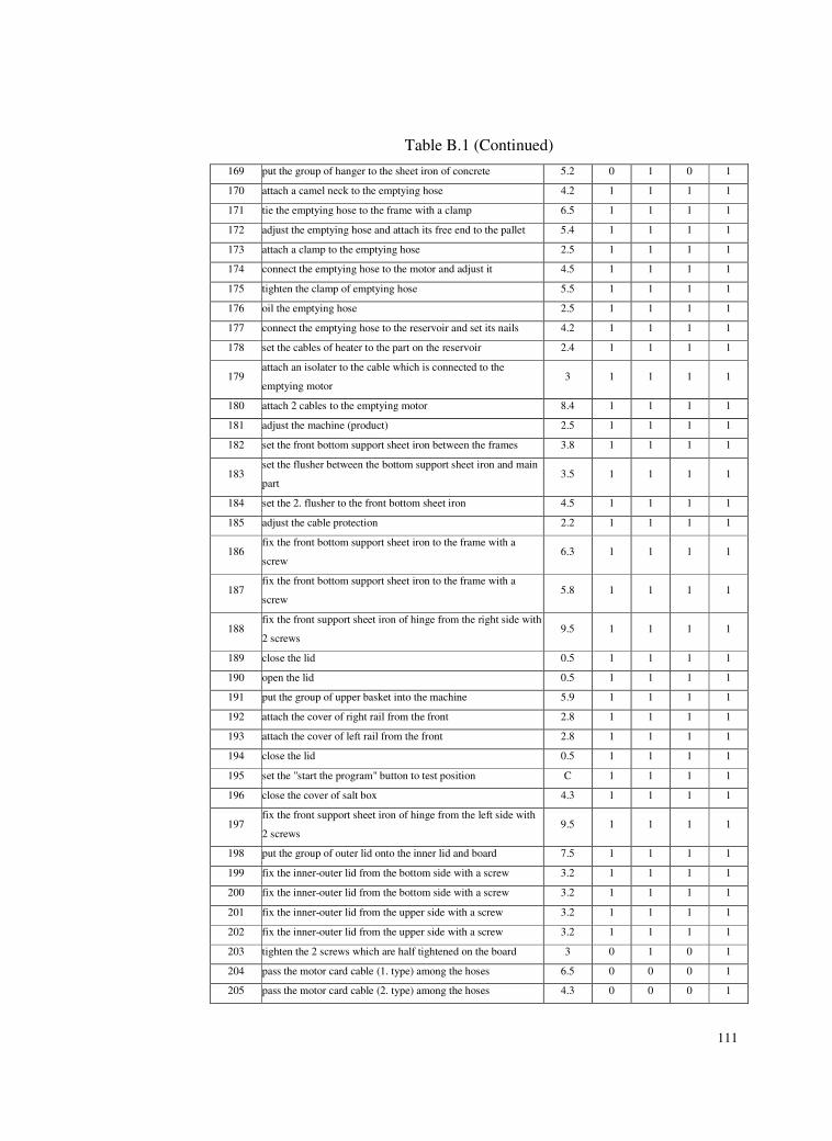
111
Table B.1 (Continued)
169 put the group of hanger to the sheet iron of concrete 5.2 0 1 0 1
170 attach a camel neck to the emptying hose 4.2 1 1 1 1
171 tie the emptying hose to the frame with a clamp 6.5 1 1 1 1
172 adjust the emptying hose and attach its free end to the pallet 5.4 1 1 1 1
173 attach a clamp to the emptying hose 2.5 1 1 1 1
174 connect the emptying hose to the motor and adjust it 4.5 1 1 1 1
175 tighten the clamp of emptying hose 5.5 1 1 1 1
176 oil the emptying hose 2.5 1 1 1 1
177 connect the emptying hose to the reservoir and set its nails 4.2 1 1 1 1
178 set the cables of heater to the part on the reservoir 2.4 1 1 1 1
179 attach an isolater to the cable which is connected to the
emptying motor 3 1 1 1 1
180 attach 2 cables to the emptying motor 8.4 1 1 1 1
181 adjust the machine (product) 2.5 1 1 1 1
182 set the front bottom support sheet iron between the frames 3.8 1 1 1 1
183 set the flusher between the bottom support sheet iron and main
part 3.5 1 1 1 1
184 set the 2. flusher to the front bottom sheet iron 4.5 1 1 1 1
185 adjust the cable protection 2.2 1 1 1 1
186 fix the front bottom support sheet iron to the frame with a
screw 6.3 1 1 1 1
187 fix the front bottom support sheet iron to the frame with a
screw 5.8 1 1 1 1
188 fix the front support sheet iron of hinge from the right side with
2 screws 9.5 1 1 1 1
189 close the lid 0.5 1 1 1 1
190 open the lid 0.5 1 1 1 1
191 put the group of upper basket into the machine 5.9 1 1 1 1
192 attach the cover of right rail from the front 2.8 1 1 1 1
193 attach the cover of left rail from the front 2.8 1 1 1 1
194 close the lid 0.5 1 1 1 1
195 set the "start the program" button to test position C 1 1 1 1
196 close the cover of salt box 4.3 1 1 1 1
197 fix the front support sheet iron of hinge from the left side with
2 screws 9.5 1 1 1 1
198 put the group of outer lid onto the inner lid and board 7.5 1 1 1 1
199 fix the inner-outer lid from the bottom side with a screw 3.2 1 1 1 1
200 fix the inner-outer lid from the bottom side with a screw 3.2 1 1 1 1
201 fix the inner-outer lid from the upper side with a screw 3.2 1 1 1 1
202 fix the inner-outer lid from the upper side with a screw 3.2 1 1 1 1
203 tighten the 2 screws which are half tightened on the board 3 0 1 0 1
204 pass the motor card cable (1. type) among the hoses 6.5 0 0 0 1
205 pass the motor card cable (2. type) among the hoses 4.3 0 0 0 1

112
Table B.1 (Continued)
206 connect the motor card cable (1. type) and adjust it 6.5 0 0 0 1
207 operate the bottom plane robot 5.5 1 1 1 1
208 attach the part which fixates the upper plane 0 1 1 1 1
209 attach 2 L strafors to the frame 0 1 1 1 1
210 connect the buoy and bottom plane 2.1 1 1 1 1
211 fixate the bottom plane with 2 screws to the frame 10.6 1 1 1 1
212 check the cables and hoses of buoy after attaching the bottom
plane 2.1 1 1 1 1
213 attach the mistake trace paper to the lid with a magnet 2.1 1 1 1 1
214 control the 1. electrical test 1 1 1 1 1
215 connect the motor card cable (2. type) and adjust it 6.4 0 0 0 1
216 send the pallet 5.5 1 1 1 1
217 open the lid 0.5 1 1 1 1
218 open the cover of salt box 3 1 1 1 1
219 evacuate the water in the salt box with the vacuum machine 10.2 1 1 1 1
220 move the micro filter and reservoir 0 1 1 1 1
221 connect the cable of circulation motor card to the card 5.6 0 0 0 1
222 evacuate the water in the reservoir with the vacuum machine 6.8 1 1 1 1
223 close the cover of salt box 0 1 1 1 1
224 put the colander into the reservoir 2.1 1 1 1 1
225 put the micro filter to the colander and tighten it 2.1 1 1 1 1
226 bind a sticker to the cover of salt box 5.8 1 1 1 1
227 adjust the tuning screw in the water pocket by using
screwdriver 3.5 1 1 1 1
228 close the lid 0.5 1 1 1 1
229 put a felt on to the main body 3.5 1 1 1 1
230 ravel the water entry hose from the pallet 6.8 1 1 1 1
231 ravel the emptying hose from the pallet 0.8 1 1 1 1
232 tie the water entry and emptying hoses according to the figure 5.1 1 1 1 1
233 tie the water entry and emptying hoses with a clamp 3.9 1 1 1 1
234 put a felt on to the machine 4.1 0 0 0 1
235 attach a clamp to the right frame 2.5 1 1 1 1
236 set a long starafor to the right back frame 4.7 1 1 1 1
237 set a long starafor to the left back frame 4.7 1 1 1 1
238 attach the sound gasket to the left side by using the equipment 7.8 0 0 1 1
239 attach a strafor to the left back side of main body 2.9 1 1 1 1
240 attach the left side plane and fix it with 2 screws 15 1 1 1 1
241 put 2 white stopper to the left side plane 4.1 1 1 1 1
242 attach the centralize part of inner lid (left and right) 8 1 1 1 1
243 attach the sound gasket to the right side by using the equipment 7.8 0 0 1 1
244 attach a strafor to the right back side of main body 2.9 1 1 1 1
245 attach the right side plane and fix it with 2 screws 15 1 1 1 1
246 put 2 white stopper to the right side plane 4.1 1 1 1 1
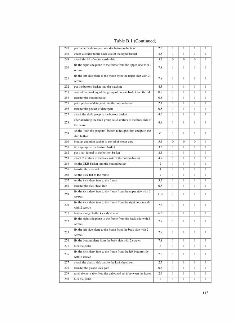
113
Table B.1 (Continued)
247 put the left side support starafor between the felts 2.3 1 1 1 1
248 attach a strafor to the back side of the upper basket 3.5 1 1 1 1
249 attach the lid of motor card cable 5.7 0 0 0 1
250 fix the right side plane to the frame from the upper side with 2
screws 7.8 1 1 1 1
251 fix the left side plane to the frame from the upper side with 2
screws 7.8 1 1 1 1
252 put the bottom basket into the machine 4.3 1 1 1 1
253 control the working of the group of bottom basket and the lid 0.8 1 1 1 1
254 transfer the bottom basket 0.5 1 1 1 1
255 put a pocket of detergent into the bottom basket 2.1 1 1 1 1
256 transfer the pocket of detergent 0.5 1 1 1 1
257 attach the shelf group to the bottom basket 4.5 1 1 1 1
258 after attaching the shelf group set 2 strafors to the back side of
the basket 4.9 1 1 1 1
259 set the "start the program" button to test position and push the
start button C 1 1 1 1
260 bind an attention sticker to the lid of motor card 5.5 0 0 0 1
261 tie a sponge to the bottom basket 3.5 1 1 1 1
262 put a salt funnel to the bottom basket 2.1 1 1 1 1
263 attach 2 strafors to the back side of the bottom basket 4.9 1 1 1 1
264 set the CKB basket into the bottom basket 2 1 1 1 1
265 transfer the material 1 1 1 1 1
266 set the kick felt to the frame 9 1 1 1 1
267 set the kick sheet iron to the frame 3.7 1 1 1 1
268 transfer the kick sheet iron 0.5 1 1 1 1
269 fix the kick sheet iron to the frame from the upper side with 2
screws 11.6 1 1 1 1
270 fix the kick sheet iron to the frame from the right bottom side
with 2 screws 7.8 1 1 1 1
271 bind a sponge to the kick sheet iron 6.5 1 1 1 1
272 fix the right side plane to the frame from the back side with 2
screws 7.8 1 1 1 1
273 fix the left side plane to the frame from the back side with 2
screws 7.8 1 1 1 1
274 fix the bottom plane from the back side with 2 screws 7.8 1 1 1 1
275 turn the pallet 3 1 1 1 1
276 fix the kick sheet iron to the frame from the left bottom side
with 2 screws 7.8 1 1 1 1
277 attach the plastic kick part to the kick sheet iron 2.7 1 1 1 1
278 transfer the plastic kick part 0.5 1 1 1 1
279 ravel the net cable from the pallet and set it between the hoses 2.7 1 1 1 1
280 turn the pallet 3 1 1 1 1
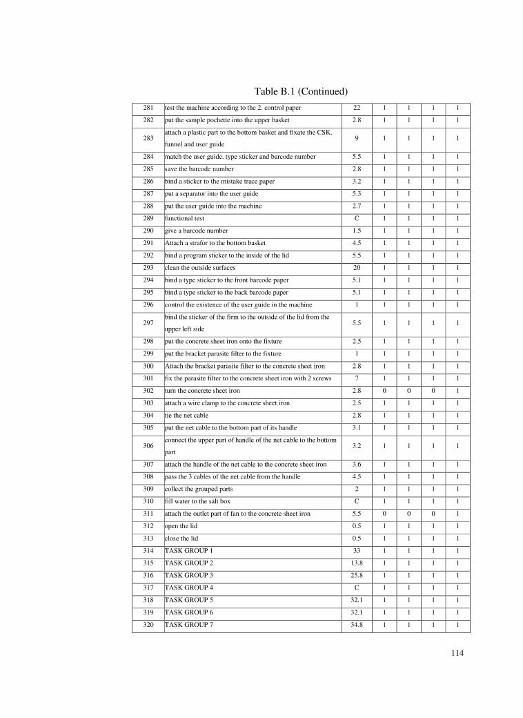
114
Table B.1 (Continued)
281 test the machine according to the 2. control paper 22 1 1 1 1
282 put the sample pochette into the upper basket 2.8 1 1 1 1
283 attach a plastic part to the bottom basket and fixate the CSK.
funnel and user guide 9 1 1 1 1
284 match the user guide. type sticker and barcode number 5.5 1 1 1 1
285 save the barcode number 2.8 1 1 1 1
286 bind a sticker to the mistake trace paper 3.2 1 1 1 1
287 put a separator into the user guide 5.3 1 1 1 1
288 put the user guide into the machine 2.7 1 1 1 1
289 functional test C 1 1 1 1
290 give a barcode number 1.5 1 1 1 1
291 Attach a strafor to the bottom basket 4.5 1 1 1 1
292 bind a program sticker to the inside of the lid 5.5 1 1 1 1
293 clean the outside surfaces 20 1 1 1 1
294 bind a type sticker to the front barcode paper 5.1 1 1 1 1
295 bind a type sticker to the back barcode paper 5.1 1 1 1 1
296 control the existence of the user guide in the machine 1 1 1 1 1
297 bind the sticker of the firm to the outside of the lid from the
upper left side 5.5 1 1 1 1
298 put the concrete sheet iron onto the fixture 2.5 1 1 1 1
299 put the bracket parasite filter to the fixture 1 1 1 1 1
300 Attach the bracket parasite filter to the concrete sheet iron 2.8 1 1 1 1
301 fix the parasite filter to the concrete sheet iron with 2 screws 7 1 1 1 1
302 turn the concrete sheet iron 2.8 0 0 0 1
303 attach a wire clamp to the concrete sheet iron 2.5 1 1 1 1
304 tie the net cable 2.8 1 1 1 1
305 put the net cable to the bottom part of its handle 3.1 1 1 1 1
306 connect the upper part of handle of the net cable to the bottom
part 3.2 1 1 1 1
307 attach the handle of the net cable to the concrete sheet iron 3.6 1 1 1 1
308 pass the 3 cables of the net cable from the handle 4.5 1 1 1 1
309 collect the grouped parts 2 1 1 1 1
310 fill water to the salt box C 1 1 1 1
311 attach the outlet part of fan to the concrete sheet iron 5.5 0 0 0 1
312 open the lid 0.5 1 1 1 1
313 close the lid 0.5 1 1 1 1
314 TASK GROUP 1 33 1 1 1 1
315 TASK GROUP 2 13.8 1 1 1 1
316 TASK GROUP 3 25.8 1 1 1 1
317 TASK GROUP 4 C 1 1 1 1
318 TASK GROUP 5 32.1 1 1 1 1
319 TASK GROUP 6 32.1 1 1 1 1
320 TASK GROUP 7 34.8 1 1 1 1

115
Table B.1 (Continued)
321 TASK GROUP 8 33 1 1 1 1
322 TASK GROUP 9 34.5 1 1 1 1
323 TASK GROUP 10 4.9 1 1 1 1
Note: The number 1 in model columns shows that corresponding model
includes the corresponding task. and the number 0 in model columns shows
that corresponding model does not include the corresponding task
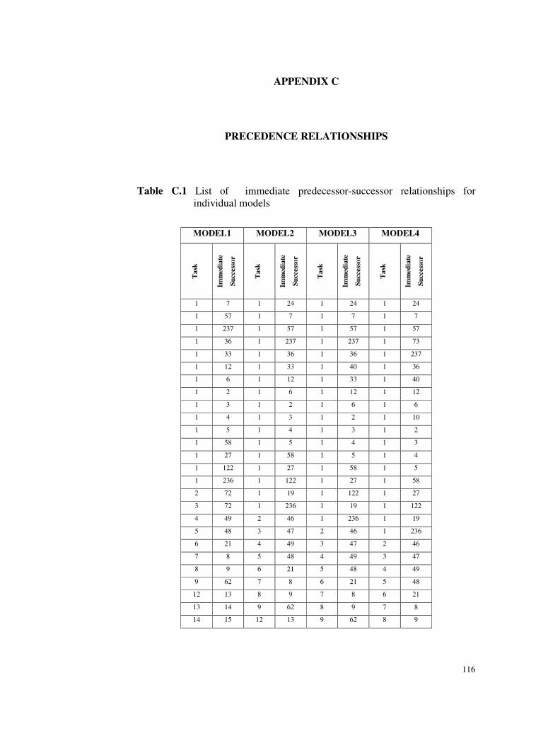
116
APPENDIX C
PRECEDENCE RELATIONSHIPS
Table C.1 List of immediate predecessor-successor relationships for
individual models
MODEL1 MODEL2 MODEL3 MODEL4
Task
Im
med
iate
Su
ccesso
r
Task
Im
med
iate
Su
ccesso
r
Task
Im
med
iate
Su
ccesso
r
Task
Im
med
iate
Su
ccesso
r
1 7 1 24 1 24 1 24
1 57 1 7 1 7 1 7
1 237 1 57 1 57 1 57
1 36 1 237 1 237 1 73
1 33 1 36 1 36 1 237
1 12 1 33 1 40 1 36
1 6 1 12 1 33 1 40
1 2 1 6 1 12 1 12
1 3 1 2 1 6 1 6
1 4 1 3 1 2 1 10
1 5 1 4 1 3 1 2
1 58 1 5 1 4 1 3
1 27 1 58 1 5 1 4
1 122 1 27 1 58 1 5
1 236 1 122 1 27 1 58
2 72 1 19 1 122 1 27
3 72 1 236 1 19 1 122
4 49 2 46 1 236 1 19
5 48 3 47 2 46 1 236
6 21 4 49 3 47 2 46
7 8 5 48 4 49 3 47
8 9 6 21 5 48 4 49
9 62 7 8 6 21 5 48
12 13 8 9 7 8 6 21
13 14 9 62 8 9 7 8
14 15 12 13 9 62 8 9
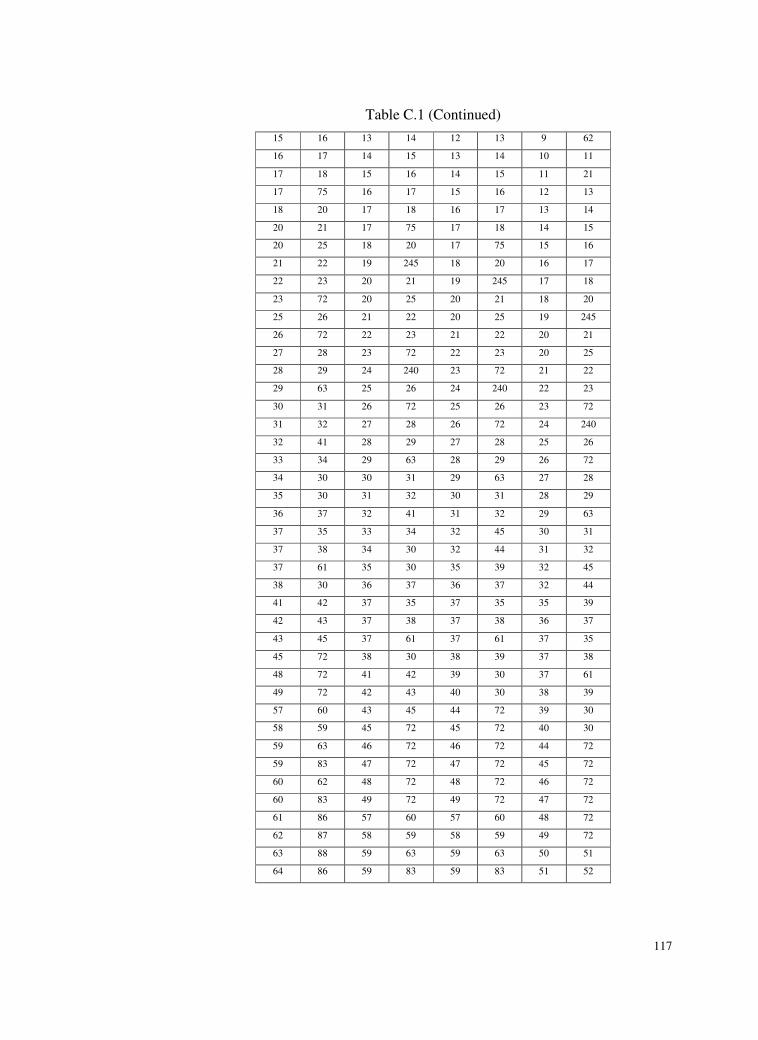
117
Table C.1 (Continued)
15 16 13 14 12 13 9 62
16 17 14 15 13 14 10 11
17 18 15 16 14 15 11 21
17 75 16 17 15 16 12 13
18 20 17 18 16 17 13 14
20 21 17 75 17 18 14 15
20 25 18 20 17 75 15 16
21 22 19 245 18 20 16 17
22 23 20 21 19 245 17 18
23 72 20 25 20 21 18 20
25 26 21 22 20 25 19 245
26 72 22 23 21 22 20 21
27 28 23 72 22 23 20 25
28 29 24 240 23 72 21 22
29 63 25 26 24 240 22 23
30 31 26 72 25 26 23 72
31 32 27 28 26 72 24 240
32 41 28 29 27 28 25 26
33 34 29 63 28 29 26 72
34 30 30 31 29 63 27 28
35 30 31 32 30 31 28 29
36 37 32 41 31 32 29 63
37 35 33 34 32 45 30 31
37 38 34 30 32 44 31 32
37 61 35 30 35 39 32 45
38 30 36 37 36 37 32 44
41 42 37 35 37 35 35 39
42 43 37 38 37 38 36 37
43 45 37 61 37 61 37 35
45 72 38 30 38 39 37 38
48 72 41 42 39 30 37 61
49 72 42 43 40 30 38 39
57 60 43 45 44 72 39 30
58 59 45 72 45 72 40 30
59 63 46 72 46 72 44 72
59 83 47 72 47 72 45 72
60 62 48 72 48 72 46 72
60 83 49 72 49 72 47 72
61 86 57 60 57 60 48 72
62 87 58 59 58 59 49 72
63 88 59 63 59 63 50 51
64 86 59 83 59 83 51 52
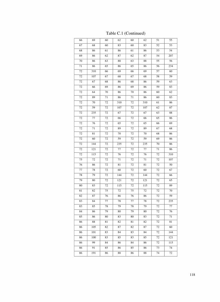
118
Table C.1 (Continued)
66 69 60 62 60 62 51 55
67 68 60 83 60 83 52 53
68 86 61 86 61 86 53 54
69 86 62 87 62 87 54 207
70 86 63 88 63 88 55 56
71 86 65 86 65 86 56 234
72 310 66 69 66 69 57 60
72 107 67 68 67 68 58 59
72 67 68 86 68 86 59 63
72 66 69 86 69 86 59 83
72 64 70 86 70 86 60 62
72 89 71 86 71 86 60 83
72 70 72 310 72 310 61 86
72 59 72 107 72 107 62 87
72 235 72 67 72 67 63 88
72 77 72 66 72 66 65 86
72 76 72 65 72 65 66 69
72 71 72 89 72 89 67 68
72 81 72 70 72 70 68 86
72 60 72 59 72 59 69 86
72 144 72 235 72 235 70 86
72 121 72 77 72 77 71 86
72 115 72 76 72 76 72 310
75 72 72 71 72 71 72 107
76 86 72 81 72 81 72 50
77 78 72 60 72 60 72 67
78 79 72 144 72 144 72 66
79 80 72 121 72 121 72 65
80 83 72 115 72 115 72 89
81 82 75 72 75 72 72 70
82 87 76 86 76 86 72 59
83 84 77 78 77 78 72 235
83 85 78 79 78 79 72 77
84 86 79 80 79 80 72 76
85 86 80 83 80 83 72 71
86 88 81 82 81 82 72 81
86 105 82 87 82 87 72 60
86 101 83 84 83 84 72 144
86 100 83 85 83 85 72 121
86 99 84 86 84 86 72 115
86 91 85 86 85 86 73 74
86 191 86 88 86 88 74 72
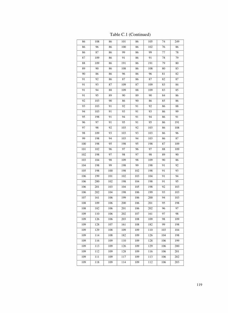
119
Table C.1 (Continued)
86 108 86 101 86 105 74 249
86 96 86 100 86 102 76 86
86 87 86 99 86 99 77 78
87 109 86 91 86 91 78 79
88 109 86 191 86 191 79 80
89 90 86 108 86 108 80 83
90 86 86 96 86 96 81 82
91 92 86 87 86 87 82 87
91 93 87 109 87 109 83 84
91 94 88 109 88 109 83 85
91 95 89 90 89 90 84 86
92 103 90 86 90 86 85 86
93 103 91 92 91 92 86 88
94 103 91 93 91 93 86 99
95 198 91 94 91 94 86 91
96 97 91 95 91 95 86 191
97 98 92 103 92 103 86 108
98 109 93 103 93 103 86 96
99 198 94 103 94 103 86 87
100 198 95 198 95 198 87 109
101 102 96 97 96 97 88 109
102 198 97 98 97 98 89 90
103 104 98 109 98 109 90 86
104 198 99 198 99 198 91 92
105 198 100 198 102 198 91 93
106 199 101 102 103 104 91 94
106 200 102 198 104 198 91 95
106 201 103 104 105 198 92 103
106 202 104 198 106 199 93 103
107 161 106 199 106 200 94 103
108 109 106 200 106 201 95 198
108 182 106 201 106 202 96 97
109 110 106 202 107 161 97 98
109 126 106 203 108 109 98 109
109 128 107 161 108 182 99 198
109 129 108 109 109 110 103 104
109 114 108 182 109 126 104 198
109 116 109 110 109 128 106 199
109 113 109 126 109 129 106 200
109 112 109 128 109 116 106 201
109 111 109 117 109 113 106 202
109 118 109 114 109 112 106 203

120
Table C.1 (Continued)
109 125 109 116 109 111 107 161
109 142 109 113 109 118 108 109
110 131 109 112 109 125 108 182
111 131 109 111 109 142 109 205
112 131 109 118 110 131 109 204
113 131 109 123 111 131 109 120
114 131 109 125 112 131 109 130
115 239 109 142 113 131 109 110
115 247 110 131 115 238 109 126
115 244 111 131 115 239 109 128
116 131 112 131 115 247 109 117
118 119 113 131 115 243 109 116
119 131 114 131 115 244 109 113
121 239 115 239 116 131 109 112
121 247 115 244 118 119 109 111
121 244 115 247 119 131 109 118
122 207 116 131 121 238 109 123
125 127 117 131 121 239 109 125
126 131 118 119 121 247 110 131
127 131 119 131 121 243 111 131
128 131 121 239 121 244 112 131
129 131 121 244 122 207 113 131
131 132 121 247 125 127 115 234
131 133 122 207 126 131 116 131
131 134 123 124 127 131 117 131
131 135 124 131 128 131 118 119
131 138 125 127 129 131 119 131
131 139 126 131 131 132 120 221
131 146 127 131 131 133 121 234
132 171 128 131 131 134 122 207
133 136 131 132 131 135 123 124
134 137 131 133 131 138 124 131
135 147 131 134 131 139 125 127
136 147 131 135 131 146 126 131
137 147 131 138 132 171 127 131
138 140 131 139 133 136 128 131
139 141 131 146 134 137 130 131
140 147 132 171 135 147 131 132
141 147 133 136 136 147 131 133
142 131 134 137 137 147 131 134
143 195 135 147 138 140 131 135
144 145 136 147 139 141 131 138
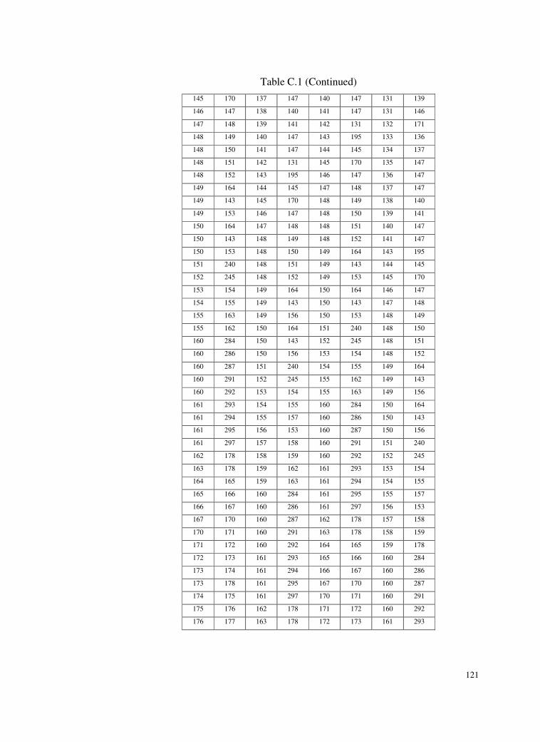
121
Table C.1 (Continued)
145 170 137 147 140 147 131 139
146 147 138 140 141 147 131 146
147 148 139 141 142 131 132 171
148 149 140 147 143 195 133 136
148 150 141 147 144 145 134 137
148 151 142 131 145 170 135 147
148 152 143 195 146 147 136 147
149 164 144 145 147 148 137 147
149 143 145 170 148 149 138 140
149 153 146 147 148 150 139 141
150 164 147 148 148 151 140 147
150 143 148 149 148 152 141 147
150 153 148 150 149 164 143 195
151 240 148 151 149 143 144 145
152 245 148 152 149 153 145 170
153 154 149 164 150 164 146 147
154 155 149 143 150 143 147 148
155 163 149 156 150 153 148 149
155 162 150 164 151 240 148 150
160 284 150 143 152 245 148 151
160 286 150 156 153 154 148 152
160 287 151 240 154 155 149 164
160 291 152 245 155 162 149 143
160 292 153 154 155 163 149 156
161 293 154 155 160 284 150 164
161 294 155 157 160 286 150 143
161 295 156 153 160 287 150 156
161 297 157 158 160 291 151 240
162 178 158 159 160 292 152 245
163 178 159 162 161 293 153 154
164 165 159 163 161 294 154 155
165 166 160 284 161 295 155 157
166 167 160 286 161 297 156 153
167 170 160 287 162 178 157 158
170 171 160 291 163 178 158 159
171 172 160 292 164 165 159 178
172 173 161 293 165 166 160 284
173 174 161 294 166 167 160 286
173 178 161 295 167 170 160 287
174 175 161 297 170 171 160 291
175 176 162 178 171 172 160 292
176 177 163 178 172 173 161 293

122
Table C.1 (Continued)
177 179 164 165 173 174 161 294
178 173 164 168 173 178 161 295
178 181 165 166 174 175 161 297
179 180 166 167 175 176 164 165
180 181 167 169 176 177 164 168
181 207 168 166 177 179 165 166
182 183 169 170 178 173 166 167
182 184 170 171 178 181 167 169
183 185 171 172 179 180 168 166
184 185 172 173 180 181 169 170
185 186 173 174 181 207 170 171
185 187 173 178 182 183 171 172
186 188 174 175 182 184 172 173
186 197 175 176 183 185 173 174
187 188 176 177 184 185 173 178
187 197 177 179 185 186 174 175
188 198 178 173 185 187 175 176
189 207 178 181 186 188 176 177
189 213 179 180 186 197 177 179
190 252 180 181 187 188 178 173
191 192 181 207 187 197 178 181
191 193 182 183 188 198 179 180
192 312 182 184 189 207 180 181
192 160 183 185 189 213 181 207
192 248 184 185 190 252 182 183
193 160 185 186 191 192 182 184
193 312 185 187 191 193 183 185
194 312 186 188 192 312 184 185
194 160 186 197 192 160 185 186
195 214 187 188 192 248 185 187
196 289 187 197 193 160 186 188
197 198 188 198 193 312 186 197
198 106 189 207 194 312 187 188
198 266 189 213 194 160 187 197
199 189 190 252 195 214 188 198
200 189 191 192 196 289 189 207
201 189 191 193 197 198 189 213
202 189 192 312 198 106 190 252
206 131 192 160 198 266 191 192
207 208 192 248 199 189 191 193
207 209 193 312 200 189 192 312
208 210 193 160 201 189 192 160

123
Table C.1 (Continued)
209 210 194 312 202 189 192 248
210 211 194 160 207 208 193 160
211 212 195 214 207 209 193 312
212 216 196 289 208 210 194 312
213 214 197 198 209 210 194 160
214 216 198 106 210 211 195 214
216 289 198 266 211 212 196 289
216 239 199 189 212 216 197 198
216 247 200 189 213 214 198 106
216 244 201 189 214 216 198 266
217 218 202 189 216 289 199 189
217 220 203 189 216 238 200 189
217 227 207 208 216 239 201 189
218 219 207 209 216 247 202 189
218 226 208 210 216 243 203 189
219 223 209 210 216 244 204 206
220 222 210 211 217 218 205 215
222 224 211 212 217 220 206 131
223 228 212 216 217 227 207 208
224 225 213 214 218 219 207 209
225 228 214 216 218 226 208 210
226 228 216 289 219 223 209 210
227 228 216 239 220 222 210 211
228 229 216 244 222 224 211 212
228 190 216 247 223 228 212 216
229 230 217 218 224 225 213 214
229 231 217 220 225 228 214 216
230 232 217 227 226 228 215 131
230 233 218 219 227 228 216 289
231 232 218 226 228 229 216 234
231 233 219 223 228 190 217 218
232 279 220 222 229 230 217 220
233 279 222 224 229 231 217 227
235 232 223 228 230 232 218 219
235 233 224 225 230 233 218 226
236 245 225 228 231 232 219 223
237 240 226 228 231 233 220 222
239 240 227 228 232 279 221 131
240 241 228 229 233 279 222 224
241 242 228 190 235 232 223 228
241 251 229 230 235 233 224 225
242 275 229 231 236 245 225 228
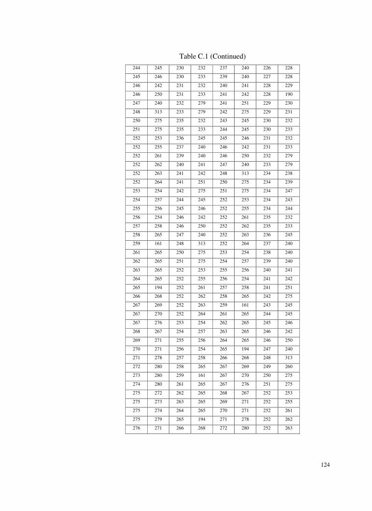
124
Table C.1 (Continued)
244 245 230 232 237 240 226 228
245 246 230 233 239 240 227 228
246 242 231 232 240 241 228 229
246 250 231 233 241 242 228 190
247 240 232 279 241 251 229 230
248 313 233 279 242 275 229 231
250 275 235 232 243 245 230 232
251 275 235 233 244 245 230 233
252 253 236 245 245 246 231 232
252 255 237 240 246 242 231 233
252 261 239 240 246 250 232 279
252 262 240 241 247 240 233 279
252 263 241 242 248 313 234 238
252 264 241 251 250 275 234 239
253 254 242 275 251 275 234 247
254 257 244 245 252 253 234 243
255 256 245 246 252 255 234 244
256 254 246 242 252 261 235 232
257 258 246 250 252 262 235 233
258 265 247 240 252 263 236 245
259 161 248 313 252 264 237 240
261 265 250 275 253 254 238 240
262 265 251 275 254 257 239 240
263 265 252 253 255 256 240 241
264 265 252 255 256 254 241 242
265 194 252 261 257 258 241 251
266 268 252 262 258 265 242 275
267 269 252 263 259 161 243 245
267 270 252 264 261 265 244 245
267 276 253 254 262 265 245 246
268 267 254 257 263 265 246 242
269 271 255 256 264 265 246 250
270 271 256 254 265 194 247 240
271 278 257 258 266 268 248 313
272 280 258 265 267 269 249 260
273 280 259 161 267 270 250 275
274 280 261 265 267 276 251 275
275 272 262 265 268 267 252 253
275 273 263 265 269 271 252 255
275 274 264 265 270 271 252 261
275 279 265 194 271 278 252 262
276 271 266 268 272 280 252 263

125
Table C.1 (Continued)
277 312 267 269 273 280 252 264
277 160 267 270 274 280 253 254
278 277 267 276 275 272 254 257
279 280 268 267 275 273 255 256
280 275 269 271 275 274 256 254
280 312 270 271 275 279 257 258
280 160 271 278 276 271 258 265
281 313 272 280 277 312 259 161
282 313 273 280 277 160 260 234
283 313 274 280 278 277 261 265
284 290 275 272 279 280 262 265
285 288 275 273 280 275 263 265
286 288 275 274 280 312 264 265
287 288 275 279 280 160 265 194
288 296 276 271 281 313 266 268
289 217 277 312 282 313 267 269
289 259 277 160 283 313 267 270
290 285 278 277 284 290 267 276
291 161 279 280 285 288 268 267
292 161 280 275 286 288 269 271
296 161 280 312 287 288 270 271
298 132 280 160 288 296 271 278
298 300 281 313 289 217 272 280
298 303 282 313 289 259 273 280
299 298 283 313 290 285 274 280
300 301 284 290 291 161 275 272
300 307 285 288 292 161 275 273
301 309 286 288 296 161 275 274
303 304 287 288 298 132 275 279
304 305 288 296 298 300 276 271
305 306 289 217 298 303 277 312
306 308 289 259 299 298 277 160
307 305 290 285 300 301 278 277
308 309 291 161 300 307 279 280
309 131 292 161 301 309 280 275
310 196 296 161 303 304 280 312
312 281 298 132 304 305 280 160
312 282 298 300 305 306 281 313
312 283 298 303 306 308 282 313
299 298 307 305 283 313
300 301 308 309 284 290
300 307 309 131 285 288
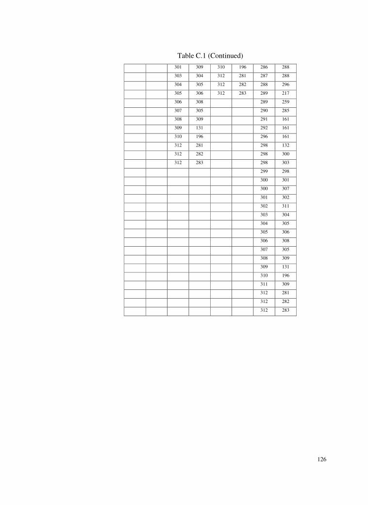
126
Table C.1 (Continued)
301 309 310 196 286 288
303 304 312 281 287 288
304 305 312 282 288 296
305 306 312 283 289 217
306 308 289 259
307 305 290 285
308 309 291 161
309 131 292 161
310 196 296 161
312 281 298 132
312 282 298 300
312 283 298 303
299 298
300 301
300 307
301 302
302 311
303 304
304 305
305 306
306 308
307 305
308 309
309 131
310 196
311 309
312 281
312 282
312 283

128
APPENDIX D
PSEUDOCODE OF THE WHOLE ALGORITHM
STEP-0: Calculate the remaining time and beginning cycle time.
STEP-1: S1=Ø, i=1, assigned=0, WC(i)=0
STEP-2: Determine and extract the tasks that can be assigned to ith station
according to the precedence relationships and zoning restrictions
among the non-assigned tasks and then put them into set S1.
STEP-3: Extract a task (k) from S1 randomly.
STEP-4: a) If C-WC(i)<t(k) then i=i+1
b) Assign task k to station i
STEP-5: assigned=assigned+1
STEP-6: If assigned<N then go to STEP-2
STEP-7: Calculate Ffirst(current);
Ffirst(current)=F1(current)+F3(current)+F5(current)
STEP-8: Best=current, Ffirst(Best)=Ffirst(current)
STEP-9: n1=0, n2=0, n3=1, worse=0, acc=0
STEP-10: temp=K1/n3
STEP-11: candidate=current
STEP-12: Choose a task (k) randomly
STEP-13: Determine the set (S2) of stations that task k can be assigned
according to the precedence relationships, zoning restrictions, station
times, cycle time and task time of task k, considering the candidate
solution.
STEP-14: Transfer the task k to a new station which is chosen from S2
randomly.
STEP-15: Adjust the station times.
STEP-16: Calculate Ffirst(candidate)
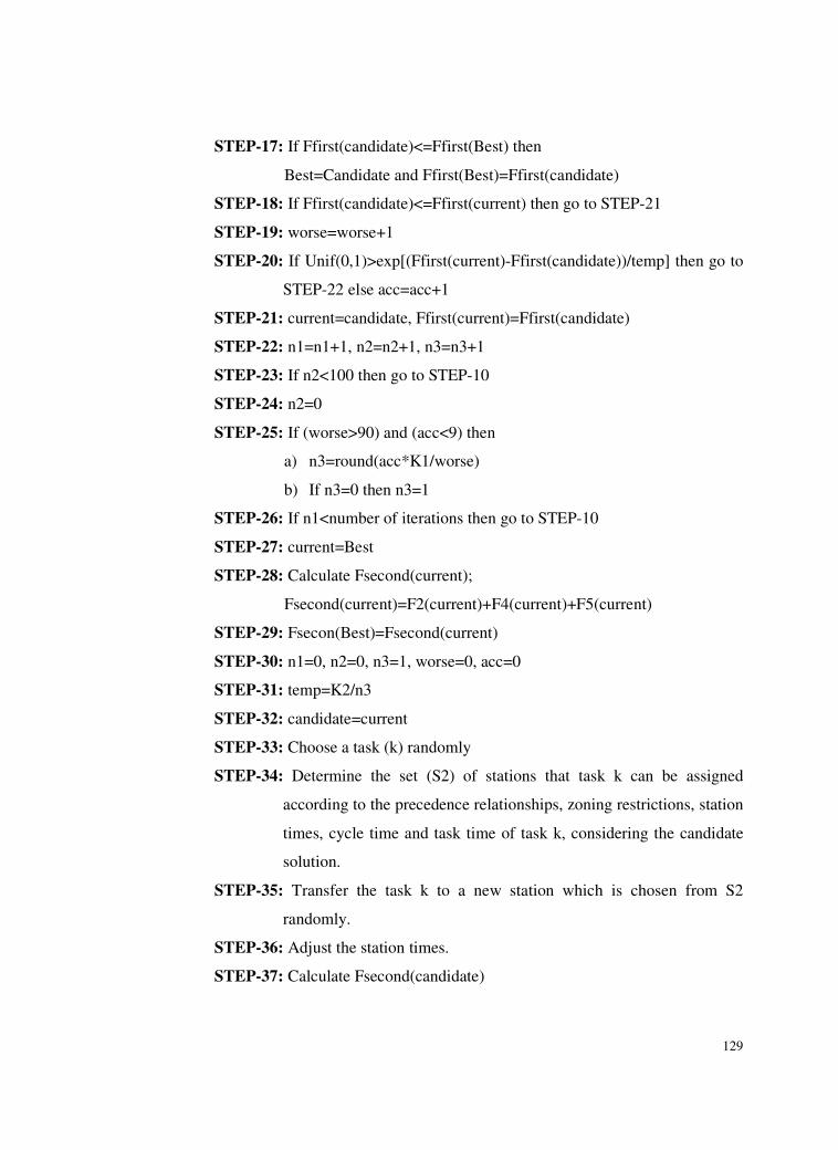
129
STEP-17: If Ffirst(candidate)<=Ffirst(Best) then
Best=Candidate and Ffirst(Best)=Ffirst(candidate)
STEP-18: If Ffirst(candidate)<=Ffirst(current) then go to STEP-21
STEP-19: worse=worse+1
STEP-20: If Unif(0,1)>exp[(Ffirst(current)-Ffirst(candidate))/temp] then go to
STEP-22 else acc=acc+1
STEP-21: current=candidate, Ffirst(current)=Ffirst(candidate)
STEP-22: n1=n1+1, n2=n2+1, n3=n3+1
STEP-23: If n2<100 then go to STEP-10
STEP-24: n2=0
STEP-25: If (worse>90) and (acc<9) then
a) n3=round(acc*K1/worse)
b) If n3=0 then n3=1
STEP-26: If n1<number of iterations then go to STEP-10
STEP-27: current=Best
STEP-28: Calculate Fsecond(current);
Fsecond(current)=F2(current)+F4(current)+F5(current)
STEP-29: Fsecon(Best)=Fsecond(current)
STEP-30: n1=0, n2=0, n3=1, worse=0, acc=0
STEP-31: temp=K2/n3
STEP-32: candidate=current
STEP-33: Choose a task (k) randomly
STEP-34: Determine the set (S2) of stations that task k can be assigned
according to the precedence relationships, zoning restrictions, station
times, cycle time and task time of task k, considering the candidate
solution.
STEP-35: Transfer the task k to a new station which is chosen from S2
randomly.
STEP-36: Adjust the station times.
STEP-37: Calculate Fsecond(candidate)
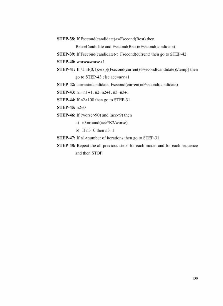
130
STEP-38: If Fsecond(candidate)<=Fsecond(Best) then
Best=Candidate and Fsecond(Best)=Fsecond(candidate)
STEP-39: If Fsecond(candidate)<=Fsecond(current) then go to STEP-42
STEP-40: worse=worse+1
STEP-41: If Unif(0,1)>exp[(Fsecond(current)-Fsecond(candidate))/temp] then
go to STEP-43 else acc=acc+1
STEP-42: current=candidate, Fsecond(current)=Fsecond(candidate)
STEP-43: n1=n1+1, n2=n2+1, n3=n3+1
STEP-44: If n2<100 then go to STEP-31
STEP-45: n2=0
STEP-46: If (worse>90) and (acc<9) then
a) n3=round(acc*K2/worse)
b) If n3=0 then n3=1
STEP-47: If n1<number of iterations then go to STEP-31
STEP-48: Repeat the all previous steps for each model and for each sequence
and then STOP.

131
APPENDIX E
RESULTS OF THE EXPERIMENTAL RUNS
Table E.1 Test problems and deviations of the found solutions from the
optimum solutions for SALBP-I
problem # of tasks # of pre.
relations C
# of stations
(optimum)
# of stations
(found) (found-opt)/opt
arcus1 83 112 3786 21 21 0
arcus1 83 112 3985 20 20 0
arcus1 83 112 4206 19 19 0
arcus1 83 112 4454 18 18 0
arcus1 83 112 4732 17 17 0
arcus1 83 112 5048 16 16 0
arcus1 83 112 5408 15 15 0
arcus1 83 112 5824 14 14 0
arcus1 83 112 5853 14 14 0
arcus1 83 112 6309 13 13 0
arcus1 83 112 6842 12 12 0
arcus1 83 112 6883 12 12 0
arcus1 83 112 7571 11 11 0
arcus1 83 112 8412 10 10 0
arcus1 83 112 8898 9 9 0
arcus1 83 112 10816 8 8 0
arcus2 111 176 5755 27 27 0
arcus2 111 176 5785 27 27 0
arcus2 111 176 6016 26 26 0
arcus2 111 176 6267 25 25 0
arcus2 111 176 6540 24 24 0
arcus2 111 176 6837 23 23 0
arcus2 111 176 7162 22 22 0
arcus2 111 176 7916 20 20 0
arcus2 111 176 8356 19 19 0
arcus2 111 176 8847 18 18 0
arcus2 111 176 9400 17 17 0
arcus2 111 176 10027 16 16 0
arcus2 111 176 10743 15 15 0
arcus2 111 176 11378 14 14 0
arcus2 111 176 11570 13 14 0.076923
arcus2 111 176 17067 9 9 0
barthold 148 173 403 14 14 0
barthold 148 173 434 13 13 0
barthold 148 173 470 12 12 0
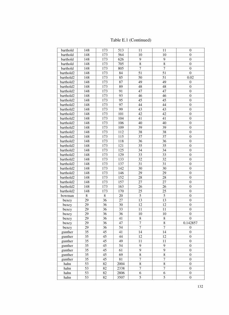
132
Table E.1 (Continued)
barthold 148 173 513 11 11 0
barthold 148 173 564 10 10 0
barthold 148 173 626 9 9 0
barthold 148 173 705 8 8 0
barthold 148 173 805 7 7 0
barthold2 148 173 84 51 51 0
barthold2 148 173 85 50 51 0.02
barthold2 148 173 87 49 49 0
barthold2 148 173 89 48 48 0
barthold2 148 173 91 47 47 0
barthold2 148 173 93 46 46 0
barthold2 148 173 95 45 45 0
barthold2 148 173 97 44 44 0
barthold2 148 173 99 43 43 0
barthold2 148 173 101 42 42 0
barthold2 148 173 104 41 41 0
barthold2 148 173 106 40 40 0
barthold2 148 173 109 39 39 0
barthold2 148 173 112 38 38 0
barthold2 148 173 115 37 37 0
barthold2 148 173 118 36 36 0
barthold2 148 173 121 35 35 0
barthold2 148 173 125 34 34 0
barthold2 148 173 129 33 33 0
barthold2 148 173 133 32 32 0
barthold2 148 173 137 31 31 0
barthold2 148 173 142 30 30 0
barthold2 148 173 146 29 29 0
barthold2 148 173 152 28 28 0
barthold2 148 173 157 27 27 0
barthold2 148 173 163 26 26 0
barthold2 148 173 170 25 25 0
bowman 8 8 20 5 5 0
buxey 29 36 27 13 13 0
buxey 29 36 30 12 12 0
buxey 29 36 33 11 11 0
buxey 29 36 36 10 10 0
buxey 29 36 41 8 8 0
buxey 29 36 47 7 8 0.142857
buxey 29 36 54 7 7 0
gunther 35 45 41 14 14 0
gunther 35 45 44 12 12 0
gunther 35 45 49 11 11 0
gunther 35 45 54 9 9 0
gunther 35 45 61 9 9 0
gunther 35 45 69 8 8 0
gunther 35 45 81 7 7 0
hahn 53 82 2004 8 8 0
hahn 53 82 2338 7 7 0
hahn 53 82 2806 6 6 0
hahn 53 82 3507 5 5 0
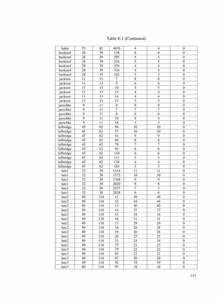
133
Table E.1 (Continued)
hahn 53 82 4676 4 4 0
heskiaof 28 39 138 8 8 0
heskiaof 28 39 205 5 5 0
heskiaof 28 39 216 5 5 0
heskiaof 28 39 256 4 4 0
heskiaof 28 39 324 4 4 0
heskiaof 28 39 342 3 3 0
jackson 11 13 7 8 8 0
jackson 11 13 9 6 6 0
jackson 11 13 10 5 5 0
jackson 11 13 13 4 4 0
jackson 11 13 14 4 4 0
jackson 11 13 21 3 3 0
jaeschke 9 11 6 8 8 0
jaeschke 9 11 7 7 7 0
jaeschke 9 11 8 6 6 0
jaeschke 9 11 10 4 4 0
jaeschke 9 11 18 3 3 0
kilbridge 45 62 56 10 10 0
kilbridge 45 62 57 10 10 0
kilbridge 45 62 62 9 9 0
kilbridge 45 62 69 8 8 0
kilbridge 45 62 79 7 7 0
kilbridge 45 62 92 6 6 0
kilbridge 45 62 110 6 6 0
kilbridge 45 62 111 5 5 0
kilbridge 45 62 138 4 4 0
kilbridge 45 62 184 3 3 0
lutz1 32 38 1414 11 11 0
lutz1 32 38 1572 10 10 0
lutz1 32 38 1768 9 9 0
lutz1 32 38 2020 8 8 0
lutz1 32 38 2357 7 7 0
lutz1 32 38 2828 6 6 0
lutz2 89 118 11 49 49 0
lutz2 89 118 12 44 44 0
lutz2 89 118 13 40 40 0
lutz2 89 118 14 37 37 0
lutz2 89 118 15 34 34 0
lutz2 89 118 16 31 31 0
lutz2 89 118 17 29 29 0
lutz2 89 118 18 28 28 0
lutz2 89 118 19 26 26 0
lutz2 89 118 20 25 25 0
lutz2 89 118 21 24 24 0
lutz3 89 118 75 23 23 0
lutz3 89 118 79 22 22 0
lutz3 89 118 83 21 21 0
lutz3 89 118 87 20 20 0
lutz3 89 118 92 19 19 0
lutz3 89 118 97 18 18 0
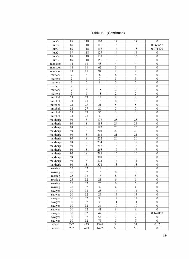
134
Table E.1 (Continued)
lutz3 89 118 103 17 17 0
lutz3 89 118 110 15 16 0.066667
lutz3 89 118 118 14 15 0.071429
lutz3 89 118 127 14 14 0
lutz3 89 118 137 13 13 0
lutz3 89 118 150 12 12 0
mansoor 11 11 48 4 4 0
mansoor 11 11 62 3 3 0
mansoor 11 11 94 2 2 0
mertens 7 6 6 6 6 0
mertens 7 6 7 5 5 0
mertens 7 6 8 5 5 0
mertens 7 6 10 3 3 0
mertens 7 6 15 2 2 0
mertens 7 6 18 2 2 0
mitchell 21 27 14 8 8 0
mitchell 21 27 15 8 8 0
mitchell 21 27 21 5 5 0
mitchell 21 27 26 5 5 0
mitchell 21 27 35 3 3 0
mitchell 21 27 39 3 3 0
mukherje 94 181 176 25 25 0
mukherje 94 181 183 24 24 0
mukherje 94 181 192 23 23 0
mukherje 94 181 201 22 22 0
mukherje 94 181 211 21 21 0
mukherje 94 181 222 20 20 0
mukherje 94 181 234 19 19 0
mukherje 94 181 248 18 18 0
mukherje 94 181 263 17 17 0
mukherje 94 181 281 16 16 0
mukherje 94 181 301 15 15 0
mukherje 94 181 324 14 14 0
mukherje 94 181 351 13 13 0
roszieg 25 32 14 10 10 0
roszieg 25 32 16 8 8 0
roszieg 25 32 18 8 8 0
roszieg 25 32 21 6 6 0
roszieg 25 32 25 6 6 0
roszieg 25 32 32 4 4 0
sawyer 30 32 25 14 14 0
sawyer 30 32 27 13 13 0
sawyer 30 32 30 12 12 0
sawyer 30 32 33 11 11 0
sawyer 30 32 36 10 10 0
sawyer 30 32 41 8 8 0
sawyer 30 32 47 7 8 0.142857
sawyer 30 32 54 7 7 0
sawyer 30 32 75 5 5 0
scholl 297 423 1394 50 51 0.02
scholl 297 423 1422 50 50 0

135
Table E.1 (Continued)
scholl 297 423 1452 48 49 0.020833
scholl 297 423 1515 46 47 0.021739
scholl 297 423 1548 46 46 0
scholl 297 423 1584 44 45 0.022727
scholl 297 423 1620 44 44 0
scholl 297 423 1659 42 43 0.02381
scholl 297 423 1742 40 41 0.025
scholl 297 423 1787 39 40 0.025641
scholl 297 423 1834 38 39 0.026316
scholl 297 423 1883 37 38 0.027027
scholl 297 423 1935 36 37 0.027778
scholl 297 423 1991 35 36 0.028571
scholl 297 423 2049 34 35 0.029412
scholl 297 423 2111 33 34 0.030303
scholl 297 423 2177 32 33 0.03125
scholl 297 423 2247 31 32 0.032258
scholl 297 423 2322 30 31 0.033333
scholl 297 423 2402 29 30 0.034483
scholl 297 423 2488 28 29 0.035714
scholl 297 423 2580 27 28 0.037037
scholl 297 423 2680 26 27 0.038462
scholl 297 423 2787 25 26 0.04
tonge 70 86 160 23 23 0
tonge 70 86 168 22 22 0
tonge 70 86 176 21 21 0
tonge 70 86 185 20 20 0
tonge 70 86 195 19 19 0
tonge 70 86 207 18 18 0
tonge 70 86 220 17 17 0
tonge 70 86 234 16 16 0
tonge 70 86 251 14 15 0.071429
tonge 70 86 270 14 14 0
tonge 70 86 293 13 13 0
tonge 70 86 320 11 11 0
tonge 70 86 364 10 10 0
tonge 70 86 410 9 9 0
tonge 70 86 468 8 8 0
tonge 70 86 527 7 7 0
warnecke 58 70 54 31 31 0
warnecke 58 70 56 29 29 0
warnecke 58 70 58 29 29 0
warnecke 58 70 60 27 27 0
warnecke 58 70 62 27 27 0
warnecke 58 70 65 25 25 0
warnecke 58 70 68 24 24 0
warnecke 58 70 71 23 23 0
warnecke 58 70 74 22 22 0
warnecke 58 70 78 21 21 0
warnecke 58 70 82 20 20 0
warnecke 58 70 86 19 19 0
warnecke 58 70 92 17 17 0

136
Table E.1 (Continued)
warnecke 58 70 97 17 17 0
warnecke 58 70 104 15 15 0
warnecke 58 70 111 14 14 0
wee-mag 75 87 28 63 63 0
wee-mag 75 87 29 63 63 0
wee-mag 75 87 30 62 62 0
wee-mag 75 87 31 62 62 0
wee-mag 75 87 32 61 61 0
wee-mag 75 87 33 61 61 0
wee-mag 75 87 34 61 61 0
wee-mag 75 87 35 60 60 0
wee-mag 75 87 36 60 60 0
wee-mag 75 87 37 60 60 0
wee-mag 75 87 38 60 60 0
wee-mag 75 87 39 60 60 0
wee-mag 75 87 40 60 60 0
wee-mag 75 87 41 59 59 0
wee-mag 75 87 42 55 55 0
wee-mag 75 87 43 50 50 0
wee-mag 75 87 45 38 38 0
wee-mag 75 87 46 34 34 0
wee-mag 75 87 49 32 32 0
wee-mag 75 87 50 32 32 0
wee-mag 75 87 52 31 31 0
wee-mag 75 87 54 31 31 0
wee-mag 75 87 56 30 30 0

137
Table E.2 Descriptive statistics of deviations for SALBP-I
problem average of
deviations
std.dev. of
deviations min. deviation max. deviation
arcus1 0 0 0 0
arcus2 0.00480769 0.0192308 0 0.0769231
barthold 0 0 0 0
barthold2 0.00074074 0.003849 0 0.02
bowman 0 0 0 0
buxey 0.02040816 0.0539949 0 0.1428571
gunther 0 0 0 0
hahn 0 0 0 0
heskiaof 0 0 0 0
jackson 0 0 0 0
jaeschke 0 0 0 0
kilbridge 0 0 0 0
lutz1 0 0 0 0
lutz2 0 0 0 0
lutz3 0.01150794 0.0268959 0 0.0714286
mansoor 0 0 0 0
mertens 0 0 0 0
mitchell 0 0 0 0
mukherje 0 0 0 0
roszieg 0 0 0 0
sawyer 0.01587302 0.047619 0 0.1428571
scholl 0.02548726 0.0112679 0 0.04
tonge 0.00446429 0.0178571 0 0.0714286
warnecke 0 0 0 0
wee-mag 0 0 0 0
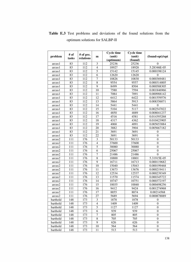
138
Table E.3 Test problems and deviations of the found solutions from the
optimum solutions for SALBP-II
problem # of
tasks
# of pre.
relations m
Cycle time
(unit)
(optimum)
Cycle time
(unit)
(found)
(found-opt)/opt
arcus1 83 112 3 25236 25236 0
arcus1 83 112 4 18927 18928 5.28346E-05
arcus1 83 112 5 15142 15145 0.000198124
arcus1 83 112 6 12620 12620 0
arcus1 83 112 7 10826 10830 0.000369481
arcus1 83 112 8 9554 9557 0.000314005
arcus1 83 112 9 8499 8504 0.000588305
arcus1 83 112 10 7580 7594 0.001846966
arcus1 83 112 11 7084 7091 0.000988142
arcus1 83 112 12 6412 6422 0.001559576
arcus1 83 112 13 5864 5913 0.008356071
arcus1 83 112 14 5441 5441 0
arcus1 83 112 15 5104 5117 0.002547022
arcus1 83 112 16 4850 4889 0.008041237
arcus1 83 112 17 4516 4581 0.014393268
arcus1 83 112 18 4317 4362 0.010423905
arcus1 83 112 19 4068 4091 0.005653884
arcus1 83 112 20 3882 3904 0.005667182
arcus1 83 112 21 3691 3691 0
arcus1 83 112 22 3691 3691 0
arcus2 111 176 3 50133 50133 0
arcus2 111 176 4 37600 37600 0
arcus2 111 176 5 30080 30080 0
arcus2 111 176 6 25067 25067 0
arcus2 111 176 7 21486 21486 0
arcus2 111 176 8 18800 18801 5.31915E-05
arcus2 111 176 9 16711 16713 0.000119682
arcus2 111 176 10 15040 15043 0.000199468
arcus2 111 176 11 13673 13676 0.000219411
arcus2 111 176 12 12534 12537 0.000239349
arcus2 111 176 13 11570 11574 0.000345722
arcus2 111 176 14 10747 10751 0.000372197
arcus2 111 176 15 10035 10040 0.000498256
arcus2 111 176 16 9412 9424 0.001274968
arcus2 111 176 17 8855 8874 0.00214568
arcus2 111 176 27 5689 5694 0.000878889
barthold 148 173 3 1878 1878 0
barthold 148 173 4 1409 1409 0
barthold 148 173 5 1127 1127 0
barthold 148 173 6 939 939 0
barthold 148 173 7 805 805 0
barthold 148 173 8 705 705 0
barthold 148 173 9 626 626 0
barthold 148 173 10 564 564 0
barthold 148 173 11 513 513 0

139
Table E.3 (Continued)
barthold 148 173 12 470 470 0
barthold 148 173 13 434 434 0
barthold 148 173 14 403 403 0
barthold 148 173 15 383 383 0
barthold2 148 173 27 157 157 0
barthold2 148 173 28 152 152 0
barthold2 148 173 29 146 146 0
barthold2 148 173 30 142 142 0
barthold2 148 173 31 137 137 0
barthold2 148 173 32 133 133 0
barthold2 148 173 33 129 129 0
barthold2 148 173 34 125 125 0
barthold2 148 173 35 121 121 0
barthold2 148 173 36 118 118 0
barthold2 148 173 37 115 115 0
barthold2 148 173 38 112 112 0
barthold2 148 173 39 109 109 0
barthold2 148 173 40 106 106 0
barthold2 148 173 41 104 104 0
barthold2 148 173 42 101 101 0
barthold2 148 173 43 99 99 0
barthold2 148 173 44 97 97 0
barthold2 148 173 45 95 95 0
barthold2 148 173 46 93 93 0
barthold2 148 173 47 91 91 0
barthold2 148 173 48 89 89 0
barthold2 148 173 49 87 87 0
barthold2 148 173 50 85 86 0.011764706
barthold2 148 173 51 84 84 0
buxey 29 36 7 47 48 0.021276596
buxey 29 36 8 41 41 0
buxey 29 36 9 37 37 0
buxey 29 36 10 34 34 0
buxey 29 36 11 32 32 0
buxey 29 36 12 28 28 0
buxey 29 36 13 27 27 0
buxey 29 36 14 25 25 0
gunther 35 45 6 84 84 0
gunther 35 45 7 72 72 0
gunther 35 45 8 63 63 0
gunther 35 45 9 54 54 0
gunther 35 45 10 50 50 0
gunther 35 45 11 48 48 0
gunther 35 45 12 44 44 0
gunther 35 45 13 42 42 0
gunther 35 45 14 40 40 0
gunther 35 45 15 40 40 0
hahn 53 82 3 4787 4787 0
hahn 53 82 4 3677 3677 0
hahn 53 82 5 2823 2823 0
hahn 53 82 6 2400 2400 0
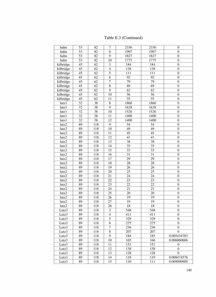
140
Table E.3 (Continued)
hahn 53 82 7 2336 2336 0
hahn 53 82 8 1907 1907 0
hahn 53 82 9 1827 1827 0
hahn 53 82 10 1775 1775 0
kilbridge 45 62 3 184 184 0
kilbridge 45 62 4 138 138 0
kilbridge 45 62 5 111 111 0
kilbridge 45 62 6 92 92 0
kilbridge 45 62 7 79 79 0
kilbridge 45 62 8 69 69 0
kilbridge 45 62 9 62 62 0
kilbridge 45 62 10 56 56 0
kilbridge 45 62 11 55 55 0
lutz1 32 38 8 1860 1860 0
lutz1 32 38 9 1638 1638 0
lutz1 32 38 10 1526 1526 0
lutz1 32 38 11 1400 1400 0
lutz1 32 38 12 1400 1400 0
lutz2 89 118 9 54 54 0
lutz2 89 118 10 49 49 0
lutz2 89 118 11 45 45 0
lutz2 89 118 12 41 41 0
lutz2 89 118 13 38 38 0
lutz2 89 118 14 35 35 0
lutz2 89 118 15 33 33 0
lutz2 89 118 16 31 31 0
lutz2 89 118 17 29 29 0
lutz2 89 118 18 28 28 0
lutz2 89 118 19 26 26 0
lutz2 89 118 20 25 25 0
lutz2 89 118 21 24 24 0
lutz2 89 118 22 23 23 0
lutz2 89 118 23 22 22 0
lutz2 89 118 24 21 21 0
lutz2 89 118 25 20 20 0
lutz2 89 118 26 19 19 0
lutz2 89 118 27 19 19 0
lutz2 89 118 28 18 18 0
Lutz3 89 118 3 548 548 0
Lutz3 89 118 4 411 411 0
Lutz3 89 118 5 329 329 0
Lutz3 89 118 6 275 275 0
Lutz3 89 118 7 236 236 0
Lutz3 89 118 8 207 207 0
Lutz3 89 118 9 184 185 0.005434783
Lutz3 89 118 10 165 166 0.006060606
Lutz3 89 118 11 151 151 0
Lutz3 89 118 12 138 138 0
Lutz3 89 118 13 128 128 0
Lutz3 89 118 14 118 119 0.008474576
Lutz3 89 118 15 110 111 0.009090909

141
Table E.3 (Continued)
Lutz3 89 118 16 105 105 0
Lutz3 89 118 17 98 98 0
Lutz3 89 118 18 93 93 0
Lutz3 89 118 19 89 89 0
Lutz3 89 118 20 85 85 0
Lutz3 89 118 21 80 80 0
Lutz3 89 118 22 76 77 0.013157895
Lutz3 89 118 23 74 74 0
mukherje 94 181 3 1403 1403 0
mukherje 94 181 4 1052 1052 0
mukherje 94 181 5 844 844 0
mukherje 94 181 6 704 704 0
mukherje 94 181 7 621 621 0
mukherje 94 181 8 532 532 0
mukherje 94 181 9 471 471 0
mukherje 94 181 10 424 424 0
mukherje 94 181 11 391 391 0
mukherje 94 181 12 358 358 0
mukherje 94 181 13 325 326 0.003076923
mukherje 94 181 14 311 311 0
mukherje 94 181 15 288 288 0
mukherje 94 181 16 268 270 0.007462687
mukherje 94 181 17 251 251 0
mukherje 94 181 18 239 239 0
mukherje 94 181 19 226 226 0
mukherje 94 181 20 220 221 0.004545455
mukherje 94 181 21 208 208 0
mukherje 94 181 22 200 200 0
mukherje 94 181 23 189 189 0
mukherje 94 181 24 179 179 0
mukherje 94 181 25 172 172 0
mukherje 94 181 26 171 171 0
sawyer 30 32 7 47 48 0.021276596
sawyer 30 32 8 41 41 0
sawyer 30 32 9 37 37 0
sawyer 30 32 10 34 34 0
sawyer 30 32 11 31 31 0
sawyer 30 32 12 28 28 0
sawyer 30 32 13 26 26 0
sawyer 30 32 14 25 25 0
scholl 297 423 25 2787 2796 0.003229279
scholl 297 423 26 2680 2687 0.00261194
scholl 297 423 27 2580 2587 0.002713178
scholl 297 423 28 2488 2496 0.003215434
scholl 297 423 29 2402 2408 0.002497918
scholl 297 423 30 2322 2330 0.003445306
scholl 297 423 31 2247 2257 0.004450378
scholl 297 423 32 2177 2195 0.008268259
scholl 297 423 33 2111 2127 0.007579346
scholl 297 423 34 2049 2068 0.009272816
scholl 297 423 35 1991 2007 0.008036163
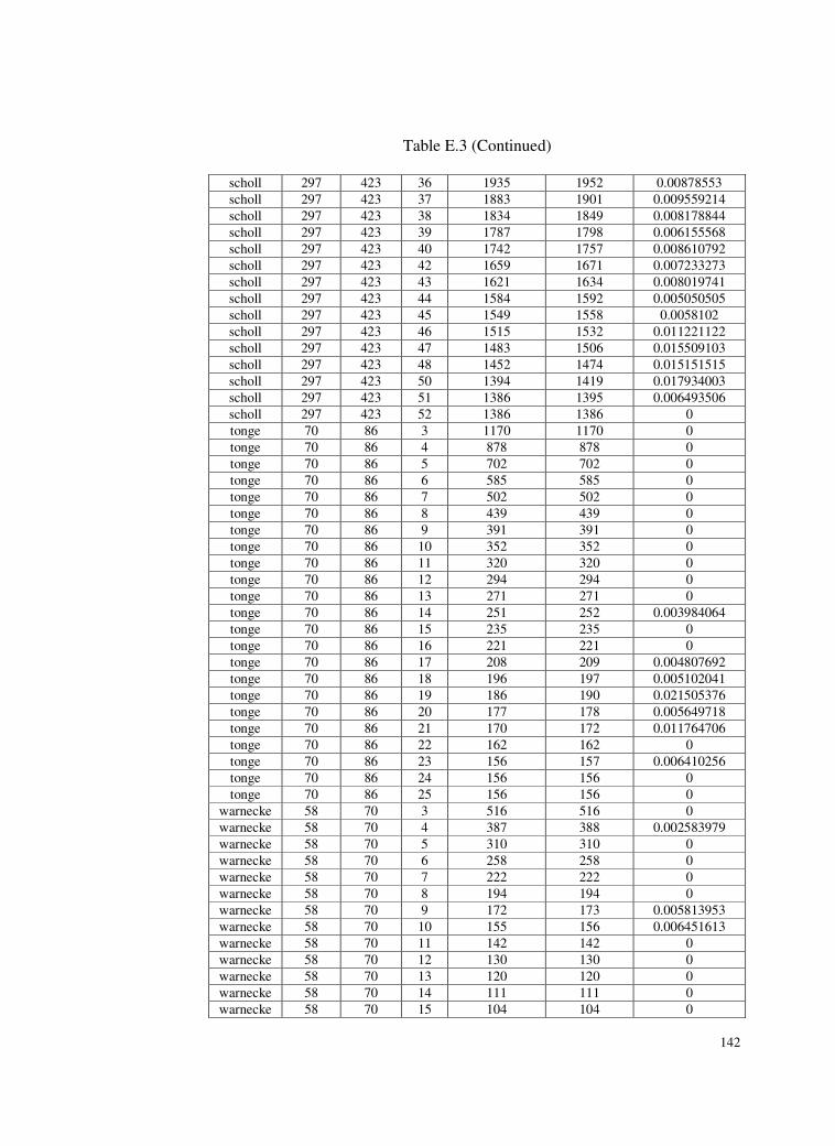
142
Table E.3 (Continued)
scholl 297 423 36 1935 1952 0.00878553
scholl 297 423 37 1883 1901 0.009559214
scholl 297 423 38 1834 1849 0.008178844
scholl 297 423 39 1787 1798 0.006155568
scholl 297 423 40 1742 1757 0.008610792
scholl 297 423 42 1659 1671 0.007233273
scholl 297 423 43 1621 1634 0.008019741
scholl 297 423 44 1584 1592 0.005050505
scholl 297 423 45 1549 1558 0.0058102
scholl 297 423 46 1515 1532 0.011221122
scholl 297 423 47 1483 1506 0.015509103
scholl 297 423 48 1452 1474 0.015151515
scholl 297 423 50 1394 1419 0.017934003
scholl 297 423 51 1386 1395 0.006493506
scholl 297 423 52 1386 1386 0
tonge 70 86 3 1170 1170 0
tonge 70 86 4 878 878 0
tonge 70 86 5 702 702 0
tonge 70 86 6 585 585 0
tonge 70 86 7 502 502 0
tonge 70 86 8 439 439 0
tonge 70 86 9 391 391 0
tonge 70 86 10 352 352 0
tonge 70 86 11 320 320 0
tonge 70 86 12 294 294 0
tonge 70 86 13 271 271 0
tonge 70 86 14 251 252 0.003984064
tonge 70 86 15 235 235 0
tonge 70 86 16 221 221 0
tonge 70 86 17 208 209 0.004807692
tonge 70 86 18 196 197 0.005102041
tonge 70 86 19 186 190 0.021505376
tonge 70 86 20 177 178 0.005649718
tonge 70 86 21 170 172 0.011764706
tonge 70 86 22 162 162 0
tonge 70 86 23 156 157 0.006410256
tonge 70 86 24 156 156 0
tonge 70 86 25 156 156 0
warnecke 58 70 3 516 516 0
warnecke 58 70 4 387 388 0.002583979
warnecke 58 70 5 310 310 0
warnecke 58 70 6 258 258 0
warnecke 58 70 7 222 222 0
warnecke 58 70 8 194 194 0
warnecke 58 70 9 172 173 0.005813953
warnecke 58 70 10 155 156 0.006451613
warnecke 58 70 11 142 142 0
warnecke 58 70 12 130 130 0
warnecke 58 70 13 120 120 0
warnecke 58 70 14 111 111 0
warnecke 58 70 15 104 104 0
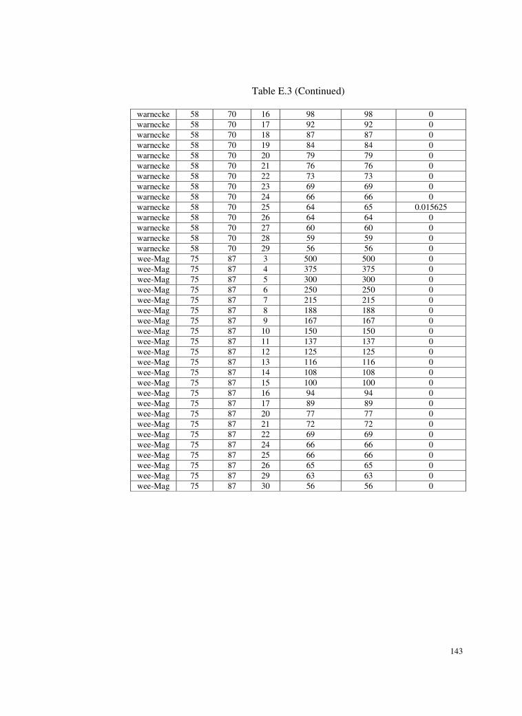
143
Table E.3 (Continued)
warnecke 58 70 16 98 98 0
warnecke 58 70 17 92 92 0
warnecke 58 70 18 87 87 0
warnecke 58 70 19 84 84 0
warnecke 58 70 20 79 79 0
warnecke 58 70 21 76 76 0
warnecke 58 70 22 73 73 0
warnecke 58 70 23 69 69 0
warnecke 58 70 24 66 66 0
warnecke 58 70 25 64 65 0.015625
warnecke 58 70 26 64 64 0
warnecke 58 70 27 60 60 0
warnecke 58 70 28 59 59 0
warnecke 58 70 29 56 56 0
wee-Mag 75 87 3 500 500 0
wee-Mag 75 87 4 375 375 0
wee-Mag 75 87 5 300 300 0
wee-Mag 75 87 6 250 250 0
wee-Mag 75 87 7 215 215 0
wee-Mag 75 87 8 188 188 0
wee-Mag 75 87 9 167 167 0
wee-Mag 75 87 10 150 150 0
wee-Mag 75 87 11 137 137 0
wee-Mag 75 87 12 125 125 0
wee-Mag 75 87 13 116 116 0
wee-Mag 75 87 14 108 108 0
wee-Mag 75 87 15 100 100 0
wee-Mag 75 87 16 94 94 0
wee-Mag 75 87 17 89 89 0
wee-Mag 75 87 20 77 77 0
wee-Mag 75 87 21 72 72 0
wee-Mag 75 87 22 69 69 0
wee-Mag 75 87 24 66 66 0
wee-Mag 75 87 25 66 66 0
wee-Mag 75 87 26 65 65 0
wee-Mag 75 87 29 63 63 0
wee-Mag 75 87 30 56 56 0

144
Table E.4 Descriptive statistics of deviations for SALBP-II
problem average of
deviations
std.dev. of
deviations Min. deviation Max. deviation
arcus1 0.00305 0.004244 0 0.014393
arcus2 0.000397 0.000586 0 0.002146
barthold 0 0 0 0
barthold2 0.000471 0.002353 0 0.011765
Buxey 0.00266 0.007522 0 0.021277
gunther 0 0 0 0
hahn 0 0 0 0
kilbridge 0 0 0 0
lutz1 0 0 0 0
lutz2 0 0 0 0
lutz3 0.00201 0.003931 0 0.013158
mukherje 0.000629 0.001822 0 0.007463
sawyer 0.00266 0.007522 0 0.021277
scholl 0.00727 0.004281 0 0.017934
tonge 0.002575 0.005163 0 0.021505
warnecke 0.001129 0.00335 0 0.015625
wee-mag 0 0 0 0
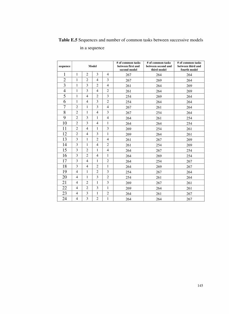
145
Table E.5 Sequences and number of common tasks between successive models
in a sequence
sequence Model
# of common tasks
between first and
second model
# of common tasks
between second and
third model
# of common tasks
between third and
fourth model
1 1 2 3 4 267 264 264
2 1 2 4 3 267 269 264
3 1 3 2 4 261 264 269
4 1 3 4 2 261 264 269
5 1 4 2 3 254 269 264
6 1 4 3 2 254 264 264
7 2 1 3 4 267 261 264
8 2 1 4 3 267 254 264
9 2 3 1 4 264 261 254
10 2 3 4 1 264 264 254
11 2 4 1 3 269 254 261
12 2 4 3 1 269 264 261
13 3 1 2 4 261 267 269
14 3 1 4 2 261 254 269
15 3 2 1 4 264 267 254
16 3 2 4 1 264 269 254
17 3 4 1 2 264 254 267
18 3 4 2 1 264 269 267
19 4 1 2 3 254 267 264
20 4 1 3 2 254 261 264
21 4 2 1 3 269 267 261
22 4 2 3 1 269 264 261
23 4 3 1 2 264 261 267
24 4 3 2 1 264 264 267
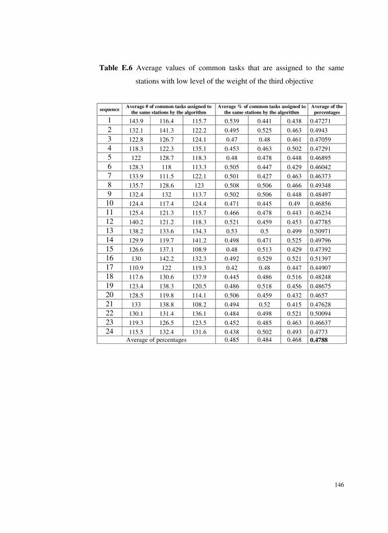
146
Table E.6 Average values of common tasks that are assigned to the same
stations with low level of the weight of the third objective
sequence Average # of common tasks assigned to
the same stations by the algorithm
Average % of common tasks assigned to
the same stations by the algorithm
Average of the
percentages
1 143.9 116.4 115.7 0.539 0.441 0.438 0.47271
2 132.1 141.3 122.2 0.495 0.525 0.463 0.4943
3 122.8 126.7 124.1 0.47 0.48 0.461 0.47059
4 118.3 122.3 135.1 0.453 0.463 0.502 0.47291
5 122 128.7 118.3 0.48 0.478 0.448 0.46895
6 128.3 118 113.3 0.505 0.447 0.429 0.46042
7 133.9 111.5 122.1 0.501 0.427 0.463 0.46373
8 135.7 128.6 123 0.508 0.506 0.466 0.49348
9 132.4 132 113.7 0.502 0.506 0.448 0.48497
10 124.4 117.4 124.4 0.471 0.445 0.49 0.46856
11 125.4 121.3 115.7 0.466 0.478 0.443 0.46234
12 140.2 121.2 118.3 0.521 0.459 0.453 0.47785
13 138.2 133.6 134.3 0.53 0.5 0.499 0.50971
14 129.9 119.7 141.2 0.498 0.471 0.525 0.49796
15 126.6 137.1 108.9 0.48 0.513 0.429 0.47392
16 130 142.2 132.3 0.492 0.529 0.521 0.51397
17 110.9 122 119.3 0.42 0.48 0.447 0.44907
18 117.6 130.6 137.9 0.445 0.486 0.516 0.48248
19 123.4 138.3 120.5 0.486 0.518 0.456 0.48675
20 128.5 119.8 114.1 0.506 0.459 0.432 0.4657
21 133 138.8 108.2 0.494 0.52 0.415 0.47628
22 130.1 131.4 136.1 0.484 0.498 0.521 0.50094
23 119.3 126.5 123.5 0.452 0.485 0.463 0.46637
24 115.5 132.4 131.6 0.438 0.502 0.493 0.4773
Average of percentages 0.485 0.484 0.468 0.4788

147
Table E.7 Average values of common tasks that are assigned to the same
stations with intermediate level of the weight of the third objective
sequence Average # of common tasks assigned to
the same stations by the algorithm
Average % of common tasks assigned to
the same stations by the algorithm
Average of the
percentages
1 243.2 238.4 230 0.911 0.903 0.871 0.89503
2 240.4 229.2 240.4 0.9 0.852 0.911 0.88768
3 230 236.8 236.4 0.881 0.897 0.879 0.88567
4 233.8 235 242.7 0.896 0.89 0.902 0.89606
5 218 242.8 241.8 0.858 0.903 0.916 0.89226
6 206 235.4 242 0.811 0.892 0.917 0.87312
7 252.2 234.2 230 0.945 0.897 0.871 0.90437
8 249.4 218.8 242.4 0.934 0.861 0.918 0.90456
9 237 241.6 209.2 0.898 0.926 0.824 0.88234
10 237.8 230.4 227.2 0.901 0.873 0.894 0.88932
11 230.1 226.6 231.6 0.855 0.892 0.887 0.87829
12 230.4 236.8 238.2 0.857 0.897 0.913 0.88871
13 233.4 244 238.6 0.894 0.914 0.887 0.89837
14 237.2 216.8 243 0.909 0.854 0.903 0.88857
15 229 248 224.4 0.867 0.929 0.883 0.89324
16 228.6 223.4 224 0.866 0.83 0.882 0.85943
17 216.6 221.6 249.6 0.82 0.872 0.935 0.87591
18 215.4 239.1 253 0.816 0.889 0.948 0.88411
19 205.2 249.2 242.2 0.808 0.933 0.917 0.88621
20 205.2 235.8 240.8 0.808 0.903 0.912 0.87448
21 218.3 251.6 236 0.812 0.942 0.904 0.88602
22 218.1 241.6 242.6 0.811 0.915 0.93 0.88514
23 213.4 234 244.2 0.808 0.897 0.915 0.87316
24 217 222 251.2 0.822 0.841 0.941 0.8679
Average of percentages 0.862 0.892 0.902 0.88541
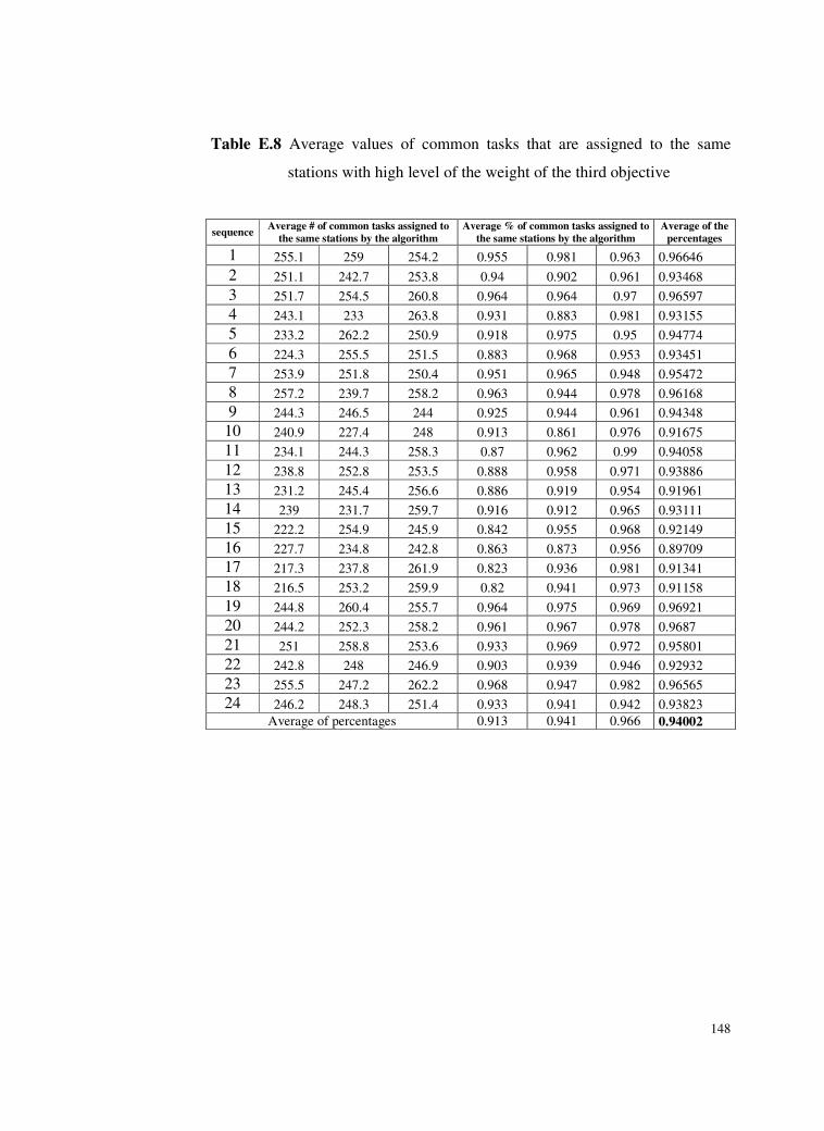
148
Table E.8 Average values of common tasks that are assigned to the same
stations with high level of the weight of the third objective
sequence Average # of common tasks assigned to
the same stations by the algorithm
Average % of common tasks assigned to
the same stations by the algorithm
Average of the
percentages
1 255.1 259 254.2 0.955 0.981 0.963 0.96646
2 251.1 242.7 253.8 0.94 0.902 0.961 0.93468
3 251.7 254.5 260.8 0.964 0.964 0.97 0.96597
4 243.1 233 263.8 0.931 0.883 0.981 0.93155
5 233.2 262.2 250.9 0.918 0.975 0.95 0.94774
6 224.3 255.5 251.5 0.883 0.968 0.953 0.93451
7 253.9 251.8 250.4 0.951 0.965 0.948 0.95472
8 257.2 239.7 258.2 0.963 0.944 0.978 0.96168
9 244.3 246.5 244 0.925 0.944 0.961 0.94348
10 240.9 227.4 248 0.913 0.861 0.976 0.91675
11 234.1 244.3 258.3 0.87 0.962 0.99 0.94058
12 238.8 252.8 253.5 0.888 0.958 0.971 0.93886
13 231.2 245.4 256.6 0.886 0.919 0.954 0.91961
14 239 231.7 259.7 0.916 0.912 0.965 0.93111
15 222.2 254.9 245.9 0.842 0.955 0.968 0.92149
16 227.7 234.8 242.8 0.863 0.873 0.956 0.89709
17 217.3 237.8 261.9 0.823 0.936 0.981 0.91341
18 216.5 253.2 259.9 0.82 0.941 0.973 0.91158
19 244.8 260.4 255.7 0.964 0.975 0.969 0.96921
20 244.2 252.3 258.2 0.961 0.967 0.978 0.9687
21 251 258.8 253.6 0.933 0.969 0.972 0.95801
22 242.8 248 246.9 0.903 0.939 0.946 0.92932
23 255.5 247.2 262.2 0.968 0.947 0.982 0.96565
24 246.2 248.3 251.4 0.933 0.941 0.942 0.93823
Average of percentages 0.913 0.941 0.966 0.94002

149
Table E.9 Average values of TSTs at the beginning of the runs with low level
of the weight of the third objective
Sequence
Average
Values of
TST
Average
Values of
TST
Average
Values of
TST
Average
Values of
TST
1 256.2 300.8 317.4 315.47
2 256.2 333.78 305.69 327.74
3 256.2 294.4 319.72 356.2
4 256.2 299.2 319.7 330.43
5 256.2 293.57 306.65 318.31
6 256.2 289.7 296.94 331.9
7 242 265.16 366.44 307.83
8 242 263.2 309.94 369.02
9 242 289.83 270.48 375.93
10 242 270.71 267.71 273
11 242 284.14 265.16 315.31
12 242 268.32 294.3 268.8
13 282 260.96 330.19 341.02
14 287.04 262.36 319.5 338.03
15 287.04 246.64 268.52 358.63
16 287.04 245.77 266.71 271.04
17 276.96 270.54 261.52 361.08
18 292.08 281.91 247.22 268.8
19 281.84 256.2 320.42 321.52
20 276.8 257.88 286.55 329.82
21 266.72 242.87 267.12 282.94
22 266.72 243.45 281.98 272.16
23 266.72 282.57 259.84 343.63
24 281.84 282.87 248.38 267.96
Avg. of the columns 264.25 274.4513 291.5867 318.6071
StdD. of the columns 17.3995 21.98391 30.27326 34.967 Avg. of the values of
Model1 in the column 256.2 260.96 265.44 270.2933
StdD. of the values of
Model1 in the column 0 3.36932 4.111331 2.062646
Avg. of the values of
Model2 in the column 242 268.885 295.43 339.1483
StdD. of the values of
Model2 in the column 0 38.94301 37.6472 11.98248
Avg. of the values of
Model3 in the column 285.36 286.5967 307.2683 322.4733
StdD. of the values of
Model3 in the column 5.20529 10.12599 31.45644 27.66503
Avg. of the values of
Model4 in the column 273.44 281.3633 298.2083 342.5133
StdD. of the values of Model4 in the column
7.587948 10.13691 24.62165 26.45846
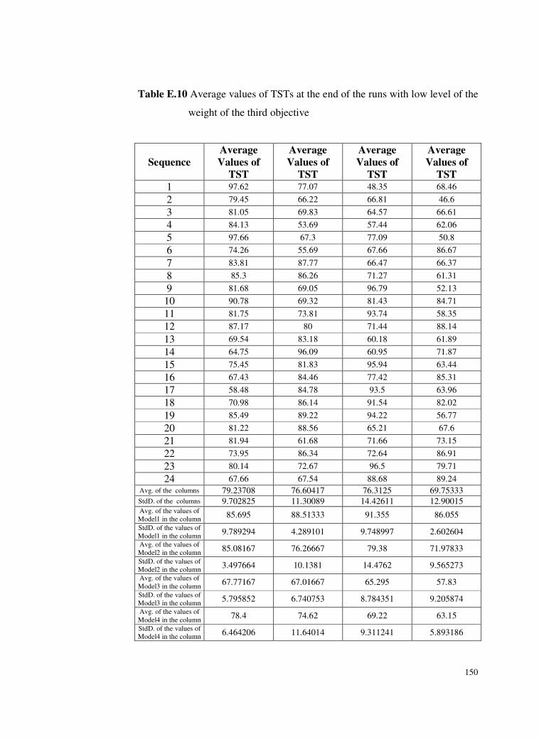
150
Table E.10 Average values of TSTs at the end of the runs with low level of the
weight of the third objective
Sequence
Average
Values of
TST
Average
Values of
TST
Average
Values of
TST
Average
Values of
TST
1 97.62 77.07 48.35 68.46
2 79.45 66.22 66.81 46.6
3 81.05 69.83 64.57 66.61
4 84.13 53.69 57.44 62.06
5 97.66 67.3 77.09 50.8
6 74.26 55.69 67.66 86.67
7 83.81 87.77 66.47 66.37
8 85.3 86.26 71.27 61.31
9 81.68 69.05 96.79 52.13
10 90.78 69.32 81.43 84.71
11 81.75 73.81 93.74 58.35
12 87.17 80 71.44 88.14
13 69.54 83.18 60.18 61.89
14 64.75 96.09 60.95 71.87
15 75.45 81.83 95.94 63.44
16 67.43 84.46 77.42 85.31
17 58.48 84.78 93.5 63.96
18 70.98 86.14 91.54 82.02
19 85.49 89.22 94.22 56.77
20 81.22 88.56 65.21 67.6
21 81.94 61.68 71.66 73.15
22 73.95 86.34 72.64 86.91
23 80.14 72.67 96.5 79.71
24 67.66 67.54 88.68 89.24
Avg. of the columns 79.23708 76.60417 76.3125 69.75333
StdD. of the columns 9.702825 11.30089 14.42611 12.90015 Avg. of the values of
Model1 in the column 85.695 88.51333 91.355 86.055
StdD. of the values of
Model1 in the column 9.789294 4.289101 9.748997 2.602604
Avg. of the values of
Model2 in the column 85.08167 76.26667 79.38 71.97833
StdD. of the values of
Model2 in the column 3.497664 10.1381 14.4762 9.565273
Avg. of the values of
Model3 in the column 67.77167 67.01667 65.295 57.83
StdD. of the values of
Model3 in the column 5.795852 6.740753 8.784351 9.205874
Avg. of the values of
Model4 in the column 78.4 74.62 69.22 63.15
StdD. of the values of Model4 in the column
6.464206 11.64014 9.311241 5.893186
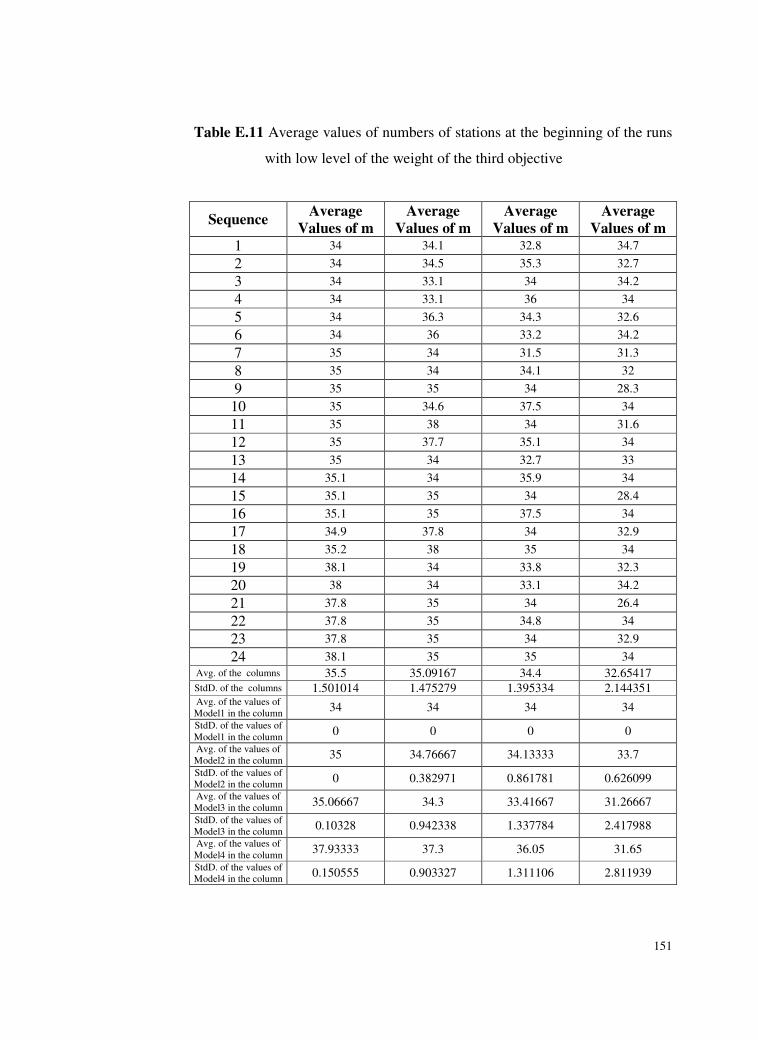
151
Table E.11 Average values of numbers of stations at the beginning of the runs
with low level of the weight of the third objective
Sequence Average
Values of m
Average
Values of m
Average
Values of m
Average
Values of m
1 34 34.1 32.8 34.7
2 34 34.5 35.3 32.7
3 34 33.1 34 34.2
4 34 33.1 36 34
5 34 36.3 34.3 32.6
6 34 36 33.2 34.2
7 35 34 31.5 31.3
8 35 34 34.1 32
9 35 35 34 28.3
10 35 34.6 37.5 34
11 35 38 34 31.6
12 35 37.7 35.1 34
13 35 34 32.7 33
14 35.1 34 35.9 34
15 35.1 35 34 28.4
16 35.1 35 37.5 34
17 34.9 37.8 34 32.9
18 35.2 38 35 34
19 38.1 34 33.8 32.3
20 38 34 33.1 34.2
21 37.8 35 34 26.4
22 37.8 35 34.8 34
23 37.8 35 34 32.9
24 38.1 35 35 34
Avg. of the columns 35.5 35.09167 34.4 32.65417
StdD. of the columns 1.501014 1.475279 1.395334 2.144351 Avg. of the values of
Model1 in the column 34 34 34 34
StdD. of the values of
Model1 in the column 0 0 0 0
Avg. of the values of
Model2 in the column 35 34.76667 34.13333 33.7
StdD. of the values of
Model2 in the column 0 0.382971 0.861781 0.626099
Avg. of the values of
Model3 in the column 35.06667 34.3 33.41667 31.26667
StdD. of the values of
Model3 in the column 0.10328 0.942338 1.337784 2.417988
Avg. of the values of
Model4 in the column 37.93333 37.3 36.05 31.65
StdD. of the values of
Model4 in the column 0.150555 0.903327 1.311106 2.811939

152
Table E.12 Average values of numbers of stations at the end of the runs with
low level of the weight of the third objective
Sequence Average
Values of m
Average
Values of m
Average
Values of m
Average
Values of m
1 31.7 30.8 28.4 30.9
2 31.4 30.3 31.4 28.3
3 31.4 29.5 30.2 30.1
4 31.5 29.1 31.7 29.9
5 31.6 32.6 30.8 28.6
6 31.2 32 29.5 30.6
7 32.8 31.6 27.4 28.1
8 32.6 31.4 30.7 27.6
9 32.6 31.6 31.6 25.5
10 32.9 31.4 34.6 31.4
11 32.5 34.7 31.2 27.8
12 32.5 34.5 31.4 31.4
13 31.5 31.6 28.7 29.2
14 31.7 31.4 31.7 29.6
15 31.6 32.5 31.6 25.7
16 31.3 32.7 34.2 31.3
17 31.1 34.7 31.6 28.5
18 31.5 34.4 32.6 31.2
19 34.5 31.6 30.2 28.4
20 34.7 31.3 29.6 29.8
21 34.5 32.4 31.7 24.1
22 34.6 32.7 31.5 31.2
23 34.4 31.3 31.6 28.9
24 34.3 31.5 32.3 31.3
Avg. of the columns 32.51667 31.98333 31.09167 29.14167
StdD. of the columns 1.28153 1.478444 1.633858 2.012551 Avg. of the values of
Model1 in the column 31.46667 31.48333 31.55 31.3
StdD. of the values of
Model1 in the column 0.175119 0.132916 0.176068 0.089443
Avg. of the values of
Model2 in the column 32.65 31.9 30.8 29.55
StdD. of the values of
Model2 in the column 0.164317 1.063955 1.457395 0.750333
Avg. of the values of
Model3 in the column 31.45 30.73333 29.63333 27.46667
StdD. of the values of
Model3 in the column 0.216795 1.121903 1.620699 1.691942
Avg. of the values of
Model4 in the column 34.5 33.81667 32.38333 28.25
StdD. of the values of
Model4 in the column 0.141421 1.195687 1.609244 2.255438

153
Table E.13 Average values of the differences between the theoretical
minimum numbers of used stations and the numbers of used
stations found with the algorithm at the end of the runs with low
level of the weight of the third objective
Sequence Average
Values of Dm
Average
Values of Dm
Average
Values of Dm
Average
Values of Dm
1 2.002462 1.465766 0.879251 1.209113
2 1.634437 1.249198 1.205739 0.844662
3 1.665297 1.310623 1.212582 1.137272
4 1.73107 1.003551 1.058022 1.153746
5 1.995505 1.274139 1.470622 0.930914
6 1.522345 1.03938 1.273001 1.628217
7 1.723067 1.807455 1.137211 1.040282
8 1.738687 1.76473 1.245544 1.063856
9 1.669324 1.415249 1.979346 0.714893
10 1.862918 1.409516 1.642727 1.735505
11 1.664292 1.502035 1.891445 1.019748
12 1.767437 1.609982 1.450264 1.800613
13 1.419473 1.719305 1.062125 1.019269
14 1.336705 1.95067 1.121023 1.31054
15 1.538226 1.66592 1.963168 0.859854
16 1.367748 1.728966 1.544385 1.739955
17 1.185486 1.712381 1.917162 1.117986
18 1.4468 1.720048 1.856795 1.670468
19 1.713913 1.835425 1.730395 1.026397
20 1.644462 1.801831 1.235272 1.249307
21 1.646704 1.270443 1.501047 1.05161
22 1.499696 1.764922 1.478526 1.763238
23 1.606978 1.468081 1.973819 1.400141
24 1.363838 1.380621 1.782871 1.81419
Avg. of the columns 1.614453 1.53626 1.483848 1.262574
StdD. of the columns 0.200055 0.25847 0.341323 0.344074 Avg. of the values of
Model1 in the column 1.758519 1.813236 1.870998 1.753995
StdD. of the values of
Model1 in the column 0.198135 0.078383 0.18451 0.051764
Avg. of the values of
Model2 in the column 1.737621 1.524203 1.519232 1.309989
StdD. of the values of
Model2 in the column 0.073271 0.229519 0.326615 0.186738
Avg. of the values of
Model3 in the column 1.382406 1.331274 1.242254 0.989531
StdD. of the values of
Model3 in the column 0.119064 0.168614 0.220405 0.084939
Avg. of the values of
Model4 in the column 1.579265 1.476328 1.302906 0.99678
StdD. of the values of Model4 in the column
0.126836 0.270351 0.236462 0.181896
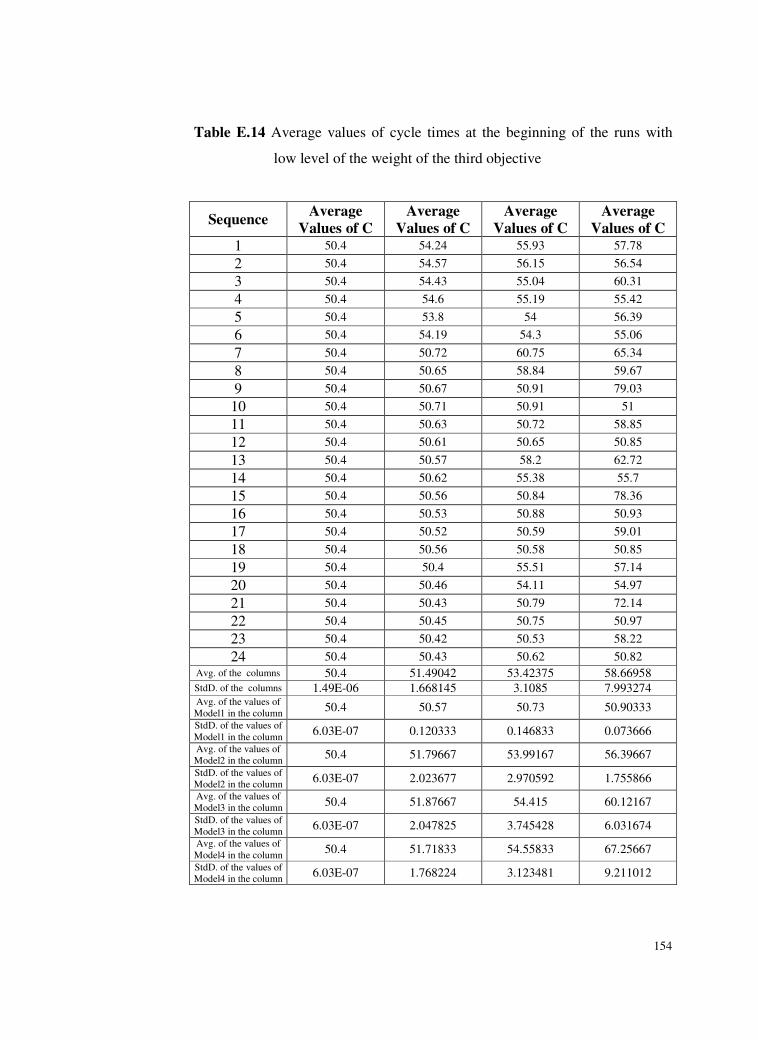
154
Table E.14 Average values of cycle times at the beginning of the runs with
low level of the weight of the third objective
Sequence Average
Values of C
Average
Values of C
Average
Values of C
Average
Values of C
1 50.4 54.24 55.93 57.78
2 50.4 54.57 56.15 56.54
3 50.4 54.43 55.04 60.31
4 50.4 54.6 55.19 55.42
5 50.4 53.8 54 56.39
6 50.4 54.19 54.3 55.06
7 50.4 50.72 60.75 65.34
8 50.4 50.65 58.84 59.67
9 50.4 50.67 50.91 79.03
10 50.4 50.71 50.91 51
11 50.4 50.63 50.72 58.85
12 50.4 50.61 50.65 50.85
13 50.4 50.57 58.2 62.72
14 50.4 50.62 55.38 55.7
15 50.4 50.56 50.84 78.36
16 50.4 50.53 50.88 50.93
17 50.4 50.52 50.59 59.01
18 50.4 50.56 50.58 50.85
19 50.4 50.4 55.51 57.14
20 50.4 50.46 54.11 54.97
21 50.4 50.43 50.79 72.14
22 50.4 50.45 50.75 50.97
23 50.4 50.42 50.53 58.22
24 50.4 50.43 50.62 50.82
Avg. of the columns 50.4 51.49042 53.42375 58.66958
StdD. of the columns 1.49E-06 1.668145 3.1085 7.993274 Avg. of the values of
Model1 in the column 50.4 50.57 50.73 50.90333
StdD. of the values of
Model1 in the column 6.03E-07 0.120333 0.146833 0.073666
Avg. of the values of
Model2 in the column 50.4 51.79667 53.99167 56.39667
StdD. of the values of
Model2 in the column 6.03E-07 2.023677 2.970592 1.755866
Avg. of the values of
Model3 in the column 50.4 51.87667 54.415 60.12167
StdD. of the values of
Model3 in the column 6.03E-07 2.047825 3.745428 6.031674
Avg. of the values of
Model4 in the column 50.4 51.71833 54.55833 67.25667
StdD. of the values of
Model4 in the column 6.03E-07 1.768224 3.123481 9.211012

155
Table E.15 Average values of cycle times at the end of the runs with low level
of the weight of the third objective
Sequence Average
Values of C
Average
Values of C
Average
Values of C
Average
Values of C
1 48.75 52.58 54.99 56.62
2 48.61 53.01 55.41 55.17
3 48.67 53.28 53.25 58.57
4 48.6 53.5 54.29 53.79
5 48.94 52.82 52.42 54.57
6 48.78 53.58 53.15 53.23
7 48.64 48.56 58.45 63.8
8 49.06 48.88 57.22 57.63
9 48.93 48.79 48.9 72.92
10 48.73 49.18 49.57 48.81
11 49.12 49.14 49.56 57.22
12 49.32 49.69 49.26 48.95
13 48.99 48.38 56.66 60.72
14 48.44 49.26 54.37 54.84
15 49.05 49.12 48.87 73.78
16 49.3 48.85 50.13 49.03
17 49.33 49.51 48.77 57.21
18 49.06 50.08 49.3 49.1
19 49.88 48.61 54.45 55.31
20 49.39 49.15 52.79 54.11
21 49.76 48.55 47.74 69.56
22 49.31 48.92 49.13 49.29
23 49.87 49.5 48.89 56.93
24 49.61 48.92 49.74 49.19
Avg. of the columns 49.08917 50.0775 51.97125 56.68125
StdD. of the columns 0.412858 1.847502 3.181611 7.166972 Avg. of the values of
Model1 in the column 48.725 48.80667 48.78833 49.06167
StdD. of the values of
Model1 in the column 0.127867 0.34938 0.587245 0.171396
Avg. of the values of
Model2 in the column 48.96667 50.17167 52.63667 55.01833
StdD. of the values of
Model2 in the column 0.25343 2.044773 2.807936 1.674615
Avg. of the values of
Model3 in the column 49.02833 50.52833 52.96167 58.24333
StdD. of the values of
Model3 in the column 0.320588 2.230986 3.540759 5.675095
Avg. of the values of
Model4 in the column 49.63667 50.80333 53.49833 64.40167
StdD. of the values of
Model4 in the column 0.243776 1.896256 3.022227 7.334773

156
Table E.16 Average values of the differences between the theoretical
minimum cycle times and the cycle times found with the
algorithm at the end of the runs with low level of the weight of
the third objective
Sequence Average
Values of DC
Average
Values of DC
Average
Values of DC
Average
Values of DC
1 0.30795 0.250227 0.170246 0.221553
2 0.253025 0.218548 0.212771 0.164664
3 0.258121 0.236712 0.213808 0.221296
4 0.267079 0.184502 0.181199 0.207559
5 0.309051 0.206442 0.250292 0.177622
6 0.238013 0.174031 0.229356 0.283235
7 0.255518 0.277753 0.242591 0.236192
8 0.261656 0.274713 0.23215 0.222138
9 0.250552 0.218513 0.306297 0.204431
10 0.275927 0.220764 0.235347 0.269777
11 0.251538 0.212709 0.300449 0.209892
12 0.268215 0.231884 0.227516 0.280701
13 0.220762 0.263228 0.209686 0.211952
14 0.204259 0.306019 0.192271 0.242804
15 0.238766 0.251785 0.303608 0.246848
16 0.215431 0.258287 0.226374 0.272556
17 0.188039 0.244323 0.295886 0.224421
18 0.225333 0.250407 0.280798 0.262885
19 0.247797 0.282342 0.311987 0.199894
20 0.234063 0.282939 0.220304 0.226846
21 0.237507 0.19037 0.226057 0.303527
22 0.213728 0.264037 0.230603 0.278558
23 0.232965 0.232173 0.30538 0.275813
24 0.197259 0.214413 0.274551 0.285112
Avg. of the columns 0.243857 0.239463 0.24498 0.238762
StdD. of the columns 0.030318 0.03381 0.042327 0.036995 Avg. of the values of
Model1 in the column 0.272206 0.281166 0.289613 0.274931
StdD. of the values of
Model1 in the column 0.029654 0.014123 0.031365 0.008092
Avg. of the values of
Model2 in the column 0.260568 0.238876 0.256854 0.243446
StdD. of the values of
Model2 in the column 0.010029 0.028536 0.040117 0.030188
Avg. of the values of
Model3 in the column 0.215432 0.217846 0.220103 0.212956
StdD. of the values of
Model3 in the column 0.017585 0.018405 0.025465 0.049088
Avg. of the values of
Model4 in the column 0.22722 0.219966 0.213352 0.223712
StdD. of the values of Model4 in the column
0.018378 0.028311 0.022295 0.015566

157
Table E.17 Average values of TSTs at the beginning of the runs with
intermediate level of the weight of the third objective
Sequence
Average
Values of
TST
Average
Values of
TST
Average
Values of
TST
Average
Values of
TST
1 256.2 313.22 318.65 329.15
2 256.2 296.93 265.11 279.11
3 256.2 302.47 304.07 322.97
4 256.2 317.61 327.35 310.69
5 256.2 326.3 327.11 319.24
6 256.2 284.18 285.02 293.37
7 242 261.52 313.69 331.53
8 242 263.76 289.04 289.62
9 242 275.2 265.44 303.6
10 242 268.37 264.84 263.48
11 242 283.5 262.36 284.44
12 242 274.03 278.84 264.04
13 292.08 260.4 300.45 297.76
14 287.04 263.76 302.77 303.04
15 292.08 247.8 263.2 328.34
16 282 244.61 277.17 260.96
17 297.12 286 260.12 305.79
18 271.92 271.16 247.22 262.64
19 256.64 257.6 309.32 302.72
20 266.72 257.88 289.56 308.62
21 256.64 242.87 260.4 306.66
22 261.68 242.87 280.98 263.76
23 261.68 293.24 257.88 293.88
24 276.8 278.68 245.19 260.12
Avg. of the columns 262.15 275.5817 283.1575 295.2304
StdD. of the columns 17.53099 23.58185 24.88857 23.42245 Avg. of the values of
Model1 in the column 256.2 260.82 261.5667 262.5
StdD. of the values of
Model1 in the column 0 2.719029 2.658772 1.610913
Avg. of the values of
Model2 in the column 242 264.7167 288.8933 302.565
StdD. of the values of
Model2 in the column 0 31.73414 34.31705 7.392999
Avg. of the values of
Model3 in the column 287.04 289.2617 294.4567 296.965
StdD. of the values of
Model3 in the column 9.015826 18.65518 17.28449 15.18496
Avg. of the values of
Model4 in the column 263.36 287.5283 287.7133 318.8917
StdD. of the values of Model4 in the column
7.587948 19.91554 24.26846 14.49998
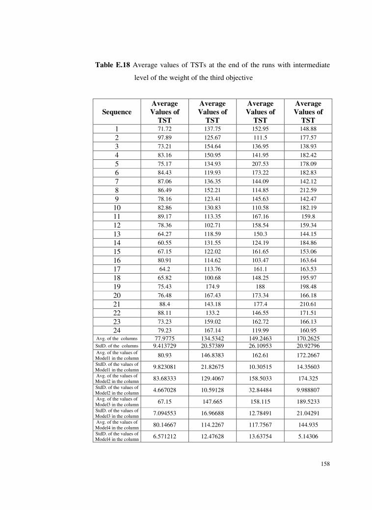
158
Table E.18 Average values of TSTs at the end of the runs with intermediate
level of the weight of the third objective
Sequence
Average
Values of
TST
Average
Values of
TST
Average
Values of
TST
Average
Values of
TST
1 71.72 137.75 152.95 148.88
2 97.89 125.67 111.5 177.57
3 73.21 154.64 136.95 138.93
4 83.16 150.95 141.95 182.42
5 75.17 134.93 207.53 178.09
6 84.43 119.93 173.22 182.83
7 87.06 136.35 144.09 142.12
8 86.49 152.21 114.85 212.59
9 78.16 123.41 145.63 142.47
10 82.86 130.83 110.58 182.19
11 89.17 113.35 167.16 159.8
12 78.36 102.71 158.54 159.34
13 64.27 118.59 150.3 144.15
14 60.55 131.55 124.19 184.86
15 67.15 122.02 161.65 153.06
16 80.91 114.62 103.47 163.64
17 64.2 113.76 161.1 163.53
18 65.82 100.68 148.25 195.97
19 75.43 174.9 188 198.48
20 76.48 167.43 173.34 166.18
21 88.4 143.18 177.4 210.61
22 88.11 133.2 146.55 171.51
23 73.23 159.02 162.72 166.13
24 79.23 167.14 119.99 160.95
Avg. of the columns 77.9775 134.5342 149.2463 170.2625
StdD. of the columns 9.413729 20.57389 26.10953 20.92796 Avg. of the values of
Model1 in the column 80.93 146.8383 162.61 172.2667
StdD. of the values of
Model1 in the column 9.823081 21.82675 10.30515 14.35603
Avg. of the values of
Model2 in the column 83.68333 129.4067 158.5033 174.325
StdD. of the values of
Model2 in the column 4.667028 10.59128 32.84484 9.988807
Avg. of the values of
Model3 in the column 67.15 147.665 158.115 189.5233
StdD. of the values of
Model3 in the column 7.094553 16.96688 12.78491 21.04291
Avg. of the values of
Model4 in the column 80.14667 114.2267 117.7567 144.935
StdD. of the values of Model4 in the column
6.571212 12.47628 13.63754 5.14306

159
Table E.19 Average values of numbers of stations at the beginning of the runs
with intermediate level of the weight of the third objective
Sequence Average
Values of m
Average
Values of m
Average
Values of m
Average
Values of m
1 34 34 32.8 34.6
2 34 34.7 36.1 33.4
3 34 32.9 33.5 35.2
4 34 33.2 35.9 33.5
5 34 36 33.9 32.6
6 34 36.2 33.3 34
7 35 34 33.7 35.5
8 35 34 36.5 33.5
9 35 34.7 34 34.7
10 35 34.6 37.6 34
11 35 38 34 32.6
12 35 37.8 34.8 34
13 35.2 34 34.9 36.2
14 35.1 34 36.7 34.5
15 35.2 35 34 35.6
16 35 35 37.9 34
17 35.3 38.1 34 34.9
18 34.8 37.8 35 34
19 37.6 34 34.7 33.1
20 37.8 34 33.7 34.5
21 37.6 35 34 33.1
22 37.7 35 34.9 34
23 37.7 35.2 34 34.6
24 38 34.9 35 34
Avg. of the columns 35.45833 35.0875 34.7875 34.17083
StdD. of the columns 1.416031 1.497625 1.350785 0.916268 Avg. of the values of
Model1 in the column 34 34 34 34
StdD. of the values of
Model1 in the column 0 0 0 0
Avg. of the values of
Model2 in the column 35 34.78333 34.5 34.33333
StdD. of the values of
Model2 in the column 0 0.402078 0.641872 0.500666
Avg. of the values of
Model3 in the column 35.1 34.25 33.86667 33.05
StdD. of the values of
Model3 in the column 0.178885 0.956556 0.831064 0.383406
Avg. of the values of
Model4 in the column 37.73333 37.31667 36.78333 35.3
StdD. of the values of
Model4 in the column 0.150555 0.951665 0.806019 0.6

160
Table E.20 Average values of numbers of stations at the end of the runs with
intermediate level of the weight of the third objective
Sequence Average
Values of m
Average
Values of m
Average
Values of m
Average
Values of m
1 31.3 31.3 30.5 31.8
2 31.4 31.6 33.3 31.7
3 31.4 30.5 30.7 32.3
4 31.6 30.6 32.8 31.4
5 31.5 32.8 32 30.7
6 31.3 33.3 31.5 32.1
7 32.5 31.9 31.2 32.4
8 32.7 32.1 33.4 32.3
9 32.6 31.9 31.9 32.2
10 32.5 32 34.6 32.6
11 32.6 34.7 32.5 30.9
12 32.4 34.5 32.6 32.1
13 31.3 31.5 32.3 33.5
14 31.8 31.8 33.5 32.6
15 31.6 32.7 32.2 32.7
16 31.4 32.6 34.5 32.3
17 31.2 34.8 32.3 32.6
18 31.4 34.5 33.2 32.9
19 34.6 32.9 32.9 31.8
20 34.8 32.7 31.9 32.3
21 34.8 33.3 32.7 31.6
22 34.8 33.1 32.6 32.6
23 34.4 32.7 32.4 32.5
24 34.7 32.9 32.6 32.2
Avg. of the columns 32.525 32.6125 32.50417 32.17083
StdD. of the columns 1.36326 1.188464 0.994541 0.616779 Avg. of the values of
Model1 in the column 31.41667 32.15 32.33333 32.45
StdD. of the values of
Model1 in the column 0.116905 0.543139 0.273252 0.301662
Avg. of the values of
Model2 in the column 32.55 32.43333 32.28333 32.25
StdD. of the values of
Model2 in the column 0.104881 0.809115 0.884119 0.459347
Avg. of the values of
Model3 in the column 31.45 31.76667 31.71667 31.5
StdD. of the values of
Model3 in the column 0.216795 1.01915 0.823205 0.596657
Avg. of the values of
Model4 in the column 34.68333 34.1 33.68333 32.48333
StdD. of the values of
Model4 in the column 0.160208 0.83666 0.713909 0.577639

161
Table E.21 Average values of the differences between the theoretical
minimum numbers of used stations and the numbers of used
stations found with the algorithm at the end of the runs with
intermediate level of the weight of the third objective
Sequence Average
Values of Dm
Average
Values of Dm
Average
Values of Dm
Average
Values of Dm
1 1.478763 2.564699 2.811064 2.560275
2 1.984391 2.389163 2.100999 3.35798
3 1.513541 2.839515 2.490453 2.472944
4 1.718892 2.789688 2.571092 3.299928
5 1.557927 2.456399 3.776706 3.237411
6 1.723061 2.24546 3.260919 3.396433
7 1.765565 2.734657 2.739354 2.522542
8 1.767989 3.03873 2.165347 4.008863
9 1.601639 2.452991 2.899841 2.502547
10 1.685517 2.595833 2.18624 3.624229
11 1.81203 2.244554 3.3499 2.93696
12 1.593655 2.034667 3.151262 3.164019
13 1.307098 2.374174 2.885945 2.674893
14 1.259098 2.637858 2.336155 3.496501
15 1.378567 2.428259 3.216915 2.741046
16 1.630264 2.285088 2.048505 3.263662
17 1.300385 2.259833 3.219424 3.143599
18 1.34217 1.997223 2.947902 3.90223
19 1.52816 3.537621 3.592586 3.714072
20 1.558907 3.380376 3.315608 3.151527
21 1.786942 2.868189 3.55511 3.864404
22 1.78144 2.668269 2.93923 3.439142
23 1.475519 3.17152 3.258963 3.175875
24 1.606448 3.338127 2.382645 3.20426
Avg. of the columns 1.589915 2.638871 2.883423 3.202306
StdD. of the columns 0.187076 0.418258 0.505731 0.452205 Avg. of the values of
Model1 in the column 1.662763 2.950569 3.250026 3.432924
StdD. of the values of
Model1 in the column 0.188332 0.450283 0.213445 0.286402
Avg. of the values of
Model2 in the column 1.704399 2.533945 3.012706 3.27731
StdD. of the values of
Model2 in the column 0.092249 0.212023 0.567442 0.146107
Avg. of the values of
Model3 in the column 1.369597 2.864612 3.036239 3.519948
StdD. of the values of
Model3 in the column 0.13393 0.336549 0.240838 0.410197
Avg. of the values of
Model4 in the column 1.622903 2.206356 2.234723 2.579041
StdD. of the values of Model4 in the column
0.13199 0.168276 0.191393 0.105911

162
Table E.22 Average values of cycle times at the beginning of the runs with
intermediate level of the weight of the third objective
Sequence Average
Values of C
Average
Values of C
Average
Values of C
Average
Values of C
1 50.4 54.82 55.97 59.05
2 50.4 52.89 53.2 53.28
3 50.4 55.15 55.5 56.93
4 50.4 55.11 55.64 55.74
5 50.4 55.41 55.5 56.38
6 50.4 53.67 53.72 54.12
7 50.4 50.59 54.01 56.83
8 50.4 50.67 53.32 53.49
9 50.4 50.69 50.73 57.9
10 50.4 50.63 50.66 50.66
11 50.4 50.61 50.62 55.65
12 50.4 50.63 50.64 50.68
13 50.4 50.55 52.61 54.12
14 50.4 50.67 53.43 53.49
15 50.4 50.6 50.65 56.33
16 50.4 50.49 50.57 50.57
17 50.4 50.53 50.54 52.79
18 50.4 50.54 50.58 50.63
19 50.4 50.45 53.31 54.78
20 50.4 50.46 53.1 53.67
21 50.4 50.43 50.55 55.1
22 50.4 50.43 50.54 50.67
23 50.4 50.44 50.46 53.03
24 50.4 50.46 50.51 50.54
Avg. of the columns 50.4 51.53833 52.34833 54.01792
StdD. of the columns 1.49E-06 1.81435 1.979527 2.535847 Avg. of the values of
Model1 in the column 50.4 50.565 50.59167 50.625
StdD. of the values of
Model1 in the column 6.03E-07 0.097108 0.094956 0.057533
Avg. of the values of
Model2 in the column 50.4 51.61 53.00167 53.80667
StdD. of the values of
Model2 in the column 6.03E-07 1.844007 2.227316 1.057519
Avg. of the values of
Model3 in the column 50.4 52.08 52.99667 54.78
StdD. of the values of
Model3 in the column 6.03E-07 2.364504 2.097166 1.211066
Avg. of the values of
Model4 in the column 50.4 51.89833 52.80333 56.86
StdD. of the values of
Model4 in the column 6.03E-07 2.119268 1.920694 1.653602

163
Table E.23 Average values of cycle times at the end of the runs with
intermediate level of the weight of the third objective
Sequence Average
Values of C
Average
Values of C
Average
Values of C
Average
Values of C
1 48.5 53.71 54.41 58.15
2 49.33 52.6 53.07 52.88
3 48.37 54.46 54.99 56.18
4 48.38 54.11 55.21 55.28
5 48.25 54.93 54.95 55.01
6 49 53.41 53.12 53.83
7 49.31 49.86 52.6 56.34
8 48.92 50.09 53.04 53.03
9 48.8 50.31 50.22 56.93
10 49.16 50.4 50.58 50.27
11 49.21 50.5 49.9 54.41
12 49.17 50.48 50.31 50.36
13 49.17 49.95 52.08 53.89
14 48.09 49.87 53.16 52.87
15 48.71 50.25 50.25 55.84
16 49.63 50.16 50.51 50.14
17 49.37 50.34 50.04 52.02
18 49.04 50.41 50.29 50.22
19 49.36 49.44 52.33 53.44
20 49.06 49.53 52.28 52.73
21 49.47 49.92 49.9 54.5
22 49.46 49.92 49.86 49.87
23 49.63 50.14 49.93 52.31
24 49.32 50.07 50.36 50.23
Avg. of the columns 49.02958 51.03583 51.80792 53.36375
StdD. of the columns 0.440568 1.734775 1.849945 2.401255 Avg. of the values of
Model1 in the column 48.63833 49.79 50.04 50.18167
StdD. of the values of
Model1 in the column 0.428458 0.251794 0.159875 0.168691
Avg. of the values of
Model2 in the column 49.095 51.09333 52.5 53.17333
StdD. of the values of
Model2 in the column 0.193365 1.640289 2.091488 1.202775
Avg. of the values of
Model3 in the column 49.00167 51.58167 52.09667 53.87833
StdD. of the values of
Model3 in the column 0.543412 2.100204 1.72514 0.87844
Avg. of the values of
Model4 in the column 49.38333 51.67833 52.595 56.22167
StdD. of the values of
Model4 in the column 0.191485 1.989788 1.788214 1.401305

164
Table E.24 Average values of the differences between the theoretical
minimum cycle times and the cycle times found with the
algorithm at the end of the runs with intermediate level of the
weight of the third objective
Sequence Average
Values of DC
Average
Values of DC
Average
Values of DC
Average
Values of DC
1 0.229137 0.440096 0.501475 0.468176
2 0.311752 0.39769 0.334835 0.560158
3 0.233153 0.507016 0.446091 0.430124
4 0.263165 0.493301 0.432774 0.580955
5 0.238635 0.411372 0.648531 0.580098
6 0.269744 0.36015 0.549905 0.569564
7 0.267877 0.427429 0.461827 0.438642
8 0.264495 0.474174 0.343862 0.658173
9 0.239755 0.386865 0.45652 0.442453
10 0.254954 0.408844 0.319595 0.558865
11 0.273528 0.326657 0.514338 0.517152
12 0.241852 0.29771 0.486319 0.496386
13 0.205335 0.376476 0.465325 0.430299
14 0.190409 0.413679 0.370716 0.567055
15 0.2125 0.37315 0.502019 0.468073
16 0.257675 0.351595 0.299913 0.506625
17 0.205769 0.326897 0.498762 0.501626
18 0.209618 0.291826 0.446536 0.595653
19 0.218006 0.531611 0.571429 0.624151
20 0.21977 0.512018 0.543386 0.514489
21 0.254023 0.42997 0.542508 0.666487
22 0.25319 0.402417 0.44954 0.526104
23 0.212878 0.4863 0.502222 0.511169
24 0.228329 0.508024 0.368067 0.499845
Avg. of the columns 0.239814 0.41397 0.460687 0.52968
StdD. of the columns 0.028303 0.069749 0.086577 0.067813 Avg. of the values of
Model1 in the column 0.257598 0.455898 0.502728 0.53058
StdD. of the values of
Model1 in the column 0.031236 0.060194 0.027817 0.039351
Avg. of the values of
Model2 in the column 0.257077 0.399153 0.490997 0.54081
StdD. of the values of
Model2 in the column 0.013991 0.033397 0.101045 0.03531
Avg. of the values of
Model3 in the column 0.213551 0.465058 0.498742 0.601037
StdD. of the values of
Model3 in the column 0.022922 0.053159 0.041367 0.058701
Avg. of the values of
Model4 in the column 0.231032 0.335769 0.350283 0.446295
StdD. of the values of Model4 in the column
0.018182 0.044388 0.046864 0.017572

165
Table E.25 Average values of TSTs at the beginning of the runs with high
level of the weight of the third objective
Sequence
Average
Values of
TST
Average
Values of
TST
Average
Values of
TST
Average
Values of
TST
1 256.2 308.33 336.28 325.2
2 256.2 334 307.17 323.53
3 256.2 328.46 364.82 346.1
4 256.2 304.62 335.9 303.62
5 256.2 313.61 348.2 301.57
6 256.2 296.98 313.63 338.53
7 242 269.64 317.45 374.09
8 242 266.84 311.12 348.64
9 242 257.73 271.32 338.4
10 242 260.58 268.4 276.64
11 242 274.7 264.04 332.64
12 242 256.49 267.05 274.12
13 292.08 263.2 312.39 341.16
14 276.96 264.04 294.41 296.28
15 297.12 246.64 263.2 333.17
16 292.08 246.64 269.89 263.76
17 292.08 274.34 263.48 329.08
18 276.96 258.84 249.25 264.04
19 256.64 257.32 306.24 320.11
20 271.76 257.6 298.18 317.64
21 286.88 242.87 262.08 314.17
22 256.64 243.74 275.22 269.08
23 271.76 288.49 261.24 345.11
24 281.84 273.64 247.51 266
Avg. of the columns 264.25 274.5558 292.0196 314.2783
StdD. of the columns 18.80841 26.52214 33.08313 31.5232 Avg. of the values of
Model1 in the column 256.2 263.1067 264.2267 268.94
StdD. of the values of
Model1 in the column 0 4.925666 3.61912 5.396814
Avg. of the values of
Model2 in the column 242 270.37 304.735 321.71
StdD. of the values of
Model2 in the column 0 40.20291 48.81304 19.3664
Avg. of the values of
Model3 in the column 287.88 285.5867 301.3017 323.4433
StdD. of the values of
Model3 in the column 8.680903 27.39661 26.4553 16.09352
Avg. of the values of
Model4 in the column 270.92 279.16 297.815 343.02
StdD. of the values of Model4 in the column
12.51572 22.24549 25.96786 16.81791
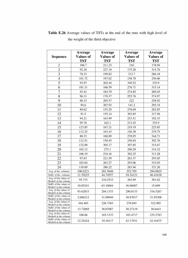
166
Table E.26 Average values of TSTs at the end of the runs with high level of
the weight of the third objective
Sequence
Average
Values of
TST
Average
Values of
TST
Average
Values of
TST
Average
Values of
TST
1 106.7 211.23 216 178.94
2 92.26 227.18 175.26 314.76
3 78.33 199.82 313.7 286.18
4 101.72 197.62 158.78 256.06
5 93.97 202.44 349.52 335.9
6 101.31 166.59 276.71 315.14
7 93.41 184.79 274.85 269.45
8 96.31 170.37 255.76 374.97
9 96.33 205.57 222 258.92
10 94.6 207.93 141.2 295.34
11 89.62 155.29 278.69 282.85
12 91.5 155.14 303.85 317.56
13 94.21 163.99 253.51 192.33
14 95.76 162.1 213.45 335.9
15 123.85 167.21 219.19 225.85
16 112.25 163.43 156.38 279.75
17 88.33 160.89 278.95 344.71
18 112.51 150.45 256.84 302.76
19 132.09 305.17 307.85 315.67
20 102.12 275.1 290.29 314.32
21 106.19 234.16 302.25 313.28
22 97.83 221.59 263.37 293.05
23 103.04 263.27 293.06 333.03
24 110.69 286.22 263.46 321.26
Avg. of the columns 100.6221 201.5646 252.705 294.0825
StdD. of the columns 11.70225 44.74557 54.54121 46.41638 Avg. of the values of
Model1 in the column 95.715 210.2533 265.69 301.62
StdD. of the values of
Model1 in the column 10.05241 63.10684 36.06007 15.699
Avg. of the values of
Model2 in the column 93.62833 204.1333 290.8133 316.5267
StdD. of the values of
Model2 in the column 2.686212 31.00949 38.87017 31.95308
Avg. of the values of
Model3 in the column 104.485 226.7383 270.845 322.905
StdD. of the values of
Model3 in the column 13.72869 38.07087 30.27119 30.6443
Avg. of the values of
Model4 in the column 108.66 165.1333 183.4717 235.2783
StdD. of the values of Model4 in the column
12.25424 19.10117 43.17931 43.41675
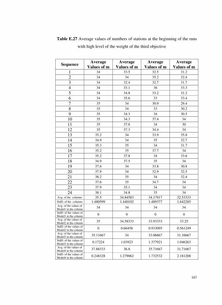
167
Table E.27 Average values of numbers of stations at the beginning of the runs
with high level of the weight of the third objective
Sequence Average
Values of m
Average
Values of m
Average
Values of m
Average
Values of m
1 34 33.5 32.5 31.2
2 34 34 35.2 32.4
3 34 32.4 32.7 31.7
4 34 33.1 36 33.3
5 34 34.8 33.2 31.2
6 34 35.6 33 33.4
7 35 34 30.9 29.4
8 35 34 33 30.2
9 35 34.3 34 30.5
10 35 34.3 37.4 34
11 35 37.8 34 30
12 35 37.3 34.4 34
13 35.2 34 33.9 35.8
14 34.9 34 35 32.7
15 35.3 35 34 31.7
16 35.2 35 37.7 34
17 35.2 37.8 34 33.6
18 34.9 37.5 35 34
19 37.6 34 33.8 30.8
20 37.9 34 32.9 32.5
21 38.2 35 34 32.4
22 37.6 35 34.7 34
23 37.9 35.1 34 34
24 38.1 34.8 35 34
Avg. of the columns 35.5 34.84583 34.17917 32.53333
StdD. of the columns 1.480599 1.440102 1.489377 1.642285 Avg. of the values of
Model1 in the column 34 34 34 34
StdD. of the values of
Model1 in the column 0 0 0 0
Avg. of the values of
Model2 in the column 35 34.58333 33.93333 33.25
StdD. of the values of
Model2 in the column 0 0.66458 0.933095 0.561249
Avg. of the values of
Model3 in the column 35.11667 34 33.06667 31.16667
StdD. of the values of
Model3 in the column 0.17224 1.03923 1.377921 1.046263
Avg. of the values of
Model4 in the column 37.88333 36.8 35.71667 31.71667
StdD. of the values of
Model4 in the column 0.248328 1.279062 1.732532 2.181208
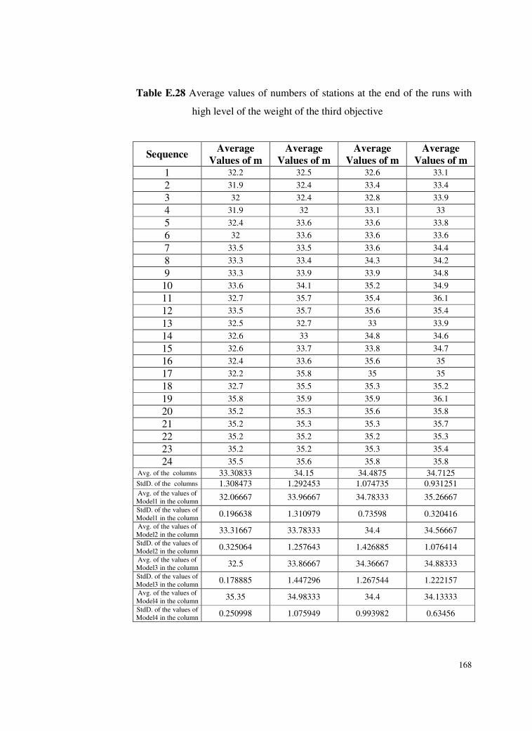
168
Table E.28 Average values of numbers of stations at the end of the runs with
high level of the weight of the third objective
Sequence Average
Values of m
Average
Values of m
Average
Values of m
Average
Values of m
1 32.2 32.5 32.6 33.1
2 31.9 32.4 33.4 33.4
3 32 32.4 32.8 33.9
4 31.9 32 33.1 33
5 32.4 33.6 33.6 33.8
6 32 33.6 33.6 33.6
7 33.5 33.5 33.6 34.4
8 33.3 33.4 34.3 34.2
9 33.3 33.9 33.9 34.8
10 33.6 34.1 35.2 34.9
11 32.7 35.7 35.4 36.1
12 33.5 35.7 35.6 35.4
13 32.5 32.7 33 33.9
14 32.6 33 34.8 34.6
15 32.6 33.7 33.8 34.7
16 32.4 33.6 35.6 35
17 32.2 35.8 35 35
18 32.7 35.5 35.3 35.2
19 35.8 35.9 35.9 36.1
20 35.2 35.3 35.6 35.8
21 35.2 35.3 35.3 35.7
22 35.2 35.2 35.2 35.3
23 35.2 35.2 35.3 35.4
24 35.5 35.6 35.8 35.8
Avg. of the columns 33.30833 34.15 34.4875 34.7125
StdD. of the columns 1.308473 1.292453 1.074735 0.931251 Avg. of the values of
Model1 in the column 32.06667 33.96667 34.78333 35.26667
StdD. of the values of
Model1 in the column 0.196638 1.310979 0.73598 0.320416
Avg. of the values of
Model2 in the column 33.31667 33.78333 34.4 34.56667
StdD. of the values of
Model2 in the column 0.325064 1.257643 1.426885 1.076414
Avg. of the values of
Model3 in the column 32.5 33.86667 34.36667 34.88333
StdD. of the values of
Model3 in the column 0.178885 1.447296 1.267544 1.222157
Avg. of the values of
Model4 in the column 35.35 34.98333 34.4 34.13333
StdD. of the values of
Model4 in the column 0.250998 1.075949 0.993982 0.63456
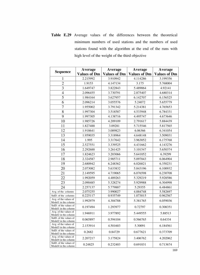
169
Table E.29 Average values of the differences between the theoretical
minimum numbers of used stations and the numbers of used
stations found with the algorithm at the end of the runs with
high level of the weight of the third objective
Sequence Average
Values of Dm
Average
Values of Dm
Average
Values of Dm
Average
Values of Dm
1 2.215992 3.910942 4.114286 3.199356
2 1.9153 4.147134 3.175 5.768004
3 1.649747 3.822843 5.489064 4.92141
4 2.096455 3.730791 2.875407 4.680314
5 1.984164 3.627957 6.142707 6.156525
6 2.096214 3.055576 5.24072 5.655779
7 1.955002 3.791342 5.214381 4.765653
8 1.997304 3.518587 4.533948 6.784331
9 1.997305 4.138716 4.495747 4.673646
10 1.985726 4.209109 2.791617 5.884439
11 1.827488 3.09281 5.715546 5.817565
12 1.918641 3.089823 6.06366 6.341054
13 1.959035 3.318964 4.648148 3.509031
14 1.995 3.317642 3.963052 6.175768
15 2.527551 3.339525 4.431662 4.143276
16 2.292688 3.261425 3.101547 5.650374
17 1.824623 3.203066 5.641052 6.39299
18 2.324587 2.985711 5.097043 6.064904
19 2.680942 6.248362 6.026821 6.350231
20 2.073082 5.633832 5.843196 6.100932
21 2.149595 4.719065 6.076598 6.230708
22 1.992059 4.489263 5.329219 5.928586
23 2.090485 5.328274 5.929988 6.304998
24 2.257137 5.779887 5.29355 6.484861
Avg. of the columns 2.075255 3.990027 4.884748 5.582697
StdD. of the columns 0.225117 0.935749 1.073015 0.962567 Avg. of the values of
Model1 in the column 1.992979 4.304788 5.381765 6.059036
StdD. of the values of
Model1 in the column 0.197494 1.293977 0.72797 0.308351
Avg. of the values of
Model2 in the column 1.946911 3.977892 5.449555 5.88513
StdD. of the values of
Model2 in the column 0.065897 0.594104 0.566765 0.64334
Avg. of the values of
Model3 in the column 2.153914 4.501603 5.30091 6.184561
StdD. of the values of
Model3 in the column 0.2682 0.84729 0.677621 0.373709
Avg. of the values of
Model4 in the column 2.207217 3.175824 3.406762 4.202062
StdD. of the values of Model4 in the column
0.24825 0.232403 0.691031 0.713674

170
Table E.30 Average values of cycle times at the beginning of the runs with
high level of the weight of the third objective
Sequence Average
Values of C
Average
Values of C
Average
Values of C
Average
Values of C
1 50.4 55.64 57.3 66.87
2 50.4 55.6 56.43 57.06
3 50.4 57.2 59.71 67.29
4 50.4 54.78 55.73 55.86
5 50.4 57.49 57.83 59.24
6 50.4 55.23 55.37 57.08
7 50.4 50.88 60.76 76.88
8 50.4 50.78 61.81 64.55
9 50.4 50.79 50.94 72.65
10 50.4 50.89 51.1 51.13
11 50.4 50.65 50.68 64.04
12 50.4 50.88 50.94 51.04
13 50.4 50.65 55.03 56.46
14 50.4 50.68 57 58.04
15 50.4 50.56 50.65 67.35
16 50.4 50.56 50.66 50.67
17 50.4 50.64 50.66 56.23
18 50.4 50.63 50.65 50.68
19 50.4 50.44 54.99 60.9
20 50.4 50.45 55.02 58.58
21 50.4 50.43 50.61 56.71
22 50.4 50.46 50.69 50.86
23 50.4 50.45 50.58 56.01
24 50.4 50.46 50.59 50.75
Avg. of the columns 50.4 51.9675 53.98875 59.03875
StdD. of the columns 1.49E-06 2.431021 3.708968 7.256734 Avg. of the values of
Model1 in the column 50.4 50.64667 50.68667 50.855
StdD. of the values of
Model1 in the column 6.03E-07 0.175917 0.129254 0.192743
Avg. of the values of
Model2 in the column 50.4 52.20833 54.8 56.96667
StdD. of the values of
Model2 in the column 6.03E-07 2.643213 3.696609 1.135811
Avg. of the values of
Model3 in the column 50.4 52.42833 55.01333 60.41667
StdD. of the values of
Model3 in the column 6.03E-07 2.868375 3.838321 3.371579
Avg. of the values of
Model4 in the column 50.4 52.58667 55.455 67.91667
StdD. of the values of
Model4 in the column 6.03E-07 3.01036 4.141433 6.867464

171
Table E.31 Average values of cycle times at the end of the runs with high level
of the weight of the third objective
Sequence Average
Values of C
Average
Values of C
Average
Values of C
Average
Values of C
1 48.15 54.01 52.5 55.93
2 48.17 54.78 55.2 54.57
3 47.48 52.27 57.15 58.15
4 48.52 52.97 55.22 54.71
5 47.36 55.8 56.9 54.56
6 48.33 54.52 52.8 55.72
7 47.78 48.74 52.71 56.54
8 48.22 48.42 56.41 55.27
9 48.23 49.67 49.38 55.4
10 47.64 49.4 50.58 50.19
11 49.04 50.21 48.76 48.62
12 47.69 50.21 50.11 50.08
13 48.09 49.41 54.54 54.81
14 48 48.86 53.86 54.39
15 49 50.07 49.46 54.51
16 48.96 50.11 50.42 49.51
17 48.41 50.23 49.45 53.92
18 48.4 50.39 50.39 49.92
19 49.27 48.84 51.08 49.71
20 49.26 48.83 49.68 51.52
21 49.4 49.62 49.74 50.28
22 49.11 49.36 49.42 49.43
23 49.29 49.41 49.42 52.82
24 49.04 49.52 49.77 49.54
Avg. of the columns 48.45167 50.65208 51.87292 52.92083
StdD. of the columns 0.627893 2.158153 2.73561 2.831441 Avg. of the values of
Model1 in the column 48.00167 48.85 49.36833 49.77833
StdD. of the values of
Model1 in the column 0.471314 0.31975 0.324371 0.325786
Avg. of the values of
Model2 in the column 48.1 51.325 53.305 53.84667
StdD. of the values of
Model2 in the column 0.528583 2.406896 3.321968 1.484772
Avg. of the values of
Model3 in the column 48.47667 50.54 51.20333 52.16833
StdD. of the values of
Model3 in the column 0.422974 1.629208 1.624619 2.943069
Avg. of the values of
Model4 in the column 49.22833 51.89333 53.615 55.89
StdD. of the values of
Model4 in the column 0.130754 2.563409 2.544781 1.329857

172
Table E.32 Average values of the differences between the theoretical
minimum cycle times and the cycle times found with the
algorithm at the end of the runs with high level of the weight of
the third objective
Sequence Average
Values of DC
Average
Values of DC
Average
Values of DC
Average
Values of DC
1 0.331366 0.649938 0.662577 0.540604
2 0.289216 0.701173 0.524731 0.942395
3 0.244781 0.616728 0.956402 0.844189
4 0.318871 0.617563 0.479698 0.775939
5 0.290031 0.6025 1.040238 0.993787
6 0.316594 0.495804 0.823542 0.937917
7 0.278836 0.551612 0.818006 0.783285
8 0.289219 0.51009 0.745656 1.096404
9 0.289279 0.606401 0.654867 0.744023
10 0.281548 0.609765 0.401136 0.846246
11 0.274067 0.434986 0.78726 0.783518
12 0.273134 0.434566 0.853511 0.897062
13 0.289877 0.501498 0.768212 0.567345
14 0.293742 0.491212 0.613362 0.970809
15 0.379908 0.496172 0.648491 0.650865
16 0.346451 0.486399 0.43927 0.799286
17 0.274317 0.449413 0.797 0.984886
18 0.344067 0.423803 0.727592 0.860114
19 0.368966 0.850056 0.857521 0.874432
20 0.290114 0.77932 0.815421 0.877989
21 0.301676 0.663343 0.856232 0.877535
22 0.277926 0.629517 0.74821 0.83017
23 0.292727 0.747926 0.830198 0.940763
24 0.311803 0.803989 0.735922 0.897374
Avg. of the columns 0.302022 0.589741 0.732711 0.846539
StdD. of the columns 0.032315 0.123151 0.156921 0.130045 Avg. of the values of
Model1 in the column 0.298477 0.613965 0.762341 0.855042
StdD. of the values of
Model1 in the column 0.031197 0.158415 0.089168 0.03844
Avg. of the values of
Model2 in the column 0.281014 0.604424 0.847648 0.914717
StdD. of the values of
Model2 in the column 0.007085 0.090754 0.128236 0.077324
Avg. of the values of
Model3 in the column 0.321394 0.667062 0.786878 0.928012
StdD. of the values of
Model3 in the column 0.041328 0.086295 0.07002 0.108799
Avg. of the values of
Model4 in the column 0.307202 0.473512 0.533975 0.688385
StdD. of the values of Model4 in the column
0.032327 0.068099 0.127089 0.12188

173
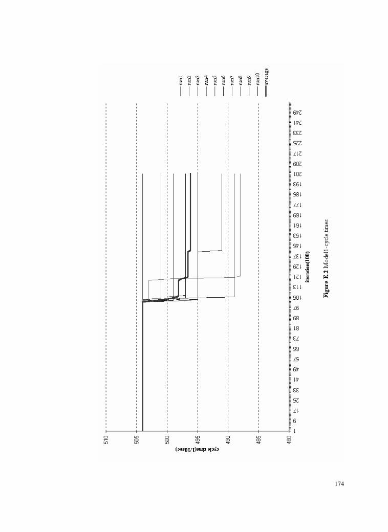
174

175

176

177
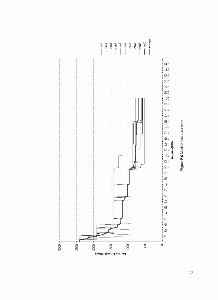
178

179

180
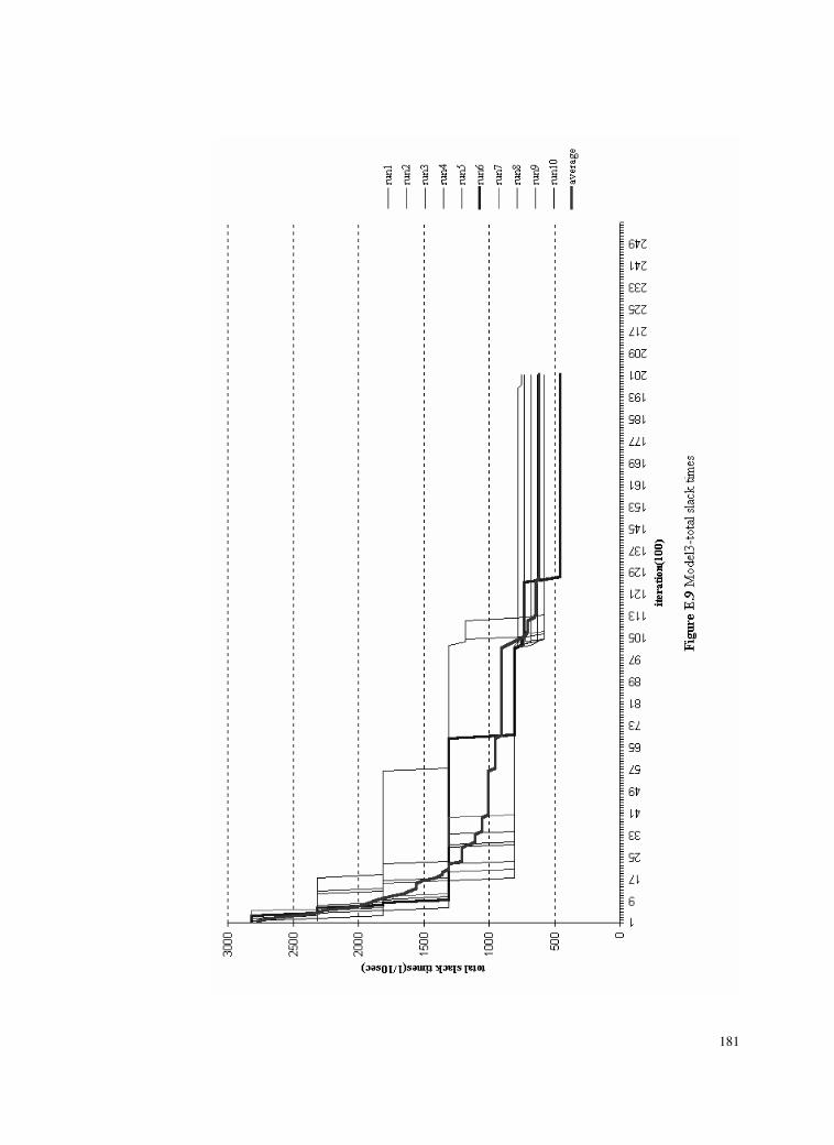
181
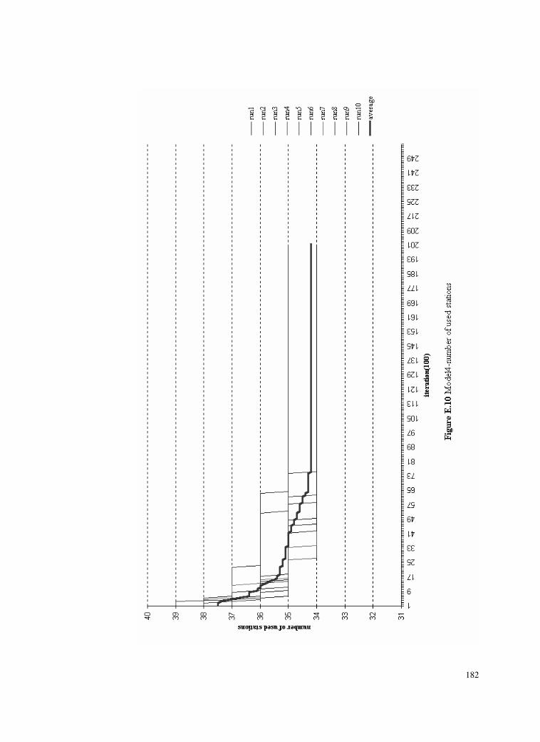
182
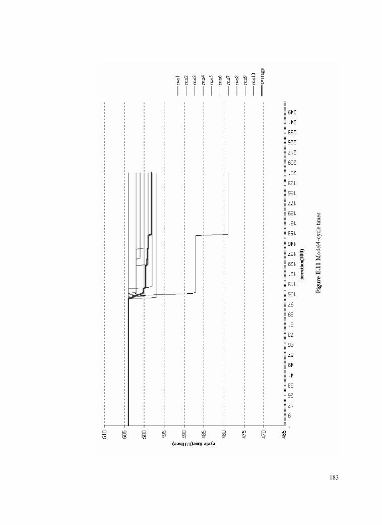
183

184
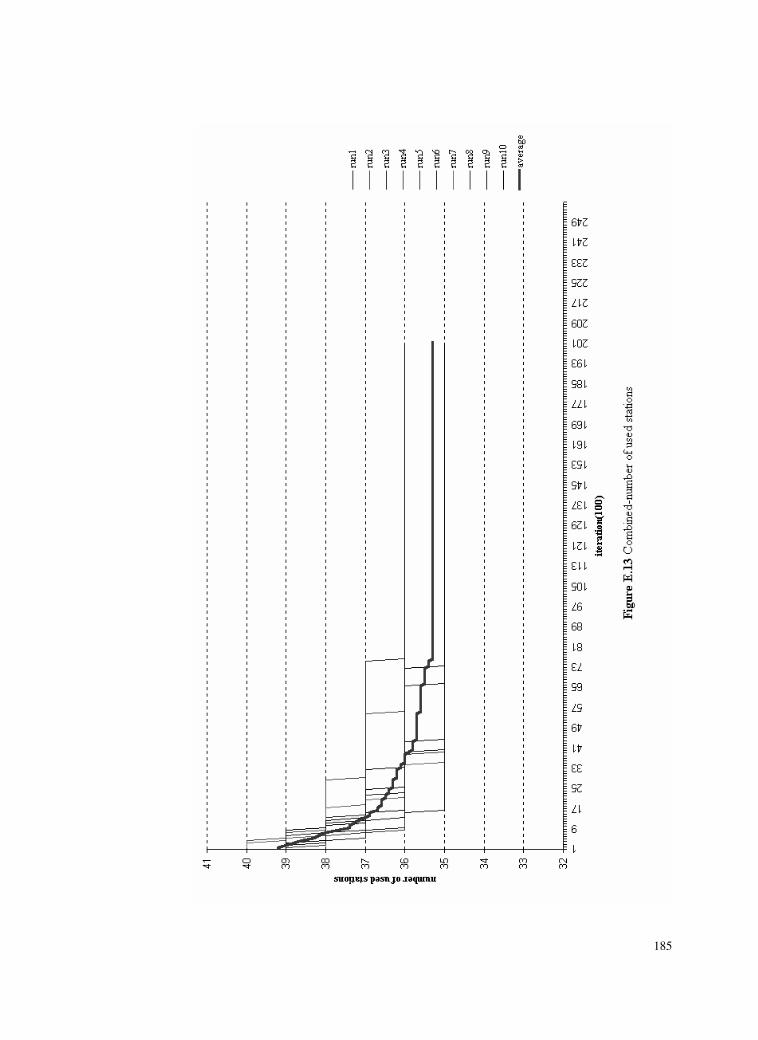
185

186

187
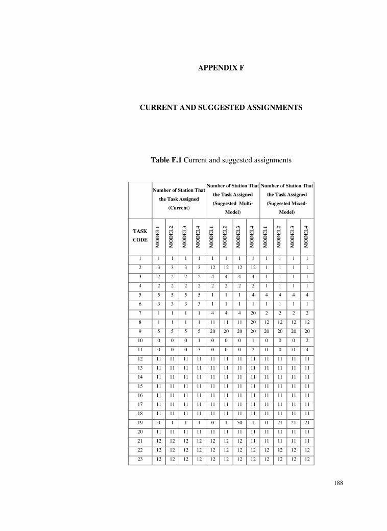
188
APPENDIX F
CURRENT AND SUGGESTED ASSIGNMENTS
Table F.1 Current and suggested assignments
Number of Station That
the Task Assigned
(Current)
Number of Station That
the Task Assigned
(Suggested Multi-
Model)
Number of Station That
the Task Assigned
(Suggested Mixed-
Model)
TASK
CODE
MO
DE
L1
MO
DE
L2
MO
DE
L3
MO
DE
L4
MO
DE
L1
MO
DE
L2
MO
DE
L3
MO
DE
L4
MO
DE
L1
MO
DE
L2
MO
DE
L3
MO
DE
L4
1 1 1 1 1 1 1 1 1 1 1 1 1
2 3 3 3 3 12 12 12 12 1 1 1 1
3 2 2 2 2 4 4 4 4 1 1 1 1
4 2 2 2 2 2 2 2 2 1 1 1 1
5 5 5 5 5 1 1 1 4 4 4 4 4
6 3 3 3 3 1 1 1 1 1 1 1 1
7 1 1 1 1 4 4 4 20 2 2 2 2
8 1 1 1 1 11 11 11 20 12 12 12 12
9 5 5 5 5 20 20 20 20 20 20 20 20
10 0 0 0 1 0 0 0 1 0 0 0 2
11 0 0 0 3 0 0 0 2 0 0 0 4
12 11 11 11 11 11 11 11 11 11 11 11 11
13 11 11 11 11 11 11 11 11 11 11 11 11
14 11 11 11 11 11 11 11 11 11 11 11 11
15 11 11 11 11 11 11 11 11 11 11 11 11
16 11 11 11 11 11 11 11 11 11 11 11 11
17 11 11 11 11 11 11 11 11 11 11 11 11
18 11 11 11 11 11 11 11 11 11 11 11 11
19 0 1 1 1 0 1 50 1 0 21 21 21
20 11 11 11 11 11 11 11 11 11 11 11 11
21 12 12 12 12 12 12 12 11 11 11 11 11
22 12 12 12 12 12 12 12 12 12 12 12 12
23 12 12 12 12 12 12 12 12 12 12 12 12
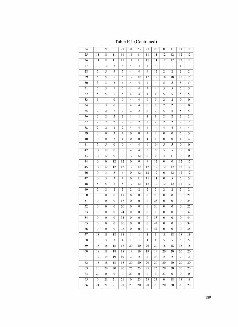
189
Table F.1 (Continued)
24 0 21 21 21 0 23 23 23 0 11 11 11
25 11 11 11 11 11 11 11 11 12 12 12 12
26 11 11 11 11 11 11 11 11 12 12 12 12
27 3 3 3 3 4 4 4 4 1 1 1 1
28 5 5 5 5 4 4 4 12 2 2 2 2
29 5 5 5 5 12 12 12 12 18 18 18 18
30 3 3 3 4 4 4 4 4 5 5 5 5
31 5 5 5 5 4 4 4 4 5 5 5 5
32 5 5 5 5 4 4 4 4 5 5 5 5
33 1 1 0 0 4 4 0 0 2 2 0 0
34 3 3 0 0 4 4 0 0 2 2 0 0
35 2 2 2 2 2 2 2 2 5 5 5 5
36 2 2 2 2 1 1 1 1 2 2 2 2
37 2 2 2 2 2 2 2 2 2 2 2 2
38 2 2 2 2 4 4 4 4 4 4 4 4
39 0 0 3 4 0 0 4 4 0 0 5 5
40 0 0 3 4 0 0 1 4 0 0 4 4
41 5 5 0 0 4 4 0 0 5 5 0 0
42 12 12 0 0 4 4 0 0 5 5 0 0
43 12 12 0 0 12 12 0 0 11 11 0 0
44 0 0 12 12 0 0 4 12 0 0 12 12
45 12 12 12 12 12 12 12 12 12 12 12 12
46 0 3 3 4 0 12 12 12 0 12 12 12
47 0 3 3 4 0 11 11 11 0 5 5 5
48 5 5 5 5 12 12 12 12 12 12 12 12
49 2 2 2 2 2 2 2 2 2 2 2 2
50 0 0 0 18 0 0 0 28 0 0 0 21
51 0 0 0 18 0 0 0 28 0 0 0 24
52 0 0 0 20 0 0 0 30 0 0 0 25
53 0 0 0 24 0 0 0 33 0 0 0 32
54 0 0 0 34 0 0 0 33 0 0 0 44
55 0 0 0 20 0 0 0 44 0 0 0 34
56 0 0 0 38 0 0 0 44 0 0 0 38
57 18 18 18 18 1 1 1 1 18 18 18 18
58 3 3 3 4 1 1 1 1 5 5 5 5
59 18 18 18 18 20 20 20 20 18 18 18 18
60 18 18 18 18 19 19 19 19 20 20 20 20
61 19 19 19 19 2 2 2 23 2 2 2 2
62 18 18 18 18 20 20 20 20 20 20 20 20
63 20 20 20 20 25 25 25 25 20 20 20 20
64 20 0 0 0 20 0 0 0 23 0 0 0
65 0 21 21 21 0 23 23 23 0 18 18 18
66 21 21 21 21 20 20 20 20 20 20 20 20

190
Table F.1 (Continued)
67 18 18 18 18 23 23 23 23 20 20 20 20
68 19 19 19 19 23 23 23 23 21 21 21 21
69 23 23 23 23 20 20 20 20 21 21 21 21
70 20 20 20 20 20 20 20 20 20 20 20 20
71 18 18 18 18 23 23 23 23 21 21 21 21
72 17 17 17 17 17 17 17 17 17 17 17 17
73 0 0 0 3 0 0 0 1 0 0 0 4
74 0 0 0 3 0 0 0 2 0 0 0 4
75 11 11 11 0 11 11 11 0 12 12 12 0
76 18 18 18 18 19 19 19 19 20 20 20 20
77 19 19 19 19 19 19 19 19 18 18 18 18
78 19 19 19 19 19 19 19 19 18 18 18 18
79 20 20 20 20 19 19 19 19 18 18 18 18
80 20 20 20 20 19 19 19 19 20 20 20 20
81 18 18 18 18 19 19 19 19 18 18 18 18
82 20 20 20 20 26 19 19 19 24 24 24 24
83 21 21 21 21 20 20 20 20 20 20 20 20
84 21 21 21 21 20 20 20 20 21 21 21 21
85 21 21 21 21 20 20 20 20 21 21 21 21
86 23 23 23 23 23 23 23 23 23 23 23 23
87 23 23 23 23 26 24 24 24 24 24 24 24
88 24 24 24 24 25 25 25 25 23 23 23 23
89 19 19 19 19 19 19 19 19 20 20 20 20
90 20 20 20 20 23 23 23 23 20 20 20 20
91 23 23 23 23 23 23 23 23 23 23 23 23
92 24 24 24 24 24 24 24 24 23 23 23 23
93 23 23 23 23 25 25 25 25 27 27 27 27
94 24 24 24 24 24 24 24 24 25 25 25 25
95 24 24 24 24 25 25 25 25 27 27 27 27
96 23 23 23 23 23 23 23 23 23 23 23 23
97 24 24 24 24 24 24 24 24 23 23 23 23
98 24 24 24 24 24 24 24 24 24 24 24 24
99 26 26 26 26 24 24 24 24 25 25 25 25
100 23 23 0 0 23 23 0 0 27 27 0 0
101 23 23 0 0 23 23 0 0 26 26 0 0
102 23 23 23 0 26 26 26 0 26 26 26 0
103 26 26 26 26 26 26 26 26 27 27 27 27
104 26 26 26 26 26 26 26 26 27 27 27 27
105 23 0 23 0 23 0 23 0 23 0 23 0
106 28 28 28 28 27 33 27 33 34 34 34 34
107 55 55 55 55 55 55 55 55 55 55 55 55
108 23 23 23 23 23 23 23 23 23 23 23 23
109 24 24 24 24 26 25 25 25 24 24 24 24
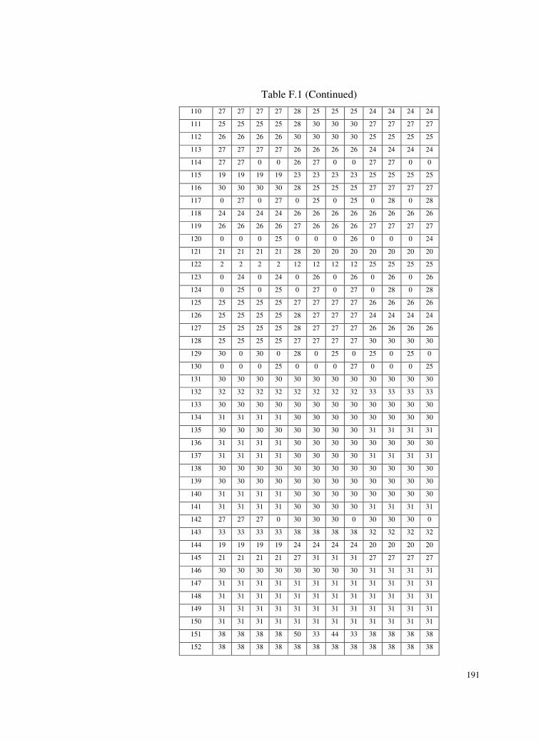
191
Table F.1 (Continued)
110 27 27 27 27 28 25 25 25 24 24 24 24
111 25 25 25 25 28 30 30 30 27 27 27 27
112 26 26 26 26 30 30 30 30 25 25 25 25
113 27 27 27 27 26 26 26 26 24 24 24 24
114 27 27 0 0 26 27 0 0 27 27 0 0
115 19 19 19 19 23 23 23 23 25 25 25 25
116 30 30 30 30 28 25 25 25 27 27 27 27
117 0 27 0 27 0 25 0 25 0 28 0 28
118 24 24 24 24 26 26 26 26 26 26 26 26
119 26 26 26 26 27 26 26 26 27 27 27 27
120 0 0 0 25 0 0 0 26 0 0 0 24
121 21 21 21 21 28 20 20 20 20 20 20 20
122 2 2 2 2 12 12 12 12 25 25 25 25
123 0 24 0 24 0 26 0 26 0 26 0 26
124 0 25 0 25 0 27 0 27 0 28 0 28
125 25 25 25 25 27 27 27 27 26 26 26 26
126 25 25 25 25 28 27 27 27 24 24 24 24
127 25 25 25 25 28 27 27 27 26 26 26 26
128 25 25 25 25 27 27 27 27 30 30 30 30
129 30 0 30 0 28 0 25 0 25 0 25 0
130 0 0 0 25 0 0 0 27 0 0 0 25
131 30 30 30 30 30 30 30 30 30 30 30 30
132 32 32 32 32 32 32 32 32 33 33 33 33
133 30 30 30 30 30 30 30 30 30 30 30 30
134 31 31 31 31 30 30 30 30 30 30 30 30
135 30 30 30 30 30 30 30 30 31 31 31 31
136 31 31 31 31 30 30 30 30 30 30 30 30
137 31 31 31 31 30 30 30 30 31 31 31 31
138 30 30 30 30 30 30 30 30 30 30 30 30
139 30 30 30 30 30 30 30 30 30 30 30 30
140 31 31 31 31 30 30 30 30 30 30 30 30
141 31 31 31 31 30 30 30 30 31 31 31 31
142 27 27 27 0 30 30 30 0 30 30 30 0
143 33 33 33 33 38 38 38 38 32 32 32 32
144 19 19 19 19 24 24 24 24 20 20 20 20
145 21 21 21 21 27 31 31 31 27 27 27 27
146 30 30 30 30 30 30 30 30 31 31 31 31
147 31 31 31 31 31 31 31 31 31 31 31 31
148 31 31 31 31 31 31 31 31 31 31 31 31
149 31 31 31 31 31 31 31 31 31 31 31 31
150 31 31 31 31 31 31 31 31 31 31 31 31
151 38 38 38 38 50 33 44 33 38 38 38 38
152 38 38 38 38 38 38 38 38 38 38 38 38
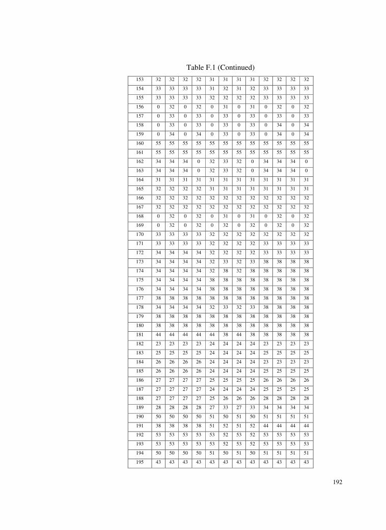
192
Table F.1 (Continued)
153 32 32 32 32 31 31 31 31 32 32 32 32
154 33 33 33 33 31 32 31 32 33 33 33 33
155 33 33 33 33 32 32 32 32 33 33 33 33
156 0 32 0 32 0 31 0 31 0 32 0 32
157 0 33 0 33 0 33 0 33 0 33 0 33
158 0 33 0 33 0 33 0 33 0 34 0 34
159 0 34 0 34 0 33 0 33 0 34 0 34
160 55 55 55 55 55 55 55 55 55 55 55 55
161 55 55 55 55 55 55 55 55 55 55 55 55
162 34 34 34 0 32 33 32 0 34 34 34 0
163 34 34 34 0 32 33 32 0 34 34 34 0
164 31 31 31 31 31 31 31 31 31 31 31 31
165 32 32 32 32 31 31 31 31 31 31 31 31
166 32 32 32 32 32 32 32 32 32 32 32 32
167 32 32 32 32 32 32 32 32 32 32 32 32
168 0 32 0 32 0 31 0 31 0 32 0 32
169 0 32 0 32 0 32 0 32 0 32 0 32
170 33 33 33 33 32 32 32 32 32 32 32 32
171 33 33 33 33 32 32 32 32 33 33 33 33
172 34 34 34 34 32 32 32 32 33 33 33 33
173 34 34 34 34 32 33 32 33 38 38 38 38
174 34 34 34 34 32 38 32 38 38 38 38 38
175 34 34 34 34 38 38 38 38 38 38 38 38
176 34 34 34 34 38 38 38 38 38 38 38 38
177 38 38 38 38 38 38 38 38 38 38 38 38
178 34 34 34 34 32 33 32 33 38 38 38 38
179 38 38 38 38 38 38 38 38 38 38 38 38
180 38 38 38 38 38 38 38 38 38 38 38 38
181 44 44 44 44 44 38 44 38 38 38 38 38
182 23 23 23 23 24 24 24 24 23 23 23 23
183 25 25 25 25 24 24 24 24 25 25 25 25
184 26 26 26 26 24 24 24 24 23 23 23 23
185 26 26 26 26 24 24 24 24 25 25 25 25
186 27 27 27 27 25 25 25 25 26 26 26 26
187 27 27 27 27 24 24 24 24 25 25 25 25
188 27 27 27 27 25 26 26 26 28 28 28 28
189 28 28 28 28 27 33 27 33 34 34 34 34
190 50 50 50 50 51 50 51 50 51 51 51 51
191 38 38 38 38 51 52 51 52 44 44 44 44
192 53 53 53 53 53 52 53 52 53 53 53 53
193 53 53 53 53 53 52 53 52 53 53 53 53
194 50 50 50 50 51 50 51 50 51 51 51 51
195 43 43 43 43 43 43 43 43 43 43 43 43
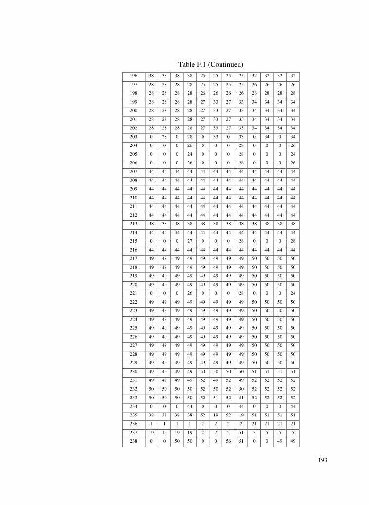
193
Table F.1 (Continued)
196 38 38 38 38 25 25 25 25 32 32 32 32
197 28 28 28 28 25 25 25 25 26 26 26 26
198 28 28 28 28 26 26 26 26 28 28 28 28
199 28 28 28 28 27 33 27 33 34 34 34 34
200 28 28 28 28 27 33 27 33 34 34 34 34
201 28 28 28 28 27 33 27 33 34 34 34 34
202 28 28 28 28 27 33 27 33 34 34 34 34
203 0 28 0 28 0 33 0 33 0 34 0 34
204 0 0 0 26 0 0 0 28 0 0 0 26
205 0 0 0 24 0 0 0 28 0 0 0 24
206 0 0 0 26 0 0 0 28 0 0 0 26
207 44 44 44 44 44 44 44 44 44 44 44 44
208 44 44 44 44 44 44 44 44 44 44 44 44
209 44 44 44 44 44 44 44 44 44 44 44 44
210 44 44 44 44 44 44 44 44 44 44 44 44
211 44 44 44 44 44 44 44 44 44 44 44 44
212 44 44 44 44 44 44 44 44 44 44 44 44
213 38 38 38 38 38 38 38 38 38 38 38 38
214 44 44 44 44 44 44 44 44 44 44 44 44
215 0 0 0 27 0 0 0 28 0 0 0 28
216 44 44 44 44 44 44 44 44 44 44 44 44
217 49 49 49 49 49 49 49 49 50 50 50 50
218 49 49 49 49 49 49 49 49 50 50 50 50
219 49 49 49 49 49 49 49 49 50 50 50 50
220 49 49 49 49 49 49 49 49 50 50 50 50
221 0 0 0 26 0 0 0 28 0 0 0 24
222 49 49 49 49 49 49 49 49 50 50 50 50
223 49 49 49 49 49 49 49 49 50 50 50 50
224 49 49 49 49 49 49 49 49 50 50 50 50
225 49 49 49 49 49 49 49 49 50 50 50 50
226 49 49 49 49 49 49 49 49 50 50 50 50
227 49 49 49 49 49 49 49 49 50 50 50 50
228 49 49 49 49 49 49 49 49 50 50 50 50
229 49 49 49 49 49 49 49 49 50 50 50 50
230 49 49 49 49 50 50 50 50 51 51 51 51
231 49 49 49 49 52 49 52 49 52 52 52 52
232 50 50 50 50 52 50 52 50 52 52 52 52
233 50 50 50 50 52 51 52 51 52 52 52 52
234 0 0 0 44 0 0 0 44 0 0 0 44
235 38 38 38 38 52 19 52 19 51 51 51 51
236 1 1 1 1 2 2 2 2 21 21 21 21
237 19 19 19 19 2 2 2 51 5 5 5 5
238 0 0 50 50 0 0 56 51 0 0 49 49

194
Table F.1 (Continued)
239 44 44 44 44 49 44 44 44 49 49 49 49
240 51 51 51 51 50 49 49 51 49 49 49 49
241 51 51 51 51 50 50 50 51 50 50 50 50
242 52 52 52 52 51 51 51 51 50 50 50 50
243 0 0 44 44 0 0 44 44 0 0 44 44
244 44 44 44 44 44 44 44 44 49 49 49 49
245 51 51 51 51 44 44 50 49 49 49 49 49
246 51 51 51 51 49 44 50 50 49 49 49 49
247 49 49 49 49 49 44 49 44 49 49 49 49
248 53 53 53 53 53 52 53 52 53 53 53 53
249 0 0 0 4 0 0 0 19 0 0 0 21
250 52 52 52 52 50 50 50 50 51 51 51 51
251 51 51 51 51 50 51 50 51 52 52 52 52
252 50 50 50 50 51 50 51 50 51 51 51 51
253 50 50 50 50 51 50 51 50 51 51 51 51
254 50 50 50 50 51 50 51 50 51 51 51 51
255 50 50 50 50 51 50 51 50 51 51 51 51
256 50 50 50 50 51 50 51 50 51 51 51 51
257 50 50 50 50 51 50 51 50 51 51 51 51
258 50 50 50 50 51 50 51 50 51 51 51 51
259 54 54 54 54 54 54 54 54 54 54 54 54
260 0 0 0 4 0 0 0 28 0 0 0 34
261 50 50 50 50 51 50 51 50 51 51 51 51
262 50 50 50 50 51 50 51 50 51 51 51 51
263 50 50 50 50 51 50 51 50 51 51 51 51
264 50 50 50 50 51 50 51 50 51 51 51 51
265 50 50 50 50 51 50 51 50 51 51 51 51
266 28 28 28 28 26 26 26 26 28 28 28 28
267 28 28 28 28 27 27 27 27 28 28 28 28
268 28 28 28 28 27 27 27 27 28 28 28 28
269 30 30 30 30 28 27 27 27 30 30 30 30
270 30 30 30 30 27 27 27 27 30 30 30 30
271 32 32 32 32 38 38 38 38 33 33 33 33
272 52 52 52 52 52 51 52 52 52 52 52 52
273 52 52 52 52 52 51 52 52 52 52 52 52
274 52 52 52 52 52 51 52 52 52 52 52 52
275 52 52 52 52 52 51 52 52 52 52 52 52
276 31 31 31 31 38 38 38 38 31 31 31 31
277 38 38 38 38 53 52 53 52 53 53 53 53
278 38 38 38 38 52 52 52 52 53 53 53 53
279 52 52 52 52 52 51 52 52 52 52 52 52
280 52 52 52 52 52 51 52 52 52 52 52 52
281 53 53 53 53 53 52 53 56 53 53 53 53
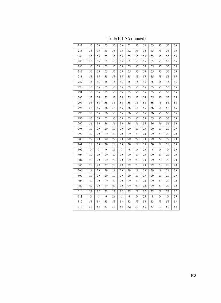
195
Table F.1 (Continued)
282 53 53 53 53 53 52 53 56 53 53 53 53
283 53 53 53 53 53 52 53 56 53 53 53 53
284 55 55 55 55 55 55 55 55 55 55 55 55
285 55 55 55 55 55 55 55 55 55 55 55 55
286 55 55 55 55 55 55 55 55 55 55 55 55
287 55 55 55 55 55 55 55 55 55 55 55 55
288 55 55 55 55 55 55 55 55 55 55 55 55
289 45 45 45 45 45 45 45 45 45 45 45 45
290 55 55 55 55 55 55 55 55 55 55 55 55
291 55 55 55 55 55 55 55 55 55 55 55 55
292 55 55 55 55 55 55 55 55 55 55 55 55
293 56 56 56 56 56 56 56 56 56 56 56 56
294 56 56 56 56 56 56 56 55 56 56 56 56
295 56 56 56 56 56 56 56 55 56 56 56 56
296 55 55 55 55 55 55 55 55 55 55 55 55
297 56 56 56 56 56 56 56 55 56 56 56 56
298 29 29 29 29 29 29 29 29 29 29 29 29
299 29 29 29 29 29 29 29 29 29 29 29 29
300 29 29 29 29 29 29 29 29 29 29 29 29
301 29 29 29 29 29 29 29 29 29 29 29 29
302 0 0 0 29 0 0 0 29 0 0 0 29
303 29 29 29 29 29 29 29 29 29 29 29 29
304 29 29 29 29 29 29 29 29 29 29 29 29
305 29 29 29 29 29 29 29 29 29 29 29 29
306 29 29 29 29 29 29 29 29 29 29 29 29
307 29 29 29 29 29 29 29 29 29 29 29 29
308 29 29 29 29 29 29 29 29 29 29 29 29
309 29 29 29 29 29 29 29 29 29 29 29 29
310 22 22 22 22 22 22 22 22 22 22 22 22
311 0 0 0 29 0 0 0 29 0 0 0 29
312 53 53 53 53 53 52 53 56 53 53 53 53
313 53 53 53 53 53 52 53 56 53 53 53 53