an adaptive scheduling algorithm for set cover problem in

Abstract—Redundant node deployment is a common strategy

in wireless sensor networks. This redundancy can be due to various reasons such as high probability of failures, long lifetime expectation, etc. One major problem in wireless sensor networks is to use this redundancy in order to extend the network lifetime while keeping the entire area under the coverage of the network. In this problem, which is known as set cover problem, the main objective is to select a subset of sensor nodes as active nodes so that the set of active nodes covers the entire area of the network. In this paper, an scheduling algorithm is presented for solving the set cover problem using cellular learning automata. In this algorithm, each node is equipped with a learning automaton which locally decides for the node to be active or not based on the situations of its neighbors. Simulation results in J-sim simulator environment specify the efficiency of the proposed scheduling algorithm over existing algorithms such as PEAS and PECAS.

Index Terms—Area coverage, cellular learning automata, learning automata, scheduling algorithm, wireless sensor networks.

I. INTRODUCTION One of the basic issues in wireless sensor networks is the

coverage problem which specifies how the network is monitored by sensor nodes [1]. The focus of this paper is on a sub-problem of coverage problem, called the set cover problem. In set cover problem, by assuming redundancy in the number of deployed sensor nodes throughout the area of the network, the main objective is to select a subset of sensor nodes as active nodes so that the set of active nodes covers the entire area of the network.

Selecting a subset of sensor nodes as active nodes is a suitable approach for prolonging the network lifetime. This is because in most scenarios of sensor networks, sensor nodes have limited batteries, which are not rechargeable. Hence, deactivating a number of sensor nodes which lets them conserve their batteries for later times, prolongs the lifetime of the network. Furthermore, deactivating some of the sensor nodes decreases the probability of collisions, which in turn, decreases the need for retransmitting packets. In this paper, we refer to any algorithm which can select a subset of sensor nodes in such a way that the entire area of the network is covered as scheduling algorithm.

Manuscript received May 14, 2012; revised August 14, 2012. R. Ghaderi is with the Computer Engineering Department, Islamic Azad

University, Arak 38135 Iran (e-mail: [email protected]). M. Esnaashari and M. R. Meybodi are with the Computer Engineering

and Information Technology Department, Amirkabir University of Technology, Tehran 15914 Iran (e-mail: [email protected]; [email protected]).

In this paper, a distributed, adaptive scheduling algorithm based on cellular learning automata for wireless sensor networks is proposed. The main purpose of this algorithm is to maintain coverage in the network with minimum number of active nodes, so that the total consumed energy of nodes is minimized. In the proposed algorithm, each node is equipped with a learning automaton which decides for the node to be active or not based on the states (either active or not) of its neighboring sensor nodes.

We used J-sim simulator to evaluate the performance of the proposed algorithm. Simulation results specify the efficiency of the proposed algorithm over existing algorithms such as PEAS [2] and PECAS [3] –especially against high ratio of unexpected failures.

The rest of this paper is organized as follows. In Section II, a literature overview is presented. In Section III, learning automata and cellular learning automata are briefly reviewed. The problem statement is given in Section IV. The proposed scheduling algorithm is described in Section V. Simulation results are given in Section VI. Section VII is the conclusion.

II. RELATED WORK Coverage problem is one of the basic issues in wireless

sensor network about which many distributed and centralized algorithms have been presented [2]–[7].

In [4], the problem of finding the maximal number of covers is paid attention to in which a cover is defined as a set of nodes that can completely cover the monitored area. This is an NP-complete problem which needs centralized heuristic solution. [5] pays attention to coverage problem in wireless sensor networks with a centralized manner. In this work, a genetic algorithm is used for coverage problem with the minimal number of nodes needed to cover entire area of the network.

In [6], [7], authors solve the coverage problem in a distributed manner. In this work, each node decides whether it can sleep or not based on the information collected from neighboring nodes.

In [2] a distributed, probing-based scheduling algorithm named PEAS is presented. In PEAS, a subset of nodes remains in active mode to maintain coverage and the rest of nodes go to sleep. Each sleeping node checks the existence of its working neighbor nodes after awakening. If no working node is within its probing range, it starts to operate in the active mode; otherwise, it returns to sleep state. PECAS algorithm [3] operates similar to PEAS, but unlike PEAS, in PECAS a node goes to sleep mode after a duration existing in working state and one of its neighboring nodes replaces with

An Adaptive Scheduling Algorithm for Set Cover Problem in Wireless Sensor Networks: A Cellular Learning

Automata Approach

Reza Ghaderi, Mehdi Esnaashari, and Mohammad Reza Meybodi

International Journal of Machine Learning and Computing, Vol. 2, No. 5, October 2012

62610.7763/IJMLC.2012.V2.203

it.

III. CELLULAR LEARNING AUTOMATA In this section, we briefly review learning automata and

cellular learning automata.

A. Learning Automata Learning Automata (LA) is an abstract model which

randomly selects one action out of its finite set of actions and performs it on a random environment. Environment then evaluates the selected action and responses to the automata with a reinforcement signal. Based on the selected action, and received signal, the automata updates its internal state and selects its next action. A class of LA is called variable structure learning automata and is represented by quadruple { }Tp,,,βα in which { }110 ,...,, −= rαααα represents the action set of the automata, { }110 ,...,, −= rββββ represents the input set, { }110 ,...,, −= rpppp represents the action probability set, and finally )](),(),([)1( npnnTnp βα=+ represents the learning algorithm. Let iα be the action chosen at time n . Then, the recurrence equation for updating p is defined as

ijjnpanpnpanpnp

jj

iii

≠∀−=+−+=+

,)()1()1()](1[)()1(

(1)

for favorable responses, and

ijjnpbr

bnp

npbnp

jj

ii

≠∀−+−

=+

−=+

,)()1(1

)1(

)()1()1(

(2)

for unfavorable ones. In these equations, a and b are reward and penalty parameters respectively. If ba = , learning algorithm is called PRL −

1; if ab << , it is called PRL ε2; and if

0=b , it is called IRL −3. For more information about learning

automata, the reader may refer to [8], [9]. B. Cellular Learning Automata Cellular Learning Automata (CLA), which is a

combination of Cellular Automata (CA) [10] and learning automata, is a powerful mathematical model for many decentralized problems and phenomena. The basic idea of CLA, which is a subclass of stochastic CA, is to utilize LA to adjust the state transition probability of stochastic CA. A CLA is a CA in which a learning automaton is assigned to every cell. The learning automaton residing in a particular cell determines its action (state) on the basis of its action probability vector. Like CA, there is a rule that the CLA operates under. The local rule of CLA and the actions selected by the neighboring LAs of any particular LA determine the reinforcement signal to the LA residing in a cell. CLA has found many applications such as image processing [11], rumor diffusion [12], channel assignment in cellular networks [13], and sensor networks [14], [15] to 1 Linear Reward-Penalty 2 Linear Reward epsilon Penalty 3 Linear Reward-Inaction

mention a few. For more information about CLA, the reader may refer to [12], [16].

IV. PROBLEM STATEMENT Consider a sensor network consists of N sensor nodes

Nsss ...,,, 21 within an area ( Ω ). Sensor nodes, which are responsible for sensing and monitoring the area, are scattered randomly throughout the area of the network so that Ω is completely covered. All sensor nodes have the same sensing range of sR and transmission range of tR . Each sensor node

is has 4 different modes of operation [17] as follows:

• On-duty ( AAA CSCPU ): CPU, sensing and communicating units are switched on referred to as active mode. A sensor node in the active mode is referred to as an active node.

• Sensing unit on-duty ( SAA CSCPU ): The CPU and the sensing units are switched on, but the communicating unit is switched off.

• Communicating unit on-duty ( ASA CSCPU ): The CPU and the communicating units are switched on, but the sensing unit is switched off.

• Off-duty ( SSS CSCPU ): CPU, sensing and communicating units are switched off referred to as sleep mode.

Note that in AAA CSCPU , SAA CSCPU , ASA CSCPU , and

SSS CSCPU , index A stands for active and index S stands for sleep. At any instance of time, a sensor node can be only in one of the above 4 operation modes.

We assume that the number of sensors ( N ) is greater than the one required to cover the entire area of the network. Thus, a scheduling algorithm can be adopted to use this redundancy for prolonging the lifetime of the network. Such a controlling algorithm, selects a subset of sensor nodes as active nodes so that the set of active nodes fully covers Ω .

Definition 1: Network lifetime is defined as the time elapsed from the network startup to the time at which Ω is not further completely covered by the network due to node deaths.

The above definitions and assumptions having been considered, the problem is to design a scheduling algorithm, which tries to maximize the lifetime of the network.

V. PROPOSED SCHEDULING ALGORITHM The proposed scheduling algorithm must provide two

requirements; 1. complete coverage of the network area, and 2. the set of the selected active nodes should consume as little power as possible so as to prolong the network lifetime. We consider the following assumptions:

• The set of sensor nodes residing throughout the network area covers the area completely.

• Sensor nodes are aware of their physical locations (using some localization techniques [18], [19]).

• N which is the number of sensor nodes within the area of the network is known by all nodes.


627


628

In what follows, we give the details of the proposed algorithm.

A. Detailed Description of the Proposed Scheduling Algorithm Initially, the network graph is mapped into a cellular

learning automaton. In this mapping, each sensor node is in the network is mapped into a cell i in CLA, and two cells iand j are adjacent in CLA if their corresponding sensor nodes are located within the sensing ranges of each other, or in other words, two cells are adjacent if the distance between their corresponding sensor nodes is not more than nR given by following equation:

ssn RRR 22 ≅−= ε (3)

We refer to nR as neighborhood radius hereafter. The learning automaton in each cell i of CLA, referred to

as iLA uses linear learning algorithm given by (1) and (2). All learning automata are PRL − . Each iLA has two actions 0αand 1α ; 0α is "plan to be in active mode", and 1α is "plan to be in sleep mode". The probability of selecting each of these actions is initially computed according to (4).

01

0

1 ppNNp I

−=

=

(4)

In this equation, IN is a constant which is greater than the minimum number of active nodes required to cover the entire area of the network. 0p is selected this way in order to have a suitable initial distribution (in terms of area coverage) of active nodes throughout the network area.

Neighboring nodes exchange HELLO packets with each other periodically to be aware of the states of each other. Details on how to compute the time interval between two consecutive transmissions of HELLO packets in each sensor node will be given in Subsection V-A-1. The HELLO packet of a node contains its id and physical location. Using received HELLO packets, each sensor node is stores for any of its active neighboring nodes, the location and the time of the last received HELLO packet.

Sensor nodes are initially in “INITIAL” state. In this state, all nodes are in SSS CSCPU operation mode. Each node isawakes after a random duration which is selected uniformly from the range ),0( 0τ . 0τ is the maximum allowed time interval between two subsequent transmissions of HELLO packets. When a node is awakes, it uses its learning automaton to choose its state. If iLA selects 0α which is "plan to be in active mode", sensor node is changes its operation mode from SSS CSCPU to AAA CSCPU and its state from “INITIAL” to “WORK” and then, broadcasts a HELLO packet in its neighborhood. If iLA selects 1α which is "plan to be in sleep mode", is changes its operation mode

to ASA CSCPU and its state to “WAIT_FOR_SLEEP”, and then, waits to receive HELLO packets from its neighbors which are in “WORK” state. A node which is in “WORK” state (referred to as a working node) monitors its surrounding area, and broadcasts HELLO packets to its neighboring nodes periodically.

The reinforcement signal is computed according to the following two cases:

• If is is in “WORK” state and its received HELLO packets within 0τ duration guarantee that the monitored area of is is covered by its neighbors, then it penalizes its selected action. Otherwise, it rewards its selected action.

• If is is in “WAIT_FOR_SLEEP” state and its received HELLO packets within 0τ duration, do not guarantee that the monitored area of is is covered by its neighbors, then it penalizes its selected action. Otherwise, isrewards its selected action.

Each working sensor node guarantees not to change its state for a predetermined duration T starting from the time it dispatches its HELLO packet. As a result, if a node, which is in “WAIT_FOR_SLEEP” state, is ensured (through received HELLO packets) that its monitored area is covered completely by its active neighboring nodes within 0τduration, then it switches to “SLEEP” state. In “SLEEP” state, all nodes are in SSS CSCPU operation mode. Sleeping time is determined by considering the value of T and the receipt times of the last HELLO packets from active neighbors. Let t be the current time of the network and R

it be the receipt time of the last HELLO packet from active neighbor is at

node js . The sleeping time of the node js ( sleepjT ) is then

computed according to the following equation:

( ))(min Risofneighborsactives

sleepj ttTT

ji

−−=∈ (5)

When the sleeping time of the node is is over, node ischanges its operation mode to ASA CSCPU and its state to “WAIT_FOR_SLEEP”.

Next time for action selection of the learning automaton of a node is is determined as follows:

• If node is is in “WAIT_FOR_SLEEP” state and action

1α is penalized, next action selection time is immediately after receiving the environment response.

• If node is is in “WORK” state and action 0α is penalized, next action selection time is at the dispatching time of the next HELLO packet. If the selected action of such a node is 1α , then is enters “WAIT_FOR_SLEEP" state, but due to the assurance of this node to its neighbors, is must stay in active mode and perform all of the tasks of a sensor node in “WORK” state, except for sending HELLO packets, until the end of the assurance time.

• If the selected action of node is is rewarded, then the

next action selection time is when this action is penalized. In other words, the rewarded action is performed repeatedly until the time it receives penalty.

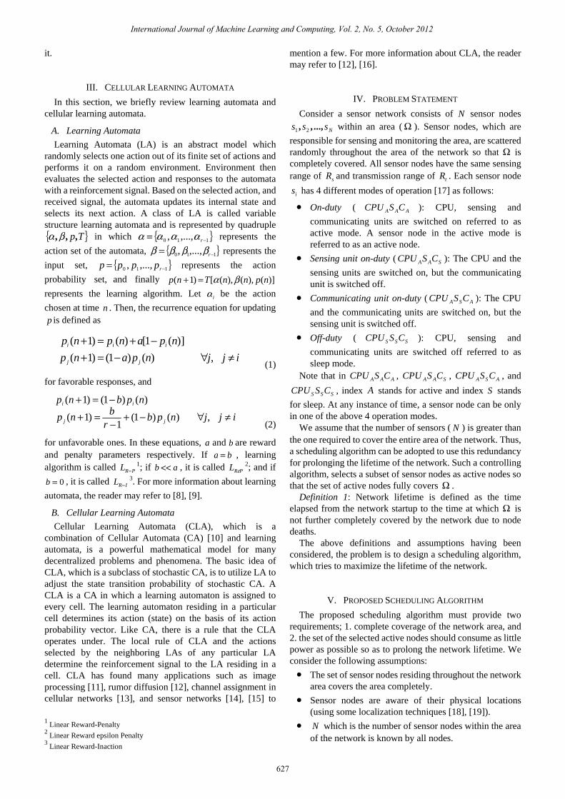
In Fig. 1, the transition diagram of operation mode / state of the proposed scheduling algorithm in each sensor node has been shown. Fig. 2 shows the pseudo code of the proposed algorithm.

Fig. 1. Operation mode / State transition diagram of the proposed scheduling

algorithm in each sensor node.

1) Time Interval for Transmission of HELLO Packets

As we stated before, sensor nodes which are in “WORK” state, periodically broadcast HELLO packets. Initially, the time interval between two consecutive transmissions of HELLO packets for each sensor node is is set to 0ττ =i . Immediately after sending the k th ( 1>k ) HELLO packet, each node is updates iτ according to (6).

⎪⎩

⎪⎨

⎧

×

==

OtherwiseNNo

No

I

i

i

i ;

0;

0

0

τ

ττ

(6)

In the above equation, iNo is the number of working nodes from which is receives at least one HELLO packet within the time interval ],[ 0 tt τ− . Since iNo is a measure of the traffic load in the neighborhood of is , (6) makes the time interval between two consecutive transmissions of HELLO packets in each sensor node adaptable to the local traffic load in the neighborhood of that node.

VI. PERFORMANCE EVALUATION

A. Simulation Setup To evaluate the performance of the proposed scheduling

algorithm, we conduct a number of experiments. The results obtained from the proposed algorithm are compared with the results obtained from PEAS [2] and PECAS [3]. Experiments are simulated using J-sim simulator [20]. We use a network area of 50m×50m through which a number of sensor nodes are scattered uniformly at random.

Energy model given in [7] is used in which the energy consumption ratios for transmission, reception (idle) and sleep modes are 20:4:0.01 respectively. The initial energy level of each sensor node is chosen randomly from the range of 28 to 35 Jules. Sensing and transmission ranges of each sensor node are 17m and 30m, respectively. Therefore, neighborhood radius according to (3) is 34m. Like PEAS [2], each node has a raw wireless communication capacity of 20Kbps. Simulation time for the first two experiments is assumed to be 1000s. Results are averaged over 25 runs of simulations. 1) Parameters of the Proposed Algorithm

We consider the value of parameter T as 10s and rate of reward and penalty parameters as 0.75 so that the sensor nodes have rapid reactions to topology changes of the network (due to unexpected failures, energy exhaustion of sensor nodes, ...). The values for the parameters in the proposed algorithm are listed in Table I.

TABLE I: PARAMETER VALUES USED IN THE PROPOSED ALGORITHM

2) Evaluation Metrics

To evaluate the performance of the proposed algorithm, we use the following metrics: (i) number of active nodes; (ii) percentage of area under the coverage of the network; (iii) total consumed energy of sensor nodes; and (iv) network lifetime.

B. Simulation Results 1) Experiment 1

This experiment is conducted to study the performance of the proposed algorithm in terms of number of active nodes, percentage of area under the coverage of the network, and

sR tR IN Initial energy of each sensor node

Channel capacity

T 0τ ba,

17m 30m 25 28 to 35 Jules 20Kbps 10s 1.27s 0.75


629

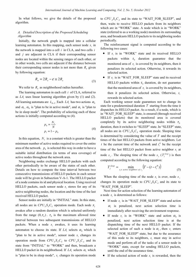
Fig. 2. Pseudo code of the proposed algorithm

For each node is corresponding with cell i in CLA do in parallel Initialize WakeupAfter(Random ),0( 0τ ) Select an action according to (4) If (the action is 0α ) then

ChangeOperation_Mode/StateTo( AAA CSCPU / “WORK”)

else /* the action is 1α */

ChangeOperation_Mode/StateTo( ASA CSCPU / “WAIT_FOR_SLEEP”) End if While (Not SensorDead) do While (the node is in “WORK” State) do Broadcast HELLO Packet Update LA’s probability vector End while While (the node is in “WAIT_FOR_SLEEP” State) do If (NOT AssuranceToNeighbors) then If (monitored area of the node is covered by neighbors) then ChangeOperation_Mode/StateTo( SSS CSCPU / “SLEEP”) End if End if Update LA’s probability vector End while If (the node is in “SLEEP” State) then WakeupAfter(SleepingTime) ChangeOperation_Mode/StateTo( ASA CSCPU / “WAIT_FOR_SLEEP”) End if End While End for

total consumed energy of sensor nodes in comparison to PEAS and PECAS algorithms. Experiment is repeated for 50, 100, 200, 400, and 500 sensor nodes.

Fig. 3 shows the results of the comparison for the ‘number of active nodes’ metric. It can be seen from this figure that the number of active nodes in the proposed algorithm, unlike PEAS and PECAS algorithms, does not depend heavily on the number of sensor nodes in the network.

Fig. 3. Number of active nodes versus number of sensor nodes

Fig. 4. Percent of coverage versus number of sensor nodes

Fig. 4 presents the results of the comparison between the

proposed algorithm, PEAS, and PECAS in terms of percentage of network area under coverage. As it can be seen from the figure, the proposed algorithm fully covers the network area even in the networks of small sizes (networks in which the number of sensor nodes is below 100). Fig. 5 compares the proposed algorithm with PEAS and PECAS algorithms in terms of the total energy consumption of sensor nodes. It can be seen from this figure that the proposed algorithm consumes less than 70% and 45% of the energy consumed by PEAS and PECAS, respectively. 2) Experiment 2

In this experiment, we study the tolerability of the proposed algorithm against unexpected failures of sensor nodes in comparison to PEAS and PECAS algorithms. To simulate unexpected failures of sensor nodes, in this experiment, 50% of the sensor nodes experience failures in random times during the operation of the network. Similar to

Experiment 1, networks with 50, 100, 200, 400, and 500 sensor nodes are considered for this experiment.

Fig. 5. Total energy consumption versus number of sensor nodes

Fig. 6. Number of active nodes versus number of sensor nodes with failures

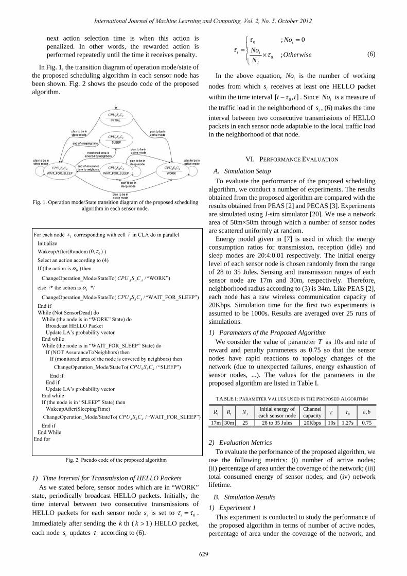
Fig. 6, which compares the proposed algorithm with PEAS and PECAS in terms of average number of active nodes, indicates that the presence of failures does not affect the performance of the proposed algorithm in terms of this metric significantly. Number of active nodes in the proposed algorithm is less than 49% and 40% of the number of active nodes in PEAS and PECAS algorithms respectively. According to Fig. 7, which gives the comparison of the mentioned algorithms in terms of percentage of network area under coverage, the proposed algorithm provides full coverage of network area in all of mentioned network sizes even in presence of unexpected node failures.

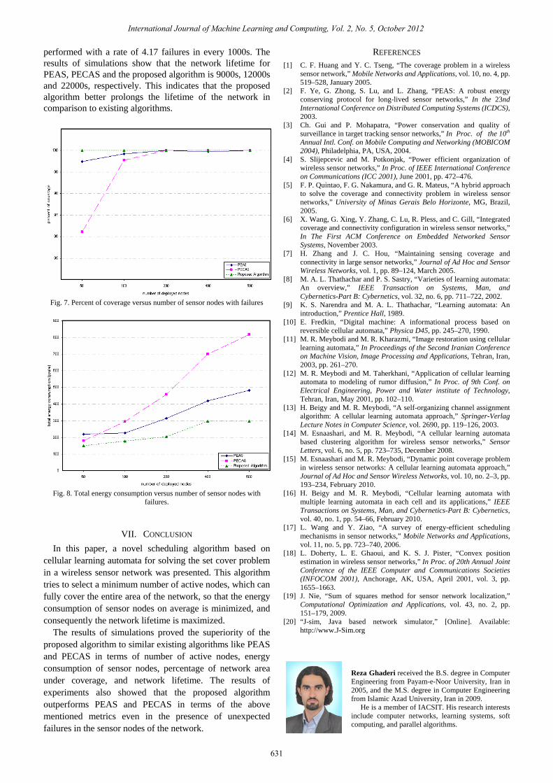
Finally, Fig. 8 gives the comparison of the mentioned algorithms in terms of the total energy consumption of sensor nodes. This figure shows that in the presence of unexpected failures, the energy consumption of the proposed algorithm is less than 69% and 54% of the energy consumption of PEAS and PECAS, respectively.

3) Experiment 3 This experiment is conducted to study the performance of

the proposed algorithm in terms of network lifetime. For this experiment, number of sensor nodes is assumed to be 250. The injection of unexpected failures of sensor nodes is


630

performed with a rate of 4.17 failures in every 1000s. The results of simulations show that the network lifetime for PEAS, PECAS and the proposed algorithm is 9000s, 12000s and 22000s, respectively. This indicates that the proposed algorithm better prolongs the lifetime of the network in comparison to existing algorithms.

Fig. 7. Percent of coverage versus number of sensor nodes with failures

Fig. 8. Total energy consumption versus number of sensor nodes with

failures.

VII. CONCLUSION In this paper, a novel scheduling algorithm based on

cellular learning automata for solving the set cover problem in a wireless sensor network was presented. This algorithm tries to select a minimum number of active nodes, which can fully cover the entire area of the network, so that the energy consumption of sensor nodes on average is minimized, and consequently the network lifetime is maximized.

The results of simulations proved the superiority of the proposed algorithm to similar existing algorithms like PEAS and PECAS in terms of number of active nodes, energy consumption of sensor nodes, percentage of network area under coverage, and network lifetime. The results of experiments also showed that the proposed algorithm outperforms PEAS and PECAS in terms of the above mentioned metrics even in the presence of unexpected failures in the sensor nodes of the network.

REFERENCES [1] C. F. Huang and Y. C. Tseng, “The coverage problem in a wireless

sensor network,” Mobile Networks and Applications, vol. 10, no. 4, pp. 519–528, January 2005.

[2] F. Ye, G. Zhong, S. Lu, and L. Zhang, “PEAS: A robust energy conserving protocol for long-lived sensor networks,” In the 23nd International Conference on Distributed Computing Systems (ICDCS), 2003.

[3] Ch. Gui and P. Mohapatra, “Power conservation and quality of surveillance in target tracking sensor networks,” In Proc. of the 10th Annual Intl. Conf. on Mobile Computing and Networking (MOBICOM 2004), Philadelphia, PA, USA, 2004.

[4] S. Slijepcevic and M. Potkonjak, “Power efficient organization of wireless sensor networks,” In Proc. of IEEE International Conference on Communications (ICC 2001), June 2001, pp. 472–476.

[5] F. P. Quintao, F. G. Nakamura, and G. R. Mateus, “A hybrid approach to solve the coverage and connectivity problem in wireless sensor networks,” University of Minas Gerais Belo Horizonte, MG, Brazil, 2005.

[6] X. Wang, G. Xing, Y. Zhang, C. Lu, R. Pless, and C. Gill, “Integrated coverage and connectivity configuration in wireless sensor networks,” In The First ACM Conference on Embedded Networked Sensor Systems, November 2003.

[7] H. Zhang and J. C. Hou, “Maintaining sensing coverage and connectivity in large sensor networks,” Journal of Ad Hoc and Sensor Wireless Networks, vol. 1, pp. 89–124, March 2005.

[8] M. A. L. Thathachar and P. S. Sastry, “Varieties of learning automata: An overview,” IEEE Transaction on Systems, Man, and Cybernetics-Part B: Cybernetics, vol. 32, no. 6, pp. 711–722, 2002.

[9] K. S. Narendra and M. A. L. Thathachar, “Learning automata: An introduction,” Prentice Hall, 1989.

[10] E. Fredkin, “Digital machine: A informational process based on reversible cellular automata,” Physica D45, pp. 245–270, 1990.

[11] M. R. Meybodi and M. R. Kharazmi, “Image restoration using cellular learning automata,” In Proceedings of the Second Iranian Conference on Machine Vision, Image Processing and Applications, Tehran, Iran, 2003, pp. 261–270.

[12] M. R. Meybodi and M. Taherkhani, “Application of cellular learning automata to modeling of rumor diffusion,” In Proc. of 9th Conf. on Electrical Engineering, Power and Water institute of Technology, Tehran, Iran, May 2001, pp. 102–110.

[13] H. Beigy and M. R. Meybodi, “A self-organizing channel assignment algorithm: A cellular learning automata approach,” Springer-Verlag Lecture Notes in Computer Science, vol. 2690, pp. 119–126, 2003.

[14] M. Esnaashari, and M. R. Meybodi, “A cellular learning automata based clustering algorithm for wireless sensor networks,” Sensor Letters, vol. 6, no. 5, pp. 723–735, December 2008.

[15] M. Esnaashari and M. R. Meybodi, “Dynamic point coverage problem in wireless sensor networks: A cellular learning automata approach,” Journal of Ad Hoc and Sensor Wireless Networks, vol. 10, no. 2–3, pp. 193–234, February 2010.

[16] H. Beigy and M. R. Meybodi, “Cellular learning automata with multiple learning automata in each cell and its applications,” IEEE Transactions on Systems, Man, and Cybernetics-Part B: Cybernetics, vol. 40, no. 1, pp. 54–66, February 2010.

[17] L. Wang and Y. Ziao, “A survey of energy-efficient scheduling mechanisms in sensor networks,” Mobile Networks and Applications, vol. 11, no. 5, pp. 723–740, 2006.

[18] L. Doherty, L. E. Ghaoui, and K. S. J. Pister, “Convex position estimation in wireless sensor networks,” In Proc. of 20th Annual Joint Conference of the IEEE Computer and Communications Societies (INFOCOM 2001), Anchorage, AK, USA, April 2001, vol. 3, pp. 1655–1663.

[19] J. Nie, “Sum of squares method for sensor network localization,” Computational Optimization and Applications, vol. 43, no. 2, pp. 151–179, 2009.

[20] “J-sim, Java based network simulator,” [Online]. Available: http://www.J-Sim.org

Reza Ghaderi received the B.S. degree in Computer Engineering from Payam-e-Noor University, Iran in 2005, and the M.S. degree in Computer Engineering from Islamic Azad University, Iran in 2009. He is a member of IACSIT. His research interests include computer networks, learning systems, soft computing, and parallel algorithms.


631

Mehdi Esnaashari received the B.S., M.S., and Ph.D. degrees in Computer Engineering from Amirkabir University of Technology, Iran in 2002, 2005, and 2011, respectively. His research interests include computer networks, learning systems, and soft computing.

Mohammad Reza Meybodi received the B.S. and M.S. degrees in Economics from Shahid Beheshti University, Iran in 1973 and 1977, respectively. He also received the M.S. and Ph.D. degrees from Oklahoma University, USA in 1980 and 1983, respectively, in Computer Science. Currently, he is a Full Professor in Computer Engineering and Information Technology Department, Amirkabir University of Technology, Tehran, Iran. Prior to

current position, he worked from 1983 to 1985 as an Assistant Professor at Western Michigan University, and from 1985 to 1991 as an Associate Professor at Ohio University, USA. His research interests include channel management in cellular networks, learning systems, parallel algorithms, soft computing, and software development.


632

an adaptive scheduling algorithm for set cover problem in

Documents