An Adaptive Algorithm for Dealing withSparse Multidimensional Data Sets

Presented to

Department of Statistics

October 18, 2004

Prof. Andrew MeadeDept. MEMS

Presentation Outline

•Background

• Approach

• Performance

•Applications

•Conclusions/Future Work

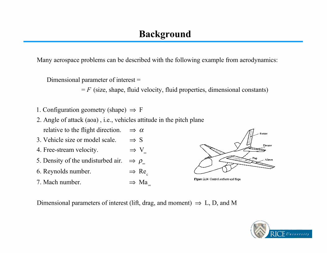
Many aerospace problems can be described with the following example from aerodynamics:

Dimensional parameter of interest =

= F (size, shape, fluid velocity, fluid properties, dimensional constants)

1. Configuration geometry (shape) ⇒ F

2. Angle of attack (aoa) , i.e., vehicles attitude in the pitch plane

relative to the flight direction. ⇒ α3. Vehicle size or model scale. ⇒ S

4. Free-stream velocity. ⇒ V∞

5. Density of the undisturbed air. ⇒ ρ∞

6. Reynolds number. ⇒ Rec

7. Mach number. ⇒ Ma∞

Dimensional parameters of interest (lift, drag, and moment) ⇒ L, D, and M

Background

We define the dynamic pressure as q∞ = 1

2ρ∞V∞

2 ,

the Reynolds number based on the chord as Rec =

ρ∞V∞c

µ∞

,

the freestream Mach number as Ma∞ =V∞

a∞

,

and the reference area (planform area) as S = bc .

Background

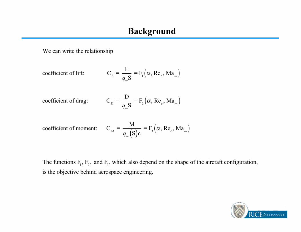
We can write the relationship

coefficient of lift: CL =

L

q∞S = F

1α , Re

c, Ma∞( )

coefficient of drag: CD

= D

q∞S = F

2α , Re

c, Ma∞( )

coefficient of moment: CM

= M

q∞ S( )c = F3α , Re

c, Ma∞( )

The functions F1, F

2, and F

3, which also depend on the shape of the aircraft configuration,

is the objective behind aerospace engineering.

Background

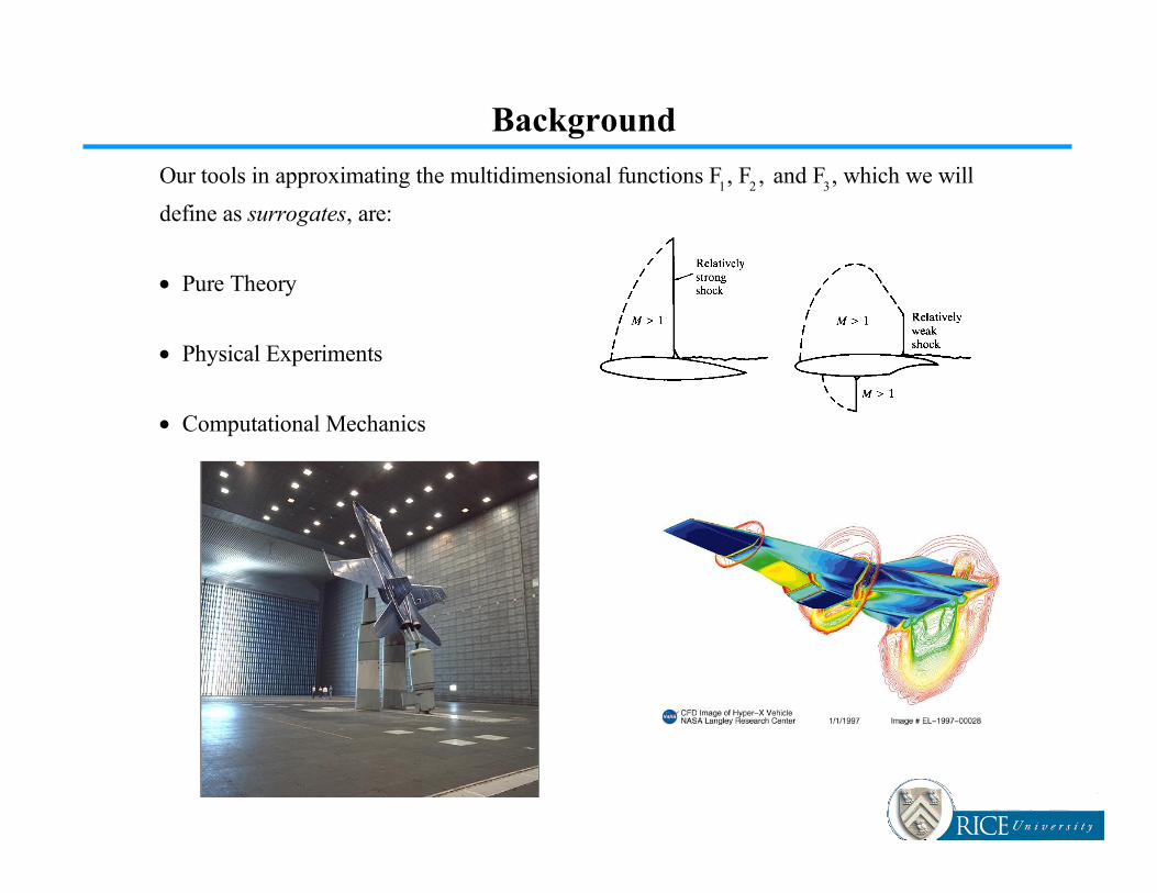
Our tools in approximating the multidimensional functions F1, F

2, and F

3, which we will

define as surrogates, are:

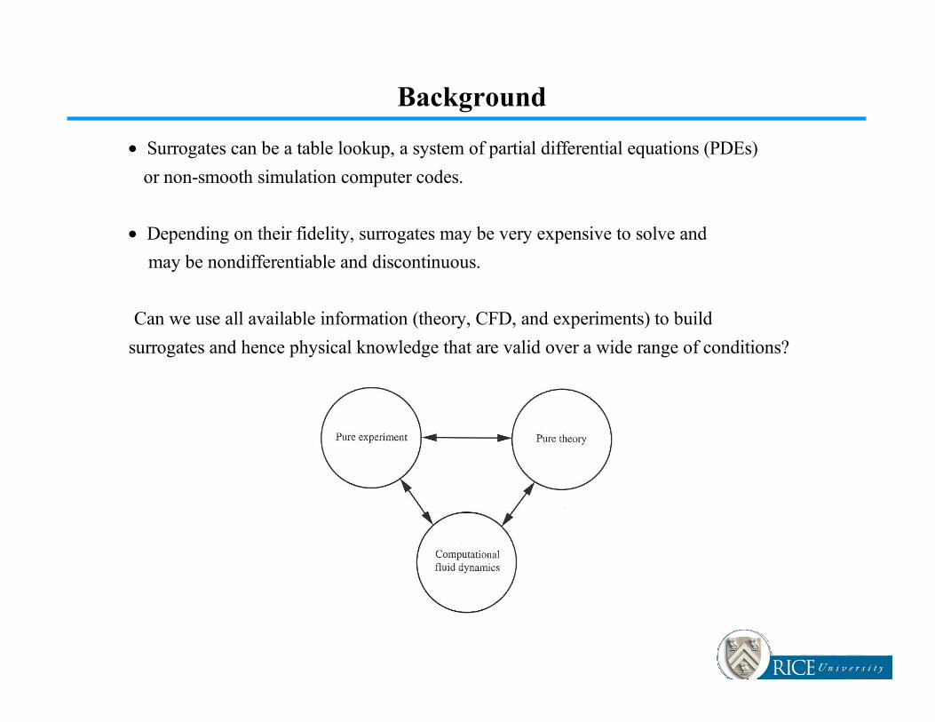
• Pure Theory

• Physical Experiments

• Computational Mechanics

Background

Background

• Surrogates can be a table lookup, a system of partial differential equations (PDEs)

or non-smooth simulation computer codes.

• Depending on their fidelity, surrogates may be very expensive to solve and

may be nondifferentiable and discontinuous.

Can we use all available information (theory, CFD, and experiments) to build

surrogates and hence physical knowledge that are valid over a wide range of conditions?

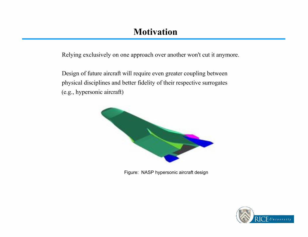
Figure: NASP hypersonic aircraft design

Motivation

Relying exclusively on one approach over another won't cut it anymore.

Design of future aircraft will require even greater coupling between

physical disciplines and better fidelity of their respective surrogates

(e.g., hypersonic aircraft)

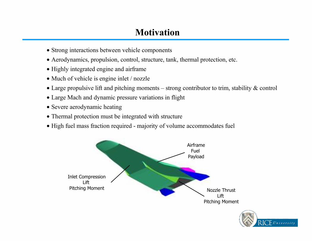
Inlet CompressionLift

Pitching Moment Nozzle ThrustLift

Pitching Moment

AirframeFuel

Payload

Motivation

• Strong interactions between vehicle components

• Aerodynamics, propulsion, control, structure, tank, thermal protection, etc.

• Highly integrated engine and airframe

• Much of vehicle is engine inlet / nozzle

• Large propulsive lift and pitching moments – strong contributor to trim, stability & control

• Large Mach and dynamic pressure variations in flight

• Severe aerodynamic heating

• Thermal protection must be integrated with structure

• High fuel mass fraction required - majority of volume accommodates fuel

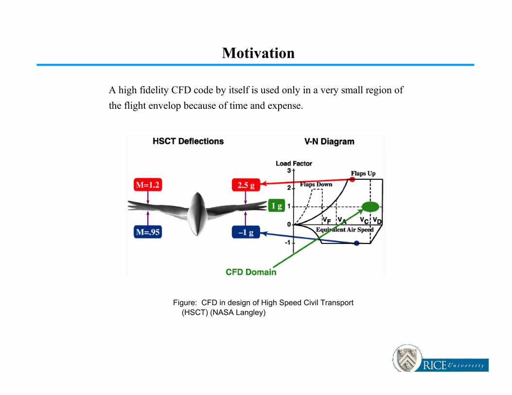
Figure: CFD in design of High Speed Civil Transport(HSCT) (NASA Langley)

A high fidelity CFD code by itself is used only in a very small region of

the flight envelop because of time and expense.

Motivation

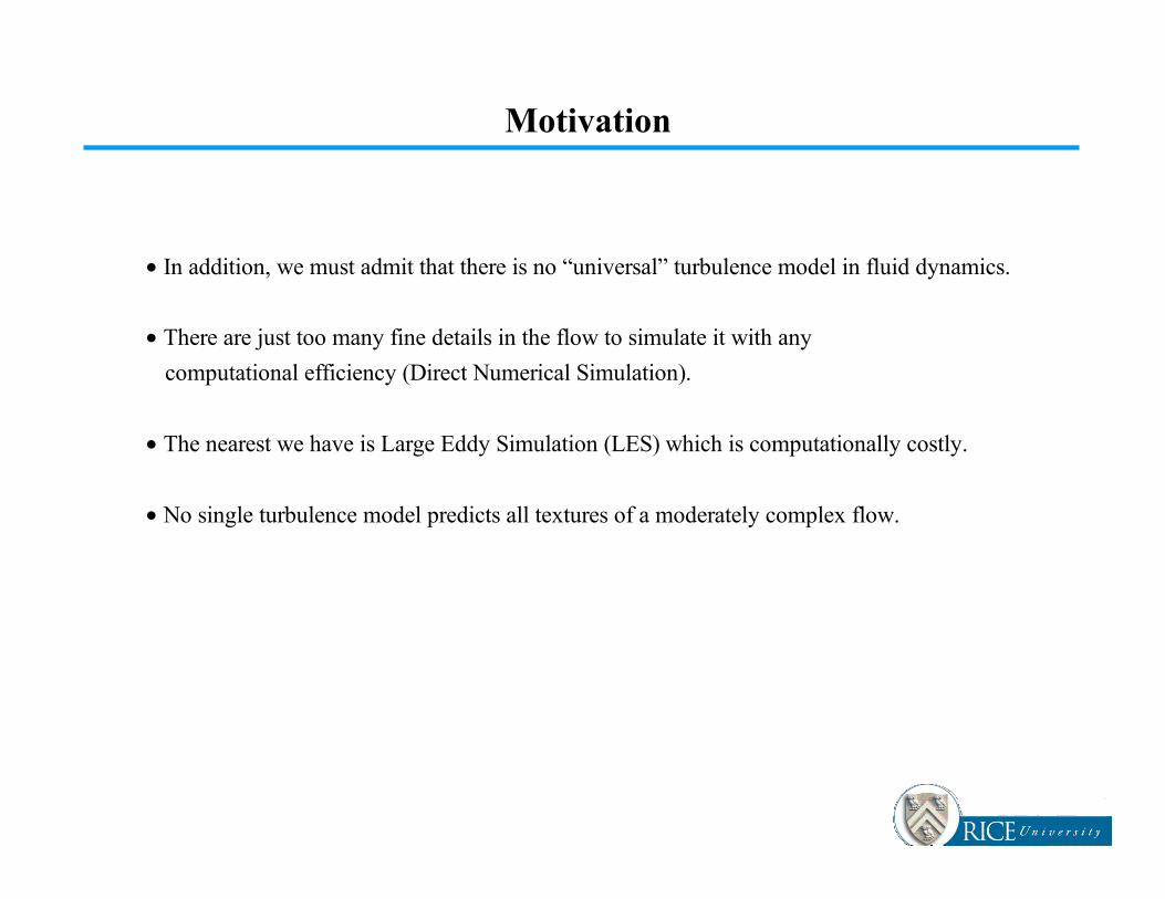
• In addition, we must admit that there is no “universal” turbulence model in fluid dynamics.

• There are just too many fine details in the flow to simulate it with any

computational efficiency (Direct Numerical Simulation).

• The nearest we have is Large Eddy Simulation (LES) which is computationally costly.

• No single turbulence model predicts all textures of a moderately complex flow.

Motivation

Motivation

Figure: Hemsch wing-body-nacelle wind tunnelmodel for the AIAA Drag Prediction Workshop(NASA Langley)

Motivation

Motivation

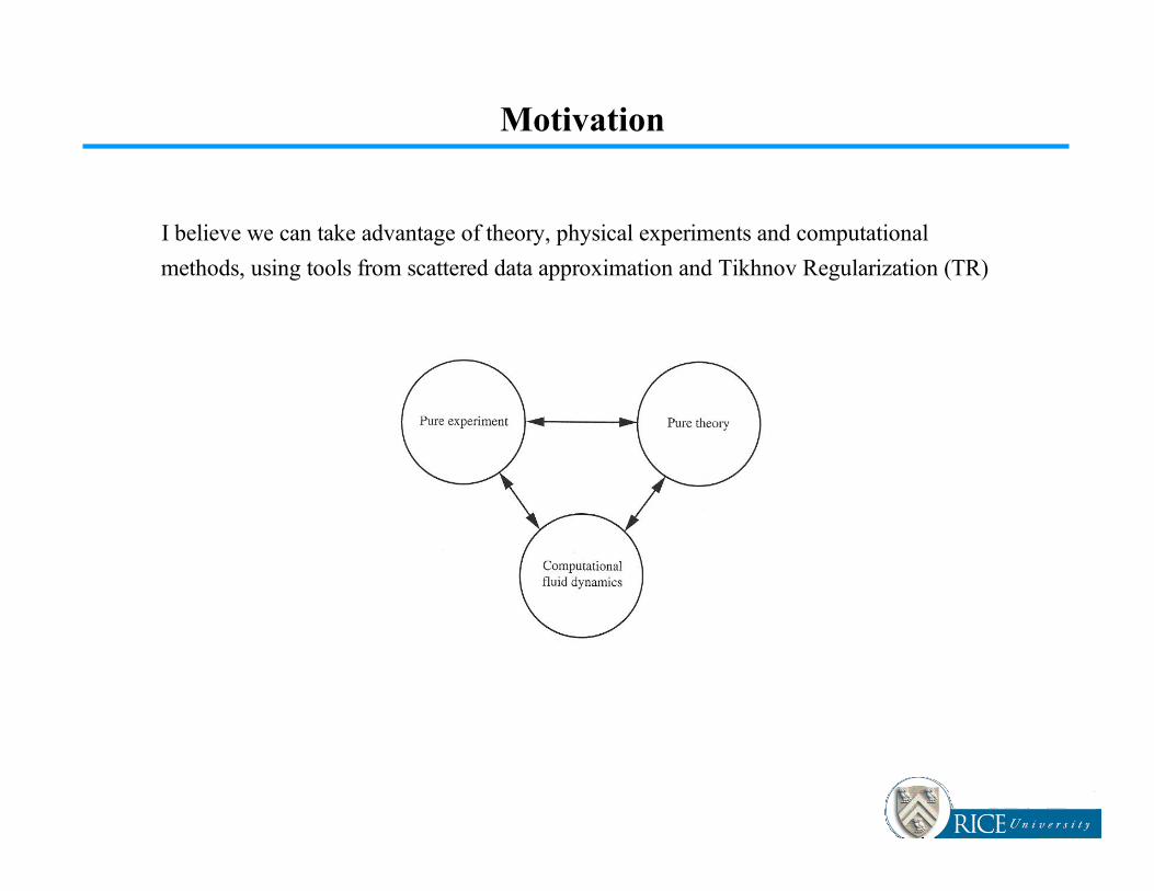
I believe we can take advantage of theory, physical experiments and computational

methods, using tools from scattered data approximation and Tikhnov Regularization (TR)

Motivation

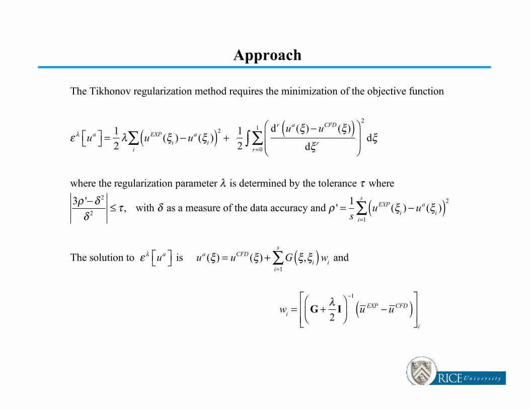
Approach

The Tikhonov regularization method requires the minimization of the objective function

ελ ua⎡⎣ ⎤⎦ =1

2λ uEXP (ξ

i)− ua (ξ

i)( )2

+i∑

1

2

dr ua (ξ)− uCFD (ξ)( )dξ r

⎛

⎝⎜⎜

⎞

⎠⎟⎟

2

dξr=0

1

∑∫

where the regularization parameter λ is determined by the tolerance τ where

3ρ '−δ 2

δ 2≤ τ , with δ as a measure of the data accuracy and ρ ' = 1

suEXP (ξ

i)− ua (ξ

i)( )2

i=1

s

∑

The solution to ελ ua⎡⎣ ⎤⎦ is ua (ξ) = uCFD (ξ)+ G ξ,ξi( )w

ii=1

s

∑ and

wi= G + λ

2I

⎛⎝⎜

⎞⎠⎟

−1

u EXP − u CFD( )⎡

⎣⎢⎢

⎤

⎦⎥⎥

i

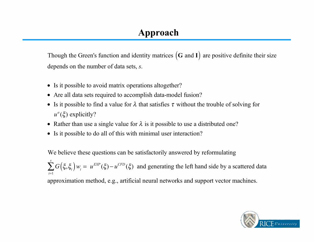
Approach

Though the Green's function and identity matrices G and I( ) are positive definite their size

depends on the number of data sets, s.

• Is it possible to avoid matrix operations altogether?

• Are all data sets required to accomplish data-model fusion?

• Is it possible to find a value for λ that satisfies τ without the trouble of solving for

ua (ξ) explicitly?

• Rather than use a single value for λ is it possible to use a distributed one?

• Is it possible to do all of this with minimal user interaction?

We believe these questions can be satisfactorily answered by reformulating

G ξ,ξi( )w

ii=1

s

∑ = uEXP (ξ)− uCFD (ξ) and generating the left hand side by a scattered data

approximation method, e.g., artificial neural networks and support vector machines.

Approach

The Sequential Function Approximation (SFA) network is our approach to

scattered data approximation.

SFA is a variation of Orr's Forward Selection training method and

Platt's Resource Allocating network that seeks to inprove the computational efficiency

through the Method of Weighted Residuals (MWR).

rn(ξ ,σ

n,c

n) = u(ξ )− u

na (ξ )= u(ξ )− u

n−1a (ξ )− w

nh(σ

n,c

n)

= rn−1

− wnh

n

The objective is to determine wn, σ

n, and c

n that minimize the residual r

n. Through the

MWR we can reformulate the residual equation as a minimization problem,

Rn, R

n= R

n−1, R

n−1− 2w

nR

n−1,h

n+ w

n2 h

n,h

n

Approach

The solution for discrete data sets is the nonlinear minimization of

1−(r

n−1⋅H

n)2

(Hn⋅H

n)(r

n−1⋅r

n−1)

where σn, and c

n are unconstrained with w

n=

(Rn−1

⋅Hn)

(Hn⋅H

n)

.

The network parameters wn, σ

n, and c

n account for one network unit at the nth iteration.

With an initial σn is set, the algorithm begins and with the determination of w

n, σ

n, and c

n

a new basis function is allocated and rn is updated.

The iterative process continues until either a pre-determined tolerance is reached

max |rn−1

| ≤ τ( ) or n = s.

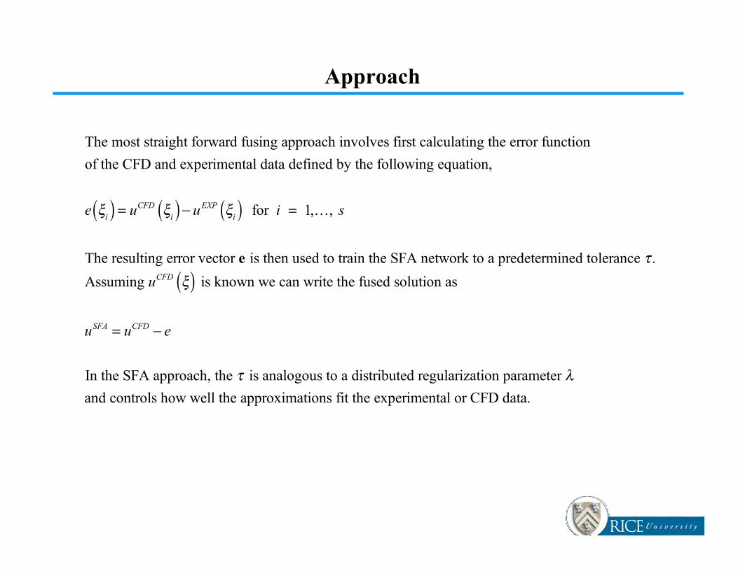
Approach

The most straight forward fusing approach involves first calculating the error function

of the CFD and experimental data defined by the following equation,

e ξi( ) = uCFD ξ

i( )− uEXP ξi( ) for i = 1,…, s

The resulting error vector e is then used to train the SFA network to a predetermined tolerance τ .

Assuming uCFD ξ( ) is known we can write the fused solution as

uSFA = uCFD − e

In the SFA approach, the τ is analogous to a distributed regularization parameter λand controls how well the approximations fit the experimental or CFD data.

Approach

This work follows from our efforts in manual and "hands-free" neural network

programming and meshfree finite element modeling.

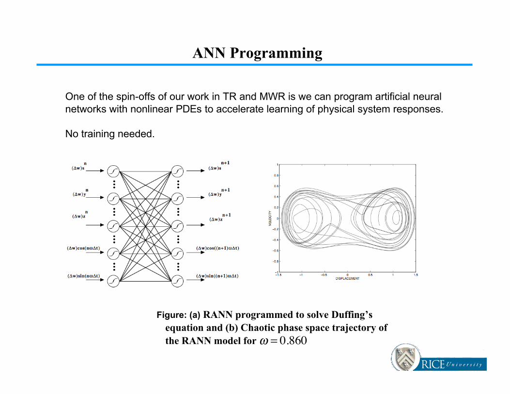
One of the spin-offs of our work in TR and MWR is we can program artificial neuralnetworks with nonlinear PDEs to accelerate learning of physical system responses.

No training needed.

Figure: (a) RANN programmed to solve Duffing’sequation and (b) Chaotic phase space trajectory ofthe RANN model for

�

ω = 0.860

ANN Programming

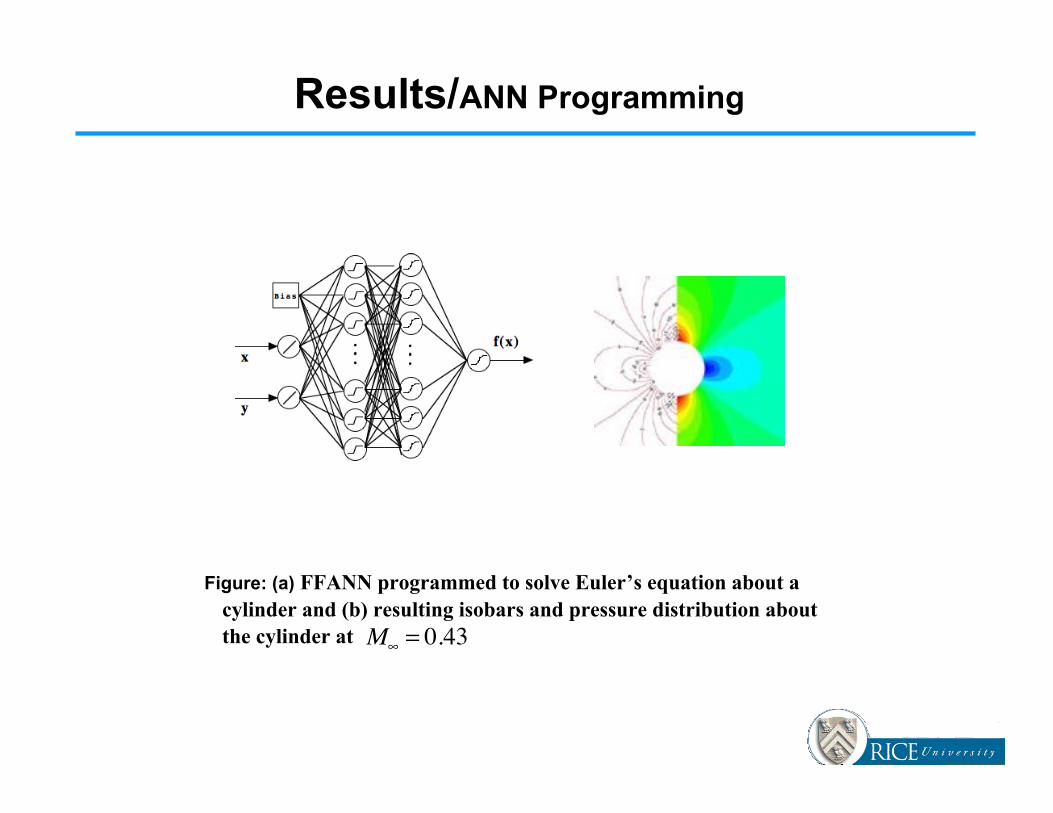
Results/ANN Programming

Figure: (a) FFANN programmed to solve Euler’s equation about acylinder and (b) resulting isobars and pressure distribution aboutthe cylinder at

�

M∞ = 0.43

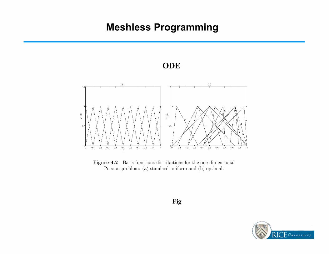
ODE

Fig

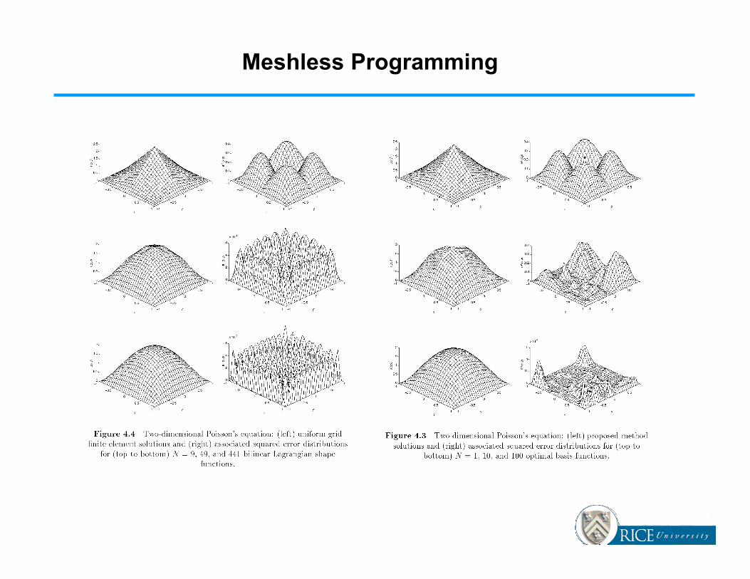
Meshless Programming

Meshless Programming

Function Approximation Test

2D exponential bases approximating an aligned and a skewed discontinuitywith (a) 1 basis and (b) 20 bases by OIA

Meshless Programming

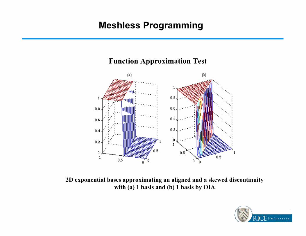
Function Approximation Test

2D exponential bases approximating an aligned and a skewed discontinuitywith (a) 1 basis and (b) 1 basis by OIA

Meshless Programming

Discrete Ordinate Method (DOM) Thermal Radiation Problem

Non-dim. temp. approx. using 21 exp.bases by meshless method

Non-dim. temp. approx. using 40401finite volume bases

Meshless Programming

Performance

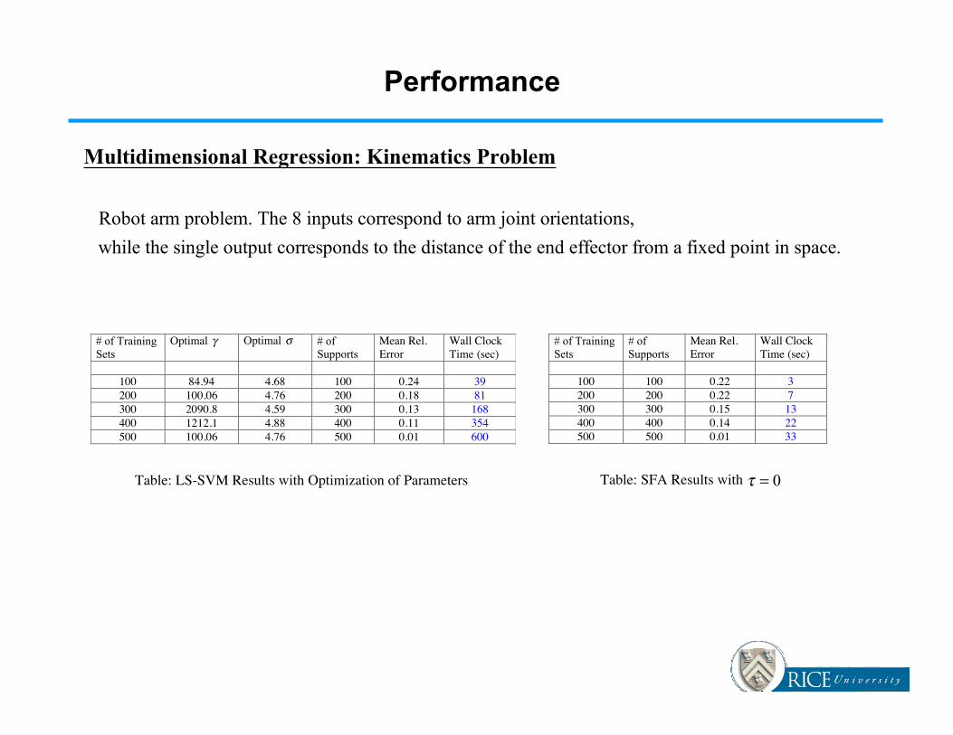
Multidimensional Regression: Kinematics Problem

Table: LS-SVM Results with Optimization of Parameters

Robot arm problem. The 8 inputs correspond to arm joint orientations,

while the single output corresponds to the distance of the end effector from a fixed point in space.

Table: SFA Results with

# of TrainingSets

Optimal γ Optimal σ # ofSupports

Mean Rel.Error

Wall ClockTime (sec)

100 84.94 4.68 100 0.24 39200 100.06 4.76 200 0.18 81300 2090.8 4.59 300 0.13 168400 1212.1 4.88 400 0.11 354500 100.06 4.76 500 0.01 600

# of TrainingSets

# ofSupports

Mean Rel.Error

Wall ClockTime (sec)

100 100 0.22 3200 200 0.22 7300 300 0.15 13400 400 0.14 22500 500 0.01 33

τ = 0

Performance

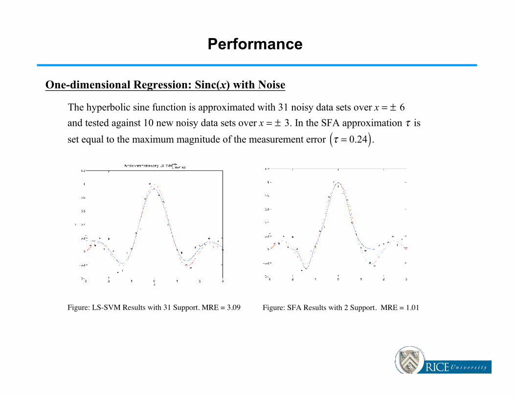
One-dimensional Regression: Sinc(x) with Noise

Figure: LS-SVM Results with 31 Support. MRE = 3.09

The hyperbolic sine function is approximated with 31 noisy data sets over x = ± 6

and tested against 10 new noisy data sets over x = ± 3. In the SFA approximation τ is

set equal to the maximum magnitude of the measurement error τ = 0.24( ).

Figure: SFA Results with 2 Support. MRE = 1.01

Performance

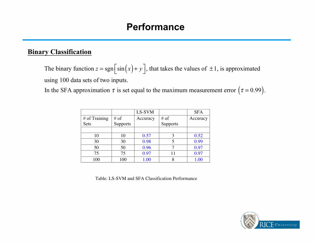
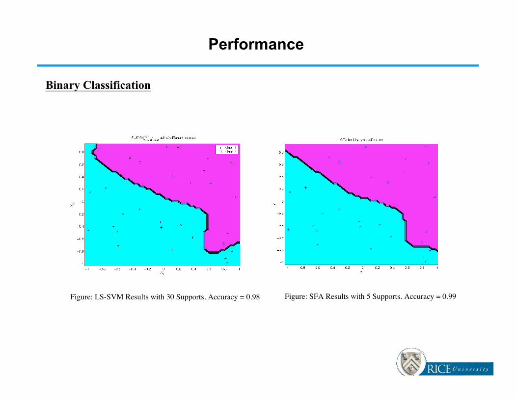
Binary Classification

Table: LS-SVM and SFA Classification Performance

The binary function z = sgn sin x( ) + y⎡⎣ ⎤⎦ , that takes the values of ±1, is approximated

using 100 data sets of two inputs.

In the SFA approximation τ is set equal to the maximum measurement error τ = 0.99( ).

LS-SVM SFA# of TrainingSets

# ofSupports

Accuracy # ofSupports

Accuracy

10 10 0.57 3 0.5230 30 0.98 5 0.9950 50 0.96 7 0.9775 75 0.97 11 0.97100 100 1.00 8 1.00

Performance

Binary Classification

Figure: LS-SVM Results with 30 Supports. Accuracy = 0.98 Figure: SFA Results with 5 Supports. Accuracy = 0.99

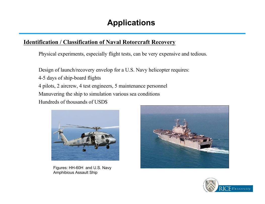
Figures: HH-60H and U.S. NavyAmphibious Assault Ship

Applications

Physical experiments, especially flight tests, can be very expensive and tedious.

Design of launch/recovery envelop for a U.S. Navy helicopter requires:

4-5 days of ship-board flights

4 pilots, 2 aircrew, 4 test engineers, 5 maintenance personnel

Manuvering the ship to simulation various sea conditions

Hundreds of thousands of USD$

Identification / Classification of Naval Rotorcraft Recovery

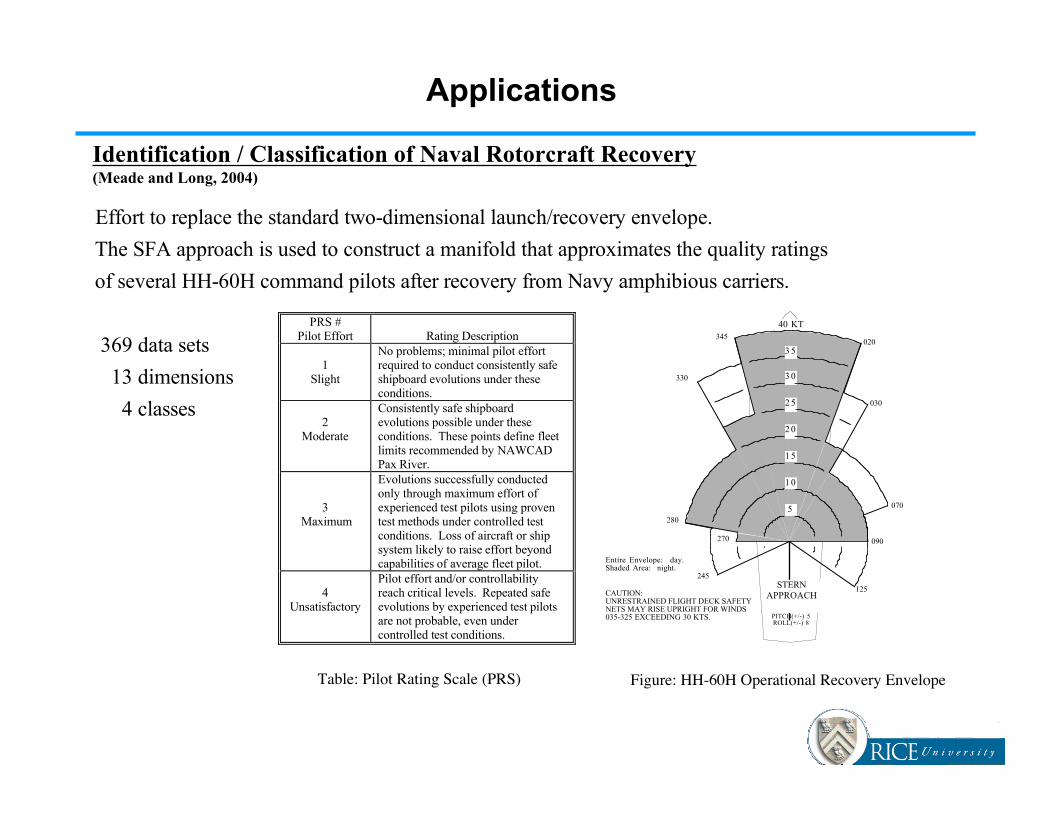
Identification / Classification of Naval Rotorcraft Recovery(Meade and Long, 2004)

Effort to replace the standard two-dimensional launch/recovery envelope.

The SFA approach is used to construct a manifold that approximates the quality ratings

of several HH-60H command pilots after recovery from Navy amphibious carriers.

369 data sets

13 dimensions

4 classes

Applications

CAUTION:UNRESTRAINED FLIGHT DECK SAFETYNETS MAY RISE UPRIGHT FOR WINDS035-325 EXCEEDING 30 KTS.

Entire Envelope: day.Shaded Area: night.

PITCH(+/-) 5ROLL(+/-) 8

5

1 0

1 5

2 0

2 5

3 0

3 5

40 KT

STERNAPPROACH

345

330

280

245

125

070

030

020

270 090

PRS #Pilot Effort Rating Description

1Slight

No problems; minimal pilot effortrequired to conduct consistently safeshipboard evolutions under theseconditions.

2Moderate

Consistently safe shipboardevolutions possible under theseconditions. These points define fleetlimits recommended by NAWCADPax River.

3 Maximum

Evolutions successfully conductedonly through maximum effort ofexperienced test pilots using proventest methods under controlled testconditions. Loss of aircraft or shipsystem likely to raise effort beyondcapabilities of average fleet pilot.

4Unsatisfactory

Pilot effort and/or controllabilityreach critical levels. Repeated safeevolutions by experienced test pilotsare not probable, even undercontrolled test conditions.

Table: Pilot Rating Scale (PRS) Figure: HH-60H Operational Recovery Envelope

Applications

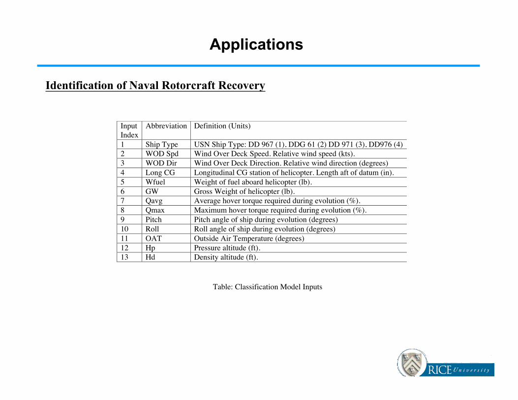
InputIndex

Abbreviation Definition (Units)

1 Ship Type USN Ship Type: DD 967 (1), DDG 61 (2) DD 971 (3), DD976 (4)2 WOD Spd Wind Over Deck Speed. Relative wind speed (kts).3 WOD Dir Wind Over Deck Direction. Relative wind direction (degrees)4 Long CG Longitudinal CG station of helicopter. Length aft of datum (in).5 Wfuel Weight of fuel aboard helicopter (lb).6 GW Gross Weight of helicopter (lb).7 Qavg Average hover torque required during evolution (%).8 Qmax Maximum hover torque required during evolution (%).9 Pitch Pitch angle of ship during evolution (degrees)10 Roll Roll angle of ship during evolution (degrees)11 OAT Outside Air Temperature (degrees)12 Hp Pressure altitude (ft).13 Hd Density altitude (ft).

Identification of Naval Rotorcraft Recovery

Table: Classification Model Inputs

Applications

Identification of Naval Rotorcraft Recovery

Figure: SFA recovery model using τ=0.16 and 201 radial bases: (a) approximation of PRS for recovery,

(b) approximation error, (c) convergence rate of the residual, (d) input sensitivity.

Most sensitive to: GW, Wfuel, and Hd.

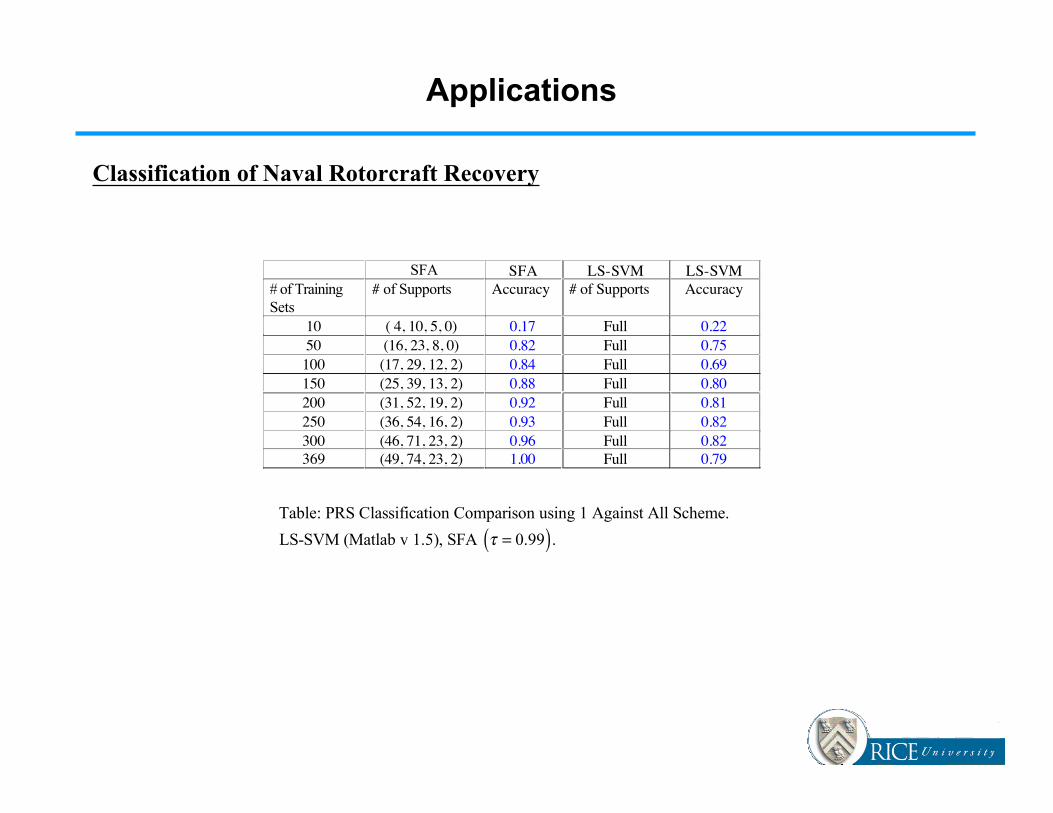
Classification of Naval Rotorcraft Recovery

Applications

SFA SFA LS-SVM LS-SVM # of Training Sets

# of Supports Accuracy # of Supports Accuracy

10 ( 4, 10, 5, 0) 0.17 Full 0.22 50 (16, 23, 8, 0) 0.82 Full 0.75 100 (17, 29, 12, 2) 0.84 Full 0.69 150 (25, 39, 13, 2) 0.88 Full 0.80 200 (31, 52, 19, 2) 0.92 Full 0.81 250 (36, 54, 16, 2) 0.93 Full 0.82 300 (46, 71, 23, 2) 0.96 Full 0.82 369 (49, 74, 23, 2) 1.00 Full 0.79

Table: PRS Classification Comparison using 1 Against All Scheme.

LS-SVM (Matlab v 1.5), SFA τ = 0.99( ).

Applications

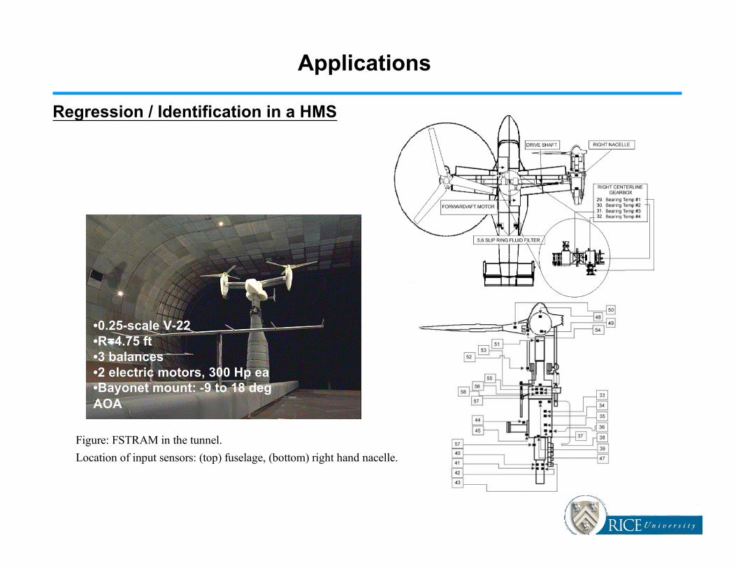
The health monitoring system we have investigated belongs to the Full-Span Tilt-rotor

Aeroacoustic Model (TRAM) used in the NASA Ames 40 × 80 ft Windtunnel.

324 data sets

71 inputs

5 targets

τ = 0.001

Regression / Identification in a Health Monitoring System(Meade, 2003)

Figure: Full Span Tilt Rotor Aeroacoustic Model configuration and schematic

Acoustic Traverses

•0.25-scale V-22•R=4.75 ft•3 balances•2 electric motors, 300 Hp ea•Bayonet mount: -9 to 18 degAOA

Applications

Figure: FSTRAM in the tunnel.

Location of input sensors: (top) fuselage, (bottom) right hand nacelle.

Regression / Identification in a HMS

Applications

Regression / Identification in a HMS

Figure: Nacelle transmission #4 bearing with 265 supports and τ = 2

(a) time series model of the temperature, (b) approximation error, (c) convergence rate, and

(d) input sensitivity.

Most sensitive to motor RPM.

Applications

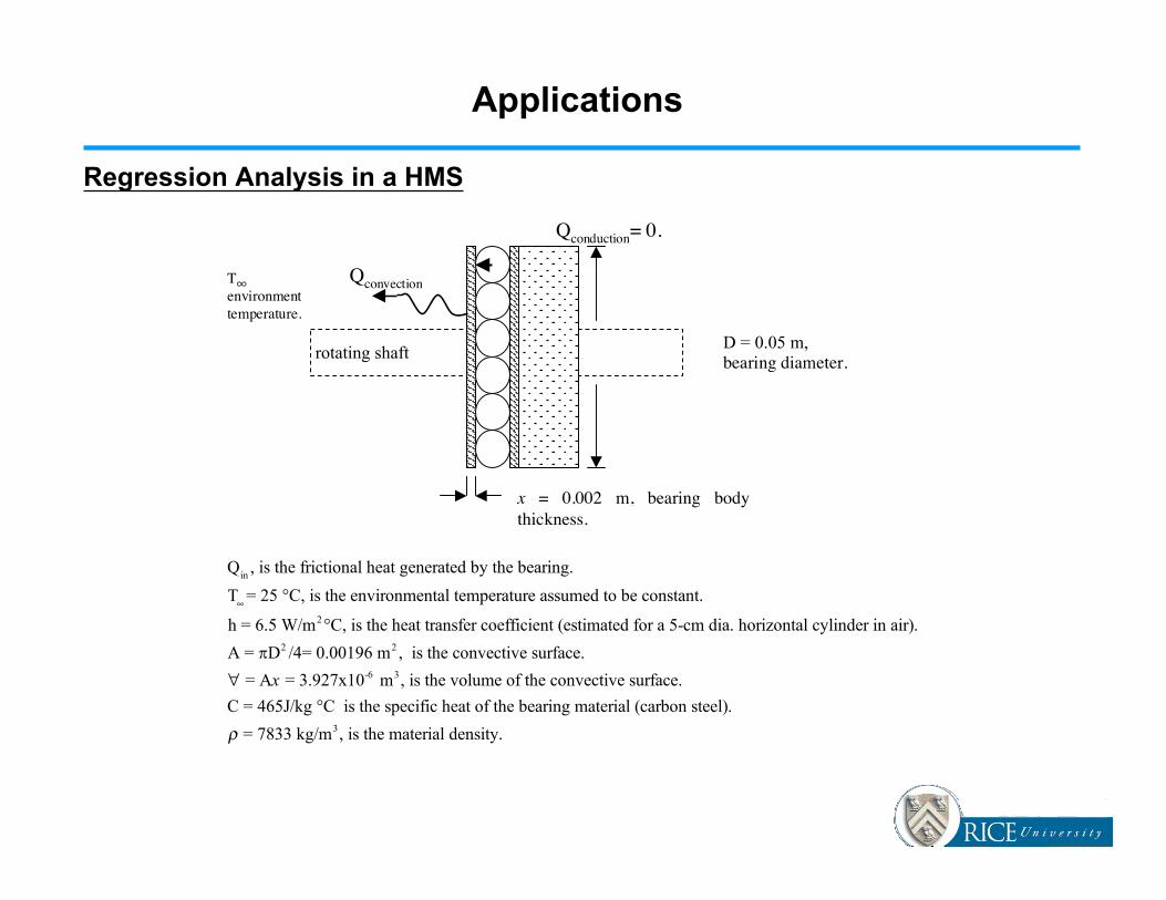
Regression Analysis in a HMS

Qconvection

Qconduction= 0.

D = 0.05 m,bearing diameter.

T∞environmenttemperature.

rotating shaft

x = 0.002 m, bearing bodythickness.

Qin

, is the frictional heat generated by the bearing.

T∞ = 25 °C, is the environmental temperature assumed to be constant.

h = 6.5 W/m2 °C, is the heat transfer coefficient (estimated for a 5-cm dia. horizontal cylinder in air).

A = !D2 /4= 0.00196 m2 , is the convective surface.

∀ = Ax = 3.927x10-6 m3, is the volume of the convective surface.

C = 465J/kg °C is the specific heat of the bearing material (carbon steel).

ρ = 7833 kg/m3, is the material density.

Applications

Regression Analysis in a HMS

Ti= T∞ +

Qin− Q

in− hA(T

i−1−T∞ )( )

hAexp −

hA(ti− t

i−1)

cρ∀⎡

⎣⎢

⎤

⎦⎥

The heat generated by the bearing, Qin

, is determined by the friction equation,

Qin= (µ ⋅ L ⋅r) ⋅ GR ⋅Ω

i⋅ 2π

60

⎛⎝⎜

⎞⎠⎟

, Watts

where

µ = 0.002 : is the friction coefficient estimate (obtained from bearing manufacturer)

L : is the frictional load in Newtons (dependent on the bearing location)

r = 0.025 m : is the bearing radius

GR : is the transmission gear reduction constant and depends on the bearing location.

Ωi : is the operating RPM.

L is determined from our sensitivity analysis of the SFA model.

Applications

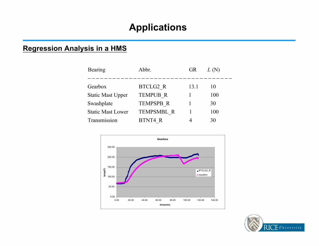
Regression Analysis in a HMS

Bearing Abbr. GR L (N)

− − − − − − − − − − − − − − − − − − − − − − − − − − − − − − − − − − −Gearbox BTCLG2_R 13.1 10

Static Mast Upper TEMPUB_R 1 100

Swashplate TEMPSPB_R 1 30

Static Mast Lower TEMPSMBL_R 1 100

Transmission BTNT4_R 4 30

Gearbox

0.00

50.00

100.00

150.00

200.00

250.00

0.00 20.00 40.00 60.00 80.00 100.00 120.00 140.00

time(min)

temp(F)

BTCLG2_R

equation

Applications

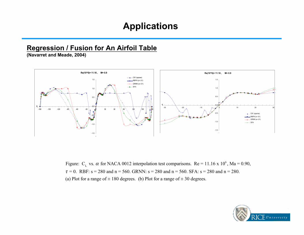
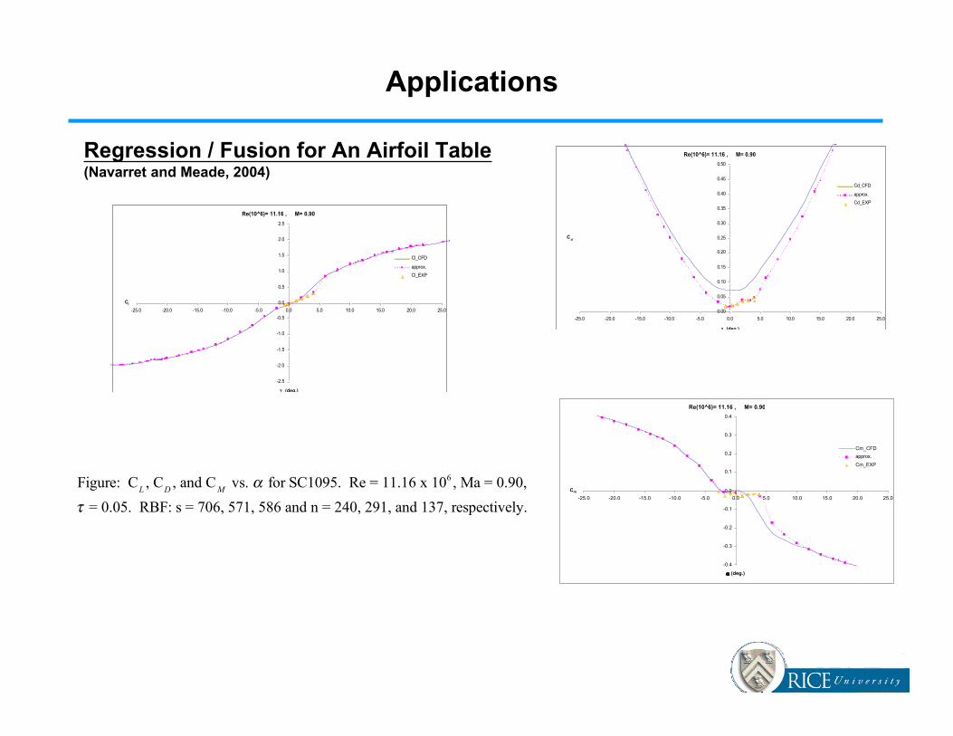
Regression / Fusion for An Airfoil Table(Navarret and Meade, 2004)

Figure: CL

vs. α for NACA 0012 interpolation test comparisons. Re = 11.16 x 106 , Ma = 0.90,

τ = 0. RBF: s = 280 and n = 560. GRNN: s = 280 and n = 560. SFA: s = 280 and n = 280.

(a) Plot for a range of ± 180 degrees. (b) Plot for a range of ± 30 degrees.

Re(10^6)= 11.16 , M= 0.9

-1.5

-1.0

-0.5

0.0

0.5

1.0

1.5

-180 -150 -120 -90 -60 -30 0 30 60 90 120 150 180

?

Cl

C81 (sparse)

RBFN (s=.01)

GRNN (s=.01)

SFA

Re(10^6)= 11.16 , M= 0.9

-1.5

-1.0

-0.5

0.0

0.5

1.0

1.5

-30 -20 -10 0 10 20 30

?

Cl

C81 (sparse)

RBFN (s=.01)

GRNN (s=.01)

SFA

Applications

Regression / Fusion for An Airfoil Table(Navarret and Meade, 2004)

Figure: CL, C

D, and C

M vs. α for SC1095. Re = 11.16 x 106 , Ma = 0.90,

τ = 0.05. RBF: s = 706, 571, 586 and n = 240, 291, and 137, respectively.

Re(10^6)= 11.16 , M= 0.90

-2.5

-2.0

-1.5

-1.0

-0.5

0.0

0.5

1.0

1.5

2.0

2.5

-25.0 -20.0 -15.0 -10.0 -5.0 0.0 5.0 10.0 15.0 20.0 25.0

? (deg.)

Cl

Cl_CFD

approx.

Cl_EXP

Re(10^6)= 11.16 , M= 0.90

0.00

0.05

0.10

0.15

0.20

0.25

0.30

0.35

0.40

0.45

0.50

-25.0 -20.0 -15.0 -10.0 -5.0 0.0 5.0 10.0 15.0 20.0 25.0

? (deg.)

Cd

Cd_CFD

approx.

Cd_EXP

Re(10^6)= 11.16 , M= 0.90

-0.4

-0.3

-0.2

-0.1

0.0

0.1

0.2

0.3

0.4

-25.0 -20.0 -15.0 -10.0 -5.0 0.0 5.0 10.0 15.0 20.0 25.0

α (deg.)

Cm

Cm_CFD

approx.

Cm_EXP

Conclusions & Future Work

The TR with MWR framework shows some promise as a way to merge theory,

experimental observations, and computational fluid dynamics.

We have shown it is possible to form ua (ξ) with little user interaction.

Further investigation of the method and the applications are required:

• Perform meshless solution of ua (ξ) with uCFD (ξ) and uEXP (ξi) together.

This would produce meshless and data-driven computational mechanics solver.

• Investigate method in designing better experiments.

• Investigate the method with proxy data.

• Investigate other types of bases.