an accuracy adjustment of gis data by using a data fusion ... · school relationship between kut...

An Accuracy Adjustment of GIS Data by Using A Data

Fusion Method

January 2002

Supervisor Associate Professor Masataka TAKAGI

Department of Infrastructure System Engineering Kochi University of Technology

Kochi, Japan 1045032

Jong Hyeok JEONG

ABSTRACT

Nowadays, many companies and local governments have produced various GIS data. But most of them were shared or sold without a specification or a metadata. When those data overlaid with officially used high accuracy data, some errors appeared. Therefore, usually an uncertain GIS data, which does not have accuracy information, cannot be used with a high accuracy directly. In this study, the accuracy of the bridge database was adjusted by the intersections of rivers and roads data in officially used GIS data. Then distances between bridges and intersections of roads and rivers were calculated. If bridge length with positional accuracy is shorter than the distance between the bridge point and the nearest intersection, it was assumed that the bridge point does not have enough accuracy to be adjusted. By the GIS data fusion method, the accuracy of 60% of bridges over river was adjusted and obtained clear accuracy. The result of accuracy adjustment of the bridge database classified according to its road attribute, then the result of accuracy adjustment of the bridge database was assessed by the classification result. The result of accuracy adjustment by data fusion method was successfully assessed by the attribute data of the bridge database.

ACKNOWLEDGE

First of all, I would like to appreciate god because I have my family who love me. Without

their great love, I could not finish this master course. And I would like to appreciate associate

professor Takagi MASATAKA who is my supervisor, he gave me much inspiration in my research

and planted positive thinking in my mind. Because of his support and teaching, I could take part in

the JSPRS and ACRS. Thank you very much sir!

When I just came here, I had to study the java programming language for my research. But

there was no one who could teach me the programming language in English. Fortunately, I could

contact a professor in the Depart. His name is P. H. P. Bhatt. He taught me the programming

language like a private tutor. It was great experience for me. His teachings are alive in the appendix

II and III, god bless you! pf. Bhatt. When I just came here, Korean students in Kochi University took

care of Kim and me, I can’t forget their help, until I die, thanks Dr. Hyang Sook CHOI, Dr. Hee soon

CHOI and doctor candidate Mu Gwun LEE. I hope their great success in Korea. I have friends from

Thailand; Supakit SWATEKITITHAM, Jirapong PIPATTANADIWONG, Thammannon

DENPONGPAN, thanks for your kindness and teaching.

Professor Hyung Lae LEE, Eun Kyong SUGIYAMA, they promoted the sister

school relationship between KUT and National University of Chinju, I would like to

appreciate Pf. Myung An Park, Nam Hyung RYU, Ho Chul Kang, Choon Suk LEE and

Tae Kyoon KIM.

Fortunately, I became a student of the rotary club scholarship program. The

rotary club foundation provided not only scholarship but also assigned a volunteer to me.

The volunteers are Shin UETA and Mitchi UETA. They taught me many things about

Japan; Japanese Culture, Japanese language and so on. I cannot forget their kindness.

LIST OF CONTENTS

1. Introduction 1.1 Background 1 1.2 Statement of Problem 1 1.3 Previous Study 3 1.4 Objectives 4 1.5 Scope of Study 4

2. Used data sets and computer programs 2.1 General 5 2.2 National Land Digital Information 5 2.3 Bridge Database 6

2.4 Disaster Prevention Information 8 2.5 Used Programs 8

3. Methodology 3.1 General 9 3.2 Preprocessing 9 3.3 Accuracy Adjustment Outline 10 3.4 Generation of Intersections 11 3.5 Finding Nearest Intersection 12 3.6 Overlay 14 3.7 Distance Calculation 17 3.8 Specifying Error Information in The Database 17 3.9 Accuracy Adjustment by Fusion Method 18 3.10 Accuracy Assessment 19

4. Results 4.1 The Result of Preprocessing 21 4.2 Generating Intersection 21 4.3 The Identification of Error Sources on the overlay 21 4.4 Distance Calculation 22 4.5 Matching and Registering 25 4.6 Specifying Error Information in Database 26 4.7 Accuracy Adjustment by Data Fusion Method 27

4.8 Accuracy Assessment 28

5. Conclusions and discussion Conclusion1 31 Conclusion2 32 Conclusion3 33 Conclusion4 34 Conclusion5 34 Further Study 35

Reference Appendix I : Literature Review 39 Appendix II : Program for Overlapped Bridges Detection 52 Appendix III : The Program for One to One Relationship 57

LIST OF FIGURES

3-1. Preprocessing procedures 10 3-2. The outline for accuracy adjustment 11 3-3. Before generating intersections 12 3-4. After generating intersections 12 3-5. The nearest feature calculation 13 3-6. Bridge points on DPI 15 3-7. Bridge points on NLDI distance mapping 16 3-8.The criterion of accuracy adjustment 19 3-9. Data fusion 20 3-10. The three categories in the road attribute of the bridge database 20 4-1. Errors from coordinate mistyping 22 4-2. The histogram of frequency of bridge in distance calculation 23 4-3. Boxplots of distance calculation result 24 4-4. Boxplots of the distance calculation result (less than 530m) 24 4-5. Plotted bridge length and the distance from each bridge

to the nearest intersection 25 4-6. Accuracy adjustment results in slope 29 4-7. Classified bridges on slope analysis result of Kochi prefecture area 30 5-1. Slivers: the classic form of overlay error 32 5-2. Modified hierarchy of need for modeling errors in GIS 33 A-1. The life cycle of a soil database 40 A-2. A hierarchy of needs for modeling error in GIS operations 40 A-3. Slivers: the classic form of overlay error 41 A-4. Another case of overlay error 42 A-5. A simplified visualization of statistical precision, accuracy, and bias 47

LIST OF TABLES

2-1. Included information in land digital information 6 2-2. Summary of metadata 6 2-3. The number of bridge which does not have its length information 7 2-4. The number of bridges on river, not on river and others 7 2-5. The number of overlapped bridges 7 3-1. Distance calculation result table 14 4-1. The example of arrangement result of making one-to-one relationship 26 4-2. Specified error and the result of matching (sample) 27 4-3. Accuracy adjustment result by fusion method (sample) 28 4-4. The result of accuracy adjustment 28 A-1.The separation error into time phases and sources 45 A-2 Relationship Between Scale, Accuracy and Resolution 45

1 INTRODUCTION CHAPTER 1

CHAPTER 1 INTRODUCTION

1.1 Background

GIS users suffered from transferring a GIS format to another data format.

Therefore, new movement appeared to make a vendor-neutral GIS data format by using XML protocol. Open GIS organization in America established GML, and the Ministry of Economy and Industry in Japan established G-XML which was adapted as a standard GIS data format. It enables GIS users to overlay and integrate various GIS data from local governments, companies and organizations. Although standard GIS data format environment was established, there appeared a problem of accuracy.

The Department of Construction in Kochi prefecture established a bridge

database and shared the data without accuracy information. When the bridge database was overlaid with another GIS data based on different scales, positional errors appeared. Usually bridges on river exist on the intersection of road and river. However when the data was overlaid with official high accuracy GIS data, bridge points did not match with the intersection of road and river or lay with the circle of positional error tolerance. Therefore, the data needed some accuracy adjustment to be used with high accuracy GIS data.

1.2 Statement of Problem

Two GIS capabilities, which excite enthusiasm among potential user are the

ability to change map scale and the ability to overlay map at random. Both capabilities are indeed exceedingly useful; they constitute muｃh of the comparative advantage GIS holds over spatial analysis based on analogue maps. Both capabilities may also mislead decision makers who are unaware of the imprecision inherent in all cartography and who are untutored in the ways errors compound when map scales are changed or when

maps are merged (Abler, 1987 p.305) )1 .

The main motivation for interest in the accuracy of spatial databases comes from an applied perspective – the problem is real, and we need better methods for addressing it. Besides basic research, we need greater sensitivity to error on the part of GIS users, greater awareness of the kinds of errors, which can occur, and techniques for


recognizing and perhaps reducing their impact. Finally, the problem is also technical, in the sense that we need explicit methods of tracking and reporting error in GIS software, and algorithms and data structures which recognize uncertainty and inaccuracy directly. In short we need greater sensitivity to accuracy issues among GIS designers and developers (Accuracy of Spatial Databases, edited by Michael Goodchild and Sucharita

Gopal, p1, 1989) )2 .

The widespread availability of Geographic Information System has enabled many users to integrate geographic information from a wide range of sources. An inevitable of equal quality that it can contain errors and uncertainty those need to be recognized and properly dealt with (Giulio Maffini, Michael Arno and Wolfgang

Bitterlich , 1989) )3 .

In reality a GIS may encourage poor analysis by separating the data collection, compilation and analysis functions, and failing to make the user aware of the possible danger of indiscriminate use of such functions as scale change, reclassification and

overlay (Michael F. Goodchild, 1989). )4

It seems likely that all spatial data and all types of spatial analysis contain some type of error. Therefore it is impossible to perform error- free spatial analysis and it becomes the task of spatial analysts to reduce error to the point at which it does not interfere which the conclusions drawn from a particular analysis (A. Stewart

Fotheringham, 1989) )5 .

It is important to recognize the type, severity and implications of errors that are

inherent in the use of a geographic information system (Giulio Maffini, 1989) )6 .

The effects of combining data characterized by differing levels of error and

uncertainty need to be identifiable in the final outputs (Stan Openshaw, 1989) )7 .

GIS has taken an important role in various fields, and it already has become

familiar to end-users, but they use it without knowing or recognizing its detail accuracy or errors. Because of this reason, many researchers have warned GIS developers and users about the errors in GIS and emphasized the necessity of reporting, quantifying or tracking errors.


1.3 Previous Study

The literatures were reviewed that relate to errors in spatial database, accuracy assessment and adjustment, and also data fusion.

Michael F Goodchild )10 explained how errors should be treated in GIS data updating. Howard Vergin )11 introduced a hierarchy of needs for modeling error in GIS operation. Some errors from overlaying digital maps were investigated by Nicholas R.

and Chrisman )13 . What types of errors exist in GIS data and types of errors that can appear have been investigated. Recognizing and specifying errors in GIS that prevent users from being misled by error prone GIS were considered. Errors in experimental data need to be investigated in the hierarchy of need for modeling errors for GIS operation. From the investigation, some accuracy adjustment direction and criteria will be established (Appendix I).

On going problems for spatial uncertainty researches are following. 1) uncertainty representation for discrete models of issues in spatial

uncertainty for continuous models of spatial variability. 2) the need to make accuracy assessments more accessible to users of spatial

data and model predictions. 3) the effect of scale on uncertainty. 4) how uncertainty estimates from different disciplines can be combined to

provide a composite estimate of uncertainty in final products. Frequently the need arises to analyze missed spatial databases, and mixed data

sets consist of satellite spectral, topographic and other points from data. All registered geometrically mixed data, as might be found in a geographic information system. So far, many remotely sensed data were used to merge with other sources for a special purpose.

For example, Srinivasan and Ricahrd (1993) )8 able to analyze the images jointly and thus develop a cover type map that resolves classes that are confused in either the Landsat or radar data alone. A simple methodology has been developed for raster-to-vector for use in a GIS. This methodology was employed successfully to integrate both coarse and fine resolution raster image (e.g. LANDSAT MSS and TM; and SPOT HRV) into a vector GIS ( N. M. Mattikalli. B. J. Devereux and K. S. Richards,

1995) )9 . But it is very rare that a GIS data merged with another data. There is


possibility to merge between the coordinates of high accuracy data and the attribute data of a low accuracy data. There will be advantages in using a data fusion method, if we introduce data fusion in GIS. In order to find the potential and possibility of using a fusion method in GIS, the data fusion method focused on especially the accuracy adjustment of a GIS data in this study (Appendix I).

1.4 Objectives

Usually, bridge, dam and so on have low accuracy in spatial data because of their spatial characteristic because it has long error radii. So the accuracy of those kinds of objects can be adjusted by computer works instead of surveying. In the remote sensing field, many researchers have studied about the data fusion of various satellite images that were generated by different sensors. However, much works has been reported on the usage of the data fusion method in GIS. Thus, objectives in this study are:

1) To adjust the accuracy of a GIS data which does not have accuracy information by using a data fusion method.

2) To improve the reusability of an uncertain GIS data.

3) To find optimized procedure of the accuracy adjustment methods in

the data fusion method.

4) To assess the accuracy adjustment result with attribute data.

1.5 Scope of The Study In the whole process of accuracy adjustment of a GIS data, method of adjusting

the accuracy of a GIS data on computer work removing the uncertainty of a GIS data were investigated.

5 USED DATA SETS AND COMPUTER PROGRAMS CHAPTER 2

CHAPTER 2 USED DATA SETS AND COMPUTER PROGRAMS

2.1 General

Before making accuracy adjustment in the bridge database, the understandings of data structure, file format, code type and such like are needed. In the Land Digital Information case, metadata was referred for the understanding of the detail information of it.

2.2 National Land Digital Information (NLDI)

In accuracy adjustment, the National Land Digital Information (NLDI) was used as a reference data because it had clear accuracy information and metadata. The NLDI was required to investigate the contents and data structure of it.

The NLDI was established by the Ministry of Land, Infrastructure and Transport in the year of 1930. Currently it is still being updated. The data is being used as an infrastructure information in various fields (for example, government land use planning, government land planning, urban planning and so on). It includes various kinds of information (Table 2-1). Some parts of the data were established by another organization, for example Japan Coast Guard, Geographical Surveying Institute.

At present, the data is being shared by the Ministry of Land, Infrastructure and Transport to support researchers, decision makers, and government organizations, local governments and universities with free of charge. Kochi Software Center (a government organization) handed us the data that covers Kochi prefecture area. Two themes were included in the data, one was the road data, and the other is the river, and both based on 1:25,000 scale map. The feature type of roads and rivers in NLDI was line, and its coordinate system was Cartesian coordinate system. The positional accuracy of this data was 12.5m because this data was based on a 1 to 25000 scale map (Appendix I, Table A-2).


Table 2-1 Information included in land digital information

Category Contents

Selected Area Forest, Natural Park, Reserved Area, Agricultural Industry Area

Coastal Area Harbor, Reserved Area for Water Quality, Coastal Line

Nature Climate Information Land Land Use Information

Infrastructure Road, Rail

Equipment Power Generate Station Statistic of Agriculture Statistic of Agricultural Industry

Hydrology Dam, River, Lake

The both data cover west boundary 122.93 ° , east boundary 145.82 ° , north boundary 45.52 ° and south boundary 24.04 ° . The attribute data of road are highway, national road, local government roads and national roads.

The National Land Digital Information is being distributed with a metadata (http://nlftp.mlit.go.jp/ksj/). The metadata of roads and rivers in the NLDI has following information (Table. 2-2).

Table 2-2 Summary of metadata

Metadata Category Contents

Catalog information Metadata Identifier, Title, Volume, Producer Information

Range of data set 122.93 ° (N), 145.82 ° (E), 45.52 ° (S), 24.03 ° (W) Character Code JIS Information category Hydrology, Infrastructure

Based map scale 1:25000

2.3 Bridge Database The Department of Construction in Kochi prefecture established a bridge

database for the purpose of management of bridges, and the bridge database was shared without metadata and specification. Because it was shared without metadata or


specification, the bridge database was considered as an uncertain GIS data. Its coordinate system is Geodetic coordinate system.

Bridges in the bridge database are divided into the bridges that do not have length information and others (Table. 2-3). Table 2-3 The number of bridge which does not have its length information

Numbers (points)

Bridges which do not have its length information 612

Others 735

Total 1347

The contents of the database were examined before making accuracy adjustment (Table 2-4). Table 2-4 The number of bridges over river, not over river and others

Contained Information Numbers (points)

The Bridges over Rivers 685

Bridges Not over Rivers 50 Bridges with length information 735

This bridge database cannot be used in the accuracy adjustment without

arrangement. In this study, only one bridge point should be on a corresponding position, so some overlapped points should be eliminated before accuracy adjustment (Table 2-5). In addition, bridges located only on rivers were used because their positions were adjusted by the intersections of road and river in reference data. So the bridges positioned at rivers were extracted from the bridges which have their length information. Table 2-5 The number of overlapped bridges

Numbers (points)

Overlapped Bridge 102

Not Overlapped Bridges over River 583

The Bridges located over River (total) 685


2.4 Disaster Prevention Information (DPI)

The Disaster Prevention Information (DPI) was established by the Department

of Disaster Prevention in Kochi prefecture, which was based on a 1 to 2500 scale map. In this data set, the features of roads and rivers were described by polygons. The intersections of roads and rivers in this data were used to identify the errors in the bridge database. 2.5 Used Programs

For accuracy adjustment, a commercial software and coded programs were used. The main platform program is ArcView, the bridge data base was invoked and displayed as points in this program. The data format of bridge database is “dbf” database format, and it was converted to the shape data file format, which is the data format often used in GIS.

ArcView has a native programming language, “Avenue”. It is commonly used

by GIS application producers and researchers. Environmental Systems Research Systems Research Institute (ESRI) establish an environment on web for exchanging Avenue programs, which was produced by GIS programmers and researchers (http://gis.esri.com/scripts/scripts.cfm). And ArcView users can download a program, which was optimized and customized for a particular purpose.

In this study, three Avenue programs were used; one is the “Compile Table Tools” (coded by Charles Herbold), another is the “Xtools” (coded by Mike DeLaune), and the third is the “ Nearest Feature” (coded by Jeff Jenness). These three program were obtained from ESRI (http://gis.esri.com/scripts/scripts.cfm). Compiled Table Tools enable us to manipulate table of GIS database; we can join, add, import and export tables with Compiled Table Tools. Xtools has many functions, and mainly the function of intersect-two-themes was used to make intersections. The Nearest Feature program detects the nearest object from an object, and it calculated distance between two objects and records the result in a table. Arc/Info program was used for changing coordinate systems from geodetic coordinate system to Cartesian coordinate system.

9 METHODOLOGY CHAPTER 3

CHAPTER 3 Methodology

3.1 General The hierarchy of needs for modeling error in the GIS operation concept (Figure

A-2 in Appendix I) was used to make a direction for error recognition and accuracy adjustment. On which the point of a bridge was surveyed that was not specified in the bridge database, so the center of each bridge was assumed as the actual surveyed point of each bridge. A data fusion method was used for making accuracy adjustment of the bridge database. Also their accuracy was assessed by their road attribute.

3.2 Preprocessing

As mentioned in the Chapter2, the bridge database could not be used directly

for accuracy adjustment. The file format of the bridge database cannot be used with another format of a GIS data. Therefore, preprocessing before the accuracy adjustment was necessary.

Total 685 bridges are located on rivers. Some overlapped points of them were

detected by a written program (Appendix II) and eliminated because only one point should be on a coordinate (position) in this case.

Some parts of a bridge were described as points, and they were overlapped on a

position for its structural management, so it means many points were overlapped on the same position (coordinate). In this study, only bridges over rivers were needed, because the accuracy of bridge points were adjusted by the intersection of a road and a river in a reference data.

The bridge points not over rivers were not considered in this study. The

coordinate system of the bridge database causes a problem in overlay. Because the coordinate system is the Geodetic coordinate system, it changed into the Cartesian coordinate system in order to overlay with other data sets. Finally, the database is converted to “Shape” data file format that is a common data format in GIS (Figure 3-1).


Figure 3-1 Preprocessing procedures

.

3.3 Accuracy Adjustment Outline

To identify the source of error, the intersection points of roads and rivers in the National Land Digital Information (NLDI) and the Disaster Prevention Information (DPI) were generated. The bridge points were overlaid with the intersections in the NLDI and DPI, then positional errors were observed. The nearest intersection to each bridge point was matched, and their relationship was registered the relationship of them in the bridge database. The distance from the nearest intersection in reference data to each bridge point was calculated, and the error was measured. The measurement of positional error was specified in the bridge database for error management. In the last process, the strategy for error reduction was established.


Figure 3-2 The outline for accuracy adjustment

3.4 Generation of Intersections

To identify the source of error, the bridge points in the bridge database were required to overlay with the intersections of roads and rivers in the National Land Digital Information and in the Disaster Prevention Information. ODF XTools program and Spatial Analysis (ESRI) were used to make intersection points. Figure 3-3 shows the roads and rivers in the NLDI. Figure 3-4 shows the result of intersecting roads and river in the NLDI.


Figure 3-3 Before generating intersections

Figure 3-4 After generating intersections

3.5 Finding the Nearest Intersection

The distance from each bridge point to the nearest intersection point was calculated. They were linked and registered in the bridge database and assumed the actual position of each bridge point. The Nearest Feature program (coded by Jeff Jenness) was used. It enables us to calculate the nearest feature from each object and to specify the most nearest, the next nearest and for the third nearest features.


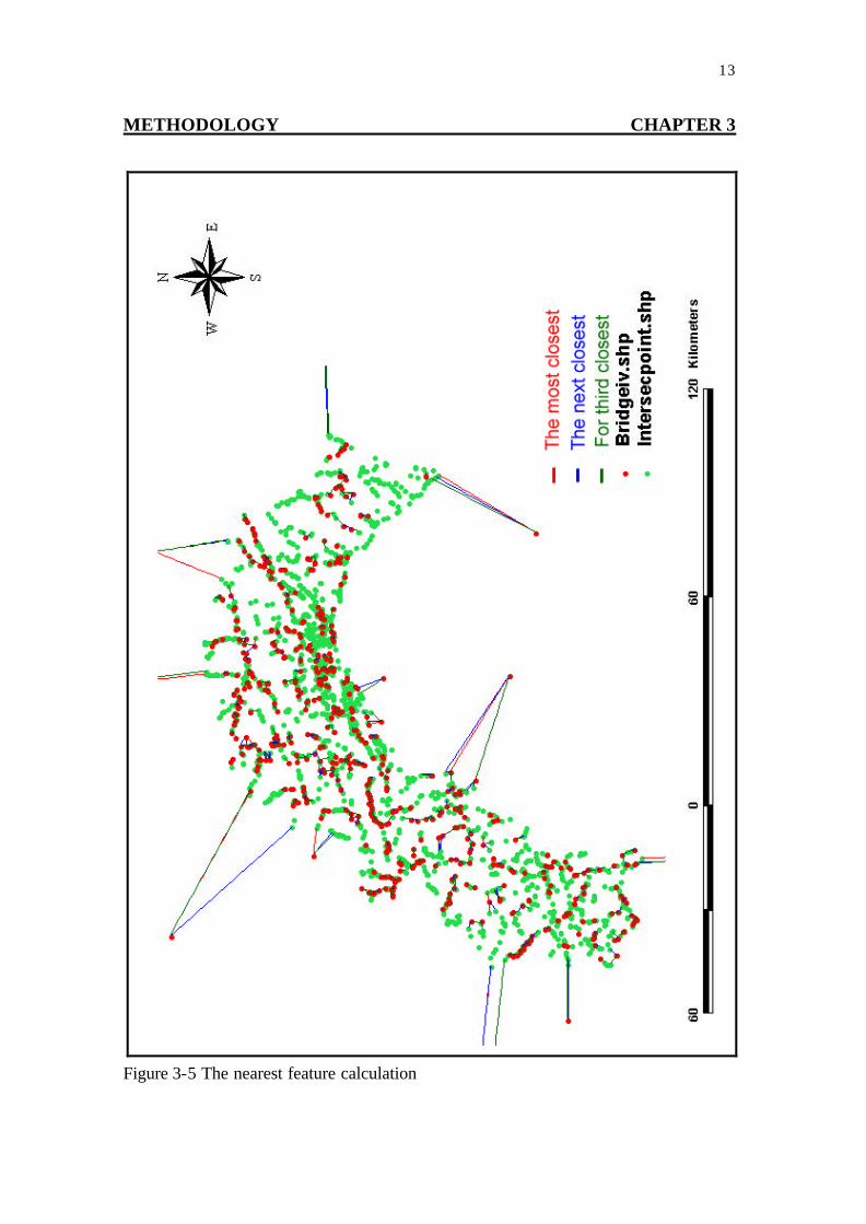
Figure 3-5 The nearest feature calculation


Figure 3-5shows the result of distance calculation. The nearest feature program detected the closest intersection, the next closest intersection, the less closest intersection from each bridge.

Table 3-1 Distance calculation result table UID is bridge’s unique ID number, 1_ID is the most nearest intersection’s ID

number and the distance between the bridge and the nearest intersection, 2_ID

is the secondly closest intersections’ ID number from a bridge point.

Table 3-1 shows an example of the result of distance calculation, Uid is the

unique identification number of each bridge, 1_ID means the nearest intersection point of identification number, the 1_C_Dist is the distance between the most nearest intersection and a bridge point, and 2_ID is the secondly closest intersections’ id. In the distance calculation result, some bridge points matched more than one intersection points, so their relationship were rearranged to make one-to-one relationship, and a program was used for the arrangement of one-to-one relationship (appendix III). 3.6 Overlay

For thematic error source identification, bridge points were overlaid with

intersection of road and river in two reference data, one is the DPI and the other is the NLDI. The feature type of the DPI is the polygon, and the generated intersection shape is almost same as bridge, so when bridge are ove rlaid with the polygon, the positional


errors were clearly shown (Figure 3-6). On the other hand, generated intersection points of roads and rivers in NLDI were overlaid with distance circle to show the existing phase of the intersect points from each bridge point (Figure 3-7). From the two overlays, the thematic errors of the bridge were recognized at a glance.

Figure 3-6 Bridge points on the DPI


Figure 3-7 Bridge points on the NLDI distance mapping


3.7 Distance Calculation

Positional Accuracy Handbook (www.mnplan.state.mn.us/press/) described

how to measure the positional error in GIS data. In the specification, positional error in GIS data was calculated by differencing x and y coordinates of reference data and x and y coordinates of points in a test data, then the error radii were calculated. In this study, the error radii were calculated directly by using the Nearest Feature Avenue Script program. In the process of finding the nearest intersection of each bridge point, the Nearest Feature program was used to calculate the distances from the nearest intersection to each bridge point. The calculated distances were used as error radii in the accuracy adjustment. Errors in this data quantified by the calculated distances.

Some bridges achieved one-to-one relationship, but they had still uncertainty in accuracy domain because some of them have the result of distance calculation, which is longer than the longest bridge in the bridge database. To select bridges, which have shorter distance than the length of the longest bridge, a threshold value was introduced in making the accuracy adjustment. The longest bridge length could be used as a threshold value because it had the longest error radius. The longest bridge length was 1007m, but this value was not used as the threshold value because it was too far from the median (central tendency of the bridge lengths in the bridge database), and it was the only bridge which was longer than 530m, therefore the second longest bridge length (530m) was used as the threshold value. Bridges having the distance from the nearest intersection longer than 542m (threshold length 530m + the positional accuracy of the NLDI 12.5m) were not considered in accuracy adjustment because it was assumed that they could not be matched with the nearest intersection. 3.8 Specifying Error Information in the Database

Errors were quantified from the distance measurement in the error measurement process of the accuracy adjustment, and then the result of error measurement of each bridge points was specified in the bridge database. Specifying error information in database is the most important process in the accuracy adjustment because it opened the next processes, which are the accuracy adjustment and assessment.


3.9 Accuracy Adjustment by Fusion Method

There are some methods to adjust accuracy of GIS data but the cost should be considered. The accuracy adjustment level depends on the accuracy level needed for a particular purpose. In this study, the error tolerance radii of bridges in the bridge database are long because the actual surveyed point of each bridge was considered to be at the center pointer of each bridge.

In the former step of the accuracy adjustment, the distances from the nearest

distance to each bridge point was cons idered as an error radius. The one-to-one relationship between a bridge point and the nearest intersection was established. Each bridge point matched with the nearest intersection in one-to-one relationship was evaluated if the information of them could be fused with each other or not.

The radius of error tolerance consisted of bridge length and positional error in

the NLDI. Since the scale of NLDI was based on a 1 to 25000 scale map, the positional error, which is 12.5m (Appendix I, Table A-2), was added to the bridge length to calculate the radius of error tolerance circle.

The condition for the evaluation for the fusion is simple. If the distance

between each bridge point and the nearest intersection with positional accuracy of NLDI (12.5m) is shorter than the bridge length with positional accuracy, it was considered that the bridge has enough accuracy to be adjusted by the fusion method. If a bridge point did not satisfy the above condition, the statement that the bridge could not be adjusted was specified in the bridge database (Figure 3-8). In short, if the error radius of a bridge is shorter than the error tolerance radius, it was considered that the bridge could be adjusted and fused with each other.

The data fusion in this study is combining the coordinate of a reference data

that has high accuracy with the attribute of GIS data, which had low positional accuracy. If a bridge satisfied the condition of evaluation, the attribute of bridge point in the bridge database combined with the coordinate of intersection of road and river in the NLDI (Figure 3-9).


Figure 3-8 The criterion of accuracy adjustment 3.10 Accuracy Assessment

In this study, a quite disruptive method was used to assess the accuracy of the

adjustment result by the fusion method. The result of accuracy adjustment was classified by the road attribute in the bridge database. In the result of classification, a tendency of adjustment result was identified. There are three attributes existed in road field of the bridges database; one was a national road, another was a prefecture road, and the third was a local government road (Figure 3-10). Especially, the bridges that belonged to the national road were obtained the lower result of accuracy adjustment, and most of them existed on the steep slope area, therefore they were overlaid with the result of slope analysis of Kochi prefecture area and NLDI. Each bridge point taken slope information from the result of slope analysis result of Kochi prefecture, then the number of adjusted bridges and not adjusted bridges were compared in the result of slope analysis, and the relationship between accuracy adjustment result of each bridge and slope under each bridge was investigate.


Figure 3-9 The criterion of the data fusion

Figure 3-10 Three categories in the road attribute of the bridge database

Positional AccurayAdjusted data

Bridges of LocalGovernment Road

Bridges of NationalRoad

Bridges of PrefectureGovernment Road

21

RESULTS CHAPTER4

CHAPTER 4 RESULTS

4.1 The Result of Preprocessing

Bridges that required in the accuracy adjustment were extracted from the

bridge database. Total 1347 bridge points are founded in the bridge database, 612 bridges without length information were not considered. Then, 685 bridges located over rivers were selected and used in accuracy adjustment (Table 2-3, Table 2-4). 4.2 Generating Intersections

ODF Xtools was used to generate intersections between rivers and roads in the

NLDI, and then 2778 intersections were generated. The number of generated intersections (2778 points) was substantially lager than the number of bridge points (685points). It implied that one-to-many relationship could be generated in the distance calculation (Chapter3, 3.7) between each bridge point and the nearest intersection. 4.3 The Identification of Error Sources on the Overlay

The sources of errors were identified on the overlay of the intersections and the

bridge database. When the bridge database was established, it appeared that the producer of this data entered some wrong coordinates in the bridge database. Figure4-1 shows the error from mistyping in the bridge database, some bridges that were quite far form the Shikoku Island.

22

RESULTS CHAPTER4

Figure 4-1 Errors from coordinate mistyping

When bridge points in the bridge database overlaid with intersections of roads

and rivers in NLDI, they were not matched with the intersections of reference data. The data on which the bridge database was based has low accuracy, it also causes the positional error (Figure 3-7, Figure 3-8). Two error sources of the bridge database were identified, one is the low accuracy of the bridge database, and another is the mistyping coordinate of bridge points.

4.4 Distance Calculation (Error Measurement)

The distance from the nearest intersection to each bridge point was calculated.

Figure 4-1 shows the result of distance calculation. Although the threshold of bridge length is 530m, the result of the distance calculation contained distances that are longer than the threshold bridge length (Figure 4-2).

23

RESULTS CHAPTER4

Frequency Histogram of Bridge in Distance Calculation

020406080

100120140160180200

30 90 150

210

270

330

390

450

510

570

630

over1

007

Distance Interval(m)

Freq

ency

Figure 4-2 The histogram of frequency of bridge existence in

distance intervals

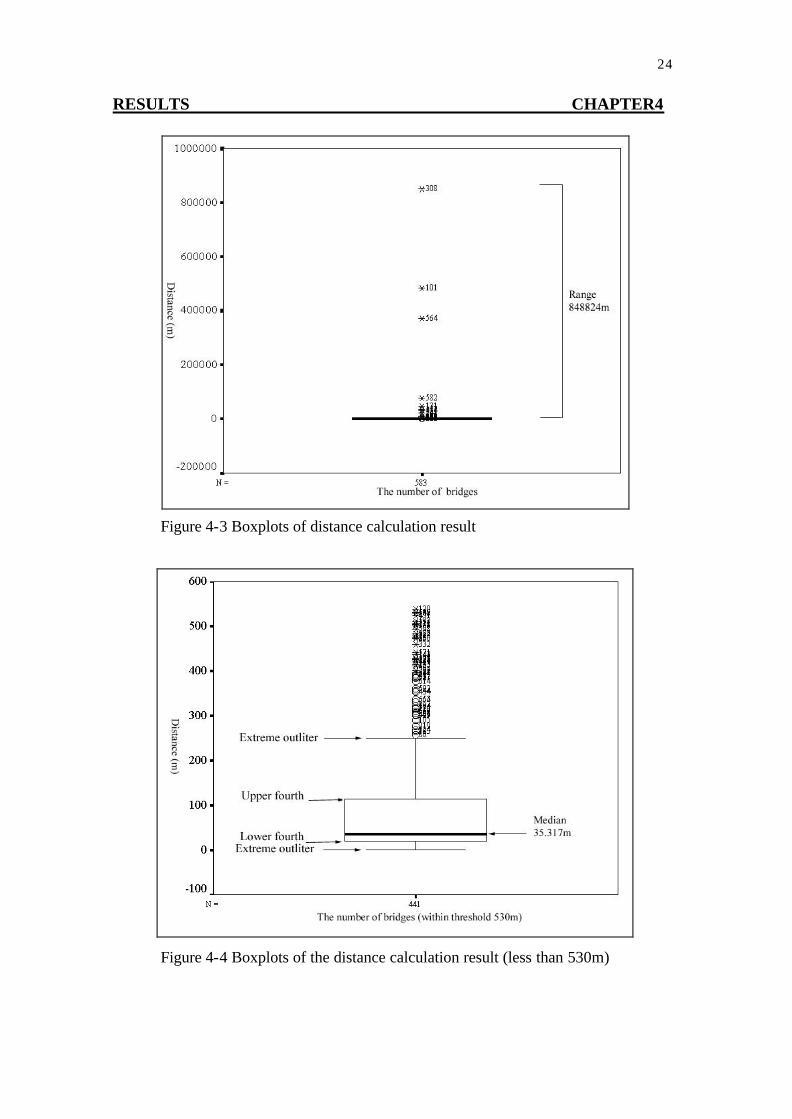
Figure 4-3 and Figure 4-4 show the Boxplots for the result of distance calculation. The range of distance calculation was 848821.2933m (the range of error radius) and the range of bridge length was 997m (the range of error tolerance radius). The range of error radii was too long compare with the range of the error tolerance radii because there were some bridge points had wrong coordinate. A threshold value was necessary to select those bridge points, and not to consider them in the accuracy adjustment.

The median of error radii was considered as the central tendency, the median

was approximately 35.317m. The positional error of the bridge database was quantified with the central tendency (the median of error radii) of the error radii.

24

RESULTS CHAPTER4

Figure 4-3 Boxplots of distance calculation result

Figure 4-4 Boxplots of the distance calculation result (less than 530m)

25

RESULTS CHAPTER4

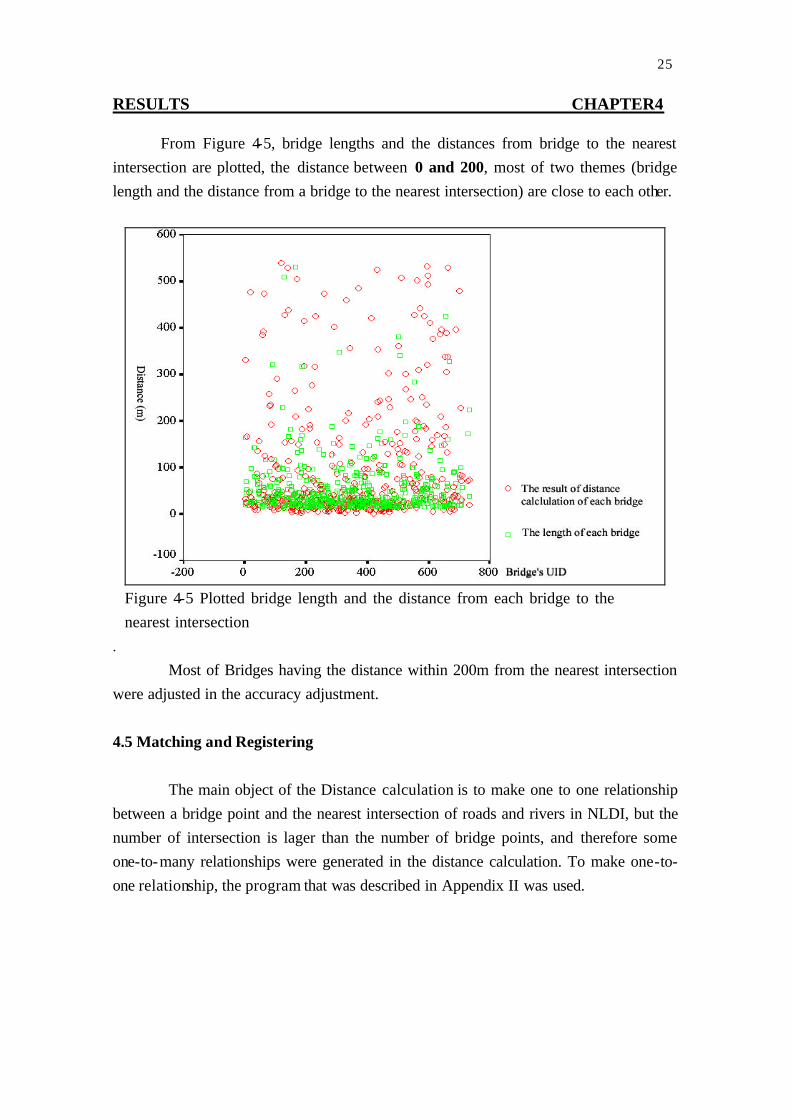
From Figure 4-5, bridge lengths and the distances from bridge to the nearest intersection are plotted, the distance between 0 and 200, most of two themes (bridge length and the distance from a bridge to the nearest intersection) are close to each other.

Figure 4-5 Plotted bridge length and the distance from each bridge to the nearest intersection

.

Most of Bridges having the distance within 200m from the nearest intersection were adjusted in the accuracy adjustment.

4.5 Matching and Registering

The main object of the Distance calculation is to make one to one relationship

between a bridge point and the nearest intersection of roads and rivers in NLDI, but the number of intersection is lager than the number of bridge points, and therefore some one-to-many relationships were generated in the distance calculation. To make one-to- one relationship, the program that was described in Appendix II was used.

26

RESULTS CHAPTER4

Table 4-1 The example of arrangement result of making one-to-one

relationship Uid is the bridge ID number, 1_id and 1_c_dist is the nearest intersection ID

and distance from bridge point to the intersection, 2_id is secondly closest

bridge ID.

Table 4-1 shows an example of the result of the arrangement for one to one relationship. UID 7, 15 and 16 were not matched either because there is no nearest intersection around them or the result of distance calculation is longer than the threshold value (530m). 583 bridge points over river are in the bridge database (Table 2-5), and some of them were abandoned in accuracy adjustment if bridge’s length is longer than the threshold value of bridge lengths, 441 bridge points possessed one-to-one relationship.

4.6 Specifying Error Information in Database

The bridges that did not match with the intersection points in the distance calculation were detected (Table 4-1), and then the result of matching each bridge with the nearest intersection was specified in each record. The distance between a bridge and the nearest intersection was considered as a positional error (error radius), and the bridges that did not match with an intersection, “not matched” was specified in the

27

RESULTS CHAPTER4

result_mat field, and “0” was specified in the 1_id field of not matched intersection (Table 4-2).

Specifying error (1_c_dist in Table 4-2) in the bridge database was a very

important process in accuracy adjustment, because the errors were evaluated in order to decide whether a bridge can be adjusted or not, and it also reduces the uncertainty of the bridge database.

Table 4-2 Specified error and the result of

matching (example) Uid is the bridge id, 1_id is the id of the nearest

intersection, 1_c_dist means the distance from each

bridge to the nearest intersection.

Specifying error process reduced the uncertainty of the bridge database, and the reusability of the bridge database was improved also. The result of error measurement can be basic information of metadata of accuracy

4.7 Accuracy Adjustment by Data Fusion Method

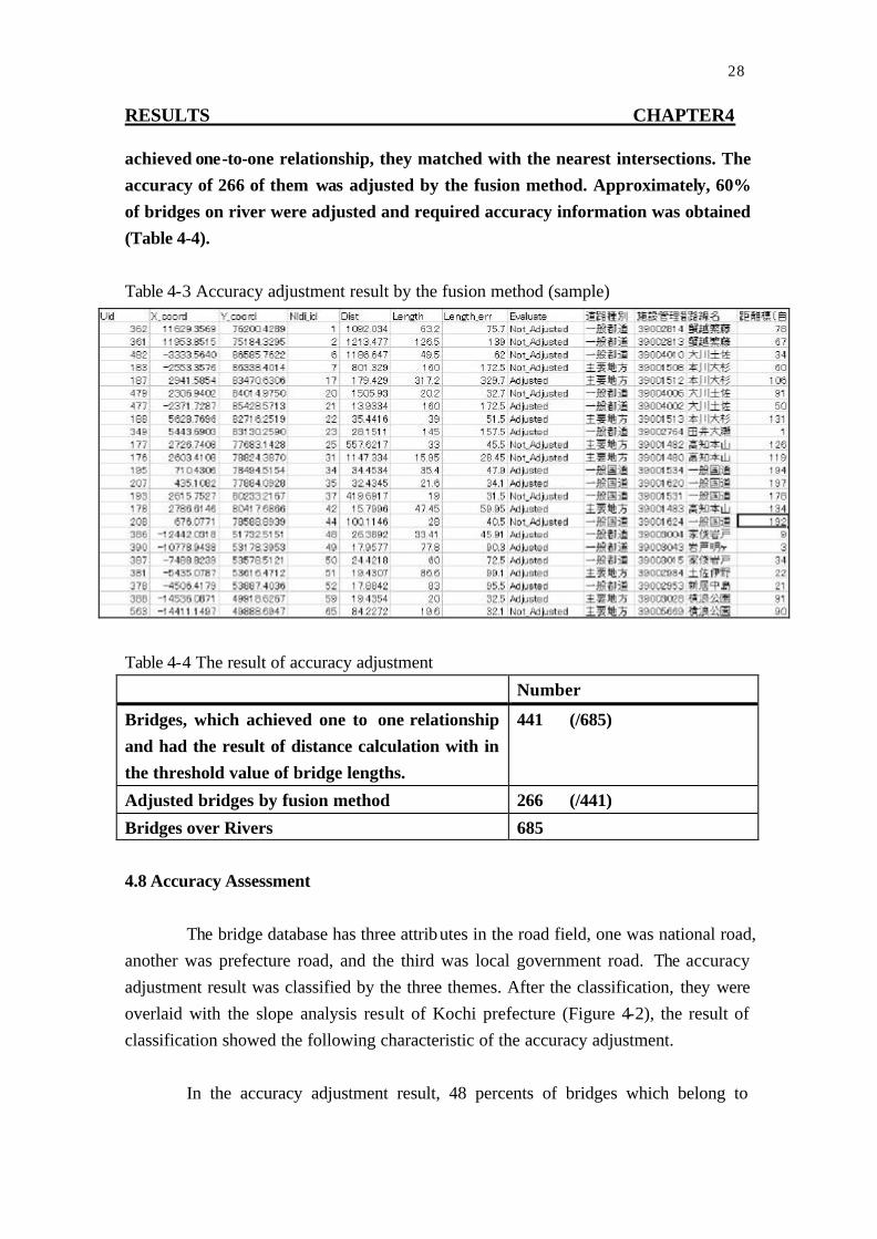
Table 4-3 shows the result of combination between the coordinates of the nearest intersections and the attribute data of the bridge database. 441 bridge points

28

RESULTS CHAPTER4

achieved one-to-one relationship, they matched with the nearest intersections. The accuracy of 266 of them was adjusted by the fusion method. Approximately, 60% of bridges on river were adjusted and required accuracy information was obtained (Table 4-4). Table 4-3 Accuracy adjustment result by the fusion method (sample)

Table 4-4 The result of accuracy adjustment

Number

Bridges, which achieved one to one relationship and had the result of distance calculation with in the threshold value of bridge lengths.

441 (/685)

Adjusted bridges by fusion method 266 (/441)

Bridges over Rivers 685 4.8 Accuracy Assessment

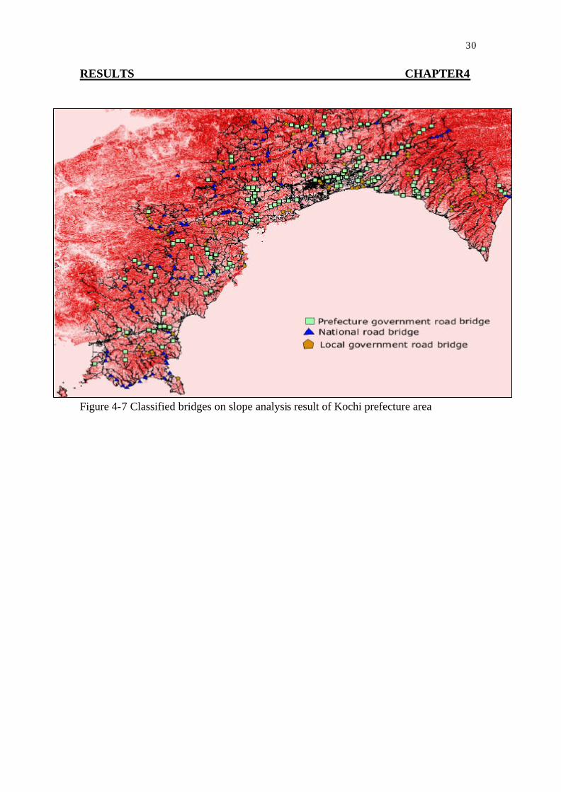
The bridge database has three attributes in the road field, one was national road, another was prefecture road, and the third was local government road. The accuracy adjustment result was classified by the three themes. After the classification, they were overlaid with the slope analysis result of Kochi prefecture (Figure 4-2), the result of classification showed the following characteristic of the accuracy adjustment.

In the accuracy adjustment result, 48 percents of bridges which belong to

29

RESULTS CHAPTER4

national road were adjusted, 69 percents of bridges which belong to prefecture road bridge were adjusted, and 60 percents of bridges which belong to local government road were adjusted.

The reason why the bridges belong to national road have obtained lower

accuracy adjustment result was investigated. Figure 4-6 shows accuracy adjustment result in terms of slope. From the figure, it can be seen that with increasing slope, the number of adjusted bridge decreased. The classification result was overlaid on the slope analysis result of the Kochi prefecture to investigate the relationship between the accuracy adjustment result and slope (Figure 4-6). In Figure 4-7, dark red area is steep slope area and bright pink area is gentle slope area. Most of bridges, which belong to national road were on steep slope area. The reason why national road bridges obtained low accuracy adjustment was they could not be matched with intersection, usually narrow branches of river existed on high slope area, but the NLDI did not have enough resolution to describe small branch, so the intersections on high slope area were not generated, therefore the bridge points that belong to national road could not be adjusted.

Figure 4-6 Accuracy adjustment results in slope

0%

20%

40%

60%

80%

100%

0-5

6-10

11-15

16-20

21-25

26-30

31-35

36-40

more

than

40

slope (degree)

adjustednot_adjusted

30

RESULTS CHAPTER4

Figure 4-7 Classified bridges on slope analysis result of Kochi prefecture area

31 CONCLUSIONS AND SUGGESTION CHAPTER 5

CHAPTER 5 CONCLUSIONS AND SUGGESTION

By the data fusion method, the accuracy of the bridge database was improved.

Modified hierarchy of needs modeling for error modeling in data fusion was introduced for continuous error modeling and adjustment. 60 percents of bridges on rivers took accuracy information from the NLDI. Consusion1. The Accuracy of 60% of Bridges on River were Adjusted by Data Fusion Method

There are some sensitive conditions in the accuracy adjustment by using the data fusion method. Two aspects were mainly considered in the sensitive condition of the accuracy adjustment. Ones are some problems in data fusion method, and the others are the limitations of a test data and reference data in accuracy domain.

Following problems were encountered in the accuracy adjustment by using data fusion method; when the bridge database was converted to a “dbf” file, and when the format (range) of fractional numbers is not defined, some parts of fractional numbers of coordinate and length disappear. And when a field of database imported directly to ArcView program, some part of fractional numbers of coordinate were disappeared. But the disappeared parts were too small number, and they are in the range of error radius, so that they could be ignored. The sensitivity of fractional number in GIS data might be changed according to the accuracy level of a test data. We should take care of the fractional number in GIS. In the distance calculation from each bridge point to the nearest intersection, a lot of one-to-many relationships were generated between bridge points and the intersections in the NLDI, and they prevent accuracy adjustment from making one-to-one relationship. Although the bridges achieved one-to-one relationship, they needed to be evaluated because some of them had mistyping coordinate, therefore the threshold value (530m) was introduced, and they could be arranged by the coded program that was described in Appendix III.

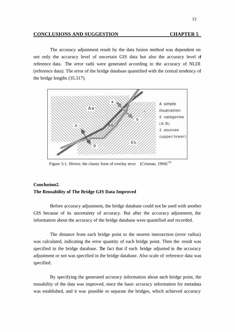
Slivers (Figure 5-1) existed in NLDI, so some intersections need not to be

generated. This problem was handled by comparing an error radius with an error tolerance radius.


The accuracy adjustment result by the data fusion method was dependent on

not only the accuracy level of uncertain GIS data but also the accuracy level of reference data. The error radii were generated according to the accuracy of NLDI (reference data). The error of the bridge database quantified with the central tendency of the bridge lengths (35.317).

Figure 5-1. Slivers: the classic form of overlay error (Crisman, 1994) )13

Conclusion2. The Reusability of The Bridge GIS Data Improved

Before accuracy adjustment, the bridge database could not be used with another GIS because of its uncertainty of accuracy. But after the accuracy adjustment, the information about the accuracy of the bridge database were quantified and recorded.

The distance from each bridge point to the nearest intersection (error radius)

was calculated, indicating the error quantity of each bridge point. Then the result was specified in the bridge database. The fact that if each bridge adjusted in the accuracy adjustment or not was specified in the bridge database. Also scale of reference data was specified.

By specifying the generated accuracy information about each bridge point, the reusability of the data was improved, since the basic accuracy information for metadata was established, and it was possible to separate the bridges, which achieved accuracy


adjustment and not achieved.

Conclusion3. Modified The Hierarchy of Need for Modeling Errors in GIS Was Suggested

When new GIS data, which have road and river information established, the accuracy of the bridge on river can be updated and adjusted continuously. But Veregin (1994)’s the hierarchy of needs for modeling errors was not enough to explain the continuous accuracy adjustment by another reference data. So modified and customized hierarchy of need for modeling errors in GIS was required.

Figure 5-2 Modified hierarchy of need for modeling

errors in GIS

Information updating was not considered in the the Vergin(1994)’s hierarchy of needs for modeling error. After the accuracy adjustment and assessment, the results need to be specified in the database (new step), the step of strategy for error management was needed again in the accuracy adjustment by using the data fusion method (Figure 5-2)

If we obtain another data which can be a reference data in accuracy adjustment


of the bridge database by using data fusion, the accuracy of it can be adjusted and updated continuously, therefore it requires the feedback process between the step of strategy for error management and error measurement (Figure 5-2).

Conclusion4. Successfully the Accuracy Adjustment Result was Assessed by Attribute Data

To assess or to validate the result of accuracy adjustment, the overlay method, surveying data, and such on have been used. In this study, positional accuracy was evaluated by the attribute data of the test data because the accuracy adjustment result strongly depends on the accuracy of the reference data. In the assessment of the accuracy adjustment result, the bridges belong to the national road obtained lowest accuracy adjustment not only because of the accuracy of the bridge database but also because of the limitation of the NLDI. Not only the accuracy of a test data (accuracy unknown GIS data) but also the accuracy of the reference data in an accuracy adjustment by the data fusion method need to be considered. The classified result of accuracy adjustment according to road attribute of the bridge database showed the limitation of the reference data. The reference data used in this study (NLDI) did not have enough resolution for the bridges, which belong to the national road, small branches of rivers or narrow roads were not described in steep slope area in NLDI, some intersections were not generated in steep slop area. Therefore the national road bridge category that has many bridges obtained lower accuracy adjustment result. Conclusion5. Standard data structure and input method required for the data fusion method. In accuracy adjustment and assessment, there was a link data between the bridge database and the intersection of river and road of NLDI, both data have the road attribute information. However the information could not be used as a link data because although the contents of information were same, the character was different. If the characters of the road attributes of the two data were same, the matching, accuracy adjustment and assessment could be done automatically. It is better for Japan Industrial Standards to establish a standard data input method and GIS data structure for GIS data linking and fusion.


Further Study

In accuracy adjustment, the result of the data fusion method strongly depends on the accuracy of reference data. Various data for accuracy adjustment and validation of accuracy adjustment result were needed in using the data fusion method. Unfortunately, the frequency of GIS data updating is quite low, and the speed of establishing GIS data is quite slow. But if it is possible to extract the positions of bridges from high-resolution remote sensing data, those problems will be solved. As further study on the accuracy adjustment of the bridge data by using high-resolution remote sensing data will be investigated.

36 REFERENCES

REFERENNCES 1) Abler, R. F., The National Science Foundation National Center for Geographic

Information and Analysis. International Journal of Geographical Information Systems 1, pp. 305, 1987

2) Accuracy of Spatial Databases, edited by Michael Goodchild and Sucharita Gopal, p1, 1989

3) Giulio Maffini, Michael Arno and Wolfgang Bitterlich, Observation and comments on the generation and treatment of error in digital GIS data. Accuracy of Spatial Databases, M. Goodchild and S. Gopal, Eds. ,Taylor and Francis, Philadelphia, pp. 55, 1989.

4) Goodchild, M. F., Modelling error in objects and fields. Accuracy of Spatial Databases, M. Goodchild and S. Gopal, Eds. ,Taylor and Francis, Philadelphia, pp. 107, 1989.

5) A. Stewart Fotheringham, Scale-independent spatia l analysis. Accuracy of Spatial Databases, M. Goodchild and S. Gopal, Eds., Taylor and Francis, Philadelphia,1989.

6) Giulio Maffini, Michael Arno and Wolfgang Bitterlich, Observation and comments on the generation and treatment of error in digital GIS data. Accuracy of Spatial Databases, M. Goodchild and S. Goopal, Eds. , Taylor and Francis, Philadelphia, pp. 55.

7) Stan Openshaw, “Learning to live with errors of spatial data transformations”, Michael F. Goodchild & Sucharita Gopal (Eds), Accuracy of Spatial Database, 1989.

8) John A. Richards, Xiuping Jia, Remote Sensing Digital Image Analysis, Springer, pp. 305.

9) N. M. Mattikalli. B. J. Devereux and K. S. Richards.” Integration of Remotely Sensed Satellite Images with a Geographical Information System”, Computers & Geosciences Vol.21, No. 8, pp. 947-956,1995.

10) Michael F. Goodchild, “Communicating the Results of Accuracy Assessment: Metadata, Digital Libraries, and Assessing Fitness for use”, Ann Arbor, H. Todd Mowrer & Russell G. Congalton (Eds), Quantifying Spatial Uncertainty in Natural Resources, pp3. 1999.

11) Howard Veregin, Error modeling for the map overlay operation, Michael F. Goodchild & Sucharita Gopal (Eds), Accuracy of Spatial Database, pp.4, 1994.

12) Fred C. Collins and James L. Smith, ”Taxonomy for Error in GIS”, International Symposium on the Spatial Accuracy of Natural Resource Data Base, ASPRS, pp.3, 1994.

37 REFERENCES

13) Nicholas R. Crisman, “Modeling error in overlaid categorical maps”, Michael F. Goodchild & Sucharita Gopal (Eds), Accuracy of Spatial Database, pp.27,1994.

14) Giulio Maffini, Michael Arno and Wolfgang Bitterlich, Observations and comments on the generation and treatment of error in digital GIS data. Michael F. Goodchild & Sucharita Gopal (Eds), Accuracy of Spatial Database, pp.55, 1994.

15) Weldon A. Lodwick, Developing confidence limits on errors of suitability analyses in geographical information systems. Michael F. Goodchild & Sucharita Gopal (Eds), Accuracy of Spatial Database, pp.69,1994

16) Daniel and Griffith, Distance calculation and errors in geographic database. Michael F. Goodchild & Sucharita Gopal (Eds), Accuracy of Spatial Database, 1994

17) Shunji Murai, GIS Work Book, Japan Association of Surveyors, p.35, 1997 18) Michael F. Goodchild(1999), “Communicating the Results of Accuracy Assessment:

Metadata, Digital Libraries, and Assessing Fitness for use”, H. Todd Mowrer & Russell G. Congalton (Eds), Quantifying Spatial Uncertainty in Natural Resources.p.14.

19) H. Todd Mowrer & Russell G. Congalton (Eds), Quantifying Spatial Uncertainty in Natural Resources.p.16 (in introduction),2000.




23) E. Waltz and J. Llinas., Multisensor Data Fusion. Artech House, 1990. 24) Wald L., “Some terms of reference in data fusion”, IEEE Transactions on

Geosciences and Remote Sensing, 37, 3, 1190-1193,1999. 25) Wald L., “Definitions and Terms of Reference in Data Fusion. International

Archives of Photogrammetry and Remote Sensing”, Vol. 32,Part 7-4-3 W6, Valladolid, Spain,3-4 June,1999.

26) Wald L., “A European proposal for terms of reference in data fusion. International Archives of Photogrammetry and Remote Sensing”, Vol. XXXII, Part 7, 651-654, 1998, or Wald L., “Some terms of reference in data fusion”, IEEE Transactions on Geosciences and Remote Sensing, 37, 3, 1190-1193, 1999.

27) L, F. Pau. Sensor data Fusion. Journal of Intelligent and Robotics Systems, vol.1, pp.103-116, 1988.

28) John A. Richards, Xiuping Jia, Remote Sensing Digital Image Analysis, Springer,

39 APPENDIX

APPENDIX I LITERATURE REVIEW

2.1 General

The literatures were reviewed that relate to errors in spatial database, accuracy assessment and adjustment, and also data fusion. 2.2 Accuracy of Spatial Database

2.2.1 Accuracy in GIS Life Cycle

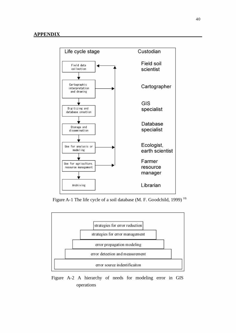
Michael F. Goodchild (1999) )10 explained accuracy in GIS data life cycle (Figure A-1). Accuracy is a dynamic property of the data life cycle. With reference to Figure A-1, changes of data model in the left-hand column, and changes of custodian in the right-hand column, produce the potential for significant changes of accuracy as the current representation is compared to the current reference source.

Life cycle stage of which effective updating after changes in data model, or repeated reassessment of accuracy, can ensure that adequate information on accuracy available to the data’s users. 2.2.2 Hierarchy of Needs for Modeling Error in GIS Operations

Howrd Veregin (1994) )11 established a hierarchy of needs for modeling error in GIS operations (Figure A-2). From the lowest level to the highest level, it has five steps, these are error source identification, error detection and measurement, errors propagation modeling, strategies for error management, and strategies for error reduction. The needs at a specific level must be met before, and individual can progress to higher levels, and if these needs are not met, the attainment of higher levels is retarded or thwarted.

40 APPENDIX

Figure A-1 The life cycle of a soil database (M. F. Goodchild, 1999) )10

Figure A-2 A hierarchy of needs for modeling error in GIS operations

41 APPENDIX

2.2.3 Positional Verses Attribute Errors Positional accuracy is the absolute positional accuracy or the departure in the

geographic location of an object in relation to its location on the ground. Attribute accuracy is concerned with whether attribute that are assigned to feature (points, lines, and polygons) in the GIS are correct and free of bias. By correct we mean that attributes or labels placed on the spatial objects actually correspond to their counterpart on the

ground (Fred C. Collins and James L. Smith, 1992) )12 .

2.2.4 Errors in Overlaid Maps The most common form of error in overlaid maps is called a “sliver”. As

demonstrated in Figure A-3, a simple silver occurs when a boundary between two categories is represented slightly differently in two source maps for the overlay. A small, unintended zone is created. Goodchild (1978) reports that some systems become clogged with the spurious entities that provide evidence of autocorrelations at different levels. These reports are a part of the unwritten lore of GIS, because most agencies are smallest of these, up to the level a user is willing to tolerate (Dougenik, 1980). The availability of the filter makes it important to understand its relation to theory

(Crisman 1994) )13 .

Figure. A-3 Slivers: the classic form of overlay error (Crisman, 1994) )13

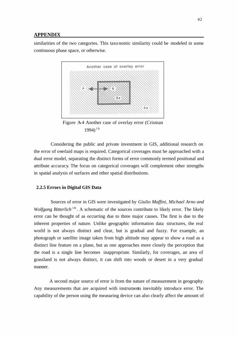
It would be possible to have a feature on one map source which is completely missing on the other, as shown in Figure A-4. While the silver error seems to arise from positional error, such an error is caused by classification and depends on taxonomic

42 APPENDIX

similarities of the two categories. This taxonomic similarity could be modeled in some continuous phase space, or otherwise.

Figure A-4 Another case of overlay error (Crisman

1994) )13

Considering the public and private investment in GIS, additional research on the error of overlaid maps is required. Categorical coverages must be approached with a dual error model, separating the distinct forms of error commonly termed positional and attribute accuracy. The focus on categorical coverages will complement other strengths in spatial analysis of surfaces and other spatial distributions.

2.2.5 Errors in Digital GIS Data Sources of error in GIS were investigated by Giulio Maffini, Michael Arno and

Wolfgang Bitterlich )14 . A schematic of the sources contribute to likely error. The likely error can be thought of as occurring due to three major causes. The first is due to the inherent properties of nature. Unlike geographic information data structures, the real world is not always distinct and clear, but is gradual and fuzzy. For example, an photograph or satellite image taken from high altitude may appear to show a road as a distinct line feature on a plane, but as one approaches more closely the perception that the road is a single line becomes inappropriate. Similarly, for coverages, an area of grassland is not always distinct, it can shift into woods or desert in a very gradual manner.

A second major source of error is from the nature of measurement in geography. Any measurements that are acquired with instruments inevitably introduce error. The capability of the person using the measuring device can also clearly affect the amount of

43 APPENDIX

error introduced. Finally, the scale at which the measurements are made and the frequency of sampling will also introduce potential errors in geographic data.

A third source of error is due to the data models that we use to communicate our measurements. The very structure of the geographic model can be a source of error. In the case of vector, the representation of a line or an edge implies a level of certainty or precision that may not be discernable in the geographic model can be a source of error. In the case of vector, the representation of a line or an edge implies a level of uncertainty or precision that may not be discernable in the real world.

Maffini, Arno & Biotterlich )14 illustrated the size and range of some type of errors generated by GIS users in the digitized process. Simple trials were conducted in order to develop an appreciation of the rage of digitizing errors that can be generated by typical GIS users. The trials were concerned with exploring positional errors. They excluded other types of errors, such as topological problems associated with data base creation.

In the trials an attempt was made to isolate the effects of two factors that one would expect to influence the propagation of error. The first was the scale of the source conducted the digitizing, and the second factor was the speed with which the operator conducted the digitizing. Although efforts were made to be systematic the trials were not scientifically controlled experiments. It is also important to recognize that trial results were based on the digitizing performance of one person.

In the results of digitizing trials, the number of points generated to represent an

entity, and the frequency distribution of error classes for each entity. In the results, it is apparent that the discrete entities, which changes in the scale of the source of the source document used for digitizing, have a more significant impact on positional error than the time taken to digitize.

From the digitizing trials, following conclusions were obtained by Maffini,

Arno & Biotterlich )14 1) Cartographic and digital products should distinguish between judgments

about the interpretation and integration of geographic data. 2) Geographic Information Systems should, and can be used to assess the

44 APPENDIX

consequences of error in geographic data, with GIS tools users will be able to make more informed judgments about the interpretation and integration of geographic data.

3) The design and execution of controlled scientific experiments to determine the error ranges propagated in commonly available geographic data products, a systematic investigation and documentation of these experiments and investigations users could make more informed and appropriate use of the data.

2.2.6 Developing Confidence Limits on Errors of Suitability Analyses in GIS

Confidence limits based on measures of sensitivity are developed for the most widely used types of suitability analyses, weighted intersection overlay and weighted multidimensional scaling. Some underlying types of sensitivity analyses associated with computer map suitability analyses are delineated as a way to construct measures of these delineated sensitivities that in turn become the means by which confidence limits

are obtained. Weldon )15 conducted analyses to obtain confidence limits on errors, which are geographic sensitivity and error propagation analysis and the computational process and mathematical representation of suitability analysis. Two approaches (geographic sensitivity and error propagation analysis, the computational process and mathematical representation of suitability analysis) to confidence limits in the attribute values generated by geographic suitability analyses were developed using suitability measures, attribute sensitivity measures , position sensitivity measures, map removal sensitivity measures, polygon sensitivity measures, and area sensitivity measures

(Weldon A. Lodwick) )15 . 2.2.7 Distance Calculation and Errors in Geographic Database

Daniel and Griffith )16 insisted that we should be compelled to understand the impact of these different sources of error on analytical model before incorporating them as standard options in GIS software. 2.2.8 Separation of Error Into Time Phases

Arnoff(1989) )16 , separates error into time phases and sources (Table A-1).

45 APPENDIX

Table A-1 The separation error into time phases and sources

Stage Sources of Error

Data Collection l Inaccuracies in field measurements l Inaccurate equipment l Incorrect recoding procedures l Errors in the analysis of remotely sensed data

Data Input l Digitizing error l Nature of fuzzy natural boundaries

Data Storage l Numerical precision l Spatial precision ( in raster systems)

Data Manipulation l Wrong class intervals l Boundary errors l Spurious polygons and error propagation with overlay

operation

Data Output l Scaling l Inaccurate output device

Use of Results l Incorrect understanding of information l Incorrect use of data

2.2.9 Separation of Error Into Time Phases

In digital GIS database, there is no scale but resolution, expressed as pixel size (interval or dot per inch), grid cell size or grid interval, ground for satellite images and so on. There is rough relationship between scale and resolution, as follows (Table A-2).

Grid interval = M (scale denominator)/1,000 (meter)

Table A-2. Relationship Between Scale, Accuracy and Resolution (S. Murai, GIS Work

Book) )15 Accuracy Scale Contour Interval (m) Height Accuracy (m) Position Accuracy (m)

1:500 0.5 0.17 0.25

1:1000 1 0.33 0.5 1:2500 2 0.7 1.25

1:5000 5 1.7 2.5

46 APPENDIX

1:10000 10 3 5.0

1:25000 10, 20 3, 7 12.5 2.2.10 Summary

Michael F Goodchild )10 explained how errors should be handled in updating or changing GIS data. Howard vergin )11 introduced a hierarchy of needs for modeling error in GIS operation. Some errors from overlaying digital maps were investigated by

Nicholas R. and Chrisman )13 , including the kinds of errors that types of errors which can arise. It was considered about how to recognize or how to specify the errors in GIS to prevent users from being misled by error prone GIS. In this study, errors in experimental data were investigated in each hierarchy of need for modeling errors for GIS operation. From the investigation, some accuracy adjustment direction and criteria were established. 2.3 Accuracy (Uncertainty) Assessment and Adjustment

2.3.1 Spatial Uncertainty

Spatial uncertainty in attribute values and in position includes accuracy,

statistical precision and bias in initial values, and in estimated predictive coefficients in

statistically calibrated equation of errors (Michael F. Goodchild,1999) )18 . Uncertainty also means different things in different disciplines. For example,

the concept of numerical precision arises from computer science and database management, and refers to the exactness or degree of detail with which an individual observation is measured. Statistical precision refers to the dispersion of repeated observations about their own mean (Quantifying Spatial Uncertainty in Natural

Resources,2000) )19 .

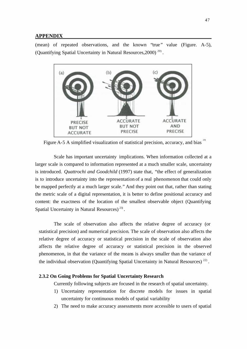
Error may be random or systematic. Random error refers to the difference between and observed value and a predicted or true value (Vogt, 1993). These random deviations are completely the result of chance effects. A common statistic used to describe accuracy is the root mean square error (RMSE), the square root of the quantity, the sum of squares of the errors divided by the number of errors (Slama, 1980). Systematic error, or bias, is the consistent difference between the central tendency

47 APPENDIX

(mean) of repeated observations, and the known “true” value (Figure. A-5),

(Quantifying Spatial Uncertainty in Natural Resources,2000) )20 .

Figure A-5 A simplified visualization of statistical precision, accuracy, and bias

)20

Scale has important uncertainty implications. When information collected at a larger scale is compared to information represented at a much smaller scale, uncertainty is introduced. Quattrochi and Goodchild (1997) state that, “the effect of generalization is to introduce uncertainty into the representation of a real phenomenon that could only be mapped perfectly at a much larger scale.” And they point out that, rather than stating the metric scale of a digital representation, it is better to define positional accuracy and content: the exactness of the location of the smallest observable object (Quantifying

Spatial Uncertainty in Natural Resources) )21 . The scale of observation also affects the relative degree of accuracy (or

statistical precision) and numerical precision. The scale of observation also affects the relative degree of accuracy or statistical precision in the scale of observation also affects the relative degree of accuracy or statistical precision in the observed phenomenon, in that the variance of the means is always smaller than the variance of

the individual observation (Quantifying Spatial Uncertainty in Natural Resources) )22 . 2.3.2 On Going Problems for Spatial Uncertainty Research

Currently following subjects are focused in the research of spatial uncertainty. 1) Uncertainty representation for discrete models for issues in spatial

uncertainty for continuous models of spatial variability 2) The need to make accuracy assessments more accessible to users of spatial

48 APPENDIX

data and model predictions 3) The effect of scale on uncertainty 4) How uncertainty estimates from different disciplines can be combined to

provide a composite estimate of uncertainty in final products.

2.3.3 The Quantification of Positional and Attribute Errors Perhaps the single most compelling reason for the separation of positional and

attribute errors is the difference between the quantification of the two error types. Qualitative attribute errors have traditionally been quantified using an error or confusion matrix (Congalton, 1983, 1991,1993) and (Rosenfield, 1986). Positional errors, however, can be quantified as some true value with an RMS error value (Merchant, 1987). Models for positional accuracy have been developed for points, lines and polygons. Due to the qualitative nature of attribute, no single model has been developed which encompasses both attribute and positional error, but some authors suggest using the Cohen’s Kappa as a method of accuracy comparison (Chrisman,1989).

2.4 Data Fusion

Data fusion research and development were conducted under a wide variety of systems, methods and names. Using recent words such as "data fusion", or "information fusion" translates the recent understanding that whatever the application domain, these synergistic approaches share common problems and

common properties (E. Waltz and J. Llinas.) )23

2.4.1 Definitions and Terms of Data Fusion Terms of reference in information fusion are presented: Merging, Combination

Integration, Concatenation Data assimilation, Optimal Control? Measurements, Signal, Image, Radiances, Reflectance Sample, Pixel, Voxel, Commensurate, Observation, Electronic Imagery, Gray levels, Image Multi-Modality, Multi-Channel, Multi-Band,

Multispectral, and Multi-Frequencies (Wald L.) )24 . It then has been suggested to use the terms like merging and combination in a

49 APPENDIX

much broader sense than fusion, with combination being even broader than merging. These two terms define any process that implies a mathematical operation performed on at least two sets of information. These two terms define any process that implies a mathematical operation performed on at least two sets of information. These definitions are intentionally loose and offer space for various interpretations. Merging or combinations are not defined with opposition to fusion. They are simply more general, also because we often need such terms to describe processes and methods in a general way, without entering details. Integration may play a similar role though it implicitly refers more to concatenation (i.e. increasing the state vector) than to the extraction of

relevant information (Wald L) )25 . Another domain pertains to data fusion: data assimilation or optimal control.

Data assimilation deals with the inclusion of measured data into numerical models for forecasting or analysis of the behavior of a system. A well-known example of a mathematical technique used in data assimilation is the Kalman filtering. Data assimilation is used daily for weather forecasting.

Data fusion may be sub-divided into many domains. For example, the military

community uses the term positional fusion to denote aspects relevant to the assessment of the state vector or identity fusion when establishing the identity of the entities is at stake. If observations are provided by sensors and only by sensors, one will use the term sensor fusion. Image fusion is a sub-class of sensor fusion; here the observations are images. If the support of the information is always a pixel, one may speak of pixel fusion. Other terms easily understandable are measurement fusion, signal fusion, features fusion, and decision fusion. Evidential fusion means that the algorithms behind call upon the evidence theory, etc.

Data fusion is a formal framework in which are expressed the means and tools for the alliance of data originating from different sources. It aims at obtaining information of greater quality; the exact definition of 'greater quality' will depend upon the application. The rationales for proposing this definition are expressed in this

document.（Wald L.） )26 .

2.4.2 Properties of Data Fusion

The properties of information fusion are listed: fusion of attribute, fusion of

50 APPENDIX

analysis and fusion of representations (L, F. Pau.) )27 .

2.4.2.1 Fusion of Attributes Fusion of attributes consists in merging the attributes of a same object, derived

from two representations ( )1(sX t) and ( )2(sX t) at instant t obtained by means of the

sources of information S(1) and S(2), in order to obtain new attributes in the space of sources S=S(1) U S(2).

2.4.2.2 Fusion of Analysis Assume the sources of information are aligned and associated. Fusion of

analysis consists in aggregating representations ( )1(sX t) and ( )2(sX t) , into a new

representation ( )1(sX ) t and ( )2(sX ) t , then in generating an analysis or interpretation of

the object for further use at instant (t+1), or at step i in an iterative process. 2.4.2.3 Fusion of Representations

Fusion of representations is defining and performing meta-operations

applicable to representation ( )1(sX ) t and ( )2(sX ) t , to obtain a new representation

( sX t) . Fusion of representations includes fusion of decisions. This fusion of

representations may be performed at any moment.

2.4.2.4 Data Fusion in Remote Sensing

In remote sensing, data fusion processes, such as classification techniques for mapping, are performed since long, without naming it, and even less looking at it as a concept. According to discussions, remote sensing specialists often say that data fusion is fully illustrated by the merging (the word “combination” can also be used) of images having a higher spatial resolution. Examples are SPOT-XS and P, and Landsat 7-ETM and P. The HIS method is one of the most used method to perform such an operation

51 APPENDIX

(Pohl, Van Genderen 1998). The knowledge-based analysis system developed by Srinivansan and Richards

(1993) is able to analyze the images (Landsat MSS band 5 and 7 and an L band SIR-B synthetic aperture radar image) jointly and thus develop a cover type map that resolves classes that are confused in either the Landsat or radar data alone(John A. Richards,

Xiuping Jia) )28 .

2.4.3 Integration Between Remotely Sensed Data and GIS Data A simple methodology has been developed for raster-to-vector for use in a GIS.

This methodology was employed successfully to integrate both coarse and fine resolution raster image (e.g. LANDSAT MSS and TM; and SPOT HRV) into a vector

GIS. (N. M. Mattikalli. B. J. Devereux and K. S. Richards) )29 .

2.4.4 Summary Frequently the need arises to analyze missed spatial data bases, mixed data sets

consist of satellite spectral, topographic and other points from data. All registered geometrically, as might be found in a GIS. So far, many remotely sensed data were used to merge with other sources for any special purpose. But it is very rare that a GIS data merged with another data. There are advantages of data fusion in GIS, so in this study, data fusion focused on especially GIS data accuracy adjustment.

52 APPENDIX

APPENDIX II

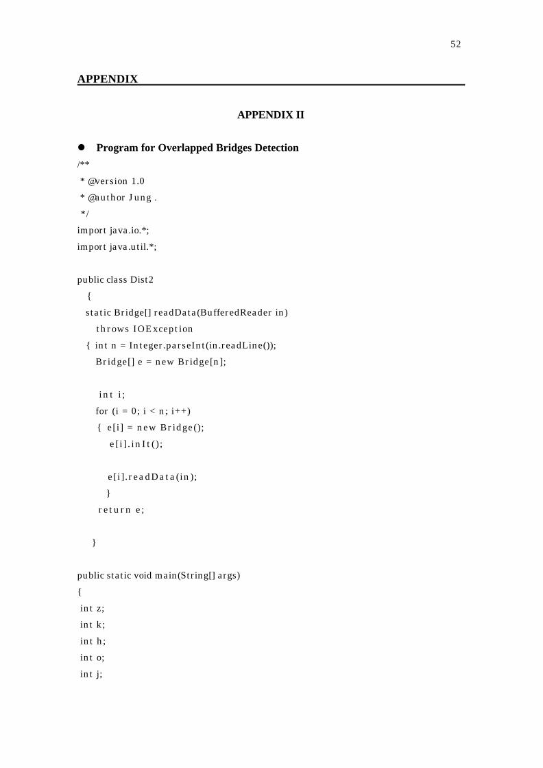
l Program for Overlapped Bridges Detection /**

* @version 1.0

* @author Jung .

*/

import java.io.*;

import java.util.*;

public class Dist2

{

static Bridge[] readData(BufferedReader in)

throws IOException

{ int n = Integer.parseInt(in.readLine());

Bridge[] e = new Bridge[n];

int i ;

for (i = 0; i < n; i++)

{ e[i] = new Bridge();

e[i] . inIt() ;

e[i].readData(in);

}

return e;

}

public static void main(String[] args)

{

int z;

int k;

int h;

int o;

int j;

53 APPENDIX

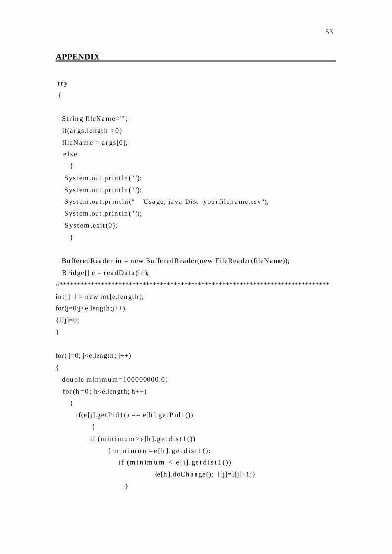
try

{

String fileName="";

if(args.length >0)

fileName = args[0];

else

{

System.out.println("");


System.out.println(" Usage; java Dist yourfilename.csv");


System.exit(0);

}

BufferedReader in = new BufferedReader(new FileReader(fileName));

Bridge[] e = readData(in);

//******************************************************************************

int[] l = new int[e.length];

for(j=0;j<e.length;j++)

{ l[j]=0;

}

for( j=0; j<e.length; j++)

{

double minimum=100000000.0;

for(h=0; h<e.length; h++)

{

if(e[j].getPid1() == e[h].getPid1())

{

if (minimum>e[h].getdist1())

{ minimum=e[h].getdist1() ;

i f (minimum < e[j] .getdist1())

{e[h].doChange(); l[j]=l[j]+1;}

}

54 APPENDIX

}

}

}

for(k=0; k<e.length; k++){

for(o=0; o<l[k];o++)

{


{



{


{



i f (minimum < e[j ] .getdist1())

{ e [ h ] . doChange();

}

}

}

}

}

}

}

for(z=0 ; z< e.length; z++)

{e[z].print();}

//******************************************************************************

in.close();

}

catch(IOException e)

{

System.out.print("Error:" + e);

System.exit(1);

55 APPENDIX

}

}

}

class Bridge{

public Bridge(int bid, int pid1, double dist1)

{

bridge1 = bid;

polyid1 = pid1;

distance1 = dist1;

}

public Bridge(int bid, int pid1, double dist1, int pid2,double dist2, int pid3, double

dist3){

bridge1 = bid;

polyid1 = pid1;

distance1 = dist1;

polyid2 = pid2;

distance2 = dist2;

polyid3 = pid3;

distance3 = dist3;

}

public void doChange(){ polyid1 =polyid2;

p o l y i d 2 = p o l y i d 3 ;

p o l y i d 3 = 0 ;

d i s t a n c e 1 = d i stance2;

d i s tance2 =d i s tance3 ;

d i s t a n c e 3 = 0 . 0 ;

}

public void inIt(){

p o l y i d 1 = 0 ;

56 APPENDIX

p o l y i d 2 = 0 ;

p o l y i d 3 = 0 ;

d i s t a n c e 1 = 0 ;

d i s t a n c e 2 = 0 ;

d i s t a n ce3 =0;

}

public int getPid1(){ return polyid1;}



public double getdist1(){ return distance1;}



public void print(){

System.out.println(bridge1+","+polyid1+","+distance1+","+polyid2+","+distance2+","+p

olyid3+","+distance3);}

public Bridge(){}

public void readData(BufferedReader in) throws IOException

{

String s = in.readLine();

StringTokenizer t = new StringTokenizer(s,",");

bridge1 = Integer.parseInt(t.nextToken());

polyid1 = Integer.parseInt(t.nextToken());

distance1 = Double.parseDouble(t.nextToken());





}

private int bridge1,polyid1,polyid2,polyid3;

private double distance1,distance2,distance3;

}

57 APPENDIX

APPENDIX III

l The program for one to one relationship /**

* @version 1.0

* @author jung .

*/

import java.io.*;

import java.util.*;

public class Dist2

{

static Bridge[] readData(BufferedReader in)

throws IOException

{ int n = Integer.parseInt(in.readLine());

Bridge[] e = new Bridge[n];

int i ;

for (i = 0; i < n; i++)

{ e[i] = new Bridge();

e[i] . inIt() ;

e[i].readData(in);

}

return e;

}

public static void main(String[] args)

{

int z;

int k;

int h;

int o;

int j;

try

{

String fileName="";

if(args.length >0)

58 APPENDIX

fileName = args[0];

else

{



System.out.println(" Usage; java Dist yourfilename.csv");


System.exit(0);

}

BufferedReader in = new BufferedReader(new FileReader(fileName));

Bridge[] e = readData(in);

//******************************************************************************

int[] l = new int[e.length];

for(j=0;j<e.length;j++)

{ l[j]=0;

}


{



{


{

i f ( m i nimum>e[h].getdist1())



{ e [ h ] . d o C h a n g e ( ) ;

l[j]=l[j]+1;}

}

}

}

}

for(k=0; k<e.length; k++){

for(o=0; o<l[k];o++)

59 APPENDIX

{


{



{


{


{ m i nimum=e[h].getdist1();


{ e [ h ] . d o C h a n g e ( ) ;

}

}

}

}

}

}

}

for(z=0 ; z< e.length; z++)

{e[z].print();}

//******************************************************************************

in.close();

}

catch(IOException e)

{

System.out.print("Error:" + e);

System.exit(1);

}

}

}

class Bridge{

public Bridge(int bid, int pid1, double dist1)

{

b r idge1 = bid;

60 APPENDIX

polyid1 = pid1;

distance1 = dist1;

}

public Bridge(int bid, int pid1, double dist1, int pid2,double dist2, int pid3, double

dist3){

bridge1 = bid;

polyid1 = pid1;

distance1 = dist1;

polyid2 = pid2;

distance2 = dist2;

polyid3 = pid3;

distance3 = dist3;

}

public void doChange(){ polyid1 =polyid2;

p o l y i d 2 = p o l y i d 3 ;

p o l y i d 3 = 0 ;



d i s t a n c e 3 = 0 . 0 ;

}

public void inIt(){

p o l y i d 1 = 0;

p o l y i d 2 = 0 ;

p o l y i d 3 = 0 ;

d i s t a n c e 1 = 0 ;

d i s t a n c e 2 = 0 ;

d i s t a n c e 3 = 0 ;

}







public void print(){

61 APPENDIX

System.out.println(bridge1+","+polyid1+","+distance1+","+polyid2+","+

distance2+","+polyid3+","+distance3);}

public Bridge(){}

public void readData(BufferedReader in) throws IOException

{

String s = in.readLine();

StringTokenizer t = new StringTokenizer(s,",");

bridge1 = Integer.parseInt(t.nextToken());







}

private int bridge1,polyid1,polyid2,polyid3;

private double distance1,distance2,distance3;

}

an accuracy adjustment of gis data by using a data fusion ... · school relationship between kut...

Documents