An Academic Response to Basel 3.5

Paul Embrechts1, Giovanni Puccetti2, Ludger Rüschendorf3, Ruodu Wang4, and Antonela Beleraj2

1RiskLab and SFI, Department of Mathematics, ETH Zurich, 8092 Zurich, Switzerland

2School of Economics and Management, University of Firenze, 50127 Firenze, Italy

3Department of Mathematical Stochastics, University of Freiburg, 79104 Freiburg, Germany

4Department of Statistics and Actuarial Science, University of Waterloo, Waterloo, ON N2L3G1, Canada

Abstract

Recent crises in the financial industry have shown weaknesses in the modeling of Risk-Weighted Assets

(RWA). Relatively minor model changes may lead to substantial changes in the RWA numbers. Similar

problems are encountered in the VaR-aggregation of risks. In this article we highlight some of the underlying

issues, both methodologically as well as through examples. In particular we frame this discussion in the

context of two recent regulatory documents we refer to as Basel 3.5.

Keywords: Basel 3.5; Risk-Weighted Assets; Value-at-Risk; Expected Shortfall; model uncertainty; robustness;

backtesting

1 Introduction

In May 2001, the first author contributed to the influential and highly visible Daníelsson et al. (2001). In

their academic response to, at the time, Basel 2 the authors were spot on concerning the weaknesses within the

prevailing, international regulatory framework, as well as for the way in which larger international banks were

managing market, credit and operational risk. We cite from their Executive Summary:

• The proposed regulations fail to consider the fact that risk is endogenous. Value-at-Risk can destabilize

an economy and induce crashes [. . .]

• Statistical models used for forecasting risk have been proven to give inconsistent and biased forecasts,

notably underestimating the joint downside risk of different assets. The Basel Committee has chosen poor

quality measures of risk when better risk measures are available.

• Heavy reliance on credit rating agencies for the standard approach to credit risk is misguided [. . .]

• Operational risk modeling is not possible given current databases [. . .]

• Financial regulation is inherently procyclical [. . .] the purpose of financial regulation is to reduce the

likelihood of systemic crises, these proposals will actually tend to negate, not promote this useful purpose.

1

And as summary:

• Perhaps our most serious concern is that these proposals, taken altogether, will enhance both the pro-

cyclicality of regulation and the susceptibility of the financial system to systemic crises, thus negating the

central purpose of the whole exercise. Reconsider before it is too late.

Unfortunately, five years later it was too late!

The above quotes serve two purposes: first, academia has a crucial role to play in commenting officially

on proposed changes in the regulatory landscape. Second, when well-documented, properly researched and

effectively communicated, we may have an influence on regulatory and industry practice.

For the purpose of this paper, we refer to the regulatory document BCBS (2012) as Basel 3.5 for the trading

book; Basel 4 is already on the regulatory horizon, even if the implementation of Basel 3 is only planned for

2019. In particular, through its consultative document BCBS (2013b), the Basel Committee went already a step

beyond BCBS (2012), indeed "the Committee has its intention to pursue two key confirmed reforms outlined in

the first consultative paper BCBS (2012): stressed calibration [. . .] move from Value-at-Risk (VaR) to Expected

Shortfall (ES)". Our comments are also relevant for insurance regulation’s Solvency 2, now planned in the EU

for January 1, 2016. The Basel 3.5 document arose out of consultations between the regulators, industry and

academia, and this in the wake of the subprime crisis. It also paid attention to and remedied some of the

criticisms raised in Daníelsson et al. (2001); we shall exemplify this below. Among the various issues raised, for

our purpose, the following question (Nr.8, p.41) in BCBS (2012), is relevant:

"What are the likely constraints with moving from Value-at-Risk (VaR) to Expected Shortfall

(ES), including any challenges in delivering robust backtesting and how might these be best

overcome?"

Since its introduction around 1994, VaR has been criticized by numerous academics as well as practitioners

for its weaknesses as the benchmark (see Jorion (2006)) for the calculation of regulatory capital in banking and

insurance:

W1 VaR says nothing concerning the what-if question: "Given we encounter a high loss, what can be said

about its magnitude?";

W2 For high confidence levels, e.g. 95% and beyond, the statistical quantity VaR can only be estimated with

considerable statistical as well as model uncertainty, and

W3 VaR may add up the wrong way, i.e. for certain (one-period) risks it is possible that

VaRα(X1 + · · ·+Xd) > VaRα(X1) + · · ·+ VaRα(Xd) ; (1.1)

the latter defies the (better said, some) notion of diversification.

The worries W1-W3 were early on brushed aside as being less relevant for practice. By now practice has caught

up and W1-W3 have become highly relevant, whence parts of Basel 3.5.

2

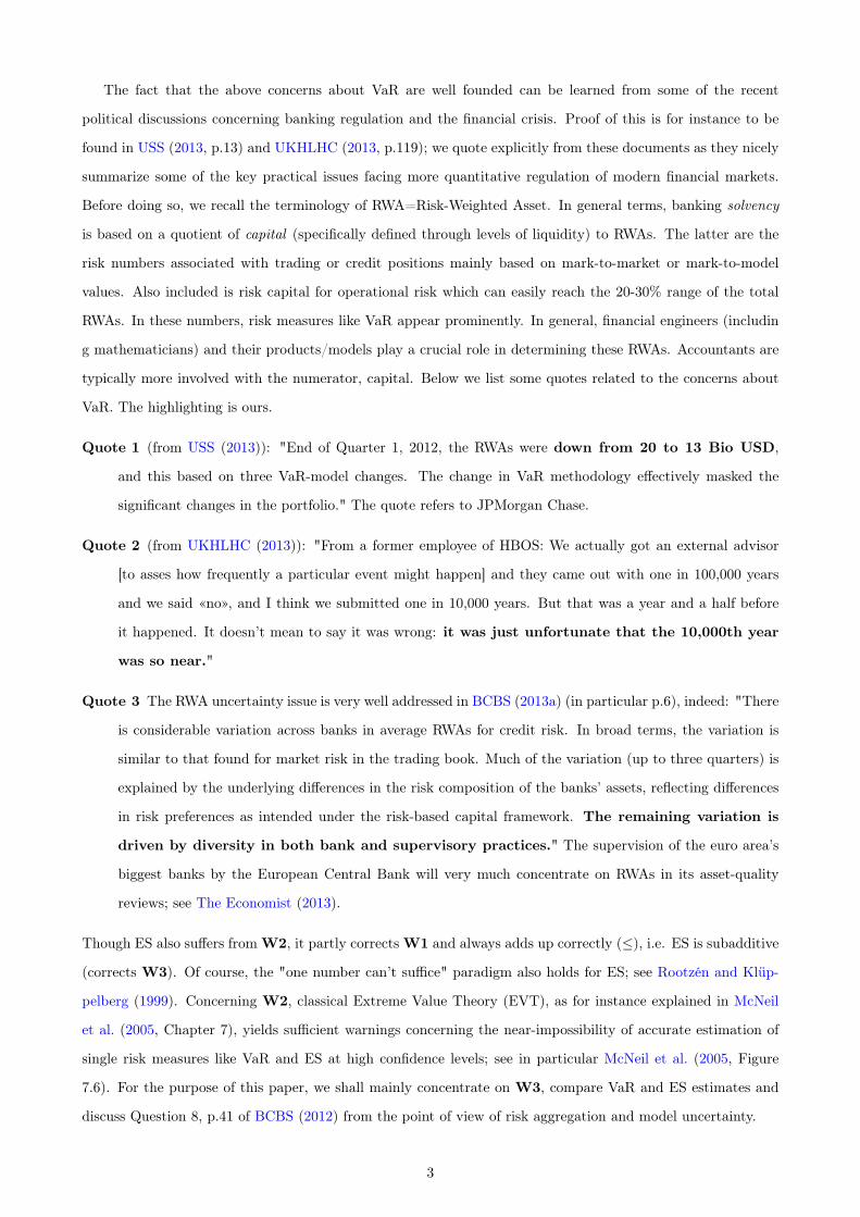
The fact that the above concerns about VaR are well founded can be learned from some of the recent

political discussions concerning banking regulation and the financial crisis. Proof of this is for instance to be

found in USS (2013, p.13) and UKHLHC (2013, p.119); we quote explicitly from these documents as they nicely

summarize some of the key practical issues facing more quantitative regulation of modern financial markets.

Before doing so, we recall the terminology of RWA=Risk-Weighted Asset. In general terms, banking solvency

is based on a quotient of capital (specifically defined through levels of liquidity) to RWAs. The latter are the

risk numbers associated with trading or credit positions mainly based on mark-to-market or mark-to-model

values. Also included is risk capital for operational risk which can easily reach the 20-30% range of the total

RWAs. In these numbers, risk measures like VaR appear prominently. In general, financial engineers (includin

g mathematicians) and their products/models play a crucial role in determining these RWAs. Accountants are

typically more involved with the numerator, capital. Below we list some quotes related to the concerns about

VaR. The highlighting is ours.

Quote 1 (from USS (2013)): "End of Quarter 1, 2012, the RWAs were down from 20 to 13 Bio USD,

and this based on three VaR-model changes. The change in VaR methodology effectively masked the

significant changes in the portfolio." The quote refers to JPMorgan Chase.

Quote 2 (from UKHLHC (2013)): "From a former employee of HBOS: We actually got an external advisor

[to asses how frequently a particular event might happen] and they came out with one in 100,000 years

and we said «no», and I think we submitted one in 10,000 years. But that was a year and a half before

it happened. It doesn’t mean to say it was wrong: it was just unfortunate that the 10,000th year

was so near."

Quote 3 The RWA uncertainty issue is very well addressed in BCBS (2013a) (in particular p.6), indeed: "There

is considerable variation across banks in average RWAs for credit risk. In broad terms, the variation is

similar to that found for market risk in the trading book. Much of the variation (up to three quarters) is

explained by the underlying differences in the risk composition of the banks’ assets, reflecting differences

in risk preferences as intended under the risk-based capital framework. The remaining variation is

driven by diversity in both bank and supervisory practices." The supervision of the euro area’s

biggest banks by the European Central Bank will very much concentrate on RWAs in its asset-quality

reviews; see The Economist (2013).

Though ES also suffers from W2, it partly corrects W1 and always adds up correctly (≤), i.e. ES is subadditive

(corrects W3). Of course, the "one number can’t suffice" paradigm also holds for ES; see Rootzén and Klüp-

pelberg (1999). Concerning W2, classical Extreme Value Theory (EVT), as for instance explained in McNeil

et al. (2005, Chapter 7), yields sufficient warnings concerning the near-impossibility of accurate estimation of

single risk measures like VaR and ES at high confidence levels; see in particular McNeil et al. (2005, Figure

7.6). For the purpose of this paper, we shall mainly concentrate on W3, compare VaR and ES estimates and

discuss Question 8, p.41 of BCBS (2012) from the point of view of risk aggregation and model uncertainty.

3

2 How much superadditive can VaR be?

In Embrechts et al. (2013), the question is addressed how large the gap between the left- and right-hand

side in (1.1) can be. The answer is very much related to the issue of model uncertainty (MU), especially at the

level of inter-dependence, i.e. dependence uncertainty.

Let us first recall the standard definitions of VaR and ES. Suppose X is a random variable (rv) with

distribution function (df) FX , FX(x) = P(X ≤ x) for x ∈ R. For 0 ≤ α < 1, we then define

VaRα(X) = F−1X (α) = inf{x ∈ R : FX(x) > α}, (2.1)

and

ESα(X) =1

1− α

∫ 1

α

VaRβ(X)dβ.

Whenever FX is continuous, it follows that

ESα(X) = E[X|X > VaRα(X)],

leading to the standard interpretation for ES as a conditional expected loss. The ES and its equivalence in the

continuous setting, are known under different names and abbreviations such as TVaR, CVaR, CTE, TCE and

AVaR. When discrete distributions are involved, the above cited notions are not more equivalent; see Acerbi and

Tasche (2002). Throughout the paper also let VaR1(X) = F−1X (1) = inf{x ∈ R : FX(x) = 1} be the essential

supremum of the support of X.

Our set-up is as follows.

• Suppose X1, . . . , Xd are one-period risk positions with dfs Fi, i = 1, . . . , d, also denoted as Xid∼ Fi.

We assume F1, . . . , Fd to be known for the purpose of our discussion. In practice this may correspond

to models fitted to historical data, or models chosen in a stress-testing environment. One could also

envisage empirical dfs when sufficient data are available. Important is that in the analyses and examples

below we disregard statistical uncertainty; this can, and should be added in a full-scale discussion. As a

consequence, for the purpose of this paper MU should henceforth be interpreted as functional-MU at the

level of inter-dependence rather than statistical-MU. Full MU would combine (at least) both.

• Consider the portfolio position X+d = X1 + · · · + Xd. The techniques discussed below would also

allow for the analysis of other portfolio structures like for instance X∨d = max(X1, . . . , Xd), X∧d =

min(X1, . . . , Xd) or X+d 1{X∨

d >m} for some m > 0, typically large. MU results for such more general

examples however need further detailed study; see Embrechts et al. (2013) for some remarks on this.

• Denote by VaRα(Xi), i = 1, . . . , d, the marginal VaRs at the common confidence level α ∈ (0, 1), typically

close to 1. For the moment we concentrate on VaR as a risk measure, as it still is the regulatory benchmark.

Other risk measures will appear later in the paper.

4

Task: Calculate VaRα(X+d ).

As stated, this task cannot be performed since for the calculation of VaRα(X+d ) we need a joint model for the

random vector X = (X1, . . . , Xd)′. Under a specific joint model, the calculation of VaRα(X+

d ) amounts to a

d-dimensional integral (or sum in the discrete case). Only in very few cases this can be done analytically. As

a consequence numerical integration and/or Monte Carlo methodology, including the use of quasi-random (low

discrepancy) techniques, may enter. For α close to 1, tools from rare event simulation become important; see for

instance Asmussen and Glynn (2007) (Chapter VI). For a more geometric approach, useful in lower dimensions,

say d ≤ 5, see Arbenz et al. (2011, 2012).

When we relax from a full joint distributional assumption (a single model) to a specific subclass of models,

it may be possible to obtain some inequalities or asymptotics (in α → 1 or d → ∞, say) for VaRα(X+d ). For

instance, if X is elliptically distributed, then

VaRα(X+d ) ≤

d∑i=1

VaRα(Xi);

see McNeil et al. (2005, Theorem 6.8). An important subclass of elliptical distributions form the so-called

multivariate normal variance mixture models, i.e.

X d= µ+

√WAZ,

where

(i) Z ∼ Nk(0, Ik), Ik stands for the k-dimensional identity matrix;

(ii) W ≥ 0 is a non-negative, scalar-valued rv which is independent of Z, and

(iii) A ∈ Rd×k and µ ∈ Rd.

See McNeil et al. (2005, Section 3.2) for this definition. For the most general definition based on affine trans-

formations of spherical random vectors, see McNeil et al. (2005, Section 3.3.2). In many ways, elliptical models

are like "heaven" for finance and risk management; see McNeil et al. (2005, Theorem 6.8 and Proposition 6.13).

Unfortunately, and this in particular in moments of stress, the world of finance may be highly non-elliptical.

A further interesting class of models results for X comonotonic, i.e. there exist increasing functions ψi,

i = 1, . . . , d, and an rv Z so that

Xi = ψi(Z) a.s., i = 1, . . . , d,

and in that case

VaRα(X+d ) =

d∑i=1

VaRα(Xi); (2.2)

i.e. VaR is comonotone additive. For a proof of (2.2), see McNeil et al. (2005, Theorem 6.15). Recall that

two risks (two rvs) with finite second moments are comonotone exactly when the joint model achieves maximal

correlation, typically less than 1; see McNeil et al. (2005, Theorem 5.25). Consequently, strictly superadditive

5

risks, like in (1.1), correspond to dependence structures with less than maximal correlation. This often leads to

confusion amongst practitioners; it was also one of the reasons (a correlation pitfall) for writing Embrechts et al.

(2002). Without extra model knowledge, we are hence led to calculating best-worst VaR bounds for VaRα(X+d )

in the presence of dependence uncertainty:

VaRα(X+d ) = inf{VaRα(XF

1 +· · ·+XFd ) : X = (XF

1 , . . . , XFd )

′has joint df F with marginals F1, . . . , Fd}, (2.3)

VaRα(X+d ) = sup{VaRα(XF

1 +· · ·+XFd ) : X = (XF

1 , . . . , XFd )

′has joint df F with marginals F1, . . . , Fd}. (2.4)

The terminology, best versus worst, of course very much depends on the situation at hand: whether one is long

or short in a trading environment or whether the bounds are interpreted by a regulator or a bank, say.

We further comment on notation: recall that the only available information so far are the marginal distri-

butions of the risks, i.e. Xid∼ Fi, i = 1, . . . , d. Whenever we use a joint distribution function F with those

given marginals for the vector X, we denote X+d = XF

1 + · · · + XFd in order to highlight this choice; see (2.3)

and (2.4) above. We hope that the reader is fine with this slight abuse of notation.

Using the notion of copula we may rephrase (2.3) and (2.4) by applying Sklar’s Theorem; see McNeil et al.

(2005, Theorem 5.3). Denote by Cd the set of all d-dimensional copulas, then (2.3) and (2.4) are equivalent to:

VaRα(X+d ) = inf{VaRα(XC

1 + · · ·+XCd ) : C ∈ Cd, Xi

d∼ Fi, i = 1, . . . , d}, (2.5)

VaRα(X+d ) = sup{VaRα(XC

1 + · · ·+XCd ) : C ∈ Cd, Xi

d∼ Fi, i = 1, . . . , d}. (2.6)

As with F above, the upper C-index highlights the fact that the joint df of (X1, . . . , Xd)′ is F = C(F1, . . . , Fd).

Rewriting the optimization problem (2.3)-(2.4) in its equivalent copula form (2.5)-(2.6) stresses the fact that,

once we are given the marginal dfs Fi, i = 1, . . . , d, solving for VaR and VaR amounts to finding the copulas

which, together with the F ′i s, achieve these bounds. Hence, solving for (2.3)-(2.4), or equivalently for (2.5)-(2.6)

(the set-up we will usually consider) one obtains the MU-interval for fixed marginals:

VaRα(X+d ) ≤ VaRα(X+

d ) ≤ VaRα(X+d ). (2.7)

If an inequality in (2.7) becomes an equality for a given copula C, the corresponding copula C is referred to as an

optimal coupling. A current important area of research corresponds to finding the bounds in (2.7), analytically

and/or numerically, prove sharpness under specific conditions and find the corresponding optimal couplings.

The interval[VaRα(X+

d ),VaRα(X+d )]yields a measure for MU across all possible joint models as a function

of inter-dependencies between the marginal factors (recall that we assume the F ′is to be known!). So far, we

assume no prior knowledge about the inter-dependence among the marginal risks X1, . . . , Xd. If extra, though

still incomplete information, like for instance "all Xi’s are positively correlated" is available, then the above

MU interval narrows. An important question becomes: can one quantify such MU? This is precisely the topic

treated in Embrechts et al. (2013); Bignozzi and Tsanakas (2013); Barrieu and Scandolo (2013). There is a

6

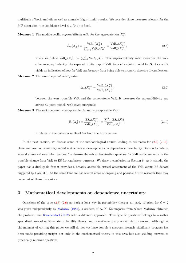
multitude of both analytic as well as numeric (algorithmic) results. We consider three measures relevant for the

MU discussion; the confidence level α ∈ (0, 1) is fixed.

Measure 1 The model-specific superadditivity ratio for the aggregate loss X+d :

4α(X+d ) =

VaRα(X+d )∑d

i=1 VaRα(Xi)=

VaRα(X+d )

VaR+α (X+

d ), (2.8)

where we define VaR+α (X+

d ) :=∑di=1 VaRα(Xi). The superadditivity ratio measures the non-

coherence, equivalently, the superadditivity gap of VaR for a given joint model for X. As such it

yields an indication of how far VaR can be away from being able to properly describe diversification.

Measure 2 The worst superadditivity ratio:

4α(X+d ) =

VaRα(X+d )

VaR+α (X+

d ); (2.9)

between the worst-possible VaR and the comonotonic VaR. It measures the superadditivity gap

across all joint models with given marginals.

Measure 3 The ratio between worst-possible ES and worst-possible VaR:

Bα(X+d ) =

ESα(X+d )

VaRα(X+d )

=

∑di=1 ESα(Xi)

VaRα(X+d )

; (2.10)

it relates to the question in Basel 3.5 from the Introduction.

In the next section, we discuss some of the methodological results leading to estimates for (2.3)-(2.10);

these are based on some very recent mathematical developments on dependence uncertainty. Section 4 contains

several numerical examples. Section 5 addresses the robust backtesting question for VaR and comments on the

possible change from VaR to ES for regulatory purposes. We draw a conclusion in Section 6. As it stands, the

paper has a dual goal: first it provides a broadly accessible critical assessment of the VaR versus ES debate

triggered by Basel 3.5. At the same time we list several areas of ongoing and possible future research that may

come out of these discussions.

3 Mathematical developments on dependence uncertainty

Questions of the type (2.3)-(2.6) go back a long way in probability theory: an early solution for d = 2

was given independently by Makarov (1981), a student of A. N. Kolmogorov from whom Makarov obtained

the problem, and Rüschendorf (1982) with a different approach. This type of questions belongs to a rather

specialized area of multivariate probability theory, and is mathematically non-trivial to answer. Although at

the moment of writing this paper we still do not yet have complete answers, recently significant progress has

been made providing insight not only in the mathematical theory in this area but also yielding answers to

practically relevant questions.

7

To investigate problems with dependence uncertainty like (2.3)-(2.6), it is useful to define the set of all

possible aggregations:

Sd = Sd(F1, . . . , Fd) = {X1 + · · ·+Xd : X1d∼F1, . . . , Xd

d∼Fd}.

Such problems lead to research on the probabilistic properties of and statistical inference in this set Sd (Sd was

formally introduced in Bernard et al. (2013a), but all prior research in this area dealt in some form or another

with the same framework). For example, the questions (2.3)-(2.4) can be rephrased as

VaRα(X+d ) = inf

S∈Sd

VaRα(S) and VaRα(X+d ) = sup

S∈Sd

VaRα(S). (3.1)

A full characterization of Sd is still out of reach; recently however, significant progress has been made, especially

in the so-called homogeneous case. We refer to a recent book Rüschendorf (2013) for an overview of research

on extremal problems with marginal constraints and dependence uncertainty. In particular, the book provides

links between (2.3)-(2.6) and copula theory, mass-transportation and financial risk analysis.

The homogeneous case

Let us first look at the case F1 = · · · = Fd =: F , which we call a homogeneous model. For this model,

analytical results are available. Analytical values for VaRα(X+d ) have been obtained in Wang et al. (2013)

and Puccetti and Rüschendorf (2013) for the homogeneous model when the marginal distributions have a tail-

decreasing density (such as Pareto, Gamma or Lognormal distributions). Wang et al. (2013) also provide

analytical expressions for VaRα(X+d ) for marginal distributions with a decreasing density. These results are

summarized below.

Proposition 3.1 (Corollary 3.7 of Wang et al. (2013), in a slightly different form). Suppose that the density

function of F is decreasing on [β,∞) for some β ∈ R. Then, for α ∈ [F (β), 1) and X d∼F ,

VaRα(X+d ) = dE[X|X ∈ [F−1(α+ (d− 1)cd,α), F−1(1− cd,α)]], (3.2)

where cd,α is the smallest number in [0, (1− α)/d] such that

∫ 1−c

α+(d−1)cF−1(t)dt ≥ 1− α− dc

d(F−1(α+ (d− 1)c) + F−1(1− c)). (3.3)

Moreover, suppose that the density function of F is decreasing on its support. Then for α ∈ (0, 1) and X d∼F ,

VaRα(X+d ) = max{(d− 1)F−1(α) + F−1(0), dE[X|X ≤ F−1(α)]}. (3.4)

Although the expressions (3.2)-(3.4) look somewhat complicated, they can be reformulated using the notion

of duality which dates back to Rüschendorf (1982), and the resulting dual representation originated in the theory

8

of mass-transportation. The following proposition provides an equivalent representation of (3.2). It is stated

in Puccetti and Rüschendorf (2013), in a slightly modified form and under a more general condition of complete

mixability.

Proposition 3.2. Under the same assumptions of Propostion 3.1, suppose that for any sufficiently large thresh-

old s it is possible to find a < s/d such that

D(s) :=d∫ baF (x)dx

(b− a)= F (a) + (d− 1)F (b), (3.5)

where b = s− (d− 1)a, with F−1(1−D(s)) ≤ a. Then, for α ≥ 1−D(s) we have that

VaRα(X+d ) = D−1(1− α). (3.6)

The proof of Propositions 3.1 and 3.2 are based on the recently introduced and further developed mathe-

matical concept of complete mixability.

Definition 3.1 (Wang and Wang (2011)). The marginal distribution F is said to be d-completely mixable if

there exist rvs X1, . . . , Xd with df F such that X1 + · · ·+Xd is almost surely constant.

Recent results on complete mixability are summarized in Wang and Wang (2011) and Puccetti et al. (2012);

an earlier study on the problem of constant sums can be found in Rüschendorf and Uckelmann (2002), with

ideas that originated from the early 80’s (see Rüschendorf (2013)). A necessary and sufficient condition for

distributions with monotone densities to be completely mixable is given in Wang and Wang (2011); it is used

in the proof of the bounds in Propositions 3.1 and 3.2.

Complete mixability, as opposed to comonotonicity, corresponds for this problem to extreme negative de-

pendence. In other words, VaR is obtained through a concept of extreme negative correlation (given that

correlation exists) between conditional distributions, instead of maximal correlation as discussed in Section

2. This rather counter-intuitive mathematical observation partially answers why VaR is non-subadditive, and

warns that regulatory or pricing criteria based on comonotonicity are not as conservative as one may think.

So far, conditional complete mixability and hence sharpness of the dual bound for VaRα(X+d ) has only been

shown for dfs satisfying the tail-decreasing density condition of Proposition 3.1. Of course, this condition is

satisfied by most distributional models used in risk management practice. For such models we are hence able

to calculate (3.1), ∆α(X+d ) and Bα(X+

d ) as defined in (2.9) and (2.10). Examples will be given later.

Towards the inhomogeneous case

When the assumption of homogeneity F1 = · · · = Fd is removed, analytical results become much more

challenging to obtain. The connection between (3.1) and the concept of convex order turns out to be relevant.

Relations between the two concepts were described in Bernard et al. (2013a, Theorem 4.6) and Bernard et al.

(2013b, Theorem 2.4 and Appendix (A1)–(A4)). Let F [α]i be the conditional distribution of Fi on [F−1i (α),∞)

9

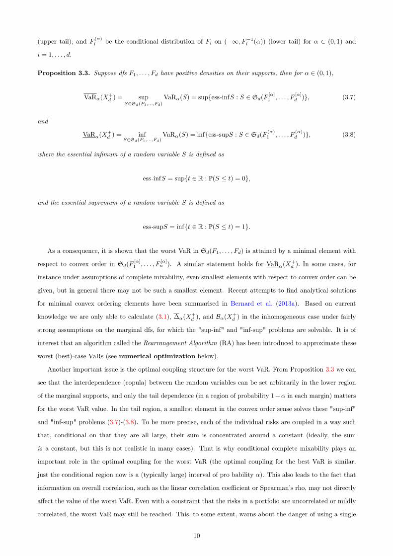
(upper tail), and F(α)i be the conditional distribution of Fi on (−∞, F−1i (α)) (lower tail) for α ∈ (0, 1) and

i = 1, . . . , d.

Proposition 3.3. Suppose dfs F1, . . . , Fd have positive densities on their supports, then for α ∈ (0, 1),

VaRα(X+d ) = sup

S∈Sd(F1,...,Fd)

VaRα(S) = sup{ess-infS : S ∈ Sd(F[α]1 , . . . , F

[α]d )}, (3.7)

and

VaRα(X+d ) = inf

S∈Sd(F1,...,Fd)VaRα(S) = inf{ess-supS : S ∈ Sd(F

(α)1 , . . . , F

(α)d )}, (3.8)

where the essential infimum of a random variable S is defined as

ess-infS = sup{t ∈ R : P(S ≤ t) = 0},

and the essential supremum of a random variable S is defined as

ess-supS = inf{t ∈ R : P(S ≤ t) = 1}.

As a consequence, it is shown that the worst VaR in Sd(F1, . . . , Fd) is attained by a minimal element with

respect to convex order in Sd(F[α]1 , . . . , F

[α]n ). A similar statement holds for VaRα(X+

d ). In some cases, for

instance under assumptions of complete mixability, even smallest elements with respect to convex order can be

given, but in general there may not be such a smallest element. Recent attempts to find analytical solutions

for minimal convex ordering elements have been summarised in Bernard et al. (2013a). Based on current

knowledge we are only able to calculate (3.1), ∆α(X+d ), and Bα(X+

d ) in the inhomogeneous case under fairly

strong assumptions on the marginal dfs, for which the "sup-inf" and "inf-sup" problems are solvable. It is of

interest that an algorithm called the Rearrangement Algorithm (RA) has been introduced to approximate these

worst (best)-case VaRs (see numerical optimization below).

Another important issue is the optimal coupling structure for the worst VaR. From Proposition 3.3 we can

see that the interdependence (copula) between the random variables can be set arbitrarily in the lower region

of the marginal supports, and only the tail dependence (in a region of probability 1−α in each margin) matters

for the worst VaR value. In the tail region, a smallest element in the convex order sense solves these "sup-inf"

and "inf-sup" problems (3.7)-(3.8). To be more precise, each of the individual risks are coupled in a way such

that, conditional on that they are all large, their sum is concentrated around a constant (ideally, the sum

is a constant, but this is not realistic in many cases). That is why conditional complete mixability plays an

important role in the optimal coupling for the worst VaR (the optimal coupling for the best VaR is similar,

just the conditional region now is a (typically large) interval of pro bability α). This also leads to the fact that

information on overall correlation, such as the linear correlation coefficient or Spearman’s rho, may not directly

affect the value of the worst VaR. Even with a constraint that the risks in a portfolio are uncorrelated or mildly

correlated, the worst VaR may still be reached. This, to some extent, warns about the danger of using a single

10

number as dependence indicator in a quantitative risk management model. In the recent paper Bernard et al.

(2013b), it has been shown that additional variance constraints may lead to essentially improved VaR bounds.

Numerical optimization

Numerical methods are regarded as very useful when it comes to optimization problems. One such method

is the rearrangement algorithm (RA) introduced in Puccetti and Rüschendorf (2012b) which was modified,

extended and further discussed with applications to quantitative risk management in Embrechts et al. (2013).

The RA is a simple but fast algorithm designed to approximate convex minimal elements in a set Sd through

discretization. The RA allows for a fast and accurate computation of the bounds in (3.1) for arbitrary marginal

dfs, both in the homogeneous as well as inhomogeneous case. The method uses a discretization step of the

relevant quantile region (N = 106, say) resulting in a N × d matrix on which, through successive operations, a

matrix with minimal variance for the row-sums (think of complete mixability) is obtained. The RA can easily

handle large dimensionality problems of d ≈ 1000, say. For details and examples, see Embrechts et al. (2013). As

argued in ?, the numerical approximations obtained through the RA suggest that the bound VaR in Proposition

3.1 is sharp for all commonly used marginal distributions, and this without the requirement of a tail-decreasing

density. Up to now, we do not have a formal proof of this. In Bernard et al. (2013b), an extension of the RA –

called ERA – is introduced and shown to give reliable bounds for the variance constrained VaR.

Asymptotic equivalence of worst VaR and worst ES

For any random variable Y , VaRα(Y ) is bounded above by ESα(Y ). As a consequence the worst case VaR

is bounded above by the worst case ES, i.e.

VaRα(X+d ) ≤ ESα(X+

d ) (3.9)

Since ESα(X+d ) =

∑di=1 ESα(Xi), (3.9) gives a simple way to calculate upper bounds of the worst VaR. This

bound implies that

Bα(X+d ) =

ESα(X+d )

VaRα(X+d )≥ 1. (3.10)

It was an observation made in Puccetti and Rüschendorf (2012c) that the bound in (3.9) is asymptotically sharp

under general conditions, i.e. an asymptotic equivalence of worst VaR and worst ES holds.

The exact identity of worst-possible VaR and ES estimates holds for bounded homogeneous portfolios when

the common marginal distribution is completely mixable, as indicated in the following remark.

Remark 3.1. Assume that F is a bounded, continuous distribution on the bounded interval [F−1(α), b], b >

F−1(α). Assume also that F is d-completely mixable in [F−1(α), b], i.e. there exists a random vector (X∗1 , . . . , X∗d )′

and a constant k such that

P (X∗1 + · · ·+X∗d = k |X∗i ∈ [F−1(α), b], 1 ≤ i ≤ d) = 1.

11

By the definition of VaR in (2.1), we then have that

VaRα(X∗1 + · · ·+X∗d ) = k, (3.11)

and

k = E

[d∑i=1

X∗i |X∗i ∈ [F−1(α), b], 1 ≤ i ≤ d

]=

d∑i=1

ESα(X∗i ) = ESα(X∗1 + · · ·+X∗d ). (3.12)

Because of (3.9), equations (3.11) and (3.12) imply

VaRα(X∗1 + · · ·+X∗d ) = ESα(X∗1 + · · ·+X∗d ).

The above example suggests a strong connection between VaRα(X+d ) and ESα(X+

d ). Indeed, consider (3.7),

and note that by the definition of F [α]i , ESα(X+

d ) = E[S] for any S ∈ Sd(F[α]1 , . . . , F

[α]d ). So mathematically,

the link between VaRα(X+d ) and ESα(X+

d ) really concerns the difference between ess-infS and E[S] for some

S in Sd(F[α]1 , . . . , F

[α]d ). Intuitively, such S which solves the "sup-inf" and "inf-sup" problems should have a

rather small value of |S −E[S]|, leading to a small value of |VaRα(X+d )−ESα(X+

d )|. Also, the cd,α = 0 case in

Proposition 3.1 points in the same direction.

The asymptotic equivalence of worst VaR and worst ES was established in Puccetti and Rüschendorf (2012c)

in the homogeneous case based on the dual bounds in Embrechts and Puccetti (2006) and an assumption of

conditional complete mixability. The following extension to some class of inhomogeneous models was given

in Puccetti et al. (2013, Theorem 4.2) based on new sufficient condition to complete mixability.

Proposition 3.4 (Asymptotic equivalence of worst VaR and ES). Given a set of m marginal distributions

F1, . . . , Fm, assume that, for any i ∈ N,

Xid∼ Fj for some j ∈ {1, . . . ,m}.

Assume also that Fj has a finite, positive mean and is continuous with a continuous and positive density on

[F−1j (α), F−1j (1)]. Then for α ∈ (0, 1) we have, as d→∞, that

Bα(X+d ) =

ESα(X+d )

VaRα(X+d )→ 1. (3.13)

The assumptions of the positive density and the continuity of the marginals in Proposition 3.4 were later

removed in Wang and Wang (2013). A notion of asymptotic mixability (asymptotically constant sum) implies

the asymptotic equivalence of worst VaR and worst ES (see Puccetti and Rüschendorf (2012a); Bernard et al.

(2013b)), indicating that this equivalence is connected with the law of large numbers and can be expected under

general conditions on the marginal distributions. The equivalence (3.13) is also suggested by several numerical

examples (see Examples 4.1 and 4.2 in Section 4).

Remark 3.2. An immediate consequence from (3.13) is that in the finite mean, homogeneous case, when

12

VaRα(X1) > 0, as d→∞, we have that

4α(X+d ) =

VaRα(X+d )

VaR+α (X+

d )→ ESα(X1)

VaRα(X1). (3.14)

Generally speaking, the worst superadditivity ratio 4α(X+d ) is asymptotically ESα(X+

d )/VaR+α (X+

d ) in all

homogeneous and inhomogeneous models of practical interest. In other words, we can say that the worst VaR

is almost as extreme as the worst ES for d large. It is worth pointing out that the worst superadditivity ratio

4α(X+d ) approaches infinity when ESα(X+

d ) is infinite; this is consistent with (3.14) and was shown in Puc-

cetti and Rüschendorf (2012c). Models leading to (estimated) infinite mean risks have attracted considerable

attention in the literature; see for instance the early contribution Nešlehová et al. (2006) within the realm of

operational risk and Delbaen (2009) for a more methodological point of view. Clearly, ES is not defined in this

case, nor does there exist any non-trivial coherent risk measure on the space of infinite mean rvs; see Delbaen

(2009). As a consequence, as VaR is always well-defined, it may become a risk measure of "last resort". We

shall not enter into a more applied "pro versus contra" discussion on the topic here, but just stress the extra

insight our results give within the context of Basel 3.5. In particular, note that for infinite mean risks the worst

VaR grows much faster than the comonotonic one.

Remark 3.3. So far we have mainly looked at the asymptotic properties when the portfolio dimension d becomes

large, i.e. d→∞, like in Proposition 3.4. Alternatively, one could consider d fixed and α ↑ 1. The latter then

quickly becomes a question in (Multivariate) Extreme Value Theory ; indeed for α close to 1 one is concerned

about the extreme tail-behavior of the underlying dfs. The reader interested in results of this type can for

instance consult Mainik and Rüschendorf (2012) and Mainik and Embrechts (2013) and the references therein.

Finally, one could also consider joint asymptotic behavior d = d(α) where both d → ∞ and α ↑ 1 together in

a coupled way; this would correspond to so-called Large Deviations Theory ; see Asmussen and Glynn (2007,

Section VI) for an introduction in the context of rare event simulation.

4 Examples

By (3.14), the ratio between the ES and the VaR of a random variable represents a degree of superadditivity

which is peculiar to its distribution: it measures how badly VaR can behave in a homogeneous model. We

start computing the ES/VaR ratio in some homogeneous examples F1 = . . . = Fd and later discuss some

inhomogeneous examples.

The Pareto case

Suppose Xid∼ Pareto(θ), i = 1, . . . , d, i.e.

1− Fi(x) = P (Xi > x) = (1 + x)−θ, x ≥ 0. (4.1)

13

Power-laws of the type (4.1) are omnipresent in finance and insurance, often with θ values in the range [0.5, 5];

see Embrechts et al. (1997, Chapter 6). The lower range [0.5,1] typically corresponds to catastrophe insurance,

the upper one, [3,5], to market return data. Operational risk data typically spans the whole range, and indeed

beyond; see Moscadelli (2004) and Gourier et al. (2009).

Under (4.1) we have that for θ > 0, α ∈ (0, 1),

VaRα(Xi) = (1− α)−1/θ − 1,

and for θ > 1, α ∈ (0, 1),

ESα(Xi) =θ

θ − 1VaRα(Xi) +

1

θ − 1.

As a consequence, we have that for i = 1, . . . , d,

ESα(Xi)

VaRα(Xi)=

θ

θ − 1+

1

(θ − 1)VaRα(Xi).

As the Pareto distribution (4.1) is unbounded from above, the latter equation implies that

limα↑1

ESα(Xi)

VaRα(Xi)=

θ

θ − 1> 1. (4.2)

Result (4.2) holds true if we replace the exact Pareto df in (4.1) by a so-called power-tail-like df, i.e.

1− F (x) = (1 + x)−θL(x),

where L is a so-called slowly varying function in Karamata’s sense; see McNeil et al. (2005, Definition 7.7). For

fast decaying tails, like in the normal case, the limit in (4.2) equals 1, so that for α close to 1, there is not much

difference between using Value-at-Risk or Expected Shortfall as a basis for risk capital calculations. In the case

of Pareto tails, the difference can however be substantial. In Tables 1– 3 we illustrate values for the ES/VaR

ratio for Pareto, Lognormal and Exponential distributions. Combined with (3.14), for α close to 1, these results

already yield a fast, rough estimate for ∆α(X+d ) for d large. For example, in the case of the above Pareto(θ) df

with θ = 2, from (3.14) and (4.2) we expect values ∆α(X+d ) ≈ 2, as Table 1 confirms.

α θ = 1.1 θ = 1.5 θ = 2 θ = 3 θ = 4

0.99 11.154337 3.097350 2.111111 1.637303 1.4874920.995 11.081599 3.060242 2.076091 1.603135 1.4540800.999 11.018773 3.020202 2.032655 1.555556 1.405266α→ 1 11.000000 3.000000 2.000000 1.500000 1.333333

Table 1: Values for the ES/VaR ratio for Pareto(θ) distributions.

14

α θ = 0.5 θ = 1 θ = 1.5 θ = 2 θ = 2.5

0.99 1.200364 1.487037 1.920334 2.621718 3.8585990.995 1.184949 1.443519 1.823195 2.415980 3.4152420.999 1.158988 1.372433 1.670393 2.107238 2.787941α→ 1 1.000000 1.000000 1.000000 1.000000 1.000000

Table 2: Values for the ES/VaR ratio for LogN(0, θ) distributions.

α θ = 0.5 θ = 1 θ = 1.5 θ = 2 θ = 2.5

0.99 1.217147 1.217147 1.217147 1.217147 1.2171470.995 1.188739 1.188739 1.188739 1.188739 1.1887390.999 1.144765 1.144765 1.144765 1.144765 1.144765α→ 1 1.000000 1.000000 1.000000 1.000000 1.000000

Table 3: Values for the ES/VaR ratio for Exponential(θ) distributions.

Some numerical examples

Example 4.1 (the homogeneous case)

We start with an example which is realistic in the context of operational risk under the Basel 2 guidelines;

see for instance McNeil et al. (2005, Chapter 10). Indeed, internal operational risk data often show Pareto-type

behavior; see for instance Moscadelli (2004); Gourier et al. (2009). The values of d used typically correspond

either to d = 8 business lines or d = 56 = 8 × 7 (7 being the standard number of risk types). For α we take

the Basel 2 value 0.999. The numbers in Table 4 were calculated with the theory summarized in Section 3 for

homogeneous Pareto(2) portfolios; they speak for themselves. Also note that the numerical values reported are

very much in line with the asymptotics as presented in (3.13) and (3.14) together with (4.2), and this already for

small (d = 8) to moderate values (d = 56) of d. Also note that in this Pareto example, the VaR-MU spread is

much larger than the ES-MU spread, suggesting that ES is "more robust" than VaR with respect to dependence

uncertainty. We want to stress that often, in industry, VaRα(X+d ) is reported as the capital upper bound for

operational risk within the Loss Distribution Approach (LDA). "Diversification arguments" are then used in

order to obtain a 10 to 30 % deduction. In Table 4 (d = 8) this leads to a capital charge of around 170 to 220,

the worst possible VaR however being 465. In this case, the results reported in Section 3 tell us that the full

VaR-range [31, 465] is attainable (given that all marginal dfs are Pareto(2)); more research is needed concerning

the question "which interdependencies (copulas) yield VaR values in the superadditivity range [245, 465]". We

will comment on this question in Section 5. For the moment it suffices to understand that statements like

"diversification yields" have to be taken with care; financial institutions indeed need to carefully explain where

such diversification deductions come from.

This is not just an academic issue; for instance, FINMA, the Swiss regulator, ordered UBS to increase its

capital reserves against litigation, compliance and operational risks by 50%. Financial Times (2013) reports

that: "FINMA’s move, which UBS expects will increase its risk-weighted assets [RWAs] by SFr 28 bn." Banks

15

d=8 VaRα ESα VaR+α VaRα ESα 4α(X+

d ) Bα(X+d )

31 178 245 465 498 1.898 1.071

d=56 VaRα ESα VaR+α VaRα ESα 4α(X+

d ) Bα(X+d )

53 472 1715 3454 3486 2.014 1.009

Table 4: Values (rounded) for best- and worst VaR and ES for a homogeneous portfolio with d Pareto(2) risks;α = 0.999. VaR+

α represents VaR in the comonotonic case. Comonotonic values might not be strict multiplesbecause of rounding.

worldwide are carefully monitored by their respective regulatory authorities concerning the calculation of RWAs

in general, and operational risk in particular. This is no doubt due to the aftermath of the subprime crisis,

the LIBOR scandal and the allegations around possible manipulations of the USD 4 tn global foreign exchange

market. Regulators are in general also worried by some of the complexity of RWA models in use in the industry

and the possibly resulting model uncertainty and/or regulatory arbitrage.

Example 4.2 (an inhomogeneous portfolio)

In Table 5 we present an inhomogeneous portfolio in line with Proposition 3.4. We have three types of

marginal dfs, Pareto(2), Exponential(1) and Lognormal(0,1), yielding dimensions d = 3k for k = 1, 3, 10, 20. In

particular, note the line for Bα(X+d ) with values close to 1 as k (hence d) increases, as stated in (3.13). Again

note that values of Bα(X+d ) close to 1 are already reached for small to moderate values of d. One could compare

and contrast the numbers more in detail or include other dfs/parameters. The main point however is that,

using the results reported in Section 3 and the RA, these numbers can actually be calculated ; see for instance

the recent paper Aas and Puccetti (2013) where the RA is applied to a real bank’s portfolio.

k=1 VaRα ESα VaR+α VaRα ESα 4α(X+

d ) Bα(X+d )

31 64 60 77 100 1.2833 1.299

k=3 VaRα ESα VaR+α VaRα ESα 4α(X+

d ) Bα(X+d )

31 107 179 277 301 1.5475 1.087

k=10 VaRα ESα VaR+α VaRα ESα 4α(X+

d ) Bα(X+d )

36 190 595 979 1003 1.6454 1.025

k=20 VaRα ESα VaR+α VaRα ESα 4α(X+

d ) Bα(X+d )

71 264 1190 1982 2006 1.6655 1.012

Table 5: Values (rounded) for best- and worst VaR and ES for a inhomogeneous portfolio divided into 3homogeneous subgroups i.e. d = 3k having marginals distributed as F1=Pareto(2), F2=Exp(1), F3=LogN(0,1);α = 0.999. Comonotonic values might not be strict multiples because of rounding.

16

5 Robust backtesting of risk measures

Finally, we want to further comment on Question Nr.8 from BCBS (2012): whereas it is fully clear that,

if one wants to regulate a financial institution relying on a number, ES is better than VaR concerning W1

and W3. However, both suffer from W2. In Section 3, and the examples in Section 4, we have seen that

under a worst scenario of interdependence, both VaR and ES yield similar values. Backtesting VaR is fairly

straightforward (hit-and-miss tests) whereas for ES one has to assume an underlying model; for an EVT-based

approach, see for instance McNeil et al. (2005, p. 168). Below, we will make the latter statement scientifically

more precise.

If one for instance needs to compare different backtesting procedures on one measure, the situation for

ES as compared to VaR is less favorable. The relevant notion here is elicitability ; see Gneiting (2011). Such

forecasts, in our case risk measures like VaR and ES, are functionals of the underlying data: they map a

data vector to a real number, in some cases an interval. A (statistical) functional is called elicitable if it can

be defined as the minimizer of a suitable, strictly convex scoring function. The scoring functions are then

used to compare competing forecasts through their average scores calculated from point forecast and realized

observations. In Gneiting (2011) it is shown that in general VaR is elicitable whereas ES is not. To this

observation, the author adds the following statement: "The negative result [for ES] may challenge the use

of the CVaR [ES] functional as a predictive measure of risk, and may provide a partial explanation for the

lack of literatu re on the evaluation of CVaR forecasts, as opposed to quantile or VaR forecasts." Recently,

considerable progress has been made concerning the embedding of the statistical theory of elicitability within

the mathematical theory of risk measures; see for instance Ziegel (2013). An interesting question that early on

emerged from this research was: "Do there exist (non-trivial) coherent (i.e. subadditive) risk measures which are

elicitable?" A positive answer is to be found in Ziegel (2013) and Bellini and Bignozzi (2013): the τ -expectiles.

The τ -expectile, 0 < τ < 1, for an rv X with E[X2] <∞ is defined as

eτ (X) = argminx∈RE[τ max(X − x, 0)2 + (1− τ) max(x−X, 0)2

].

It is the unique solution x of the equation

τE[max(X − x, 0)] = (1− τ)E[max(x−X, 0)].

For τ = 1/2, e1/2(X) = E[X]. One can show that for 0 < τ < 1, eτ is elicitable; for 1/2 ≤ τ < 1, eτ is

subadditive, whereas for 0 < τ ≤ 1/2, eτ is superadditive. Moreover, eτ is not comonotone additive. In Bellini

and Bignozzi (2013) it is shown that, under a standard technical condition, the only elicitable and coherent risk

measures are the expectiles. We are not advocating eτ as the risk measure to use, but mainly want to show

the kind of research which is triggered by parts of Basel 3.5. For more information, see for instance Bellini

et al. (2013) and Delbaen (2013). Early contributions are to be found in Rémillard (2013) (Section 4.4.4.1).

We do mention the above publications as on p.60 in BCBS (2012) it is mentioned that "Spectral risk measures

17

are a promising generalization of ES that is cited in the literature." As mentioned above, it is shown that

non-trivial law-invariant spectral risk measures such as ES are not elici table. As a consequence, and this by

definition of elicitability, "objective comparison and backtesting of competing estimation procedures for spectral

risk measures is difficult, if not impossible, in a decision theoretically sound manner"; see Discussion in Ziegel

(2013). The latter paper also describes a possible approach to ES-prediction. Clearly, proper backtesting of

spectral risk measures needs more research.

A different way of looking at the relative merits of VaR and ES as measures of financial risk is presented

in Davis (2013). In the latter paper, the author uses the notion of prequential statistics and concludes: "The

point [. . .] is that significant conditions must be imposed to secure consistency of mean-type estimates [ES], in

contrast to the situation for quantile estimates [VaR] (Theorem 5.2) where almost no conditions are imposed.

[. . .] This seems to indicate – in line with the elicitability conclusions – that verifying the validity of mean-based

estimates is essentially more problematic than the same problem for quantile-based statistics." To what extent

these conclusions tip the decision from an ES-based capital charge back to a VaR-based one is at the moment

not yet clear.

Whereas the picture concerning backtesting across risk measures needs further discussion, the situation

becomes even more blurred when a notion of robustness is added. In its broadest sense, robustness has to

do with (in)sensitivity to underlying model deviations and/or data changes. Also here, a whole new field of

research is opening up; at the moment it is difficult to point to the right approach. The quotes and the references

below give the interested reader some insight on the underlying issues and different approaches. The spectrum

goes from a pure statistical one, like in Huber and Ronchetti (2009), to a more economics decision making

one, like Hansen and Sargent (2007). In the former text, robustness mainly concerns so-called distributional

robustness: what are the consequences when the shape of the actual underlying distribution deviates slightly

from the assumed model. In the latter text, the emphasis lies more on robust control, in particular, how should

agents cope with fear of model misspecification, and goes back to earlier work in statistics, mainly Whittle

(1983) (the first edition appeared already in 1963). The authors of Hansen and Sargent (2007) provide the

following advice: "If Peter Whittle wrote it, read it." Finally, an area of research, that also uses the term

robustness and is highly relevant in the context of Section 3, is the field of Robust Optimization as for instance

summarized in Ben-Tal et al. (2009).

The main point of the comments above is that "there is more to robustness than meets the eye". In many

ways, in some form or another, robustness lies at the core of financial and insurance risk management. Below

we gathered some quotes on the topic which readers may find interesting to follow-up; we briefly add a comment

when relevant in the light of our paper as presented so far.

Quote 1 (from Kou et al. (2013)): "Coherent risk measures are not robust". The authors champion Median

Shortfall, defined in an obvious manner. This measure was for instance used in the analysis of operational

risk data in Moscadelli (2004). Note however that Median Shortfall is a VaR at a higher confidence level.

Quote 2 (from Stahl (2009)): "Use stress testing based on mixture models [. . .] contamination." In practice

18

one often uses so-called contamination; this amounts to model constructions of the type (1 − ε)F + εG

with 0 < ε < 1 and ε typically small. In this case, the df F corresponds to "normal" behavior whereas G

corresponds to a stress component. In Stahl (2009) this approach is also championed and embedded in a

broader Bayesian Ansatz.

Quote 3 (from Cont et al. (2010)) "Our results illustrate in particular, that using recently proposed risk

measures such as CVaR/Expected Shortfall leads to a less robust risk measurement procedure than Value-

at-Risk."

Quote 4 (from Cambou and Filipović (2013)) "ES is robust, and VaR is non-robust based on the notion of

φ-divergence."

Quote 5 (from Krätschmer et al. (2013)) "We argue here that Hampel’s classical notion of quantitative ro-

bustness is not suitable for risk measurement and we propose and analyse a refined notion of robustness

that applies to tail-dependent law-invariant convex risk measures on Orliz spaces."

First of all, the reference to "Hampel’s classical notion" is in line with the more statistical approach to

robustness, as presented in Huber and Ronchetti (2009). Second, these authors introduce an index of

quantitative robustness. As a consequence, and this somewhat in contrast to Quotes 1 and 3: "This

new look at robustness will then help us to bring the argument against coherent risk measures back into

perspective: robustness is not lost entirely but only to some degree when VaR is replaced by a coherent

risk measure such as ES."

The above quotes hopefully bring the robustness in "robust backtesting" somewhat into perspective. More

discussions with regulators are needed in order to understand what precisely is intended when formulating this

aspect of future regulation. As we already stressed, the multi-facetted notion of robustness must be key to any

financial business and consequently regulation. In its broadest interpretation as "resilience against or awareness

of model and data sensitivity" this ought to be clear to all involved. How to make this awareness more tangible

is a key task going forward.

6 Conclusion

The recent financial crises have shown how unreliably some quantitative tools perform in stormy markets.

Through its Basel 3.5 documents BCBS (2012) and BCBS (2013a), the Basel Committee has opened up the

discussion in order to make the international banking world a safer place for all involved. Admittedly, our

contribution to the choice of risk measure for the potential supervision of market risk is only a minor one and

only touches upon a small aspect of the above regulatory documents. We do however hope that some of the

methodology, examples and research reviews presented will contribute to a better understanding of the issues at

hand. On some of the issues, our views are clear, like "In the finite mean case, ES is a superior risk measure to

VaR in the sense of aggregation and answering the crucial what-if question". The debate for the lack of proper

19

aggregation has been known to academia since VaR was introduced around 1994: in several, for practice, relevant

case s VaR adds up wrongly, whereas ES always adds up correctly (subadditivity). More importantly, thinking

in ES-terms makes risk managers concentrate more on the "what-if" question, whereas the VaR thinking is

only concerned about the "if" question. However, in the infinite mean case ES cannot be used, yet we have a

complete toolkit available to handle VaR in a reliable way. Moreover, in the finite mean case our results show

that quite generally the conservative estimates provided by ES are roughly not too pessimistic if compared

to the corresponding VaR estimates in the worst case dependence scenarios. Both however remain statistical

quantities, the estimation of which is marred by model risk and data scarcity. The frequency rather than severity

thinking is also very much embedded in other fields of finance; think for instance of the calibrations used by

rating agencies for securitization products (recall the (in)famous CDO senior equity tranches) or companies

(transition and default probabilities). Backtesting models to data remains a crucial aspect throughout finance;

elicitability and prequentist forecasting add new aspects to this discussion. Robustness remains, for the moment

at least, somewhat elusive. Our brief review of some of the recent work, and this motivated by Basel 3.5, will

hopefully entice more academic as well as practical research and discussions on these very important themes.

Acknowledgement

The authors would like to thank RiskLab and the Forschungsinstitut für Mathematik (FIM) at the Depart-

ment of Mathematics of the ETH Zurich for its hospitality and financial support while carrying out research

related to this paper. Paul Embrechts also acknowledges financial support by the Swiss Finance Institute.

Ruodu Wang acknowledges financial support from the FIM and the Natural Sciences and Engineering Research

Council of Canada (NSERC) during his visit to ETH Zurich.

References

Aas, K. and G. Puccetti (2013). Bounds for total economic capital: the DNB case study. Preprint, University

of Firenze.

Acerbi, C. and D. Tasche (2002). On the coherence of expected shortfall. J. Bank. Financ. 26 (7), 1487 – 1503.

Arbenz, P., P. Embrechts, and G. Puccetti (2011). The AEP algorithm for the fast computation of the distri-

bution of the sum of dependent random variables. Bernoulli 17 (2), 562–591.

Arbenz, P., P. Embrechts, and G. Puccetti (2012). The GAEP algorithm for the fast computation of the

distribution of a function of dependent random variables. Stochastics 84 (5-6), 569–597.

Asmussen, S. and P. W. Glynn (2007). Stochastic Simulation: Algorithms and Analysis, Volume 57. New York:

Springer.

Barrieu, P. and G. Scandolo (2013). Assessing financial model risk. Preprint, LSE.

20

BCBS (2012). Consultative Document May 2012. Fundamental review of the trading book. Basel Committee on

Banking Supervision. Basel: Bank for International Settlements.

BCBS (2013a). Regulatory consistency assessment programme (RCAP) – Analysis of risk-weighted assets for

market risk. Basel Committee on Banking Supervision. Basel: Bank for International Settlements.

BCBS (2013b). Consultative Document October 2013. Fundamental review of the trading book: A revised market

risk framework. Basel Committee on Banking Supervision. Basel: Bank for International Settlements.

Bellini, F. and V. Bignozzi (2013). Elicitable risk measures. Preprint, ETH Zurich.

Bellini, F., B. Klar, A. Müller, and E. R. Gianin (2013). Generalized quantiles as risk measures. Preprint,

University of Milano Bicocca.

Ben-Tal, A., L. El Ghaoui, and A. Nemirovski (2009). Robust optimization. Princeton, NJ: Princeton University

Press.

Bernard, C., X. Jiang, and R. Wang (2013a). Risk aggregation with dependence uncertainty. Insurance Math.

Econom., to appear.

Bernard, C., L. Rüschendorf and S. Vanduffel (2013b). Value-at-Risk bounds with variance constraints. Preprint,

University of Freiburg.

Bignozzi, V. and A. Tsanakas (2013). Model uncertainty in risk capital measurement. Preprint, ETH Zurich.

Cambou, M. and D. Filipović (2013). Scenario aggregation for solvency regulation. Preprint, EPF Lausanne.

Cont, R., R. Deguest, and G. Scandolo (2010). Robustness and sensitivity analysis of risk measurement proce-

dures. Quant. Finance 10 (6), 593–606.

Daníelsson, J., P. Embrechts, C. Goodhart, C. Keating, F. Muennich, O. Renault, and H. S. Shin (2001). An

academic response to Basel II. London School of Economics Financial Markets Group, Special Paper 130.

Davis, M. H. A. (2013). Consistency of risk measures estimates. Preprint, Imperial College London.

Delbaen, F. (2009). Risk measures for non-integrable random variables. Math. Finance 19 (2), 329–333.

Delbaen, F. (2013). A remark on the structure of expectiles. Preprint, ETH Zurich.

Embrechts, P., C. Klüppelberg, and T. Mikosch (1997). Modelling Extremal Events for Insurance and Finance.

Berlin: Springer.

Embrechts, P., A. J. McNeil, and D. Straumann (2002). Correlation and dependence in risk management:

properties and pitfalls. In Risk Management: Value at Risk and Beyond, pp. 176–223. Cambridge: Cambridge

Univ. Press.

Embrechts, P. and G. Puccetti (2006). Bounds for functions of dependent risks. Finance Stoch. 10 (3), 341–352.

21

Embrechts, P., G. Puccetti, and L. Rüschendorf (2013). Model uncertainty and var aggregation. J. Bank.

Financ. 37 (8), 2750 – 2764.

Financial Times (2013). UBS ordered to increase capital reserves. Financial Times October 29.

Gneiting, T. (2011). Making and evaluating point forecasts. J. Amer. Statist. Assoc. 106 (494), 746–762.

Gourier, E., W. Farkas, and D. Abbate (2009). Operational risk quantification using extreme value theory and

copulas: from theory to practice. J. Operational Risk 4 (3), 3–26.

Hansen, L. P. and T. J. Sargent (2007). Robustness. Princeton, NJ: Princeton University Press.

Huber, P. J. and E. M. Ronchetti (2009). Robust Statistics (Second ed.). Wiley Series in Probability and

Statistics. Hoboken, NJ: John Wiley & Sons Inc.

Jorion, P. (2006). Value at Risk: The New Benchmark for Managing Financial Risk. McGraw-Hill. Third

edition.

Kou, S., X. Peng, and C. C. Heyde (2013). External risk measures and Basel accords. Math. Oper. Res. 38 (3),

393–417.

Krätschmer, V., A. Schied, and H. Zähle (2013). Comparative and quantitiative robustness for law-invariant

risk measures. Preprint, University of Mannheim.

Mainik, G. and L. Rüschendorf (2012). Ordering of multivariate risk models with respect to extreme portfolio

losses. Statistics & Risk Modeling 29 (1), 73–105.

Mainik, G. and P. Embrechts (2013). Diversification in heavy-tailed portfolios: properties and pitfalls. Annals

of Actuarial Science 7 (1), 26–45.

Makarov, G. D. (1981). Estimates for the distribution function of the sum of two random variables with given

marginal distributions. Theory Probab. Appl. 26, 803–806.

McNeil, A. J., R. Frey, and P. Embrechts (2005). Quantitative Risk Management: Concepts, Techniques, Tools.

Princeton, NJ: Princeton University Press.

Moscadelli, M. (2004). The modelling of operational risk: experience with the analysis of the data collected by

the Basel Committee. Temi di discussione, Banca d’Italia.

Nešlehová, J., P. Embrechts and V. Chavez-Demoulin (2006). Infinite-mean models and the LDA for operational

risk. J. Operational Risk 1 (1), 3–25.

Puccetti, G. and L. Rüschendorf (2012a). Bounds for joint portfolios of dependent risks. Statistics & Risk

Modeling 29 , 107–132.

Puccetti, G. and L. Rüschendorf (2012b). Computation of sharp bounds on the distribution of a function of

dependent risks. J. Comput. Appl. Math. 236 (7), 1833–1840.

22

Puccetti, G. and L. Rüschendorf (2012c). Asymptotic equivalence of conservative VaR- and ES-based capital

charges. Journal of Risk, to appear.

Puccetti, G. and L. Rüschendorf (2013). Sharp bounds for sums of dependent risks. J. Appl. Probab. 50 (1),

42–53.

Puccetti, G., B. Wang, and R. Wang (2012). Advances in complete mixability. J. Appl. Probab. 49 (2), 430–440.

Puccetti, G., B. Wang, and R. Wang (2013). Complete mixability and asymptotic equivalence of worst-possible

var and es estimates. Insurance Math. Econom. 53 (3), 821–828.

Rémillard, B. (2013). Statistical Methods for Financial Engineering. Boca Raton, FL: CRC Press.

Rootzén, H. and C. Klüppelberg (1999). A single number can’t hedge against economic catastrophes. Am-

bio 28 (6), 550–555.

Rüschendorf, L. (1982). Random variables with maximum sums. Adv. in Appl. Probab. 14 (3), 623–632.

Rüschendorf, L. (2013). Mathematical Risk Analysis. Dependence, Risk Bounds, Optimal Allocations and Port-

folios. Heidelberg: Springer.

Rüschendorf, L. and L. Uckelmann (2002). Variance minimization and random variables with constant sum. In

Distributions with given marginals and statistical modelling, pp. 211–222. Dordrecht: Kluwer Acad. Publ.

Stahl, G. (2009). Robustifying MCEV. Talanx AG, KQR, August 19, 2009 - version 1.0.

The Economist (2013). The asset-quality review. Gentlemen, start your audits. The Economist October 5-11,

p. 64.

UKHLHC (2013). Changing banking for good. Volumes I and II. Report, UK House of Lords/House of

Commons, Document June 12, 2013.

USS (2013). JPMorgan Chase Whale trades: a case history of derivatives risks and abuses. Report, United

States Senate, Document March 15, 2013.

Wang, B. and R. Wang (2011). The complete mixability and convex minimization problems with monotone

marginal densities. J. Multivariate Anal. 102 (10), 1344–1360.

Wang, B. and R. Wang (2013). Extreme negative dependence and risk aggregation. Preprint, University of

Waterloo.

Wang, R., L. Peng, and J. Yang (2013). Bounds for the sum of dependent risks and worst value-at-risk with

monotone marginal densities. Finance Stoch. 17 (2), 395–417.

Whittle, P. (1983). Prediction and regulation by linear least-square methods (Second ed.). Minneapolis, MN:

University of Minnesota Press.

Ziegel, J. (2013). Coherence and elicitability. Preprint, University of Bern.

23