an-7 the optical society of america uniform color … the osa ucs.pdf · the optical society of...

Application Note #7

The Optical Society of America Uniform Color Scales (OSA UCS)

1. Introduction The first model which mathematically formalizes the complete process of how colors are perceived by the human eye is the CIE 1931 Standard Observer, with its accompanying chromaticity diagram. However, this model did not stand unchallenged for long. In its seminal 1942 article1, David L. MacAdam had shown that, when selecting a given color on the chromaticity diagram, other colors of constant perceived color differences around this color were not at the same distance relative to the reference color. These neighboring colors formed ellipses of varying sizes and shapes, depending on the color selected as the reference, and not circles of the same sizes, as would be expected of a uniform system. This meant that the distance between any two colors on the chromaticity diagram (measured on a straight line, also called the Euclidian distance) could not be used as a uniform measure of the perceived color difference. Work to solve that problem started immediately, and culminated, many years later, in the CIELAB and CIELUV color space. We now know that CIELAB (as well as CIELUV) are more uniform but still far from perfect. The color difference metric associated with CIELAB, the well known DeltaE*ab formula, has been further improved over the years with the CMC, CIEDE94, CIEDE2000, and many other less well known variants. In early 1947, Deane B. Judd, a color scientist working at the American National Bureau of Standards and one of the architects of the CIE 1931 System, had informal discussions with colleagues on the possibility of forming a committee that would study the problem of uniform color spacing. These discussions quickly turned into a formal research program during a meeting of the National Research Council in June 1947, which was thereafter adopted as an Optical Society of America project in October 1947. The system became known as the OSA Uniform Color Scales (UCS). This committee was formed by many prominent color scientists of the time:

Deane B. Judd (Chairman) Isay A. Balinkin Carl E. Foss L. G. Glasser Walter C. Granville G. L. Howett Richard S. Hunter G. W. Ingle David L. MacAdam Hugh R. Davidson S. M. Newhall Dorothy Nickerson C. D. Reilly Gunter Wyszecki. The most uniform color system in use at the time was the Munsell system. However, in the Munsell system, it is not guaranteed that one step in Hue, one step in Value, and one step in Chroma represent the same size of perceptual difference. Also, being based on polar coordinates, such a system does not express hue differences as a function of chroma accurately (the distance between adjacent Hues becomes larger as the Chroma increases). The UCS committee wanted a color space uniform in all directions; they also wanted a notation that would provide a color-difference metric that would match this uniformity. This was not a simple task, and a lot of work was performed over the following 30 years. Unfortunately, the complexity of the human visual system cannot be easily simplified and it proved impossible to reach all goals. Nonetheless, what was obtained is a very uniform color system (under some defined viewing conditions), which presents color scales in a novel and visually innovative way. 1 David L. MacAdam; Visual Sensitivities to Color Differences in Daylight; JOSA; Vol. 32; No. 5; May 1942; 247-274

AN-7 The Optical Society of America Uniform Color Scales (OSA UCS) -2-

2. The UCS development The UCS development covered such a long time span (from 1947 to 1977) that many developments in color theory happened in parallel. These developments influenced the committee members, which incorporated some of them in the project. A detailed description of this committee’s work would require a book in itself. What is shown in this section is a snapshot of key UCS concepts with minimal background information. Many scientific articles were published on the UCS, of which the following three are must-read for a minimally complete understanding of the system inner workings.

- David L. MacAdam; Uniform color scales; JOSA; Vol. 64; No. 12; December 1974; 1691-1702 - Dorothy Nickerson; OSA Uniform Color Scale Samples: A Unique Set; COLOR research and applications;

Vol. 6; No. 1; Spring 1981; 7-33 - Fred W. Billmeyer Jr.; On the Geometry of the OSA Uniform Color Scales Committee Space; COLOR research

and applications; Vol. 6; No. 1; Spring 1981; 34-37 The committee started with a relatively small sample of 59 colored tiles of approximately the same perceived luminous reflectance (Y≈30) and separated with tentatively uniform chromaticity differences; the chromaticities were based on Munsell colors, further corrected for the deviations measured by MacAdam in 1942. The emphasis on approximately and tentatively in the preceding sentence is to point out that that their starting color data was not uniform! They asked 76 observers to grade 128 perceived color differences between these tiles and, from a statistical analysis of the results, derived formulas which describe a uniform space. As years went by, the following parameters were defined:

i- The coordinates of the reference colors are characterized with the 10 degree Observer and Illuminant D65. These choices corresponded to the most appropriate observation conditions for the early 1970s, when the specifications were finalized. Of course, this creates a problem whenever a conversion to 2 degree based data is required, such as with all ICC based colorimetry, and it may be one important reason why the UCS is not that well known.

ii- A relatively complex set of conversion equations between XYZ coordinates (10 degree, D65) and the UCS geometry was defined. In a way, what was done here is similar to the transformations done to obtain the CIELUV space and its associated chromaticity diagram; however, the UCS conversion incorporates more perception phenomena than CIELUV. These equations can be used over the entire visual gamut, which is an enormous feat considering that the color set used in the initial studies was far from covering this range. However, this also means that we should exert caution when dealing with very saturated colors. Unfortunately, these equations are impossible to reverse, i.e. there are no equations that go directly from UCS coordinates to XYZ, and an iterative method is required; we start with some XYZ coordinates which are tweaked until we get the required UCS values.

iii- A reference background with a uniform 30% reflectance over all wavelengths was selected. This is a neutral gray where Y (of CIE XYZ) equals 30, where L* (of CIE L*a*b*) equals 61,65 (with a*=b*=0), and which corresponds to Munsell N/6. It was assigned a UCS Lightness value of zero (L=0). Lighter (brighter) shades have positive L values while darker shades have negative L values. All UCS colors shall be viewed on this background.

iv- The UCS color space basic geometry was borrowed from the one used in characterizing face-centered cubic crystals. The particular selected geometry (rhombohedra) is the one obtained by stacking round balls of the same size over a plane. The balls place themselves in a way that maximizes the packing density and it can be shown that the distance between each ball is the same. By associating the spatial distance to uniform color differences, the resulting color space is both visually and numerically uniform.

UCS background: Ljg = (0, 0, 0).

This neutral gray is equal to Y=30, L*=61,65 (with

a*=b*=0), and Munsell N/6.


v- The Lightness coordinates of UCS is assigned as a vertical axis. The UCS “L” is similar in concept, but not in scale, to the L* of L*a*b*; it is also different by the fact that it includes a compensation for the reference background lightness. Note: This correction, called the Semmelroth formula, should have been included in CIELAB but was not, due to a mix of time constraints and the difficulty in getting CIELAB approved internationally. The L range goes from about +8 to -10.

vi- The “j” and “g” coordinates were selected for the chromatic axes (see the illustration below). The UCS L, j, and g axes are perpendicular to each other, as in the XYZ and L*a*b* color spaces. “j” stands for “jaune”, yellow in French, and is a yellowish to bluish axis, where +j is more yellowish and –j is more bluish. “g” stands for “green” and is a pinkish to greenish axis, where +g is more greenish and –g is more pinkish. “j” was selected to prevent potential confusion with the “y” of the CIE 1931 chromaticity coordinates. It is tempting to associate the “j” and “g” axes to the “a*” and “b*” ones of L*a*b*, but they do not correspond to the same colors, and the progressions between the two axes end are different; for instance, there is no hue circle per se in UCS. The j and g ranges go from about +20 to at least -26 (even more negative values are possible). As we can deduce from the maximum ranges of the L, j and g coordinates, the UCS space is neither perfectly round nor square, or even symmetrical; this was not the goal of the system designer since they concentrated their efforts on maintaining a perceived uniform color difference between colors. In the illustration below, L=2 for all data points. The area represented by the illustration, including the gray background, goes from -12 to +11 in j, and from -14 to +10 in g. The j and g axes cross at j=g=0, i.e. Ljg = (2, 0, 0); this is a light gray. We only show the patches which are within the sRGB gamut.

vii- The number of colors for a proof-of-concept with real samples was estimated at 500. Additional constraints were that the proof-of-concept gamut was limited by the available acrylic paint pigments, and that the pigments did not contain hazardous materials. In the end, 558 samples were produced. 424 samples had colors located at uniformly separated color differences from one another. The other 134 samples were located around the neutral axis, at mid-points between uniform samples of the UCS coordinates. The samples were sold by the OSA until the stocks were depleted.

In 1967, after analyzing correlation data for many models under study, the committee was convinced that a perfectly uniform color space with a rhombohedral geometry could not be obtained for any fixed background. They nonetheless committed to produce the best approximation of such a space for a 30% neutral background. This stubbornness paid off. In 1972, after further studies which provided improved correlation results, the committee was finally ready to write specifications for proof-of-concept samples. These samples were ready in 1977, three years after the committee’s final report! Since then, many articles were published, analyzing the UCS performance, confirming its better overall uniformity characteristics compared to the Munsell system and even using it for independent validation of other color spaces uniformity.

+ g

+ j

L = 2


3. The UCS geometry This UCS basic geometry is known under various names, such as a regular rhombohedral, a cubo-octahedron (or cuboctahedron), or face-centered cubic. One way to obtain this geometry is to start with a cube. As shown below, the cube is centered on the three-axis system’s origin and its vertical edges are aligned on the two horizontal axes.

We then cut all eight corners in the manner illustrated below. The illustration on the left shows the first cut, which extends half-way on three edges of the cube. The illustration on the right shows the cube after the eight cuts, where it has become a cuboctahedron, with 12 vertices and a surface made of same-size squares and same-size equilateral triangles. The cuboctahedron on the bottom is semi-transparent, so that we can see the axes within the shape.


If you assign a color to the cube center, illustrated below by a yellow ball, it can be shown that the 12 vertices are located at the same distance from the center, as shown by the tubular links going out of the center in the illustration on the left. As well, the distances between the nearest neighbor vertices are the same as the distance from the center; this is illustrated on the right where all distances which are uniform, either between two vertices or between the vertices and the center, are shown with links.

In the next step we will assign a color to each vertex, represented by a red ball, and show each color coordinates. Until now, we have never mentioned any dimensions for this shape. Let’s assume that the diagonals of each face of the original cube was 4 units long (cm, inches, etc.); with such dimensions, we obtain the coordinates shown below left. We can easily find the original cube dimensions by looking at either the j or g coordinates in the L=0 plane. For the j axis, the vertices are located at (0, -2, 0) and (0, 2, 0), and the distance between these points is 4. We see that the L coordinate for all the vertices on the two horizontal planes above and below the origin is “1,4” (the exact value is 4142,12 = ). It would be awkward to use such a pitch for identifying the L plane and the UCS committee decided to rescale the “L” axis by assigning a pitch of one between each L plane, as shown on the bottom right. Now, if one was to use the rescaled coordinate values “as is” to measure the distance between the vertices, the distances would not be equal; to resolve this issue, we only need to add a scaling factor for L in the color-difference equation (shown on the next page). Since we rescale the axis numbers and NOT the axis dimensions, the cuboctahedron shape is unchanged. The visual spacing between each color, i.e. the measured distance, remains uniform in all directions and now corresponds to the computed color difference, maintaining one of the important goals of this new color space.

BEFORE rescaling the L axis AFTER rescaling the L axis

(1, 1, 1)

(-1, -1, -1)

(1, -1, 1)

(0, 2, 0)(0, -2, 0)

(0, 0, -2)

(-1, 1, -1)

(-1, 1, 1)

(1, -1, -1)

(0, 0, 2)

(-1, -1, 1)

(1, 1, -1) (1.4, 1, 1)

(-1.4, -1, -1)

(1.4, -1, 1)

(0, 2, 0)(0, -2, 0)

(0, 0, -2)

(-1.4, 1, -1)

(-1.4, 1, 1)

(1.4, -1, -1)

(0, 0, 2)

(-1.4, -1, 1)

(1.4, 1, -1)


The UCS color difference formula is defined as:

ΔUCS = {( 2 * ΔL)2 + (Δj)2 +(Δg)2}1/2 = {2 *(ΔL)2 + (Δj)2 +(Δg)2}1/2

where the 2 factor takes into account the rescaling done to the L axis coordinates discussed on the previous page. With this formula, the difference between two neighbors is always equal to two (2). Here are a few examples of color-differences for neighbors and non-neighbors. Example-1 (neighbors) The color difference between the (1, -1, -1) and (1, 1, -1) points located on the top-front of the cluster, is:

ΔUCS = {(0)2 + (2)2 + (0)2}1/2 = 2 .

Example-2 (neighbors) The color difference between the (1, -1, -1) on top, and the (0, 0, -2) point on the g axis, is:

ΔUCS = {2*(-1)2 + (1)2 + (-1)2}1/2 = {4}1/2 = 2 .

Example-3 (non-neighbors) The distance between the two opposite corners on the top of the cluster, located at (1, -1, -1) and (1, 1, 1), is:

ΔUCS = {(0)2 + (2)2 + (2)2}1/2 = {8}1/2 = 2,8284 .

Example-4 (non-neighbors) The distance between the (1, -1, -1) and (-1, -1, -1) points located on the top and bottom of the cluster respectively, on its left side, is:

ΔUCS = {2*(-2)2 + (0)2 + (0)2}1/2 = {8}1/2 = 2,8284 . The three points used for Examples 1 and 4, (1, -1, -1), (1, 1, -1) and (-1, -1, -1), are collocated on a vertical plane characterized by g= -1. This plane is not aligned to one of the surfaces of the basic UCS cluster but we will see later that it is positioned in such a way that it can be useful to look at groups of colors in the UCS space. Note: The color-difference of 2 between each UCS neighbors corresponds to a CIELUV DeltaE*uv of 14,5 on average (CIELAB data is N.A.). The CIELUV difference varies significantly depending on the actual patches selected since the UCS space was designed to be more uniform than CIELUV and CIELAB. Important: The (very cautious!) UCS committee did not claim that the UCS equations and the derived color-difference formula would provide an accurate method of computing large color differences for all visible colors. They made some measurements that suggest that a non-Euclidian formula may be required (a non linear correction with the same intent as what is done in CIEDE94 and CIEDE2000). They also noted that the UCS color-difference formula had not been designed or tested for small differences, i.e. for colors which almost match. In any case, it is certainly worthwhile to test UCS formula limits, as it may nicely complement the CIEDE94 and CIEDE2000 formulas which have been optimized for small color differences but are not considered reliable for large color differences. Important: While not obvious at this point, because we strived to use only integer coordinates so far, it is important to realize that there can be UCS colors located anywhere between the vertices or within the volume defined by this unitary cluster of points, and that the vertices only represent the basic structure of the UCS space. Also, not all coordinates with integer coordinates are located on vertices. At this point, we have defined the geometry of a basic UCS cluster and shown how, starting from a single color, we can position 12 neighboring colors at the same distance, thus forming a uniform geometrical shape we called a cuboctahedron. We have also seen that the neighbors are themselves at the same distance from the other closest neighbors. We have also defined a coordinate system which characterizes the position of each color and presented a color-difference equation which links the color coordinates with the perceived color-difference between these colors. With the basic UCS structure now in place, we can extend it to represent all colors.


We can extend the basic cuboctahedral cluster in many ways. In the illustration below we have added colors on each side of our original cluster until we got three clusters, with some of the colors shared by the original cluster. When the space is filled around a color, the resulting structure is uniform in 6 directions and this color has 12 nearest neighbors located at the same distance. It is along these directions that we find Uniform Color Scales.

With such a repetitive structure, we can easily group colors which have a common value for one coordinate, or which have two coordinates linked by a simple mathematical equation. Expressed otherwise, there are colors which share a common plane in the same way as atoms in crystals share the same crystallographic plane. The simplest planes we can identify are the ones defined by the following relations:

L = constant j = constant g = constant

where the constant can be either positive or negative. The plane for L=1 is illustrated below:

On the next page you can see the colors on three perpendicular planes corresponding respectively to L=0, j=0 and g=0. Only the patches which are inside the gamut of the sRGB space are shown. The j=0 and g=0 planes are two vertical planes that pass through the neutral axis.

UCS planeL = 1

Three cuboctahedral clusters, with the clusters on the left and on the right sharing some colors with the middle cluster.


+g

+j

+L

+j

+L

+g

L = 0

g = 0

j = 0

These two rows are the same

Ljg = (0, 0, 0)The patch color is the

same as the UCS background. This patch

is also identified by a red circle in the other

two planes.

This row is the same as the g = 0 column in the

L = 0 plane.

Neutral axisj = g =0

This column is the same as the L = 0 row in the j = 0 plane.

+L

+L

+L

+j

+j

+j

+g

+g

+g

Note: As per the UCS color-difference equation,

the vertical separation between each color for

the g=0 and j=0 planes is 2,8284.


You will notice that the patches do not fill the planes completely but are separated by areas of color similar to the background; this is because only the locations which correspond to the cuboctahedron vertices were selected when generating the color list with PatchTool’s UCS Tool. The patches on L=constant, j=constant and g=constant planes have Ljg coordinates which are either all even or all odd; for the L=0, j=0 and g=0 planes, the coordinates are all even. In the L=0 plane, all horizontal or vertical neighbors are separated by the nominal UCS color-difference of 2. In the j=0 and g=0 planes, all horizontal neighbors are separated by a color-difference of 2 while all vertical non-neighbors are separated by a distance of 2,8284 ( 2*2= ). This is also true for all planes where g=constant as well as all planes where j=constant. These planes are uniform but the vertical steps are larger than the nominal UCS separation between neighbors by a factor of 2 . Thus, in all these planes, and even if the j=0 and g=0 plane are not aligned to one of the surfaces of the basic UCS cluster, each row or column is a uniform color scale. In the L=0 plane each row and column represents a color scale between two hues; all patches have the same UCS Lightness. While not as we are used to see, the transition between hues is very smooth (you can also look at the illustration of the L=2 plane a few pages ago for a similar view). In the j=0 and g=0 planes, each row represent a color scale between two hues of the same UCS lightness, and each column is associated to a single hue. At first glance, you may not consider the j=0 and g=0 planes scales as bringing a new perspective on color harmony, and you would be right, but we will get back to this aspect later. What we can notice though, is that the scales in these two planes are remarkably uniform when compared to what you would obtain with other color spaces. Note: Color samples which have equal UCS lightness may not have the same Y (of XYZ), or the same L* (of L*a*b*), or the same Munsell Value.

Mini-tutorial: How to generate a gamut-limited UCS color list Illustrations such as the ones presented on the previous page can rapidly be obtained with PatchTool by first generating a UCS color list and then using the Clip check function in Gamut Tools. The procedure is as follow:

1- Open the UCS Tool dialog with the “Tools/OSA UCS…” menu. 2- Select “Grid steps” of 1; check the “Restrict patches to the following plane” checkbox; select the UCS “L” plane

and set the plane value to 0 (zero). 3- Select a “List pitch” of 1. Click on the “Reset” button to maximize the range. 4- In the “Output options”, check the “List only ’All-Even’ and/or ‘All-Odd’ coordinates” check box; click on the

“Even” radio button; check the box to keep the discarded patches and check the box to keep “unreal” colors. Hint: Click on the “Default” button if you are not sure of the preferred settings.

5- Click on the “Build list” button and save the file when prompted. 6- Close the UCS Tool and open the list you just generated with PatchTool. In the UCS Import dialog, select the

2 degree Observer. You can also open the list in a word processor or spreadsheet to see the information it contains. In particular, you will find all the settings used to generate the list.

7- Open the PatchTool Gamut Tools dialog “Tools/Gamut Tools…” menu and select the “Convert / Clip check” tab. Make sure the UCS list appears as the selected file.

8- In the “Destination profile” menu, select “sRGB (PatchTool)”. Set the rendering intent to “Relative Colorimetric” and uncheck the Black Point Compensation box.

9- Click on the “Clip check” button located below the “XYZ sent to PCS” label, on the upper-right of the dialog. The dialog should close and a Compare file should open.

10- In the Compare file, select “DeltaE*” as the Delta parameter and adjust the thresholds so that the minimum threshold, the one on the left, is “>1,0” (the maximum threshold can be set to any larger value). Select CIEDE2000 as the dE formula. This section of the Compare window should look as follow:

11- With the mouse cursor located on any patch, press on the shift key and on your mouse right-button (press shift + ctrl + mouse-click if using a one button Mac mouse) to show the alternate contextual menu. In this menu, select “Replace ALL patches over Delta thresholds with the OSA-UCS background”. All the remaining “colored” patches are within the sRGB gamut with a maximum error of 1 DeltaE*.


In addition to the three planes series corresponding to each coordinates being a constant, the UCS system has six other series of planes defined by the following equations which link two coordinates together:

j + g = constant j - g = constant L + j = constant L - j = constant L + g = constant L - g = constant for a total of nine “cleavage” planes, in crystallographic parlance. Here also, the constant can be either positive or negative. These planes correspond to the faces of the basic cuboctahedron cluster shown previously:

Each of the visible faces of the cuboctahedron is parallel to a similar hidden face described by the same plane equation, but with a different constant. All these planes can pass through the origin (Ljg = (0, 0, 0)) when the constant is set to zero. We have seen previously that we can start from any given point and obtain a perceptively uniform suite of colors in six directions. You will notice that some planes consist of equilateral triangles where uniform patches can be found in three directions, along each edge of the triangle, while other planes are made of squares, where the patches are uniform in two directions. In these six plane series, the color-difference step in all the directions is 2. It is worth nothing that while the j+g=constant and j-g=constant planes are vertical planes, like the j=constant and g=constant planes seen previously, they are also aligned to faces of the basic UCS cluster. As a consequence, the colors appearing on such planes are uniform and of equal color-difference steps of 2 in two directions; however, these directions are not aligned horizontally and vertically, but along 45 degrees diagonals, following the edges of the basic cluster faces. By selecting a plane, a plane constant, and a direction, one can obtain a very large array of Uniform Color Scales. We will now look at a few of these scales.

L + j = 2

L – j = -2

L – g = 2

L + g = -2

j + g = -2

j – g = 2


4. Navigating in the Uniform Color Scales space This section presents a few examples on what to expect and what to look for when navigating in the UCS space. This is far from being an exhaustive presentation since the nine UCS plane types can each be set to a large range of constants, resulting in hundreds of potential views; however, it should give the reader an idea of what the UCS offers. Files for some examples are provided with PatchTool; they can be found with the “Open Sample Files” menu. Our first example is better understood if we start with the illustration of the L=0 plane previously shown, and reproduced below. In it we identify the location of the j-g=0 plane, which cuts vertically through the white line. With a constant equal to zero, this plane must pass by the space origin (Ljg=(0, 0, 0)) with a 45 degrees angle.

The j-g=0 plane is shown below. It is vertical, with columns oriented parallel to the L scale, as illustrated on the previous page. Expressed otherwise, each row has the same L value, being located on a L=constant plane.

j - g = 0

Ljg = (0, 0, 0)

L = 0

j - g = 0

+ g

+j

Ljg = (0, 0, 0)

UCS L = constant in each row

Each column represents a single hue.

The saturation decreases as we get close to the

neutral axis.

The colors on each side of the neutral axis are fairly complementary.

The outline of the “j-g” plane on a basic UCS cluster. The arrows

indicate the direction of color scales with a

constant color-difference of 2. For horizontal and

vertical scales in this plane, the color-difference

is 2,8284.

This row, where L=0, is identical to the diagonal

crossed by the white arrow above.

The file for this UCS color list is provided with

PatchTool. Use the “Open Sample Files”

menu.


As with all the vertical planes which pass through the origin, the tints on the left side of the neutral axis look complementary to the tints on the right, but one should be careful in making such statements since the UCS space was not designed around this concept. Exact complementary pairs would be accidental, even if somewhat true in practice! Note: The patches shown here are limited by the extent of the sRGB space. The number of patches would be much bigger if we had limited the patches to the gamut of the Adobe RGB color space, but few monitors nowadays have such a gamut. We could also have decided to keep only the patches within the gamut of a printer profile; this would have been required if we wished to print the patches with a minimum of accuracy. Note: The patches in the sample UCS files provided with PatchTool are NOT limited by a space or profile. Note: We could also have looked at finer pitch scales, generated with a 0,5 pitch in each coordinate value, even if these coordinates do not fall on the vertices of UCS clusters. In such scales, the colors change more gradually, which is useful when selecting a color. Our second example shows the j+g=6 plane; this is also a vertical plane, with columns oriented parallel to the L scale. As with all perfectly vertical planes (j=constant, j-g=constant, etc.), a column is associated with a unique hue; however, the horizontal and diagonal color scales produced by this plane type are quite different (and interesting!).

In the next example, we see the L+j=8 plane; this plane crosses the L and j axes at an angle and it is parallel to the g axis. In the image below, the g axis goes from left (-g) to right (+g). Like in the example above, each row has the same L value, but here each column is not associated with a unique hue; this is due to the slanted orientation of this plane and we see a mix of Lightness and hue change. You will notice that while both planes shown on this page display greenish to orangish colors, they offer a different perspective on close neighbor’s variations.

j + g = 6

L + j = 8 Because of the “L+j” plane orientation, the hue

changes within each column.

By selecting a plane which does not cross the neutral axis, one can obtain color

scales where the hue changes significantly, but still in a uniform manner,

between each column.

The file for this UCS color list is provided with


menu.


The next two planes, L+j= -4 and L-j=4, both cross the L and j axes at an angle, and are parallel to the g axis. You can refer to the illustration of the UCS planes shown previously to better visualize their orientation. Also, in both, the values of j and L are the same for all patches of a given row. They even have an identical row (identified below); this common row is the intersection of the two planes where L=0 and j = -4. However, because the planes are oriented differently in the UCS space, the rows above and below this common row are very different. As for g, it increases from left to right and is the same value in each column; it is also independent of the other two variables. In order to meet the requirements of the L+j= -4 plane equation, j is negative for brighter patches (j= -7 for L=3 for the top row in the example), and j is positive for darker patches (j=3 for L= -7 for the bottom row). Thus, to validate the equation, j varies from -7 to 3 from the top row going down, and L changes from 3 to -7 in the same direction; here, while j increases, L decreases, and vice-versa. With a similar reasoning for the L-j=4 plane, j varies from 2 to -10 from the top row going down, and L changes from 6 to -6 in the same direction; in this plane, L and j increase and decrease in sync. As in the previous example, these planes are not parallel to the L (neutral) axis, the color scales of the columns do not correspond to a single hue and we see a mix of Lightness and hue change. This is particularly striking in the L+j= -4 plane because the colors near the top of the illustration are more saturated. The L+j= -4 plane also shows interesting scales between kaki and cyan in the diagonals on the bottom-right of the illustration, while the L-j=4 plane .shows purplish to cyan scales in the same region.

L + j = -4

L - j = 4

This row where L=0 and j= -4 is identical in both

planes.

-g +gL j

3 -7

0

-7

-4

3

0 -4

6 2

0

-6

-4

-10

0 4

The files for these two UCS color list are

provided with PatchTool. Use the “Open Sample

Files” menu.


The L-j= -8 plane below should be compared with the L-j=4 plane on the bottom of the preceding page. While being both L-j type planes, their plane constants are such that they represent very different hue regions. The L-j=4 plane is on the bluish side of the j axis and the L-j= -8 plane is on the yellowish side of the j axis. The rows which these planes cross on the L=0 plane are shown on the bottom of this page.

From these row positions we see that increasing j above the L=0 plane means going to the right of each white arrow. For the L-j=4 plane, this brings us towards the neutral axis, and since L increases at the same time as j, the patches tend effectively towards bright unsaturated colors (i.e. white). For the L-j= -8 plane, increasing j brings us toward brighter and more saturated colors; these saturated colors are not present in the L=0 plane but the image above tells us that they extend up to j=13 in the L=5 plane.

L - j = -8

L = 0

+ g

+j

This row where L=0 and j=8 is shown below.

L - j = -8

L - j = 4

5 13

0

-8

8

-2

0

-10

L j

The rows which are crossed by the L-j=4 and L-j= -8 planes in

the L=0 plane are shown as white

arrows.


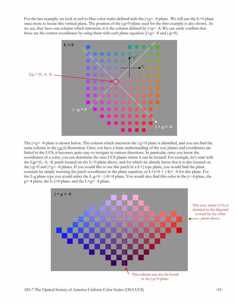
For the last example, we look at red-to-blue color scales defined with the j+g= -8 plane. We will use the L=0 plane once more to locate this vertical plane. The position of the j-g=0 plane used for the first example is also shown. As we see, they have one column which intersects; it is the column defined by j=g= -4. We can easily confirm that these are the correct coordinates by using them with each plane equation (j+g= -8 and j-g=0).

The j+g= -8 plane is shown below. The column which intersects the j-g=0 plane is identified, and you can find the same column in the j-g=0 illustration. Once you have a basic understanding of the way planes and coordinates are linked in the UCS, it becomes quite easy to navigate in various directions. In particular, once you know the coordinates of a color, you can determine the nine UCS planes where it can be located. For example, let’s start with the Ljg=(0, -4, -4) patch located on the L=0 plane above, and for which we already know that it is also located on the j-g=0 and j+g= -8 planes. If you would like to see this patch in a L+j type plane, you would find the plane constant by simply inserting the patch coordinates in the plane equation, or L+j=0 + (-4)= -4 for this plane. For the L-g plane type you would select the L-g=0 - (-4)=4 plane. You would also find this color in the j=-4 plane, the g=-4 plane, the L-j=4 plane, and the L+g= -4 plane.

L = 0

j + g = -8

j - g = 0

j + g = -8

+ g

Ljg = (0, -4, -4)

+j

This column can also be found in the j-g=0 plane.

This row, where L=0, is identical to the diagonal

crossed by the white arrow above.


5. A comparison: A UCS color ramp vs a CIE 1931 color ramp At this point you should be convinced that the UCS space is one of the most, if not the most, uniform color space available! Still, we have not shown one comparison between a color scale derived from it and a more traditional color space. This is what we will present in this section. We will start by isolating a particular scale. We have selected the column located at the intersection of the j-g=0 and j+g= -8 planes discussed in the last example on the previous page. It is shown on the right. The column coordinates are j=g= -4 and L varies from +4 to -8. This column can be found in the following vertical planes: j+g= -8, j-g=0, j= -4, and g= -4. We would not find this column in the other five planes since we are looking for the entire column, and not only a single color. A mini-tutorial is presented below if you want to generate this column with PatchTool. We have selected this scale because it shows a light to dark ramp for a single hue. In the CIE 1931 chromaticity diagram, a single hue is represented by a unique set of x and y coordinates, which remains the same for all luminance or Lightness levels (the Y of xyY or the L* of L*a*b*). We can then easily compare the ramps of the two systems. We first need a reference point in both systems, where the two colors should perfectly match. The chosen reference is the patch with L=0 in the UCS space, which corresponds to L*=58,5 in the CIE system, about midway in the luminance scale. By selecting a midpoint reference, we can better assess how the systems compare above and below the reference point, and without benefiting one system over the other.

Mini-tutorial: How to generate a single color scale with PatchTool The following procedure can be used to generate the single column color scale presented in this section. We want to see the patches where L varies between +4 and -8 for j=g= -4. We will generate the list in such a way that we have a gray border around and between the patches.

1- Open the UCS Tool dialog with the “Tools/OSA UCS…” menu. 2- In ‘Grid options”, click on the “Default” button. Check the “Restrict patches to the following plane” checkbox;

select the UCS “j + g” plane and set the plane value to -8 (minus 8). 3- Select a “List pitch” of 1. Click on the “Reset” button to maximize the range. 4- First adjust L MAX to 5, and then L MIN to -9; these limits are one step higher and lower than the required range

but we will use the extra range as gray background. 5- First adjust j MAX to -3, and then j MIN to -5. As with L, we selected more range than required to generate patches

around our color scale. You will notice that g MIN also changes when j MAX is set, and that g MAX is changed when j MIN is set; these changes are required in order for the j and g coordinates to meet the selected plane equation and plane constant. For our settings, j MAX + g MIN = j MIN + g MAX = -8. A small drawing at the right of the range selection controls shows a cross under j and g, as a reminder of how the coordinates are linked.

6- Under the range selection controls you should now see that the list will consist of 45 patches. 7- In the “Output options”, check the “List only ’All-Even’ and/or ‘All-Odd’ coordinates” check box and click on the

“Even” radio button. We specifically do not want to see colors in the patches with “odd” coordinates located on the adjacent columns; they will be replaced with gray patches. Select the box to keep discarded patches.

8- Keep “unreal” colors. Note: The “unreal” check is redundant since all list colors are within the human eye gamut, but it is a good habit to select it when generating color lists for which it is important to maintain the visual layout.

9- Click on the “Build list” button, save the file when prompted, and close the UCS Tool. Before opening the file in PatchTool, you may want to open the list in a word processor or spreadsheet to see the information it contains. You will see that over two third of the data consists of patches with the UCS background color Ljg=(0, 0, 0).

10- Open the list you just generated with PatchTool. In the UCS Import dialog, select the 2 degree Observer. You should select the 2 degree Observer if you intend to use the color values in printed images or with an ICC managed program (essentially all printing and graphic design tasks), as we do here.

11- If required, you can export this list as an image. If exporting RGB data, you should first select the RGB space in the opened file “Tabular data” Tab. We have selected sRGB for the example above. Then click on the “Export” button or select the “File / ‘Save / Export…’ ” menu.

12- In the “Image” Tab of the “PatchTool Export” dialog, set the image parameters as per your requirements. We selected an RGB file type with 8-bit; you can verify the RGB space in the file below the file name. Note: The illuminant shown under the file name is irrelevant for RGB data since the prescribed RGB space illuminant will always be used.

L = 0


The UCS ramp, imported using the 2 degree Observer, is on the left side of each illustration below; the CIE ramp is on the right side of each illustration. The identical patch in each ramp is the third from the top. The CIE patches were determined as follow:

- The CIE reference was set to UCS patch Ljg=(0, -4, -4), which corresponds, for Illuminant D65 and the 2 degree Observer, to XYZ=(33.71, 26.46, 46.66), xyY=(0.31558, 0.24767, 26.46), and L*a*b*=(58.47, 32.94, -22.39).

- For all other CIE ramp patches, the x and y coordinates were kept constant and their CIE luminance (Y) was matched to the CIE luminance of the UCS patches (this is also true for the Lightness L*).

We see that the patches in the CIE ramp are more saturated than in the UCS ramp for patches with UCS L>0, and are less saturated than in the UCS ramp for patches with L<0. If we drew the corresponding CIE xy chromaticity of the UCS patches, we would see that they are farther from the illuminant for darker patches and that they get closer as UCS L increases; of course the two ramps match at L=0 because this is the selected reference.

The darkest CIE ramp patch is almost black compared with the UCS patch, and the other darker patches have a muddied look. The darkest UCS patch is somewhat too saturated when not fully surrounded by a gray background, in the right illustration, but looks better with the background, on the left illustration. Overall, the UCS ramp is arguably more uniform than the CIE ramp. This is amazing since its equivalent CIE chromaticities are different for each patch; in the CIE reference frame, this means that we should see different hues for each UCS patch, but we definitely don’t!.

UCS ramp CIE ramp

UCS ramp CIE ramp

L* = 79 L = 4

L* = 68

L* = 59

L* = 49

L* = 37

L* = 25

L* = 13

L = 0

L = 2

L = -4

L = -2

L = -6

L = -8

The files for these two ramps are provided with


menu.


6. UCS usage The stock of the original UCS color set made of 558 samples has long been depleted and is no longer available from the OSA. It was recently estimated that preparing the pigments and mixing the paints with a similar precision would be cost prohibitive. Fortunately, because the space was formally mathematically defined, we can regenerate and view these colors on monitors. Also, with modern ink-jet printers, we can print these patches with excellent accuracy and over a greater gamut than the one used in the original development. The OSA UCS has obvious use in any study related to the perception of uniform colors. However, the complexity of the conversion between UCS Ljg and CIE XYZ and the lack of equivalent values for the 2 degree Observer may have limited such studies. It is hoped that the import, export, conversion, and list generation tools in PatchTool can help foster UCS use. For graphic design and artistic painting applications, the unique color scales that can be found in the UCS space offer new possibilities in color harmony. The possibility of getting CIE L*a*b* values for the 2 degree Observer will facilitate the transfer of UCS color scales data in all ICC based applications. And what can the UCS do specifically for color-management people? Here are two such applications, in the form of mini-tutorials. They are presented on the following pages.

- How to check a MONITOR profile with a UCS list filling its gamut

- How to compare the gamut of two devices with a UCS list


Mini-tutorial: How to check a MONITOR profile with a UCS list filling its gamut We suggest you also read the following application note available form the BabelColor Web site:

AN-4a Using PatchTool for IDEAlliance MONITOR proofing certification

There are a few differences between the above document and this tutorial. The IDEAlliance proofing certification uses predefined color lists which cover the gamut of standard press processes, where the color values correspond to standard printing targets, such as IT8.7/4, and where is only important to check that the color list is within the gamut of the monitor used to proof images that will be sent to press. In this tutorial, we take many steps to generate a custom list which completely fills the monitor gamut with a very uniform sampling. You should note that the same procedure can be used to create color lists for any device which is defined by an ICC profile, such as printers or presses.

You can also generate a color list that fills a device gamut with equally spaced L*a*b*, L*C*h*or XYZ coordinates in the Gamut Tools (Look for the “Device independent spaces” section in the “List gen.” Tab). As in this procedure, the list is constrained by a device profile. Such lists are less uniform than UCS lists, but they can be generated much faster.

Please note that some steps of this tutorial require the use of a spreadsheet application.

1- Open the UCS Tool dialog with the “Tools/OSA UCS…” menu. 2- In ‘Grid options”, click on the “Default” button. The “Restrict patches to the following plane” checkbox should

remain unselected. 3- Select a “List pitch” of 2. Click on the “Reset” button to maximize the range. 4- In the “Output options”, the “List only ’All-Even’ and/or ‘All-Odd’ coordinates” check box should be disabled.

Now uncheck the “Keep ‘unreal’ colors (replace by gray)”. These output options will generate colored patches covering the entire plane and will discard unreal colors which are outside of the visible gamut. The maximum number of patches is shown under the range selector. Do not be too concerned by the large number of patches at this point because there are many unreal colors and most of the remaining colors are outside of the profile gamut.

5- Click on the “Build list” button, save the file when prompted, and close the UCS Tool. 6- Open the list you just generated with PatchTool. In the UCS Import dialog, select the 2 degree Observer since we

intend to use to process the list via an ICC profile which is designed to work only with 2 degree Observer data.

7- Change the illuminant from D65, the prescribed UCS illuminant, to D50, the default ICC illuminant. This change is only important if you do a Clip check with Absolute Colorimetric intent in Step-10. Note: The illuminant can remain D65 for the other rendering intents; for these other intents, the data is always converted from the current file illuminant, D65 or another, to D50.

8- Open the Gamut Tools from the Tools menu. Select the “Convert / Clip check” Tab. If not already selected, select the color list you just generated in the PatchTool file menu.

9- In the Destination profile menu, select your monitor profile. If your profile is not present, either browse or drag and drop your profile on this menu control.

10- Select the rendering intent and “Black Point Compensation” setting you plan to use when checking your monitor (Step-21). Typical selections are “Absolute Colorimetric” or “Relative Colorimetric” with BPC.

11- Click on the “Clip check” button located under the “XYZ sent to PCS” label, on the top-right of the dialog. The Gamut Tools will close and a Compare file will be shown.

12- In the Compare file, click in the “More info” checkbox if not selected. Select “Delta E*” and the CIEDE2000 dE formula. Set the left threshold to “>1,0” and the right threshold to “>3,0”. Click once in both threshold border selectors so that thick borders are shown. This section of the Compare window should look as follow: Most of the patches in the Compare file should have red borders (or the color selected for the high threshold if you changed it) and very few patches should have yellow borders. The patches with no borders all returned from the clip check with errors smaller than the lowest threshold. They are usually grouped in clusters, as we see on the next page.

http://www.babelcolor.com/download/AN-4a Using PatchTool for IDEAlliance MONITOR proofing certification.pdf�


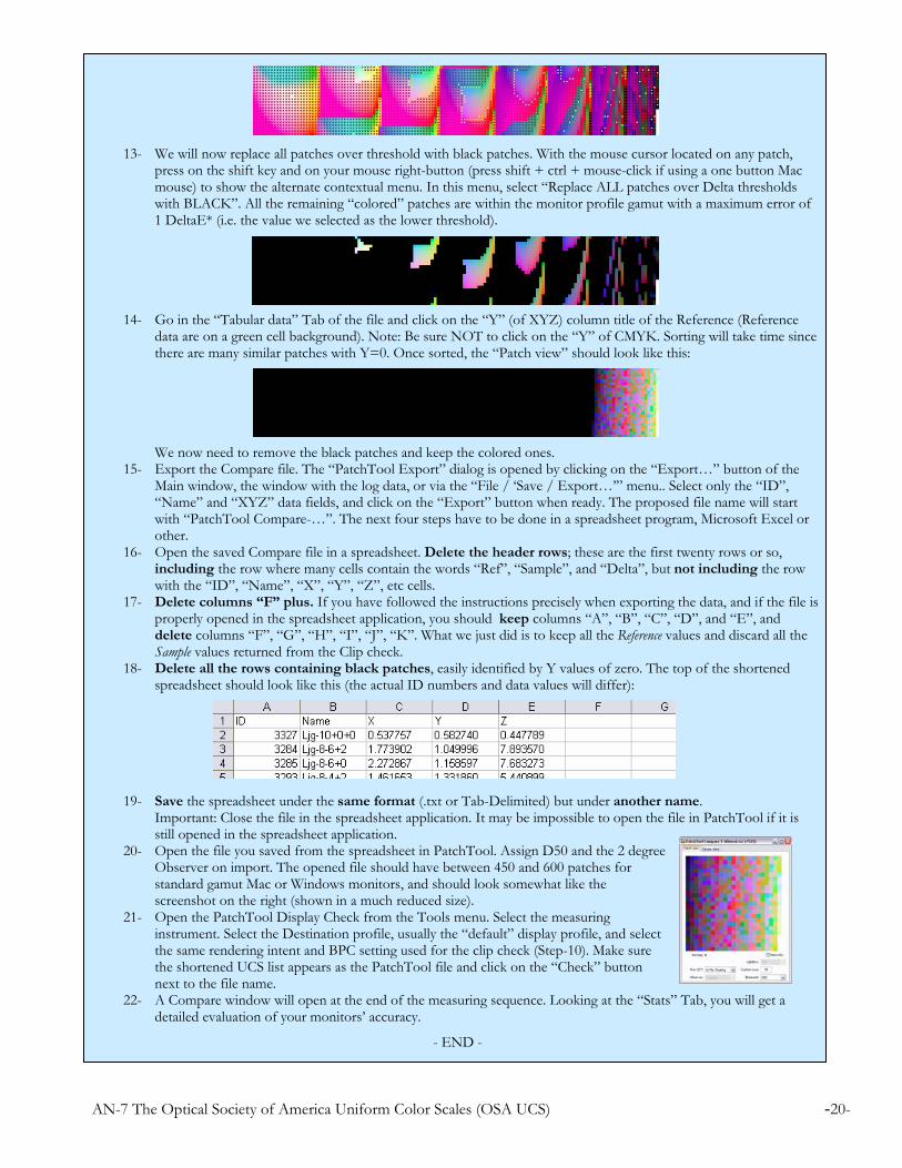
13- We will now replace all patches over threshold with black patches. With the mouse cursor located on any patch, press on the shift key and on your mouse right-button (press shift + ctrl + mouse-click if using a one button Mac mouse) to show the alternate contextual menu. In this menu, select “Replace ALL patches over Delta thresholds with BLACK”. All the remaining “colored” patches are within the monitor profile gamut with a maximum error of 1 DeltaE* (i.e. the value we selected as the lower threshold).

14- Go in the “Tabular data” Tab of the file and click on the “Y” (of XYZ) column title of the Reference (Reference data are on a green cell background). Note: Be sure NOT to click on the “Y” of CMYK. Sorting will take time since there are many similar patches with Y=0. Once sorted, the “Patch view” should look like this: We now need to remove the black patches and keep the colored ones.

15- Export the Compare file. The “PatchTool Export” dialog is opened by clicking on the “Export…” button of the Main window, the window with the log data, or via the “File / ‘Save / Export…’” menu.. Select only the “ID”, “Name” and “XYZ” data fields, and click on the “Export” button when ready. The proposed file name will start with “PatchTool Compare-…”. The next four steps have to be done in a spreadsheet program, Microsoft Excel or other.

16- Open the saved Compare file in a spreadsheet. Delete the header rows; these are the first twenty rows or so, including the row where many cells contain the words “Ref”, “Sample”, and “Delta”, but not including the row with the “ID”, “Name”, “X”, “Y”, “Z”, etc cells.

17- Delete columns “F” plus. If you have followed the instructions precisely when exporting the data, and if the file is properly opened in the spreadsheet application, you should keep columns “A”, “B”, “C”, “D”, and “E”, and delete columns “F”, “G”, “H”, “I”, “J”, “K”. What we just did is to keep all the Reference values and discard all the Sample values returned from the Clip check.

18- Delete all the rows containing black patches, easily identified by Y values of zero. The top of the shortened spreadsheet should look like this (the actual ID numbers and data values will differ):

19- Save the spreadsheet under the same format (.txt or Tab-Delimited) but under another name. Important: Close the file in the spreadsheet application. It may be impossible to open the file in PatchTool if it is still opened in the spreadsheet application.

20- Open the file you saved from the spreadsheet in PatchTool. Assign D50 and the 2 degree Observer on import. The opened file should have between 450 and 600 patches for standard gamut Mac or Windows monitors, and should look somewhat like the screenshot on the right (shown in a much reduced size).

21- Open the PatchTool Display Check from the Tools menu. Select the measuring instrument. Select the Destination profile, usually the “default” display profile, and select the same rendering intent and BPC setting used for the clip check (Step-10). Make sure the shortened UCS list appears as the PatchTool file and click on the “Check” button next to the file name.

22- A Compare window will open at the end of the measuring sequence. Looking at the “Stats” Tab, you will get a detailed evaluation of your monitors’ accuracy.

- END -


Mini-tutorial: How to compare the gamut of two devices with a UCS list Here we give a procedure that can be used to rapidly visually compare the gamut of two devices. By “visually” we do not mean comparing only the “envelope”, or the edge of the gamut, but also the colors that are affected. For the purpose of the example, we compare the sRGB and Adobe RGB color spaces in the UCS L=2,5 plane, which contains a wide range of bright color. We could have compared these profiles with any other UCS plane, with the L= -4 plane for instance, if we were interested in darker shades, or the j+g= -8 plane for a detailed look at the red-blue range. As well, we could also have compared two printer profiles instead, to see which one is better suited to print specific color ranges.

1- Open the UCS Tool dialog with the “Tools/OSA UCS…” menu. 2- In ‘Grid options”, select “Grid steps” of 0,5. Check the “Restrict patches to the following plane” checkbox; select

the UCS “L” plane and set the plane value to +2,5 (plus 2,5). 3- Select a “List pitch” of 0,5. Click on the “Reset” button to maximize the range. This will generate a list with more

than 8000 patches. We could restrict the j and g ranges to lower the number of patches, but we will leave it as is since we do know before hand how large the device gamut will be.

4- In the “Output options”, the “List only ’All-Even’ and/or ‘All-Odd’ coordinates” check box should be disabled. Now check the “Keep ‘unreal’ colors (replace by gray)”. These output options will generate colored patches covering the entire plane and will keep unreal colors which are outside of the visible gamut. This will enable us to better judge how the device gamut covers the human eye gamut.

5- Click on the “Build list” button, save the file when prompted, and close the UCS Tool. 6- Open the list you just generated with PatchTool. In the UCS Import dialog, select the 2 degree Observer since we

intend to use to process the list via an ICC profile which is designed to work only with 2 degree Observer data. 7- Open the Gamut Tools from the Tools menu. Select the “Convert / Clip check” Tab. If not already selected, select

the color list you just generated in the PatchTool file menu. 8- In the Destination profile menu, select the built-in “sRGB (PatchTool)” profile. Select the “Relative Colorimetric”

rendering intent with no BPC. You should not be concerned with the red warning message, below the file name, which indicates that XYZ D65 data will be converted to D50 if the rendering intent is not Absolute Colorimetric, since this is exactly what we want.

9- Click on the “Clip check” button located under the “XYZ sent to PCS” label, on the top-right of the dialog. The Gamut Tools will close and a Compare file will open.

10- In the Compare file, click in the “More info” checkbox if not selected. Select “Delta E*” and the CIEDE2000 dE formula. Set the left threshold to “>1,0” and the right threshold to “>3,0”. Click once in both threshold border selectors so that thick borders are shown. Please look at Step-12 of the previous tutorial to confirm how the interface needs to be set. The Compare window should look as shown on the right. The gray patches on the right side represent “unreal” colors, colors which are outside of the human visual gamut. Most patches have a red border, indicating that these patches are outside of the sRGB gamut by 3 DeltaE* or more. The patches with a yellow border are out of the sRGB gamut by a DeltaE* varying between 1 and 3. All patches with no border are within the gamut or just outside by less than 1 DeltaE*.

11- Redo Steps-7 to 10. You may need to reselect the UCS color list in the Gamut Tools dialog. When redoing Step-8, select the “Adobe RGB (PatchTool)” instead of the previously selected sRGB profile. Click on the “Clip check” button to obtain a second Compare file.

12- The new Compare file should be configured like we did in Step-10, and look as shown on the bottom-right. The difference in gamut can be directly assessed by comparing the relative area covered by each space because the UCS is scaled more uniformly; such a comparison would produce a significant error with most other color spaces, including L*a*b*. If you have a large gamut display, you will also be able to see the extra colors of the Adobe RGB space (all patches are visible on a lower gamut monitor but they are saturated and/or presented with a large error).

13- We can keep only the in-gamut patches and discard the other ones, as we have done in most of the illustrations of this document. With the mouse cursor located on any patch, press on the shift key and on your mouse right-button (press shift + ctrl + mouse-click if using a one button Mac mouse) to show the alternate contextual menu. In this menu, select “Replace ALL patches over Delta thresholds with the 50% GRAY”. All the remaining “colored” patches are within the selected gamut with a maximum error of 1 DeltaE*. The “cleaned’ versions of these images are shown on the next page.


This zone is outside of the human visual gamut

(‘unreal’ colors).

While the larger gamut of Adobe RGB is “real”, the extra colors can only be

appreciated on a wide-gamut monitor!

sRGB gamut for UCS L = 2,5

Adobe RGB gamut for UCS L = 2,5


7. Conclusion This document’s goal was to familiarize the reader with the Optical Society of America Uniform Color Scales (OSA UCS). We hope that we have shown enough of its features to entice the reader to look at it further, and maybe even use it! Like with all other color spaces, one needs to spend some time using the UCS before feeling at ease with it. The UCS unusual geometry may rebuff many at first sight, but it becomes surprisingly straightforward to navigate within its planes and color-scales directions after a few trials. This said, a 100% percent understanding of its idiosyncrasies is not required to take advantage of what it offers, and one could well generate, use, and appreciate its color scales without a perfect grasp of the mathematics behind it. When looking at the images of the tutorial on the preceding page, one is reminded of a geographic map with uncharted territories. This is a quite analogous to where the UCS stands in the color world. Many studies were performed during its conception, but the exceptionally long time it took to finalize its specifications had a toll on the patience of its creators as well on how it was perceived by others. Some may argue that it is useless to spend time on the UCS when it is now acknowledged that a color system based on only three parameters cannot describe uniformly all the colors humans can perceive. Yet, there are recent publications which continue the analysis of this space, and others which use it as uniform color space reference. And we could add that we do spend a lot of time everyday with color spaces which are much worse! As a minimum, the UCS can provide a different perspective on color, which, while not new because it has been with us in its final form for over thirty years, is still mostly unknown.

September 20, 2009 I would like to thank Mrs. Joy Turner Luke who recently presented me a meticulously assembled binder containing an index of the UCS in the form of thousands of small tiles ordered as per the geometry of the standard UCS planes. We are talking here of many thousands of tiles, because a given UCS color can be found in up to 9 planes, and thus nine pages of the index! Joy has spent a large part of her life promoting color to all who would benefit from a greater knowledge of it. She is the co-author of a best-selling book on the applications of the Munsell Color System; she has long been involved with numerous professional societies devoted to color and still participates in international standards committees. She worked with, and knew personally, many of the UCS committee members, and it is thus not a surprise to see her promote the UCS. When I first saw these color scales, I immediately notice their originality, a first impression which is maintained after many hours of observation. The discussions we had thereafter incited me to support the UCS space and add dedicated tools for it in PatchTool. For those interested in the history of the UCS, you will find fascinating that the tiny patches used in the indexes assembled by Joy were saved from oblivion by someone who carefully recuperated and classified the clippings of the 558 tiles of the 1977 UCS proof-of-concept. These clippings, of irregular shapes and sizes, were smaller than the original 2 in by 2 in (50 mm x 50 mm) tile size required for the issue, and thus rejected; they were given to Joy by Jarus Quinn, OSA’s first Executive Director. By cutting the clippings down to about 0,250 to 0,375 inch (6 to 10 mm), there are now enough mini-tiles to generate a few dozens indexes. If you have an interest in acquiring an index made from the original UCS samples, please send me an email and I will forward it to her.

Danny Pascale

[email protected]

mailto:[email protected]?subject=Interest%20in%20UCS%20Index�


“BabelColor” is a registered trademark, and the BabelColor logos and “PatchTool” are trademarks of Danny Pascale and The BabelColor Company.

“IDEAlliance” is a registered trademark of International Digital Enterprise Alliance, Inc. All other product and company names may be trademarks of their respective owners.

© 2009 Danny Pascale and The BabelColor Company

The BabelColor Company

Founded in 2003, The BabelColor Company is dedicated to the development and sale of

specialized color translation software and color tools. It also provides color consulting services for

the professional and industrial markets.

[email protected]

http://www.BabelColor.com

mailto:[email protected]?subject=Info%20required�

http://www.babelcolor.com/�

an-7 the optical society of america uniform color … the osa ucs.pdf · the optical society of...

Documents