amesim and titre‘common rail type injection systems · amesim and ‘common rail’ type...

Technical Bulletin n°110

Titre AMESim and ‘Common Rail’ type Injection Systems

www.amesim.com – www.amesim.com - www.amesim.com

Copyright IMAGINE S.A. 1995-2002

How to contact IMAGINE: North America [email protected] Europe [email protected] Asia [email protected] Visit www.amesim.com for further contact information and details on other countries. Copyright IMAGINE S.A. 1995-2002 AMESim® and AMESet® are the registered trademark of IMAGINE SA. All other product names are trademarks or registered trademarks of their respective companies Latest update: Feb. 26th, 2002

AMESim and Common Rail type injection systems 3/17



AMESim and ‘Common Rail’ type Injection Systems

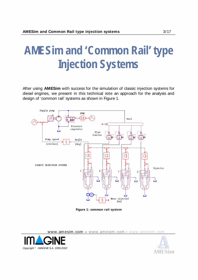
After using AMESim with success for the simulation of classic injection systems for diesel engines, we present in this technical note an approach for the analysis and design of ‘common rail’ systems as shown in Figure 1.

Figure 1: common rail system




This approach is illustrated using an injection system for a diesel engine (with pressure in excess of 1 000 bar). The same approach has been used with success for gasoline engine injection systems (with a pressure of several tens of bar), the structure of which is almost identical to that of the diesel injection systems.

1. Introduction Simulation plays a central role in the analysis and conception of these complex systems. It helps significantly in answering different questions concerning the behavior of components such as pumps, injectors, flow limiters, pressure regulators. It also helps in the sizing of the injection circuit as a whole. The answers to the different questions are not direct, and thus, it is not sufficient to create a complex model of the entire system to elucidate the behavior. It is by the exploitation of well-chosen models of varying complexity that we arrive at an understanding and thus the mastering of the system.

2. Components modeling

We shall present the models of the different components which make up the injection system: the pump, the pressure limiter, the flow limiter, the injector and the fluid circuit. The descriptions presented are not exhaustive in terms of modeling hypotheses and analysis of results since this is not the aim of this technical bulletin. We limit ourselves to the illustration of the applicability of AMESim to this type of problem.

2.1 High pressure pump

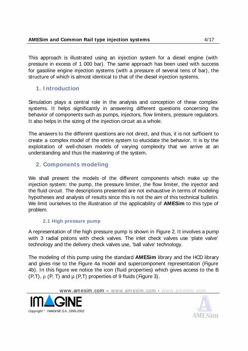
A representation of the high pressure pump is shown in Figure 2. It involves a pump with 3 radial pistons with check valves. The inlet check valves use ‘plate valve’ technology and the delivery check valves use, ‘ball valve’ technology. The modeling of this pump using the standard AMESim library and the HCD library and gives rise to the Figure 4a model and supercomponent representation (Figure 4b). In this figure we notice the icon (fluid properties) which gives access to the B (P,T), ρ (P, T) and µ (P,T) properties of 9 fluids (Figure 3).




Figure 2: 3 piston pump (doc. REXROTH)

Figure 3: different fluids




Figure 4a: pump model Figure 4b : supercomponent

representation The model is tested by connecting it to an orifice adjusted to give 1 000 bar at the pump outlet. The exploitation of this model can give rise to different analyses:




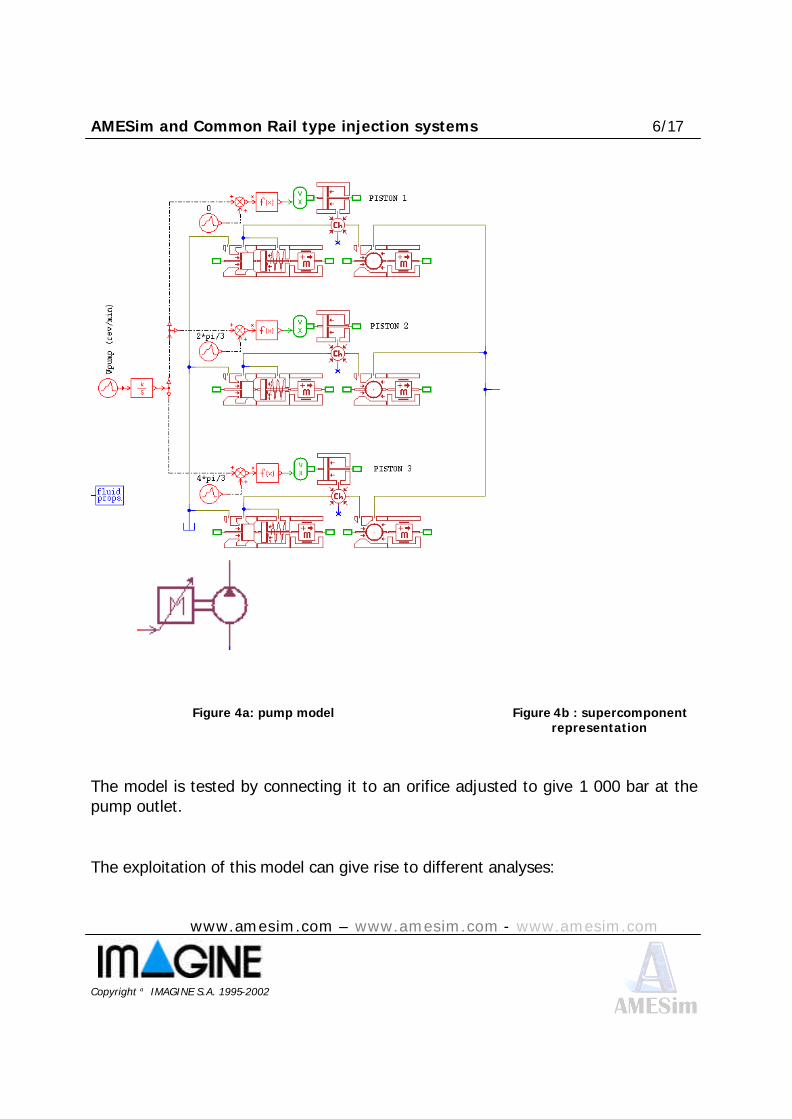
• We determine the average flow rate in the orifice, • We determine the evolution of the pressure into the volume as shown in

Figure 5, • Figure 6 shows a result of a F.F.T. (Fast Fourier Transformation) applied

to the pressure signal. This spectrum is interesting because, theoretically, the kinematics of the pump has a first frequency pressure signal at:

f = 2Nω [Hz]

where : N = number of pistons ω = rotary speed The F.F.T. shows a first frequency at Nω. This phenomenon is due to the compressibility effect in each cylinder.

Figure 5: pressure at the pump outlet

Figure 6: Fast Fourier Transform (FFT) of the

output pressure




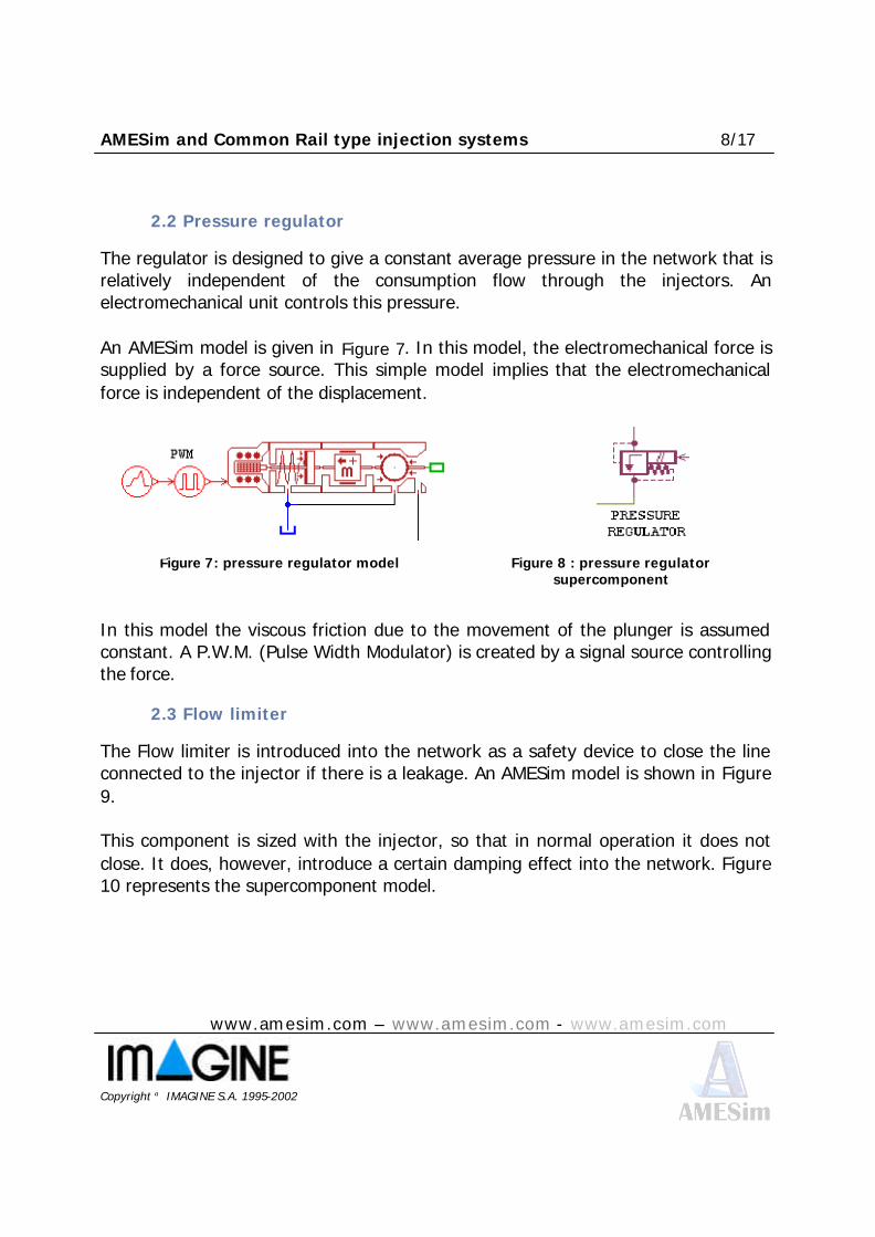
2.2 Pressure regulator

The regulator is designed to give a constant average pressure in the network that is relatively independent of the consumption flow through the injectors. An electromechanical unit controls this pressure. An AMESim model is given in Figure 7. In this model, the electromechanical force is supplied by a force source. This simple model implies that the electromechanical force is independent of the displacement.

Figure 7: pressure regulator model Figure 8 : pressure regulator supercomponent

In this model the viscous friction due to the movement of the plunger is assumed constant. A P.W.M. (Pulse Width Modulator) is created by a signal source controlling the force.

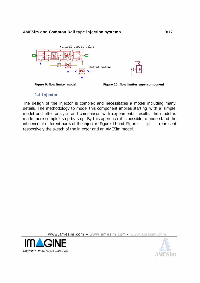
2.3 Flow limiter

The Flow limiter is introduced into the network as a safety device to close the line connected to the injector if there is a leakage. An AMESim model is shown in Figure 9. This component is sized with the injector, so that in normal operation it does not close. It does, however, introduce a certain damping effect into the network. Figure 10 represents the supercomponent model.




Figure 9: flow limiter model Figure 10: flow limiter supercomponent

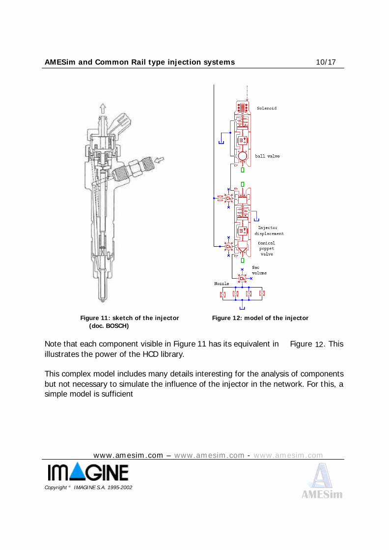
2.4 Injector

The design of the injector is complex and necessitates a model including many details. The methodology to model this component implies starting with a ‘simple’ model and after analysis and comparison with experimental results, the model is made more complex step by step. By this approach, it is possible to understand the influence of different parts of the injector. Figure 11 and Figure 12 represent respectively the sketch of the injector and an AMESim model.




Figure 11: sketch of the injector Figure 12: model of the injector

(doc. BOSCH) Note that each component visible in Figure 11 has its equivalent in Figure 12. This illustrates the power of the HCD library. This complex model includes many details interesting for the analysis of components but not necessary to simulate the influence of the injector in the network. For this, a simple model is sufficient




2.5 Hydraulic network

The analysis of the dynamic behavior of a hydraulic line is relatively complex. The behavior of a line can be dominated by:

• Compressibility effect, • Compressibility and dissipative effects, • Wave effect where the inertia compressibility and dissipative effects are

significantly coupled. It is easy to provide some general dynamic characteristics of a line related to simple boundary conditions (line ‘close-close’, ‘close-open’, ‘open-open’). From this behavior it is possible, with some expertise, to estimate the behavior of a line with more general boundary conditions. For a hydraulic network, the problem is much more complex. The interaction between different lines of different characteristics: length, diameter, stiffness, induce a behavior which is more difficult to analyze. Moreover, due to the interaction between different lines, the choice of the line models is not easy. If we take a complex line model at each part of the circuit, the size of the state equation will be enormous. The simulation time will be unacceptable. If the model is too simple the results will be poor. From these considerations it appears that time domain simulations are not well adapted to analyze the network and choose the best models. A better alternative is a linear analysis approach.

2.5.1 Basic discussion

We have a non-linear model with the classical form:

( )( )

& ,

,

x f x u

y g x u

=

=

or

( )( )

0 =

=

f x x u

y g x u

&, ,

,




We are able to calculate with AMESim the linear tangent solution. This is the linear form of the state equation:

&x Ax Bu

y Cx Du

∗ ∗ ∗

∗ ∗ ∗

= +

= +

This linear state equation is available at the equilibrium point ( &x = constant with u = constant).

2.5.2 Why use linear analysis?

Linear analysis permits the analysis of the intrinsic properties of the system, independent of the inputs. The linear model is simpler to analyze than a non-linear model. The frequency domain is easy to calculate from a linear model:

• Transfer function • Modal analysis

The linear analysis helps in choosing the type of line model of the different parts of the network. The calculation of the time response of the non-linear model can be minimized by this approach. It is particularly useful when the excitation of the circuit is periodic (the most common case), e.g.:

• Ripple of the flow rate from the pump • Pressure regulator controlled by the P.W.M. • Opening and closing of the injectors at a certain frequency.




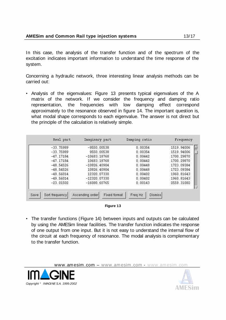
In this case, the analysis of the transfer function and of the spectrum of the excitation indicates important information to understand the time response of the system. Concerning a hydraulic network, three interesting linear analysis methods can be carried out: • Analysis of the eigenvalues: Figure 13 presents typical eigenvalues of the A

matrix of the network. If we consider the frequency and damping ratio representation, the frequencies with low damping effect correspond approximately to the resonance observed in figure 14. The important question is, what modal shape corresponds to each eigenvalue. The answer is not direct but the principle of the calculation is relatively simple.

Figure 13

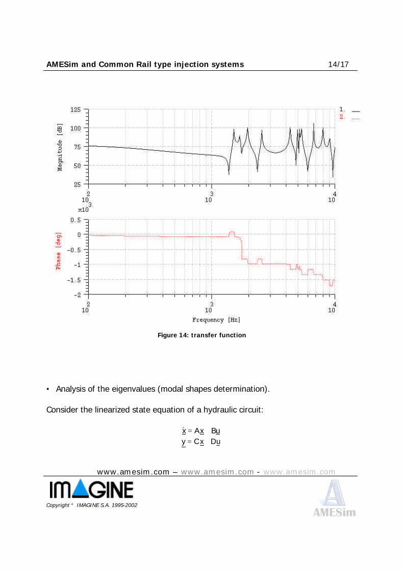
• The transfer functions (Figure 14) between inputs and outputs can be calculated

by using the AMESim linear facilities. The transfer function indicates the response of one output from one input. But it is not easy to understand the internal flow of the circuit at each frequency of resonance. The modal analysis is complementary to the transfer function.




Figure 14: transfer function

• Analysis of the eigenvalues (modal shapes determination). Consider the linearized state equation of a hydraulic circuit:

&x Ax Bu= + y Cx Du= +




If we consider the T matrix such as TAT 1−=Λ is diagonal, the terms of the diagonal of Λ matrix are the eigenvalues λi and T matrix represent the eigenvectors. Now, we can consider the initial system represented in the modal basis such as:

&z T ATz T Bu= +− −1 1 and the relation with the new variable z and the observer vector y is :

y CTz= The solution of this system is:

( ) ( ) ( ) ( )z t e z e V r driit

ii t rt

i= + −∫λ λ00

If we consider z (0) = 0 and Vi = δ (0) = Dirac function, the solution becomes:

z i (t) = eλit and: ( )tzCTy=

where y is a modal shape. With this result it is interesting to consider two cases: Case 1: λi are real or complex conjugate pairs with a non-zero real part

In this case, the modal shape evolves with time. Case 2: λi are purely imaginary

The system is ‘conservative’ (no dissipation), the mode shape have an oscillation form.

The interpretation of the first case is not easy without animation (except with a simple system). The second case is easy to represent.




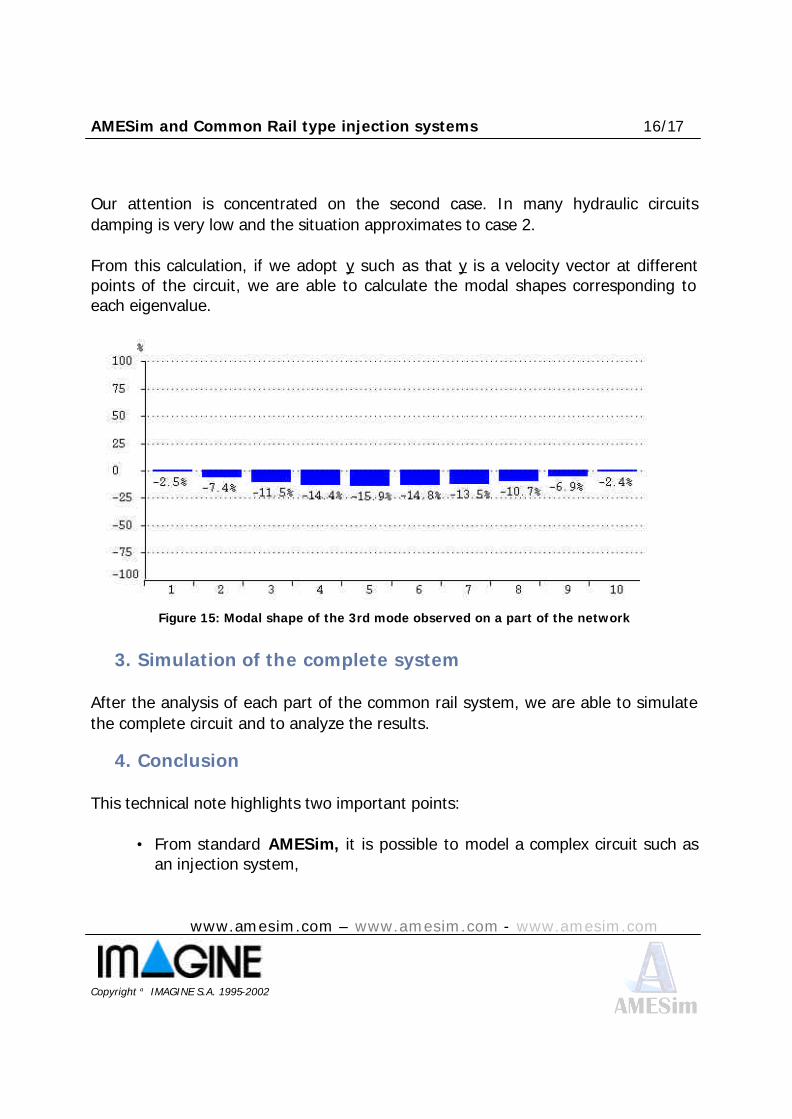
Our attention is concentrated on the second case. In many hydraulic circuits damping is very low and the situation approximates to case 2. From this calculation, if we adopt y such as that y is a velocity vector at different points of the circuit, we are able to calculate the modal shapes corresponding to each eigenvalue.

Figure 15: Modal shape of the 3rd mode observed on a part of the network

3. Simulation of the complete system

After the analysis of each part of the common rail system, we are able to simulate the complete circuit and to analyze the results.

4. Conclusion

This technical note highlights two important points:

• From standard AMESim, it is possible to model a complex circuit such as an injection system,




• The AMESim software is adapted to help the learning process and the

design process. A good methodology can be applied to analyze and understand the studied system.

amesim and titre‘common rail type injection systems · amesim and ‘common rail’ type...

Documents