america’s first great moderation - cambridge.org · the journal of economic history, vol. 77, no....

1116

The Journal of Economic History, Vol. 77, No. 4 (December 2017). © The Economic History Association. All rights reserved. doi: 10.1017/S002205071700081X

Joseph Davis is Global Chief Economist, The Vanguard Group, Valley Forge, PA 19482-2600. E-mail: [email protected]. Marc D. Weidenmier is Professor of Finance, Chapman University, 1 University Drive, Orange, CA 92866. E-mail: [email protected].

We thank Barry Eichengreen, Christina Romer, David Romer, Christopher Hanes, Joseph Ferrie, Lou Cain, and Marcelle Chauvet as well as seminar participants at UC-Berkeley, UC-Riverside, Northwestern University, and the NBER Summer Institute for helpful comments and suggestions. We thank Ryan Shaffer for superb research assistance.

1 Hunt’s Merchant Magazine and Commercial Review, January 1853, p. 73. The opening quote was also preceded by the following statement. “The year now drawing to a close, and which will be reckoned with the past when this reaches the eyes of our readers, has been one of signal commercial prosperity throughout the whole of the American Union. We have formerly had seasons of expansion, when nominal fortunes have been reckoned in a multitude of hands; never before since the rst colony was planted on our shores, has the country made such rapid strides in wealth, upon a substantial basis.”

America’s First Great ModerationJOSEPH DAVIS AND MARC D. WEIDENMIER

We identify the longest expansion in U.S. history, a recession-free 16-year period from 1841 to 1856 that we call America’s First Great Moderation. Using newer data on industrial production, we show that the record-long expansion was primarily driven by a boom in transportation-goods investment following the discovery of gold in California. Furthermore, the low volatility of industrial production and stock returns during the First Great Moderation, which occurred during a period without a U.S. central bank, is similar to that observed for the Second Great Moderation (1984–2007).

“Our merchants have never enjoyed such uninterrupted prosperity.”1

The Great Moderation is a term frequently used to describe a period of low macroeconomic volatility and positive economic growth

observed in the United States from 1984 until the onset of the global nan-cial crisis beginning in 2007 (Stock and Watson 2002). The signi cant reduction in the volatility of real output over this period is also associated with less frequent and less severe U.S. recessions. Indeed, according to the National Bureau of Economic Research’s (NBER) monthly business cycle chronology, three of the four longest U.S. expansions following WWII occurred during the Great Moderation, including the 120-month expansion of the 1990s, commonly viewed as the longest expansion in U.S. history to date.

Economists have offered three types of explanations for the marked decline in macroeconomic volatility between the mid-1980s and the late

http://crossmark.crossref.org/dialog/?doi=10.1017/S002205071700081X&domain=pdf

America’s First Great Moderation 1117

2000s. Some have argued that improved monetary policy is a primary reason for the large drop in macroeconomic volatility (Stock and Watson 2002; Bernanke 2004). Other research has pointed to structural change that has made the economy less sensitive to shocks, including the shift of economic production from goods to services, improved management of inventory investment through information technology, and innovations in nancial markets that promote intertemporal smoothing of consump-tion and investment (Blanchard and Simon 2001; McConnell and Perez-Quiros 2000). Several studies have also pointed to “good luck,” or the absence of large shocks (i.e., oil shocks or technology shocks) as impor-tant factors that help explain this period of unusually low business cycle volatility (Ahmed, Levin, and Wilson 2004). While the sources of the Great Moderation certainly remain open to debate and require further research, the conventional wisdom is that there has been only one Great Moderation in U.S. history.

We break new ground in this article by identifying America’s First Great Moderation. From 1841 to 1856, the United States experienced a 16-year economic expansion that was characterized by high economic growth rates, especially for investment goods such as transportation machinery.2 The U.S. economy escaped downturns during this period in part because economic growth was so high. Trend growth during the 1840s and 1850s in both Robert Gallman’s real GNP series and Joseph Davis’s industrial production index (IP) were the highest of the nine-teenth century (Gallman 1966; Davis 2004). Economic and nancial market volatility were signi cantly lower, too. We consult newer, high-frequency series in our statistical analyses, including annual industrial production (the most reliable indicator of business cycles for this period) and monthly stock prices (as an even higher-frequency indicator of nan-cial conditions and panics).

We test a number of hypotheses that could explain America’s First Great Moderation. Our empirical evidence suggests that the moderation was the result of the wider adoption and diffusion of transportation tech-nologies including clipper and steam ships, locomotives and railroads. Through both Markov-switching models and Granger-causality tests, we show that the Great Moderation would not have occurred without transportation-related activity. In particular, America’s longest economic

2 We consider the First Great Moderation to be the longest expansion in American history because the period did not experience negative economic growth as measured by the Davis IP index between 1841 and 1856. In contrast, the modern Great Moderation period from 1984–2007 did not have an expansion lasting more than nine years using the Hodrick-Prescott lter.

Davis and Weidenmier1118

expansion may well have ended by 1850 had it not been for the discovery of gold in California, which signi cantly increased the expected returns for massive clipper ships that could sail to New York in as little as 100 days and circumnavigate the globe.3 The spillover effects of this transpor-tation boom were meaningful; indeed, the 1841–1856 period was unique in the pre-WWI era for transportation-related output to lead the rest of the industrial sector. Furthermore, we fail to nd compelling evidence that agriculture (i.e., cotton), weather, domestic textile production, immigra-tion, or British economic conditions played an important role in causing America’s First Great Moderation. While we cannot rule out that certain other factors—including western expansion, increased nancial market integration, lower and stable tariffs, and state constitutional reforms—may have played some role during this time, they likely would have had to have worked through the transportation sector and stock prices.

The article begins with a brief history of the pre-Civil War economy of the 1840s and 1850s, especially in the context of early American busi-ness cycles. We then compare the economic and nancial performance of the First Great Moderation with other periods before the outbreak of WWI in 1914. We employ Markov-switching models to assess the decline in macroeconomic and nancial market volatility in the First Great Moderation. Using similar IP and stock-price data, we then conduct an apples-to-apples comparison of our First Great Moderation to the modern-day Great Moderation that ran from the mid-1980s until the onset of the global nancial crisis in 2007. Notably, our Markov-switching models reveal that the low-volatility, high-growth states derived for the First Great Moderation are of similar magnitude and statistical signi cance to those estimated for the contemporary one using compa-rable economic and stock-market data. Finally, we contemplate various factors—both structural and fortunate—that help explain the First Great Moderation.

THE ANTEBELLUM U.S. ECONOMY AND THE FIRST GREAT MODERATION

In the two decades prior to its Civil War, the American economy grew rapidly by nearly any measure in the Historical Statistics of the United States (Carter, Gartner, and Haines et al. 2006, Parts C and D). U.S.

3 Hobsbawm (1975) argues that the California gold rush reinvigorated the global economy by increasing the money supply.


real GNP grew at more than a 5 percent annualized rate between the mid-1840s and late 1850s, versus still-high yet lower rates of growth during the development of the U.S. economy in the late 1800s (Rhode 2002).4 In short, the decades of the 1840s and 1850s witnessed the most robust rates of economic growth of the nineteenth century. Indeed, per capita GNP rose more than 30 percent (Gallman 2000, p. 50). Annual growth in the Davis (2004) industrial production index averaged more than 7.6 percent between 1841 and 1856. We now turn to a discussion of economic factors that might explain the high trend growth rate of the First Great Moderation.

Between 1840 and 1860, the rates of immigration and the size of the U.S. labor force doubled, while the urban population tripled (Carter, Gartner, and Haines et al. 2006, Part A). Federal land sales and westward migration led to signi cant farmland development and growing transpor-tation networks beyond the large eastern coastal cities. The relatively high rate of population growth as well as the in ux of immigration increased aggregate production and should have reduced the probability of a reces-sion. The high rates of economic growth during the 1840s and 1850s were also accompanied by more integrated nancial and labor markets (Bodenhorn 1992, 2000). Increased nancial market integration may help explain the high rates of capital investment during the 1840s and 1850s by reducing business uncertainty and raising con dence (Davis 1966). Real wages converged across the country and became less vola-tile, forming the beginnings of a more ef cient and integrated “national labor market” (Margo 1998, p. 1).5

A fast-growing and more-integrated economy with advancing capital markets would seem to suggest the United States experienced less frequent and less violent downturns during the 1840s and 1850s. Qualitatively, however, the early foundations of today’s of cial NBER business-cycle chronology suggest a volatile economy. According to William L. Thorp’s Business Annals (1926) and Arthur F. Burns and Wesley C. Mitchell’s Measuring Business Cycles (1946)—two seminal NBER studies that laid the groundwork for the of cial monthly NBER business-cycle dates before 1920—the U.S. economy spent nearly half of the years in reces-sion between the late 1830s (following the Panic of 1837) and the onset

4 We rely on Gallman’s (1966) GNP data which is based on the U.S. Census.5 In addition, Vandenbrouke (2008) demonstrates that western/eastern real wage ratios, which

had widely varied prior to the early-to-mid 1840s, declined and remained relatively stable for the remainder of the antebellum period.


of the Civil War.6 The depression of 1839 is believed to have ended in 1843 or perhaps as late as 1845.7 Recessions and panics are noted for 1846, 1848, and 1854. Based more on anecdotal newspaper reports than economic data, the Annals tend to re ect nancial market conditions and price corrections rather than business cycles.8

INDUSTRIAL PRODUCTION DATA

We consult economic and nancial data in our statistical analyses of the early American business cycle, including annual industrial production and monthly stock prices. With access to better data, we nd America’s First Great Moderation. Our primary measure of the business cycle during America’s First Great Moderation is the Davis (2004) quantity-based industrial production (IP) index. The Davis IP index is comprised of 43 annual components in the manufacturing and mining industries that are consistently de ned from 1790 until WWI. It is a comprehensive industrial output measure in so far as its components directly or indirectly represent close to 90 percent of the value added produced by the U.S. industrial sector during the nineteenth century. Changes in the Davis IP index re ect uctuations in real output.

While the Gallman real GNP data are somewhat more comprehensive than the Davis IP index, the annual estimates themselves are far less reli-able. Gallman himself did not trust the accuracy of his annual time series, declining to ever publish them and instead using them to infer trends in ante-bellum growth. As Paul W. Rhode (2002) notes, Gallman wrote, “that these data were not constructed for analysis as annual series,” and wrote: “NOTE: These gures should not be regarded as reliable, annual estimates.”9

Figure 1 charts logarithmic growth rates in the Davis IP index from 1792 through 1914. In the gure we highlight the 1841–1856 period,

6 Hammond (1957) argues that the Second Bank of the United States brought stability to the U.S. economy during the 1820s and early 1830s.

7 Temin (1969), on the other hand, argues that the “recession” from 1839–1843 was a period of de ation rather than a depression.

8 By consulting contemporary newspaper accounts and uctuations in commodity and stock prices, Thorp’s Business Annals summarizes business conditions in 1845 as “prosperity; brief recession,” 1846 as “recession, mild depression,” 1847 as “revival; prosperity; panic; recession,” and 1848 as “mild depression; revival.” Kindleberger (2000), refers to a number of nancial panics during the late 1830s, 1840s, and 1850s that were believed to have led to signi cant recessions, de ation, and, at times, depressions. Recent research by Jalil (2015) questions the accuracy of Thorp’s listing of banking crises.

9 As discussed in Rhode (2002) and Davis (2002), other provisional GNP estimates for the pre-Civil War economy (such as Berry’s series) are inappropriate to date business cycles (Berry 1978; Carter, Gartner, and Haines et al. 2006, Parts C and D). By contrast, the Davis index incorporates new source data across a host of sectors that had direct ties to the agricultural and export markets of the early U.S. economy.


which we will call America’s First Great Moderation. Table 1 compares the average growth rate in real output (as de ned by the annual Davis IP index) during the First Great Moderation (1841–1856) with the sample periods before and after its occurrence. Based on the annual Davis IP series, we nd that industrial production growth averaged nearly 8 percent per annum during the First Great Moderation, compared to an average growth rate of approximately 5 percent for the rest of the 1792–1914 period. Overall, the growth rate of IP was 60 percent higher on average during the First Great Moderation than in either of the preceding or subsequent sample periods. This acceleration in industrial growth paral-lels and corroborates the acceleration in growth of Gallman’s real GNP series.10

During the antebellum period, the differences in average growth rates between the Great Moderation and other years are statistically signi cant (p=0.04), compared to insigni cant differentials between the antebellum and post-bellum periods (see bottom of Table 1). One would expect average IP growth to be higher during the First Great Moderation since there were no absolute annual declines in industrial production between 1841 and 1856. The high rate of growth in industrial production was

-.20

-.15

-.10

-.05

.00

.05

.10

.15

.20

-.20

-.15

-.10

-.05

.00

.05

.10

.15

.20

1800 1810 1820 1830 1840 1850 1860 1870 1880 1890 1900 1910

Inde

x lo

garit

hmic

gro

wth

rate

s

FIGURE 1GROWTH RATES IN ANNUAL DAVIS IP INDEX, 1792–1914

Notes: Gray areas represent declines in the Davis IP index, which we associate here with recessions, as in Davis (2006). The shaded area represents the First Great Moderation.Sources: Davis (2002, 2004, 2006); authors’ calculations.

10 Other periods of expansion in Davis’s annual IP index from 1792–1915 covering a minimum of ve years include (in descending order): 1865–1873, 1875–1883, 1885–1892, 1896–1903, and 1823–1828.


accompanied by low volatility. The standard deviation of IP growth was 5 percent between 1841 and 1856. For the antebellum period before the start of the First Great Moderation, the standard deviation of industrial production growth averaged 6.7 percent. The standard deviation of IP growth averaged 7.5 percent in the post-bellum period. As is the case with mean growth rates, volatility differences in IP growth between the Great Moderation and the antebellum years between 1792–1840 are statistically signi cant (p=0.098), compared to insigni cant differentials between the antebellum and post-bellum eras (p=0.355). We also employ the coef cient of variation (standard deviation divided by the mean) to control for the fact that the average growth rate in IP was higher during the First Great Moderation. Table 1 shows that the coef cient of variation for industrial production during the First Great Moderation, at 0.65, was notably lower when compared to 1.45 for the antebellum period and 1.63 for the post-bellum period. The basic summary statistics indicate that industrial production growth was higher and IP volatility signi cantly lower during the First Great Moderation.

We corroborate our annual IP-based results using a monthly series on stock prices, which should afford an even higher-frequency indicator of nancial conditions and “panics” sometimes cited in the qualitative

TABLE 1SUMMARY STATISTICS FOR U.S. INDUSTRIAL PRODUCTION GROWTH, 1792–1914

Davis IP Index, Log Growth Rates

Period Dates

Mean Growth

(Percent)Standard Deviation

Coef cient of Variation

Full sample 1792–1914 4.86 0.069 1.41Antebellum, pre-Great Moderation 1792–1840 4.65 0.067 1.45Great Moderation 1841–1856 7.66 0.050 0.65Postbellum, pre-WWI 1867–1914 4.61 0.075 1.63

Memo: Statistical equivalence tests of mean and standard deviation

Period

GM vs. non-GM antebellum 0.04** 0.098*Across all 3 sub-samples 0.12 0.193Antebellum vs. postbellum 0.65 0.355

* = Signi cant at the 10 percent level.** = Signi cant at the 5 percent level. *** = Signi cant at the 1 percent level.Sources: Davis (2004); authors’ calculations.

Satterthwaite-Welch Mean Equality t-test, p-value

Equality of Variance F-test, p-value


characterizations of the contemporary economy. Speci cally, we employ William N. Goetzmann, Roger G. Ibbotson, and Liang Peng’s (2005, hereafter GIP) pre-CRSP era stock index from 1815–1914 to examine stock returns and stock volatility during the First Great Moderation. The GIP pre-CRSP era NYSE series is among the most comprehensive monthly stock market series for the nineteenth century. While other city-level stock price series exist for the antebellum period (Schwert 1990), we focus on the GIP series since it spans the entire nineteenth century and tends to include more securities than other stock indices, such as Smith and Cole’s price index (Smith and Cole 1935).

Table 2 shows that stock returns averaged 0.3 percent per month during the Great Moderation. Average stock returns for the GIP Index were negative in the antebellum period before the Great Moderation, and aver-aged 0.17 percent per month in the post-bellum period. Stock volatility, as measured by the standard deviation of monthly price returns, averaged 3.5 percent during the First Great Moderation, compared to 3.9 percent and 4 percent in the antebellum and post-bellum periods, respectively. The lower stock-market volatility for the Great Moderation is statisti-cally signi cant and is more than 20 percent lower than the non-Great Moderation antebellum period and more than 10 percent lower than the

U.S. Stock Prices, Monthly Price Returns

Period Dates

Mean Growth

(Percent)Standard Deviation


Full sample 1826M1–1914M12 0.19 0.040 21.21

Antebellum, pre-Great Moderation 1826M1–1840M12 –0.15 0.039 (25.78)

Great Moderation 1841M1–1856M12 0.30 0.035 11.44

Postbellum, pre-WWI 1868M1–1914M12 0.17 0.040 23.35

Memo: Statistical equivalence tests of mean and standard deviation

Period

GM vs. non-GM antebellum 0.19 0.008***Across all 3 sub-samples 0.47 0.052*Antebellum vs. postbellum 0.60 0.651

TABLE 2SUMMARY STATISTICS FOR EARLY U.S. STOCK RETURNS, 1826–1914

Satterthwaite-Welch Mean Equality t-test, p-value

Equality of Variance F-test, p-value

* = Signi cant at the 10 percent level.** = Signi cant at the 5 percent level. *** = Signi cant at the 1 percent level.Sources: Goetzmann et al. (2001); authors’ calculations.


post-bellum period. The coef cient of variation for stock returns during the First Great Moderation, 11.44, is approximately one-half that of the coef cient of variation for either the earlier antebellum period (25.78) or post-bellum period (23.35). Overall, we nd that stock returns were both higher and signi cantly less volatile than the rest of the pre-WWI period.

IDENTIFYING BUSINESS CYCLES

Focusing on industrial production rather than broad GDP or even nonagricultural GDP could be a potential limitation of our study if (and only if) IP was not re ective of the broader economy during this era. We argue that this was not the case, for several reasons. As discussed in Davis (2004), IP is appropriate to de ne the historical evolution of U.S. business cycles, if for no other reason than the fact that America’s emergence as an economic power is commonly equated with its industri-alization. While more than one-half of national output in the antebellum United States was agricultural, the Davis IP index should be broadly indicative of the nation’s economic conditions because the industrial sector has historically derived demand directly from nonindustrial occu-pations, particularly farmers, merchants, and the construction trades.11 The processing of foodstuffs, the demand for agricultural machinery, and the capital equipment required to transport agricultural commodities to market are all intimately tied to farm output and the relative price of agricultural goods, even though agricultural production is often charac-terized as acyclical. Likewise, the manufacture of lumber products and transportation equipment were acutely sensitive to business conditions in the construction trades, the railroad industry, and inland transportation sectors.

Some of the most severe contractions in the Davis IP index were the result of a signi cant shock originating in the non-industrial sector. A prime example is the deep recession of 1808, when the Davis IP index contracted nearly 19 percent given the collapse of the shipbuilding and foodstuff industries that were heavily dependent upon the health of the maritime trades and Britain’s export market. Indeed, the non-intercourse period following the Embargo of 1807 had a devastating impact on the economy despite temporarily stimulating some infant industries and led

11 The contemporary equivalent would be to acknowledge that a major oil-producing economy’s non-energy sectors would be negatively impacted when its domestic energy production contracts.


to the largest annual decline in the Davis IP index in the pre-Civil War era. Finally, the NBER today includes industrial production (and not GDP) as one of the four primary coincident indicators to identify and date U.S. business cycles. While IP is less comprehensive than GDP, it is both valuable and accurate in identifying turning points today since manu-facturing is a highly-cyclical sector, in the same way it was for the ante-bellum period. This is important considering that the economy’s share of output in the industrial sector over the past three decades (roughly 20 percent) was similar to its share between the 1840 and 1860.

COMPARING TWO GREAT MODERATIONS

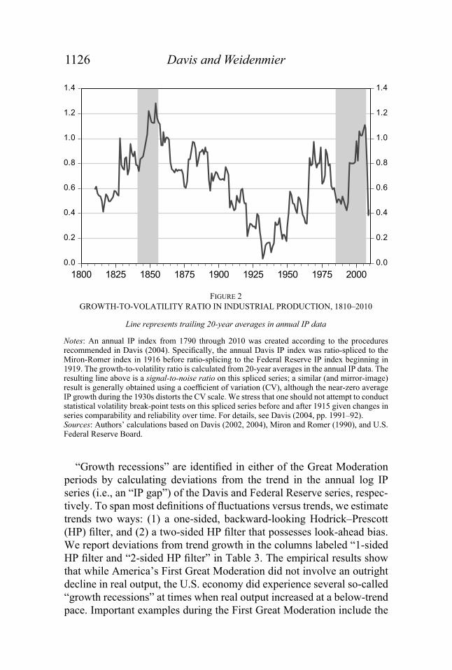
We examine the robustness of our identi cation of the First Great Moderation in two related ways. First, we judge how America’s Second (modern-day) Great Moderation looks using comparable annual IP uc-tuations. Second, we estimate Markov regime-switching models to assess the statistical signi cance of America’s First Great Moderation, and again compare those estimated results to same-frequency IP and stock-price data observed for the Second Great Moderation. We can get a general sense of the magnitudes of the two Great Moderations by creating trailing growth-to-volatility ratios in an annual IP index that spans both. We accomplish this by creating one extended annual IP series from 1790 through 2010 according to the procedures recommended in Davis (2004). Speci cally, we ratio-splice the annual Davis IP index to the Miron-Romer IP index in 1916 before ratio-splicing to annual values of the Federal Reserve IP index beginning in 1919. While we stress that we cannot conduct a formal statistical volatility break-point test on this long series given changes in series comparability and reliability over time, the growth-to-volatility ratio in Figure 2 allows us to visually gauge changes over rolling 20-year periods. Clearly, Figure 2 suggests that the combination of high IP growth and lower IP volatility during America’s rst Great Moderation appears to have been as impressive in scale as America’s second (modern-day) Great Moderation when measured against similar annual IP index data from the Federal Reserve.

We can also examine the business-cycle properties in the Second Great Moderation by dating recessions simply by declines in the annual IP index over the 1980–2010 period. As shown in the rst column of Table 3, recessions are denoted by parentheses which indicate a decrease in the IP index. The recessions of 1991, 2001, and 2008–2009 clearly show up in the Federal Reserve’s annual IP data.


“Growth recessions” are identi ed in either of the Great Moderation periods by calculating deviations from the trend in the annual log IP series (i.e., an “IP gap”) of the Davis and Federal Reserve series, respec-tively. To span most de nitions of uctuations versus trends, we estimate trends two ways: (1) a one-sided, backward-looking Hodrick–Prescott (HP) lter, and (2) a two-sided HP lter that possesses look-ahead bias. We report deviations from trend growth in the columns labeled “1-sided HP lter and “2-sided HP lter” in Table 3. The empirical results show that while America’s First Great Moderation did not involve an outright decline in real output, the U.S. economy did experience several so-called “growth recessions” at times when real output increased at a below-trend pace. Important examples during the First Great Moderation include the

0.0

0.2

0.4

0.6

0.8

1.0

1.2

1.4

0.0

0.2

0.4

0.6

0.8

1.0

1.2

1.4

1800 1825 1850 1875 1900 1925 1950 1975 2000

FIGURE 2GROWTH-TO-VOLATILITY RATIO IN INDUSTRIAL PRODUCTION, 1810–2010

Line represents trailing 20-year averages in annual IP data

Notes: An annual IP index from 1790 through 2010 was created according to the procedures recommended in Davis (2004). Speci cally, the annual Davis IP index was ratio-spliced to the Miron-Romer index in 1916 before ratio-splicing to the Federal Reserve IP index beginning in 1919. The growth-to-volatility ratio is calculated from 20-year averages in the annual IP data. The resulting line above is a signal-to-noise ratio on this spliced series; a similar (and mirror-image) result is generally obtained using a coef cient of variation (CV), although the near-zero average IP growth during the 1930s distorts the CV scale. We stress that one should not attempt to conduct statistical volatility break-point tests on this spliced series before and after 1915 given changes in series comparability and reliability over time. For details, see Davis (2004, pp. 1991–92).Sources: Authors’ calculations based on Davis (2002, 2004), Miron and Romer (1990), and U.S. Federal Reserve Board.

America’s First G

reat Moderation

1127TABLE 3

COMPARING THE TWO GREAT MODERATIONS USING ANNUAL IP DATA

Davis IP Index (Annual Frequency) Federal Reserve IP Index (Annual Frequency)

YearLog Growth Rate

(Percent) 1-sided HP Filter 2-sided HP Filter YearLog Growth Rate

(Percent) 1-sided HP Filter 2-sided HP Filter1830 16.81 3.27 (6.89) 1980 (2.58) (2.70) 1.181831 16.55 10.24 2.96 1981 1.33 (2.67) 0.751832 11.58 10.70 7.80 1982 (5.30) (6.66) (6.31)1833 10.85 9.67 12.10 1983 2.71 (3.56) (5.48)1834 (4.57) (1.60) 1.26 1984 8.53 2.41 1.011835 11.24 1.42 6.52 1985 1.20 1.35 0.041836 6.88 0.46 7.69 1986 1.00 0.44 (1.25)1837 (1.43) (5.50) 0.74 1987 5.04 2.40 1.371838 2.53 (6.33) (2.21) 1988 5.03 3.46 3.901839 12.37 (0.08) 4.55 1989 0.88 1.21 2.181840 (4.84) (7.06) (6.18) 1990 0.95 (0.29) 0.411841 5.47 (4.38) (7.06) 1991 (1.56) (2.82) (4.03)1842 2.78 (4.03) (11.22) 1992 2.79 (1.43) (4.36)1843 10.82 1.64 (7.98) 1993 3.21 (0.16) (4.51)1844 11.29 5.43 (4.86) 1994 5.15 1.90 (2.95)1845 9.47 6.26 (4.02) 1995 4.64 2.73 (2.05)1846 14.99 9.80 2.07 1996 4.35 2.86 (1.48)1847 14.03 10.67 7.17 1997 6.96 4.39 1.771848 8.26 6.69 6.65 1998 5.65 4.17 3.92

Davis and W

eidenmier

1128

TABLE 3 (CONTINUED)COMPARING THE TWO GREAT MODERATIONS USING ANNUAL IP DATA

Davis IP Index (Annual Frequency) Federal Reserve IP Index (Annual Frequency)

YearLog Growth Rate

(Percent) 1-sided HP Filter 2-sided HP Filter YearLog Growth Rate

(Percent) 1-sided HP Filter 2-sided HP Filter1849 3.56 0.62 1.73 1999 4.20 2.77 4.951850 4.04 (3.00) (2.36) 2000 3.94 1.49 6.121851 4.73 (4.64) (5.36) 2001 (3.47) (4.17) 0.331852 15.92 1.84 3.32 2002 0.21 (5.10) (1.38)1853 14.21 4.73 10.90 2003 1.26 (4.62) (1.67)1854 3.41 (0.70) 8.37 2004 2.30 (3.28) (0.56)1855 1.59 (5.27) 4.70 2005 3.19 (1.60) 1.771856 4.90 (5.65) 4.92 2006 2.17 (1.04) 3.441857 (1.48) (9.51) (0.80) 2007 2.63 (0.31) 5.891858 (5.54) (13.81) (10.34) 2008 (3.78) (3.91) 2.221859 13.51 (3.29) (0.79) 2009 (11.83) (11.04) (9.33)1860 1.73 (3.84) (3.05) 2010 5.15 (3.86) (3.86)

Notes: Hodrick-Prescott lters used lambda=100. Sources: Authors’ calculations based on data from Davis (2004) and U.S. Federal Reserve.


early 1840s following the Panic of 1839, as well as respites from other-wise strong growth in the late 1840s and the mid-1850s, periods that Thorp misclassi ed as recessions (Davis 2006). For the Second Great Moderation, similar growth recessions persist through roughly half of the 1984–2007 period. Using a one-sided real-time measure of devia-tion from trend, the U.S. economy did not grow above trend in any year between 2001 and 2010.

We estimate Markov regime-switching models to assess the statistical signi cance of changes in real economic volatility (high-vol, low-vol) before, during, and after the First Great Moderation using logarithmic growth rates in annual IP growth (1792–1914). We then compare our results to America’s Second Great Moderation using similar data and techniques for the post-WWII period. Our primary speci cation is a univariate autoregressive non-linear Markov-switching model with two regimes. In particular, we assume that annual IP growth, yt, depends on two underlying and unobserved states, Vt, t = 1,2 such that:

yt Vt Vt yt–1 t , t ~ N(0, Vt ). (1)

At rst pass, we allow the means, variances, and autoregressive param-eters to all vary between two states. We then also impose a constant-mean restriction based on the equality-of-means tests in Table 1, still allowing the variance and autoregressive parameters to vary between two states.

The Markov-model results for annual IP growth over the entire pre-WWI, 1792–1914 sample are reported in Table 4, Panel A. All esti-mated parameters are statistically signi cant at the 10 percent signi -cance level or better, with signi cant differences in volatility between the high-volatility and low-volatility states. Annual IP volatility in the low-volatility regime was approximately one-fourth that of high-volatility regime (0.27). The average mean growth rates estimated in the Markov-switching models is 4.29 percent per annum.12 Table 4 also compares the constant-mean results for the 1792–1914 period (Panel A) with those for annual IP data for the 1950–2010 period (Panel B). While the estimated standard deviation in the low-volatility state is marginally signi cant (p=0.12) in the later period, the standard deviation of the low-volatility state is almost 1/25th the size of the high-volatility state. The results from the Markov-switching model suggest that business cycle volatility was much less in the low-volatility state relative to the high volatility state, especially during the Second Great Moderation.

12 The empirical results are robust to using a switching mean growth speci cation. Details are available from the authors by request.

Davis and W

eidenmier

1130TABLE 4

MARKOV REGIME-SWITCHING MODELS FOR IP GROWTH

Panel A: Annual Sample, 1792–1914 Panel B: Annual Sample, 1950–2010State V1 State V2 State V1 State V2

(Low Volatility) (High Volatility) (Low Volatility) (High Volatility)

Variables

Estimate std error [p-value]

Estimate std error [p-value] Parameter



Mean growth ( ) 0.0429*** Mean growth ( ) 0.0226***0.0074 0.0051[0.00] [0.00]

Autoregressive term ( ) 0.4111*** (0.2605)* Autoregressive term ( ) 0.4772*** 0.01130.1061 0.1380 0.1024 0.1669[0.00] [0.06] [0.00] [0.95]

Standard deviation ( ) 0.0016*** 0.0057*** Standard deviation ( ) 0.0001 0.0030***0.0005 0.0011 0.0001 0.0006[0.00] [0.00] [0.12] [0.00]

Log-likelihood 158.25 Ratio ( 1 / 2) 0.27 Log-likelihood 103.88 Ratio ( 1 / 2) 0.04

* = Signi cant at the 10 percent level.** = Signi cant at the 5 percent level. *** = Signi cant at the 1 percent level.Notes: Model speci cation is an AR(1) switching-variance model with constant mean.Sources: Authors’ calculations and output from Markov-Regime Switching Model.


Panels A and B of Figure 3 show the low-volatility state probabili-ties from the Markov models for the Davis and Federal Reserve Board industrial production indices.13 Panel A of Figure 3 con rms that the First Great Moderation began in the early 1840s and ended in 1857, with the probability of a low-volatility state rising to nearly 90 percent in the late 1840s and early 1850s. The peak during the First Great Moderation is higher than at any other time during the 1792–1914 period. In a similar fashion, the probability of a low volatility state is highest during America’s Second Great Moderation. Again, the probability of a low-volatility state peaks during the mid to late 1990s and early 2000s.

Figure 4 compares the First Great Moderation with the Second Great Moderation by plotting the ratio of the conditional mean to the condi-tional standard deviation for the growth rate of the two industrial produc-tion series. The growth rate of the two IP series shows a spike in the ratio that coincides with a Great Moderation in the pre-WWI era as well as one in the modern era. By this metric the First and Second Great Moderations were very similar in relative magnitudes.14

SOURCES OF THE FIRST GREAT MODERATION IN INDUSTRIAL PRODUCTION

We hypothesize that a primary factor for the Great Moderation in both manufacturing and in the U.S. stock market was the diffusion of technologies centered in the transportation sector. Such technological diffusion would have generated spillovers in the form of increased investment, larger and more integrated product and labor markets, and increased western migration within the United States. Indeed, the First Great Moderation was characterized by the accelerated adoption of three important transportation and communication technologies: (1) the steam

13 The probability of a recession is calculated as the sum (p11+p21) of the probabilities having been in a high-vol state the previous year, p(11), or not p21. P21 is the probability of switching from a low volatility state to a high volatility state. The transition probabilities in this article are an example of a Markov Chain where the current state depends on the state of the previous year. Estimation of the transition probabilities is done by maximum likelihood estimation. The conditional probability density function for the observations of annual industrial production growth, yt given the state variables (high-vol and low-vol) and the previous observations (i.e.,

yt-1, yt-2,…) is de ned. The chain rule for conditional probabilities is then applied to derive the joint probability density function for yt, the state variables (high-vol and low-vol), and past information. The log-likelihood function is then maximized to estimate the recession probabilities.

14 We also estimated Markov-Switching models of monthly stock returns for the First and Second Great Moderation. The results basically con rm the ndings of the empirical analysis of the IP indices. The probability of being in a low volatility state was lower during the FGM and SGM. The results of the Markov-Switching models are robust to using a speci cation that allows for constant of switching mean growth rates.


locomotive and railroad, (2) faster clipper and steam ships, and (3) the telegraph.

According to George R. Taylor (1951), the 1840s and 1850s marked a “transportation revolution” in the antebellum U.S. economy that witnessed strong gains in productivity and high levels of investment.

FIGURE 3 LOW-VOLATILITY STATE PROBABILITIES FOR ANNUAL U.S. IP GROWTH RATES

Notes: Markov model’s low-volatility probabilities assume a constant mean. The lines are virtually identical for probabilities assuming a switching mean IP growth rate. Shaded areas are the periods of the First and Second Great Moderations. Source: Authors’ calculations.

Panel A: Davis IP Index, 1792–1914, for Markov switching-variance, switching AR(1) model

Panel B: FRB IP Index, 1950–2010 for Markov switching-variance, switching AR(1) model

0.0

0.2

0.4

0.6

0.8

1.0

0.0

0.2

0.4

0.6

0.8

1.0

1800 1810 1820 1830 1840 1850 1860 1870 1880 1890 1900 1910

0.0

0.2

0.4

0.6

0.8

1.0

0.0

0.2

0.4

0.6

0.8

1.0

1950 1960 1970 1980 1990 2000 2010


Trend economic growth was high in part due to high rates of both public and private investment in expanding transportation networks for roads, canals, railroads, and global shipping routes. During the 1840s and 1850s, American shipyards built more merchant tonnage than what was built in the previous four decades combined. Indeed, the zenith in merchant tonnage constructed in 1854 and 1855 would not be surpassed until WWI. Before the Civil War, the shipbuilding industry was large, representing more than 5 percent of the total value added in the indus-trial sector, exceeding the value added of locomotive production (3.6 percent weight in the Davis IP index). A primary factor in the surge in shipbuilding investment was the clipper ship, an extremely fast ship that possessed atter hulls, sharper bows and could routinely accommodate more than 2,000 tons in cargo. The discovery of gold in California in 1848 led to an immediate jump in the expected rates of return on fast ships that could quickly carry large cargoes to San Francisco and then sail to China (for its valuable tea). The fastest clipper ships built in the 1850s in the shipyards of New York, Boston, Philadelphia and Maine could cost nearly $3.13 million in current 2016 U.S. dollars to construct

0.5

0.6

0.7

0.8

0.9

1.0

0.5

0.6

0.7

0.8

0.9

1.0

1800 1825 1850 1875 1900 1925 1950 1975 2000

Markov model A:Pre-WWI sample, 1792-1914

Markov model B:Post-WWII sample, 1950-2010

FIGURE 4RATIO OF CONDITIONAL MEAN TO CONDITIONAL STANDARD DEVIATION IN

ANNUAL IP

Notes: Conditional means and standard deviations in each Markov regime-switching model were calculated based only on the ltered probabilities prior to time t. The Markov model was speci ed with switching volatilities and AR(1) terms but a constant mean; results are nearly identical with a switching-mean speci cation. Shaded regions demarcate America’s First and Second Great Moderations. Lines re ect centered 10-year moving averages in the ratio of conditional mean to conditional standard deviation.Sources: Authors’ calculations from the Markov-Regime Switching Model.


at the time, but they could sail from the eastern coast to San Francisco via the Cape Horn in as little as 90 days. One round-trip could net a pro t for ship owners equal to the entire cost of construction (Howe and Matthews 1986).15

The period from the late-1840s through the mid-1850s is gener-ally known as the “Clipper Ship Era.” The production of clipper ships increased from an index value of 58 in 1841 to a value of more than 158 in 1856. The period 1850 until 1856 represented the high point, an index value of 266 in 1854, for the clipper ship which bene tted from the gold rush in California and the China trade. Clipper ship production started to wane in 1857 as the clipper ship gradually gave way to steam powered ships that could carry heavier loads across the Atlantic and Paci c Oceans. The boom in clipper-ship construction had a signi cant economic impact on the U.S. lumber industry, with many coastal timber

elds being exhausted during the 1850s given the demand for lumber products to construct the large wooden ships. Steamship trade also expe-rienced a take-off during the First Great Moderation. The number of steamships involved in the Atlantic trade increased from 5,631 tons in 1847 to 97,296 tons in 1860 (Taylor 1951, p. 116).

Steam was also used to power rolling stock during the antebellum period. It took a few decades of innovation and capital investment before the railroad had a large impact on the antebellum economy. Rail mileage accelerated through the 1830s and 1840s, reaching 3,328 miles in 1840 and 8,879 by 1850. By 1850, railroad mileage had outpaced canals in 25 states. Both experienced an increase in tonnage in the West, but for water routes this was largely the result of massive Western migration, which increased demand across the board. This technological-diffusion process accelerated with the construction of almost 22,000 miles of track built in the 1850s. By the eve of the Civil War, railroads had replaced canals as the predominant means of transportation.16

To explore whether transportation played a critical role in America’s First Great Moderation, we created special sub-indices of the Davis IP series. We decompose the Davis IP index into two broad, mutually-exclusive sub-indices—an investment goods IP index and a consumption goods IP index. The investment goods index consists mostly of durable goods, including metal-producing sectors, transportation machinery,

15 We used the “simple” purchasing power calculator based on prices from the Measuring Worth website on eh.net to express the cost of building a clipper ship in current 2016 U.S. dollars (Williamson 2017).

16 For a discussion of the transportation revolution, see Fishlow (1965) and Atack and Margo (2009).


other small machinery categories, and the lumber industry. The consump-tion goods index consists of the food, textiles, printing, chemical/fuels, and leather-producing sectors.17 In 1850, the consumption goods industry accounted for approximately 60 percent of the total value added in the manufacturing and mining sectors, while manufacture of investment goods yielded the remaining 40 percent of industrial production.

We construct even ner-level IP indices from both the investment and consumption goods IP indices. For consumption goods, we create two IP indices—an IP food products index (accounting for 10.9 percent of the value-added in the industrial sector in 1850) and an IP textiles index (21.8 percent), which is primarily comprised of the cotton consumed by domestic textile mills. During this period, the textile sector was the largest industry on both a gross and value-added basis. For investment goods, we create an IP metals index (accounting for 12.9 percent of the value added in 1850) and an IP transportation-intensive index (22.7 percent) comprised of locomotive production, shipbuilding, and the primary input by far to ship construction at that time, lumber. Finally, we created an IP index excluding transportation-intensive sectors that accounts for the remaining series in the Davis IP index, accounting for 77.3 percent of that index on a value-added basis. We then calculate growth rates, standard deviations, and coef cients of variation for all of these IP series as we did for the aggregate index. The summary statistics are reported in Table 5. Several important features emerge. Both consumption and investment goods had higher rates of average growth during the Great Moderation than either before or after, although the boom in investment goods during the 1841–1856 period is much stronger, with growth in the transpor-tation IP index averaging 10 percent per annum versus only 3 percent per annum in the 1792–1840 period. The U-shaped pattern in volatility for the Davis IP index—lower volatility during the Great Moderation versus the periods before and after—is observed for investment goods, but not for consumption goods. The standard deviation in transportation-related production declines by one-third between the antebellum (0.179) and Great Moderation period (0.115) before nearly doubling in the post-bellum period (0.207). The decline in volatility in metals production is less pronounced and more monotonic throughout the 1828–1914 period.18

The combination of higher growth and even lower volatility for invest-ment goods leads to a pronounced U-shaped pattern in the coef cient of

17 These sector classi cations are similar to how the Federal Reserve today distinguishes between longer-term and generally more volatile durable-goods investment, and investment in and production of nondurable goods.

18 The IP metals index commences in 1827 given the limitations in pig-iron data.

Davis and W

eidenmier

1136TABLE 5

SUMMARY STATISTICS FOR IP COMPONENTS

Antebellum, pre-GM, 1792–1840 Great Moderation, 1841–1856 Postbellum, 1867–1914

All variables in log growth ratesMean

Growth (%)Standard Deviation


Mean Growth (%)

Standard Deviation


Mean Growth (%)

Standard Deviation


Davis IP index 4.65 0.067 1.45 7.66 0.050 0.65 4.61 0.075 1.63

IP, consumption goods 5.43 0.083 1.53 6.30 0.052 0.83 4.47 0.046 1.02 IP, food & agricultural products 4.34 0.252 5.80 4.23 0.158 3.72 4.40 0.067 1.53 IP, cotton textiles 6.09 0.149 2.45 6.94 0.161 2.32 4.69 0.106 2.25

IP, investment goods 3.71 0.154 4.15 9.66 0.078 0.81 4.81 0.127 2.65 IP, transportation 2.97 0.179 6.02 10.02 0.115 1.15 1.47 0.207 14.08 IP, metals 5.16 0.231 4.48 6.99 0.178 2.55 7.04 0.131 1.87

IP index, ex food products 4.81 0.085 1.77 8.12 0.052 0.63 4.64 0.085 1.82 IP index, ex textiles 4.33 0.090 2.07 7.82 0.047 0.60 4.61 0.078 1.70 IP index, ex transportation 5.57 0.080 1.44 6.96 0.063 0.91 5.10 0.063 1.24

Other annual variables

IP, U.K. 2.65 0.052 1.96 3.29 0.049 1.48 2.02 0.040 1.96 Wholesale prices –0.78 0.088 (11.30) 0.63 0.069 10.89 –1.17 0.057 (4.87) Cotton prices –2.96 0.229 (7.75) 1.27 0.227 17.83 –2.37 0.152 (6.41) Immigration rate 8.65 0.375 4.34 2.33 0.345 14.79 0.71 0.328 46.41

Tariff rate (%) 31.72 0.486 1.53 23.76 0.034 0.14 28.19 0.071 0.25 Cotton crop 11.79 0.185 1.57 4.73 0.186 3.92 4.40 0.191 4.34

Notes: All data expressed in logarithmic growth rates (except for tariffs) and are available back through 1792 except for IP metals (1828 with introduction of pig iron) and the immigration rate (1821). The IP index for consumption goods includes the Davis (2004, Table II, p. 1188) sector series for food products, textiles and apparel items, leather, printing and publishing, and chemical and fuel products. The IP investment goods index constitutes the remainder of the Davis IP index and includes metals, lumber, transportation equipment, and other small machinery categories (musical instruments, scienti c equipment, and ordnance).Sources: Authors’ calculations based on Davis (2002, 2004), Carter et al. 2006, Parts C and D, and NBER Macrohistory Database.


variation for the investment goods IP index. The coef cient of variation for investment goods is 0.81 for the Great Moderation, or 80 percent lower than for the earlier antebellum period (4.15) and nearly one-third lower than the post-bellum period (2.65). This U-shaped pattern in the coef cient of variation is even more striking for the transportation-goods sector, with a ratio of 1.15 during the Great Moderation, a fraction of that observed either before (6.02) or after the Civil War (14.08). Overall, the summary statistics in the top half of Table 5 would suggest that trans-portation-related investment contributed to the emergence of America’s First Great Moderation.

We test our hypothesis that transportation-related investment was the primary source of the recession-free period from 1841–1856. Again, we estimate the Markov regime-switching model on the IP indices that exclude textiles, transportation, and investment/consumption goods, respectively. In doing so, we can assess whether the exclusion of a primary sector (i.e., transportation or textiles) signi cantly weakens the proba-bility that the Great Moderation would have occurred. Figure 5 displays the probability that a series was in a low-volatility state for each year based on the Markov regime-switching model.19 Most notably, the Great Moderation is much weaker when one excludes transportation-goods investment, with only the 1843–1849 period possessing probabilities above 50 percent. The implication is that without transportation invest-ment, the U.S. economy would have only experienced a moderate expan-sion that ended before 1850 and would not have experienced the high growth of the 1850s. Second, the Great Moderation in investment goods is clearly evident in Figure 5; before 1841 the investment goods sector was rarely estimated to have been in a low-volatility state compared to the broader Davis IP index. Third, the results for the IP index excluding textiles in Figure 5 suggest that the Great Moderation may have persisted even longer had there not been more signi cant and negative impacts from the volatility in cotton textile production in the late 1850s.

The Markov-based results strongly suggest that the boom in trans-portation investment was a key contributor to America’s First Great Moderation. To better infer whether such investment spilled over to or led other economic activity, we run bivariate Granger-causality tests between each of the four key sectors (all investment goods, transporta-tion, metals, as well as textiles) on all other IP. We run these tests for the entire 1792–1914 sample, as well as for three sub-samples.20 First, we

19 The results of the Markov regime-switching model are reported in an Online Appendix.20 The Granger-causality tests are reported in an Online Appendix.


nd transportation IP led all other IP during the Great Moderation period at the 0.01 signi cance level, while all other IP did not lead uctuations in transportation production. Transportation IP statistically led growth in consumption-goods output, too, during the Great Moderation (p=0.03). Second, the results are exactly the opposite for textiles and metals, where all other IP led textile and metal IP during the Great Moderation at the

0.0

0.2

0.4

0.6

0.8

1.0

0.0

0.2

0.4

0.6

0.8

1.0

1830 1835 1840 1845 1850 1855 1860 1865 1870 1875 1880

Dav is IP indexIP, excluding transportation

0.0

0.2

0.4

0.6

0.8

1.0

0.0

0.2

0.4

0.6

0.8

1.0

1830 1835 1840 1845 1850 1855 1860 1865 1870 1875 1880

Dav is IP indexIP, excluding consumption goods (IP inv estment goods)

0.0

0.2

0.4

0.6

0.8

1.0

0.0

0.2

0.4

0.6

0.8

1.0

1830 1835 1840 1845 1850 1855 1860 1865 1870 1875 1880

Dav is IP indexIP excluding textile production

FIGURE 5PROBABILITIES OF LOW VOLATILITY STATES FOR IP WITH AND WITHOUT KEY

SECTORS

Notes: Figure does not show the entire 1792–1914 period to enhance clarity. Sources: Authors’ calculations from the Markov-Regime Switching Model.


0.02 and 0.05 signi cance levels, respectively. Third, growth in transpor-tation-related IP did not lead all other IP growth during the postbellum period; rather, the lead relationship ran in the opposite direction. We also tested whether the cotton crop, tariffs, or British IP lead changes in overall U.S. industrial production during the Great Moderation. The three variables did not Granger-cause the growth rate in the Davis indus-trial production series. Overall, the 1841–1856 period was unique in how the boom in transportation investment contributed to a period of higher growth and lower volatility.

CONCLUSION

The Great Moderation that commenced around 1984 is regarded by many economists as one of the longest periods of economic growth and low business cycle volatility in American history. In this article, we identify another, much earlier period of high economic growth and low economic and nancial market volatility. America’s First Great Moderation—a recession-free, 16-year period from 1841 until 1856—represents the longest economic expansion in U.S. history. The growth rate of industrial production was exceedingly high; annual growth in industrial production averaged nearly 8 percent per annum, the fastest pace of economic growth in the nineteenth century.

We believe that America’s antebellum “transportation revolution” was a signi cant driver of the First Great Moderation. We show that America’s First Great Moderation was largely driven by transportation-goods investment, which we attribute to the wider adoption of new tech-nologies for railroad and shipbuilding industries.

Markov regime-switching models reveal that the low-volatility derived for the First Great Moderation was of similar relative magni-tude and statistical signi cance to those estimated for the Second Great Moderation using comparable economic and stock-market data. This may make sense given several similarities between the 1841–1856 and 1984–2006 periods. Both moderations experienced a change in the struc-ture of the economy. The First Great Moderation witnessed the wide-spread adoption of new technologies—clipper and steam ships, railroads, and the telegraph—that helped contribute to signi cantly larger markets for goods, labor and exports. The modern Great Moderation saw struc-tural change in terms of the movement of production from goods to services, the IT revolution that led to better inventory management and

nancial innovations that allowed households and rms to better smooth consumption and investment. In addition, the rst and second modera-tions may have been characterized by improved economic policymaking.


Many states during the rst Great Moderation wrote new constitutions that rede ned the rules of the game for business and the government. As for the modern period, many scholars, including Ben Bernanke (2004), have argued that good monetary policy was an important factor in the Great Moderation from 1984–2007. Finally, both periods seem to have bene tted from good luck. While we do not observe signi cant changes in weather shocks or commodity prices during this period, it is likely that the rst Great Moderation bene tted from the discovery of gold in California. It also occurred during the era of Pax Britannica—a period of global peace (Brown et al. 2005) even though the United States fought in the Mexican-American War (1846–48). The second Great Moderation, on the other hand, appears to have been a period of generally low and stable oil prices coupled with few negative productivity shocks, at least up until 2007.

In summary, our analysis suggests that the First Great Moderation was characterized by high economic growth rates and low business cycle volatility. Like the modern-day Great Moderation, the end of America’s First Great Moderation was abrupt, pronounced, and notable for its magnitude following years of relative stability. Unlike the modern-day Great Moderation, however, America’s First Great Moderation occurred despite a low level of government spending, the absence of a central bank, and no marked improvement in price stability.

Ultimately, the ndings in our article may help alter not only how economic textbooks characterize the nineteenth-century economy, but today’s business cycle as well.

REFERENCES

Ahmed, Shaghill, Andrew Levin, and Beth Anne Wilson. “Recent U.S. Macroeconomic Performance: Good Policies, Good Practice, or Good Luck.” Review of Economics and Statistics 86, no. 3 (2004): 824–32.

Atack, Jeremy, Michael R. Haines, and Robert A. Margo. “Railroads and the Rise of the Factory: Evidence for the United States, 1850–1870.” NBER Working Paper No. 14410, Cambridge, MA, October 2008.

Atack, Jeremy, and Robert A. Margo. “Agricultural Improvements and Access to Rail Transportation: The American Midwest as a Test Case, 1850–1860.” NBER Working Paper No. 15520, Cambridge, MA, November 2009.

Bodenhorn, Howard. “Capital Mobility and Financial Integration in Antebellum America.” Journal of Economic History 52, no. 3 (1992): 585–610.

———. A History of Banking in Antebellum America: Financial Markets and Economic Development in an Era of Nation-Building. Cambridge: Cambridge University Press, 2000.


Bernanke, Ben. “The Great Moderation.” Remarks given at the meetings of the Eastern Economic Association. Washington, DC, 20 February 2004.

Berry, Thomas S. “Revised Annual Estimates of American Gross National Product: Preliminary Annual Estimates of 4 Major Components of Demand, 1789–1889.” Bostwick Paper No. 3, Richmond, VA, 1978.

Brown, William O., Richard C.K. Burdekin, and Marc D. Weidenmier. “Volatility in an Era of Reduced Uncertainty: Lessons from Pax Britannica.” Journal of Financial Economics 79, no. 3 (2006): 693–707.

Burns, Arthur F., and Wesley C. Mitchell. Measuring Business Cycles. New York: Columbia University Press, 1946.

Calomiris, Charles, and Christopher Hanes. “Consistent Output Series for the Antebellum and Postbellum Periods: Issues and Preliminary Results.” Journal of Economic History 54, no. 2 (1994): 409–22.

Calomiris, Charles, and Larry Schweikart. “The Panic of 1857: Origins, Transmission, and Containment.” Journal of Economic History 51, no. 4 (1991): 808–10.

Carter, Susan, Scott Gartner, and Michael Haines, et al., eds. Historical Statistics of the United States: Earliest Times to the Present, Millennial Edition. Parts A, C, and D. New York: Cambridge University Press, 2006.

Davis, Joseph. “A Quantity-Based Annual Index of U.S. Industrial Production, 1790–1915: An Empirical Appraisal of Historical Business-Cycle Fluctuations.” Ph.D. diss., Duke University, 2002.

———. “An Annual Index of US Industrial Production, 1790–1915.” Quarterly Journal of Economics 119, no. 4 (2004): 1177–215.

———. “An Improved Annual Chronology of U.S. Business Cycles.” Journal of Economic History 66, no. 1 (2006): 103–21.

Davis, Joseph, Christopher Hanes, and Paul W. Rhode. “Harvests and Business Cycles in Nineteenth-Century America.” Quarterly Journal of Economics 124, no. 4 (2009): 1675–727.

Davis, Lance E. “The New England Textile Mills and the Capital Markets: A Study of Industrial Borrowing 1840–1860.” Journal of Economic History 20, no.1 (1960): 1–30.

Fishlow, Albert. American Railroads and the Transformation of the Ante-bellum Economy. Cambridge: Harvard University Press, 1965.

Gallman Robert E. “Gross National Product in the United States, 1834–1909.” In Output, Employment, and Productivity in the United States after 1800, edited by Dorothy S. Brady, vol. 30, 3–76. NBER Studies in Income and Wealth. New York: Columbia University Press, 1966.

Goldin, Claudia, and Robert A. Margo. “Wages, Prices, and Labor Markets Before the Civil War.” NBER Working Paper No. 3198, Cambridge, MA, December 1989.

Goetzmann, William N., Roger G. Ibbotson, and Liang Peng. “A New Historical Database for the NYSE, 1815–1925: Performance and Predictability.” Journal of Financial Markets 4, no. 1 (2001): 1–32. Available online at http://icf.som.yale.edu/nyse/index.shtml.

Hammond, Bray. Banks and Politics in America: From the Revolution to the Civil War. Princeton: Princeton University Press, 1957.

Hobsbawm, Eric. Age of Capital: 1848–1975. London: Weidenfeld and Nicolson, 1975.


Hunt’s Merchant Magazine and Commercial Review. Vol. 28, p. 73. New York: 21 Fulton Street, 1853.

Irwin, Douglas A. “Antebellum Tariff Politics: Regional Coalitions and Shifting Economic Interests.” Journal of Law and Economics 51, no. 4 (2008): 715–42.

Jalil, Andrew. “A New History of Banking Panics, 1825–1929: Construction and Implications.” American Economic Journal: Macroeconomics 7, no. 3 (2015): 295–330.

Kindleberger, Charles P. Manias, Panics, and Crashes: A History of Financial Crises. New York: John Wiley and Sons, 2000.

Margo, Robert A. “Labor Market Integration before the Civil War.” NBER Working Paper No. 6643, Cambridge, MA, July, 1998.

———. “Regional Wage Gaps and the Settlement of the Midwest.” Explorations in Economic History 56, no. 2 (1999): 128–43.

McConnell, Margaret, and Gabriel Perez-Quiros. “Output Fluctuations in the United States: What Has Changed since the Early 1980s?” American Economic Review 90, no. 5 (2000): 1464–76.

Miron, Jeffrey A., and Christina D. Romer. “A New Monthly Index of Industrial Production, 1884–1940.” Journal of Economic History 50, no. 2 (1990): 321–32.

Moore, Geoffrey H., and Victor Zarnowitz. “The Development and Role of the National Bureau of Economic Research’s Business Cycle Chronologies.” In The American Business Cycle: Continuity and Change, edited by Robert J. Gordon, 735–79. NBER Studies in Business Cycles, vol. 25. Chicago: University of Chicago Press, 1986.

NBER Macrohistory Database. Cambridge, National Bureau of Economic History. http://www.nber.org/databases/macrohistory/contents/

Rhode, Paul W. “Gallman’s Annual Output Series for the United States, 1834–1909.” NBER Working Paper No. 8860, Cambridge, MA, April 2002.

Romer, Christina D. “Remeasuring Business Cycles.” Journal of Economic History 54, no. 3 (1994): 573–609.

Rostow, Walt W. The Stages of Economic Growth: A Non-Communist Manifesto. Cambridge, UK: Cambridge University Press, 1990.

Rousseau, Peter L. “Jacksonian Monetary Policy, Specie Flows, and the Panic of 1837.” Journal of Economic History 62, no. 2 (2002): 457–88.

Schwert, William G. “Indexes of United States Stock Prices from 1802 to 1987.” Journal of Business 63, no. 3 (1990): 399–426.

Smith, Walter B., and Arthur H. Cole. Fluctuations in American Business, 1790–1860. Cambridge, MA: Harvard University Press, 1935.

Stock, James H., and Mark W. Watson. “Has the Business Cycle Changed and Why?” NBER Macroeconomics Annual 17 (2002): 159–218.

Taylor, George R. The Transportation Revolution 1815–1860. New York: Rinehart & Co., 1951.

Temin, Peter. The Jacksonian Economy. New York: W. W. Norton & Company, Inc., 1969.

Temin, Peter. “Manufacturing.” In American Economic Growth, edited by Lance Davis et. al, 418–67. New York: Harper and Row, 1972.

Thorp, William L. Business Annals. Cambridge: NBER, 1926.


Turner, Frederick J. The Frontier in American History. New York: Henry Holt and Company, 1921.

Vandenbroucke, Guillaume. “The U.S. Westward Expansion.” International Economic Review 49, no. 1 (2008): 81–110.

Watson, Mark W. “Business-Cycle Durations and Postwar Stabilization of the U.S. Economy.” American Economic Review 84, no. 1 (1994): 24–46.

Williamson, Samuel H. “Purchasing Power of Money in the United States from 1774 to Present.” MeasuringWorth, 2017.

Zarnowitz, Victor. Business Cycles: Theory, History, Indicators, and Forecasting. NBER Studies in Business Cycles, vol. 27. Chicago: University of Chicago Press, 1992.

america’s first great moderation - cambridge.org · the journal of economic history, vol. 77, no....

Documents