[american institute of aeronautics and astronautics 7th aiaa atio conf, 2nd ceiat int'l conf on...

A Method for Assisting the Study of Pareto Solutions in Multi-Objective Optimization

J. Maginot1, M. Guenov2, P. Fantini3 and M. Padulo4

Cranfield University, Cranfield, MK43 0AL, UK

[Abstract] Solving a multi-objective optimization problem with conflicting objectives usually does not have a unique solution, but a set of non-dominated solutions referred to as Pareto points. For real industrial cases, the Pareto front cannot be obtained analytically and its description is often reduced to a set of discrete solutions. However, obtaining a single Pareto solution can be very time consuming and it is necessary for the designer to make the most out of any solution obtained without having to run more optimization procedures. In this paper, a strategy to save time and improve the efficiency of the trade-off decision-making process is presented. The proposed approach is to use global sensitivity analysis in order to reduce the dimensionality of the problem and local sensitivity analysis to study the adaptability of the Pareto solution. The results from a test case are presented and illustrate the potential of the approach.

Nomenclature

E(X) = expectation of random variable X f = objective function vector fi = objective function gi = constraint P = projection matrix Si

1 = first order sensitivity index of input variable xiSi

T = total sensitivity index of input variable xiV(X) = variance of random variable X X = random variable X = design space x = design vector xRed = reduced design vector of significant input variables xi = design variable Y = random variable Y = objective space y = objective vector yi = objective

1 PhD Student, Aerospace Engineering Department, Bldg. 83. 2 Professor, Aerospace Engineering Department, Bldg. 83. 3 PhD Student, Aerospace Engineering Department, Bldg. 83. 4 PhD Student, Aerospace Engineering Department, Bldg. 83.

American Institute of Aeronautics and Astronautics

1

7th AIAA Aviation Technology, Integration and Operations Conference (ATIO)<BR> 2nd Centre of E18 - 20 September 2007, Belfast, Northern Ireland

AIAA 2007-7792

Copyright © 2007 by the American Institute of Aeronautics and Astronautics, Inc. All rights reserved.

I. Introduction olving a multi-objective optimization problem with conflicting objectives usually does not have a unique solution, but a set of non-dominated solutions. Each of these is referred to as a Pareto solution. The set of all

non-dominated solutions in the objective space is called Pareto front and can be continuous, discontinuous, smooth or non-smooth. In the case of a real life multi-objective optimization problem (with highly non-linear objectives and constraints), the Pareto front cannot be obtained analytically and its description is often reduced to a set of discrete solutions. Furthermore, in the multi-objective optimization of a complex product such as aircraft where many disciplines are involved, obtaining a single Pareto solution can be very time consuming since the models used for the discipline analysis are called many times during the optimization process. It is therefore necessary for the designer to make the most out of any solution obtained without having to run more optimization procedures.

S

The objective of this work is to provide the designer with a strategy to improve the efficiency and effectiveness of the trade-off decision making process. Presented in this paper is a novel approach for exploring the Pareto set which combines a few features. A global sensitivity analysis is performed first in order to reduce the dimensionality of the complex optimization problem and gain some insight into the design space. Subsequently, a local sensitivity analysis of the Pareto front is used to study the sensitivity of the Pareto solution and local trade-offs between objectives. This process gives the decision maker more information on how to vary design parameters to adjust locally the criteria, with the assurance that no constraints will be violated in the vicinity of a candidate Pareto solution.

In the next section, the constituent features of the methodology are described. Section three contains an airfoil design test case demonstrating the approach. Finally, conclusions on the potential and applicability of the method are drawn.

II. Proposed Methodology

A. Formulation of the optimization problem An optimization problem is described in terms of a design variable vector x = (x1,x2,…,xN)T in the design space X

⊂ N. A function f ∈ M evaluates the quality of a solution by assigning it to an objective vector y = (y1,y2,…,yM)T where yi = fi(x), fi: N → 1, i = 1,2,….,M in the objective space Y ⊂ M. Thus, X is mapped onto Y by f: X|→Y. A multi-objective optimization problem may be formulated in the following form:

(2.1) min [ ( )]

xy x

Subject to L inequality constraints

g (x) 0i ≤ (2.2) = 1,...,i L

k

which may also include equality constraints. A constraint is said to be active if g ( x) = 0i

B. Global sensitivity analysis – Variance based methods Variance-based methods are rigorous and theoretically sound approaches for global sensitivity. The main idea is

to decompose the variance of a random output variable Y=Y(X) where X=(X1, X2,…,XN) is a vector of random input variables, into partial variances of increasing dimensionality1-4.

1,2,3,...,( ) ...i ij

i i jV Y V V V

≠

= + + +∑ ∑ (2.3)

where *[ ( / )]i iV V E Y X x= = i

−

(2.4)

* *[ ( / , )]ij i i j j i jV V E Y X x X x V V= = = − (2.5) and so on.

In the decomposition of the variance, the term Vi corresponds to the contribution to the output variance that is

only due to the variation of input Xi. The term Vij is the interaction effect between Xi and Xj. It represents the part of


2

the output variance due to variations of input parameters Xi and Xj, which cannot be explained by the sum of the first order effects of parameter Xi and Xj. Similar considerations can be made for higher order terms. Two coefficients of main interest for sensitivity can be defined:

- Main effect index: *

1 [ ( / )]( )

i ii

V E Y X xS

V Y=

=

- Total effect index: *( ) [ ( / )]

( )T i ii

V Y V E Y X xS

V Y− −− =

=

The main effect corresponds to the direct contribution of a variable to the variance of the output response while

the total effect represents its total contribution. For each input, the difference between the total effect and main effect gives an indication of the importance of the contribution to the output due to interactions with other inputs. Therefore, both main effect indices and total effect indices are necessary to obtain information about the non-additivity of the model and on the relative importance of variable interactions. Together, the main effect terms and total effect terms can provide a good description of the sensitivity of the outputs of the model under investigation.

When an analytical expression of the outputs in terms of the design variables is not available, numerical methods are used to compute estimates of the sensitivity indices. Two main methods have been developed: Sobol5-6 and FAST7 and have been implemented in the open source software SIMLAB8-9.

C. Reformulation of the optimization problem The results of global sensitivity analysis enable the designer to identify for each objective yi, i = 1,…,N the most

significant variables to the output variance. Input variables that are not significant to any objectives or constraints are removed from the formulation of the optimization problem by fixing them to a specific value. However, if an input variable is significant to at least an objective or a constraint, it must be retained as it could have a significant impact on the result of the optimization. After performing global sensitivity analysis, a new reduced design variable vector with only variables that appear to be significant to the optimization problem is defined and the optimization problem is re-formulated as follows:

redredmin [ ( )]

xy x (2.6)

Subject to L inequality constraints

redg ( ) 0i ≤x (2.7) = 1,...,i L

where xred is the reduced vector of significant input variables. The extent of the negligible contribution is to be decided by the designer, since by making such decision, he/she

has to compromise the quality of the optimization solutions obtained with the reduced optimization problem.

D. Obtaining approximation of the Pareto front A Pareto solution provides the designer with a feasible design where objective functions are compromised. However, no information on the vicinity of the solution and therefore its local sensitivity is available. In the case of the design of an aircraft, the designer might want to see whether the solution under study is flexible enough to be a suitable design. He/She might want to make sure that during the design process, a slight change in a requirement, for instance the improvement of one objective, will not result either in a disastrous reduction of the performance of one of the other objectives or in a drastic change of the design. Approximations of the Pareto surface10-11 have been derived and allow to study the local sensitivity analysis of a Pareto solution. Based on gradient projection method12-

13, they rely on the assumptions that the functions involved are differentiable and that the set of active constraints remains the same in the vicinity of the Pareto point that is investigated. The linear and quadratic approximations of the Pareto set are given as follows:


3

*

1

( 1, ..., ) fn

pp p i f

ii

dff f f p n M

df=

= + Δ = +∑ (2.8)

( )*

1 , 1

1 ( 1, ..., ) 2

f fn np p

p p i j k fjkii j k

dff f f H f f p n M

df= =

= + Δ + Δ Δ = +∑ ∑ (2.9)

where nf is the dimension of the largest family of linearly independent vectors P∇fi and P is the projection matrix onto the hyper-plane normal to all gradients of active constraints at the solution under study. In these equations,

p

i

dfdf

and2

( ) ppjk

j k

d fH

df df= are the first and second order derivatives on the Pareto surface10-11 and can be computed

from the usual gradients of objectives and active constraints, which are calculated during the optimization process. It shows that further information can be obtained at no extra computational cost. Equation (2.8) defines a hyperplane locally tangent to the Pareto surface. Similar local approximations for non-active constraints can be obtained and used to ensure that the new approximate Pareto solutions do not violate any constraints

*

1(1 ),,

f

k

nk

k ii i

k Ldg

g g fdf=

+ <= Δ∑ ≤ (2.10)

2

*

1 , 1.

12

f f

i j

n nk k

k k i i ji i ji

dg d gg g f f

df df df= == + Δ + Δ Δ∑ ∑ f (2.11)

Once a new approximate Pareto solution has been determined in the criterion space, the corresponding change in the design space can be mapped to obtain the new approximate design vector as follows:

1[( ) ]Td d d−= ≡ ∇ ∇ ∇x A f P f P f P f f (2.12) where is the matrix whose columns are the n∇P f f linearly independent vectors P∇fi.

III. Test Case – Airfoil optimization

A. Description of the test case The aforementioned approach was assessed on an airfoil optimization test case. PARSEC-11 parameterization14 was used to describe the airfoil as shown in Figure 1 (see also Table 2 for description of input parameters). The most attractive feature of this parameterization is the use of reduced number of intuitive and explicit geometric design parameters. Based on PARSEC-11 description, a Matlab script was written to generate the airfoil geometry.

Figure 1. PARSEC-11 airfoil parameterization


4

The aerodynamic features (Cd and Cm) of the airfoil were obtained using an ESDU code, VGK15-16, which has been developed for subsonic free streams and includes viscous and weak transonic effects. The FORTRAN code VGK was relatively fast to run and could be easily implemented in a Matlab environment for immediate use with an existing in-house developed optimization tool.

B. Kriging model for Cd and Cm The noise inherent to VGK in the estimates of Cd and Cm implies that any gradient-based method (optimization

or sensitivity analysis) will perform poorly as the output response is not smooth. Therefore, a surrogate model was built for both Cd and Cm. Another consequence is that it will also speed up the optimization procedure. The choice went for a Kriging model as it presents some attractive features for this test case. First, Kriging models are capable to accurately approximate complex functions and usually perform better than low order polynomial response surfaces17- -18 19. Then, the resulting output response will be noiseless, continuous and differentiable. Finally, their formulation allows to calculate analytically the sensitivity indices20 described previously.

A Kriging model is an interpolation model which expresses the realization of a deterministic process as the sum of the realization of a regression model and random function (stochastic process),

y ( ) ( )F z= +x x , (3.1)

where F is a low order polynomial and the random process z is assumed to have mean zero and covariance

2Cov( ( ), ( )) ( )i j i jZ Z = σx x x xR ,

)

(3.2)

where σ2 is the process variance. The correlation model R is defined by

=1

( ) ( x xN

i j i j

l l l ll

, ,= θ −∏x xR R . (3.3)

A variety of correlation functions is available but the most popular correlation model remains the Gaussian function17, ,20 21:

2( x x ) exp( (x x ) )i j i j

l l l l l l l,θ − = −θ −R , (3.4)

where the hyperparameters θl are optimized when fitting the Kriging model to the training sample. An appropriate design of experiments (DOE) strategy is necessary to obtain a suitable Kriging. Sequential designs18,21 usually perform much better than standard space filling designs. They are based on adding iteratively to the training sample, points of a design of experiment with large prediction error variance. Different techniques such as cross-validation and parametric bootstrapping can be used to select the candidate points18,21 but they become burdensome when the size of the sample increases. For this test case, a large number of points was required to obtain a sufficient description of Cd and Cm. Therefore these strategies were not appropriate. Instead, an alternative sequential strategy was adopted to ensure that training points were selected in regions that required a better description. In the proposed sequential strategy for fitting the Kriging model, an LP-Tau22 DOE of 4096 design points is first generated. The resulting design vectors are supplied to VGK to obtain the corresponding estimates for Cd and Cm. LP-Tau sequences are deterministic space-filling DOE that ensure uniform distribution of design points over the design space. Important feature of LP-Tau DOE is that larger LP-Tau sequences re-use points from smaller ones. From the total sample (4096 LP-Tau sequence), an initial training sample (256 LP-Tau sequence) is used to train the first Kriging model. The remaining points compose the test sample. As the Kriging models are to be used to predict outputs for the optimization, the Max error (3.5) over the test sample is preferred to the Mean Square Error (MSE) (3.6) as a measure of accuracy. Indeed, considering only an average value of the error could lead to erroneous solution of the optimization problem. In the case of a of a Kriging model, the max error on the total sample and on the test sample are the same as the model predictions for the points used for training are exact. Next, a set of new points with large max error is taken from the test sample and is added to the training sample. A minimum Euclidian distance is defined to ensure that the selected points are not clustered in the same region. The aim is to reduce the max error by adding selected points.


5

test sample

y yMax error ( )

yi i

i

| |max

| |

−= (3.5)

( i itest sampletest

2

1MSE = y y

n−∑ ) (3.6)

Then the new Kriging is fitted and its max error is compared with the previous one. If the max error has increased significantly, the new points are rejected and another set of points with large max error is taken from the test sample. The aim is to reduce the max error by adding selected points. Typically, we want:

new max error max error≤ γ × , (3.7) with γ < 1. We observe occasionally that adding such points might instead slightly increase the max error. Also, in this case, the training strategy experiences difficulties and takes longer to reach lower max error. Our experience shows that better results are achieved if γ is relaxed. For this problem, we used γ = 1.1. The sequential strategy adopted for fitting the Kriging model is described in Figure 2. .

Figure 2. Adaptive sequential strategy for Kriging model training


6

In this test case, DACE toolbox23-24 for Matlab was used to fit the Kriging model. The Gaussian function was chosen as it allows to calculate the sensitivity analysis indices analytically20. However, the choice of the regression model was not clear. Therefore, the adaptive sequential Kriging fitting described above was carried out for three regression models available in DACE toolbox, i.e constant, linear and quadratic. The history plot of max error and MSE during the sequential fitting procedure for Cd and Cm are given in Figure 3 and Figure 4, respectively. For this test case, the maximum training sample size was fixed to 1024. None of the Kriging models achieved the stopping criterion set to max error = 0.02.

Figure 3. Error history of Kriging model for Cd during adaptive training for different regression models

Figure 4. Error history of Kriging model for Cm during adaptive training for different regression models

The general tendency is that the max error and MSE decrease as the number of training points increases. Note that the curves for the MSE appear much smoother than the ones corresponding to the max error. This is a clear effect of the averaging of the error. For this test case, the quadratic regression model clearly outperforms both constant and linear regression models. The resulting Kriging models with quadratic regression and Gaussian correlation model are therefore used to predict the output values for Cd and Cm during the multi-objective optimization procedure. The max error and MSE for the final Kriging models when adaptive training reached the maximum training sample size of 1024 points are provided in Table 1.

Kriging - Cd Kriging - Cm

Regression model Max error MSE Max error MSE Constant 9.38e-02 2.05e-03 1.63e-01 5.37e-03 Linear 6.98e-02 1.06e-03 5.46e-02 4.36e-04

Quadratic 5.82e-02 3.73e-04 2.24e-02 1.11e-04

Table 1: Max error and MSE of Kriging models with different regression functions after adaptive training


7

C. Formulation of the optimization problem The design problem is to optimize the airfoil shape for 11 PARSEC input variables to minimize the total drag

and maximize the wing box volume: in the case of a 2-d airfoil, the area of the trapezoid defined by the position of the front and rear spars as shown in Figure 5.

Figure 5. Area of inner trapezoid box defined by front and rear spar

The optimization problem can be formulated as follows:

d1

12 602

Cymin

-area = -0.24*(t +t )y⎛ ⎞⎛ ⎞

= ⎜⎜ ⎟⎝ ⎠ ⎝ ⎠x % %

⎟

⎟

(3.8)

Subject to

m1

m2

123

604

C 0 07gC 0 04gt 0 076gt 0 072g

....

− −⎛ ⎞⎛ ⎞⎜ ⎟⎜ ⎟ +⎜⎜ ⎟ = ≤⎜⎜ ⎟ − +⎜ ⎟⎜ ⎟⎜ ⎟ ⎜ ⎟− +⎝ ⎠ ⎝ ⎠

0%

%

⎟ (3.9)

A description of the design variables and outputs considered in the optimization problem is given in Table 2. Here g1 and g2 are constraints on the achieved pitching moment while g3 and g4 are constraints on the thickness of the airfoil where the front and rear spar are positioned, respectively.

Inputs Description Outputs Description rle Leading edge radius Cd Total drag xup Upper surface max thickness location Cm Achieved pitching moment xlo Lower surface max thickness location area Area of trapezoid defined by front and rear spar zup Upper surface max thickness t12% Airfoil thickness at front spar position: 12% chord zlo Lower surface max thickness t60% Airfoil thickness at rear spar position: 60% chord zxxup Upper surface curvature at xup zxxlo Lower surface curvature at xlo zte Trailing edge position Δzte Trailing edge thickness βte Trailing edge aperture angle αte Angle of trailing edge bisector

Table 2: Description of model inputs and outputs for the optimization

The range of variations of the design parameters are given in Table 3 where the values for the bounds correspond to an airfoil with a reference chord of one meter.


8

Inputs Min value Max value rle (m) 0.005 0.00938 xup (m) 0.36 0.45 xlo (m) 0.3 0.56 zup (m) 0.045 0.057 zlo (m) -0.058 -0.04 zxxup (m-1) -0.555 -0.26 zxxlo (m-1) 0.28 1.1 zte (m) -0.02 -0.009 Δzte (m) 0.005 0.0082 βte (rad) 0.1 0.29 αte (rad) -0.13 -0.08

Table 3: Input range

For practical reasons, the input variables are scaled between -1 and 1 and if not specified, all design input values given in the following sections are the scaled ones.

The optimization is performed for a fixed lift coefficient, and specific Mach and Reynolds number as given in Table 4.

Flight conditions

Cl 0.71 Mach 0.72 Re 21e+06

Table 4: Optimization setting

D. Global sensitivity analysis of the model For the aerodynamic outputs, Cd and Cm, the exact first order and total sensitivity analysis indices are

analytically derived from the Kriging models20. The geometric outputs, i.e. the area, t12% and t60%, are obtained from the PARSEC-11 parameterization which does not require running the VGK code. Therefore, the first order and total sensitivity analysis indices for the area, t12% and t60% are obtained using the Sobol method implemented in SIMLAB8-

9 by running extensively the PARSEC-11 geometry generator. The first order and total sensitivity indices are given in Table 5 and Table 6 respectively.

First order indices Cd Cm area t12% t60%

rle 0.0912 0.0039 0.0144 0.0592 0.0015 xup 0.0320 0.0332 0.0018 0.0154 0.0232 xlo 0.0314 0.3737 0.0262 0.3360 0.4270 zup 0.1927 0.0954 0.1661 0.0628 0.1042 zlo 0.1240 0.1392 0.4117 0.1597 0.2542 zxxup 0.1030 0.0182 0.0370 0.0220 0.0165 zxxlo 0.0980 0.1824 0.3425 0.2806 0.1106 zte 0.0400 0.0566 0.0002 0.0003 0.0001 Δzte 0.0004 0.0016 0.0000 0.0001 0.0000 βte 0.0025 0.0033 0.0000 0.0020 0.0012 αte 0.0077 0.0461 0.0000 0.0000 0.0000

Table 5: First order sensitivity indices for Cd, Cm, area, t12% and t60%


9

Total order indices Cd Cm area t12% t60%

rle 0.1896 0.0055 0.0162 0.0602 0.0025 xup 0.1730 0.0365 0.0022 0.0169 0.0240 xlo 0.0462 0.4160 0.0279 0.3985 0.4878 zup 0.3740 0.0959 0.1660 0.0634 0.1036 zlo 0.1524 0.1400 0.4098 0.1574 0.2550 zxxup 0.1662 0.0208 0.0371 0.0227 0.0176 zxxlo 0.1205 0.2224 0.3424 0.3415 0.1694 zte 0.0655 0.0576 0.0011 0.0017 0.0002 Δzte 0.0010 0.0017 0.0001 0.0001 0.0001 βte 0.0045 0.0038 0.0009 0.0033 0.0013 αte 0.0103 0.0464 0.0003 0.0004 0.0000

Table 6: Total order sensitivity indices for Cd, Cm, area, t12% and t60%

A more intuitive visualization of the results is given in Figure 6 and Figure 7 where each bar indicates the total

contribution of each design variable to the output variance and is broken down into main effect and interaction effect. This bar chart representation gives an idea of the nature of the contributions and interactions between inputs.

Figure 6: Variance-based sensitivity analysis – Main and interaction effect for Cd and Cm

Figure 7: Variance-based sensitivity analysis – Main and interaction effect for area, t12% and t60%


10

Here we consider as non-significant, inputs with a total order index smaller than 0.02. It is clear that variables 9 and 10, i.e. Δzte and βte are non-significant and according to the methodology described in section 2 can be discarded from the optimization problem by fixing them to a specific value. The reduced optimization problem is formulated as follows:

red

d1

12 602

Cymin

-area = -0.24*(t +t )y⎛ ⎞⎛ ⎞

= ⎜⎜ ⎟⎝ ⎠ ⎝ ⎠x % %

⎟ (3.10)

Subject to

1 red m

2 red m

3 red 12

4 red 60

g ( ) C 0 07g ( ) C 0 04g ( ) t 0 076g ( ) t 0 072

....

− −⎛ ⎞ ⎛ ⎞⎜ ⎟ ⎜ ⎟+⎜ ⎟ ⎜ ⎟= ≤⎜ ⎟ ⎜ ⎟− +⎜ ⎟ ⎜ ⎟⎜ ⎟ ⎜ ⎟− +⎝ ⎠ ⎝ ⎠

xx

0xx

%

%

(3.11)

where

( )Tred le up lo up lo up lo te te te te r x x z z zxx zxx z z * *=x Δ β α (3.12)

with and constant. tez*Δ te*β

E. Pareto front The set of Pareto solutions of the reduced optimization problem is obtained for different values for Δzte and βte

using an in-house developed gradient-based optimization tool25. Table 7 provides information on the optimization procedure for three different runs. In the first run, all inputs are considered. In the two other runs, the optimization is performed on the reduced problem for two different combinations of values for Δzte and βte. When no information about the problem is available, common sense would fix Δzte and βte to their mean value. Therefore, for the first reduced optimization, Δzte and βte are set to zero. For the second reduced optimization, Δzte and βte have been fixed to their lower bound as a significant number of Pareto solutions of the full optimization problem correspond to these values.

All inputs Scaled Δzte = 0 / βte = 0 Scaled Δzte = -1 / βte = -1

Time 3h53min 2h11min 2h36min Function evaluations 314266 181997 219989 Pareto points obtained 201 167 221

Table 7: Performance comparison between different three optimization runs

It is clear that removing two inputs from the optimization procedure by fixing them to a specific value

considerably reduces the number of function evaluation and therefore the total computational time. It is a direct consequence of the reduction of the problem dimensionality. In the case of gradient optimization, less input variables implies that less effort is spent to obtain numerical estimates of gradient using finite differences.

The Pareto fronts corresponding to these three optimization runs are plotted in Figure 8. In this figure, the extreme values for Cd and area obtained on the 4096 LP-Tau DOE are taken as the bounds of the x and y axes. Figure 8 clearly shows that all Pareto fronts are located in the same region. It is important to notice that the extent of the range of variation for Cd and for the area remains the same. The Pareto front, where Δzte and βte are fixed to zero, shows good agreement with the solutions of the full problem for values of Cd up to 0.0098, but fails to do so for higher values. It can be explained by the fact that for solutions of the full problem that correspond to values of Cd higher than 0.0098, the constraints on the minimum values for Δzte and βte are active. As it could be expected, the solutions obtained, when Δzte and βte are fixed to -1, show a better match with this part of the Pareto front obtained for the full problem.


11

Reducing the dimensionality of the optimization problem by freezing non-significant variables to a specific value might come at the expense of the quality of the Pareto front. Indeed, some parts of the Pareto surface are not captured accurately by the reduced problem. Therefore, when the designer decides to reduce the number of variables using this approach he/she must be aware that the quality of the resulting Pareto surface might be compromised.

Figure 8: Pareto surface obtained for the two-objective airfoil optimization problem

F. Pareto approximation In this section, we focus on the use of local approximations of the Pareto surface to understand the trade-offs

between objectives and the adaptability of a Pareto solution. Figure 8, shows that all Pareto solutions are located in a specific region of the criterion space but the

discontinuities in the Pareto surface seems to indicate that they correspond to different type of airfoils. Figure 9 shows the location in the criterion space of a few representative Pareto solutions. The corresponding airfoils are plotted in Figure 10. It gives an idea of the diversity of the Pareto solutions lying on the Pareto surface.

Figure 9: A few characteristic solutions in the criterion space


12

Figure 10: A few characteristic Pareto solution airfoils

In this test case, a good description of the Pareto surface is given as a significant number of Pareto points can be obtained at an affordable computational cost. However, when high fidelity codes are used in place of surrogate models, obtaining a single Pareto solution could be very demanding and the designer will benefit from obtaining information about the local sensitivity analysis of the candidate solution.

When a candidate Pareto solution is obtained, the linear and quadratic approximations can be derived from (2.8) and (2.9). For a small change in one objective, the local trade-off in the other objective can be computed and the corresponding change in the design space can be obtained using (2.12). In this context, the range of validity of the local approximation is not clear. It is proposed to use the difference between quadratic and linear prediction to measure the extent of the validity of the approximation10-11. When the contribution of the quadratic term becomes too important with respect to the linear term, the linear approximation is not considered reliable. Meanwhile, the designer must ensure that all constraints from the optimization problem are still satisfied. In other words, in the case of a two objective optimization problem, to assess the extent of the validity of the linear approximation, the designer must solve a double linear optimization problem:

Minimize and maximize 1d f

Subject to

1 d 1− ≤ + ≤x x , (3.13)

1

1

dd

df

f+ ≤

gg 0 , (3.14)

2

2 212

1 1

d d1d

2 d d

f ff

f f≤ α . (3.15)

The first two equations impose that constraints on the design variables range and that the other constraints (3.9) are still satisfied. Equation (3.15) requires that the contribution of the quadratic term remains smaller than a fraction of the linear term. It allows to detect when the curvature becomes important and where the Pareto surface departs from the linear approximation. The scalar α is defined by the designer and represent the relative contribution of the quadratic term with respect to the linear one.


13

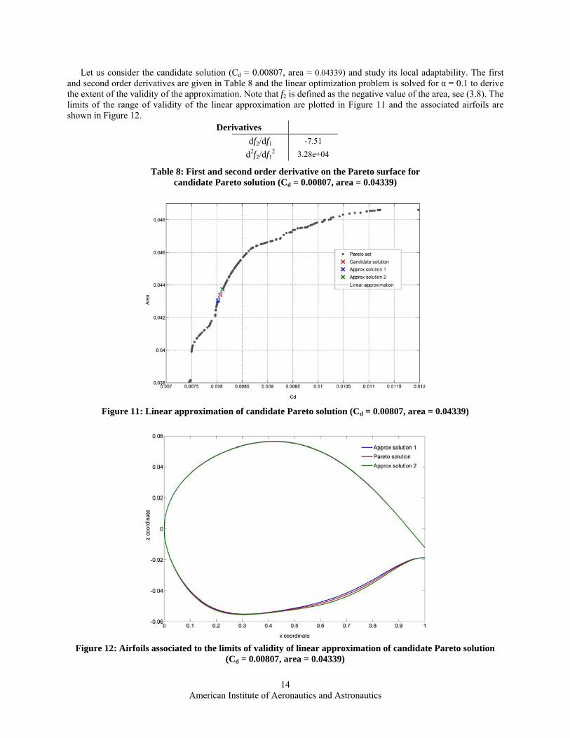
Let us consider the candidate solution (Cd = 0.00807, area = 0.04339) and study its local adaptability. The first and second order derivatives are given in Table 8 and the linear optimization problem is solved for α = 0.1 to derive the extent of the validity of the approximation. Note that f2 is defined as the negative value of the area, see (3.8). The limits of the range of validity of the linear approximation are plotted in Figure 11 and the associated airfoils are shown in Figure 12.

Derivatives df2/df1 -7.51 d2f2/df1

2 3.28e+04

Table 8: First and second order derivative on the Pareto surface for candidate Pareto solution (Cd = 0.00807, area = 0.04339)

Figure 11: Linear approximation of candidate Pareto solution (Cd = 0.00807, area = 0.04339)

Figure 12: Airfoils associated to the limits of validity of linear approximation of candidate Pareto solution

(Cd = 0.00807, area = 0.04339)


14

It is clear that along the direction given by the linear approximation, approximated Pareto airfoils differ mainly in their lower surface. The corresponding values for their inputs, objectives and constraints are given in Table 9. The output values predicted by the approximation show good agreement with those obtained with the model. The linear approximation provides the designer with an insight in the Pareto solution that can be found in this region of the criterion space.

Approx solution 1 Pareto solution 1 Approx solution 2 rle 0.06400 0.06521 0.06641 xup 0.37032 0.37263 0.37493 xlo -0.91566 -0.94435 -0.97303 zup 0.90145 0.91516 0.92887 zlo -0.67471 -0.69336 -0.71202 zxxup 0.16030 0.16645 0.17260 zxxlo -0.81905 -0.83604 -0.85303 zte -0.16488 -0.16715 -0.16942 Δzte 0.04200 0.04235 0.04270 βte -0.09983 -0.09997 -0.10011 αte 0.01455 0.01341 0.01227 Approx Model Model Approx Model Cd 0.00802 0.00802 0.00807 0.00811 0.00812 area 0.04305 0.04306 0.04339 0.04374 0.04375 g1 0.00000 0.00032 0.00000 0.00000 0.00029 g2 -0.03000 -0.03032 -0.03000 -0.03000 -0.03029 g3 -0.00617 -0.00617 -0.00663 -0.00708 -0.00708 g4 -0.02520 -0.02524 -0.02617 -0.02715 -0.02719

Table 9: Inputs, objectives and constraints values of candidate Pareto solution (Cd = 0.00807, area = 0.04339) and approximated Pareto solutions associated to

limits of validity of linear approximation

For candidate Pareto solution (Cd = 0.00807, area = 0.04339), the range of validity of the linear approximation is limited by constraint (3.15) related to the departure of the Pareto surface from its local tangent. Table 9 shows that no other constraint is activated. It results that the range of validity of the linear approximation is centered on the candidate Pareto solution. Let us consider a different candidate solution (Cd = 0.00837, area = 0.04512) and carry out a similar analysis. First, the first and second order derivatives are obtained and given in Table 10. For this candidate solution, the trade-off between objectives is clearly less important than for the first candidate solution.

Derivatives df2/df1 -4.35 d2f2/df1

2 9.01e+03

Table 10: First and second order derivative on the Pareto surface for candidate Pareto solution (Cd = 0.00837, area = 0.04512)

As for the first Pareto candidate, the linear optimization problem is solved for α = 0.1 to derive the extent of the validity of the approximation. For this candidate Pareto solution, the minimum value for df1 is limited by the constraint on the quadratic term (3.15) while the maximum value for df1 is limited by a constraint on the range of variation of x (3.13) which becomes active first. It results that the range of the validity of the linear approximation is not centered on the candidate Pareto solution as shown in Figure 13. It illustrates that all constraints must be taken into account when estimating the extent of validity of the local approximation since for a candidate Pareto solution,


15

inactive constraints might be close to become active. The associated airfoils are given in Figure 14 and show that the changes in the airfoil geometry for the approximated Pareto solutions are very small.

Figure 13: Linear approximation of candidate Pareto solution (Cd = 0.00837, area = 0.04512)

Figure 14: Airfoils associated to the limits of validity of linear approximation of candidate Pareto solution

(Cd = 0.00837, area = 0.04512)

The corresponding values for their inputs, objectives and constraints are given in Table 11. Similar to the first candidate Pareto solution, the values of the outputs obtained with the linear approximation for the new approximated Pareto solution match the values obtained with the model. As mentioned before, for the second approximated solution, variable zup reaches its maximum value (zup = 1).


16

Approx solution 1 Pareto solution 2 Approx solution 2 rle 0.07227 0.07590 0.07744 xup 0.39724 0.41098 0.41678 xlo -1.00000 -1.00000 -1.00000 zup 0.92966 0.97911 1.00000 zlo -0.77073 -0.81022 -0.82691 zxxup 0.19328 0.21416 0.22298 zxxlo -0.95874 -0.98073 -0.99002 zte -0.26966 -0.28366 -0.28958 Δzte 0.10616 0.10855 0.10955 βte -0.21414 -0.21912 -0.22122 αte -0.10551 -0.11622 -0.12075 Approx Model Model Approx Model Cd 0.00827 0.00828 0.00837 0.00841 0.00841 area 0.04469 0.04469 0.04512 0.04529 0.04529 g1 0.00000 0.00005 0.00000 0.00000 0.00001 g2 -0.03000 -0.03005 -0.03000 -0.03000 -0.03001 g3 -0.00803 -0.00803 -0.00856 -0.00878 -0.00879 g4 -0.03020 -0.03020 -0.03142 -0.03194 -0.03194

Table 11: Inputs, objectives and constraints values of candidate Pareto solution (Cd = 0.00837, area = 0.04512) and approximated Pareto solutions associated to

limits of validity of linear approximation

IV. Conclusions Presented is a novel method for helping the designer investigate solutions of a multi-objective optimization problem. It includes global and local sensitivity components: the former aims to reduce the dimensionality of the search space to reduce the number of calls to computationally expensive analyses and the latter aims to obtain local information at a candidate Pareto solution without running further optimization. The use of global sensitivity on a multi-objective optimization airfoil design seems promising as it enables to reduce significantly the computational effort. However, it comes at the expense of a slight reduction in the quality of the solutions obtained. The approach would benefit from a method that would help the designer decide on the most appropriate specific value to fix non-significant variables. Local approximations of the Pareto surface for a candidate solution provide information on other Pareto solutions that can be found in its vicinity. Ultimately, this process gives the decision maker more information on the way to vary design parameters to adjust locally the criteria to suit his/her preferences, with the assurance that no constraints will be violated in the vicinity the candidate Pareto solution. The results obtained on the airfoil design test case show potential for this approach to assist the decision-maker in the process of trade-off analysis.

Acknowledgments The research reported in this paper has been carried out within the VIVACE Integrated Project (AIP3 CT-2003-

502917) that is partly sponsored by the Sixth Framework Programme of the European Community (2002-2006) under priority 4 “Aeronautics and Space”. The authors gratefully thank Peter Coleman, Dr. Carren Holden and Ilya Tolchinsky from Airbus UK, for their contribution to the development of the test case.


17

References 1 Campolongo, F., Tarantola, S., and Saltelli, A., “Tackling Quantitatively Large Dimensionality Problems,” Computer

Physics Communications, Vol. 117, 1999, pp. 75-85. 2 Saltelli, A., Andres, T. H., and Homma, T., “Sensitivity Analysis of Model Output: An Investigation of New Techniques,”

Computational Statistics & Data Analysis, Vol. 15, 1993, pp. 211-238. 3 Saltelli, A., Chan, K., and Scott, M., Sensitivity Analysis, New York, John Wiley & Sons, Edition 2000. 4 Saltelli, A., Tarantola, S., and Chan, K. P. S., “A Quantitative Model-Independent Method for Global Sensitivity Analysis

of Model Output,” Technometrics, Vol. 41, No. 1, 1999, pp. 39-56. 5 Sobol’, I. M., “Global Sensitivity Indices for Non-Linear Mathematical Models and their Monte Carlo Estimates,”

Mathematics and Computers in Simulation, 55, 2001, pp. 271-280. 6 Sobol’, I. M., “Sensitivity Analysis for Non-Linear Mathematical Models,” Mathematical Modeling & Computational

Experiments, 1993, Vol. 1, No. 4, pp. 407-414. 7 Saltelli, A., and Bolado, R., “An Alternative Way to Compute Fourier Amplitude Sensitivity Test (FAST),” Computational

Statistics & Data Analysis, Vol. 26, 1998, pp. 445-460. 8 Saltelli, A., and Tarantola, S., SimLab 2.2, Reference Manual, European Commission - Institute for the Protection and

Security of the Citizen (IPSC). 9 Saltelli, A., Tarantola, S., Campolongo, F., and Ratto, M., Sensitivity Analysis in Practice, John Wiley & Sons, 2004. 10 Utyuzhnikov, S.V., Maginot, J., and Guenov, M., “Local Pareto Analyzer for Preliminary Design,” Proceedings of the 25th

International Congress of the Aeronautical Sciences, ICAS, Stockholm, Sweden, 2006. 11 Utyuzhnikov, S.V., Maginot, J., and Guenov, M., “Local Approximation of Pareto Surface,” Proceedings of the World

Congress on Engineering, Vol. 2, IAENG, Hong Kong, 2007, pp. 898-903. 12 Zhang, W.H., “On the Pareto Optimum Sensitivity Analysis in Multicriteria Optimization,” International Journal for

Numerical Methods in Engineering, 58, 2003, pp. 955-977. 13 Zhang, W.H., “Pareto sensitivity analysis in multi-criteria optimization,” Finite Elements in Analysis and Design, 39, 2003,

pp. 505-520. 14 Sobieczky, H., “Parametric Airfoils and Wings,” Notes on Numerical Fluid Mechanics, Vol. 68, 1998, pp. 71-88. 15 ESDU 96028, “VGK method for two-dimensional aerofoil sections. Part I: Principles and results,” April 2004. 16 ESDU 96029, “VGK method for two-dimensional aerofoil sections. Part II: User manual for operation with MS-DOS and

UNIX systems,” April 2004. 17 Simpson, T. W., Lin, D. K. J., and Chen, W., “Sampling Strategies for Computer Experiments: Design and Analysis,”

International Journal of Reliability and Applications, Vol. 2, 2001, pp. 209-240. 18 Van Beers, W. C., M. and Kleijnen, J. P. C., “Kriging Interpolation in Simulation: A Survey,” Proceedings of the 2004

Winter Simulation Conference, IEEE Press, 2004. 19 Donald, R. J., Matthias S., and William, J. W., “Efficient Global Optimization of Expensive Black-Box Function,” Journal

of Global Optimization, Vol. 13, 1998, pp. 455-492. 20 Chen, W., Jin, R., and Sudjianto, A., “Analytical Variance-Based Global Sensitivity Analysis in Simulation-Based Design

Under Uncertainty,” Journal of Mechanical Design, Vol. 127, 2005, pp. 875-886. 21 Martin, J. D., and Simpson, T. W., “Use of Adaptative Metamodeling for Design Optimization,” Proceedings of the 9th

AIAA/ISSMO Symposium on Multidisciplinary Analysis and Optimization, AIAA, Washington, 2002. 22 Statnikov, R. B., and Matusov, J. B., Multicriteria Analysis in Engineering, Kluwer Academic Publishers, 2002. 23 Lophaven, S., Nielsen, H., and Sondergaard, J., “DACE – A Matlab Kriging Toolbox,” Technical report IMM-TR-2002-12,

Technical University of Denmark, 2002. 24 Lophaven, S., Nielsen, H., and Sondergaard, J., “Aspects of the Matlab toolbox DACE,” Technical report IMM- REP-

2002-13, Technical University of Denmark, 2002. 25 Fantini, P., Balachandran, L. K., and Guenov, M. D., “Computational Intelligence in Multi Disciplinary Optimization at

Feasibility Design Stage,” First International Conference on Multidisciplinary Design Optimization and Applications, ASMDO, Besançon, France, 2007.


18

[american institute of aeronautics and astronautics 7th aiaa atio conf, 2nd ceiat int'l conf on...

Documents