[american institute of aeronautics and astronautics 48th aiaa/asme/asce/ahs/asc structures,...

American Institute of Aeronautics and Astronautics

1

System-level Optimization and Concurrent Engineering:

A Comparative Experiment

Brian K. Bairstow* Jet Propulsion Laboratory, Pasadena, California, 91109

Olivier de Weck† Massachusetts Institute of Technology, Cambridge, Massachusetts, 02139

and

Jaroslaw Sobieszczanski-Sobieski‡ NASA Langley Research Center, Hampton, Virginia, 23681-2199

One method for rapid conceptual design is integrated concurrent engineering. This

generally involves a team of designers manually exploring a design space, while attempting

to satisfy all requirements. By including system-level optimization techniques in the

integrated concurrent engineering process, it is possible to improve the efficiency and results

of the design process. This experimental study was performed to confirm and quantify those

improvements. A two-stage liquid rocket model was used as the focus of the study. This

model represented a complex and coupled multidisciplinary design problem in which several

input parameters could be varied to affect the outputs of rocket performance and cost.

Several design teams were given the task of optimizing the rocket by simultaneously

maximizing mass capability and minimizing cost. Some of the design teams used system-

level optimization in parallel with integrated concurrent engineering, while the other teams

used integrated concurrent engineering only. The results of the design sessions were

compared with respect to several metrics, and it was shown that optimization shows

significant advantages, with over 90% confidence in certain categories.

Nomenclature

Afinal = ending altitude, km Astage = staging altitude, km C = total cost, $ m0 = initial wet mass, kg mengine = engine mass, kg mp = payload mass, kg Rr = rocket radius, m T1...T5 = thrust profile parameters, N

α1, α2 = thrust angle profile parameters, rad

νa = first axial mode frequency, Hz νb = first bending mode frequency, Hz

* Engineering Associate, Mission Concepts Section 312, 301-180, AIAA Student Member, [email protected]. This work was performed prior to involvement with JPL, while a graduate student in the Department of Aeronautics and Astronautics at MIT. † Associate Professor of Aeronautics and Astronautics and Engineering Systems, Department of Aeronautics and Astronautics, 33-410, AIAA Associate Fellow, [email protected]. ‡ Senior Research Scientist, Computation Structures and Materials Branch, AIAA Fellow, [email protected]

48th AIAA/ASME/ASCE/AHS/ASC Structures, Structural Dynamics, and Materials Conference<br> 15th23 - 26 April 2007, Honolulu, Hawaii

AIAA 2007-1879

Copyright © 2007 by Brian Bairstow. Published by the American Institute of Aeronautics and Astronautics, Inc., with permission.


2

θc = cone half-angle, rad ICE = Integrated Concurrent Engineering MDO = Multidisciplinary Design Optimization MOGA = Multi-Objective Genetic Algorithm

I. Introduction

HE problem of multidisciplinary engineering design is by nature a difficult one. Complex relationships and interdependencies combined with a multidimensional design space can make it challenging to gain traction on a

design problem. Furthermore, the most basic decisions that define form and function must be made at the beginning of the engineering process, when there is the smallest amount of experience and knowledge. Several techniques have been developed to facilitate the engineering design process. Concurrent engineering is the process of bringing engineers to work together in face-to-face design sessions. This has the value of increasing communication to avoid problems and misconceptions. This also avoids the scenario in which people meet to discuss a problem, work separately back in their offices, and then meet again a week later, which can be inefficient. Integrated concurrent engineering (ICE) is a logical extension of the concurrent engineering processes in which the tools and calculations of the individuals are linked together, via a computer network for example, in order for rapid exchange of information and numbers to occur. Another process for aiding design is system-level multidisciplinary optimization. These methods take advantage of the ever-increasing computational power available to vary input parameters across several subsystems to optimize the outputs of the entire system. An example is the optimization of the shape and thrust profile of a rocket to maximize the payload mass capacity while minimizing the cost. There is potential for benefits to be reaped by combining the processes of integrated concurrent engineering and system-level multidisciplinary optimization using the methodology of Multidisciplinary Design Optimization (MDO). While the MDO literature has grown tremendously in breadth and depth during the recent decades, there is a conspicuous lack of studies to assess advantages of MDO over traditional practices.1 One attempt for such assessment was by Schuman et al and the work reported herein is a sequel to that attempt.2-3 The Schuman et al study explored the MDO advantages by comparing integrated concurrent design of the Space Shuttle external fuel tank with and without optimization as a tool.2-3 The results showed a slight improvement when including optimization, but were not conclusive. This was in part so because the external fuel tank problem was so simple (6 design variables, few constraints, and low to moderate coupling in the system) that the human design team, without the assistance of system optimization in the background, was able to intuit the best portions of the objective space in a typical 2 hour design session. This study extends that work into more trials and with a more difficult design problem in order to assess benefits from including system-level optimization more conclusively. The metrics for this comparison relate to efficiently populating a wide Pareto front of good designs.

II. Model and Optimization

The model used was a two-stage, liquid rocket model developed for this purpose, and is described in greater detail in a previous paper.4 The model was simplified consistent with the resources available for the study. The basic geometric structure used in the rocket model is depicted in Figure 1. The rocket has a cylindrical body capped with a cone. The rocket dimensions are determined by the radius Rr and the length of the propellant tanks. The propellant tanks hold the oxidizer and fuel, and are cylinders capped with hemispheres.

There are two objective outputs from the model: payload mass and cost. The payload mass should be maximized and the cost minimized. There are three more outputs that act as constraints, the ending altitude, which must not be less than the target altitude of 400 km, and the frequencies of the first axial and bending modes of vibration. There are fifteen inputs to the system which comprise the design vector. These design variables are the initial wet mass, the rocket cylinder radius, the

T

Figure 1. Rocket design diagram.


3

half-angle of the nose-cone, five parameters describing the thrust profile over altitude, two parameters describing the thrust-angle profile over altitude, the altitude at which to stage, the propellant types to use in stage one and stage two, and the structural materials used in the rocket body and tanks. The objectives, constraints, and design variables are listed in Table 1.

Table 1. Input and objective variables.

Name Symbol Unit Description

Objectives

payload mass mp [kg] objective

cost C [$] objective

Constraint Outputs

ending altitude Afinal [km] constraint

axial mode freq. νa [Hz] constraint

bending mode freq. νb [Hz] constraint

Design Vector

initial wet mass m0 [kg] design variable

rocket radius Rr [m] design variable

cone half-angle θc [rad] design variable

thrust profile T1...T5 [N] design variable

angle profile α1, α2 - design variable

staging altitude Astage [km] design variable fuel type – stage 1 - design variable

fuel type – stage 2 - design variable

structure material - design variable

tank material - design variable

The model has fifteen inputs and couplings between the trajectory, propulsion, and structures subsystems. These

make the problem more complex than the Space Shuttle external fuel tank problem used previously and more than doubles the number of design variables.2-3 This increase in complexity makes it a more difficult design problem to tackle, largely due to the notion that it is difficult for humans to deal with more than about seven things at a time.5

The system-level optimizer chosen was a multi-objective genetic algorithm (MOGA).6 This heuristic technique was chosen because discrete design variables such as material type and propellant type were used, and genetic algorithms handle discrete variables well. The two objectives were to maximize payload mass and minimize cost.

The implementation of the optimization and analysis of the results applied to the rocket model are described in previous work.4 The optimizer was deemed suitable for this study. After generating a population of size 100, 100 generations were run with about a five minute run time (each), the code built a Pareto front approximation from the non-dominated feasible designs. A design, X, is dominated if there is another feasible design, Y, for which all objectives are improved over X (both a lower cost and a higher payload mass), and X is non-dominated if no such point Y exists.

Below are examples of the output from the genetic algorithm. Figure 2 shows all the feasible design points from a 100 generation run. Typically of the 10,000 individuals from a run, 2000-4000 will represent feasible designs. Figure 3 shows the non-dominated solutions from Figure 2. The utopia point is to the lower right, with a high payload of 50.7 tons and a low (per unit) cost of 140.2 $M. The utopia point is the design whose objectives are at their respective best obtained by single objective optimizations.


4

Notice that the Pareto front made is not very well distributed and has discontinuities. Running the MOGA

multiple times would lead to covering different ranges and help fill out the Pareto front.7 Also, the Pareto fronts made by successive runs would sometimes be closer or farther from the utopia point. Thus Pareto fronts from multiple runs were combined by collecting the non-dominated individuals from each run, and then comparing them and keeping only the individuals which remain non-dominated across the entire ensemble. It should be clear that since genetic algorithms do not guarantee global optimality (i.e. the KKT conditions are not necessarily met) that these Pareto frontiers only represent approximations to the true (unknown) Pareto frontier. The challenge of any manual, automated or semi-automated design process is to search for these Pareto frontiers in the most effective manner.

III. Experiment Description

In order to test the difference in design methods, live trials of design sessions were performed. Groups of engineers§ were given the design task of populating a Pareto front of rocket designs using the above model. Each of the groups carried out the design using ICE methodology, but only half of the groups were given the MOGA to use as a tool. The plan was to carry out eight to ten sessions of four or five people each, with half of the sessions being control groups (without MOGA) and the other half including optimization. Only seven sessions were actually able to be run, and each had from two to four participants. This was because there was a limited pool of people to draw from, and some sessions had to be cancelled due to time constraints.

The ICE process was implemented using ICEMaker, an Excel/Visual Basic tool for linking spreadsheets via a central server database.8 The design teams were provided with the rocket model already coded into ICEMaker spreadsheets, and a feasible non-optimal baseline design. Each participant was in charge of one or more subsystems and a few design variables. The team would decide what changes to make to the input variables, and then use the model to find the outputs. That design point could then be plotted onto a chart such as Figure 3, and the design vector changed again to explore another point. In this manner a number points could be examined, and a Pareto front built from them one-by-one. After explaining the design problem and giving the participants some time to gain familiarity with the tools, each team was given two hours of design time to populate the Pareto front to the best of their ability.

The groups using optimization performed the same ICE process. However, they also ran the MOGA in parallel, and periodically would receive results in the form of Pareto front points and the design vectors corresponding to those points. While the points provided by the optimizer were typically “local extrema”, they could then incorporate those points into their study, or use them as starting points for further analysis.

Metrics for comparison of design session results were developed by Schuman, and described briefly here.2-3 The maximum payload mass and the minimum cost define the extent to which the trade space was explored. The number

§ We used graduate engineering students with between 1-5 years of professional experience for these trials.

Figure 2. All feasible individuals from a MOGA run.

Figure 3. Non-dominated individuals

Utopia point


5

of point designs gives a measure of productivity, i.e. the speed at which a design can be evaluated. The number of

non-dominated designs shows how many useful Pareto front points are discovered. The ratio of non-dominated designs to all point designs, % non-dominated, describes the efficiency of the design session. The normalized

minimum utopia point distance is a measure of how close the Pareto front gets to the utopia point (using a Euclidean distance in a normalized space). The internal distance is defined using the utopia point from that particular design session, while the overall distance is defined using the minimum cost and maximum payload mass from all design sessions as the utopia point. The final metrics used are the ranges of the non-dominated points found in each design, called the payload anchor point spread and the cost anchor point spread.

IV. Results

A total of four control group and three optimization group live trials were carried out. An example of the results from one two-hour design session is shown in Figure 4. The group evaluated nearly forty points, some of which were infeasible due to not meeting the 400 km ending altitude requirement. The group was unable to find a design that dominated the baseline design they started with, but was able to extend the Pareto front into the higher mass and lower cost regions. The team was able to populate the Pareto front with nine non-dominated points, including the baseline design.

The non-dominated points from each of the control groups is shown in Figure 5. Two of the four groups were

able to find designs that dominated the baseline design. Different groups explored different parts of the design space.

Point Designs

0.0E+00

5.0E+07

1.0E+08

1.5E+08

2.0E+08

2.5E+08

3.0E+08

3.5E+08

0 10 20 30 40 50 60 70

Payload launched (metric tons)

Co

st

($) Feasible Point Designs

Infeasible Designs

Baseline Design

Internal Utopia Point

Figure 4. Design session results from control group 2.


6

An example of the results from a two-hour optimization group design session is shown in Figure 6. The group

was able to improve upon the baseline design, and plotted a total of eight non-dominated points. This group did not plot any infeasible points, because it chose to abort evaluations that did not meet the altitude requirement, rather than recording them to refer to later. The design methodology shows a slightly different character, though this could be attributed to individual differences in the group members rather than to the optimization process. One tactic used by the group was to take design points provided by the optimization, and then incrementally adjust those points to improve them or to explore the surrounding design space. This produced a number of similar designs, seen in Figure 6 as clusters of points.

The non-dominated points from each of the optimization groups are shown in Figure 7. Each of the optimization

groups was able to dominate the baseline design. The Pareto fronts created by group 1 and group 3 are fairly similar, while group 2 explored the high payload mass region while neglecting the low cost region.

Point Designs

0.0E+00

5.0E+07

1.0E+08

1.5E+08

2.0E+08

2.5E+08

3.0E+08

3.5E+08

0 10 20 30 40 50 60 70

Payload launched (metric tons)

Co

st ($

) Feasible Point Designs

Baseline Design

Internal Utopia Point

Figure 6. Design session results from optimization group 1.

Design Session Results

0.0E+00

5.0E+07

1.0E+08

1.5E+08

2.0E+08

2.5E+08

3.0E+08

3.5E+08

0 10 20 30 40 50 60 70

Payload mass (metric tons)

Co

st

($)

Control 1

Control 2

Control 3

Control 4

Baseline

Utopia Point

Figure 5. Pareto fronts from all control groups.


7

The results from the control and optimization groups are plotted together in Figure 8. Examination of this chart

shows that no Pareto point from any control group dominates a Pareto point from any optimization group. Furthermore, every control group Pareto point is dominated by an optimization group design. This is not true for each group by group comparison, since the different groups did better in different regions of the design space. The linear trendlines for the control and optimization groups are shown. The trendline for the optimization groups has a lower slope and lower y-intercept, which means that it is always closer to the utopia point than the trendline for the control groups.


y = 5E+06x + 6E+07

R2 = 0.9161

y = 4E+06x + 2E+07

R2 = 0.9293

0.0E+00

5.0E+07

1.0E+08

1.5E+08

2.0E+08

2.5E+08

3.0E+08

3.5E+08

0 10 20 30 40 50 60 70


Co

st

($)

Control Groups

Optimization Groups

Baseline

Utopia Point

Figure 8. Pareto fronts from all design sessions.


0.0E+00

5.0E+07

1.0E+08

1.5E+08

2.0E+08

2.5E+08

3.0E+08

3.5E+08

0 10 20 30 40 50 60 70


Co

st

($)

Optimization 1

Optimization 2

Optimization 3

Baseline

Utopia Point

Figure 7. Pareto fronts from all optimization groups.


8

These results show a superior performance by the groups utilizing optimization. This initially suggests that optimization combined with the ICE process is a better method than ICE alone, though this will be examined more rigorously by examining the quantitative metrics, which are in Table 2.

Table 2. Metric values from all design sessions (average values shown in Table 3).

Control Groups Optimization Groups

Group 1 Group 2 Group 3 Group 4 Group 1 Group 2 Group 3

Maximum Payload Mass (tons) 49.46 31.24 36.80 52.77 57.84 59.18 58.24

Minimum Cost ($) 8.23E+07 1.20E+08 1.09E+08 1.04E+08 6.63E+07 1.23E+08 5.10E+07

# Point Designs 7 24 19 24 22 26 23

# Non-dominated Designs 2 8 10 7 8 12 14

% Non-dominated 28.6% 33.3% 52.6% 29.2% 36.4% 46.2% 60.9%

Normalized Minimum Utopia Point Distance

Internal 0.773 0.499 0.648 0.704 0.538 0.720 0.579

Overall 0.940 0.940 0.900 0.892 0.731 0.736 0.718

Anchor Point Spread

Payload Mass (tons) 38.23 22.27 21.48 42.28 48.02 35.55 50.70

Cost ($) 2.01E+08 1.06E+08 1.32E+08 1.79E+08 2.13E+08 9.61E+07 2.47E+08

There is a fair amount of variation in the performances of the groups, which is largely due to the differences

between individual team members and the approaches used in tackling the design problem. By running multiple design sessions these differences can be averaged and mitigated. Looking at the values for the metrics shows a general advantage for the optimization groups. Notably the optimization groups had a consistently smaller overall normalized minimum utopia point distance, which is a very important metric as it measures the performance of the best designs found by the group.

The average values for the metrics for the control and optimization groups are shown in Table 3. The improvement and the significance level of the improvement is also listed. The statistical significance was calculated using a one-sided two-sample t-test.9 This test is appropriate for use with two populations with unknown variances, an assumption of normal distribution, and the hypothesis that the optimization group will perform better (the null hypothesis is that the optimization group does not perform better). The lower the significance level the more conclusive the result, as a significance level of 10% means the result is 90% likely to not be due to chance, and a level of 1% means the result is 99% likely to not be due to chance.


9

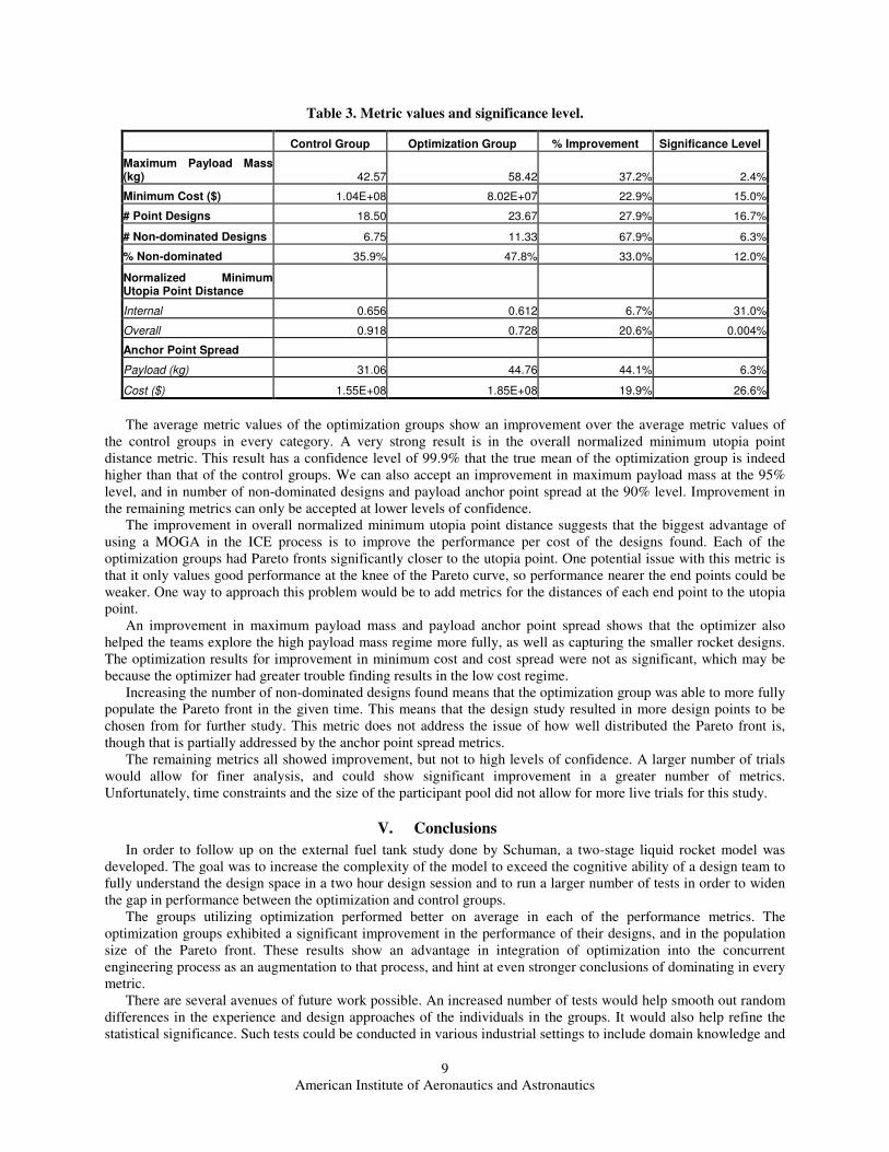
Table 3. Metric values and significance level.

Control Group Optimization Group % Improvement Significance Level

Maximum Payload Mass (kg) 42.57 58.42 37.2% 2.4%

Minimum Cost ($) 1.04E+08 8.02E+07 22.9% 15.0%

# Point Designs 18.50 23.67 27.9% 16.7%

# Non-dominated Designs 6.75 11.33 67.9% 6.3%

% Non-dominated 35.9% 47.8% 33.0% 12.0%

Normalized Minimum Utopia Point Distance

Internal 0.656 0.612 6.7% 31.0%

Overall 0.918 0.728 20.6% 0.004%

Anchor Point Spread

Payload (kg) 31.06 44.76 44.1% 6.3%

Cost ($) 1.55E+08 1.85E+08 19.9% 26.6%

The average metric values of the optimization groups show an improvement over the average metric values of

the control groups in every category. A very strong result is in the overall normalized minimum utopia point distance metric. This result has a confidence level of 99.9% that the true mean of the optimization group is indeed higher than that of the control groups. We can also accept an improvement in maximum payload mass at the 95% level, and in number of non-dominated designs and payload anchor point spread at the 90% level. Improvement in the remaining metrics can only be accepted at lower levels of confidence.

The improvement in overall normalized minimum utopia point distance suggests that the biggest advantage of using a MOGA in the ICE process is to improve the performance per cost of the designs found. Each of the optimization groups had Pareto fronts significantly closer to the utopia point. One potential issue with this metric is that it only values good performance at the knee of the Pareto curve, so performance nearer the end points could be weaker. One way to approach this problem would be to add metrics for the distances of each end point to the utopia point.

An improvement in maximum payload mass and payload anchor point spread shows that the optimizer also helped the teams explore the high payload mass regime more fully, as well as capturing the smaller rocket designs. The optimization results for improvement in minimum cost and cost spread were not as significant, which may be because the optimizer had greater trouble finding results in the low cost regime.

Increasing the number of non-dominated designs found means that the optimization group was able to more fully populate the Pareto front in the given time. This means that the design study resulted in more design points to be chosen from for further study. This metric does not address the issue of how well distributed the Pareto front is, though that is partially addressed by the anchor point spread metrics.

The remaining metrics all showed improvement, but not to high levels of confidence. A larger number of trials would allow for finer analysis, and could show significant improvement in a greater number of metrics. Unfortunately, time constraints and the size of the participant pool did not allow for more live trials for this study.

V. Conclusions

In order to follow up on the external fuel tank study done by Schuman, a two-stage liquid rocket model was developed. The goal was to increase the complexity of the model to exceed the cognitive ability of a design team to fully understand the design space in a two hour design session and to run a larger number of tests in order to widen the gap in performance between the optimization and control groups.

The groups utilizing optimization performed better on average in each of the performance metrics. The optimization groups exhibited a significant improvement in the performance of their designs, and in the population size of the Pareto front. These results show an advantage in integration of optimization into the concurrent engineering process as an augmentation to that process, and hint at even stronger conclusions of dominating in every metric.

There are several avenues of future work possible. An increased number of tests would help smooth out random differences in the experience and design approaches of the individuals in the groups. It would also help refine the statistical significance. Such tests could be conducted in various industrial settings to include domain knowledge and


10

experience level of the participants as control variables. Reexamining the metrics used is also important, as the metrics were the basis of the quantitative comparisons of the two design methods. In particular a metric to describe how well distributed (i.e. not clustered) the Pareto front points are would be useful. The rocket model, though adequate and benchmarked against the Delta family of launch vehicles, could be improved. Making it more physically accurate would make the results of the design session more representative of actual design work. Finally the MOGA used could be refined, since it took long periods of computation, and the points it found were somewhat off the local maxima. Improving the optimizer would benefit the optimization teams, which would strengthen the conclusions of this study.

Acknowledgments

Brian Bairstow was supported through a NDSEG graduate fellowship.

References 1Sobieszczanski-Sobieski, J., Haftka, R.T., “Multidisciplinary Aerospace Optimization: Survey of Recent Developments,”

Structural Optimization J., Vol. 14, No. 1, August 1997 2Schuman, T., “Integration of System-Level Optimization With Concurrent Engineering Using Parametric Subsystem

Modeling,” Master’s Thesis, Aeronautics and Astronautics Dept., Massachusetts Institute of Technology, Cambridge, MA, 2004. 3Schuman T., de Weck O.L., Sobieszczanski-Sobieski J., “Integrated System-level Optimization for Concurrent Engineering

with Parametric Subsystem Modeling”, AIAA-2005-2199, 1st AIAA Multidisciplinary Design Optimization Specialist Conference, Austin, Texas, April 18-21, 2005

4Bairstow, B., de Weck, O.L., Sobieszczanski-Sobieski, J., “Multiobjective Optimization of Two-Stage Rockets for Earth-To-Orbit Launch,” 2nd AIAA MDO Specialist Conference, May 2006.

5Miller, G. A., “The Magical Number Seven, Plus or Minus Two: Some Limits on Our Capacity for Processing Information,” The Psychological Review, Vol. 63, 1956, pp. 81-97.

6Cohanim, B. E., Hewitt, J. N., de Weck, O.L., “The Design of Radio Telescope Array Configurations using Multiobjective Optimization: Imaging Performance versus Cable Length,” The Astrophysical Journal Supplement Series, Vol. 154, October 2004, pp. 705-719.

7Ahuja, R. K., Orlin, J. B., Tiwari, A., “A Greedy Genetic Algorithm for the Quadratic Assignment Problem,” Computers

and Operations Research, Vol. 27, 2000, pp. 917-934. 8Parkin, K., Sercel, J., Liu, M., and Thunnissen, D., “ICEMaker: An Excel-Based Environment for Collaborative Design,”

2003 IEEE Aerospace Conference Proceedings, Big Sky, Montana, March 2003. 9Ross, S. M., Introduction to Probability and Statistics for Engineers and Scientists, 2nd ed., Academic Press, San Diego, CA,

2000, pp. 291-299.

[american institute of aeronautics and astronautics 48th aiaa/asme/asce/ahs/asc structures,...

Documents