AMERICAN ASSOCIATION OF WINE ECONOMISTS

AAWE WORKING PAPER No. 202

Economics

MACROECONOMIC DETERMINANTS OF WINE PRICES

Linda Jiao

Aug 2016

www.wine-economics.org

AAWEWorkingPapersarecirculatedfordiscussionandcommentpurposes.Theyhavenotbeensubjecttoapeerreviewprocess.Theviewsexpressedhereinarethoseoftheauthor(s)anddonotnecessarilyreflecttheviewsoftheAmericanAssociationofWineEconomistsAAWE.

©2016bytheauthor(s).Allrightsreserved.Shortsectionsoftext,nottoexceedtwoparagraphs,maybequotedwithoutexplicitpermissionprovidedthatfullcredit,including©notice,isgiventothesource.

1

Macroeconomic determinants of wine prices

Linda Jiao

Larefi – University of Bordeaux

Bordeaux Wine Economics

linda.jiao@u-bordeaux.fr

Abstract

This paper identifies the macroeconomic determinants of fine wine prices and estimates their

impacts on a monthly database from 1996 to 2015. The fine wine demand from emerging

markets plays a key role in fine wine pricing, and more precisely, on the fluctuation of Bordeaux

fine wine prices. Furthermore, the continuous weakening of the U.S. Dollar in real term favors

the fine wine prices to increase. Since 2011, the slowdown of economic growth in emerging

markets, followed by the depreciation of national currencies has engendered negative effects on

the fine wine market. Along with the process of financialization in the fine wine market, fine

wine prices have become more volatile. Factors such as money supply, real interest rate and the

growth of investment funds start to show their influence on fine wine pricing.

Keywords: wine, price, macroeconomics, emerging markets, financialization

JEL classification codes: C22 C26 Q11

2

1. Introduction

In the wine economic literature, many successful studies exist in the evolution of wine prices are

taken in the perspective of supply. The empirical analyses are mainly based on the hedonic price

approach to estimate the impact of each wine characteristic on the price determination

(Ashenfelter, 2008; Lecocq and Visser, 2006; Cardebat and Figuet, 2004).

Since Krasker (1979), the returns and the portfolio diversification benefits of fine wines have

been progressively studied by using auction prices and Liv-ex indices, the results mainly

confirmed the interest of fine wines started to become an attractive alternative financial asset.

With the financialization in the fine wine market, few researchers started to explore the linkage

between financial markets and wine markets, and discover the impact of macroeconomic factors

on wine price determination.

Fine wine price is sensitively related to economic dynamics. Since the first half of 2000s, fine

wine prices skyrocketed thanks to the growth of demand from emerging markets. In 2008, the

growth came to a sudden end on the eve of the financial crisis. Then the prices started to

fluctuate following the recession and the recovery of the economy. After the pick at 2011, fine

wine prices have been undergoing a continuous decline. This decline can be mainly explained by

the drop in demand: the slowdown of economic growth of emerging economies, the weakness of

the national currencies of certain emerging countries, and other unpredictable factors such as the

anti-corruption/gift-giving crackdown in China.

The establishment of the London International Vinters Exchange (Liv-ex) and the emergence of

wine investment funds accelerated the pace of financialization of the fine wine market. The wine

investment creates another type of demand in addition to the wine consumption. A prosperous

financial environment associated with low interest rates favors the fine wine investment. On the

other hand, fine wine prices have become more volatile following the up-and-down of economic

cycles.

Through existing literatures and evidences, the main idea of our research is developed as

illustrated in figure 1: macroeconomic factors can influence wine markets directly and indirectly.

When macroeconomic fluctuations take place, financial markets react immediately. And their

reactions will have impacts on wine markets (preferable fine wines) via the canals such as wealth

3

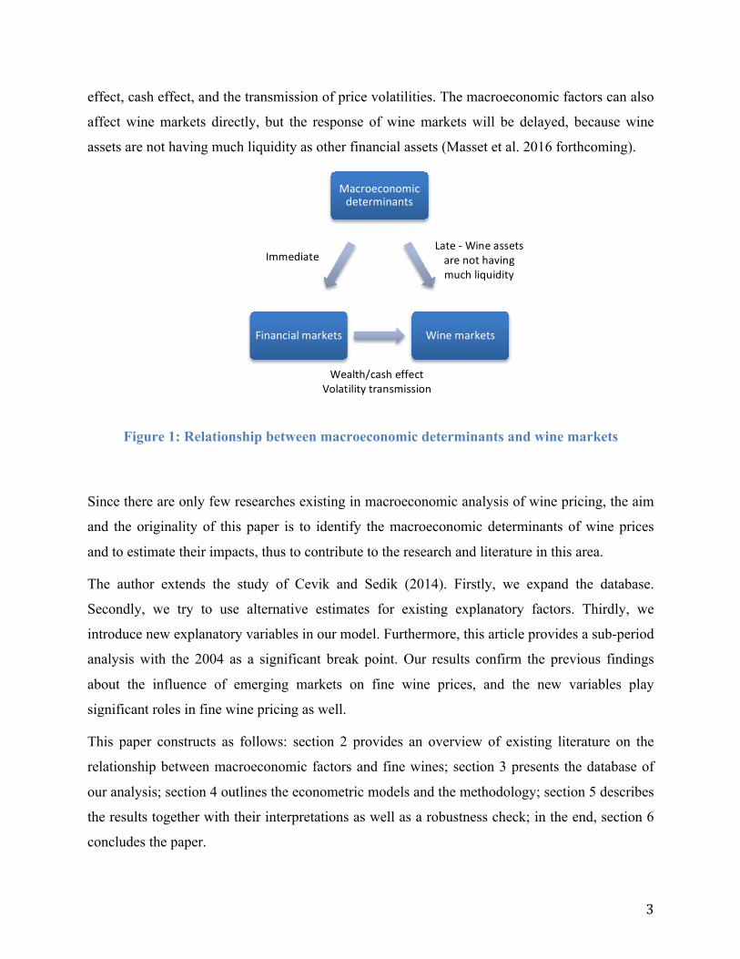
effect, cash effect, and the transmission of price volatilities. The macroeconomic factors can also

affect wine markets directly, but the response of wine markets will be delayed, because wine

assets are not having much liquidity as other financial assets (Masset et al. 2016 forthcoming).

Figure 1: Relationship between macroeconomic determinants and wine markets

Since there are only few researches existing in macroeconomic analysis of wine pricing, the aim

and the originality of this paper is to identify the macroeconomic determinants of wine prices

and to estimate their impacts, thus to contribute to the research and literature in this area.

The author extends the study of Cevik and Sedik (2014). Firstly, we expand the database.

Secondly, we try to use alternative estimates for existing explanatory factors. Thirdly, we

introduce new explanatory variables in our model. Furthermore, this article provides a sub-period

analysis with the 2004 as a significant break point. Our results confirm the previous findings

about the influence of emerging markets on fine wine prices, and the new variables play

significant roles in fine wine pricing as well.

This paper constructs as follows: section 2 provides an overview of existing literature on the

relationship between macroeconomic factors and fine wines; section 3 presents the database of

our analysis; section 4 outlines the econometric models and the methodology; section 5 describes

the results together with their interpretations as well as a robustness check; in the end, section 6

concludes the paper.

Macroeconomicdeterminants

Financialmarkets Winemarkets

Wealth/casheffect Volatilitytransmission

Immediate Late-Wineassetsarenothavingmuchliquidity

4

2. Fine wine price and macroeconomic factors

Wine literature has contributed a lot on analyzing wine price determination through hedonic

price approach, estimating the return, the performance and the portfolio diversification benefits

of wine investment. However, few papers have been devoted to discovering the influence of

macroeconomic and/or financial factors of wine prices.

Anderson K. et al. (2001) modeled and forecasted the world wine market based on household

income, population, and taste trends on the demand side along with the wine production factors

on the supply side under the background of wine industry globalization. Cevik and Sedik (2014)

pointed that, under the influences of common macroeconomic factors, fine wines seemed to

behave not differently from commodities. They modeled fine wine prices with the same

macroeconomic variables as crude oil prices, and their results confirmed the role of

macroeconomic determinants in fine wine price modeling. While on the demand side, they

analyzed separately the demand impacts of developed economies and emerging economies, also

the effects of world monetary developments. They included global wine production in their

model as a variable from the supply side. Results showed that the growth of demand from

emerging economies, supports fine wine prices, and the abundant global liquidity associated with

low interest rates seemed to amplify the space of price increase. As to the supply side, the effect

of wine production was limited.

Other factors can be also taken into account of wine price modeling. Literature indicates that the

real effective exchange rate influences commodity prices through the effect of demand (Reinhart

and Borensztein, 1994). For dollar-priced tradable goods, a decline in the value of dollar in real

term can raise the purchasing power of foreign consumers in real term, then the demand can be

expanded and the price will be lifted.

It can also find the impact of exchange rate on the wine market in literature. Lindsay P.J. (1987)

analyzed the effects of exchange rate and trade barriers on U.S. wine imports and exports.

Anderson and Wittwer (2013) included bilateral real exchange rates and the growth in China’s

import demand in global wine market modeling.

Since fine wine has been integrated into portfolio as an alternative financial asset, apart from the

indicator of money supply, the interest rate is another important monetary factor. In theory, the

real interest rate negatively affects the price of financial assets through the discount factor: a

5

lower interest rate in real term drops the discount factor, raises the present value of expected

future return and therefore the current price will be elevated. The behaviors of speculation may

accentuate the price volatility in the short-term when they are associated with weaker real

interest rates. Besides, low interest rate may encourage investors investing in equities or

alternative assets with higher returns; therefore they would raise their prices through demand.

Studies exist in this area for stock markets (e.g., FAMA and Schwert (1977), FAMA (1981) and

Christie (1982)) or commodity markets (e.g., Frankel (1986, 2008) and Beck (1993)). To our

knowledge, there still no such studies in the area of fine wine prices for now.

The fine wine investment fund has emerged since the end of 1990s1 as a result of the steady

return in fine wine and the need of portfolio diversification for investors, thereafter, wine

investment has been accepted as a valuable alternative financial asset by investors. The

emergence of private or institutional wine investment funds, along with the establishment of Liv-

ex accelerated the process of financialization of the fine wine market. The wine investment

creates a supplementary demand in addition to the wine consumption, such as the speculation of

the outstanding vintages of Bordeaux First Growth. The fine wine price is more volatile due to

the up-and-down of investment, which is affected by the volatilities of other financial assets

under the influence of the economic cycles. Faye et al. (2015) showed short-term causalities

between several fine wine auction prices and the MSCI World index; Cardebat and Jiao (2016

forthcoming) demonstrated the cointegration relationships of Liv-ex fine wine price indices with

certain stock market indices from the world level to specific countries, as well as the causalities

from stock markets to fine wine markets. Thus, a financial factor - financial asset of investment

funds as percentage of GDP - may be a useful explanatory variable for fine wine prices. This

indicator is considered as a measurement of financialization, which represents the evolution of

capital invested in financial assets and reflects the volatility in financial market along with the

economic cycles.

Aside from financial crisis, several additional unpredictable factors can affect wine prices.

Evidences showed that the political elements could not be ignored. The announcement of a new

policy may modify the condition of supply or demand (taking the negative impact of Chinese

government gift-giving crackdown for instance). Other random variables include technology

1 Ascot Wine Management Fine Wine Fund (Bahamas) is founded in 1999 ; Orange Wine Fund (Amsterdam) in 2001 ; Wine Investment Fund (UK) in 2003 ; Vintage Wine Fund (UK) in 2003 (no defunct)

6

progress in wine production or the changes in wine production surfaces, together with other

unpredictable factors in supply side such as weather conditions; they can all be captured by the

production. All these factors related to a supply or demand shock can be seized by dummy

variables in our model.

3. Data

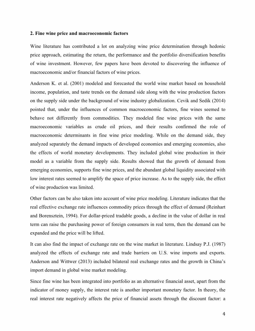
The database covers a timeframe from 1996 to 2015 in monthly frequency and consists of Liv-ex

Fine Wine Investables index (and Liv-ex Fine Wine 1000 index in the robustness check) as the

fine wine price, and explanatory variables on both supply side and demand side. The length of

the database allows us to capture information on different steps of the development of the fine

wine market along with the macroeconomic fluctuations during the last twenty years. Also, it is

based on the need of the availability of data for all concerned variables2.

Figure 2: Liv-ex Fine Wine Investables Index (Source: Liv-ex)

Liv-ex provides a global platform for fine wine traders. Professionals often consider their price

indices as a benchmark of fine wine exchange. Liv-ex Fine Wine Investables index started from

1988, and is one of their leading fine wine price indices, composed of most dominant

2 The Source of all macroeconomic data is from the OECD Statistics.

050

100150200250300350400

Jan-

96Se

p-96

May

-97

Jan-

98Se

p-98

May

-99

Jan-

00Se

p-00

May

-01

Jan-

02Se

p-02

May

-03

Jan-

04Se

p-04

May

-05

Jan-

06Se

p-06

May

-07

Jan-

08Se

p-08

May

-09

Jan-

10Se

p-10

May

-11

Jan-

12Se

p-12

May

-13

Jan-

14Se

p-14

May

-15

Liv-ex Fine Wine Investables Index

Liv-ex Fine Wine Investables Index

7

investment-grade wines. It contains around 200 Bordeaux red wines from 24 top chateaux dated

back to the 1982 vintage and chose on the basis of their Robert Parker rating scores. This index

is price weighted and calculated by the Liv-ex Mid Price method (the midpoint between the

current highest bid and lowest offer price) for each component wine with taking into account of

its scarcity3 . We also include Liv-ex Fine Wine 1000 index to enrich our analysis in the

robustness check section. The indices are sterling-based monthly price series. We convert it to a

dollar-based price series with historical monthly average sterling-dollar exchange rates and then

deflate it to real term with the U.S. consumer price index.

We take the global wine production as the variable from the supply side. The data is available in

the database of Organisation Internationale de la Vigne et du Vin (OIV). Since the wine grapes

harvest once a year, the production data is only available annually. For the demand side, we can

also find the annual global wine consumption in the database of the OIV. To construct monthly

data, we put the same production or consumption level for the twelve months of a given year in

our estimation.

In place of the Industrial Production Index in Cevik and Sedik (2014), we use the GDP as the

estimate of demand. It concerns two real-economy variables – the aggregated GDP of G-4

economies (the United States, the United Kingdom, the Euro Zone and Japan) and the aggregated

GDP of BRIC economies (Brazil, Russia, India and China). The G-4 economies can represent

both developed economies and “old” wine consuming countries, by contrary, the BRIC countries

represent emerging economies and “new” wine consuming countries. These two variables allow

us to estimate respectively the impact of developed and emerging economies on fine wine prices,

thus to distinguish the source of influence. The aggregated GDPs are weighted on the basis of the

size of each economy4. National GDPs expressed in national currencies are converted and

deflated into real dollar. Since GDPs are in quarterly frequency, all months have the same GDP

level for a given quarter in our estimation.

3 A coefficient of scarcity is applied to the vintages older than 15 years and Petrus and Ausone because of their small production. For more information concerning Liv-ex indices and their components, see https://www.liv-ex.com/. 4 On average for the entire period: in the aggregated GDP of G-4 economies, the U.S. represents 42.5%, the U.K. 7.2%, the Euro Zone 33.8% and Japan 16.5% ; in the aggregated GDP of BRIC economies, Brazil represents 20.8%, Russia 13.5%, India 15.5%, and China 50.2%.

8

Then we introduce the real effective exchange rate (REER) of U.S. Dollar to capture the effect of

real exchange rate on fine wine price, the data which is published monthly by the Bank of

International Settlement.

Normally, wine investment is a middle/long term engagement. For instance, wine investment

funds used to provide contracts for a minimum 5-year engagement. And by definition, the broad

money covers assets with less liquidity5. Thus, we choose the aggregated M3 of G-4 economies

instead of the excess liquidity (the difference between the changes in M2 and the long term

potential growth rate and velocity) in Cevik and Sedik (2014), to estimate the impact of global

monetary development on fine wine prices. The aggregated M3 of the G-4 is in monthly

frequency, weighted by GDPs and expressed in real dollar.

Another monetary variable is the U.S. real interest rates. According to the Fisher equation, the

real interest rate is calculated approximately from the nominal interest rate minus the inflation

rate.

As mentioned before, we use the financial assets of investment funds as percentage of GDP in

the U.S. to estimate the impact of financialization on fine wine prices. This indicator is

calculated from the sum of U.S. households and institutions’ financial assets of investment funds

divided by the U.S. GDP.

We put time dummy variables to capture all other elements which can conduct production or

demand shocks (such as the financial crisis or the Chinese government gift-giving crackdown),

and extraordinary or appalling vintage. If an event or several events happen in a specific year, all

months equal to 1 for this year, and all the other time spots equal to 0. For example, DM2008

represents all the twelve months of 2008 equal to 1 and the others equal to 0.

4. Methodology

The logarithms of the data series are used in further econometric estimations. To Deal with the

seasonality of certain variables (GDPs and M3), we use X12 seasonality adjustment tool to

smooth the data. We apply Augmented Dickey-Fuller unit root test to test the stationarity of data

series in level or in difference. According to the tests, the series of global wine production and

5 “Broad money is the sum of M2, repurchase agreements, money market fund shares/units and debt securities up to two years.” Source OECD.

9

aggregated M3 of the G-4 are stationary in level, and other variables are integrated of the first

order. In further regressions, all variables are stationary; we include the wine production and M3-

G4 in level and other variables in difference. For the aggregated GDPs and the global wine

consumption, we use respectively three-month and twelve-month differences instead of first

differences. Detailed results of ADF test are presented in annex 1.

Variables will be estimated in two econometric models to avoid the potential correlation problem

among explanatory variables.

- Model 1(with aggregated M3 of G-4 economies):

∆𝑷𝒕 = 𝜷𝟎 +𝜷𝟏∆𝑮𝑫𝑷𝑮𝟒,𝒕 +𝜷𝟐∆𝑮𝑫𝑷𝑩𝑹𝑰𝑪,𝒕 + 𝜷𝟑𝑷𝑹𝑶𝑫𝒕 +𝜷𝟒∆𝑪𝑶𝑵𝑺𝒕 + 𝜷𝟓∆𝑹𝑬𝑬𝑹𝒕 +

𝜷𝟔𝑴𝟑𝑮𝟒𝒕 + 𝜷𝟕𝑫𝑴+ 𝜺𝒕

- Model 2 (with U.S. real interest rate and U.S. investment funds as percentage of GDP):

∆𝑷𝒕 = 𝜷𝟎 +𝜷𝟏∆𝑮𝑫𝑷𝑮𝟒,𝒕 +𝜷𝟐∆𝑮𝑫𝑷𝑩𝑹𝑰𝑪,𝒕 + 𝜷𝟑𝑷𝑹𝑶𝑫𝒕 +𝜷𝟒∆𝑪𝑶𝑵𝑺𝒕 + 𝜷𝟓∆𝑹𝑬𝑬𝑹𝒕 +

𝜷𝟔∆𝑰𝑹𝒕 + 𝜷𝟕∆𝑰𝑭𝒕 + 𝜷𝟕𝑫𝑴+ 𝜺𝒕

where ∆𝑷𝒕 is the growth rate of real fine wine price calculated from Liv-ex Fine Wine

Investables or Liv-ex Fine Wine 1000 (in robustness check); ∆𝑮𝑫𝑷𝑮𝟒,𝒕 is the growth rate of

aggregated GDP of G-4 economies; ∆𝑮𝑫𝑷𝑩𝑹𝑰𝑪,𝒕 is the growth rate of aggregated GDP of BRIC

economies; 𝑷𝑹𝑶𝑫𝒕 is the global wine production; ∆𝑪𝑶𝑵𝑺𝒕is the growth rate of global wine

consumption. ∆𝑹𝑬𝑬𝑹𝒕 is the growth rate of real effective exchange rate of the US Dollar;

𝑴𝟑𝑮𝟒𝒕 is the aggregated money supply of G-4 economies; ∆𝑰𝑹𝒕 is the growth rate of the U.S.

real interest rate; ∆𝑰𝑭𝒕 is the growth rate of financial assets of investment funds as percentage of

GDP in the U.S.; 𝑫𝑴s are the time dummy variables; 𝛽s are the parameters to be estimated and

𝜀@ is the error term.

Firstly, we use the Ordinary Least Squares Method to estimate the equations. Followed by the

suggestion of Cevik and Sedik (2014)6, we also apply the Generalized Method of Moments to

correct the potential endogeneity problem of explanatory variables. We use J-statistic as a test of

over-identifying moment conditions. According to our statistics, the null hypothesis that the 6 They indicate that some explanatory variables may be correlated with the error term, because the fluctuation of wine price could have impacts on its production and demand, and also the explanatory variables may be measured with error. So, they suggested using GMM to avoid above potential problems.

10

over-identifying restrictions are satisfied cannot be rejected. In the presence of residual

heteroscedaticity and autocorrelation, the Newey-West estimator is used to address this problem.

5. Empirical results and interpretation

Table 1 and 2 show the results of our first model on the full time period and the sub-period, and

Table 3 and 4 present the results of the second model (to compare with the results of Cevik and

Sedik (2014), see annex 2).

Table 1: Results for Model 1 without time dummy variables

Equation 1 Equation 2 Equation 3 Equation 4

1996 - 2015 1996 -2015 2004 - 2015 2004 - 2015

LS GMM LS GMM

Variable Coef. t-Stat. Coef. t-Stat. Coef. t-Stat. Coef. t-Stat.

GDP G4 -0.04 -0.35 -0.22 -2.01** -0.05 -0.33 -0.02 -0.22

GDP

BRIC 0.23 2.22** 0.17 2.29** 0.34 2.24** 0.26 2.63**

PROD 0.07 1.22 0.03 0.55 0.07 1.01 0.06 0.99

CONS 0.18 1.09 0.24 1.78* 0.41 2.08** 0.40 3.61***

REER -1.22 -6.45*** -1.73 -7.02*** -1.36 -6.49*** -1.61 -7.09***

M3G4 -0.02 -0.96 -0.01 -0.48 0.06 1.42 0.07 2.41**

C -0.33 -1.02 -0.12 -0.44 -0.68 -1.29 -0.62 -1.50

Adjusted

R2 0.34 0.32 0.48 0.47

Num. Obs. 231 227 141 141

Breakpoint Test: 2004m01 t-Stat. Prob.

Andrews-Fair Wald Stat.7 18.00 0.01

Hall and Sen O Stat.8 29.73 0.76

* p < 0.1, ** p < 0.05, *** p < 0.01.

7 H0 : there are no structural breaks in the equation parameters. 8 H0 : the over-identifying restrictions are stable over the entire sample.

11

Table 2: Results for Model 1 with time dummy variables

Equation 5 Equation 6 Equation 7 Equation 8

1996 - 2015 1996 -2015 2004 - 2015 2004 - 2015

LS GMM LS GMM

Variable Coef. t-Stat. Coef. t-Stat. Coef. t-Stat. Coef. t-Stat.

GDP G4 -0,07 -0,56 -0,18 -1,65 -0,09 -0,67 -0,07 -0,60

GDP

BRIC 0,22 2,33** 0,18 2,29** 0,31 2,53** 0,27 3,39***

PROD 0,02 0,33 -0,03 -0,58 0,01 0,19 -0,01 -0,16

CONS -0,10 -0,53 -0,14 -0,84 0,14 0,47 0,28 1,15

REER -1,22 -7,20*** -1,75 -7,10*** -1,34 -7,15*** -1,51 -6,79***

M3G4 -0,01 -0,42 0,00 -0,06 0,04 1,15 0,05 2,04**

DM1997 0,02 2,46** 0,02 3,82***

DM2006 0,03 2,24** 0,03 2,41** 0,02 1,22 0,02 1,21

DM2008 -0,04 -2,38** -0,04 -3,03*** -0,03 -2,16** -0,03 -3,18***

DM2010 0,01 2,15** 0,01 1,93* 0,01 1,45 0,01 2,07**

DM2011 -0,01 -1,34 -0,02 -1,71* -0,02 -1,59 -0,02 -2,52**

C -0,07 -0,23 0,15 0,60 -0,25 -0,49 -0,16 -0,37

Adjusted

R2 0.44 0.41 0.56 0.55

Num. Obs. 231 227 141 141

* p < 0.1, ** p < 0.05, *** p < 0.01.

We consider 2004 as a time point where the financialization of the fine wine market activated,

thus a breakpoint in our estimation. The reasons are as follows: firstly, through the figure, we can

observe directly that the significant evolution of fine wine prices started from 2004, before this

date, the index was flat except during the period of the Asian financial crisis; secondly, the

majority of Liv-ex fine wine indices started from December 2003 and all indices were based or

rebased at 100 in December 2003; thirdly, several Large and credible wine investment funds

have been established in the U.K. since 2003. In addition, the Andrews-Fair Wald and Hall and

12

Sen Statistics confirm that January 2004 is a significant breakpoint over the entire sample9. The

variables suit better on the period of 2004-2015 than on the full time period, with an

improvement of 0.15 for the adjusted R2 on average.

The global wine consumption and the aggregated GDP of the BRICs have significant positive

signs. By contrary, the global wine production and the aggregated GDP of G-4 economies are

not statistically significant 10 . This may indicate that during the relevant time period, the

fluctuation of fine wine price is mainly driven by the demand side, and more precisely, driven by

the demand from emerging markets. However, the fine wine prices are not sensitive to the

production, or the global wine production may be not an appropriate factor to explain the price of

fine wine, as the volume of fine wine is negligible in the total volume of global production.

During the 2000s’, the increasing demand from emerging countries was a powerful factor that

has pushed the fine wine price to rise steeply. In response to the shock of the global financial

crisis, actions were taken by central banks, including China’s RMB 4 trillion stimulus package.

In the meanwhile, the popularity of fine wine among wealthy consumers from emerging

countries, have brought a strongly growing demand. The fine wine market quickly recovered

from the crisis and experienced a strong upward momentum. Since the middle of 2011, following

the chute in demand due to the slowdown of economic growth in emerging markets, the fine

wine market started to decline. Another responsible factor could be the gift-giving crackdown

policy of Chinese government. Besides, prestige-seeking consumers started to be rational against

the “red obsession”.

Statistically, the aggregated GDP of G-4 does not show any significant impact on fine wine

prices, but still, the G-4 economies are important markets for fine wines. Imagining if we could

remove the shock caused by the financial crisis, the demand from the developed countries – the

traditional wine consumption markets may be relatively less volatile on the entire time period.

For many prestige Bordeaux wine estates like the best-performing First Growth – Mouton

9 Andrews-Fair Wald and Hall and Sen tests are applied to the equation estimated by GMM. We also applied Chow Breakpoint test for the equation estimated by LS, the null hypothesis that no break at specified breakpoint is rejected. 10 The aggregated GDP of G-4 appears significant with a negative sign in equation 2, 10 and 14 estimated by GMM. It is a coincidence that can be only explained by the pure statistic movements. Besides, the variable is not significant in any other equation.

13

Rothschild, they trust La Place11 a lot and keep a strong market in Europe12. In the meanwhile,

the U.S. has been a growing market in fine wine as well. However, the price of top-end wines

skyrocketed due to the speculation on the secondary market where a considerable demand was

contributed by the consumers or investors from emerging countries.

The real effective exchange rate of U.S. Dollar appears with strong and highly significant

negative coefficients in every equation. The continuous weakening of the U.S. Dollar in real

term favored the purchasing power of consumers or collectors from emerging markets, which

encouraged further their wish of buying fine wines. The depreciation of national currencies

together with the slowdown of economic growth in emerging countries harmed their purchasing

power in real term, and therefore the demand declined and the price dropped.

The aggregated money supply of G-4 is not statistically significant on the full time period.

However, it performs significant and positive on the period of 2004 – 2015. The impact of

monetary factor appeared when the financialization of the fine wine market started. Along with

the process of financialization, fine wines have been more exposed to capital flows and more

sensitive to the economic cycles. The abundance of money supply, associated with low interest

rates, may favor the investment in fine wines, and as a result, increase the supplementary demand

in financial dimension. When investors are short of liquidity during the financial crisis, they can

cash the fine wine assets to reduce the difficulties.

11 La Place, La Place of Bordeaux, refers to the brokers and negociants in Bordeaux. 12 Source : Interview with Philippe Dhalluin of Mouton Rothschild by Liv-ex.

14

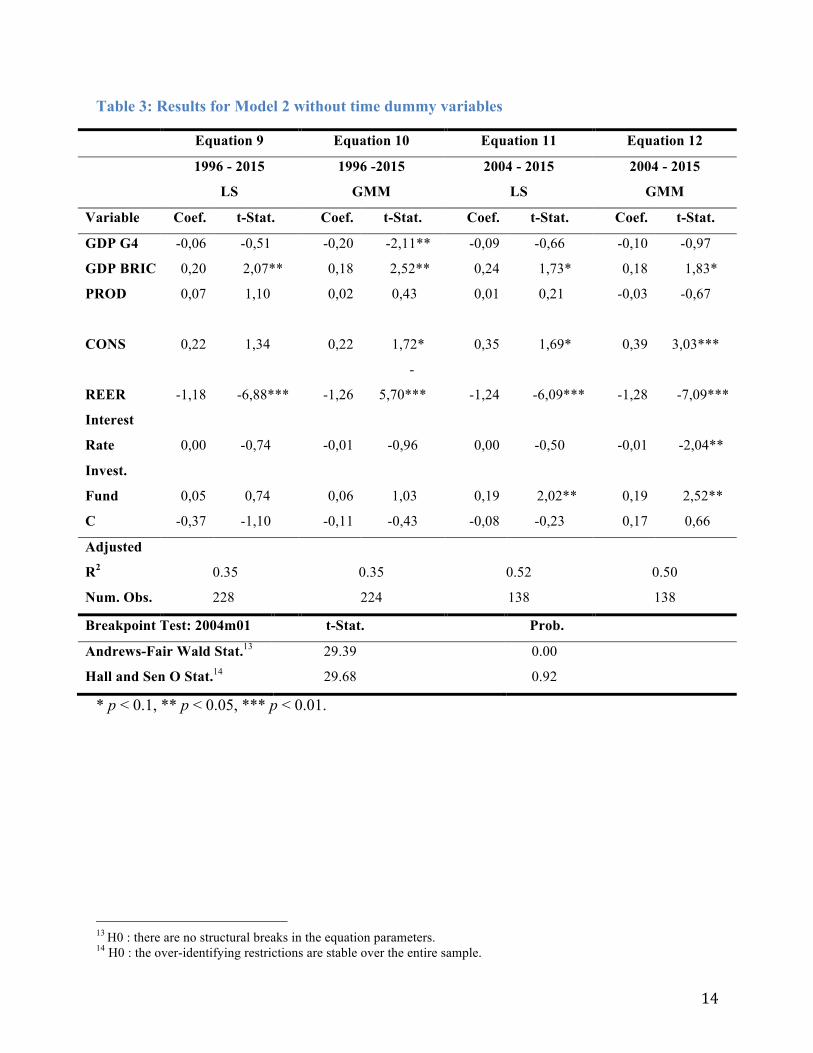
Table 3: Results for Model 2 without time dummy variables

Equation 9 Equation 10 Equation 11 Equation 12

1996 - 2015 1996 -2015 2004 - 2015 2004 - 2015

LS GMM LS GMM

Variable Coef. t-Stat. Coef. t-Stat. Coef. t-Stat. Coef. t-Stat.

GDP G4 -0,06 -0,51 -0,20 -2,11** -0,09 -0,66 -0,10 -0,97

GDP BRIC 0,20 2,07** 0,18 2,52** 0,24 1,73* 0,18 1,83*

PROD 0,07 1,10 0,02 0,43 0,01 0,21 -0,03 -0,67

CONS 0,22 1,34 0,22 1,72* 0,35 1,69* 0,39

3,03***

REER -1,18 -6,88*** -1,26

-

5,70*** -1,24 -6,09*** -1,28 -7,09***

Interest

Rate 0,00 -0,74 -0,01 -0,96 0,00 -0,50 -0,01 -2,04**

Invest.

Fund 0,05 0,74 0,06 1,03 0,19 2,02** 0,19 2,52**

C -0,37 -1,10 -0,11 -0,43 -0,08 -0,23 0,17 0,66

Adjusted

R2 0.35 0.35 0.52 0.50

Num. Obs. 228 224 138 138

Breakpoint Test: 2004m01 t-Stat. Prob.

Andrews-Fair Wald Stat.13 29.39 0.00

Hall and Sen O Stat.14 29.68 0.92

* p < 0.1, ** p < 0.05, *** p < 0.01.

13 H0 : there are no structural breaks in the equation parameters. 14 H0 : the over-identifying restrictions are stable over the entire sample.

15

Table 4: Results for Model 2 with time dummy variables

Equation 13 Equation 14 Equation 15 Equation 16

1996 - 2015 1996 -2015 2004 - 2015 2004 - 2015

LS GMM LS GMM

Variable Coef. t-Stat. Coef. t-Stat. Coef. t-Stat. Coef. t-Stat.

GDP G4 -0,09 -0,79 -0,21 -2,01** -0,14 -0,97 -0,10 -1,07

GDP BRIC 0,22 2,27** 0,23 2,83** 0,23 2,05** 0,21 2,55**

PROD 0,02 0,39 -0,01 -0,15 0,00 -0,05 -0,06 -1,22

CONS -0,09 -0,47 -0,12 -0,73 0,12 0,40 0,23 1,14

REER -1,24 -7,71*** -1,63 -7,17*** -1,27 -6,89*** -1,43 -7,52***

Interest

Rate -0,01 -1,31 -0,01 -1,16 -0,01 -1,00 -0,01 -1,95*

Invest.

Fund -0,03 -0,59 -0,06 -1,21 0,10 1,17 0,06 0,72

DM1997 0,02 2,77** 0,02 3,30***

DM2006 0,03 2,34** 0,03 2,32** 0,02 1,27 0,01 1,26

DM2008 -0,04 -2,56** -0,04 -3,45*** -0,03 -1,73* -0,03 -3,36***

DM2010 0,01 2,41** 0,01 2,37** 0,02 1,98** 0,01 1,93*

DM2011 -0,02 -1,62 -0,02 -2,39** -0,01 -1,31 -0,02 -3,04***

C -0,11 -0,39 0,04 0,15 0,02 0,04 0,32 1,21

Adjusted

R2 0.45 0.43 0.58 0.56

Num. Obs. 228 224 138 138

* p < 0.1, ** p < 0.05, *** p < 0.01.

Table 3 and 4 confirm the previous results of model 1. In addition, the U.S. real interest rate15

and the U.S. investment fund as percentage of GDP appear significant on the period of 2004 -

2015. The influence of real interest rate is not very robust, since it only has a weak negative

coefficient of 0.01 at the 10% significance, and only in the GMM equations. The growth of the

investment fund has a clearer positive impact on fine wine prices, which confirms the

financialization has played an important role in the fine wine market since 2004. We also

15 Here, it presents the results of the U.S. short-term real interest rate. The author also tries the long-term real interest rate, but it appears less significant. Additional results are available on request.

16

estimate the impact of the investment fund with the first model: create a combination of the

investment fund and the development of the money supply. We obtain positive and significant

coefficients for the investment fund as well16. However, when we add dummy variables in the

equations, the influence of investment fund – the supplementary demand in fine wine seems to

be absorbed by the dummies.

The introduction of dummy variables improves the adjusted R2. In Table 2 and 4, we list the time

dummy variables that appear significant. The dummy variables absorb the shocks from the

consumption, so the global consumption is not significant any more in the equations with

dummies. The results also confirm the negative influence due to the Subprime crisis in 2008,

China-led boom during 2009-2010 and the market depression followed by the slowdown of

economic growth in emerging markets since 2011.

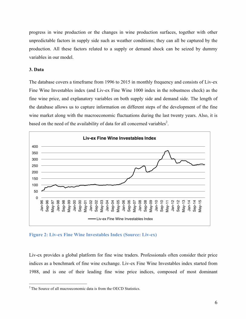
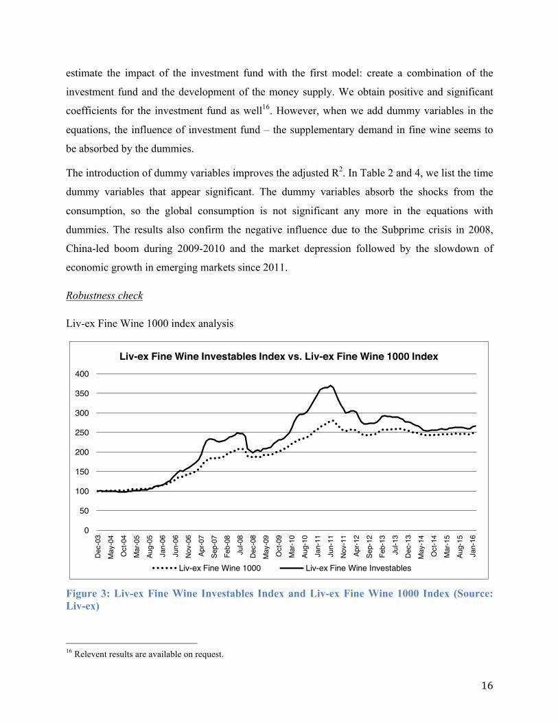
Robustness check

Liv-ex Fine Wine 1000 index analysis

Figure 3: Liv-ex Fine Wine Investables Index and Liv-ex Fine Wine 1000 Index (Source: Liv-ex)

16 Relevent results are available on request.

0

50

100

150

200

250

300

350

400

Dec

-03

May

-04

Oct

-04

Mar

-05

Aug-

05Ja

n-06

Jun-

06N

ov-0

6Ap

r-07

Sep-

07Fe

b-08

Jul-0

8D

ec-0

8M

ay-0

9O

ct-0

9M

ar-1

0Au

g-10

Jan-

11Ju

n-11

Nov

-11

Apr-1

2Se

p-12

Feb-

13Ju

l-13

Dec

-13

May

-14

Oct

-14

Mar

-15

Aug-

15Ja

n-16

Liv-ex Fine Wine Investables Index vs. Liv-ex Fine Wine 1000 Index

Liv-ex Fine Wine 1000 Liv-ex Fine Wine Investables

17

According to Liv-ex, Bordeaux region dominants the fine wine market, and represents nearly

80% of the total trade by value. Liv-ex Fine Wine Investables index is considered as one of the

most representative fine wine price indices. However, it is composed of only the most

financialized Bordeaux wines. Thus, to confirm the previous results, one needs to apply our

model to a fine wine price index that covers a wider range of wine regions - Liv-ex Fine Wine

1000 index. This index is price-weighted, including 7 sub-indices from six main regions:

Bordeaux 500, Bordeaux Legend 50, Burgundy 150, Champagne 50, Rhone 100, Italy 100, Rest

of the World 5017. Each sub-index represents the price movement of the ten most physical

vintages for the leading wines of the region, except for Bordeaux Legend 50 that includes only

50 top Bordeaux wines from exceptional elder vintages. The data of Liv-ex Fine Wine 1000 is

only available since December 2003. As we can see from the figure below, the composition of

other regions’ wines makes the Fine Wine 1000 index less volatile than Fine Wine Investables

index.

Table 5 and 6 show the results with Liv-ex Fine Wine 1000 index. These results confirm the

expecting impacts of macroeconomic variables on fine wine prices, but with less influence from

the emerging markets. The impact of BRIC economies is only significant in model 1 with

dummies. This finding coincides with the results of Cardebat and Jiao (2016 forthcoming) that

the linkages between emerging markets and fine wine markets are less significant when come to

the wines from other regions apart from Bordeaux. It might indicate that the major role of

emerging markets on Liv-ex Fine Wine Investables index is due to their high demand on prestige

Bordeaux wines, especially the First Growths, as to the wines from other regions, their influence

is limited. The real effective exchange rate of the U.S. dollar is highly significant in every

equation. However, the impact of aggregated money supply comes out with mixed results and

the real interest rate does not show any significant effect on Liv-ex Fine Wine 1000. In addition,

the results confirm the positive sign of the increase in investment funds on fine wine pricing.

17 Liv-ex Fine Wine 1000 Index is price weighted: Bordeaux 500 – 46%; Bordeaux Legends 50 – 22%; Burgundy 150 – 14%; Champagne 50 – 3%; Rhone 100 – 4%; Italy 100 – 7%; Rest of the World 50 – 4%. See https://www.liv-ex.com/ for more details concerning the component wines and vintages.

18

Table 5: Results for Liv-ex Fine Wine 1000 (model 1 and 2) without time dummy variables

Equation 17 Equation 18 Equation 19 Equation 20

2004 – 2015 2004 - 2015 2004 - 2015 2004 - 2015

LS GMM LS GMM

Variable Coef. t-Stat. Coef. t-Stat. Coef. t-Stat. Coef. t-Stat.

GDP G4 0,07 0,90 0,03 0,45 0,05 0,58 -0,04 -0,60

GDP BRIC 0,18 1,63 0,13 1,56 0,08 1,00 0,10 1,59

PROD 0,06 1,29 0,08 2,00** 0,02 0,50 0,03 0,67

CONS 0,30 2,31** 0,23 2,34** 0,26 2,06** 0,19 1,78*

REER -1,24 -7,38*** -1,64 -7,77*** -1,12 -6,92*** -1,25 -6,75***

M3G4 0,04 1,53 0,05 2,48**

Interest

Rate 0,00 -0,85 0,00 -0,74

Invest.

Fund 0,15 2,34** 0,17 3,69***

C -0,54 -1,53 -0,69 -2,45** -0,11 -0,50 -0,15 -0,68

Adjusted

R2 0.57 0.54 0.60 0.59

Num. Obs. 141 141 138 138

* p < 0.1, ** p < 0.05, *** p < 0.01.

19

Table 6: Results for Liv-ex Fine Wine 1000 (model 1 and 2) with time dummy variables

Equation 17 Equation 18 Equation 19 Equation 20

2004 – 2015 2004 - 2015 2004 - 2015 2004 - 2015

LS GMM LS GMM

Variable Coef. t-Stat. Coef. t-Stat. Coef. t-Stat. Coef. t-Stat.

GDP G4 0,04 0,48 0,02 0,21 0,02 0,23 -0,03 -0,39

GDP BRIC 0,16 1,93* 0,15 2,05** 0,09 1,13 0,11 1,55

PROD 0,02 0,51 0,01 0,30 0,01 0,25 -0,02 -0,57

CONS 0,11 0,57 0,25 1,39 0,11 0,59 0,19 1,35

REER -1,22 -8,44*** -1,47 -7,09*** -1,14 -8,09*** -1,34 -6,90***

M3G4 0,03 1,38 0,04 2,12**

Interest

Rate 0,00 -1,29 0,00 -0,81

Invest.

Fund 0,10 1,88* 0,09 1,73*

DM2006 0,01 1,38 0,00 0,47 0,01 1,38 0,01 0,91

DM2008 -0,02 -1,74* -0,01 -2,68** -0,01 -1,33 -0,01 -1,78*

DM2010 0,00 0,58 0,00 0,37 0,01 1,27 0,00 1,01

DM2011 -0,01 -1,16 -0,01 -1,91* 0,00 -0,71 -0,01 -1,54

C -0,26 -0,83 -0,24 -0,80 -0,06 -0,25 0,12 0,57

Adjusted

R2 0.61 0.59 0.62 0.61

Num. Obs. 141 141 138 138

* p < 0.1, ** p < 0.05, *** p < 0.01.

6. Conclusion

This paper empirically identified the macroeconomic determinants of fine wine prices and

estimated their impacts on a monthly database from 1996 to 2015. This time period allowed us to

capture information on different stages of the development of the fine wine market along with

the macroeconomic fluctuations during the last twenty years. And we chose 2004 as a breakpoint

where fine wines started to be more financialized and behave more sensitively to the economic

cycles.

20

Based on our results, the growth of fine wine demand from emerging markets seemed to play a

major role in fine wine price modeling, while the demand from developed markets did not appear

statistically significant. The continuous weakening of the U.S. Dollar in real term favored the

fine wine prices through the increasing of demand. Stronger national currencies encouraged the

buyers from emerging economies of purchasing fine wines. Since 2011, the slowdown of

economic growth in emerging markets followed by the depreciation of national currencies has

engendered negative effects on fine wine market. However, based on our results of the

robustness check, the strong influence of emerging markets seemed could only dominate the

price fluctuation of Bordeaux fine wines, due to their “red obsession” in Bordeaux First Growths.

As to the wines from other regions, the impact of emerging markets was very limited.

Along with the process of financialization in the fine wine market, the aggregated money supply,

the real interest rate and the financial assets of investment funds as percentage of GDP started to

show their influence on fine wine pricing. The real interest rate seemed to have a limited

negative impact. Nevertheless, the growth of money supply associated with lower interest rates

in real term did incite the investment in alternative financial assets including fine wines. The

wine investment, by private collectors or professional investment fund, created a supplementary

demand in addition to the wine consumption. As a result, the financial markets can influence fine

wine markets directly through wealth or cash effect. A prosperous financial environment could

favor the fine wine prices to increase; on the other hand, fine wine prices became more volatile

under unstable financial conditions.

In the author’s opinion, 2016 is a new start. For investors, the fine wine investment is better to be

a mid to long-term engagement; the drop of fine wine prices since 2011 does not only have its

negative side, because it hauls back the irrational growth to a long-term equilibrium. As for wine

professionals, facing the slowdown of economic growth in emerging markets, it is important to

rebalancing the market share among Europe, Asia, and the Americas.

Along with hedonic price modeling, our research can provide a complementary analysis in the

macroeconomic approach for wine price modeling and forecasting.

21

References

Akram, Q. F. (2009). Commodity prices, interest rates and the dollar. Energy economics, 31(6), 838-851. Anderson, K., Norman, D., & Wittwer, G. (2001). Globalization and the world’s wine markets: overview. Anderson, K., & Wittwer, G. (2013). Modeling global wine markets to 2018: Exchange rates, taste changes, and China’s import growth. Journal of Wine Economics, 8(02), 131-158. Ashenfelter, O. (2008). Predicting the quality and prices of Bordeaux wine. The Economic Journal, 118(529), F174-F184. Beck, S. E. (1993). A rational expectations model of time varying risk premia in commodities futures markets: theory and evidence. International Economic Review, 149-168. Borensztein, E., & Reinhart, C. M. (1994). The macroeconomic determinants of commodity prices. Staff Papers-International Monetary Fund, 236-261. Cardebat, J. M., & Figuet, J. M. (2004). What explains Bordeaux wine prices?. Applied Economics Letters, 11(5), 293-296. Cardebat, J.M., & JIAO, L. (Forthcoming 2016). The long-term financial drivers of fine wine prices: The role of emerging markets Cevik, S., & Saadi Sedik, T. (2014). A Barrel of Oil or a Bottle of Wine: How Do Global Growth Dynamics Affect Commodity Prices?. Journal of Wine Economics, 9(01), 34-50. Christie, A. A. (1982). The stochastic behavior of common stock variances: Value, leverage and interest rate effects. Journal of financial Economics, 10(4), 407-432. Fama, E. F. (1981). Stock returns, real activity, inflation, and money. The American Economic Review, 71(4), 545-565. Fama, E. F., & Schwert, G. W. (1977). Asset returns and inflation. Journal of financial economics, 5(2), 115-146. Frankel, J. A. (1986). Expectations and commodity price dynamics: The overshooting model. American Journal of Agricultural Economics, 68(2), 344-348. Faye, B., Le Fur, E., & Prat, S. (2015). Dynamics of fine wine and asset prices: evidence from short-and long-run co-movements. Applied Economics, 47(29), 3059-3077.

Frankel, J.A., 2008. The effect of monetary policy on real commodity prices. In Asset Prices and Monetary Policy. Ed. John Y. Campbell, NBER, University of Chicago, Chicago. And NBER Working Paper 12713. Krasker, W. S. (1979). The rate of return to storing wines. The Journal of Political Economy, 1363-1367. Lecocq, S., & Visser, M. (2006). What determines wine prices: Objective vs. sensory characteristics. Journal of Wine Economics, 1(01), 42-56.

22

Lindsay, P. J. (1987). An analysis of the effects of exchange rates and trade barriers on the US wine trade (Doctoral dissertation, PhD thesis, University of California at Davis, California).

Masset, P., Cardebat, J. M., Faye, B., & Le Fur, E. (Forthcoming 2016). Analyzing the risk of an illiquid asset – The case of fine wine

Annex 1: Unit Root Test – Augmented Dickey-Fuller Test

Series t-Stat. in Level t-Stat. in Difference Result

Liv-ex Fine Wine Investables -2.19 trend / cons** -9.94*** trend/cons I(1)

Liv-ex Fine Wine 1000 -1.82 trend / cons* -5.72*** trend/cons I(1)

GDP G4 0.45 trend/cons -7.26*** trend/cons I(1)

GDP BRIC -1.87 trend* / cons* -4.12*** trend/cons** I(1)

World wine production -3.42*** trend/cons*** I(0)

World wine consumption 0.74 trend/cons -2.95*** trend/cons I(1)

Real effective exchange rate $ 0.42 trend/cons -10.13*** trend/cons I(1)

M3 G4 -3.58** trend***/cons*** I(0)

Real interest rate US -1.56 trend / cons -7.32*** trend/cons I(1)

Investment fund in % of GDP US -2.72 trend**/cons*** -15.97*** trend/cons*** I(1)

***, **, * denotes rejection of null hypothesis (non-stationary for unit root test, non-significance for trend or constant) at 1% , 5%, and 10% significance level.

Annex 2: Results of Cevik and Sedik (2014)