amca publication 203 r2007
TRANSCRIPT
The International Authority on Air System Components
AIR MOVEMENT AND CONTROLASSOCIATION INTERNATIONAL, INC.
AMCAPublication 203-90
Field Performance Measurement of Fan Systems
(R2007)

AMCA PUBLICATION 203-90 (R2007)
Field Performance Measurement
of Fan Systems
Air Movement and Control Association International, Inc.
30 West University Drive
Arlington Heights, IL 60004-1893
© 2007 by Air Movement and Control Association International, Inc.
All rights reserved. Reproduction or translation of any part of this work beyond that permitted by Sections 107 and
108 of the United States Copyright Act without the permission of the copyright owner is unlawful. Requests for
permission or further information should be addressed to the Executive Director, Air Movement and Control
Association International, Inc. at 30 West University Drive, Arlington Heights, IL 60004-1893 U.S.A.
Forward
The original edition of Publication 203 was released in 1976. This, the second edition, updates much of theinformation that was presented.
Annex K (estimating the power output of three phase motors) and Annex L (estimating belt drive losses) wererewritten and adjusted based on new information received from motor and drive manufacturers. Over four hundredbelt drive loss tests were analyzed.
New axial fan System Effect Factors were established based on a test project conducted and underwritten byAMCA. These factors were incorporated in their respective, applicable field test examples shown in Annex A.
The intent of this publication is to provide information from which test procedures can be developed to meet theconditions and requirements encountered in specific field test situations. They include the proper procedure fordetermining various System Effect Factors. Numerous examples of actual field tests are presented in detail inAnnex A. These examples provide sufficient guidance for the proper field testing of most fan system installations.
Authority
AMCA Publication 203 was approved by the Air Movement Control Association Membership in 1990. It wasreaffirmed July, 2007.
AMCA 203 Review Committee
Robert H. Zaleski, Chairman Acme Engineering & Manufacturing Corp.
Narsaiah Dasa TLT-Babcock, Inc.
James L. Smith Aerovent, Inc.
Jack E. Saunders Barry Blower/SnyderGeneral Corp.
Erling Schmidt Novenco, Inc.
Gerald P. Jolette AMCA Staff
Disclaimer
AMCA uses its best efforts to produce standards for the benefit of the industry and the public in light of availableinformation and accepted industry practices. However, AMCA does not guarantee, certify or assure the safety orperformance of any products, components or systems tested, designed, installed or operated in accordance withAMCA standards or that any tests conducted under its standards will be non-hazardous or free from risk.
Objections to AMCA Standards and Certifications Programs
Air Movement and Control Association International, Inc. will consider and decide all written complaints regardingits standards, certification programs, or interpretations thereof. For information on procedures for submitting andhandling complaints, write to:
Air Movement and Control Association International30 West University DriveArlington Heights, IL 60004-1893 U.S.A.
or
AMCA International, Incorporatedc/o Federation of Environmental Trade Associations2 Waltham Court, Milley Lane, Hare HatchReading, BerkshireRG10 9TH United Kingdom
Related AMCA Standards and Publications
Publication 200 AIR SYSTEMS
System Pressure Losses
Fan Performance Characteristics
System Effect
System Design Tolerances
Air Systems is intended to provide basic information needed to design effective and energy efficient air systems.
Discussion is limited to systems where there is a clear separation of the fan inlet and outlet and does not cover
applications in which fans are used only to circulate air in an open space.
Publication 201 FANS AND SYSTEMS
Fan Testing and Rating
The Fan "Laws"
Air Systems
Fan and System Interaction
System Effect Factors
Fans and Systems is aimed primarily at the designer of the air moving system and discusses the effect on inlet and
outlet connections of the fan's performance. System Effect Factors, which must be included in the basic design
calculations, are listed for various configurations. AMCA 201-02 and AMCA 203-90 are companion documents.
Publication 202 TROUBLESHOOTING
System Checklist
Fan Manufacturer's Analysis
Master Troubleshooting Appendices
Troubleshooting is intended to help identify and correct problems with the performance and operation of the air
moving system after installation.
Publication 203 FIELD PERFORMANCE MEASUREMENTS OF FAN SYSTEMS
Acceptance Tests
Test Methods and Instruments
Precautions
Limitations and Expected Accuracies
Calculations
Field Performance Measurements of Fan Systems reviews the various problems of making field measurements
and calculating the actual performance of the fan and system. AMCA 203-90 and AMCA 201-02 are companion
documents.
TABLE OF CONTENTS
1. Introduction . . . . . . . . . . . . . . . . . . . . . . . . . . . . . . . . . . . . . . . . . . . . . . . . . . . . . . . . . . . . . . . . . . . .1
2. Scope . . . . . . . . . . . . . . . . . . . . . . . . . . . . . . . . . . . . . . . . . . . . . . . . . . . . . . . . . . . . . . . . . . . . . . .1
3, Types of Field Tests . . . . . . . . . . . . . . . . . . . . . . . . . . . . . . . . . . . . . . . . . . . . . . . . . . . . . . . . . . . . . .1
4. Alternatives to Conducting Field Tests . . . . . . . . . . . . . . . . . . . . . . . . . . . . . . . . . . . . . . . . . . . . . .2
5. System Effect Factors . . . . . . . . . . . . . . . . . . . . . . . . . . . . . . . . . . . . . . . . . . . . . . . . . . . . . . . . . . . .2
6. Fan Performance . . . . . . . . . . . . . . . . . . . . . . . . . . . . . . . . . . . . . . . . . . . . . . . . . . . . . . . . . . . . . . . .2
7. Referenced Planes . . . . . . . . . . . . . . . . . . . . . . . . . . . . . . . . . . . . . . . . . . . . . . . . . . . . . . . . . . . . . . .2
8. Symbols and Subscripts . . . . . . . . . . . . . . . . . . . . . . . . . . . . . . . . . . . . . . . . . . . . . . . . . . . . . . . . . .3
9. Fan Flow Rate . . . . . . . . . . . . . . . . . . . . . . . . . . . . . . . . . . . . . . . . . . . . . . . . . . . . . . . . . . . . . . . . . . .3
9.1 General . . . . . . . . . . . . . . . . . . . . . . . . . . . . . . . . . . . . . . . . . . . . . . . . . . . . . . . . . . . . . . . . . . . . .3
9.2 Velocity measuring instruments . . . . . . . . . . . . . . . . . . . . . . . . . . . . . . . . . . . . . . . . . . . . . . . . . .3
9.3 Location of traverse plane . . . . . . . . . . . . . . . . . . . . . . . . . . . . . . . . . . . . . . . . . . . . . . . . . . . . . .4
9.4 The traverse . . . . . . . . . . . . . . . . . . . . . . . . . . . . . . . . . . . . . . . . . . . . . . . . . . . . . . . . . . . . . . . . .7
9.5 Flow rate calculations . . . . . . . . . . . . . . . . . . . . . . . . . . . . . . . . . . . . . . . . . . . . . . . . . . . . . . . . . .7
9.6 Accuracy . . . . . . . . . . . . . . . . . . . . . . . . . . . . . . . . . . . . . . . . . . . . . . . . . . . . . . . . . . . . . . . . . . . .8
10. Static Pressure . . . . . . . . . . . . . . . . . . . . . . . . . . . . . . . . . . . . . . . . . . . . . . . . . . . . . . . . . . . . . . . . . .8
10.1 General . . . . . . . . . . . . . . . . . . . . . . . . . . . . . . . . . . . . . . . . . . . . . . . . . . . . . . . . . . . . . . . . . . . . .8
10.2 Pressure measuring instruments . . . . . . . . . . . . . . . . . . . . . . . . . . . . . . . . . . . . . . . . . . . . . . . . .9
10.3 Static pressure measurements . . . . . . . . . . . . . . . . . . . . . . . . . . . . . . . . . . . . . . . . . . . . . . . . . . .9
10.4 Static pressure calculations . . . . . . . . . . . . . . . . . . . . . . . . . . . . . . . . . . . . . . . . . . . . . . . . . . . .10
10.5 Accuracy . . . . . . . . . . . . . . . . . . . . . . . . . . . . . . . . . . . . . . . . . . . . . . . . . . . . . . . . . . . . . . . . . . .11
11. Fan Power Input . . . . . . . . . . . . . . . . . . . . . . . . . . . . . . . . . . . . . . . . . . . . . . . . . . . . . . . . . . . . . . . .12
11.1 General . . . . . . . . . . . . . . . . . . . . . . . . . . . . . . . . . . . . . . . . . . . . . . . . . . . . . . . . . . . . . . . . . . . .12
11.2 Power measurement methods . . . . . . . . . . . . . . . . . . . . . . . . . . . . . . . . . . . . . . . . . . . . . . . . . .12
11.3 Power measuring instruments . . . . . . . . . . . . . . . . . . . . . . . . . . . . . . . . . . . . . . . . . . . . . . . . . .13
11.4 Power transmission losses . . . . . . . . . . . . . . . . . . . . . . . . . . . . . . . . . . . . . . . . . . . . . . . . . . . . .13
11.5 Accuracy . . . . . . . . . . . . . . . . . . . . . . . . . . . . . . . . . . . . . . . . . . . . . . . . . . . . . . . . . . . . . . . . . . .14
12. Fan Speed . . . . . . . . . . . . . . . . . . . . . . . . . . . . . . . . . . . . . . . . . . . . . . . . . . . . . . . . . . . . . . . . . . . . .14
12.1 Speed measuring instruments . . . . . . . . . . . . . . . . . . . . . . . . . . . . . . . . . . . . . . . . . . . . . . . . . .14
12.2 Speed measurements . . . . . . . . . . . . . . . . . . . . . . . . . . . . . . . . . . . . . . . . . . . . . . . . . . . . . . . .14
13. Densities . . . . . . . . . . . . . . . . . . . . . . . . . . . . . . . . . . . . . . . . . . . . . . . . . . . . . . . . . . . . . . . . . . . . . .14
13.1 Locations of density determinations . . . . . . . . . . . . . . . . . . . . . . . . . . . . . . . . . . . . . . . . . . . . . .14
13.2 Data required at each location . . . . . . . . . . . . . . . . . . . . . . . . . . . . . . . . . . . . . . . . . . . . . . . . . .14
13.3 Additional data . . . . . . . . . . . . . . . . . . . . . . . . . . . . . . . . . . . . . . . . . . . . . . . . . . . . . . . . . . . . . .14
13.4 Density values . . . . . . . . . . . . . . . . . . . . . . . . . . . . . . . . . . . . . . . . . . . . . . . . . . . . . . . . . . . . . .14
13.5 Temperatures . . . . . . . . . . . . . . . . . . . . . . . . . . . . . . . . . . . . . . . . . . . . . . . . . . . . . . . . . . . . . . .15
13.6 Barometric pressure . . . . . . . . . . . . . . . . . . . . . . . . . . . . . . . . . . . . . . . . . . . . . . . . . . . . . . . . . .15
13.7 Accuracy . . . . . . . . . . . . . . . . . . . . . . . . . . . . . . . . . . . . . . . . . . . . . . . . . . . . . . . . . . . . . . . . . . .15
14. Conversion Calculations . . . . . . . . . . . . . . . . . . . . . . . . . . . . . . . . . . . . . . . . . . . . . . . . . . . . . . . . .16
15. Test Preparation . . . . . . . . . . . . . . . . . . . . . . . . . . . . . . . . . . . . . . . . . . . . . . . . . . . . . . . . . . . . . . . .16
16. Precautions . . . . . . . . . . . . . . . . . . . . . . . . . . . . . . . . . . . . . . . . . . . . . . . . . . . . . . . . . . . . . . . . . . . .17
17. Typical Fan-System Installations . . . . . . . . . . . . . . . . . . . . . . . . . . . . . . . . . . . . . . . . . . . . . . . . . .18
17.1 Free inlet, free outlet fans . . . . . . . . . . . . . . . . . . . . . . . . . . . . . . . . . . . . . . . . . . . . . . . . . . . . .18
17.2 Free inlet, ducted outlet fans . . . . . . . . . . . . . . . . . . . . . . . . . . . . . . . . . . . . . . . . . . . . . . . . . . .19
17.3 Ducted inlet, ducted outlet fans . . . . . . . . . . . . . . . . . . . . . . . . . . . . . . . . . . . . . . . . . . . . . . . . .19
17.4 Ducted inlet, free outlet fans . . . . . . . . . . . . . . . . . . . . . . . . . . . . . . . . . . . . . . . . . . . . . . . . . . .19
17.5 Air handling units . . . . . . . . . . . . . . . . . . . . . . . . . . . . . . . . . . . . . . . . . . . . . . . . . . . . . . . . . . . .19
Annex A Field Test Examples . . . . . . . . . . . . . . . . . . . . . . . . . . . . . . . . . . . . . . . . . . . . . . . . . . . . . . .21
Annex B Pitot-Static Tubes . . . . . . . . . . . . . . . . . . . . . . . . . . . . . . . . . . . . . . . . . . . . . . . . . . . . . . . . .97
Annex C Double Reverse Tube . . . . . . . . . . . . . . . . . . . . . . . . . . . . . . . . . . . . . . . . . . . . . . . . . . . . . .98
Annex D Pitot-Static Tube Holder . . . . . . . . . . . . . . . . . . . . . . . . . . . . . . . . . . . . . . . . . . . . . . . . . . . .99
Annex E Static Pressure Tap . . . . . . . . . . . . . . . . . . . . . . . . . . . . . . . . . . . . . . . . . . . . . . . . . . . . . .100
Annex F Pitot-Static Tube Connections . . . . . . . . . . . . . . . . . . . . . . . . . . . . . . . . . . . . . . . . . . . . .101
Annex G Manometer Data . . . . . . . . . . . . . . . . . . . . . . . . . . . . . . . . . . . . . . . . . . . . . . . . . . . . . . . . .102
Annex H Distribution of Traverse Points . . . . . . . . . . . . . . . . . . . . . . . . . . . . . . . . . . . . . . . . . . . . .104

Annex J Instrumentation Characteristics . . . . . . . . . . . . . . . . . . . . . . . . . . . . . . . . . . . . . . . . . . . .106
Annex K Phase Current Method for Estimating the Power Output of
Three Phase Fan Motors . . . . . . . . . . . . . . . . . . . . . . . . . . . . . . . . . . . . . . . . . . . . . . . . . .108
Annex L Estimated Belt Drive Loss . . . . . . . . . . . . . . . . . . . . . . . . . . . . . . . . . . . . . . . . . . . . . . . . .110
Annex M Density Determinations . . . . . . . . . . . . . . . . . . . . . . . . . . . . . . . . . . . . . . . . . . . . . . . . . . .112
Annex N Density Charts and Tables . . . . . . . . . . . . . . . . . . . . . . . . . . . . . . . . . . . . . . . . . . . . . . . . .117
Annex P Diffusion at Fan Outlets . . . . . . . . . . . . . . . . . . . . . . . . . . . . . . . . . . . . . . . . . . . . . . . . . . .125
Annex R Diffusion at Fan Outlets . . . . . . . . . . . . . . . . . . . . . . . . . . . . . . . . . . . . . . . . . . . . . . . . . . .126
Annex S Typical Format for Field Test Data . . . . . . . . . . . . . . . . . . . . . . . . . . . . . . . . . . . . . . . . . .130
Annex T Uncertainties Analysis . . . . . . . . . . . . . . . . . . . . . . . . . . . . . . . . . . . . . . . . . . . . . . . . . . . .131


1
Field Performance
Measurement of Fan Systems
1. Introduction
Performance ratings of fans are developed from
laboratory tests made according to specified
procedures on standardized test setups. In North
America, the standard is ANSI/AMCA Standard 210 /
ANSI/ASHRAE 51 Laboratory Methods of TestingFans for Rating.
In actual systems in the field, very few fans are
installed in conditions reproducing those specified in
the laboratory standard. This means that, in
assessing the performance of the installed fan-
system, consideration must be given to the effect on
the fan’s performance of the system connections,
including elbows, obstructions in the path of the
airflow, sudden changes of area, etc. The effects of
system conditions on fan performance is discussed in
Section 5, and more completely in AMCA Publication
201, Fans and Systems.
A major problem of testing in the field is the difficulty
of finding suitable locations for making accurate
measurements of flow rate and pressure. Sections
9.3 and 10.3 outline the requirements of suitable
measurement sections.
Because these problems and others will require
special consideration on each installation, it is not
practical to write one standard procedure for the
measurement of the performance of all fan-systems
in the field. This publication offers guidelines to
making performance measurements in the field
which are practical and flexible enough to be applied
to a wide range of fan and system combinations.
Because of the wide variety of fan types and systems
encountered in the field, Annex A includes examples
of a number of different field tests. In most cases,
these examples are based on actual tests which have
been conducted in the field.
Before performing any field test, it is strongly
recommended that the following AMCA publications
be carefully reviewed:
AMCA Publication 200 - Air SystemsAMCA Publication 201 - Fans and SystemsAMCA Publication 202 - TroubleshootingAMCA Standard 210 - Laboratory Methods of Testing
Fans for Rating
2. Scope
The recommendations and examples in this
publication may be applied to all types of centrifugal,
axial, and mixed flow fans in ducted or nonducted
installations used for heating, ventilating, air
conditioning, mechanical draft, industrial process,
exhaust, conveying, drying, air cleaning, dust
collection, etc. Although the word air is used when
reference is made in the general sense to the
medium being handled by the fan, gases other than
air are included in the scope of this publication.
Measurement of sound, vibration, and stress levels
are not within the scope of this publication.
3. Types of Field Tests
There are three general categories of field tests:
A) General Fan System Evaluation - A
measurement of the fan-system’s performance to
use as the basis of modification or adjustment of
the system.
B) Acceptance Test - A test specified in the sales
agreement to verify that the fan is achieving the
specified performance.
C) Proof of Performance Test - A test in response
to a complaint to demonstrate that the fan is
meeting the specified performance requirement.
As acceptance and proof of performance tests are
related to contract provisions, they are usually
subject to more stringent requirements and are
usually more costly than a general evaluation test. In
the case of large fans used in industrial applications
and of mechanical draft fans used in the electrical
power generation industry the performance of a field
test may be part of the purchase agreement between
the fan manufacturer and the customer. In addition to
Publication 203, AMCA Standard 803 SitePerformance Test Standard-Power Plant andIndustrial Fans defines the conditions which must be
met to achieve higher accuracy of measurement. In
new installations of this type, it is desirable to include
a suitable measuring section in the design.
Agreement must be reached on the test method to be
used prior to performance of the test.
AMCA INTERNATIONAL, INC. AMCA 203-90 (R2007)
2
4. Alternatives to Field Tests
In some cases, considerations such as cost and
problems of making accurate measurements may
make the following alternative methods of testing
worth investigation:
A) Testing the fan before installation in a laboratory
equipped to perform tests in accordance with
AMCA Standard 210. Limitations in laboratory
test facilities may preclude tests on full size fans.
In this case, the full size fan can be tested at the
installation site in accordance with AMCA
Standard 210. This will usually require the
installation of special ductwork.
B) Testing a reduced scale model of the fan in
accordance with AMCA Standard 210 and
determining the performance of the full size fan
as described in AMCA Publication 802, PowerPlant Fans – Establishing Performance UsingLaboratory Methods.
C) Testing a reduced scale model of the complete
fan and system using the test methods outlined
in this publication.
Tests conducted in accordance with AMCA Standard
210 will verify the performance characteristics of the
fan but will not take into account the effect of the
system connections on the fan’s performance (see
Section 5).
5. System Effect Factors
AMCA Publication 201, Fans and Systems, deals in
detail with the effect of system connections on fan
performance. It gives system effect factors for a wide
variety of obstructions and configurations which may
affect a fan’s performance.
System Effect Factor (SEF) is a pressure loss which
recognizes the effect of fan inlet restrictions, fan
outlet restrictions, or other conditions influencing fan
performance when installed in the system.
SYSTEM EFFECT FACTORS (SEFs) AREINTENDED TO BE USED IN CONJUNCTION WITHTHE SYSTEM RESISTANCE CHARACTERISTICSIN THE FAN SELECTION PROCESS. Where SEFs
are not applied in the fan selection process, SEFs
must be applied in the calculations of the results of
field tests. This is done for the purpose of allowing
direct comparison of the test results to the design
static pressure calculation. Thus, for a field test, the
fan static pressure is defined as:
Ps = Ps2 - Ps1 – Pv1 + SEF 1 + SEF 2 + …+ SEF n
Examples of the application of SEFs in determining
the results of field tests are included in Annex A.
In field tests of fan-system installations in which
system effects have not been accounted for, it is
important that their sources be recognized and their
magnitudes be established prior to testing.
The alternative to dealing with a large magnitude
SEF is to eliminate its source. This requires revisions
to the system. This alternative course of action is
recommended when swirl exists at the fan inlet (see
Publication 201, Figure 9.8). The effect on fan
performance as a result of swirl at the inlet is
impossible to estimate accurately as the system
effect is dependent upon the degree of swirl. The
effect can range from a minor amount to an amount
that results in the fan-system performance being
completely unacceptable.
6. Fan Performance
Fan performance is a statement of fan flow rate, fan
total or static pressures, and fan power input at stated
fan speed and fan air density. Fan total or static
efficiencies may be included. The fan air density is
the density at the fan inlet. The fan flow rate is the
volume flow rate at the fan inlet density.
7. Referenced Planes
Certain locations within a fan-system installation are
significant to field tests. These locations are
designated as follows:
Plane 1: Plane of fan inlet
Plane 2: Plane of fan outlet
Plane 3: Plane of Pitot-static tube traverse for
purposes of determining flow rate
Plane 4: Plane of static pressure measurement
upstream of fan
Plane 5: Plane of static pressure measurement
downstream of fan
The use of the numerical designations as subscripts
indicate that the values pertain to those locations.
AMCA 203-90 (R2007)
3
8. Symbols and Subscripts
SYMBOL DESCRIPTION UNIT
A Area of cross-section ft2
D Diameter ft
De Equivalent diameter ft
FLA Full load amps amps
H Fan power input hp
HL Power transmission loss hp
Hmo Motor power output hp
kW Electrical power kilowatts
L Length ft
N Speed of rotation rpm
NLA No load amps amps
NPH Nameplated horsepower hp
NPV Nameplated volts volts
Ps Fan static pressure in. wg
Psx Static pressure at Plane x in. wg
Pt Fan total pressure in. wg
Ptx Total pressure at Plane x in. wg
Pv Fan velocity pressure in. wg
Pvx Velocity pressure at Plane x in. wg
pb Barometric pressure in. Hg
pe Saturated vapor pressure at tw in. Hg
pp Partial vapor pressure in. Hg
px Absolute pressure at Plane x in. Hg
Q Fan flow rate cfm
Qi Interpolated flow rate cfm
Qx Flow rate at Plane x cfm
SEF System effect factor in. wg
T Torque lb-in.
td Dry-bulb temperature °F
tw Wet-bulb temperature °F
V Velocity fpm
ΔPx,x’ Pressure loss between
Planes x and x’ in. wg
ΔPs Pressure loss across damper in. wg
ρ Fan gas density lbm/ft3
ρx Gas density at Plane x lbm/ft3
Σ Summation sign ---
Airflow direction ---
SUBSCRIPT DESCRIPTION
c Value converted to specified conditions
r Reading
x Plane 1, 2, 3, ..., as appropriate
1 Plane 1 (fan inlet)
2 Plane 2 (fan outlet)
3 Plane 3 (plane of Pitot-static traverse for
purpose of determining flow rate
4 Plane 4 (plane of static pressure
measurement upstream of fan)
5 Plane 5 (plane of static pressure
measurement downstream of fan)
9. Fan Flow Rate
9.1 General
Determine fan flow rate using the area, velocity
pressure, and density at the traverse plane and the
density at the fan inlet. The velocity pressure at the
traverse plane is the root mean square of the velocity
pressure measurements made in a traverse of the
plane. The flow rate at the traverse plane is
calculated by converting the velocity pressure to its
equivalent velocity and multiplying by the area of the
traverse plane.
9.2 Velocity measuring instruments
Use a Pitot-static tube of the proportions shown in
Annex B or a double reverse tube, shown in Annex C,
and an inclined manometer to measure velocity
pressure. The velocity pressure at a point in a gas
stream is numerically equal to the total pressure
diminished by the static pressure. The Pitot-static
tube is connected to the inclined manometer as
shown in Annex F. The double reverse tube is
connected to the inclined manometer as shown in
Annex C.
9.2.1 Pitot-static tube. The Pitot-static tube is
considered to be a primary instrument and need not
be calibrated if maintained in the specified condition.
It is suited for use in relatively clean gases. It may be
used in gases that contain moderate levels of
particulate matter such as dust, water, or dirt,
provided certain precautions are employed (see
Section 15).
9.2.2 Double reverse tube. The double reverse tube
is used when the amount of particulate matter in the
gas stream impairs the function of the Pitot-static
tube. The double reverse tube requires calibration. It
is important that the double reverse tube be used in
the same orientation as used during calibration. Mark
the double reverse tube to indicate the direction of
the gas flow used in its calibration.
9.2.3 Inclined manometers. Inclined manometers
are available in both fixed and adjustable range
types. Both types require calibration. The adjustable
range type is convenient in that it may be adjusted at
the test site to the range appropriate to the velocity
pressures which are to be measured. It is adjusted by
changing the slope to any of the various fixed
settings and by changing the range scale
accordingly. Each setting provides a different ratio of
the length of the indicating column to its indicated
height. Adjustable range type manometers in which
the slope may be fixed at 1:1, 20:1, and intermediate
ratios are available (see Figure 10 in Annex G).
AMCA 203-90 (R2007)
4
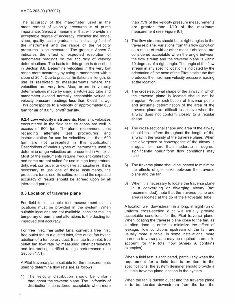
The accuracy of the manometer used in the
measurement of velocity pressures is of prime
importance. Select a manometer that will provide an
acceptable degree of accuracy; consider the range,
slope, quality, scale graduations, indicating fluid of
the instrument and the range of the velocity
pressures to be measured. The graph in Annex G
indicates the effect of expected resolution of
manometer readings on the accuracy of velocity
determinations. The basis for this graph is described
in Section 9.6. Determine velocities in the very low
range more accurately by using a manometer with a
slope of 20:1. Due to practical limitations in length, its
use is restricted to measurements where the
velocities are very low. Also, errors in velocity
determinations made by using a Pitot-static tube and
manometer exceed normally acceptable values at
velocity pressure readings less than 0.023 in. wg.
This corresponds to a velocity of approximately 600
fpm for air of 0.075 lbm/ft3 density.
9.2.4 Low velocity instruments. Normally, velocities
encountered in the field test situations are well in
excess of 600 fpm. Therefore, recommendations
regarding alternate test procedures and
instrumentation for use for velocities less than 600
fpm are not presented in this publication.
Descriptions of various types of instruments used to
determine range velocities are presented in Annex J.
Most of the instruments require frequent calibration,
and some are not suited for use in high temperature,
dirty, wet, corrosive, or explosive atmospheres. If it is
necessary to use one of these instruments, the
procedure for its use, its calibration, and the expected
accuracy of results should be agreed upon by all
interested parties.
9.3 Location of traverse plane
For field tests, suitable test measurement station
locations must be provided in the system. When
suitable locations are not available, consider making
temporary or permanent alterations to the ducting for
improved test accuracy.
For free inlet, free outlet fans, convert a free inlet,
free outlet fan to a ducted inlet, free outlet fan by the
addition of a temporary duct. Estimate free inlet, free
outlet fan flow rate by measuring other parameters
and interpreting certified ratings performance (see
Section 17.1).
A Pitot traverse plane suitable for the measurements
used to determine flow rate are as follows:
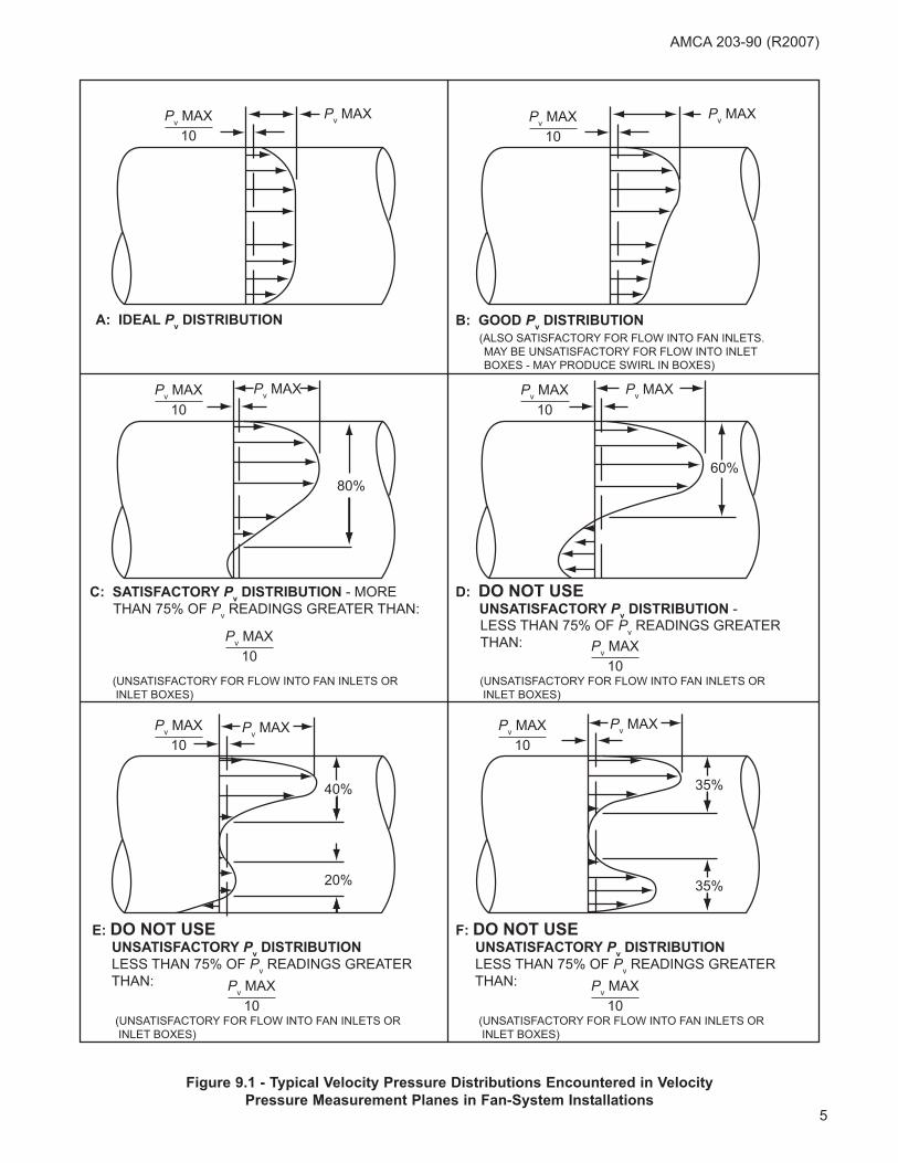
1) The velocity distribution should be uniform
throughout the traverse plane. The uniformity of
distribution is considered acceptable when more
than 75% of the velocity pressure measurements
are greater than 1/10 of the maximum
measurement (see Figure 9.1)
2) The flow streams should be at right angles to the
traverse plane. Variations from this flow condition
as a result of swirl or other mass turbulence are
considered acceptable when the angle between
the flow stream and the traverse plane is within
10 degrees of a right angle. The angle of the flow
stream in any specific location is indicated by the
orientation of the nose of the Pitot-static tube that
produces the maximum velocity pressure reading
at the location.
3) The cross-sectional shape of the airway in which
the traverse plane is located should not be
irregular. Proper distribution of traverse points
and accurate determination of the area of the
traverse plane are difficult to achieve when the
airway does not conform closely to a regular
shape.
4) The cross-sectional shape and area of the airway
should be uniform throughout the length of the
airway in the vicinity of the traverse plane. When
the divergence or convergence of the airway is
irregular or more than moderate in degree,
significantly nonuniform flow conditions may
exist.
5) The traverse plane should be located to minimize
the effects of gas leaks between the traverse
plane and the fan.
6) When it is necessary to locate the traverse plane
in a converging or diverging airway (not
recommended), note that the traverse plane and
area is located at the tip of the Pitot-static tube.
A location well downstream in a long, straight run of
uniform cross-section duct will usually provide
acceptable conditions for the Pitot traverse plane.
When locating the traverse plane close to the fan, as
is often done in order to minimize the effect of
leakage, flow conditions upstream of the fan are
usually more suitable. In some installations, more
than one traverse plane may be required in order to
account for the total flow (Annex A contains
examples).
When a field test is anticipated, particularly when the
requirement for a field test is an item in the
specifications, the system designer should provide a
suitable traverse plane location in the system.
When the fan is ducted outlet and the traverse plane
is to be located downstream from the fan, the
AMCA 203-90 (R2007)
5
AMCA 203-90 (R2007)
Pv MAX Pv MAX
Pv MAX
Pv MAX
Pv MAX
A: IDEAL Pv DISTRIBUTION B: GOOD Pv DISTRIBUTION (ALSO SATISFACTORY FOR FLOW INTO FAN INLETS. MAY BE UNSATISFACTORY FOR FLOW INTO INLET BOXES - MAY PRODUCE SWIRL IN BOXES)
C: SATISFACTORY Pv DISTRIBUTION - MORE THAN 75% OF Pv READINGS GREATER THAN:
D: DO NOT USE UNSATISFACTORY Pv DISTRIBUTION -
(UNSATISFACTORY FOR FLOW INTO FAN INLETS OR INLET BOXES)
(UNSATISFACTORY FOR FLOW INTO FAN INLETS OR INLET BOXES)
(UNSATISFACTORY FOR FLOW INTO FAN INLETS OR INLET BOXES)
LESS THAN 75% OF Pv READINGS GREATER THAN:
F: DO NOT USE UNSATISFACTORY Pv DISTRIBUTION LESS THAN 75% OF Pv READINGS GREATER THAN:
Pv MAX
10Pv MAX
10Pv MAX
10Pv MAX
10Pv MAX
10Pv MAX
10Pv MAX
(UNSATISFACTORY FOR FLOW INTO FAN INLETS OR INLET BOXES)
E: DO NOT USE UNSATISFACTORY Pv DISTRIBUTION LESS THAN 75% OF Pv READINGS GREATER THAN:
10Pv MAX
10Pv MAX
10Pv MAX
10Pv MAX
80%60%
35%40%
20% 35%
Figure 9.1 - Typical Velocity Pressure Distributions Encountered in Velocity
Pressure Measurement Planes in Fan-System Installations
6
AMCA 203-90 (R2007)
Z
MEASUREMENT PLANE
Y
INLET BOX DAMPERS
12 in. MIN.
WHERE: D YZe =
4π
De2
MIN.
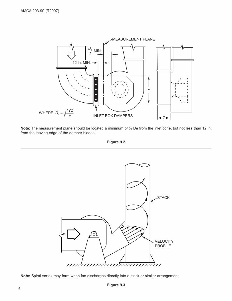
Note: The measurement plane should be located a minimum of ½ De from the inlet cone, but not less than 12 in.
from the leaving edge of the damper blades.
Figure 9.2
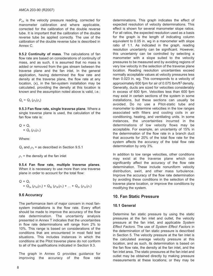
STACK
VELOCITYPROFILE
Note: Spiral vortex may form when fan discharges directly into a stack or similar arrangement.
Figure 9.3

7
traverse plane should be situated a sufficient
distance downstream from the fan to allow the flow to
diffuse to a more uniform velocity distribution and to
allow the conversion of velocity pressure to static
pressure. Annex P provides guidance for the location
of the traverse plane in these cases. The location of
the traverse plane on the inlet side of the fan should
not be less than ½ equivalent diameter from the fan
inlet. Regions immediately downstream from elbows,
obstructions and abrupt changes in airway area are
not suitable traverse plane locations. Regions where
unacceptable levels of swirl are usually present, such
as the region downstream from an axial flow fan that
is not equipped with straightening vanes, should be
avoided. Swirl may form when a fan discharges
directly into a stack or similar arrangement (see
Figure 9.2).
9.3.1 Inlet box location. When the traverse plane
must be located within an inlet box, the plane should
be located a minimum of 12 inches downstream from
the leaving edges of the damper blades and not less
than ½ equivalent diameter upstream from the edge
of the inlet cone (see Figure 9.3). Do not locate
traverse points in the wake of individual damper
blades. In the case of double inlet fans, traverses
must be conducted in both inlet boxes in order to
determine the total flow rate.
9.3.2 Alternative locations. On occasion, an
undesirable traverse plane location is unavoidable, or
each of a limited number of prospective locations
lacks one or more desirable qualities. In such cases,
the alternatives are:
1) Accept the most suitable location and evaluate
the effects of the undesirable aspects of the
location on the accuracy of the test results. In
some instances, the estimated accuracy may
indicate that the results of the test would be
meaningless, particularly in acceptance tests and
proof of performance tests.
2) Provide a suitable location by modifying the
system. This course of action is recommended
for acceptance tests and proof of performance
tests. The modifications may be temporary,
permanent, minor or extensive, depending on the
specific conditions encountered. When the inlet
side of the fan is not ducted but is designed to
accept a duct, consider installing a short length of
inlet duct to provide a suitable traverse plane
location. This duct should be of a size and shape
to fit the fan inlet, a minimum of 2 equivalent
diameters long and equipped with a bell shaped
or flared fitting at its inlet. The traverse plane
should be located a minimum of ½ equivalent
diameters from the fan inlet and not less than 1½
equivalent diameters from the inlet of the duct.
Where the duct is small, its length may
necessarily be greater than 2 equivalent
diameters in order to ensure that the tip of the
Pitot-static tube is a minimum of 1½ equivalent
diameters from the duct inlet. This short length of
duct should produce no significant addition to the
system resistance, but in some cases it may alter
the pattern of flow into the fan impeller, and
thereby affect the performance of the fan slightly.
9.4 The traverse
Annex H contains recommendations for the number
and distribution of measurement points in the
traverse plane. If the flow conditions at the traverse
plane are less than satisfactory, increase the number
of measurement points in the traverse to improve
accuracy.
Since the flow at a traverse plane is never strictly
steady, the velocity pressure measurements
indicated by the manometer will fluctuate. Each
velocity pressure measurement should be mentally
averaged on a time-weighted basis. Any velocity
pressure measurement that appears as a negative
reading is to be considered a velocity pressure
measurement of zero and included as such in the
calculation of the average velocity pressure.
When it is necessary to locate the traverse plane in a
converging or diverging airway, orient the nose of the
Pitot-static tube such that it coincides with the
anticipated line of the flow stream. This is particularly
important at measurement points near the walls of
the airway (see Annex A-1A).
No appreciable effect on Pitot-static tube readings
occur until the angle of misalignment between the
airflow and the tube exceeds 10 degrees.
9.5 Flow rate calculations
9.5.1 Flow rate at traverse plane. The flow rate at
the traverse plane is calculated as follows:
Q3 = V3A3
Where:
A3 = the area of the traverse plane
V3 = the average velocity at the traverse plane
= 1096 (Pv3/ρ3)0.5
ρ3 = the density at the traverse plane
Pv3 = the root mean square velocity pressure at the
traverse plane
= [∑(Pv3r)0.5 / number of readings]2
AMCA 203-90 (R2007)
8
Pv3r is the velocity pressure reading, corrected for
manometer calibration and where applicable,
corrected for the calibration of the double reverse
tube. It is important that the calibration of the double
reverse tube be applied correctly. The use of the
calibration of the double reverse tube is described in
Annex C.
9.5.2 Continuity of mass. The calculations of fan
flow rate are based on considerations of continuity of
mass, and as such, it is assumed that no mass is
added or removed from the gas stream between the
traverse plane and the fan inlet. In the general
application, having determined the flow rate and
density at the traverse plane, the flow rate at any
location, (x), in the fan-system installation may be
calculated, providing the density at this location is
known and the assumption noted above is valid, i.e.:
Qx = Q3 (ρ3/ρx)
9.5.3 Fan flow rate, single traverse plane. Where a
single traverse plane is used, the calculation of the
fan flow rate is:
Q = Q1
= Q3 (ρ3/ρ1)
Where:
Q3 and ρ3 = as described in Section 9.5.1
ρ1 = the density at the fan inlet
9.5.4 Fan flow rate, multiple traverse planes.
When it is necessary to use more than one traverse
plane in order to account for the total flow:
Q = Q1
= Q3a (ρ3a/ρ1) + Q3b (ρ3b/ρ1) + ... + Q3n (ρ3n/ρ1)
9.6 Accuracy
The performance item of major concern in most fan-
system installations is the flow rate. Every effort
should be made to improve the accuracy of the flow
rate determination. The uncertainty analysis
presented in Annex T indicates that the uncertainties
in flow rate determinations will range from 2% to
10%. This range is based on considerations of the
conditions that are encountered in most field test
situations. This includes instances in which the
conditions at the Pitot traverse plane do not conform
to all of the qualifications indicated in Section 9.3.
The graph in Annex G provides guidance for
improving the accuracy of the flow rate
determinations. This graph indicates the effect of
expected resolution of velocity determinations. This
effect is shown for several manometer slope ratios.
For all ratios, the expected resolution used as a basis
for the graph is the length of indicating column
equivalent to 0.05 in. wg in a manometer with slope
ratio of 1:1. As indicated in the graph, reading
resolution uncertainty can be significant. However,
this uncertainty can be controlled by selecting a
manometer with a slope suited to the velocity
pressures to be measured and by avoiding regions of
very low velocity in the selection of the traverse plane
location. Reading resolution uncertainties exceed
normally acceptable values at velocity pressures less
than 0.023 in. wg. This corresponds to a velocity of
approximately 600 fpm for air of 0.075 lbm/ft3 density.
Generally, ducts are sized for velocities considerably
in excess of 600 fpm. Velocities less than 600 fpm
may exist in certain sections of the system in some
installations, but these sections can usually be
avoided. Do no use a Pitot-static tube and
manometer to determine velocities in the low ranges
associated with filters and cooling coils in air
conditioning, heating, and ventilating units. In some
instances, the uncertainties incurred in the
determinations of low velocity flows may be
acceptable. For example, an uncertainty of 15% in
the determination of the flow rate in a branch duct
that accounts for 20% of the total flow rate for the
system affects the accuracy of the total flow rate
determination by only 3%.
In addition to low range velocities, other conditions
may exist at the traverse plane which can
significantly affect the accuracy of the flow rate
determination. These include nonuniform velocity
distribution, swirl, and other mass turbulence.
Improve the accuracy of the flow rate determination
by avoiding these conditions in the selection of the
traverse plane location, or improve the conditions by
modifying the system.
10. Fan Static Pressure
10.1 General
Determine fan static pressure by using the static
pressures at the fan inlet and outlet, the velocity
pressure at the fan inlet, and applicable SystemEffect Factors. The use of System Effect Factors in
the determination of fan static pressure is described
in Section 5. The velocity pressure at the fan inlet is
the calculated average velocity pressure at this
location, and as such, its determination is based on
the fan flow rate, the density at the fan inlet, and the
fan inlet area. The static pressures at the fan inlet and
outlet may be obtained directly by making pressure
measurements at these locations; or they may be
AMCA 203-90 (R2007)

9
determined by making pressure measurements at
other locations, upstream and downstream of the fan.
In the latter case, the determinations must account
for the effects of velocity pressure conversions and
pressure losses, as may occur between the
measurement planes and the planes of interest.
10.2 Pressure measuring instruments
This section describes only the instruments for use in
measuring static pressure. Instruments for use in the
other measurements involved in the determination of
fan static pressure are described in Section 13.
Use a Pitot-static tube of the proportions shown in
Annex B, a double reverse tube as shown in Annex
C, or a side wall pressure tap as shown in Annex E,
and a manometer to measure static pressure.
10.2.1 Pitot-static tube. The comments that appear
in Section 9.2 regarding the use and calibration of the
Pitot-static tube are applicable to its use in the
measurement of static pressures.
10.2.2 Double reverse tube. The double reverse
tube cannot be used to measure static pressure
directly. It must be connected to two manometers and
the static pressure for each point of measurement
must be calculated. Both the manometer connections
and the method of calculation are shown in Annex C.
10.2.3 Pressure tap. The pressure tap does not
require calibration. Use no fewer than four taps
located 90 degrees apart. In rectangular ducts, a
pressure tap should be installed near the center of
each wall. It is important that the inner surfaces of the
duct in the vicinities of the pressure taps be smooth
and free from irregularities, and that the velocity of
the gas stream does not influence the pressure
measurements.
10.2.4 Manometers. A manometer with either
vertical or inclined indicating column may be used to
measure static pressure. Inclined manometers used
to measure static pressures require calibration and
should be selected for the quality, range, slope, scale
graduations, and indicating fluid necessary to
minimize reading resolution errors.
10.3 Static pressure measurements
It is important that all static pressure measurements
be referred to the same atmospheric pressure, and
this atmospheric pressure be that for which the
barometric pressure is determined.
Make static pressure measurements near the fan
inlet and the fan outlet, and where the airway
between the measurement plane and the plane of
interest is straight and without change in cross-
sectional area. Then the duct friction loss between
the measurement plane and the plane of interest is
usually insignificant, and considerations of velocity
pressure conversions and calculations of pressure
losses for duct fitting and other system components
can be avoided.
When a system component is situated between the
measurement plane and the plane of interest, the
pressure loss of the component must be calculated
and credited to the fan. The calculation of the
pressure loss is usually based on the component’s
performance ratings, which may be obtained from the
manufacturer of the item.
If there is a change in area between the
measurement plane and the plane of interest, then
the calculation of the static pressure at the plane of
interest must account for velocity pressure
conversion and include any associated pressure
loss. When the change in area is moderate and
gradual, the conversion of velocity pressure is
considered to occur without loss and the static
pressure is calculated on the basis of no change in
total pressure between the measurement plane and
the plane of interest. This assumes that the duct
friction loss between the two planes is negligible.
When the change in area is an abrupt and sizable
enlargement, as in a duct leading into a large
plenum, the loss is considered to be equivalent to the
velocity pressure in the smaller area, and the static
pressure at the plane of interest is considered to be
the same as the static pressure at the measurement
plane. This assumes that the velocity pressure in the
larger area and the duct friction loss are negligible.
10.3.1 Location of the measuring plane. When the
fan is ducted outlet, the static pressure measurement
plane downstream of the fan should be situated a
sufficient distance from the fan outlet to allow the flow
to diffuse to a more uniform velocity distribution and
to allow the conversion of velocity pressure to static
pressure. See Annex P for guidance in locating the
measurement plane in these cases. In general,
pressure taps should be used if it is necessary to
measure static pressure in the immediate vicinity of
the fan outlet. The static pressure at this location is
difficult to measure accurately with a Pitot-static tube
due to the existence of turbulence and localized high
velocities. If the surface conditions or the velocities at
the duct walls are unsuited for the use of pressure
taps, then a Pitot-static tube must be used with
extreme care, particularly in aligning the nose of the
tube with the lines of the flow streams.
The location of the static pressure measurement
AMCA 203-90 (R2007)
10
plane upstream of the fan should not be less than ½
equivalent diameter from the fan inlet. In the event
that static pressure measurements must be made in
an inlet box, the measurement plane should be
located as indicated in Figure 9.2. In the case of
double inlet fans, static pressure measurements must
be made in both inlet boxes in order to determine the
average static pressure on the inlet side of the fan.
In general, the qualifications for a plane well suited
for the measurement of static pressure are the same
as those for the measurement of velocity pressure,
as indicated in Section 9.3:
1) The velocity distribution should be uniform
throughout the traverse plane.
2) The flow streams should be at right angles to the
plane.
3) The cross-sectional shape of the airway in which
the plane is located should not be irregular.
4) The cross-sectional shape and area of the airway
should be uniform throughout the length of the
airway in the vicinity of the plane.
5) The plane should be located such as to minimize
the effects of leaks in the portion of the system
that is located between the plane and the fan.
A long, straight run of duct upstream of the
measurement plane will usually provide acceptable
conditions at the plane. Regions immediately
downstream from elbows, obstructions, and abrupt
changes in airway area are generally unsuitable
locations. Regions where unacceptable levels of
turbulence are present should be avoided.
If in any fan-system installation the prospective
locations for static pressure measurement planes
lack one or more desirable qualities, the alternatives
are to accept the best qualified locations and
evaluate the effects of the undesirable aspects of the
conditions on the accuracy of the test results or
provide suitable locations by modifying the system.
10.3.2 When using a Pitot-static tube or a double
reverse tube to measure static pressure, a number of
measurements must be made throughout the plane.
Use Annex H to determine the number and
distribution of the measurement points. When using
pressure taps, a single measurement at each of the
taps located at the plane is sufficient.
10.4 Static pressure calculations
Static pressure measurements may be positive or
negative. By definition, positive values are those
measured as being greater than atmospheric
pressures; negative values are those measured as
being less than atmospheric pressure. In all of the
equations in this publication, the values of static
pressures must be entered with their proper signs
and combined algebraically.
10.4.1 Static pressure at measuring planes. The
static pressure at a plane of measurement (x) is
calculated as follows:
Where:
Psxr = the static pressure reading, corrected for
manometer calibration
10.4.2 Static pressure at fan inlet or outlet. The
static pressure at the fan inlet, Ps1, and the static
pressure at the fan outlet, Ps2, may be measured
directly in some cases. In most cases, the static
pressure measurements for use in determining fan
static pressure will not be made directly at the fan
inlet and outlet, but at locations a relatively short
distance upstream from the fan inlet and downstream
from the fan outlet. These static pressure
measurements are designated Ps4 and Ps5,
respectively. Static pressure at the fan inlet, Ps1, is
derived as follows:
Pt4 = Pt1 + ΔP4,1
Where:
Pt4 = the total pressure plane of measurement
Pt1 = the total pressure at the fan inlet
ΔP4,1 = the sum of the pressure losses between the
two planes
These losses (ΔP) include those attributable to duct
friction, duct fittings, other system components, and
changes in airway area. Although ΔP represents a
loss in all cases, it is considered a positive value as
used in the equations in this publication. By
substitution and rearrangement:
Ps1 = Ps4 + Pv4 - Pv1 - ΔP4,1
Similarly, for static pressure at the fan outlet, Ps2:
Pt2 = Pt5 + ΔP2,5
Ps2 = Ps5 + Pv5 - Pv2 + ΔP2,5
PP
sx
sxr
number of readings= ∑
AMCA 203-90 (R2007)

11
Where:
The velocity pressures at the various planes can be
determined from the following general equations for
the velocity pressure at a plane of measurement (x):
Pvx = Pv3 (A3/Ax)2 (ρ3/ρx)
Or:
Pvx = (Qx/1096Ax)2 ρx
Locate the static pressure measurement planes such
that the pressure losses between the measurement
planes and the planes of interest are insignificant.
This will eliminate the uncertainties involved in the
determination of the pressure losses, and the
equations for Ps1 and Ps2 reduce to the following:
Ps1 = Ps4 + Pv4 - Pv1
Ps2 = Ps5 + Pv5 - Pv2
These equations may be used when changes in area
between the measurement planes and the planes of
interest are moderate and gradual, and the pressure
losses associated with conversions of velocity
pressure to static pressure are negligible.
If, in addition to the losses being negligible there are
no changes in the areas between the measurement
planes and the respective planes of interest, then the
equations are further reduced to:
Ps1 = Ps4
Ps2 = Ps5
These equations may also be used when the only
losses between the measurement planes and the
planes of interest are those associated with changes
in area that are abrupt and sizable enlargements in
the direction of flow. This assumes that the velocity
pressure in the larger area is negligible.
10.4.3 Fan static pressure. The equation for fan
static pressure is:
Ps = Ps2 - Ps1 - Pv1 + SEF 1 + SEF 2 + ... + SEF n
Where:
SEF 1, SEF 2, ... SEF n = System Effect Factors that
account for the various System Effects that are
uncorrected and exist at the time of the field test.
10.5 Accuracy
The uncertainty analyses in Annex T indicate that the
uncertainties in fan static pressure determinations
are expected range from 2% to 8%. This range is
based on considerations of the conditions expected
to be encountered in most field test situations.
Improve the accuracy of the fan static pressure
determination by avoiding static pressure
measurement plane locations where turbulence or
other unsteady flow conditions will produce
significant uncertainties in the mental averaging of
pressure readings. Other reading resolution
uncertainties are not as significant in the fan static
pressure determination as in the determination of
flow rate. Generally, static pressure measurements
are much greater in magnitude than velocity pressure
measurements, and the selection of a manometer
that will provide reasonably good accuracy is not
usually a problem.
The uncertainty analyses in Annex T and the
resulting anticipated uncertainty range do not
account for uncertainties that may occur in the
following:
• Determinations of velocity pressure conversions
occurring between the measurement planes and
the planes of the fan inlet or fan outlet. The area
and density values that are involved in these
determinations are usually obtained without
significant uncertainties. However, pressure
losses associated with velocity pressure
conversions are often difficult to determine
accurately.
• Determinations of other pressure losses
occurring between the measurement planes and
the fan inlet or fan outlet. This includes pressure
losses in ducts, duct fittings, and other system
components. The calculations of these losses
are based on the assumption of uniform flow
conditions. This assumption may not be valid,
and the calculated pressure loss values may be
significantly inaccurate.
• Determinations of the values of System EffectFactors. These determinations are based on
limited information, and as such, are subject to
uncertainty.
Avoid situations requiring these determinations,
thereby eliminating them as sources for uncertainties.
The uncertainties involved in determining the values
of System Effect Factors can be avoided only by
correcting the causes of the System Effects. This
requires alterations to the system.
AMCA 203-90 (R2007)

12
11. Fan Power Input
11.1 General
Fan power input data included as part of the fan
performance ratings are normally defined and limited
to either:
• power input to the fan shaft
• the total of the power input to the fan shaft and
the power transmission loss
The losses in fan shaft bearings are included in either
case. Since the results of field tests are usually
compared to the rated performance characteristics of
the fan, field test values of fan power input should be
determined on the same basis as that used in the fan
ratings. For belt driven fans, the rated fan power input
may or may not include belt drive losses. The
information regarding the basis of the rated fan
power input accompanies the rating data or is
otherwise available from the fan manufacturer. In
most instances, when a power transmission loss
occurs, the loss will have to be determined and
subtracted from the motor output in order to obtain
the fan power input.
11.2 Power measurement methods
In view of the fact that accuracy requirements for field
test determinations of fan power input vary
considerably, a number of test methods are
recommended. These methods are intended to
provide economical and practical alternatives for
dealing with various levels of accuracy requirements.
11.2.1 Phase current method. This method for
estimating the power output of three phase motors is
based on the relationship of motor current and motor
power output. The method, described in Annex K,
requires measurements of the phase currents and
voltages supplied to the motor while driving the fan.
Depending on the operating load point of the motor, it
may also involve the measurements of the no load
phase currents.
The phase current method is convenient and
sufficiently accurate for most field tests. In this
method, the closer the actual phase current is to the
motor nameplate value of full load amps, the greater
the accuracy. Since fan motors are normally selected
for operation at or near the full load point, this method
provides a reasonably accurate estimate of the
power output of the fan motor. Determine fan power
input by using the motor power output and, where
applicable, the power transmission loss.
11.2.2 Typical motor performance data. Typical
motor performance data may be used to determine
fan power input. These data, which are referred to as
typical in that the data and the actual performance of
the motor are expected to correspond closely, can
usually be obtained from the motor manufacturer.
The data provided can be in a variety of forms, but
are sufficient to determine motor power output based
on electrical input measurements. It is important that
the power supplied to the motor during the field test
be consistent with that used as the basis for the
motor performance data. The phase voltage should
be stable and balanced, and the average should be
withing 2% of the voltage indicated in the
performance data.
Depending on the form of the typical motor
performance data, motor power output is determined
by one of the following methods:
1) Given the typical motor performance chart ofwatts input versus motor power output at a statedvoltage.
Hmo, is the value in the typical motor performance
data that corresponds to the field test
measurement of watts input to the motor.
2) Given the typical motor performance chart ofwatts input versus torque output and speed at astated voltage.
Use the field test measurement of watts input
and the corresponding typical motor performance
data values of torque output and speed; the
motor power output is calculated as:
3) Given the typical motor performance chart ofwatts input versus motor efficiency at a statedvoltage.
Use the field test measurement of watts input
and the corresponding typical motor performance
data value of motor efficiency, the motor power
output is calculated as:
4) Given the typical motor performance chart ofamps versus power factor and motor efficiency ata stated voltage.
Use the field test measurements of amps input
and volts, and the typical motor performance
data values of power factor (pf) and motor
efficiency, corresponding to the measured amps
input; the motor power output is calculated as:
H watts input motor efficiencymo = ×
746
H T Nmo = ×
63025
AMCA 203-90 (R2007)
13
Or, for three phase motors:
In both equations, amps and volts are the field test
measurement values and, in the case of three phase
motors, are the averages of the measured phase
values.
The fan power input is the motor power output minus
the power transmission loss, where applicable.
11.2.3 Calibrated motors. A calibrated motor may be
used to determine fan power input. When intending
to use this method, it is usually necessary to specify
in the motor purchase arrangements that the motor
be calibrated since an additional cost is normally
involved. Calibration data are similar to typical motor
performance data with the exception that, instead of
being merely typical, the calibration data represent
the performance of a specific motor, based on a test
of the motor. The motor is calibrated over a range of
operation. Electrical input data and other data
sufficient for the determination of power output are
obtained in the calibration. The calibration normally
provides data for operation at nameplate voltage, but
may include data for operation at voltages 10%
greater and 10% less than nameplate voltage. It is
important that the power supplied to the motor during
the field test be consistent with that used in its
calibration. The phase voltage should stable and
balanced, and the average should be within 2% of
the voltage at which the motor was calibrated. The
field test measurements and the calculations
involved in the determination of motor power output
are the same as those described in Section 11.2.2 for
use with typical motor performance data. The fan
power input is the motor power output minus the
power transmission loss, where applicable.
A calibrated motor provides accurate data to
determine motor power output. However, the cost of
the calibration is a limiting factor in the use of this
method in field tests. For low horsepower
applications, the fan manufacturer may be able to
calibrate a motor.
11.2.4. Torquemeters. Another method to determine
fan power input involves the use of a torquemeter
installed between the fan and the driver. The use of a
torquemeter requires some prearrangement with the
purchaser, who would normally have specified such
equipment, so that site conditions can be altered to
accommodate its installation. The torquemeter is
extremely limited in field test application. This is due
mainly to is high cost and the cost of its installation.
In addition, the length of the shut down time and the
revisions to site conditions required for its installation
are usually undesirable. For practical considerations,
it is not normally used in cases where the fan is belt
driven and where the fan impeller is installed directly
on the motor shaft.
11.3 Power measuring instruments
Measurement of current, voltage, watts, and power
factor can be obtained by using an industrial type
power analyzer of good quality. This type of
instrument is available with accuracies of 1% full
scale for volts, amps and power factor, and 2% full
scale for watts. Normally, the higher levels of
accuracy requirements can be met by using this type
of instrument, providing the measurements are well
up on the scales.
In many cases, accuracy level requirements will
permit the use of a clip-on type ammeter-voltmeter.
Clip-on instruments with accuracies of 3% full scale
are available.
11.4 Power transmission losses
Several types of power transmission equipment are
used in driving fans. Those in which power
transmission losses should be considered in the
determination of fan power input include belt drives,
gear boxes, fluid drives, and electromechanical
couplings.
Information as to whether the fan power input ratings
include power transmission losses is included in the
published performance ratings or is otherwise
available from the fan manufacturer. It is important
that this be established and that the fan power input
be determined accordingly in order to provide a valid
comparison of field test results to the fan
performance ratings. In most cases, fan power input
ratings do not include power transmission losses.
11.4.1 Estimating belt drive losses. In view of the
lack of published information available for use in
calculating belt drive losses, a graph is included in
Annex L for this purpose. As indicated in the graph,
belt drive loss, expressed as a percentage of motor
power output, decreases with increasing motor
power output and increases with increasing speed.
This graph is based on the results of over 400 drive
loss tests provided to AMCA by drive manufacturers.
The graph serves as a reasonable guide in
evaluating belt drive losses. The calculation of belt
drive loss, using this graph, is included in many of the
examples in Annex A.
H amps volts pf motor efficiencymo = × × ×
746
H amps volts pf motor efficiencymo = × × × ×( ) .3
746
0 5
AMCA 203-90 (R2007)

14
11.4.2 Estimating other transmission losses. For
other types of power transmission equipment, consult
the fan manufacturer to establish whether
transmission losses are included in the fan ratings,
and if so, request the magnitudes of the losses
allowed in the ratings. Otherwise, it will be necessary
to consult the manufacturer of the power
transmission equipment for the information regarding
transmission losses.
11.5 Accuracy
The uncertainty analyses presented in Annex T
indicate that the uncertainties in fan power input
determinations are expected to range from 4% to 8%.
This range is based on considerations of the
conditions encountered in most field test situations,
estimated accuracies of the various test methods
presented in this publication and allowances for
uncertainties in the determinations of power
transmission losses.
12. Fan Speed
12.1 Speed measuring instruments
Measure speed with a revolution counter and
chronometer, a stroboscopic tachometer, an
electronic counter-timer, or any other precision type
tachometer which has a demonstrated accuracy of
0.5% of the measured value. Friction driven and
magnetic type pickups should not be used in low fan
power ranges where they can influence speed and
fan power input measurements.
12.2 Speed measurements
Establish the speed by averaging a minimum of three
measurements made during the test determination
period. The variation in the measurements should not
exceed 1% for any single point of operation.
13. Densities
13.1 Locations of density determinations
Determine the densities of the gas stream for Plane
1, the fan inlet; and for Plane 3, the velocity pressure
measurement plane. In addition, the density at Plane
2, the fan outlet, must be determined whenever the
fan total pressure, the fan velocity pressure, or an
SEF at the outlet side of the fan is required.
13.2 Data required at each location
The pressure and temperature of the gas stream
must be obtained for each plane at which a density
determination is required. The pressures at Planes 1
and 2 are based on the static pressure
measurements made for the purpose of determining
the fan static pressure. The pressure at Plane 3 is
obtained by averaging static pressure measurements
made concurrent with the velocity pressure
measurements made in a traverse of Plane 3. The
absolute pressure at a plane is calculated by using
the static pressure at the plane and the barometric
pressure. For this reason, it is important that the
barometric pressure be determined for the
atmosphere to which static pressure measurements
are referred. The temperatures used in density
determinations are measured at the planes of
interest.
13.3 Additional data
Additional data required in the determination of
density depends on the gas stream as indicated
below:
1) For air, the wet-bulb temperature is required
unless it is otherwise known that the air is
saturated with water vapor or that the water
vapor content of the air is insignificant. It should
be noted that incorrect assumptions as to
whether the air is dry or saturated can result in
substantial errors in density determinations.
2) For gases other than air, the normal procedure is
to rely on process personnel for the data
necessary to determine the density of the gas.
The information provided will include density or
data sufficient to calculate the density, which
should be for stated conditions of temperature
and pressure.
13.4 Density values
Gas stream density can be established when the
pressure, temperature, and additional data, as
indicated in Section 13.3, have been obtained.
Procedures for establishing density are described in
the examples in Annex M and are further illustrated in
the field test examples in Annex A.
Although the pressure and temperature of the gas
stream must be obtained for each plane at which a
density value is required, it is usually necessary to
obtain additional data, such as the wet-bulb
temperature, for only one plane in order to establish
the densities at all planes. The densities at the planes
for which the additional data is not obtained can be
calculated, providing the gas stream does not change
composition or undergo a change in phase between
planes. The calculation is based on density being
directly proportional to absolute pressure and
AMCA 203-90 (R2007)
15
inversely proportional to absolute temperature.
13.4.1 Example calculation - ρ3 from ρ1. Use Figure
N.1 of Annex N to establish the density of air at Plane
1 based on the test determinations of barometric
pressure, pb, and the following Plane 1 values:
Ps1, static pressure, in. wg
td1, dry-bulb temperature, °F
tw1, wet-bulb temperature, °F
The following data are obtained for Plane 3:
Ps3, static pressure, in. wg
td3, dry-bulb temperature, °F
Calculate the density at Plane 3 as follows:
Where:
p1 = the absolute pressure, in. Hg at Plane 1,
calculated as follows:
p1 = pb + (Ps1/13.6)
In this manner, ρ3 can be calculated without having to
measure the wet-bulb temperature at Plane 3. These
equations can be used for gases other than air and
can be adapted for use in calculations involving any
two planes, subject to the limitations noted earlier.
In the example calculation of ρ3, pb is determined for
the atmosphere to which the measurements of Ps1
and Ps3 are referred. Refer static pressure
measurements to a common atmosphere. When
the pressures cannot be referred to a common
atmosphere, the absolute pressure for each plane is
calculated by using the static pressure measurement
at the plane and the barometric pressure for the
atmosphere to which the static pressure
measurement is referred. However, for the purposes
of accuracy, static pressure measurements that are
used in the determination of fan static pressure must
be referred to a common atmosphere.
13.5 Temperatures
Measure temperatures with mercury-in-glass, dial, or
thermocouple type thermometers. For temperatures
through 220°F, the thermometer should be accurate
within 2°F of the measured value and readable to 1°F
or finer. For temperatures above 220°F, the
thermometer should be accurate within 5°F of the
measured value and readable to 5°F or finer.
The temperature determination should be
representative of the average temperature of the gas
stream throughout the plane of interest. When the
temperature varies with time or temperature
stratification exists at the measurement plane,
several temperature measurements may be
necessary in order to obtain a representative
average. At elevated temperatures, the thermometer
may have to be shielded to prevent radiation effects
from exposed heat sources.
Locate the wet-bulb thermometer downstream from
the dry-bulb thermometer in order to prevent the dry-
bulb temperature measurement from being adversely
affected. The wet-bulb thermometer wick should be
clean, closely fitted, and wetted with fresh water. The
velocity of the air over the wick should be between
700 and 2000 fpm. Use a sling psychrometer to
obtain dry and wet-bulb air temperature
measurements at the fan inlet for free inlet fans.
13.6 Barometric pressure
Use a portable aneroid barometer for field test
determinations of barometric pressure when an
acceptable site barometer is not available. The
barometer should be accurate within 0.05 in. Hg of
the measured value. Determine the test value of
barometric pressure by averaging measurements
made at the beginning and end of the test period.
When the test value of barometric pressure is to be
based on data obtained from a nearby airport, it is
important that the data include the barometric
pressure for the airport site and the elevation for
which the pressure was determined (often the
barometric pressure is corrected to sea level). This
pressure value must then be corrected to the test site
elevation. Barometric pressure decreases
approximately 0.1 in. Hg for every 100 ft increase in
elevation
13.7 Accuracy
As indicated in Annex T, uncertainties in density
determinations are expected to be less than 3%.
However, care must be exercised in obtaining
representative test measurements in order to prevent
the uncertainties from exceeding this value.
14. Conversion Calculations
Generally, the test fan will be operating at a speed
and inlet density that are somewhat different from the
ρ ρ3 1
13 6
13 6
460
460= +⎛
⎝⎜
⎞
⎠⎟
++
⎛
⎝⎜
⎞
⎠⎟
P pp
tt
s3 b
1
d1
d3
.
.
AMCA 203-90 (R2007)
16
fan performance rating values of fan speed and inlet
density. In order to provide a common basis for
comparing the field test results to the fan
performance ratings, each of these two items must
be the same in both sets of data. This can be
accomplished by converting the results of the field
test to the speed and density conditions of the fan
performance ratings. The equations for the
conversion are as follows.
Qc = Q (Nc / N)
Psc = Ps (Nc / N)2 (ρc / ρ)
Ptc = Pt (Nc / N)2 (ρc / ρ)
Pvc = Pv (Nc / N)2 (ρc / ρ)
Hc = H (Nc / N)3 (ρc / ρ)
Where the subscript c designates values converted
to specified conditions, and items without the
subscript c are field test values.
These conversion equations do not account for the
effect of the compressibility of the gas stream.
However, since the test fan usually operates at
conditions of speed and inlet density that are
reasonably close to the quoted fan performance, the
conversion calculations usually result in small
changes from field test values and the effect of the
compressibility of the gas stream is considered to be
negligible. Where test conditions are considerably
different than design conditions, the effect of
compressibility may need to be considered.
15. Test Preparation
15.1 The following items should be agreed upon by
all interested parties prior to the start of a field
performance test:
1) AMCA Publication 200, Air Systems, AMCA
Publication 201, Fans and Systems, and AMCA
Publication 202, Troubleshooting, should be
reviewed and implemented before starting the
field test.
2) Personnel conducting field tests on fans must be
technically competent and fully conversant with
all four parts of the AMCA Fan Application
Manual. The person responsible for conducting
the test should be designated and agreed upon
by all parties.
3) The test instrumentation and locations of test
measurement planes should be established.
Work required to accommodate test
measurements (drilling of traverse holes,
installation of static pressure taps and
thermometer wells, etc.) should be completed
prior to the test date.
4) System Effect Factors, if any, must be
established prior to the conduct of the test.
5) The expected test uncertainties must be agreed
upon prior to the test (see Annex T).
6) Responsibility for the cost of the test or any fan-
system modifications required as a result of the
test should be established.
7) Prior to testing, an inspection must be made to
ensure that the fan is installed in accordance with
the fan manufacturer’s recommendations. The
duct system should also be inspected for
compliance with design specifications, conditions
of filters, abnormal duct restrictions, etc.
8) The majority of fan field performance tests cover
a single point of operation, namely, the design
duty. If it is deemed necessary to cover several
points of operation, provision must be made in
advance for changing the system resistance. The
means used to vary the system resistance must
not cause adverse flow conditions in the vicinities
of the fan and measurement planes. If the fan
cannot be tested at the quoted system design
point, then it is sufficient for the evaluation of fan
field performance to establish the proximity of the
field test point to any portion of the fan
performance rating curve within the limitations of
the uncertainty analysis (see Annex T).
9) It must be established that the system remains
constant for the duration of the test. Modulating
dampers should be set in a fixed position, no
process changes shall be undertaken, etc.
Variable inlet vane controls or inlet box dampers
must be set in the full open position for the
duration of the test, except when testing for
control characteristics.
10) All precautions to ensure the safety of test
personnel must be observed.
11) The fan-system should be operated for a length
of time sufficient to ensure steady state
conditions prior to the start of the test.
12) It is advisable that representatives of all parties
interested in the test results be present at the
time of the test to cover their areas of
responsibility.
AMCA 203-90 (R2007)
17
15.2 It is recommended that as a minimum, the
following equipment be taken to or be otherwise
available at the job site:
1) Pitot-static tubes of suitable lengths for the
maximum duct size to be traversed.
Considerations should be given to the use of a
double reverse tube in dirty atmospheres.
2) Manometers suitable for measuring static
pressures. Manometer fluids other than water are
acceptable, provided the specific gravity is
known. A spare bottle of manometer fluid is
advisable.
3) Inclined manometer suitable for measuring
velocity pressures.
4) Flexible tubing of suitable length to enable
manometers to be installed at a convenient
location.
5) Tubing couplings and “T” type tubing connectors.
6) Thermometers to cover the range of anticipated
temperatures.
7) Sling psychrometer for obtaining dry-bulb and
wet-bulb temperatures.
8) Clip-on ammeter-voltmeter, power analyzer, or
other suitable electrical measurement
instruments for the determination of fan power
input.
9) Fan speed measurement instrument.
10) Aneroid barometer.
11) Flashlight, tape, measuring rule, hand tools,
coveralls, etc.
12) Test data sheets, calculator, and necessary
drawings.
13) Complete AMCA Fan Application Manual
containing Publications 200, 201, 202, and 203.
16. Precautions
The following precautions should be observed when
conducting a field test:
1) Connect the Pitot-static tube to the manometers
according to anticipated pressures, i.e., whether
the pressures are positive or negative, and the
magnitudes of pressures.
2) Static and total pressure manometer tubing must
be “pinched off” prior to inserting or removing the
Pitot-static tube from the test duct. Release both
legs of the tubing simultaneously after the Pitot-
static tube is inside the test duct and properly
oriented. Failure to release simultaneously may
result in manometer fluid being blown from the
manometer.
3) Loop the manometer tubing well above the
manometer so that any fluid which is
inadvertently blown from the gauge will drain
back into the manometer.
4) The Pitot-static tube is intended for measuring
pressures in relatively clean gases. When using
Pitot-static tubes in dirty, wet, or corrosive
atmospheres, both legs of the Pitot-static tube
must be cleaned out frequently during the test.
Since fan pressure readings are never strictly
steady, absence of fluctuations is an
indication of a plugged Pitot-static tube.
Consider using a double reverse tube in these
situations.
5) When making measurements in wet gas
streams, continually check for the presence of
moisture in the tubing. Clear plastic tubing is
ideal from this standpoint. If moisture collects in
the tubing, immediately remove the Pitot-static
tube and clean the inside of the tubing and Pitot-
static tube before proceeding with the test.
6) Before performing any work inside a fan,
ductwork, or other system components, make
certain that the fan motor starter is “locked out.”
7) The area at the plane of flow measurement
should be measured internally to account for
internal insulation or other obstructions.
8) Do not rely on damper control indicators to
ensure that dampers are fully open. Check
visually.
9) Measure temperatures on both sides of double
inlet fans as temperature differences may exist
between each side.
10) When measuring in high temperature, corrosive
or explosive atmospheres, instruments should be
selected for suitability for such atmospheres.
17. Typical Fan-System Installations
A fan assembly may include any number of
appurtenances: variable inlet vanes, inlet boxes, inlet
AMCA 203-90 (R2007)

18
box dampers, outlet dampers, inlet screens, belt
guards, inlet bells, diffusers (evasés). Alternately,
these items may be included in the fan-system
installation, but not be a part of the fan assembly. In
order to determine the proper field test procedure
and to provide a valid basis for comparing field test
results to the fan performance ratings, it is important
to establish which of these items are considered a
part of the fan and which are considered a part of the
system. The fan performance ratings may be
assumed to include the appurtenances that are
established as being a part of the fan assembly.
The locations of the fan inlet and fan outlet depend
on whether specific appurtenances are considered
to be a part of the fan assembly. If the assembly
includes an inlet box, the fan inlet is the inlet to the
inlet box. For a fan assembly that includes a diffuser,
the fan outlet is the outlet of the diffuser.
In the case of heating, ventilating, and air-
conditioning equipment, the field test procedure will
depend on whether the equipment is a factory
assembled central station unit, a built-up unit, or a
packaged unit (see Section 17.4).
The performance ratings for a fan that includes inlet
box dampers, variable inlet vanes or outlet dampers
cover operation of the fan with these items in the full
open positions. In order to be able to compare the
field test results to the fan performance ratings, it is
essential that these items be fixed in their full open
positions for the duration of the test. In addition, when
the loss through a damper must be calculated, it is
essential that the damper blades be fixed in their full
open positions during the test since this is the
condition on which the damper pressure loss ratings
are based. This consideration arises when a damper,
which is not considered a part of the fan is located
between a static pressure measurement plane and
the fan. In order to determine the fan static pressure,
the loss through the damper must be calculated. In
these cases, the calculation of the loss is based on
the performance ratings for the damper.
17.1 Free inlet, free outlet fans
It is difficult to achieve an accurate field test of a free
inlet, free outlet fan. The most obvious problem is the
lack of a suitable location for the velocity pressure
measurement plane. In addition, in the case of
ventilators that supply or exhaust air from a building-
the most commonly encountered applications of free
inlet, free outlet fans-it is extremely difficult to define,
set, and maintain for the duration of the test the
“normal” system condition. Items affecting the system
include:
a) The operations of ovens, furnaces, paint booths,
air conditioning equipment, other fans, and
similar items that may supply or exhaust air from
the building in intermittent or modulating
fashions.
b) The use of doors providing access to the
building. The effect is most significant when large
doors that are normally closed are kept open for
extended periods such as in loading operations.
c) The velocity and direction of the wind outside the
building, particularly in conjunction with the item
immediately above and as it may affect the flow
of air from the outlet of the ventilator.
d) The use of interior doors that my restrict the flow
of air from areas normally expected to be
ventilated.
Assuming that these difficulties can be resolved and
the desired system is fixed for the duration of the test,
determine the fan performance by using one of the
following methods:
1) Make field test measurements sufficient for
determining fan static pressure, fan power input,
fan speed, and the density of the air at the fan
inlet. In this method for testing a free inlet, free
outlet fan, the fan static pressure is calculated as
the static pressure on the outlet side of the fan
less the static pressure on the inlet side of the
fan: Ps = Ps2 - Ps1. The static pressure
measurements involved must be referred to the
same atmospheric pressure and made at
locations sufficiently distant from the fan inlet and
outlet so as to be unaffected by the velocity of the
air entering and leaving the fan. Using the fan
manufacturer’s certified performance ratings,
draw a performance curve for the fan for
operation at the test values of fan speed and
entering air density. Determine the fan air flow
rate by entering this curve at the test values of
fan static pressure and fan power input (see
Example 5C in Annex A).
2) Use the method as described above with the
exception that the performance curve is
established by a laboratory test of the fan,
conducted in accordance with AMCA Standard
210. For the laboratory test, the fan must be set
up in a manner that duplicates the field
installation conditions. That is, all appurtenances
must be in place and any restrictions or
obstructions to the free flow of air into the fan
inlet and away from the fan outlet must be
accurately duplicated in the laboratory test setup.
AMCA 203-90 (R2007)

19
3) Install a duct on the inlet side of the fan for the
purpose of providing a location for the velocity
pressure measurement plane. All of the test
measurements and calculations in this method
for testing a free inlet, free outlet fan are the
same as those required for a fan with a ducted
inlet and a free outlet. The cross-sectional shape
and area of the duct, which is temporarily
installed for purposes of the test, should be
selected on the basis of minimizing its
interference with the flow of air into the fan inlet
while providing velocity pressure of magnitudes
that can be accurately measured. The length of
the duct should be a minimum of twice its
diameter or equivalent diameter, and the
entrance to the duct should be flared in order to
reduce the entrance loss. The velocity pressure
measurement plane should be located a
minimum of 1.5 diameters or equivalent
diameters downstream from the duct inlet. The
effect of this duct on the system is negligible, but
in changing the pattern of the flow of air into the
fan inlet, it may affect the performance of the fan
slightly. Applications of this method of test are
presented in Examples 5A and 5B in Annex A.
The equation for calculating fan static pressure
for this configuration is:
Ps = Ps2 - (Ps1 + Pv1)
17.2 Free inlet, ducted outlet fans
In the calculation of fan static pressure for this type of
fan-system configuration, the sum of the static
pressure at the fan inlet, Ps1, and the velocity
pressure at the fan inlet, Pv1, is considered to be
equal to the sum of the static pressure, Psx, and the
velocity pressure, Pvx, at a point sufficiently distant
from the fan inlet as to be in still air. At this point, the
static pressure is zero, and the velocity pressure in
still air is zero.
Ps1 + Pv1 = Psx + Pvx = 0
This consideration, which is the same as that used in
the methods for testing fans for performance rating
purposes, charges to the fan the losses incurred in
accelerating the air into the fan inlet and eliminates
inaccuracies which may occur in any attempt to
measure velocity pressure and static pressure at the
fan inlet. Since Ps1 + Pv1 = 0, the equation for
calculating fan static pressure for this configuration
is:
Ps = Ps2 + SEF 1 +SEF 2 + ... + SEF n
17.3 Ducted inlet, ducted outlet fans
In this type of fan-system configuration, there is no
special consideration in the calculation of fan static
pressure. The equation for this calculation is:
Ps = Ps2 - Ps1 - Pv1 + SEF 1 + SEF 2 + ... + SEF n
In this configuration, the flow conditions on the inlet
side of the fan are usually more favorable for the
location of the velocity pressure measurement plane.
17.4 Ducted inlet, free outlet fans
In this type of fan-system configuration, the static
pressure at the fan outlet, Ps2, is zero gauge
pressure, referred to the atmospheric pressure in the
region of the fan outlet. However, the gas stream may
be discharging from the fan into a region in which the
atmospheric pressure is somewhat different from that
to which all other pressure measurements are
referred. When this possibility exists, it is essential
that the static pressure measurements in the region
of the fan outlet be referred to the same atmospheric
pressure as used in all other pressure
measurements.
Ps = -Ps1 - Pv1 + SEF 1 + SEF 2 + ... + SEF n
17.5 Air handling units
This category consists of draw-through and blow-
through types of equipment assemblies used in
heating, ventilating, and air-conditioning applications.
In addition to fans, these equipment assemblies may
include any number of combinations of coils, filters,
access sections, humidifiers, mixing boxes, dampers,
etc. Air handling units include packaged units, factory
assembled central station units, and built-up units.
The basis used in establishing the air performance
ratings for each of these unit types is described
below. It is important that the field test method
correspond to the rating method in each case.
17.5.1 Packaged units. This type of unit is supplied
and rated by the manufacturer as an assembly. The
static pressures at the inlet and outlet to the
assembly and the velocity pressure at the inlet to the
assembly are used in calculating the static pressure
generated by this type of air handling unit. See
Examples 4C and 4D in Annex A.
17.5.2 Factory assembled central station units.
The air performance ratings for this type of unit are
based on the operation of the fan section assembly
only, but include the effects of the air flow conditions
AMCA 203-90 (R2007)
20
entering and leaving the fan section which are
created by accessory equipment such as plenums,
coils, filters, mixing boxes, etc. The fan section
assembly includes the fan and the cabinet in which
the fan has been installed. The accessory items are
considered to be included in the system in which the
fan section operates. The static pressure and the
velocity pressure at the inlet of the fan section and
the static pressure at the fan section outlet, which
coincides with the fan outlet, are used in calculating
the static pressure generated by the fan section
assembly. See examples 4B and 4E in Annex A.
17.5.3 Built-up units. Built-up units are similar to
factory assembled central station units, except that in
built-up units, the components are normally obtained
from a number of equipment suppliers and the unit is
assembled at the installation site. The fans which are
used in built-up units are rated as free-standing,
unencumbered by the cabinets in which they are
installed. In the field test determination of the
performance of the fan, the static pressure and
velocity pressure at the fan inlet and the static
pressure at the fan outlet are used in calculating the
fan static pressure. An SEF that accounts for the
effect of the cabinet is normally included in this
calculation, and it may be necessary to include an
SEF to account for the conditions at the fan outlet.
See Example 4A in Annex A.
AMCA 203-90 (R2007)

21
AMCA 203-90 (R2007)
Annex A. Field Test Examples
This annex contains examples of field tests. The examples are presented in detail and cover several types of fan-
system combinations. Field test procedures are illustrated in a variety of situations. Portions of the procedures are
typical for all fan-system installations. Other portions of the procedures demonstrate methods for dealing with the
more difficult features encountered in some installations. Not all of the possible fan-system combinations are
included in the examples, but it is expected that the examples will provide sufficient guidance for dealing with those
cases not covered.
EXAMPLES OF FANS, INSTALLATION TYPE B: FREE INLET, DUCTED OUTLET
1A: Centrifugal Forced Draft Fan
1B: Centrifugal Forced Draft Fan with Inlet Silencers
1C: Axial Forced Draft Fan with Inlet Silencers
1D: Centrifugal Fans in Parallel
EXAMPLE OF FANS, INSTALLATION TYPE D: DUCTED INLET, DUCTED OUTLET
2A: Utility Fan in a Ventilating System
2B: Centrifugal Fan in a Sawdust Conveying System
2C: Axial Fan in a Dryer System
2D: Centrifugal Fan in a Scrubber System
2E: Centrifugal Fan in a Process System
2F: Axial Fan in a Ventilation System
2G: High Pressure Centrifugal Fans in Series
EXAMPLES OF FANS, INSTALLATION TYPE C: DUCTED INLET, FREE OUTLET
3A: Centrifugal Fan in an Exhaust System
3B: Axial Fan in an Exhaust System
3C: Centrifugal Fan in a Scrubber System
3D: Centrifugal Roof Ventilator with Ducted Inlet
EXAMPLES OF AIR HANDLING UNITS
4A: Centrifugal Fan in a Built-up Air conditioning Unit
4B: Central Station Air Conditioning Unit, Factory Assembled Draw-Through Type
4C: Packaged Air Conditioning Unit
4D: Packaged Air Conditioning Unit
4E: Central Station Air Conditioning Unit, Factory Assembled Blow-Through Type
EXAMPLES OF FANS, INSTALLATION TYPE A: FREE INLET, FREE OUTLET
5A: Free Inlet, Free Outlet Roof Ventilator with temporary duct
5B: Free Inlet, Free Outlet Propeller Fan with temporary duct
5C: Free Inlet, Free Outlet Roof Ventilator as installed
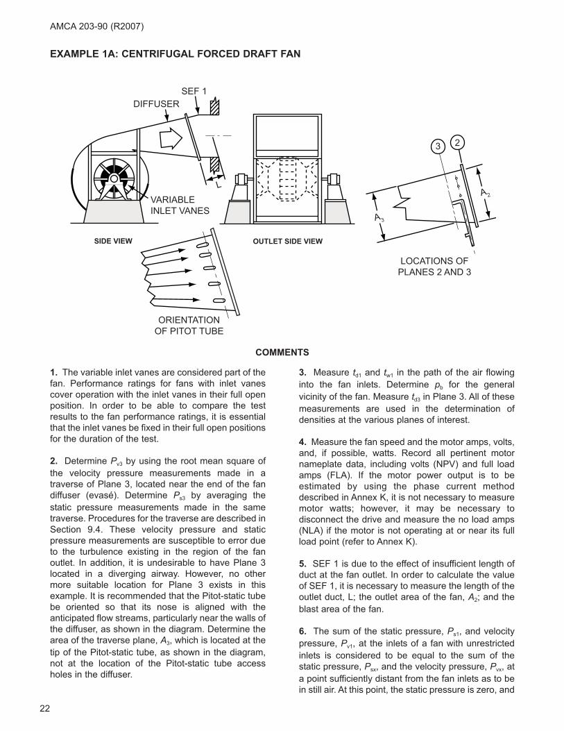
22
AMCA 203-90 (R2007)
1. The variable inlet vanes are considered part of the
fan. Performance ratings for fans with inlet vanes
cover operation with the inlet vanes in their full open
position. In order to be able to compare the test
results to the fan performance ratings, it is essential
that the inlet vanes be fixed in their full open positions
for the duration of the test.
2. Determine Pv3 by using the root mean square of
the velocity pressure measurements made in a
traverse of Plane 3, located near the end of the fan
diffuser (evasé). Determine Ps3 by averaging the
static pressure measurements made in the same
traverse. Procedures for the traverse are described in
Section 9.4. These velocity pressure and static
pressure measurements are susceptible to error due
to the turbulence existing in the region of the fan
outlet. In addition, it is undesirable to have Plane 3
located in a diverging airway. However, no other
more suitable location for Plane 3 exists in this
example. It is recommended that the Pitot-static tube
be oriented so that its nose is aligned with the
anticipated flow streams, particularly near the walls of
the diffuser, as shown in the diagram. Determine the
area of the traverse plane, A3, which is located at the
tip of the Pitot-static tube, as shown in the diagram,
not at the location of the Pitot-static tube access
holes in the diffuser.
3. Measure td1 and tw1 in the path of the air flowing
into the fan inlets. Determine pb for the general
vicinity of the fan. Measure td3 in Plane 3. All of these
measurements are used in the determination of
densities at the various planes of interest.
4. Measure the fan speed and the motor amps, volts,
and, if possible, watts. Record all pertinent motor
nameplate data, including volts (NPV) and full load
amps (FLA). If the motor power output is to be
estimated by using the phase current method
described in Annex K, it is not necessary to measure
motor watts; however, it may be necessary to
disconnect the drive and measure the no load amps
(NLA) if the motor is not operating at or near its full
load point (refer to Annex K).
5. SEF 1 is due to the effect of insufficient length of
duct at the fan outlet. In order to calculate the value
of SEF 1, it is necessary to measure the length of the
outlet duct, L; the outlet area of the fan, A2; and the
blast area of the fan.
6. The sum of the static pressure, Ps1, and velocity
pressure, Pv1, at the inlets of a fan with unrestricted
inlets is considered to be equal to the sum of the
static pressure, Psx, and the velocity pressure, Pvx, at
a point sufficiently distant from the fan inlets as to be
in still air. At this point, the static pressure is zero, and
EXAMPLE 1A: CENTRIFUGAL FORCED DRAFT FAN
ORIENTATIONOF PITOT TUBE
23
A2
A3
LOCATIONS OFPLANES 2 AND 3
OUTLET SIDE VIEWSIDE VIEW
VARIABLEINLET VANES
DIFFUSERSEF 1
L
COMMENTS
23
the velocity pressure in still air is zero.
Ps1 + Pv1 = Psx + Pvx = 0
This consideration, which is the same as that used in
the methods for testing fans for performance rating
purposes, charges to the fan losses incurred in
accelerating the air into the fan inlets and eliminates
the inaccuracies which arise in any attempt to
measure the velocity pressure and static pressure at
the fan inlets. To calculate the fan static pressure:
Ps = Ps2 - Ps1 - Pv1 + SEF 1
= Ps2 - (Ps1 + Pv1) + SEF1
Since:
Ps1 + Pv1 = 0
Ps = Ps2 + SEF 1
7. In order to compare the test results to the quoted
fan curve drawn for operation at 1780 rpm and
0.0701 lbm/ft3 density, it is necessary to convert the
results to the specified conditions. In this case, the
test conditions are identical to the specified
conditions and no calculations are required.
OBSERVATIONS
SITE MEASUREMENTS
pb = 28.91 in. Hg
td1 = 85°F
tw1 = 63°F
td3 = 96°F
Ps3 = 14.4 in. wg
Pv3 = 1.52 in. wg
N = 1780 rpm
A2 = 11.94 ft2
A3 = 11.3 ft2
Blast Area = 7.76 ft2
L = 3 ft.
MEASURED MOTOR DATA
Volts = 570, 560, 572
= 567 av.
Amps = 160, 166, 163
= 163 av.
MOTOR NAMEPLATE DATA
200 hp, 3 phase, 60 hertz
575 volts, 1800 rpm, 181 FLA
GENERAL
VIVs in full open positions.
Fan direct connected to motor.
CALCULATIONS
DENSITIES
For fan inlet conditions of:
td1 = 85°F
tw1 = 63°F
p1 = pb
= 28.91 in. Hg
Use Figure N.1 in Annex N to obtain ρ1 = 0.0701
lbm/ft3
The density at Plane 3:
In this case, ρ2 is considered to be equal to ρ3.
FLOW RATES
V3 = 1096 (Pv3/ρ3)0.5
= 1096 (1.52/0.0712)0.5
= 5064 fpm
Q3 = V3A3
= 5064 × 11.3
= 57223 cfm
Q = Q1
= Q3 (ρ3/ρ1)
= 57223 (0.0712/0.0701)
= 58121 cfm
FAN POWER INPUT
Measured amps/FLA = (163/181)
= 0.90
= 90%
Annex K indicates that Equation A will provide a
reasonably accurate estimate of motor power output
for a 200 hp motor operating at 90% FLA.
ρ ρ3 1
1
13 6
13 6
460
460
0 070114 4
= +⎛
⎝⎜
⎞
⎠⎟
++
⎛
⎝⎜
⎞
⎠⎟
=
P pp
tt
s3 b d1
d3
.
.
.. ++ ×
×⎛⎝⎜
⎞⎠⎟⎛⎝⎜
⎞⎠⎟
=
13 6 28 91
13 6 28 91
545
556
0 0712 3
. .
. .
. lbm/ft
AMCA 203-90 (R2007)
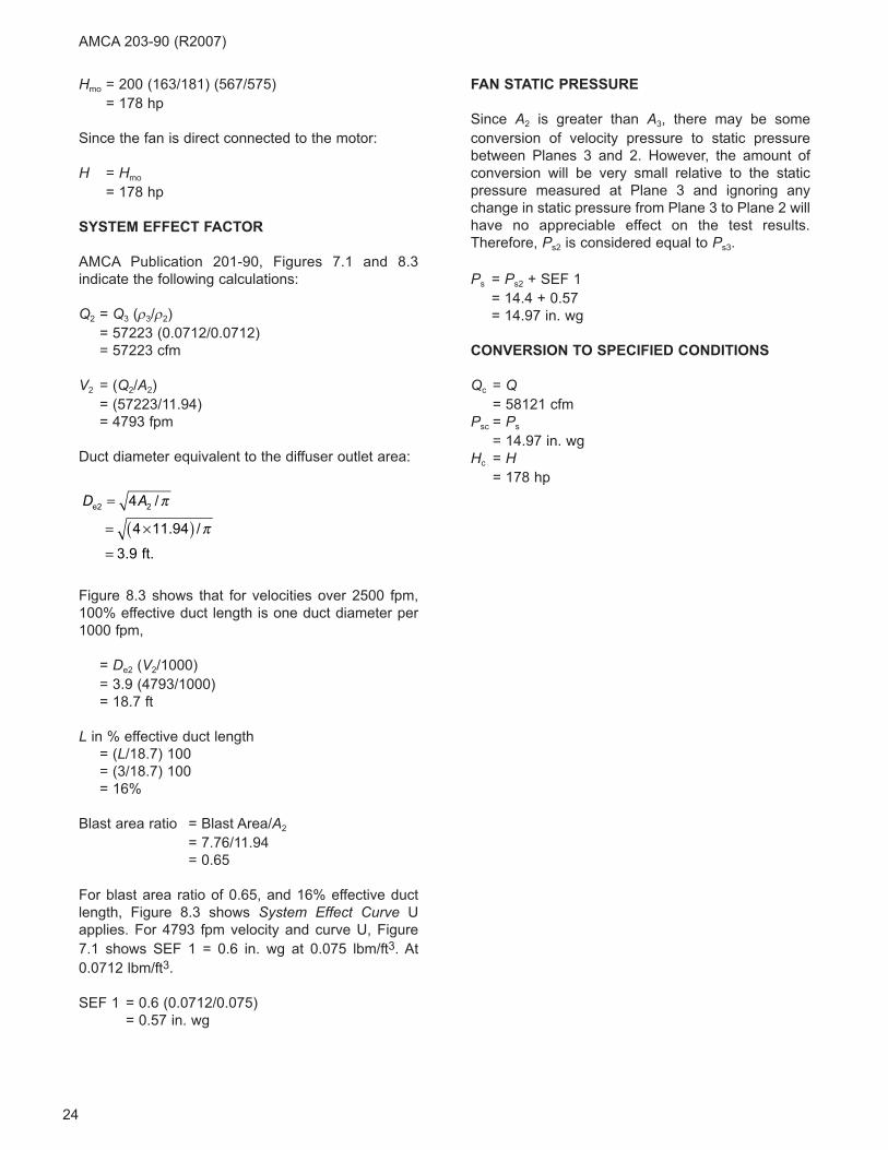
24
Hmo = 200 (163/181) (567/575)
= 178 hp
Since the fan is direct connected to the motor:
H = Hmo
= 178 hp
SYSTEM EFFECT FACTOR
AMCA Publication 201-90, Figures 7.1 and 8.3
indicate the following calculations:
Q2 = Q3 (ρ3/ρ2)
= 57223 (0.0712/0.0712)
= 57223 cfm
V2 = (Q2/A2)
= (57223/11.94)
= 4793 fpm
Duct diameter equivalent to the diffuser outlet area:
Figure 8.3 shows that for velocities over 2500 fpm,
100% effective duct length is one duct diameter per
1000 fpm,
= De2 (V2/1000)
= 3.9 (4793/1000)
= 18.7 ft
L in % effective duct length
= (L/18.7) 100
= (3/18.7) 100
= 16%
Blast area ratio = Blast Area/A2
= 7.76/11.94
= 0.65
For blast area ratio of 0.65, and 16% effective duct
length, Figure 8.3 shows System Effect Curve U
applies. For 4793 fpm velocity and curve U, Figure
7.1 shows SEF 1 = 0.6 in. wg at 0.075 lbm/ft3. At
0.0712 lbm/ft3.
SEF 1 = 0.6 (0.0712/0.075)
= 0.57 in. wg
FAN STATIC PRESSURE
Since A2 is greater than A3, there may be some
conversion of velocity pressure to static pressure
between Planes 3 and 2. However, the amount of
conversion will be very small relative to the static
pressure measured at Plane 3 and ignoring any
change in static pressure from Plane 3 to Plane 2 will
have no appreciable effect on the test results.
Therefore, Ps2 is considered equal to Ps3.
Ps = Ps2 + SEF 1
= 14.4 + 0.57
= 14.97 in. wg
CONVERSION TO SPECIFIED CONDITIONS
Qc = Q= 58121 cfm
Psc = Ps
= 14.97 in. wg
Hc = H= 178 hp
D Ae2
ft.
=
= ×( )=
4
4 11 94
3 9
2 /
. /
.
π
π
AMCA 203-90 (R2007)
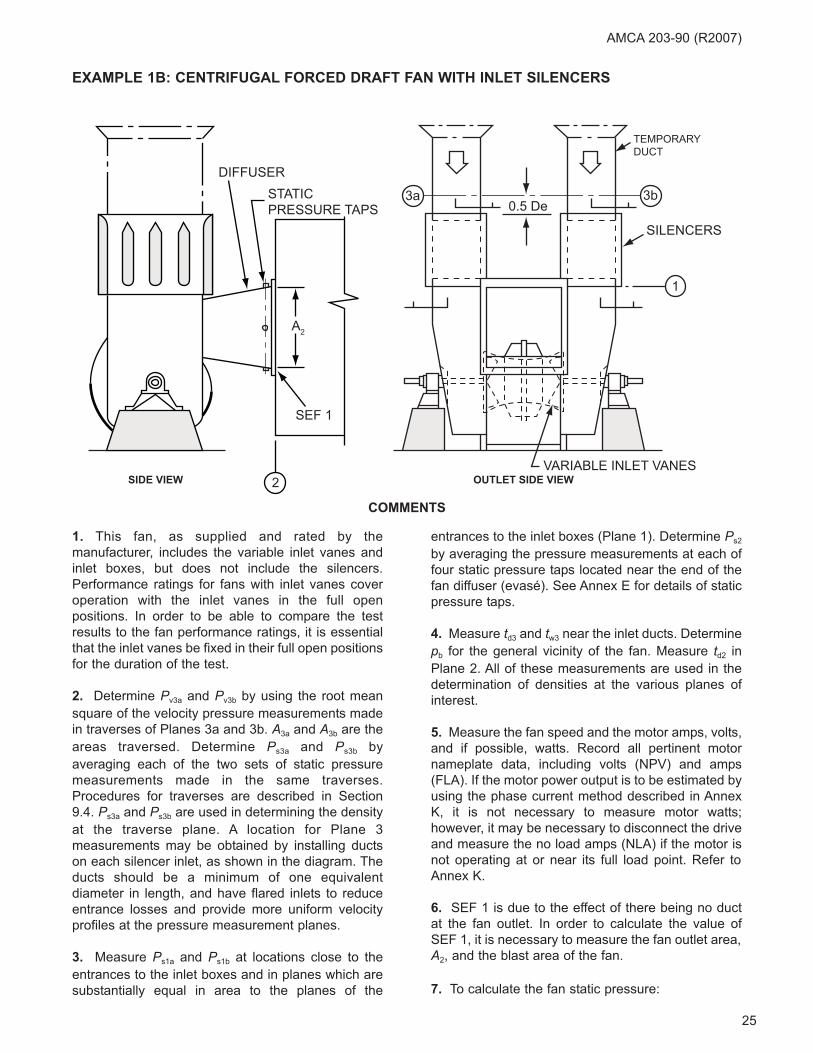
25
AMCA 203-90 (R2007)
1. This fan, as supplied and rated by the
manufacturer, includes the variable inlet vanes and
inlet boxes, but does not include the silencers.
Performance ratings for fans with inlet vanes cover
operation with the inlet vanes in the full open
positions. In order to be able to compare the test
results to the fan performance ratings, it is essential
that the inlet vanes be fixed in their full open positions
for the duration of the test.
2. Determine Pv3a and Pv3b by using the root mean
square of the velocity pressure measurements made
in traverses of Planes 3a and 3b. A3a and A3b are the
areas traversed. Determine Ps3a and Ps3b by
averaging each of the two sets of static pressure
measurements made in the same traverses.
Procedures for traverses are described in Section
9.4. Ps3a and Ps3b are used in determining the density
at the traverse plane. A location for Plane 3
measurements may be obtained by installing ducts
on each silencer inlet, as shown in the diagram. The
ducts should be a minimum of one equivalent
diameter in length, and have flared inlets to reduce
entrance losses and provide more uniform velocity
profiles at the pressure measurement planes.
3. Measure Ps1a and Ps1b at locations close to the
entrances to the inlet boxes and in planes which are
substantially equal in area to the planes of the
entrances to the inlet boxes (Plane 1). Determine Ps2
by averaging the pressure measurements at each of
four static pressure taps located near the end of the
fan diffuser (evasé). See Annex E for details of static
pressure taps.
4. Measure td3 and tw3 near the inlet ducts. Determine
pb for the general vicinity of the fan. Measure td2 in
Plane 2. All of these measurements are used in the
determination of densities at the various planes of
interest.
5. Measure the fan speed and the motor amps, volts,
and if possible, watts. Record all pertinent motor
nameplate data, including volts (NPV) and amps
(FLA). If the motor power output is to be estimated by
using the phase current method described in Annex
K, it is not necessary to measure motor watts;
however, it may be necessary to disconnect the drive
and measure the no load amps (NLA) if the motor is
not operating at or near its full load point. Refer to
Annex K.
6. SEF 1 is due to the effect of there being no duct
at the fan outlet. In order to calculate the value of
SEF 1, it is necessary to measure the fan outlet area,
A2, and the blast area of the fan.
7. To calculate the fan static pressure:
EXAMPLE 1B: CENTRIFUGAL FORCED DRAFT FAN WITH INLET SILENCERS
DIFFUSERSTATICPRESSURE TAPS
A2
SEF 1
2
1
SILENCERS
TEMPORARYDUCT
3a 3b0.5 De
OUTLET SIDE VIEWVARIABLE INLET VANES
SIDE VIEW
COMMENTS
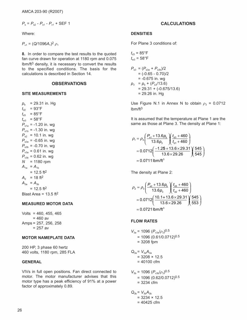
26
Ps = Ps2 - Ps1 - Pv1 + SEF 1
Where:
Pv1 = (Q/1096A1)2 ρ1
8. In order to compare the test results to the quoted
fan curve drawn for operation at 1180 rpm and 0.075
lbm/ft3 density, it is necessary to convert the results
to the specified conditions. The basis for the
calculations is described in Section 14.
OBSERVATIONS
SITE MEASUREMENTS
pb = 29.31 in. Hg
td2 = 93°F
td3 = 85°F
tw3 = 58°F
Ps1a = -1.20 in. wg
Ps1b = -1.30 in. wg
Ps2 = 10.1 in. wg
Ps3a = -0.65 in. wg
Ps3b = -0.70 in. wg
Pv3a = 0.61 in. wg
Pv3b = 0.62 in. wg
N = 1180 rpm
A1a = A1b
= 12.5 ft2
A2 = 18 ft2
A3a = A3b
= 12.5 ft2
Blast Area = 13.5 ft2
MEASURED MOTOR DATA
Volts = 460, 455, 465
= 460 av
Amps = 257, 256, 258
= 257 av
MOTOR NAMEPLATE DATA
200 HP, 3 phase 60 hertz
460 volts, 1180 rpm, 285 FLA
GENERAL
VIVs in full open positions. Fan direct connected to
motor. The motor manufacturer advises that this
motor type has a peak efficiency of 91% at a power
factor of approximately 0.89.
CALCULATIONS
DENSITIES
For Plane 3 conditions of:
td3 = 85°F
tw3 = 58°F
Ps3 = (Ps3a + Ps3b)/2
= (-0.65 - 0.70)/2
= -0.675 in. wg
p3 = pb + (Ps3/13.6)
= 29.31 + (-0.675/13.6)
= 29.26 in. Hg
Use Figure N.1 in Annex N to obtain ρ3 = 0.0712
lbm/ft3
It is assumed that the temperature at Plane 1 are the
same as those at Plane 3. The density at Plane 1:
The density at Plane 2:
FLOW RATES
V3a = 1096 (Pv3a/ρ3)0.5
= 1096 (0.61/0.0712)0.5
= 3208 fpm
Q3a = V3aA3a
= 3208 × 12.5
= 40100 cfm
V3b = 1096 (Pv3b/ρ3)0.5
= 1096 (0.62/0.0712)0.5
= 3234 cfm
Q3b = V3bA3b
= 3234 × 12.5
= 40425 cfm
ρ ρ2 3
13 6
13 6
460
460
0 071210 1
= +⎛
⎝⎜
⎞
⎠⎟
++
⎛
⎝⎜
⎞
⎠⎟
=
P pp
tt
s2 b
3
d3
d2
.
.
.. ++ ×
×⎛⎝⎜
⎞⎠⎟⎛⎝⎜
⎞⎠⎟
=
13 6 29 31
13 6 29 26
545
553
0 0721
. .
. .
. lbm/ft3
ρ ρ1 3
13 6
13 6
460
460
0 07121 2
= +⎛
⎝⎜
⎞
⎠⎟
++
⎛
⎝⎜
⎞
⎠⎟
= −
P pp
tt
s1 b
3
d3
d1
.
.
.. 55 13 6 29 31
13 6 29 26
545
545
0 0711
+ ××
⎛⎝⎜
⎞⎠⎟⎛⎝⎜
⎞⎠⎟
=
. .
. .
. lbm/ft3
AMCA 203-90 (R2007)

27
Q3 = Q3a + Q3b
= 40100 + 40425
= 80525 cfm
Q = Q1
= Q3 (ρ3/ρ1)
= 80525 (0.0712/0.0711)
= 80638 cfm
FAN POWER INPUT
Measured amps/FLA = (257/285)
= 0.90
= 90%
Annex K indicates that Equation A will provide a
reasonably accurate estimate of motor power output
for a 250 hp motor operating at 90% FLA.
Hmo = 250 (257/285) (460/460)
= 225 hp
As a check of this value, using the motor efficiency
data and the appropriate equation in Section 11.2.2:
Since the motor is not fully loaded, the power factor
and efficiency may be less, which would reduce Hmo
as calculated using the second method. However,
this is a reasonable check. The value of Hmo is
selected to be the average of the two results:
Hmo = 224 hp
Since the fan is direct-connected to the motor, there
is no drive loss, and:
H = Hmo
= 224 hp
SYSTEM EFFECT FACTOR
AMCA Publication 201-90, Figures 7.1 and 8.3
indicate the following calculations:
Q3 (ρ3/ρ2) = 80525 (0.0712/0.0721)
= 79520 cfm
(Q2/A2) = (79520/18)
= 4418 fpm
Blast area ratio = Blast Area/A2
= 13.5/18
= 0.75
For a blast area ratio of 0.75, and no duct, Figure 8.3
shows System Effect Curve T applies. For 4418 fpm
velocity and curve T, Figure 7.1 shows SEF 1 = 0.65
in. wg at 0.075 lbm/ft3. At 0.0720 lbm/ft3:
SEF 1 = 0.65 (0.0721/0.075)
= 0.62 in. wg
FAN STATIC PRESSURE
Pv1 = (Q1/1096 A1)2
= (80638/1096 × 25)2 0.0711
= 0.62 in. wg
Ps = Ps2 - Ps1 - Pv1 + SEF 1
= 10.1 - (-1.25) - 0.62 + 0.62
= 11.33 in. wg
CONVERSION TO SPECIFIED CONDITIONS
Qc = Q= 80638 cfm
Psc = 11.33 (0.075/0.0711)
= 11.95 in. wg
Hc = 224 (0.075/0.0711)
= 236 hp
Hmo
hp
= × × × ×
=
3 257 460 0 89 0 91
746
222
. .
AMCA 203-90 (R2007)
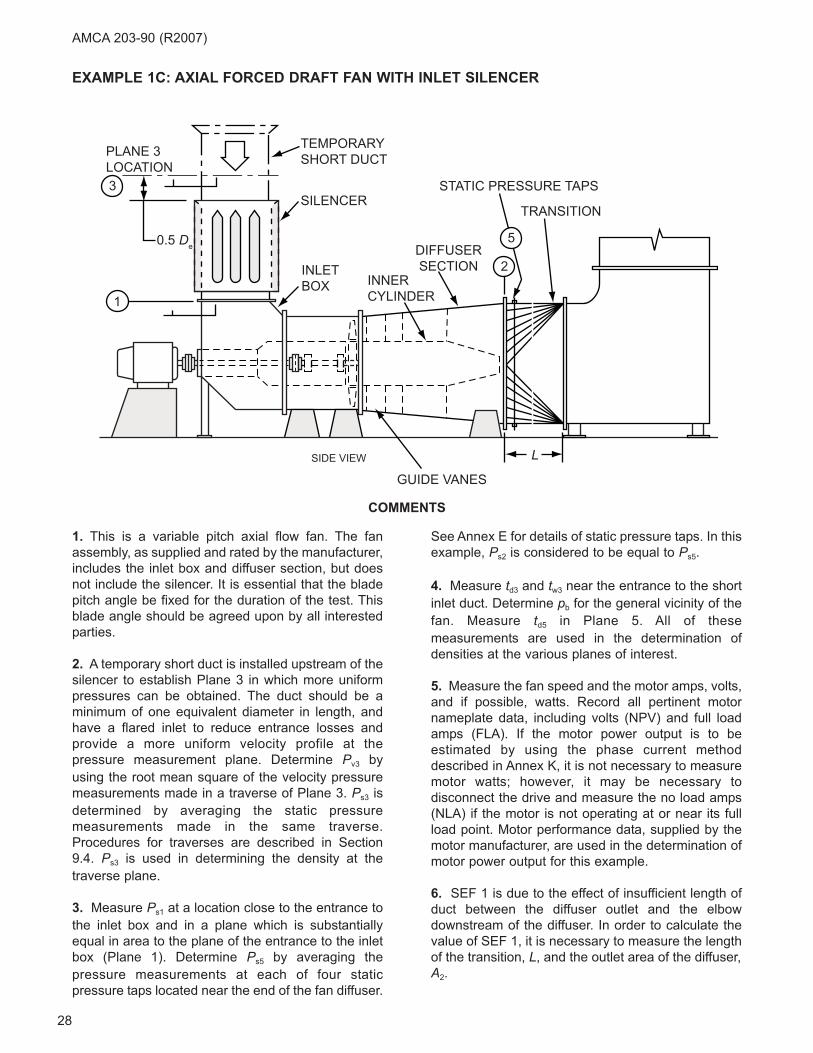
28
AMCA 203-90 (R2007)
1. This is a variable pitch axial flow fan. The fan
assembly, as supplied and rated by the manufacturer,
includes the inlet box and diffuser section, but does
not include the silencer. It is essential that the blade
pitch angle be fixed for the duration of the test. This
blade angle should be agreed upon by all interested
parties.
2. A temporary short duct is installed upstream of the
silencer to establish Plane 3 in which more uniform
pressures can be obtained. The duct should be a
minimum of one equivalent diameter in length, and
have a flared inlet to reduce entrance losses and
provide a more uniform velocity profile at the
pressure measurement plane. Determine Pv3 by
using the root mean square of the velocity pressure
measurements made in a traverse of Plane 3. Ps3 is
determined by averaging the static pressure
measurements made in the same traverse.
Procedures for traverses are described in Section
9.4. Ps3 is used in determining the density at the
traverse plane.
3. Measure Ps1 at a location close to the entrance to
the inlet box and in a plane which is substantially
equal in area to the plane of the entrance to the inlet
box (Plane 1). Determine Ps5 by averaging the
pressure measurements at each of four static
pressure taps located near the end of the fan diffuser.
See Annex E for details of static pressure taps. In this
example, Ps2 is considered to be equal to Ps5.
4. Measure td3 and tw3 near the entrance to the short
inlet duct. Determine pb for the general vicinity of the
fan. Measure td5 in Plane 5. All of these
measurements are used in the determination of
densities at the various planes of interest.
5. Measure the fan speed and the motor amps, volts,
and if possible, watts. Record all pertinent motor
nameplate data, including volts (NPV) and full load
amps (FLA). If the motor power output is to be
estimated by using the phase current method
described in Annex K, it is not necessary to measure
motor watts; however, it may be necessary to
disconnect the drive and measure the no load amps
(NLA) if the motor is not operating at or near its full
load point. Motor performance data, supplied by the
motor manufacturer, are used in the determination of
motor power output for this example.
6. SEF 1 is due to the effect of insufficient length of
duct between the diffuser outlet and the elbow
downstream of the diffuser. In order to calculate the
value of SEF 1, it is necessary to measure the length
of the transition, L, and the outlet area of the diffuser,
A2.
STATIC PRESSURE TAPS
TRANSITION
DIFFUSERSECTION
INNERCYLINDER
INLETBOX
SILENCER
TEMPORARYSHORT DUCT
GUIDE VANES
SIDE VIEW L
5
2
1
PLANE 3LOCATION3
0.5 De
EXAMPLE 1C: AXIAL FORCED DRAFT FAN WITH INLET SILENCER
COMMENTS
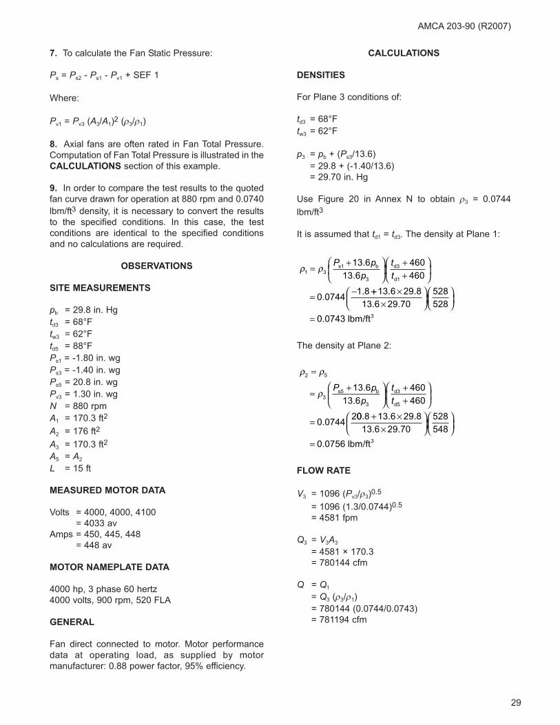
29
7. To calculate the Fan Static Pressure:
Ps = Ps2 - Ps1 - Pv1 + SEF 1
Where:
Pv1 = Pv3 (A3/A1)2 (ρ3/ρ1)
8. Axial fans are often rated in Fan Total Pressure.
Computation of Fan Total Pressure is illustrated in the
CALCULATIONS section of this example.
9. In order to compare the test results to the quoted
fan curve drawn for operation at 880 rpm and 0.0740
lbm/ft3 density, it is necessary to convert the results
to the specified conditions. In this case, the test
conditions are identical to the specified conditions
and no calculations are required.
OBSERVATIONS
SITE MEASUREMENTS
pb = 29.8 in. Hg
td3 = 68°F
tw3 = 62°F
td5 = 88°F
Ps1 = -1.80 in. wg
Ps3 = -1.40 in. wg
Ps5 = 20.8 in. wg
Pv3 = 1.30 in. wg
N = 880 rpm
A1 = 170.3 ft2
A2 = 176 ft2
A3 = 170.3 ft2
A5 = A2
L = 15 ft
MEASURED MOTOR DATA
Volts = 4000, 4000, 4100
= 4033 av
Amps = 450, 445, 448
= 448 av
MOTOR NAMEPLATE DATA
4000 hp, 3 phase 60 hertz
4000 volts, 900 rpm, 520 FLA
GENERAL
Fan direct connected to motor. Motor performance
data at operating load, as supplied by motor
manufacturer: 0.88 power factor, 95% efficiency.
CALCULATIONS
DENSITIES
For Plane 3 conditions of:
td3 = 68°F
tw3 = 62°F
p3 = pb + (Ps3/13.6)
= 29.8 + (-1.40/13.6)
= 29.70 in. Hg
Use Figure 20 in Annex N to obtain ρ3 = 0.0744
lbm/ft3
It is assumed that td1 = td3. The density at Plane 1:
The density at Plane 2:
FLOW RATE
V3 = 1096 (Pv3/ρ3)0.5
= 1096 (1.3/0.0744)0.5
= 4581 fpm
Q3 = V3A3
= 4581 × 170.3
= 780144 cfm
Q = Q1
= Q3 (ρ3/ρ1)
= 780144 (0.0744/0.0743)
= 781194 cfm
ρ ρ
ρ
2 5
3
13 6
13 6
460
460
0 07442
=
= +⎛
⎝⎜
⎞
⎠⎟
++
⎛
⎝⎜
⎞
⎠⎟
=
P pp
tt
s5 b
3
d3
d5
.
.
.00 8 13 6 29 8
13 6 29 70
528
548
0 0756
. . .
. .
.
+ ××
⎛⎝⎜
⎞⎠⎟⎛⎝⎜
⎞⎠⎟
= lbm/ft3
ρ ρ1 3
13 6
13 6
460
460
0 07441 8
= +⎛
⎝⎜
⎞
⎠⎟
++
⎛
⎝⎜
⎞
⎠⎟
= −
P pp
tt
s1 b
3
d3
d1
.
.
.. ++ ×
×⎛⎝⎜
⎞⎠⎟⎛⎝⎜
⎞⎠⎟
=
13 6 29 8
13 6 29 70
528
528
0 0743
. .
. .
. lbm/ft3
AMCA 203-90 (R2007)

30
FAN POWER INPUT
Since the fan is direct connected to the motor, there
is no drive loss, and:
H = Hmo
= 3507 hp
SYSTEM EFFECT FACTOR
AMCA Publication 201-90, Figures 7.1, 8.1, and 8.4
indicate the following calculations:
Q2 = Q3 (ρ3/ρ2)
= 780144 (0.0744/0.0756)
= 767761 cfm
V2 = (Q2/A2)
= (767761/176)
= 4362
Duct diameter equivalent to the diffuser outlet area:
Figure 8.1 shows that for velocities over 2500 fpm,
100% effective duct length is one duct diameter for
every 1000 fpm:
= De2 (V2/1000)
= 15 (4362/1000)
= 65.43 ft.
L in % effective duct length
= (L/65.43) 100
= (15/65.43) 100
= 23%
For 23% effective duct length and a vaneaxial fan
with a 2 piece elbow, Figure 8.4 shows System EffectCurve V applies. For 4362 fpm velocity and curve V,
Figure 7.1 shows SEF 1 = 0.32 in. wg at 0.075
lbm/ft3. At 0.0756 lbm/ft3.
SEF 1 = 0.32 (0.0756/0.075)
= 0.32 in. wg
FAN STATIC PRESSURE
Pv1 = Pv3 (A3/A1)2 (ρ3/ρ1)
= 1.3 (170.3/170.3)2 (0.0744/0.0743)
= 1.30 in. wg
Ps2 = Ps5
= 20.8 in. wg
Ps = Ps2 - Ps1 - Pv1 + SEF 1
= 20.8 - (-1.80) - 1.30 + 0.32
= 21.62 in. wg
FAN TOTAL PRESSURE
Pt1 = Ps1 +Pv1
= -1.8 + 1.30
= -0.50 in. wg
Pv2 = Pv3 (A3/A2)2 (ρ3/ρ2)
= 1.3 (170.3/176)2 (0.0744/0.0756)
= 1.20 in. wg
Pt2 = Ps2 + Pv2
= 20.8 + 1.20
= 22.00 in. wg
Pt = Pt2 - Pt1 + SEF 1
= 22.00 - (-0.50) + 0.32
= 22.82 in. wg
Also:
Pt = Ps + Pv
Pv = Pv2
= 1.20 in. wg
Pt = 21.62 + 1.20
= 22.82 in. wg
CONVERSION TO SPECIFIED CONDITIONS
Qc = Q= 781194 cfm
Psc = Ps
= 21.62 in. wg
Ptc = Pt
= 22.82 in. wg
Hc = H= 3507 hp
D Ae2
ft.
=
= ×( )=
4
4 176
15
2 /
/
π
π
Hmo
volts amps power factor efficiency= × × × ×
= × × ×
3
746
3 4033 448 0 8. 88 0 95
746
3507
×
=
.
hp
AMCA 203-90 (R2007)

31
AMCA 203-90 (R2007)
1. Each of the fans, as supplied and rated by the
manufacturer, includes an outlet damper.
Performance ratings for fans with outlet dampers
cover operation with the outlet damper in the full
open position. In order to be able to compare the test
results to the fan performance ratings it is essential
that the outlet dampers be fixed in the full open
positions for the duration of the test.
2. In this example, there are no suitable locations for
traverse planes for use in determining directly the
flow rate for each fan. The alternative is to determine
the total flow rate and since the fans and their
operating speeds are alike, assume that each fan
delivers a flow rate proportional to its actual speed.
Determine Pv3 by using the root mean square of the
velocity pressure measurements made in a traverse
of Plane 3, located near the end of a straight run of
duct, such as shown in the diagram. Determine Ps3 by
averaging the static pressure measurements made in
the same traverse. Procedures for traverses are
described in Section 9.4. Ps3 is used in determining
the density at the traverse plane. Measure the area of
traverse plane, A3, which is located at the tip of the
Pitot-static tube.
3. Determine Ps2 for each fan by averaging the
pressure measurements at each of four static
pressure taps located in the short length of duct
between the outlet damper and the plenum. See
Annex E for details of static pressure taps. Measure
td2 in Plane 2 for each fan.
4. For each fan, measure td1 and tw1 in the path of the
air flowing into the fan inlet. Determine pb for the
general vicinity of the fans. Measure td3 in Plane 3. All
of these measurements are used in the determination
of densities at the various planes of interest.
5. Measure the fan speed and the motor amps, volts,
and if possible, watts for each fan. Record all
pertinent motor nameplate data, including volts
(NPV) and full load amps (FLA). If the motor power
outputs are to be estimated by using the phase
current method described in Annex K, it is not
necessary to measure motor watts; however, it may
be necessary to disconnect the drives and measure
the no load amps (NLA) if the motors are not
operating at or near their full load points. Refer to
Annex K.
6. SEF 1 is due to the effect of insufficient length of
duct between the outlet of each fan and the plenum.
In this case, the duct length is so short as to be
judged equivalent to there being no duct at all. In
order to calculate the value of SEF 1, it is necessary
to measure the outlet areas of the fans, A2, and their
blast areas.
EXAMPLE 1D: CENTRIFUGAL FANS IN PARALLEL
1 1
2
3
STATIC PRESSURE TAPS
OUTLET DAMPER
SEF 1
PLENUM
SIDE VIEWPLAN VIEW
COMMENTS
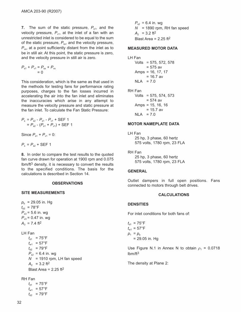
32
7. The sum of the static pressure, Ps1, and the
velocity pressure, Pv1, at the inlet of a fan with an
unrestricted inlet is considered to be equal to the sum
of the static pressure, Psx, and the velocity pressure,
Pvx, at a point sufficiently distant from the inlet as to
be in still air. At this point, the static pressure is zero,
and the velocity pressure in still air is zero.
Ps1 + Pv1 = Psx + Pvx
= 0
This consideration, which is the same as that used in
the methods for testing fans for performance rating
purposes, charges to the fan losses incurred in
accelerating the air into the fan inlet and eliminates
the inaccuracies which arise in any attempt to
measure the velocity pressure and static pressure at
the fan inlet. To calculate the Fan Static Pressure:
Ps = Ps2 - Ps1 - Pv1 + SEF 1
= Ps2 - (Ps1 + Pv1) + SEF 1
Since Ps1 + Pv1 = 0:
Ps = Ps2 + SEF 1
8. In order to compare the test results to the quoted
fan curve drawn for operation at 1900 rpm and 0.075
lbm/ft3 density, it is necessary to convert the results
to the specified conditions. The basis for the
calculations is described in Section 14.
OBSERVATIONS
SITE MEASUREMENTS
pb = 29.05 in. Hg
td3 = 78°F
Ps3 = 5.6 in. wg
Pv3 = 0.47 in. wg
A3 = 7.4 ft2
LH Fan
td1 = 75°F
tw1 = 57°F
td2 = 79°F
Ps2 = 6.4 in. wg
N = 1910 rpm, LH fan speed
A2 = 3.2 ft2
Blast Area = 2.25 ft2
RH Fan
td1 = 75°F
tw1 = 57°F
td2 = 79°F
Ps2 = 6.4 in. wg
N = 1890 rpm, RH fan speed
A2 = 3.2 ft2
Blast Area = 2.25 ft2
MEASURED MOTOR DATA
LH Fan
Volts = 575, 572, 578
= 575 av
Amps = 16, 17, 17
= 16.7 av
NLA = 7.0
RH Fan
Volts = 575, 574, 573
= 574 av
Amps = 15, 16, 16
= 15.7 av
NLA = 7.0
MOTOR NAMEPLATE DATA
LH Fan
25 hp, 3 phase, 60 hertz
575 volts, 1780 rpm, 23 FLA
RH Fan
25 hp, 3 phase, 60 hertz
575 volts, 1780 rpm, 23 FLA
GENERAL
Outlet dampers in full open positions. Fans
connected to motors through belt drives.
CALCULATIONS
DENSITIES
For inlet conditions for both fans of:
td1 = 75°F
tw1 = 57°F
p1 = pb
= 29.05 in. Hg
Use Figure N.1 in Annex N to obtain ρ1 = 0.0718
lbm/ft3
The density at Plane 2:
AMCA 203-90 (R2007)

33
The density at Plane 3:
FLOW RATES
V3 = 1096 (Pv3/ρ3)0.5
= 1096 (0.47/0.0724)0.5
= 2792 fpm
Q3 = V3A3
= 2792 × 7.4
= 20661 cfm
Q = Q1
= Q3 (ρ3/ρ1)
= 20661 (0.0724/0.0718)
= 20834 cfm
Assume that the air flow rate for each fan is
proportional to its speed.
LH Fan
Q = Q1
= 20834 [1910/(1910 + 1890)]
= 10472 cfm
RH Fan
Q = Q1
= 20834 [1890/(1910 + 1890)]
= 10362 cfm
FAN POWER INPUT
LH Fan
Measured amps/FLA = (16.7/23)
= 0.73
= 73%
RH Fan
Measured amps/FLA = (15.7/23)
= 0.68
= 68%
Annex K indicates that the average of the results of
Equation A and Equation B will provide a reasonably
accurate estimate of motor power output for a 25 hp
motor operating at approximately 70% FLA.
LH Fan
Eqn A = 25 (16.7/23) (575/575)
= 18.15 hp
Eqn B = 25 [(16.7 - 7)/(23 - 7)] (575/575)
= 15.16 hp
Hmo = (18.15 + 15.16)/2
= 16.66 hp
RH Fan
Eqn A = 25 (15.7/23) (574/575)
= 17.04 hp
Eqn B = 25 [(15.7 - 7)/(23 - 7)] (574/575)
= 13.57 hp
Hmo = (17.04 + 13.57)/2
= 15.31 hp
Figure L.1 in Annex L indicates estimated belt drive
loss of 5% for each fan.
LH Motor
HL = 0.05 Hmo
= 0.05 × 16.66
= 0.83 hp
H = Hmo - HL
= 16.66 - 0.83
= 15.83 hp
RH Motor
HL = 0.05 Hmo
= 0.05 × 15.31
= 0.77 hp
H = Hmo - HL
= 15.31 - 0.77
= 14.54 hp
SYSTEM EFFECT FACTOR
AMCA Publication 201-90, Figures 7.1 and 8.3
indicate the following calculations:
LH Fan
Q2 = Q1 (ρ1/ρ2)
= 10472 (0.0718/0.0724)
= 10385 cfm
V2 = (Q2/A2)
= (10385/3.2)
= 3245 fpm
ρ ρ2 1
1
13 6
13 6
460
460
0 07186 4
= +⎛
⎝⎜
⎞
⎠⎟
++
⎛
⎝⎜
⎞
⎠⎟
= +
P pp
tt
s2 b d1
d2
.
.
.. 113 6 29 05
13 6 29 05
535
539
0 0724 3
. .
. .
.
××
⎛⎝⎜
⎞⎠⎟⎛⎝⎜
⎞⎠⎟
= lbm/ft
ρ ρ3 1
1
13 6
13 6
460
460
0 07185 6
= +⎛
⎝⎜
⎞
⎠⎟
++
⎛
⎝⎜
⎞
⎠⎟
= +
P pp
tt
s3 b d1
d3
.
.
.. 113 6 29 05
13 6 29 05
535
538
0 0724 3
. .
. .
.
××
⎛⎝⎜
⎞⎠⎟⎛⎝⎜
⎞⎠⎟
= lbm/ft
AMCA 203-90 (R2007)

34
Blast area ratio = Blast Area/A2
= 2.25/3.2
= 0.70
RH Fan
Q2 = Q1 (ρ1/ρ2)
= 10362 (0.0718/0.0724)
= 10276 cfm
V2 = (Q2/A2)
= (10276/3.2)
= 3211 fpm
Blast area ratio = Blast Area/A2
= 2.25/3.2
= 0.70
For a blast area ratio of 0.7 and no duct, Figure 8.3
shows System Effect Curve S applies. For each fan
with velocities of 3245 fpm and 3211 fpm and curve
S, Figure 7.1 shows SEF 1 = 0.5 in. wg at 0.075
lbm/ft3. At 0.0724 lbm/ft3:
SEF 1 = 0.5 (0.0724/0.075)
= 0.48 in. wg
FAN STATIC PRESSURE
Ps = Ps2 + SEF 1
LH Fan
Ps = 6.4 + 0.48
= 6.88 in. wg
RH Fan
Ps = 6.4 + 0.48
= 6.88 in. wg
CONVERSION TO SPECIFIED CONDITIONS
LH Fan
Qc = 10472 (1900/1910)
= 10417 cfm
Psc = 6.88 (1900/1910)2 (0.075/0.0718)
= 7.11 in. wg
Hc = 15.83 (1900/1910)3 (0.075/0.0718)
= 16.28 hp
RH Fan
Qc = 10362 (1900/1890)
= 10417 cfm
Psc = 6.88 (1900/1890)2 (0.075/0.0718)
= 7.26 in. wg
Hc = 14.54 (1900/1890)3 (0.075/0.0718)
= 15.43 hp
AMCA 203-90 (R2007)
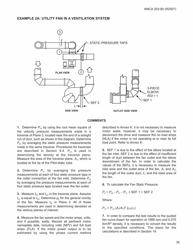
35
AMCA 203-90 (R2007)
1. Determine Pv3 by using the root mean square of
the velocity pressure measurements made in a
traverse of Plane 3, located near the end of a straight
run of duct, such as shown in the diagram. Determine
Ps3 by averaging the static pressure measurements
made in the same traverse. Procedures for traverses
are described in Section 9.4. Ps3 is used in
determining the density at the traverse plane.
Measure the area of the traverse plane, A3, which is
located at the tip of the Pitot-static tube.
2. Determine Ps1 by averaging the pressure
measurements at each of four static pressure taps in
the collar connection at the fan inlet. Determine Ps2
by averaging the pressure measurements at each of
four static pressure taps located near the fan outlet.
3. Measure td3 and tw3 in the traverse plane. Assume
td1 is equal to td3. Determine pb for the general vicinity
of the fan. Measure td2 in Plane 2. All of these
measurements are used in determining densities at
the various planes of interest.
4. Measure the fan speed and the motor amps, volts,
and if possible, watts. Record all pertinent motor
nameplate data, including volts (NPV) and full load
amps (FLA). If the motor power output is to be
estimated by using the phase current method
described in Annex K, it is not necessary to measure
motor watts; however, it may be necessary to
disconnect the drive and measure the no load amps
(NLA) if the motor is not operating at or near its full
load point. Refer to Annex K.
5. SEF 1 is due to the effect of the elbow located at
the fan inlet. SEF 2 is due to the effect of insufficient
length of duct between the fan outlet and the elbow
downstream of the fan. In order to calculate the
values of the SEFs, it is necessary to measure the
inlet area and the outlet area of the fan, A1 and A2;
the length of the outlet duct, L; and the blast area of
the fan.
6. To calculate the Fan Static Pressure:
Ps = Ps2 - Ps1 - Pv1 + SEF 1 + SEF 2
Where:
Pv1 = Pv3 (A3/A1)2 (ρ3/ρ1)
7. In order to compare the test results to the quoted
fan curve drawn for operation at 1880 rpm and 0.075
lbm/ft3 density, it is necessary to convert the results
to the specified conditions. The basis for the
calculations is described in Section 14.
EXAMPLE 2A: UTILITY FAN IN A VENTILATION SYSTEM
SIDE VIEW OUTLET SIDE VIEW
PLAN VIEW
STATIC PRESSURE TAPS
SEF 2L
3
1
2
3-PIECEELBOWR/D = 1
SEF 1
COMMENTS
36
OBSERVATIONS
SITE MEASUREMENTS
pb = 29.20 in. Hg
td2 = 72°F
td3 = 72°F
tw3 = 66°F
Ps1 = -2.18 in. wg
Ps2 = 0.35 in. wg
Ps3 = -1.95 in. wg
Pv3 = 0.45 in. wg
N = 1730 rpm
A1 = 1.07 ft2
A2 = 1.17 ft2
A3 = 1.07 ft2
Blast Area = 0.7 ft2
L = 0.83 ft
MEASURED MOTOR DATA
Volts = 227, 229, 228
= 228 av
Amps = 10.2, 10.3, 10.4
= 10.3 av
NLA = 7.1
MOTOR NAMEPLATE DATA
5 hp, 3 phase, 60 hertz
230 volts, 1750 rpm, 14 FLA
GENERAL
Fan connected to motor through belt drive.
CALCULATIONS
DENSITIES
For Plane 3 conditions of:
td3 = 72°F
tw3 = 66°F
p3 = pb + (Ps3/13.6)
= 29.20 + (-1.95/13.6)
= 29.06 in. Hg
Use Figure N.1 in Annex N to obtain ρ3 = 0.0719
lbm/ft3
It is assumed that td1 = td3
The density at Plane 1:
The density at Plane 2:
FLOW RATES
V3 = 1096 (Pv3/ρ3)0.5
= 1096 (0.45/0.0719)0.5
= 2742 fpm
Q3 = V3A3
= 2742 × 1.07
= 2934 cfm
Q = Q1
= Q3 (ρ3/ρ1)
= 2934 (0.0719/0.0718)
= 2938 cfm
FAN POWER INPUT
Measured amps/FLA = 10.3/14
= 0.74
= 74%
Annex K indicates that the average of the results of
Equation A and Equation B will provide a reasonably
accurate estimate of motor power output for a 5 hp
motor operating at 74% FLA.
Eqn A = 5 (10.3/14) (228/230)
= 3.65 hp
Eqn B = 5 [(10.3 - 7.1)/(14 - 7.1)] (228/230)
= 2.30 hp
Hmo = (3.65 + 2.30)/2
= 2.98 hp
ρ ρ2 3
3
13 6
13 6
460
460
0 07190 35
= +⎛
⎝⎜
⎞
⎠⎟
++
⎛
⎝⎜
⎞
⎠⎟
=
P pp
tt
s2 b d3
d2
.
.
.. ++ ×
×⎛⎝⎜
⎞⎠⎟⎛⎝⎜
⎞⎠⎟
=
13 6 29 20
13 6 29 06
532
532
0 0723 3
. .
. .
. lbm/ft
ρ ρ1 3
3
13 6
13 6
460
460
0 07192 1
= +⎛
⎝⎜
⎞
⎠⎟
++
⎛
⎝⎜
⎞
⎠⎟
= −
P pp
tt
s1 b d3
d1
.
.
.. 88 13 6 29 20
13 6 29 06
532
532
0 0718 3
+ ××
⎛⎝⎜
⎞⎠⎟⎛⎝⎜
⎞⎠⎟
=
. .
. .
. lbm/ft
AMCA 203-90 (R2007)
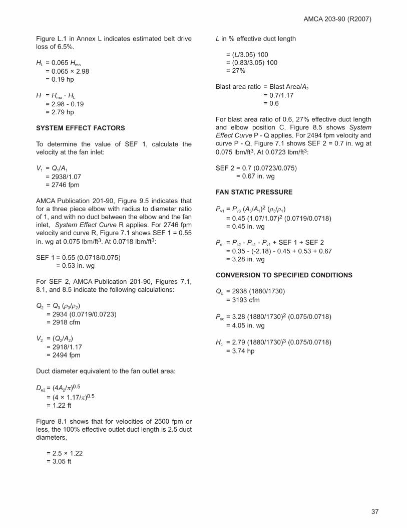
37
Figure L.1 in Annex L indicates estimated belt drive
loss of 6.5%.
HL = 0.065 Hmo
= 0.065 × 2.98
= 0.19 hp
H = Hmo - HL
= 2.98 - 0.19
= 2.79 hp
SYSTEM EFFECT FACTORS
To determine the value of SEF 1, calculate the
velocity at the fan inlet:
V1 = Q1/A1
= 2938/1.07
= 2746 fpm
AMCA Publication 201-90, Figure 9.5 indicates that
for a three piece elbow with radius to diameter ratio
of 1, and with no duct between the elbow and the fan
inlet, System Effect Curve R applies. For 2746 fpm
velocity and curve R, Figure 7.1 shows SEF 1 = 0.55
in. wg at 0.075 lbm/ft3. At 0.0718 lbm/ft3:
SEF 1 = 0.55 (0.0718/0.075)
= 0.53 in. wg
For SEF 2, AMCA Publication 201-90, Figures 7.1,
8.1, and 8.5 indicate the following calculations:
Q2 = Q3 (ρ3/ρ2)
= 2934 (0.0719/0.0723)
= 2918 cfm
V2 = (Q2/A2)
= 2918/1.17
= 2494 fpm
Duct diameter equivalent to the fan outlet area:
De2 = (4A2/π)0.5
= (4 × 1.17/π)0.5
= 1.22 ft
Figure 8.1 shows that for velocities of 2500 fpm or
less, the 100% effective outlet duct length is 2.5 duct
diameters,
= 2.5 × 1.22
= 3.05 ft
L in % effective duct length
= (L/3.05) 100
= (0.83/3.05) 100
= 27%
Blast area ratio = Blast Area/A2
= 0.7/1.17
= 0.6
For blast area ratio of 0.6, 27% effective duct length
and elbow position C, Figure 8.5 shows SystemEffect Curve P - Q applies. For 2494 fpm velocity and
curve P - Q, Figure 7.1 shows SEF 2 = 0.7 in. wg at
0.075 lbm/ft3. At 0.0723 lbm/ft3:
SEF 2 = 0.7 (0.0723/0.075)
= 0.67 in. wg
FAN STATIC PRESSURE
Pv1 = Pv3 (A3/A1)2 (ρ3/ρ1)
= 0.45 (1.07/1.07)2 (0.0719/0.0718)
= 0.45 in. wg
Ps = Ps2 - Ps1 - Pv1 + SEF 1 + SEF 2
= 0.35 - (-2.18) - 0.45 + 0.53 + 0.67
= 3.28 in. wg
CONVERSION TO SPECIFIED CONDITIONS
Qc = 2938 (1880/1730)
= 3193 cfm
Psc = 3.28 (1880/1730)2 (0.075/0.0718)
= 4.05 in. wg
Hc = 2.79 (1880/1730)3 (0.075/0.0718)
= 3.74 hp
AMCA 203-90 (R2007)
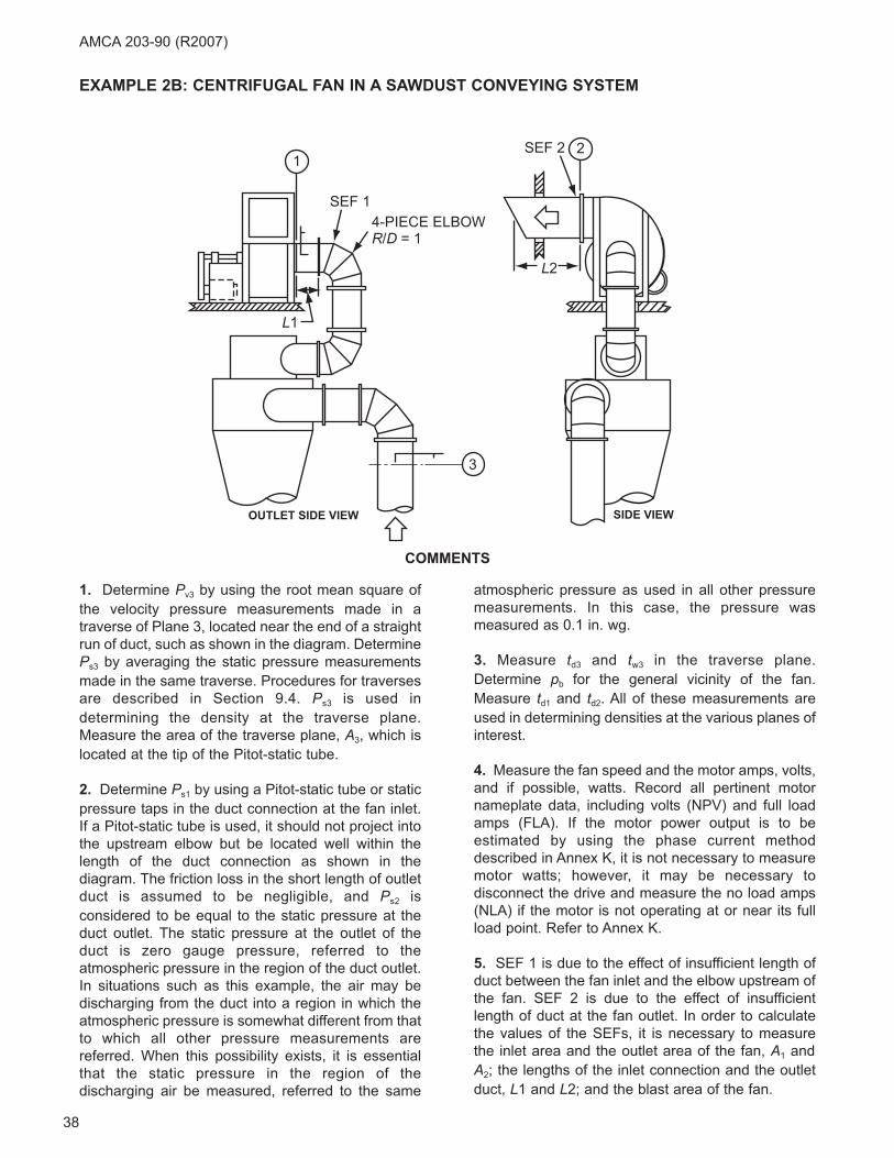
38
AMCA 203-90 (R2007)
1. Determine Pv3 by using the root mean square of
the velocity pressure measurements made in a
traverse of Plane 3, located near the end of a straight
run of duct, such as shown in the diagram. Determine
Ps3 by averaging the static pressure measurements
made in the same traverse. Procedures for traverses
are described in Section 9.4. Ps3 is used in
determining the density at the traverse plane.
Measure the area of the traverse plane, A3, which is
located at the tip of the Pitot-static tube.
2. Determine Ps1 by using a Pitot-static tube or static
pressure taps in the duct connection at the fan inlet.
If a Pitot-static tube is used, it should not project into
the upstream elbow but be located well within the
length of the duct connection as shown in the
diagram. The friction loss in the short length of outlet
duct is assumed to be negligible, and Ps2 is
considered to be equal to the static pressure at the
duct outlet. The static pressure at the outlet of the
duct is zero gauge pressure, referred to the
atmospheric pressure in the region of the duct outlet.
In situations such as this example, the air may be
discharging from the duct into a region in which the
atmospheric pressure is somewhat different from that
to which all other pressure measurements are
referred. When this possibility exists, it is essential
that the static pressure in the region of the
discharging air be measured, referred to the same
atmospheric pressure as used in all other pressure
measurements. In this case, the pressure was
measured as 0.1 in. wg.
3. Measure td3 and tw3 in the traverse plane.
Determine pb for the general vicinity of the fan.
Measure td1 and td2. All of these measurements are
used in determining densities at the various planes of
interest.
4. Measure the fan speed and the motor amps, volts,
and if possible, watts. Record all pertinent motor
nameplate data, including volts (NPV) and full load
amps (FLA). If the motor power output is to be
estimated by using the phase current method
described in Annex K, it is not necessary to measure
motor watts; however, it may be necessary to
disconnect the drive and measure the no load amps
(NLA) if the motor is not operating at or near its full
load point. Refer to Annex K.
5. SEF 1 is due to the effect of insufficient length of
duct between the fan inlet and the elbow upstream of
the fan. SEF 2 is due to the effect of insufficient
length of duct at the fan outlet. In order to calculate
the values of the SEFs, it is necessary to measure
the inlet area and the outlet area of the fan, A1 and
A2; the lengths of the inlet connection and the outlet
duct, L1 and L2; and the blast area of the fan.
EXAMPLE 2B: CENTRIFUGAL FAN IN A SAWDUST CONVEYING SYSTEM
3
12SEF 2
4-PIECE ELBOWR/D = 1
SEF 1
SIDE VIEWOUTLET SIDE VIEW
L1
L2
COMMENTS
39
6. To calculate the Fan Static Pressure:
Ps = Ps2 - Ps1 - Pv1 + SEF 1 + SEF 2
Where:
Pv1 = Pv3 (A3/A1)2 (ρ3/ρ1)
7. In order to compare the test results to the quoted
fan curve drawn for operation at 2075 rpm and 0.075
lbm/ft3, it is necessary to convert the results to the
specified conditions. The basis for the calculations is
described in Section 14.
OBSERVATIONS
SITE MEASUREMENTS
pb = 29.82 in. Hg
td1 = 86.6°F
td2 = 91.3°F
tw2 = 70.4°F
td3 = 86°F
Ps1 = -11.4 in. wg
Ps2 = 0.1 in. wg
Ps3 = -8.9 in. wg
Pv3 = 1.24 in. wg
N = 2120 rpm, fan speed
A1 = 1.40 ft2
A2 = 1.40 ft2
A3 = 1.57 ft2
Blast Area = 1.26 ft2
L1 = 1.33 ft
L2 = 3.0 ft
MEASURED MOTOR DATA
Volts = 460, 460, 459
= 460 av
Amps = 26.5, 25.5, 26
= 26 av
NLA = 11.3
MOTOR NAMEPLATE DATA
30 hp, 3 phase, 60 hertz
460 volts, 1750 rpm, 36 FLA
GENERAL
Fan connected to motor through belt drive.
CALCULATION
DENSITIES
For Plane 2 conditions of:
td2 = 91.3°F
tw2 = 70.4°F
p2 = pb + (Ps2/13.6)
= 29.82 + (0.1/13.6)
= 29.83 in. Hg
Use Figure N.1 in Annex N to obtain ρ2 = 0.0714
lbm/ft3
The density at Plane 1:
The density at Plane 3:
FLOW RATES
V3 = 1096 (Pv3/ρ3)0.5
= 1096 (1.24/0.0705)0.5
= 4596 fpm
Q3 = V3A3
= 4596 × 1.57
= 7216 cfm
Q = Q1
= Q3 (ρ3/ρ1)
= 7216 (0.0705/0.0700)
= 7268 cfm
FAN POWER INPUT
Measured amps/FLA = (26/36)
= 0.72
= 72%
ρ ρ3 2
3
13 6
13 6
460
460
0 07148 9
= +⎛
⎝⎜
⎞
⎠⎟
++
⎛
⎝⎜
⎞
⎠⎟
= −
P pp
tt
s3 b d2
d3
.
.
.. ++ ×
×⎛⎝⎜
⎞⎠⎟⎛⎝⎜
⎞⎠⎟
=
13 6 29 82
13 6 29 83
551 3
546
0 0705
. .
. .
.
. lbm/ft3
ρ ρ1 2
2
13 6
13 6
460
460
0 071411
= +⎛
⎝⎜
⎞
⎠⎟
++
⎛
⎝⎜
⎞
⎠⎟
= −
P pp
tt
s1 b d2
d1
.
.
..44 13 6 29 82
13 6 29 83
551 3
546 6
0 0700
+ ××
⎛⎝⎜
⎞⎠⎟⎛⎝⎜
⎞⎠⎟
=
. .
. .
.
.
. lbm/ft33
AMCA 203-90 (R2007)
40
Annex K indicates that the average of the results of
Equation A and Equation B will provide a reasonably
accurate estimate of motor power output for a 30 hp
motor operating at 72% FLA.
Eqn A = 30 (26/36) (460/460)
= 21.67 hp
Eqn B = 30 [(26 - 11.3)/(36 - 11.3)] (460/460)
= 17.85 hp
Hmo = (21.67 + 17.85)/2
= 19.76 hp
Figure L.1 in Annex L indicates estimated belt drive
loss of 4.8%.
HL = 0.048 Hmo
= 0.048 × 19.76
= 0.95 hp
H = Hmo - HL
= 19.76 - 0.95
= 18.81 hp
SYSTEM EFFECT FACTORS
To determine the value of SEF 1, calculate the
velocity at the fan inlet:
V1 = (Q1/A1)
= (7268/1.40)
= 5191 fpm
The diameter of the fan inlet:
D1 = (4A1/π)0.5
= (4 × 1.40/π)0.5
= 1.34 ft.
The length of the duct between the elbow and the fan
inlet in terms of D1:
= (L1/D1)
= (1.33/1.34)
= 1.0
AMCA Publication 201-90, Figure 9.5 indicates that
for a four piece elbow with a radius to diameter ratio
of 1, and with a length of duct between the elbow and
the fan inlet equal to 1 equivalent diameter, SystemEffect Curve S applies. For 5191 fpm velocity and
curve S, Figure 7.1 shows SEF 1 = 1.3 in. wg at
0.075 lbm/ft3. At 0.0700 lbm/ft3:
SEF 1 = 1.3 (0.0700/0.075)
= 1.2 in. wg
For SEF 2, AMCA Publication 201-90, Figure 8.3
indicates the following calculations:
Q2 = Q3 (ρ3/ρ2)
= 7216 (0.0705/0.0714)
= 7125 cfm
V2 = (Q2/A2)
= (7125/1.40)
= 5089 fpm
Duct diameter equivalent to the fan outlet area:
De2 = (4A2/π)0.5
= (4 × 1.40/π)0.5
= 1.34 ft
Figure 8.3 shows that for velocities over 2500 fpm,
100% effective duct length is one duct diameter per
1000 fpm:
= D2 (V2/1000)
= 1.34 (5089/1000)
= 6.82 ft
The length of the outlet duct in % effective duct
length:
= (L2/6.82) 100
= (3.0/6.82) 100
= 44%
Blast ratio area = Blast Area/A2
= 1.26/1.40
= 0.9
For blast area ratio of 0.9 and 44% effective duct
length, Figure 8.3 shows no System Effect Curveapplies and SEF 2 = 0.
FAN STATIC PRESSURE
Pv1 = Pv3 (A3/A1)2 (ρ3/ρ1)
= 1.24 (1.57/1.40)2 (0.0705/0.0700)
= 1.57 in. wg
Ps = Ps2 - Ps1 - Pv1 + SEF 1 + SEF 2
= 0.1 - (-11.4) - 1.57 + 1.2 + 0
= 11.13 in. wg
CONVERSIONS TO SPECIFIED CONDITIONS
Qc = 7268 (2075/2120)
= 7114 cfm
Psc = 11.13 (2075/2120)2 (0.075/0.0700)
= 11.42 in. wg
AMCA 203-90 (R2007)
41
Hc = 18.81 (2075/2120)2 (0.075/0.0700)
= 18.90 hp
AMCA 203-90 (R2007)
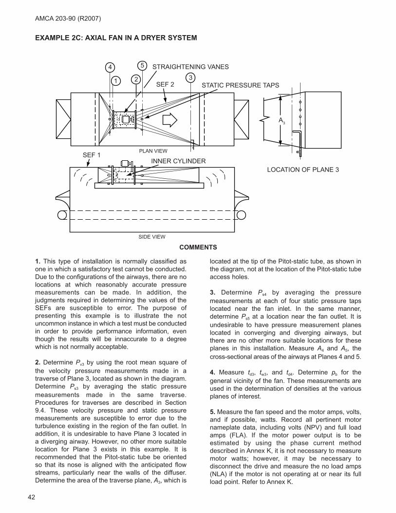
42
AMCA 203-90 (R2007)
1. This type of installation is normally classified as
one in which a satisfactory test cannot be conducted.
Due to the configurations of the airways, there are no
locations at which reasonably accurate pressure
measurements can be made. In addition, the
judgments required in determining the values of the
SEFs are susceptible to error. The purpose of
presenting this example is to illustrate the not
uncommon instance in which a test must be conducted
in order to provide performance information, even
though the results will be innaccurate to a degree
which is not normally acceptable.
2. Determine Pv3 by using the root mean square of
the velocity pressure measurements made in a
traverse of Plane 3, located as shown in the diagram.
Determine Ps3 by averaging the static pressure
measurements made in the same traverse.
Procedures for traverses are described in Section
9.4. These velocity pressure and static pressure
measurements are susceptible to error due to the
turbulence existing in the region of the fan outlet. In
addition, it is undesirable to have Plane 3 located in
a diverging airway. However, no other more suitable
location for Plane 3 exists in this example. It is
recommended that the Pitot-static tube be oriented
so that its nose is aligned with the anticipated flow
streams, particularly near the walls of the diffuser.
Determine the area of the traverse plane, A3, which is
located at the tip of the Pitot-static tube, as shown in
the diagram, not at the location of the Pitot-static tube
access holes.
3. Determine Ps4 by averaging the pressure
measurements at each of four static pressure taps
located near the fan inlet. In the same manner,
determine Ps5 at a location near the fan outlet. It is
undesirable to have pressure measurement planes
located in converging and diverging airways, but
there are no other more suitable locations for these
planes in this installation. Measure A4 and A5, the
cross-sectional areas of the airways at Planes 4 and 5.
4. Measure td3, tw3, and td4. Determine pb for the
general vicinity of the fan. These measurements are
used in the determination of densities at the various
planes of interest.
5. Measure the fan speed and the motor amps, volts,
and if possible, watts. Record all pertinent motor
nameplate data, including volts (NPV) and full load
amps (FLA). If the motor power output is to be
estimated by using the phase current method
described in Annex K, it is not necessary to measure
motor watts; however, it may be necessary to
disconnect the drive and measure the no load amps
(NLA) if the motor is not operating at or near its full
load point. Refer to Annex K.
EXAMPLE 2C: AXIAL FAN IN A DRYER SYSTEM
COMMENTS
4 5
1 2
STRAIGHTENING VANES
STATIC PRESSURE TAPS3
SEF 2
A3
SEF 1INNER CYLINDER
PLAN VIEW
SIDE VIEW
LOCATION OF PLANE 3

43
6. Although an elbow is located a short distance
upstream of the fan, it is considered to produce no
system effect since it is equipped with turning vanes
and the average velocity through the elbow will be
relatively low due to its large cross-sectional area.
Therefore, SEF 1 = 0. In judging SEF 2, the rapidly
diverging transition fitting downstream of the fan is
considered equivalent to no duct at the fan outlet. In
order to calculate the value of SEF2, it is necessary
to measure the outlet area of the fan, A2.
7. To calculate the Fan Static Pressure,
Ps = Ps2 - Ps1 - Pv1 + SEF 1 + SEF 2
Where:
Pv1 = Pv3 (A3/A1)2 (ρ3/ρ1)
Ps1 and Ps2 are calculated on the basis of total
pressure considerations, using Ps4, Ps5, and the
calculated velocity pressures at Planes 1, 2, 4, and 5.
8. In order to compare the test results to the quoted
fan curve drawn for operation at 1580 rpm and
0.0690 lbm/ft3 density, it is necessary to convert the
results to the specified conditions. The basis for the
calculations is described in Section 14.
OBSERVATIONS
SITE MEASUREMENTS
pb = 28.90 in. Hg
td3 = 86.5°F
tw3 = 75.5°F
td4 = 85°F
Ps3 = 1.5 in. wg
Pv3 = 0.044 in. wg
Ps4 = -1.57 in. wg
Ps5 = 1.22 in. wg
N = 1590 rpm
A1 = A2 = 8.0 ft2
A3 = 29.8 ft2
A4 = 12.4 ft2
A5 = 9.6 ft2
MEASURED MOTOR DATA
Volts = 450, 449, 448
= 449 av
Amps = 25.0, 24.5, 25.0
= 24.8 av
NLA = 9.4
MOTOR NAMEPLATE DATA
25 hp, 3 phase, 60 hertz
460 volts, 1750 rpm, 31 FLA
GENERAL
Fan connected to motor through belt drive
CALCULATIONS
DENSITIES
For Plane 3 conditions of:
td3 = 86.5°F
tw3 = 75.5°F
p3 = pb + (Ps3/13.6)
= 28.90 + (1.5/13.6)
= 29.01 in. Hg
Use Figure N.1 from Annex N to obtain ρ3 = 0.0694
lbm/ft3
The density at Plane 4:
It is assumed that td1 = td4 and at the low pressure
levels which exist at Planes 1 and 4, the difference
between these pressures will be small, and assuming
ρ1 = ρ4, will result in an error which is considered
negligible. By similar reasoning, it is assumed that
ρ5 = ρ2 = ρ3.
FLOW RATES
V3 = 1096 (Pv3/ρ3)0.5
= 1096 (0.044/0.0694)0.5
= 873 fpm
Q3 = V3A3
= 873 × 29.8
= 26015 cfm
Q = Q1
= Q3 (ρ3/ρ1)
= 26015 (0.0694/0.0691)
= 26128 cfm
ρ ρ4 3
3
13 6
13 6
460
460
0 06941 5
= +⎛
⎝⎜
⎞
⎠⎟
++
⎛
⎝⎜
⎞
⎠⎟
= −
P pp
tt
s4 b d3
d4
.
.
.. 77 13 6 28 90
13 6 29 01
546 5
545
0 0691
+ ××
⎛⎝⎜
⎞⎠⎟⎛⎝⎜
⎞⎠⎟
=
. .
. .
.
. lbm/ft3
AMCA 203-90 (R2007)

44
FAN POWER INPUT
Measured amps/FLA = (24.8/31)
= 0.80
= 80%
Annex K indicates that the average of the results of
Equation A and Equation B will provide a reasonably
accurate estimate of motor power output for a 25 hp
motor operating at 80% FLA.
Eqn A = 25 (24.8/31) (449/460)
= 19.52 hp
Eqn B = 25 [(24.8 - 9.4)/(31 - 9.4)] (449/460)
= 17.40 hp
Hmo = (19.52 + 17.40)/2
= 18.46 hp
Figure L.1 in Annex L indicates estimated belt drive
loss of 4.9%.
HL = 0.049 Hmo
= 0.049 × 18.46
= 0.90 hp
H = Hmo - HL
= 18.46 - 0.90
= 17.56 hp
SYSTEM EFFECT FACTORS
SEF 1 = 0 See item 6 under COMMENTS.
To determine the value of SEF 2, AMCA Publication
201-90, Figure 8.2 indicates that a vaneaxial fan with
no outlet duct will use System Effect Curve U.
Q2 = Q3 (ρ3/ρ2)
= 26015 (0.0694/0.0694)
= 26015 cfm
V2 = (Q2/A2)
= (26015/8.0)
= 3252 fpm
From Figure 7.1, using 3252 fpm and curve U, SEF 2
= 0.26 in. wg at 0.075 lbm/ft3. At 0.0694 lbm/ft3:
SEF 2 = 0.26 (0.0694/0.075)
= 0.24 in. wg
FAN STATIC PRESSURE
Pv4 = Pv3 (A3/A4)2 (ρ3/ρ4)
= 0.044 (29.8/12.4)2 (0.0694/0.0691)
= 0.26 in. wg
Pv1 = Pv3 (A3/A1)2 (ρ3/ρ1)
= 0.044 (29.8/8.0)2 (0.0694/0.0691)
= 0.61 in. wg
Ps1 + Pv1 = Ps4 + Pv4
Ps1 = Ps4 + Pv4 - Pv1
= -1.57 + 0.26 - 0.61
= -1.92 in. wg
Pv5 = Pv3 (A3/A5)2 (ρ3/ρ5)
= 0.044 (29.8/9.6)2 (0.0694/0.0694)
= 0.42 in. wg
Pv2 = Pv3 (A3/A2)2 (ρ3/ρ2)
= 0.044 (29.8/8.0)2 (0.0694/0.0694)
= 0.61 in. wg
Ps2 + Pv2 = Ps5 + Pv5
Ps2 = Ps5 + Pv5 - Pv2
= 1.22 + 0.42 - 0.61
= 1.03 in. wg
Ps = Ps2 - Ps1 - Pv1 + SEF 1 + SEF 2
= 1.03 - (-1.92) - 0.61 + 0 + 0.24
= 2.58 in. wg
Losses between Planes 1 and 4 and between Planes
2 and 5 have been ignored.
CONVERSION TO SPECIFIED CONDITIONS
Qc = 26128 (1580/1590)
= 25964 cfm
Psc = 2.58 (1580/1590)2 (0.0690/0.0691)
= 2.54 in. wg
Hc = 17.56 (1580/1590)3 (0.0690/0.0691)
= 17.21 hp
AMCA 203-90 (R2007)
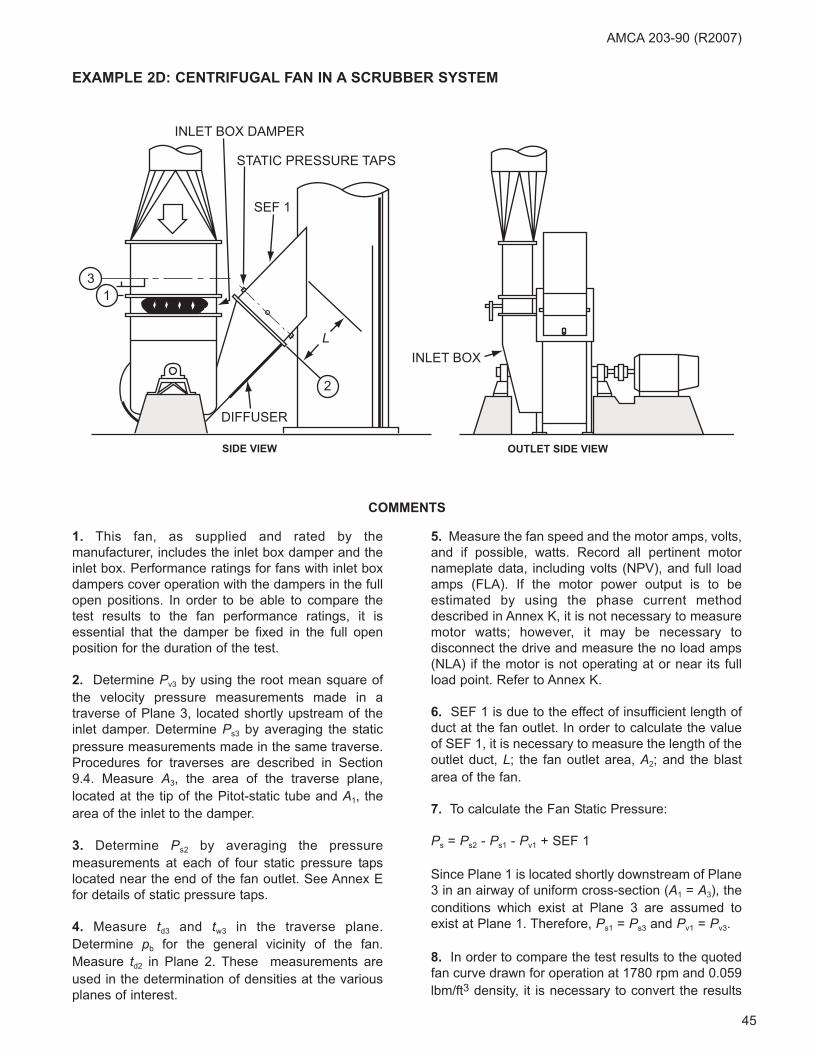
45
AMCA 203-90 (R2007)
1. This fan, as supplied and rated by the
manufacturer, includes the inlet box damper and the
inlet box. Performance ratings for fans with inlet box
dampers cover operation with the dampers in the full
open positions. In order to be able to compare the
test results to the fan performance ratings, it is
essential that the damper be fixed in the full open
position for the duration of the test.
2. Determine Pv3 by using the root mean square of
the velocity pressure measurements made in a
traverse of Plane 3, located shortly upstream of the
inlet damper. Determine Ps3 by averaging the static
pressure measurements made in the same traverse.
Procedures for traverses are described in Section
9.4. Measure A3, the area of the traverse plane,
located at the tip of the Pitot-static tube and A1, the
area of the inlet to the damper.
3. Determine Ps2 by averaging the pressure
measurements at each of four static pressure taps
located near the end of the fan outlet. See Annex E
for details of static pressure taps.
4. Measure td3 and tw3 in the traverse plane.
Determine pb for the general vicinity of the fan.
Measure td2 in Plane 2. These measurements are
used in the determination of densities at the various
planes of interest.
5. Measure the fan speed and the motor amps, volts,
and if possible, watts. Record all pertinent motor
nameplate data, including volts (NPV), and full load
amps (FLA). If the motor power output is to be
estimated by using the phase current method
described in Annex K, it is not necessary to measure
motor watts; however, it may be necessary to
disconnect the drive and measure the no load amps
(NLA) if the motor is not operating at or near its full
load point. Refer to Annex K.
6. SEF 1 is due to the effect of insufficient length of
duct at the fan outlet. In order to calculate the value
of SEF 1, it is necessary to measure the length of the
outlet duct, L; the fan outlet area, A2; and the blast
area of the fan.
7. To calculate the Fan Static Pressure:
Ps = Ps2 - Ps1 - Pv1 + SEF 1
Since Plane 1 is located shortly downstream of Plane
3 in an airway of uniform cross-section (A1 = A3), the
conditions which exist at Plane 3 are assumed to
exist at Plane 1. Therefore, Ps1 = Ps3 and Pv1 = Pv3.
8. In order to compare the test results to the quoted
fan curve drawn for operation at 1780 rpm and 0.059
lbm/ft3 density, it is necessary to convert the results
EXAMPLE 2D: CENTRIFUGAL FAN IN A SCRUBBER SYSTEM
COMMENTS
INLET BOX
OUTLET SIDE VIEWSIDE VIEW
INLET BOX DAMPER
STATIC PRESSURE TAPS
DIFFUSER
SEF 1
31
2
L
46
to the specified conditions. The basis for the
calculations is described in Section 14.
OBSERVATIONS
SITE MEASUREMENTS
pb = 29.44 in. Hg
td2 = 97°F
td3 = 63°F
tw3 = 62°F
Ps2 = 1.1 in. wg
Ps3 = -70.2 in. wg
Pv3 = 0.64 in. wg
N = 1790 rpm
A1 = 6.5 ft2
A2 = 5.32 ft2
A3 = 6.5 ft2
Blast Area = 1.89 ft2
L = 2.50 ft
MEASURED MOTOR DATA
Volts = 4160, 4150, 4150
= 4153 av
Amps = 50, 51, 52
= 51 av
NLA = 14
MOTOR NAMEPLATE DATA
500 hp, 3 phase, 60 hertz
4160 volts, 1785 rpm, 61 FLA
GENERAL
Inlet box damper in full open position. Fan direct
connected to motor.
CALCULATIONS
DENSITIES
For Plane 3 conditions of:
td3 = 63°F
tw3 = 62°F
p3 = pb + (Ps3/13.6)
= 29.44 + (-70.2/13.6)
= 24.28 in. Hg
Use the modified Apjohn equation, described in
Section M.2.3 in Annex M, and the table in Figure N.2
in Annex N to calculate the density at Plane 3.
pe = 0.5603 in. Hg
pp = pe - [p3 (td3 - tw3)/2700]
= 0.5603 - [24.28 (63 - 62)/2700]
= 0.5513 in. Hg
Consider ρ1 to be equal to ρ3.
The density at Plane 2:
FLOW RATES
V3 = 1096 (Pv3/ρ3)0.5
= 1096 (0.64/0.0610)0.5
= 3550 fpm
Q3 = V3A3
= 3550 × 6.5
= 23075 cfm
Q = Q1 = Q3
= 23075 cfm
FAN POWER INPUT
Measured amps/FLA = 51/61
= 0.84
= 84%
Annex K indicates that the average of the results of
Equation A and Equation B will provide a reasonably
accurate estimate of motor power output for a 500 hp
motor operating at 84% FLA.
Eqn A = 500 (51/61) (4153/4160)
= 417 hp
Eqn B = 500 [(51 - 14)/(61 - 14)] (4153/4160)
= 393 hp
Hmo = (417 + 393)/2
= 405 hp
ρ ρ2 3
3
13 6
13 6
460
460
0 06101 1
= +⎛
⎝⎜
⎞
⎠⎟
++
⎛
⎝⎜
⎞
⎠⎟
= +
P pp
tt
s2 b d3
d2
.
.
.. 113 6 29 44
13 6 24 28
523
557
0 0696
. .
. .
.
××
⎛⎝⎜
⎞⎠⎟⎛⎝⎜
⎞⎠⎟
= lbm/ft3
ρ3
31 3257 0 378
460
1 3257 24 28 0 378 0 5513
63
=−
+
=− ×( )+
. ( . )
. . . .
p pt
p
d3
4460
0 0610= . lbm/ft3
AMCA 203-90 (R2007)
47
Since the fan is direct-connected to the motor, there
is no drive loss, and:
H = Hmo
= 405 hp
SYSTEM EFFECT FACTOR
AMCA Publication 201-90, Figures 7.1 and 8.3
indicate the following calculations.
Q2 = Q3 (ρ3/ρ2)
= 23075 (0.0610/0.0696)
= 20224 cfm
V2 = Q2/A2
= 20224/5.32
= 3802 fpm
Duct diameter equivalent to the diffuser outlet area:
De2 = (4A2/π)0.5
= (4 × 5.32/π)0.5
= 2.60 ft
Figure 8.3 shows that for velocities over 2500 fpm
100% effective duct length is one duct diameter for
every 1000 fpm:
= De2 (V2/1000)
= 2.60 (3802/1000)
= 9.89 ft.
L in % effective duct length:
= (L/9.89) 100
= (2.50/9.89) 100
= 25%
Blast area ratio = Blast Area/A2
= 1.89/5.32
= 0.36
For a blast area ratio of 0.36, and 25% effective duct
length, Figure 8.3 shows System Effect Curve U
applies. For 3802 fpm velocity and curve U, Figure
7.1 shows SEF 1 = 0.36 in. wg at 0.075 lbm/ft3. At
0.0696 lbm/ft3:
SEF 1 = 0.36 (0.0696/0.075)
= 0.33 in. wg
FAN STATIC PRESSURE
Ps1 = Ps3
= - 70.2 in. wg
Pv1 = Pv3
= 0.64 in. wg
Ps = Ps2 - Ps1 - Pv1 + SEF 1
= 1.1 - (-70.2) - 0.64 + 0.33
= 71.0 in. wg
CONVERSION TO SPECIFIED CONDITIONS
Qc = 23075 (1780/1790)
= 22946 cfm
Psc = 71.0 (1780/1790)2 (0.059/0.0610)
= 67.9 in. wg
Hc = 405 (1780/1790)3 (0.059/0.0610)
= 385 hp
AMCA 203-90 (R2007)
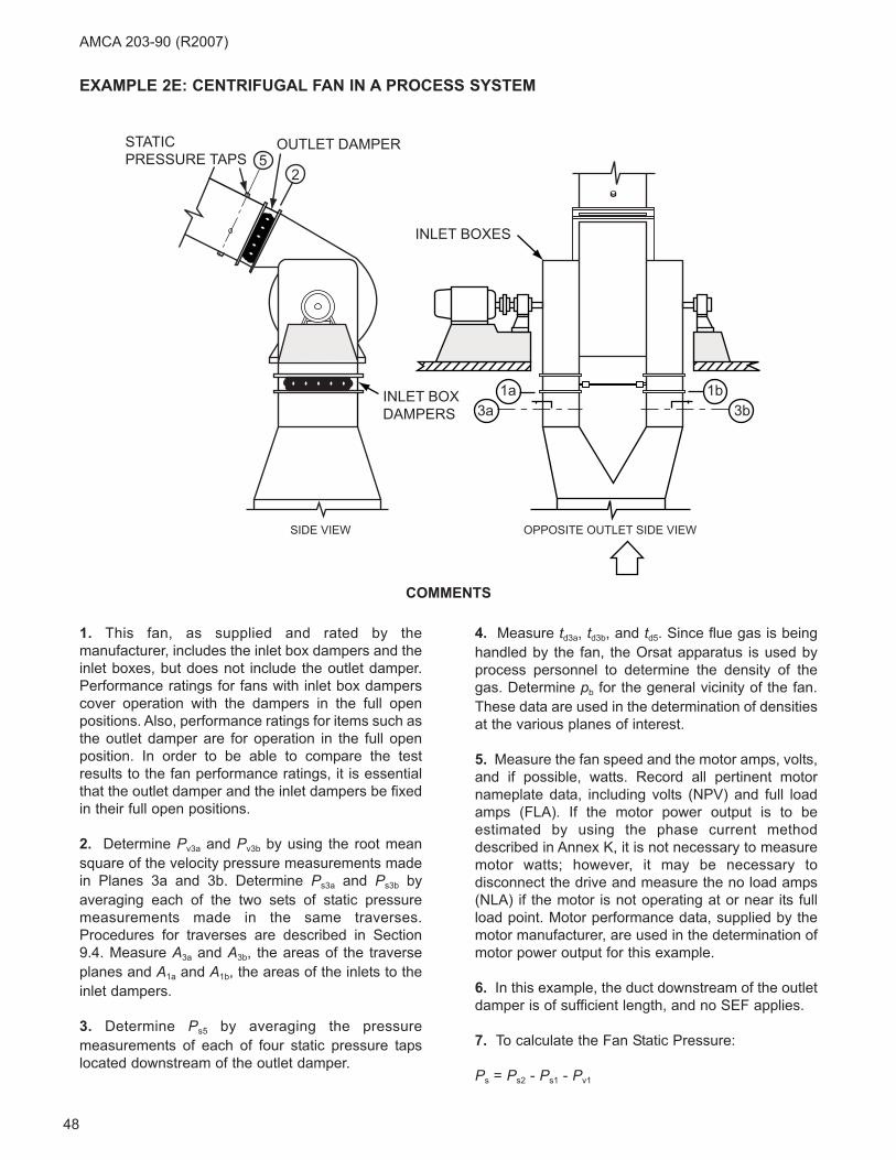
48
AMCA 203-90 (R2007)
1. This fan, as supplied and rated by the
manufacturer, includes the inlet box dampers and the
inlet boxes, but does not include the outlet damper.
Performance ratings for fans with inlet box dampers
cover operation with the dampers in the full open
positions. Also, performance ratings for items such as
the outlet damper are for operation in the full open
position. In order to be able to compare the test
results to the fan performance ratings, it is essential
that the outlet damper and the inlet dampers be fixed
in their full open positions.
2. Determine Pv3a and Pv3b by using the root mean
square of the velocity pressure measurements made
in Planes 3a and 3b. Determine Ps3a and Ps3b by
averaging each of the two sets of static pressure
measurements made in the same traverses.
Procedures for traverses are described in Section
9.4. Measure A3a and A3b, the areas of the traverse
planes and A1a and A1b, the areas of the inlets to the
inlet dampers.
3. Determine Ps5 by averaging the pressure
measurements of each of four static pressure taps
located downstream of the outlet damper.
4. Measure td3a, td3b, and td5. Since flue gas is being
handled by the fan, the Orsat apparatus is used by
process personnel to determine the density of the
gas. Determine pb for the general vicinity of the fan.
These data are used in the determination of densities
at the various planes of interest.
5. Measure the fan speed and the motor amps, volts,
and if possible, watts. Record all pertinent motor
nameplate data, including volts (NPV) and full load
amps (FLA). If the motor power output is to be
estimated by using the phase current method
described in Annex K, it is not necessary to measure
motor watts; however, it may be necessary to
disconnect the drive and measure the no load amps
(NLA) if the motor is not operating at or near its full
load point. Motor performance data, supplied by the
motor manufacturer, are used in the determination of
motor power output for this example.
6. In this example, the duct downstream of the outlet
damper is of sufficient length, and no SEF applies.
7. To calculate the Fan Static Pressure:
Ps = Ps2 - Ps1 - Pv1
EXAMPLE 2E: CENTRIFUGAL FAN IN A PROCESS SYSTEM
COMMENTS
STATICPRESSURE TAPS
OUTLET DAMPER
INLET BOXES
INLET BOXDAMPERS
52
SIDE VIEW OPPOSITE OUTLET SIDE VIEW
3a 3b1a 1b
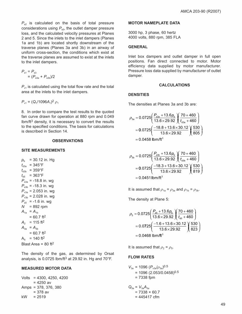
49
Ps2 is calculated on the basis of total pressure
considerations using Ps5, the outlet damper pressure
loss, and the calculated velocity pressures at Planes
2 and 5. Since the inlets to the inlet dampers (Planes
1a and 1b) are located shortly downstream of the
traverse planes (Planes 3a and 3b) in an airway of
uniform cross-section, the conditions which exist at
the traverse planes are assumed to exist at the inlets
to the inlet dampers.
Ps1 = Ps3
= (Ps3a + Ps3b)/2
Pv1 is calculated using the total flow rate and the total
area at the inlets to the inlet dampers.
Pv1 = (Q1/1096A1)2 ρ1
8. In order to compare the test results to the quoted
fan curve drawn for operation at 880 rpm and 0.049
lbm/ft3 density, it is necessary to convert the results
to the specified conditions. The basis for calculations
is described in Section 14.
OBSERVATIONS
SITE MEASUREMENTS
pb = 30.12 in. Hg
td3a = 345°F
td3b = 359°F
td5 = 363°F
Ps3a = -18.8 in. wg
Ps3b = -18.3 in. wg
Pv3a = 2.053 in. wg
Pv3b = 2.028 in. wg
Ps5 = -1.6 in. wg
N = 892 rpm
A1a = A1b
= 60.7 ft2
A2 = 115 ft2
A3a = A3b
= 60.7 ft2
A5 = 140 ft2
Blast Area = 80 ft2
The density of the gas, as determined by Orsat
analysis, is 0.0725 lbm/ft3 at 29.92 in. Hg and 70°F.
MEASURED MOTOR DATA
Volts = 4300, 4250, 4200
= 4250 av
Amps = 378, 376, 380
= 378 av
kW = 2519
MOTOR NAMEPLATE DATA
3000 hp, 3 phase, 60 hertz
4000 volts, 880 rpm, 385 FLA
GENERAL
Inlet box dampers and outlet damper in full open
positions. Fan direct connected to motor. Motor
efficiency data supplied by motor manufacturer.
Pressure loss data supplied by manufacturer of outlet
damper.
CALCULATIONS
DENSITIES
The densities at Planes 3a and 3b are:
It is assumed that ρ1a = ρ3a and ρ1b = ρ3b.
The density at Plane 5:
It is assumed that ρ2 = ρ5.
FLOW RATES
V3a = 1096 (Pv3a/ρ3a)0.5
= 1096 (2.053/0.0458)0.5
= 7338 fpm
Q3a = V3aA3a
= 7338 × 60.7
= 445417 cfm
ρ5s5 b
d5
= +×
⎛⎝⎜
⎞⎠⎟
++
⎛
⎝⎜
⎞
⎠⎟
=
0 072513 6
13 6 29 92
70 460
460
0 0
..
. .
.
P pt
77251 6 13 6 30 12
13 6 29 92
530
823
0 0468
− + ××
⎛⎝⎜
⎞⎠⎟⎛⎝⎜
⎞⎠⎟
=
. . .
. .
. lbm/fft3
ρ3bs3b b
d3b
= +×
⎛⎝⎜
⎞⎠⎟
++
⎛
⎝⎜
⎞
⎠⎟
=
0 072513 6
13 6 29 92
70 460
460.
.
. .
P pt
00 072518 3 13 6 30 12
13 6 29 92
530
819
0 0451
.. . .
. .
.
− + ××
⎛⎝⎜
⎞⎠⎟⎛⎝⎜
⎞⎠⎟
= llbm/ft3
ρ3as3a b
d3a
= +×
⎛⎝⎜
⎞⎠⎟
++
⎛
⎝⎜
⎞
⎠⎟
=
0 072513 6
13 6 29 92
70 460
460.
.
. .
P pt
00 072518 8 13 6 30 12
13 6 29 92
530
805
0 0458
.. . .
. .
.
− + ××
⎛⎝⎜
⎞⎠⎟⎛⎝⎜
⎞⎠⎟
= llbm/ft3
AMCA 203-90 (R2007)
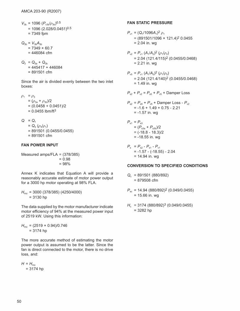
50
V3b = 1096 (Pv3b/ρ3b)0.5
= 1096 (2.028/0.0451)0.5
= 7349 fpm
Q3b = V3bA3b
= 7349 × 60.7
= 446084 cfm
Q3 = Q3a + Q3b
= 445417 + 446084
= 891501 cfm
Since the air is divided evenly between the two inlet
boxes:
ρ1 = ρ3
= (ρ3a + ρ3b)/2
= (0.0458 + 0.0451)/2
= 0.0455 lbm/ft3
Q = Q1
= Q3 (ρ3/ρ1)
= 891501 (0.0455/0.0455)
= 891501 cfm
FAN POWER INPUT
Measured amps/FLA = (378/385)
= 0.98
= 98%
Annex K indicates that Equation A will provide a
reasonably accurate estimate of motor power output
for a 3000 hp motor operating at 98% FLA.
Hmo = 3000 (378/385) (4250/4000)
= 3130 hp
The data supplied by the motor manufacturer indicate
motor efficiency of 94% at the measured power input
of 2519 kW. Using this information:
Hmo = (2519 × 0.94)/0.746
= 3174 hp
The more accurate method of estimating the motor
power output is assumed to be the latter. Since the
fan is direct connected to the motor, there is no drive
loss, and:
H = Hmo
= 3174 hp
FAN STATIC PRESSURE
Pv1 = (Q1/1096A1)2 ρ1
= (891501/1096 × 121.4)2 0.0455
= 2.04 in. wg
Pv2 = Pv1 (A1/A2)2 (ρ1/ρ2)
= 2.04 (121.4/115)2 (0.0455/0.0468)
= 2.21 in. wg
Pv5 = Pv1 (A1/A5)2 (ρ1/ρ5)
= 2.04 (121.4/140)2 (0.0455/0.0468)
= 1.49 in. wg
Ps2 + Pv2 = Ps5 + Pv5 + Damper Loss
Ps2 = Ps5 + Pv5 + Damper Loss - Pv2
= -1.6 + 1.49 + 0.75 - 2.21
= -1.57 in. wg
Ps1 = Ps3
= (Ps3a + Ps3b)/2
= (-18.8 - 18.3)/2
= -18.55 in. wg
Ps = Ps2 - Ps1 - Pv1
= -1.57 - (-18.55) - 2.04
= 14.94 in. wg
CONVERSION TO SPECIFIED CONDITIONS
Qc = 891501 (880/892)
= 879508 cfm
Psc = 14.94 (880/892)2 (0.049/0.0455)
= 15.66 in. wg
Hc = 3174 (880/892)3 (0.049/0.0455)
= 3282 hp
AMCA 203-90 (R2007)
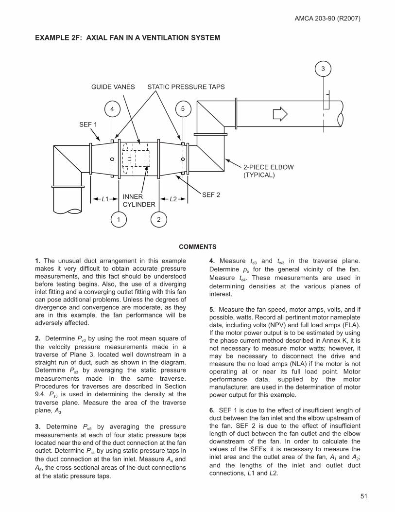
51
AMCA 203-90 (R2007)
1. The unusual duct arrangement in this example
makes it very difficult to obtain accurate pressure
measurements, and this fact should be understood
before testing begins. Also, the use of a diverging
inlet fitting and a converging outlet fitting with this fan
can pose additional problems. Unless the degrees of
divergence and convergence are moderate, as they
are in this example, the fan performance will be
adversely affected.
2. Determine Pv3 by using the root mean square of
the velocity pressure measurements made in a
traverse of Plane 3, located well downstream in a
straight run of duct, such as shown in the diagram.
Determine Ps3 by averaging the static pressure
measurements made in the same traverse.
Procedures for traverses are described in Section
9.4. Ps3 is used in determining the density at the
traverse plane. Measure the area of the traverse
plane, A3.
3. Determine Ps5 by averaging the pressure
measurements at each of four static pressure taps
located near the end of the duct connection at the fan
outlet. Determine Ps4 by using static pressure taps in
the duct connection at the fan inlet. Measure A4 and
A5, the cross-sectional areas of the duct connections
at the static pressure taps.
4. Measure td3 and tw3 in the traverse plane.
Determine pb for the general vicinity of the fan.
Measure td4. These measurements are used in
determining densities at the various planes of
interest.
5. Measure the fan speed, motor amps, volts, and if
possible, watts. Record all pertinent motor nameplate
data, including volts (NPV) and full load amps (FLA).
If the motor power output is to be estimated by using
the phase current method described in Annex K, it is
not necessary to measure motor watts; however, it
may be necessary to disconnect the drive and
measure the no load amps (NLA) if the motor is not
operating at or near its full load point. Motor
performance data, supplied by the motor
manufacturer, are used in the determination of motor
power output for this example.
6. SEF 1 is due to the effect of insufficient length of
duct between the fan inlet and the elbow upstream of
the fan. SEF 2 is due to the effect of insufficient
length of duct between the fan outlet and the elbow
downstream of the fan. In order to calculate the
values of the SEFs, it is necessary to measure the
inlet area and the outlet area of the fan, A1 and A2;
and the lengths of the inlet and outlet duct
connections, L1 and L2.
EXAMPLE 2F: AXIAL FAN IN A VENTILATION SYSTEM
COMMENTS
3
4 5
1 2
INNERCYLINDER
GUIDE VANES STATIC PRESSURE TAPS
SEF 1
SEF 2
2-PIECE ELBOW(TYPICAL)
L1 L2

52
7. To calculate the Fan Static Pressure:
Ps = Ps2 - Ps1 - Pv1 + SEF 1 + SEF 2
Where:
Pv1 = Pv3 (A3/A1)2 (ρ3/ρ1)
Ps2 and Ps1 are calculated using measured static
pressure values and constant total pressure
considerations.
Ps1 + Pv1 = Ps4 + Pv4
Ps2 + Pv2 = Ps5 + Pv5
Where each velocity pressure is calculated in a
manner similar to the calculation of Pv1, shown
above.
8. In order to compare the test results to the quoted
fan curve drawn for operation at 1750 rpm and 0.075
lbm/ft3 density, it is necessary to convert the results
to the specified conditions. The basis for the
calculations is described in Section 14.
OBSERVATIONS
SITE MEASUREMENTS
pb = 29.76 in. Hg
td3 = 82.8°F
tw3 = 57.2°F
td4 = 80°F
Ps3 = 0.5 in. wg
Pv3 = 0.783 in. wg
Ps4 = -1.1 in. wg
Ps5 = 0.82 in. wg
A1 = A2
= 7.1 ft2
A3 = A5
= 4.91 ft2
A4 = 6.2 ft2
L1 = 3.0 ft
L2 = 3.5 ft
MEASURED MOTOR DATA
Volts = 460, 461, 459
= 460 av
Amps = 25.0, 25.0, 24.8
= 24.9 av
kW = 18.0
MOTOR NAMEPLATE DATA
20 hp, 3 phase, 60 hertz
460 volts, 1760 rpm, 24.6 FLA
GENERAL
Fan direct connected to motor. Motor efficiency data
supplied by motor manufacturer. Fan speed
measurement was not obtained due to the closed
duct arrangements on both sides of the fan. The
measured amps indicate that the motor is operating
very close to the full load condition, so the rpm was
assumed to be the motor nameplate value of 1760.
CALCULATIONS
DENSITIES
For Plane 3 conditions of:
td3 = 82.8°F
tw3 = 57.2°F
p3 = pb + (Ps3/13.6)
= 29.76 + (0.5/13.6)
= 29.80 in. Hg
Use Figure N.1 in Annex N to obtain ρ3 = 0.0728
lbm/ft3.
It is assumed ρ2 = ρ5 = ρ3.
The density at Planes 1 and 4:
FLOW RATES
V3 = 1096 (Pv3/ρ3)0.5
= 1096 (0.783/0.0728)0.5
= 3594 fpm
Q3 = V3A3
= 3594 × 4.91
= 17647 cfm
Q = Q1
= Q3 (ρ3/ρ1)
= 17647 (0.0728/0.0729)
= 17623 cfm
ρ ρ
ρ
1 4
3
13 6
13 6
460
460
0 0728
=
= +⎛
⎝⎜
⎞
⎠⎟
++
⎛
⎝⎜
⎞
⎠⎟
= −
P pp
tt
s4 b
3
d3
d4
.
.
.11 1 13 6 29 76
13 6 29 80
542 8
540
0 0729
. . .
. .
.
.
+ ××
⎛⎝⎜
⎞⎠⎟⎛⎝⎜
⎞⎠⎟
= lbm/ft33
AMCA 203-90 (R2007)

53
FAN POWER INPUT
The data supplied by the motor manufacturer indicate
motor efficiency of 87.5% at the measured power
input of 18.0 kW. Using this information:
Hmo = (18.0 × 0.875)/0.746
= 21.1 hp
Since the fan is direct connected to the motor, there
is no drive loss, and:
H = Hmo
= 21.1 hp
SYSTEM EFFECT FACTORS
To determine the value of SEF 1, calculate the
velocity at the fan inlet:
V1 = (Q1/A1)
= (17623/7.1)
= 2482 fpm
Diameter of the fan inlet:
D1 = (4A1/π)0.5
= (4 × 7.1/π)0.5
= 3.01 ft
The length of the duct between the elbow and the fan
inlet in terms of the fan inlet diameter:
= (L1/D1)
= (3.0/3.01)
= 1.00
AMCA Publication 201-90, Figure 9.2 indicates that
for a two piece elbow with a length of duct between
the elbow and the fan inlet equal to 1.00 diameter
System Effect Curve S-T applies. For a velocity of
2482 fpm and curve S-T, Figure 7.1 shows SEF 1 =
0.25 in. wg at 0.075 lbm/ft3. At 0.0729 lbm/ft3:
SEF 1 = 0.25 (0.0729/0.075)
= 0.24 in. wg
For SEF 2, AMCA Publication 201-90, Figures 7.1,
8.1, and 8.4 indicate the following calculations:
Q2 = Q3 (ρ3/ρ2)
= 17647 (0.0728/0.0728)
= 17647 cfm
V2 = Q2/A2
= 17647/7.1
= 2485 fpm
Diameter of the fan outlet:
D2 = (4A2/π)0.5
= (4 × 7.1/π)0.5
= 3.01 ft
Figure 8.1 shows that for velocities of 2500 fpm or
less, the 100% effective duct length is 2.5 diameters:
= 2.5 × 3.01
= 7.53 ft
The length of the outlet duct in % effective duct
length:
= (L2/7.53) 100
= (3.5/7.53) 100
= 46%
From Figure 8.4, for a vaneaxial fan with a 46%
effective duct length between its discharge and a two
piece elbow, System Effect Curve W applies. From
Figure 7.1 for 2485 fpm velocity and curve W, SEF 2
is less than 0.1 in. and is considered negligible.
SEF 2 = 0.00
FAN STATIC PRESSURE
Pv5 = Pv3 (A3/A5)2 (ρ3/ρ5)
= 0.783 (4.91/4.91)2 (0.0728/0.0728)
= 0.783 in. wg
Pv2 = Pv3 (A3/A2)2 (ρ3/ρ2)
= 0.783 (4.91/7.1)2 (0.0728/0.0728)
= 0.37 in. wg
Ps2 + Pv2 = Ps5 + Pv5
Ps2 = Ps5 + Pv5 - Pv2
= 0.82 + 0.783 - 0.37
= 1.23 in. wg
Pv4 = Pv3 (A3/A4)2 (ρ3/ρ4)
= 0.783 (4.91/6.2)2 (0.0728/0.0729)
= 0.49 in. wg
Pv1 = Pv3 (A3/A1)2 (ρ3/ρ1)
= 0.783 (4.91/7.1)2 (0.0728/0.0729)
= 0.37 in. wg
Ps1 + Pv1 = Ps4 + Pv4
Ps1 = Ps4 + Pv4 - Pv1
= -1.1 + 0.49 - 0.37
= -0.98 in. wg
AMCA 203-90 (R2007)
54
Ps = Ps2 - Ps1 - Pv1 + SEF 1 + SEF 2
= 1.23 - (-0.98) - 0.37 + 0.24 + 0
= 2.08 in. wg
CONVERSION TO SPECIFIED CONDITIONS
Qc = 17623 (1750/1760)
= 17523 cfm
Psc = 2.08 (1750/1760)2 (0.075/0.0729)
= 2.12 in. wg
Hc = 21.1 (1750/1760)3 (0.075/0.0729)
= 21.3 hp
AMCA 203-90 (R2007)
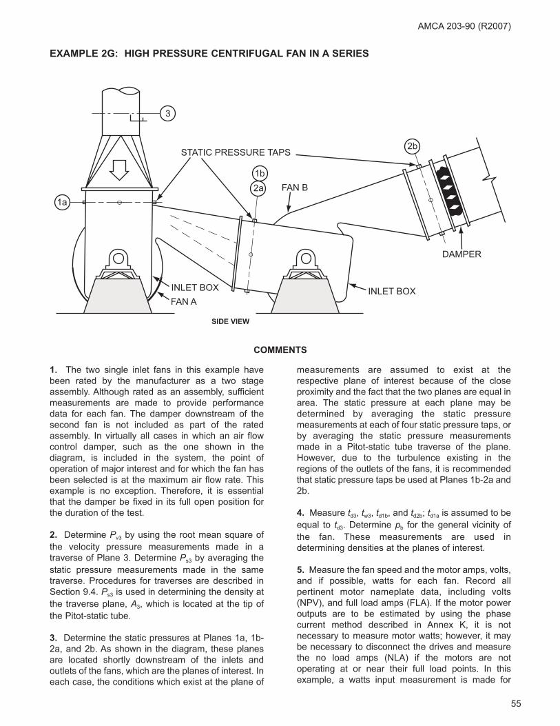
55
AMCA 203-90 (R2007)
1. The two single inlet fans in this example have
been rated by the manufacturer as a two stage
assembly. Although rated as an assembly, sufficient
measurements are made to provide performance
data for each fan. The damper downstream of the
second fan is not included as part of the rated
assembly. In virtually all cases in which an air flow
control damper, such as the one shown in the
diagram, is included in the system, the point of
operation of major interest and for which the fan has
been selected is at the maximum air flow rate. This
example is no exception. Therefore, it is essential
that the damper be fixed in its full open position for
the duration of the test.
2. Determine Pv3 by using the root mean square of
the velocity pressure measurements made in a
traverse of Plane 3. Determine Ps3 by averaging the
static pressure measurements made in the same
traverse. Procedures for traverses are described in
Section 9.4. Ps3 is used in determining the density at
the traverse plane, A3, which is located at the tip of
the Pitot-static tube.
3. Determine the static pressures at Planes 1a, 1b-
2a, and 2b. As shown in the diagram, these planes
are located shortly downstream of the inlets and
outlets of the fans, which are the planes of interest. In
each case, the conditions which exist at the plane of
measurements are assumed to exist at the
respective plane of interest because of the close
proximity and the fact that the two planes are equal in
area. The static pressure at each plane may be
determined by averaging the static pressure
measurements at each of four static pressure taps, or
by averaging the static pressure measurements
made in a Pitot-static tube traverse of the plane.
However, due to the turbulence existing in the
regions of the outlets of the fans, it is recommended
that static pressure taps be used at Planes 1b-2a and
2b.
4. Measure td3, tw3, td1b, and td2b; td1a is assumed to be
equal to td3. Determine pb for the general vicinity of
the fan. These measurements are used in
determining densities at the planes of interest.
5. Measure the fan speed and the motor amps, volts,
and if possible, watts for each fan. Record all
pertinent motor nameplate data, including volts
(NPV), and full load amps (FLA). If the motor power
outputs are to be estimated by using the phase
current method described in Annex K, it is not
necessary to measure motor watts; however, it may
be necessary to disconnect the drives and measure
the no load amps (NLA) if the motors are not
operating at or near their full load points. In this
example, a watts input measurement is made for
EXAMPLE 2G: HIGH PRESSURE CENTRIFUGAL FAN IN A SERIES
COMMENTS
3
STATIC PRESSURE TAPS
INLET BOXFAN A
INLET BOX
DAMPER
FAN B1a
1b2a
2b
SIDE VIEW

56
each motor and motor performance data, supplied by
the motor manufacturer, are used in determining
motor power outputs.
6. The SEF which would normally be attributed to
insufficient length of duct at the outlet of the first
stage fan does not apply in this case because the
fans have been rated as an assembly.
7. To calculate the static pressure for the two stage
assembly:
Ps = Ps2b - Ps1a - Pv1a
Where:
Pv1a = Pv3 (A3/A1a)2 (ρ3/ρ1a)
8. In order to compare the test results to the
performance quoted for the two stage assembly for
operation at 1780 rpm and 0.045 lbm/ft3 density, it is
necessary to convert the results to the specified
conditions. The basis for the calculations is described
in Section 14.
OBSERVATIONS
SITE MEASUREMENTS
pb = 28.64 in. Hg
td3 = 35°F
tw3 = 33°F
td1b = td2a
= 95°F
td2b = 147°F
Pv3 = 0.745 in. wg
Ps3 = -150 in. wg
Ps1b = Ps2a
= -79.5 in. wg
Ps2b = 0.5 in. wg
Na = 1790 rpm, first stage fan speed
Nb = 1790 rpm, second stage fan speed
A1a = A2a = A1b = A2b
= 5.6 ft2
A3 = 4.92 ft2
MEASURED MOTOR DATA
First Stage
Volts = 4000, 4040, 4080
= 4040 av
Amps = 44.5, 45, 45.5
= 45 av
kW = 278
Second Stage
Volts = 4080, 4040, 4020
= 4047 av
Amps = 44, 44.5, 45
= 44.5 av
kW = 272
MOTOR NAMEPLATE DATA
Data identical for each stage:
350 hp, 3 phase, 60 hertz
4000 volts, 1790 rpm, 44.5 FLA
GENERAL
Fans direct connected to motors. Motor efficiency
data supplied by motor manufacturer.
CALCULATIONS
DENSITIES
For Plane 3 conditions of:
td3 = 35°F
tw3 = 33°F
p3 = pb + (Ps3/13.6)
= 28.64 + (-150/13.6)
= 17.61 in. Hg
Use the modified Apjohn equation for partial vapor
pressure and the density equation based on perfect
gas relationships, both of which are described in
Annex M, and the data in Figure N.2 in Annex N to
calculate the density at Plane 3.
pe = 0.1879 in. Hg
Any conversion of velocity pressure to static pressure
which may occur between Planes 3 and 1a can be
ignored with no significant effect on the accuracy of
the test results. Therefore:
p p p t tp e
d3 w3
in. Hg
= − −
= − −
=
3
2700
0 187917 61 35 33
2700
0 1749
( )
.. ( )
.
ρ33
31 3257 0 378
460
1 3257 17 61 0 378 0 1749
35
=−
+
=− ×( )+
. ( . )
. . . .
p pt
p
d3
4460
0 0470 3= . lbm/ft
AMCA 203-90 (R2007)

57
AMCA 203-90 (R2007)
Ps1a = Ps3
= -150 in. wg
Assuming no change in temperature between Planes
3a and 1a:
ρ1a = ρ3
= 0.0470 lbm/ft3
To provide information regarding the flow rates
between stages and leaving the second stage,
additional density values are calculated as follows:
FLOW RATES
V3 = 1096 (Pv3/ρ3)0.5
= 1096 (0.745/0.0470)0.5
= 4364 fpm
Q3 = V3A3
= 4364 × 4.92
= 21471 cfm
Q = Q1a
= Q3 (ρ3/ρ1a)
= 21471 (0.0470/0.0470)
= 21471 cfm
Q1b = Q2a
= Q3 (ρ3/ρ2a)
= 21471 (0.0470/0.0543)
= 18584 cfm
Q2b = Q3 (ρ3/ρ2b)
= 21471 (0.0470/0.0624)
= 16172 cfm
FAN POWER INPUT
At the measured power input values of 278 kW and
272 kW, the data supplied by the motor manufacturer
indicate efficiency of 95% for each motor.
Hmoa = (278 × 0.95)/0.746
= 354 hp
Hmob = (272 × 0.95)/0.746
= 346 hp
Since each fan is direct connected to its motor, there
are no drive losses and:
Ha = Hmoa
= 354 hp
Hb = Hmob
= 346 hp
FAN STATIC PRESSURE
Pv1a = Pv3 (A3/A1a)2 (ρ3/ρ1a)
= 0.745 (4.92/5.6)2 (0.0470/0.0470)
= 0.575 in. wg
The static pressure for the two stage assembly:
Ps = Ps2b - Ps1a - Pv1a
= 0.5 - (-150) - 0.575
= 149.9 in. wg
CONVERSION TO SPECIFIED CONDITIONS
Qc = 21471 (1780/1790)
= 21351 cfm
Psc = 149.9 (1780/1790)2 (0.045/0.0470)
= 141.9 in. wg
Hac = 354 (1780/1790)3 (0.045/0.0470)
= 333 hp
Hbc = 346 (1780/1790)3 (0.045/0.0470)
= 326 hp
ρ ρ
ρ
1b 2a
s1b b d3
d4
=
= +⎛
⎝⎜
⎞
⎠⎟
++
⎛
⎝⎜
⎞
⎠⎟
=
3
3
13 6
13 6
460
460
0 04
P pp
tt
.
.
. 77079 5 13 6 28 64
13 6 17 61
495
555
0 0543
− + ××
⎛⎝⎜
⎞⎠⎟⎛⎝⎜
⎞⎠⎟
=
. . .
. .
. lbm/fft
2bs2b b d3
d2b
3
3
3
13 6
13 6
460
460
0 0
ρ ρ= +⎛
⎝⎜
⎞
⎠⎟
++
⎛
⎝⎜
⎞
⎠⎟
=
P pp
tt
.
.
. 44700 5 13 6 28 64
13 6 17 61
495
607
0 0624
. . .
. .
.
+ ××
⎛⎝⎜
⎞⎠⎟⎛⎝⎜
⎞⎠⎟
= lbm/ftt3
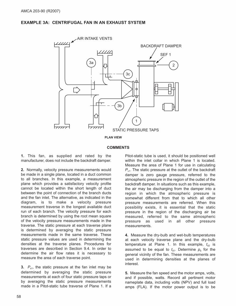
58
AMCA 203-90 (R2007)
1. This fan, as supplied and rated by the
manufacturer, does not include the backdraft damper.
2. Normally, velocity pressure measurements would
be made in a single plane, located in a duct common
to all branches. In this example, a measurement
plane which provides a satisfactory velocity profile
cannot be located within the short length of duct
between the point of connection of the branch ducts
and the fan inlet. The alternative, as indicated in the
diagram, is to make a velocity pressure
measurement traverse in the longest available duct
run of each branch. The velocity pressure for each
branch is determined by using the root mean square
of the velocity pressure measurements made in the
traverse. The static pressure at each traverse plane
is determined by averaging the static pressure
measurements made in the same traverse. These
static pressure values are used in determining the
densities at the traverse planes. Procedures for
traverses are described in Section 9.4. In order to
determine the air flow rates it is necessary to
measure the area of each traverse point.
3. Ps1, the static pressure at the fan inlet may be
determined by averaging the static pressure
measurements at each of four static pressure taps or
by averaging the static pressure measurements
made in a Pitot-static tube traverse of Plane 1. If a
Pitot-static tube is used, it should be positioned well
within the inlet collar in which Plane 1 is located.
Measure the area of Plane 1 for use in calculating
Pv1. The static pressure at the outlet of the backdraft
damper is zero gauge pressure, referred to the
atmospheric pressure in the region of the outlet of the
backdraft damper. In situations such as this example,
the air may be discharging from the damper into a
region in which the atmospheric pressure is
somewhat different from that to which all other
pressure measurements are referred. When this
possibility exists, it is essential that the static
pressure in the region of the discharging air be
measured, referred to the same atmospheric
pressure as used in all other pressure
measurements.
4. Measure the dry-bulb and wet-bulb temperatures
at each velocity traverse plane and the dry-bulb
temperature at Plane 1. In this example, td2 is
assumed to be equal to td1. Determine pb for the
general vicinity of the fan. These measurements are
used in determining densities at the planes of
interest.
5. Measure the fan speed and the motor amps, volts,
and if possible, watts. Record all pertinent motor
nameplate data, including volts (NPV) and full load
amps (FLA). If the motor power output is to be
EXAMPLE 3A: CENTRIFUGAL FAN IN AN EXHAUST SYSTEM
COMMENTS
3a
3c
3b
1
2
SEF 1
BACKDRAFT DAMPER
AIR INTAKE VENTS
STATIC PRESSURE TAPS
PLAN VIEW

59
estimated by using the phase current method
described in Annex K, it is not necessary to measure
motor watts; however, it may be necessary to
disconnect the drive and measure the no load amps
(NLA) if the motor is not operating at or near its full
load point. Refer to Annex K.
6. SEF 1 is due to the effect of there being no duct
at the fan outlet. In order to calculate the value of
SEF 1, it is necessary to measure the outlet area of
the fan, A2, and the blast area of the fan.
7. Determine the backdraft damper pressure loss by
using the performance ratings supplied by the
manufacturer and the pressure loss multiplier data in
Figure 8.7 of AMCA Publication 201-90. The use of
the multiplier is indicated because the damper is
mounted directly to the fan outlet.
8. To calculate the Fan Static Pressure:
Ps = Ps2 - Ps1 - Pv1 + SEF 1
Where:
Pv1 = (Q1/1096 A1)2 ρ1
Q1 = Q3a (ρ3a/ρ1) + Q3b (ρ3b/ρ1) + Q3c (ρ3c/ρ1)
Ps2 is the sum of the static pressure in the region of
the damper outlet, which was measured as zero, and
the backdraft damper pressure loss.
9. In order to compare the test results to the quoted
fan curve drawn for operation at 810 rpm and 0.075
lbm/ft3 density, it is necessary to convert the results
to the specified conditions. The basis for the
calculations is described in Section 14.
OBSERVATIONS
SITE MEASUREMENTS
pb = 29.8 in. Hg
td1 = 72°F
tw1 = 62°F
td3a = 77°F
tw3a = 67°F
td3b = 65°F
tw3b = 56°F
td3c = 70°F
tw3c = 62°F
Ps1 = -1.00 in. wg
Ps3a = -0.80 in. wg
Ps3b = -0.45 in. wg
Ps3c = -0.040 in. wg
Pv3a = 0.765 in. wg
Pv3b = 0.88 in. wg
Pv3c = 0.86 in. wg
N = 800 rpm
A1 = 16.8 ft2
A2 = 13.8 ft2
A3a = 5.4 ft2
A3b = A3c
= 3.0 ft2
Blast Area = 11.0 ft2
MEASURED MOTOR
Volts = 460, 458, 462
= 460 av
Amps = 28, 27, 26
= 27 av
NLA = 14.7
MOTOR NAMEPLATE DATA
25 hp, 3 phase, 60 hertz
460 volts, 1760 rpm, 32 FLA
GENERAL
Fan connected to motor through belt drive. Pressure
loss data supplied by manufacturer of backdraft
damper.
CALCULATIONS
DENSITIES
Since the static pressure values at Planes 1, 3a, 3b,
and 3c are very small, no appreciable error will occur
by using the barometric pressure instead of the
absolute pressure at each plane in the determination
of the densities. The densities at these planes are
obtained by using Figure N.1 in Annex N.
ρ1 = 0.0739 lbm/ft3
ρ3a = 0.0731 lbm/ft3
ρ3b = 0.0750 lbm/ft3
ρ3c = 0.0741 lbm/ft3
FLOW RATES
V3a = 1096 (Pv3a/ρ3a)0.5
= 1096 (0.765/0.0731)0.5
= 3546 fpm
V3b = 1096 (Pv3b/ρ3b)0.5
= 1096 (0.88/0.0750)0.5
= 3754 fpm
AMCA 203-90 (R2007)
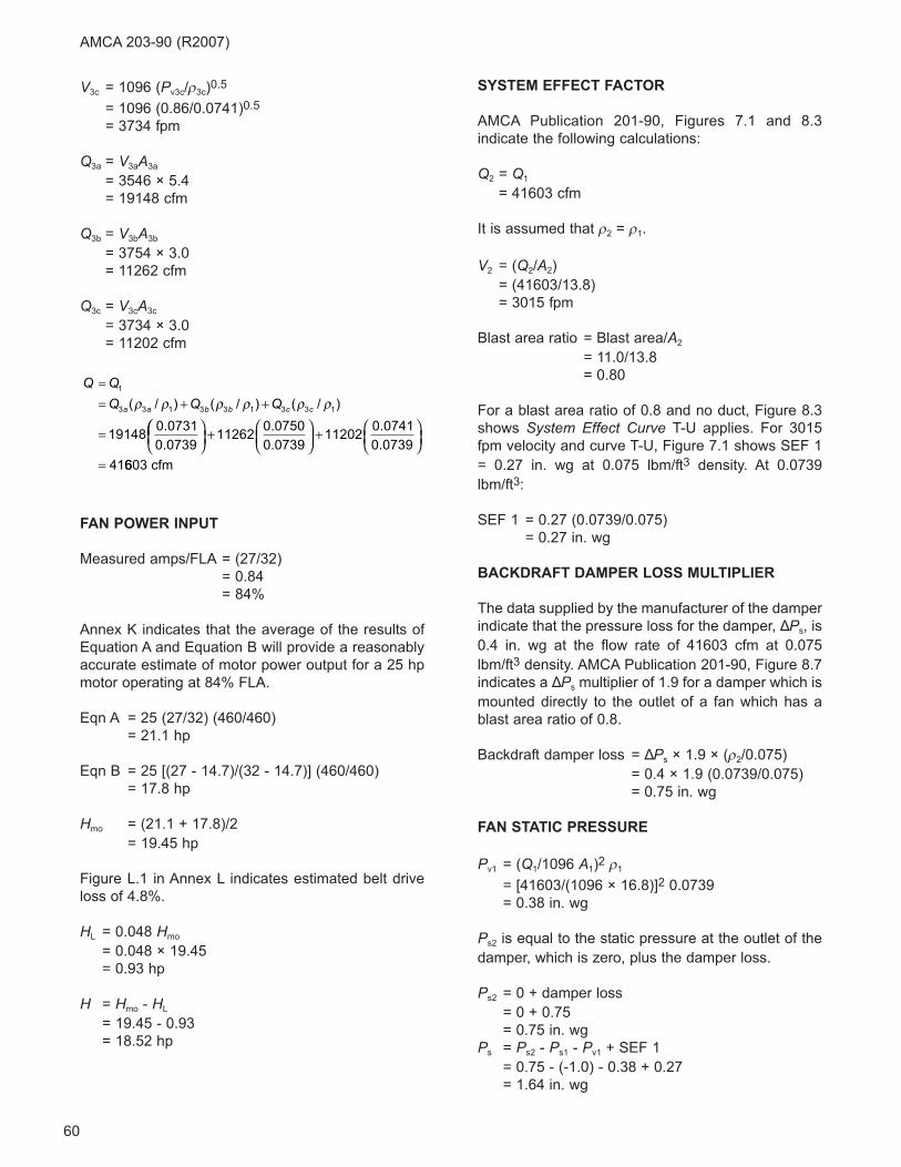
60
V3c = 1096 (Pv3c/ρ3c)0.5
= 1096 (0.86/0.0741)0.5
= 3734 fpm
Q3a = V3aA3a
= 3546 × 5.4
= 19148 cfm
Q3b = V3bA3b
= 3754 × 3.0
= 11262 cfm
Q3c = V3cA3c
= 3734 × 3.0
= 11202 cfm
FAN POWER INPUT
Measured amps/FLA = (27/32)
= 0.84
= 84%
Annex K indicates that the average of the results of
Equation A and Equation B will provide a reasonably
accurate estimate of motor power output for a 25 hp
motor operating at 84% FLA.
Eqn A = 25 (27/32) (460/460)
= 21.1 hp
Eqn B = 25 [(27 - 14.7)/(32 - 14.7)] (460/460)
= 17.8 hp
Hmo = (21.1 + 17.8)/2
= 19.45 hp
Figure L.1 in Annex L indicates estimated belt drive
loss of 4.8%.
HL = 0.048 Hmo
= 0.048 × 19.45
= 0.93 hp
H = Hmo - HL
= 19.45 - 0.93
= 18.52 hp
SYSTEM EFFECT FACTOR
AMCA Publication 201-90, Figures 7.1 and 8.3
indicate the following calculations:
Q2 = Q1
= 41603 cfm
It is assumed that ρ2 = ρ1.
V2 = (Q2/A2)
= (41603/13.8)
= 3015 fpm
Blast area ratio = Blast area/A2
= 11.0/13.8
= 0.80
For a blast area ratio of 0.8 and no duct, Figure 8.3
shows System Effect Curve T-U applies. For 3015
fpm velocity and curve T-U, Figure 7.1 shows SEF 1
= 0.27 in. wg at 0.075 lbm/ft3 density. At 0.0739
lbm/ft3:
SEF 1 = 0.27 (0.0739/0.075)
= 0.27 in. wg
BACKDRAFT DAMPER LOSS MULTIPLIER
The data supplied by the manufacturer of the damper
indicate that the pressure loss for the damper, ΔPs, is
0.4 in. wg at the flow rate of 41603 cfm at 0.075
lbm/ft3 density. AMCA Publication 201-90, Figure 8.7
indicates a ΔPs multiplier of 1.9 for a damper which is
mounted directly to the outlet of a fan which has a
blast area ratio of 0.8.
Backdraft damper loss = ΔPs × 1.9 × (ρ2/0.075)
= 0.4 × 1.9 (0.0739/0.075)
= 0.75 in. wg
FAN STATIC PRESSURE
Pv1 = (Q1/1096 A1)2 ρ1
= [41603/(1096 × 16.8)]2 0.0739
= 0.38 in. wg
Ps2 is equal to the static pressure at the outlet of the
damper, which is zero, plus the damper loss.
Ps2 = 0 + damper loss
= 0 + 0.75
= 0.75 in. wg
Ps = Ps2 - Ps1 - Pv1 + SEF 1
= 0.75 - (-1.0) - 0.38 + 0.27
= 1.64 in. wg
Q QQ Q Qa a b b c c
== + +
=
1
3 3 1 3 3 1 3 3 1
191480 0731
0 0739
( / ) ( / ) ( / )
.
.
ρ ρ ρ ρ ρ ρ
⎛⎛⎝⎜
⎞⎠⎟
+ ⎛⎝⎜
⎞⎠⎟
+ ⎛⎝⎜
⎞⎠⎟
=
112620 0750
0 073911202
0 0741
0 0739
41
.
.
.
.
6603 cfm
AMCA 203-90 (R2007)
61
CONVERSION TO SPECIFIED CONDITIONS
Qc = 41603 (810/800)
= 42123 cfm
Psc = 1.64 (810/800)2 (0.075/0.0739)
= 1.71 in. wg
Hc = 18.52 (810/800)3 (0.075/0.0739)
= 19.51 hp
AMCA 203-90 (R2007)
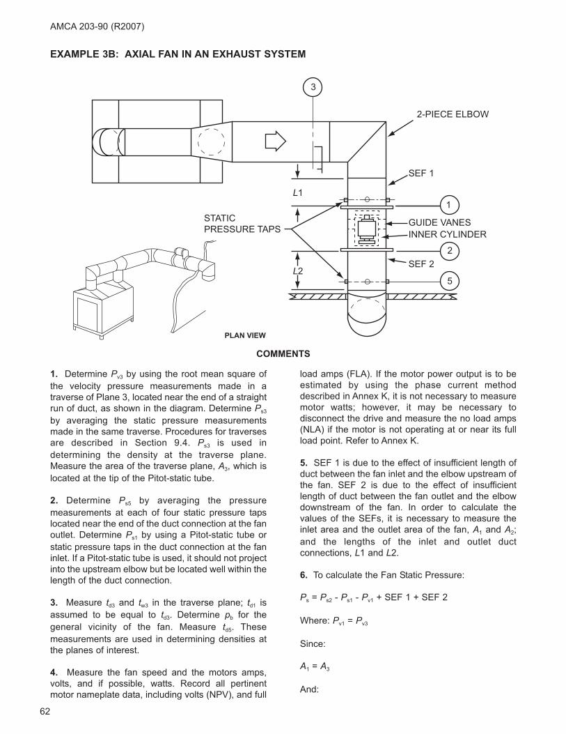
62
AMCA 203-90 (R2007)
1. Determine Pv3 by using the root mean square of
the velocity pressure measurements made in a
traverse of Plane 3, located near the end of a straight
run of duct, as shown in the diagram. Determine Ps3
by averaging the static pressure measurements
made in the same traverse. Procedures for traverses
are described in Section 9.4. Ps3 is used in
determining the density at the traverse plane.
Measure the area of the traverse plane, A3, which is
located at the tip of the Pitot-static tube.
2. Determine Ps5 by averaging the pressure
measurements at each of four static pressure taps
located near the end of the duct connection at the fan
outlet. Determine Ps1 by using a Pitot-static tube or
static pressure taps in the duct connection at the fan
inlet. If a Pitot-static tube is used, it should not project
into the upstream elbow but be located well within the
length of the duct connection.
3. Measure td3 and tw3 in the traverse plane; td1 is
assumed to be equal to td3. Determine pb for the
general vicinity of the fan. Measure td5. These
measurements are used in determining densities at
the planes of interest.
4. Measure the fan speed and the motors amps,
volts, and if possible, watts. Record all pertinent
motor nameplate data, including volts (NPV), and full
load amps (FLA). If the motor power output is to be
estimated by using the phase current method
described in Annex K, it is not necessary to measure
motor watts; however, it may be necessary to
disconnect the drive and measure the no load amps
(NLA) if the motor is not operating at or near its full
load point. Refer to Annex K.
5. SEF 1 is due to the effect of insufficient length of
duct between the fan inlet and the elbow upstream of
the fan. SEF 2 is due to the effect of insufficient
length of duct between the fan outlet and the elbow
downstream of the fan. In order to calculate the
values of the SEFs, it is necessary to measure the
inlet area and the outlet area of the fan, A1 and A2;
and the lengths of the inlet and outlet duct
connections, L1 and L2.
6. To calculate the Fan Static Pressure:
Ps = Ps2 - Ps1 - Pv1 + SEF 1 + SEF 2
Where: Pv1 = Pv3
Since:
A1 = A3
And:
EXAMPLE 3B: AXIAL FAN IN AN EXHAUST SYSTEM
COMMENTS
3
1
2
5
SEF 1
2-PIECE ELBOW
STATICPRESSURE TAPS
PLAN VIEW
SEF 2
GUIDE VANESINNER CYLINDER
L1
L2

63
ρ1 = ρ3
Due to the close proximity of Planes 2 and 5 and the
fact that there is no change in area between the two
planes, all conditions which exist at Plane 5 are
assumed to exist at Plane 2.
Therefore:
Ps2 = Ps5
7. In order to compare the test results to the quoted
fan curve drawn for operation at 1730 rpm and 0.075
lbm/ft3 density, it is necessary to convert the results
to the specified conditions. The basis for the
calculations is described in Section 14.
OBSERVATIONS
SITE MEASUREMENTS
pb = 29.20 in. Hg
td3 = 72°F
tw3 = 66°F
td5 = 73°F
Ps1 = -2.02 in. wg
Ps3 = -1.92 in. wg
Pv3 = 0.35 in. wg
Ps5 = 0.10 in. wg
N = 1710 rpm
A1 = A2 = A3 = A5
= 2.64 ft2
L1 = 1.5 ft, length of inlet duct
L2 = 2.25 ft, length of the outlet duct
MEASURED MOTOR DATA
Volts = 227, 229, 228
= 228 av
Amps = 12.2, 12.3, 12.4
= 12.3 av
NLA = 7
MOTOR NAMEPLATE DATA
5 hp, 3 phase, 60 hertz
230 volts, 1760 rpm, 14.0 FLA
GENERAL
Fan connected to motor through belt drive.
CALCULATIONS
DENSITIES
For Plane 3 conditions of:
td3 = 72°F
tw3 = 66°F
p3 = pb + (Ps3/13.6)
= 29.20 + (-1.92/13.6)
= 29.06 in. Hg
Use Figure N.1 in Annex N to obtain ρ3 = 0.0719
lbm/ft3.
Assume that td1 = td3.
Assume that td2 = td5 and Ps2 = Ps5.
FLOW RATES
V3 = 1096 (Pv3/ρ3)0.5
= 1096 (0.35/0.0719)0.5
= 2418 fpm
Q3 = V3A3
= 2418 × 2.64
= 6384 cfm
Q = Q1
= Q3 (ρ3/ρ1)
= 6384 (0.0719/0.0719)
= 6384 cfm
Q2 = Q5
= Q3 (ρ3/ρ5)
= 6384 (0.0719/0.0721)
= 6366 cfm
ρ ρ
ρ
2
s5 b
3
d3
d5
=
= +⎛
⎝⎜
⎞
⎠⎟
++
⎛
⎝⎜
⎞
⎠⎟
=
5
3
13 6
13 6
460
460
0 07190
P pp
tt
.
.
... . .
. .
.
10 13 6 29 20
13 6 29 06
532
533
0 0721
+ ××
⎛⎝⎜
⎞⎠⎟⎛⎝⎜
⎞⎠⎟
= lbm/ft3
ρ ρ1s1 b
3
d3
d1
= +⎛
⎝⎜
⎞
⎠⎟
++
⎛
⎝⎜
⎞
⎠⎟
= −
3
13 6
13 6
460
460
0 07192 0
P pp
tt
.
.
.. 22 13 6 29 20
13 6 29 06
532
532
0 0719
+ ××
⎛⎝⎜
⎞⎠⎟⎛⎝⎜
⎞⎠⎟
=
. .
. .
. lbm/ft3
AMCA 203-90 (R2007)
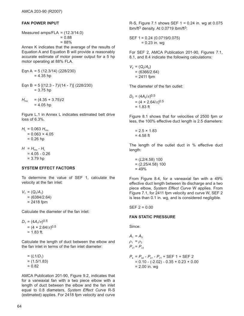
64
FAN POWER INPUT
Measured amps/FLA = (12.3/14.0)
= 0.88
= 88%
Annex K indicates that the average of the results of
Equation A and Equation B will provide a reasonably
accurate estimate of motor power output for a 5 hp
motor operating at 88% FLA.
Eqn A = 5 (12.3/14) (228/230)
= 4.35 hp
Eqn B = 5 [(12.3 - 7)/(14 - 7)] (228/230)
= 3.75 hp
Hmo = (4.35 + 3.75)/2
= 4.05 hp
Figure L.1 in Annex L indicates estimated belt drive
loss of 6.3%.
HL = 0.063 Hmo
= 0.063 × 4.05
= 0.26 hp
H = Hmo - HL
= 4.05 - 0.26
= 3.79 hp
SYSTEM EFFECT FACTORS
To determine the value of SEF 1, calculate the
velocity at the fan inlet:
V1 = (Q1/A1)
= (6384/2.64)
= 2418 fpm
Calculate the diameter of the fan inlet:
D1 = (4A1/π)0.5
= (4 × 2.64/π)0.5
= 1.83 ft.
Calculate the length of duct between the elbow and
the fan inlet in terms of the fan inlet diameter:
= (L1/D1)
= (1.5/1.83)
= 0.82
AMCA Publication 201-90, Figure 9.2, indicates that
for a vaneaxial fan with a two piece elbow with a
length of duct between the elbow and the fan inlet
equal to 0.8 diameters, System Effect Curve R-S
(estimated) applies. For 2418 fpm velocity and curve
R-S, Figure 7.1 shows SEF 1 = 0.24 in. wg at 0.075
lbm/ft3 density. At 0.0719 lbm/ft3:
SEF 1 = 0.24 (0.0719/0.075)
= 0.23 in. wg
For SEF 2, AMCA Publication 201-90, Figures 7.1,
8.1, and 8.4 indicate the following calculations:
V2 = (Q2/A2)
= (6366/2.64)
= 2411 fpm
The diameter of the fan outlet:
D2 = (4A2/π)0.5
= (4 × 2.64/π)0.5
= 1.83 ft
Figure 8.1 shows that for velocities of 2500 fpm or
less, the 100% effective duct length is 2.5 diameters:
= 2.5 × 1.83
= 4.58 ft
The length of the outlet duct in % effective duct
length:
= (L2/4.58) 100
= (2.25/4.58) 100
= 49%
From Figure 8.4, for a vaneaxial fan with a 49%
effective duct length between its discharge and a two
piece elbow, System Effect Curve W applies. From
Figure 7.1, for 2411 fpm velocity and curve W, SEF 2
is less than 0.1 in. wg, and is considered negligible.
SEF 2 = 0.00
FAN STATIC PRESSURE
Since:
A1 = A3
ρ1 = ρ3
Pv1 = Pv3
Ps = Ps2 - Ps1 - Pv1 + SEF 1 + SEF 2
= 0.10 - (-2.02) - 0.35 + 0.23 + 0.00
= 2.00 in. wg
AMCA 203-90 (R2007)
65
CONVERSION TO SPECIFIED CONDITIONS
Qc = 6384 (1730/1710)
= 6459 cfm
Psc = 2.00 (1730/1710)2 (0.075/0.0719)
= 2.14 in. wg
Hc = 3.79 (1730/1710)3 (0.075/0.0719)
= 4.09 hp
AMCA 203-90 (R2007)
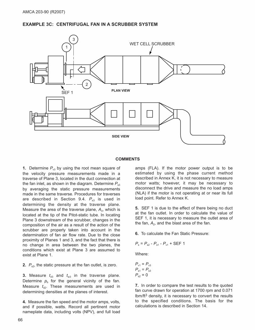
66
AMCA 203-90 (R2007)
1. Determine Pv3 by using the root mean square of
the velocity pressure measurements made in a
traverse of Plane 3, located in the duct connection at
the fan inlet, as shown in the diagram. Determine Ps3
by averaging the static pressure measurements
made in the same traverse. Procedures for traverses
are described in Section 9.4. Ps3 is used in
determining the density at the traverse plane.
Measure the area of the traverse plane, A3, which is
located at the tip of the Pitot-static tube. In locating
Plane 3 downstream of the scrubber, changes in the
composition of the air as a result of the action of the
scrubber are properly taken into account in the
determination of fan air flow rate. Due to the close
proximity of Planes 1 and 3, and the fact that there is
no change in area between the two planes, the
conditions which exist at Plane 3 are assumed to
exist at Plane 1.
2. Ps2, the static pressure at the fan outlet, is zero.
3. Measure td3 and tw3 in the traverse plane.
Determine pb for the general vicinity of the fan.
Measure td2. These measurements are used in
determining densities at the planes of interest.
4. Measure the fan speed and the motor amps, volts,
and if possible, watts. Record all pertinent motor
nameplate data, including volts (NPV), and full load
amps (FLA). If the motor power output is to be
estimated by using the phase current method
described in Annex K, it is not necessary to measure
motor watts; however, it may be necessary to
disconnect the drive and measure the no load amps
(NLA) if the motor is not operating at or near its full
load point. Refer to Annex K.
5. SEF 1 is due to the effect of there being no duct
at the fan outlet. In order to calculate the value of
SEF 1, it is necessary to measure the outlet area of
the fan, A2, and the blast area of the fan.
6. To calculate the Fan Static Pressure:
Ps = Ps2 - Ps1 - Pv1 + SEF 1
Where:
Pv1 = Pv3
Ps1 = Ps3
Ps2 = 0
7. In order to compare the test results to the quoted
fan curve drawn for operation at 1700 rpm and 0.071
lbm/ft3 density, it is necessary to convert the results
to the specified conditions. The basis for the
calculations is described in Section 14.
COMMENTS
WET CELL SCRUBBER
SEF 1 PLAN VIEW
SIDE VIEW
3
1
2
EXAMPLE 3C: CENTRIFUGAL FAN IN A SCRUBBER SYSTEM
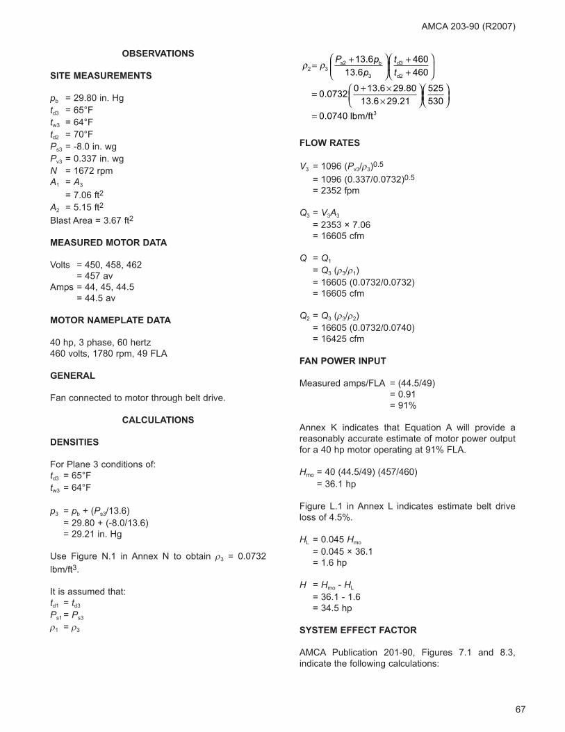
67
OBSERVATIONS
SITE MEASUREMENTS
pb = 29.80 in. Hg
td3 = 65°F
tw3 = 64°F
td2 = 70°F
Ps3 = -8.0 in. wg
Pv3 = 0.337 in. wg
N = 1672 rpm
A1 = A3
= 7.06 ft2
A2 = 5.15 ft2
Blast Area = 3.67 ft2
MEASURED MOTOR DATA
Volts = 450, 458, 462
= 457 av
Amps = 44, 45, 44.5
= 44.5 av
MOTOR NAMEPLATE DATA
40 hp, 3 phase, 60 hertz
460 volts, 1780 rpm, 49 FLA
GENERAL
Fan connected to motor through belt drive.
CALCULATIONS
DENSITIES
For Plane 3 conditions of:
td3 = 65°F
tw3 = 64°F
p3 = pb + (Ps3/13.6)
= 29.80 + (-8.0/13.6)
= 29.21 in. Hg
Use Figure N.1 in Annex N to obtain ρ3 = 0.0732
lbm/ft3.
It is assumed that:
td1 = td3
Ps1 = Ps3
ρ1 = ρ3
FLOW RATES
V3 = 1096 (Pv3/ρ3)0.5
= 1096 (0.337/0.0732)0.5
= 2352 fpm
Q3 = V3A3
= 2353 × 7.06
= 16605 cfm
Q = Q1
= Q3 (ρ3/ρ1)
= 16605 (0.0732/0.0732)
= 16605 cfm
Q2 = Q3 (ρ3/ρ2)
= 16605 (0.0732/0.0740)
= 16425 cfm
FAN POWER INPUT
Measured amps/FLA = (44.5/49)
= 0.91
= 91%
Annex K indicates that Equation A will provide a
reasonably accurate estimate of motor power output
for a 40 hp motor operating at 91% FLA.
Hmo = 40 (44.5/49) (457/460)
= 36.1 hp
Figure L.1 in Annex L indicates estimate belt drive
loss of 4.5%.
HL = 0.045 Hmo
= 0.045 × 36.1
= 1.6 hp
H = Hmo - HL
= 36.1 - 1.6
= 34.5 hp
SYSTEM EFFECT FACTOR
AMCA Publication 201-90, Figures 7.1 and 8.3,
indicate the following calculations:
ρ ρ2s2 b
3
d3
d2
= +⎛
⎝⎜
⎞
⎠⎟
++
⎛
⎝⎜
⎞
⎠⎟
= +
3
13 6
13 6
460
460
0 07320 13
P pp
tt
.
.
... .
. .
.
6 29 80
13 6 29 21
525
530
0 0740
××
⎛⎝⎜
⎞⎠⎟⎛⎝⎜
⎞⎠⎟
= lbm/ft3
AMCA 203-90 (R2007)

68
V2 = (Q2/A2)
= (16425/5.15)
= 3189 fpm
Blast area ratio = Blast area/A2
= 3.67/5.15
= 0.71
For a blast area ratio of 0.7 and no duct, Figure 8.3
shows System Effect Curve S applies. For 3189 fpm
velocity and curve S, Figure 7.1 shows SEF 1 = 0.5
in. wg at 0.075 lbm/ft3 density. At 0.0740 lbm/ft3:
SEF 1 = 0.5 (0.074/0.075)
= 0.49 in. wg
FAN STATIC PRESSURE
Pv1 = Pv3
= 0.337 in. wg
Ps = Ps2 - Ps1 - Pv1 + SEF 1
= 0 - (-8.0) - 0.337 + 0.49
= 8.15 in. wg
CONVERSION TO SPECIFIED CONDITIONS
Qc = 16605 (1700/1672)
= 16883 cfm
Psc = 8.15 (1700/1672)2 (0.071/0.0732)
= 8.17 in. wg
Hc = 34.5 (1700/1672)3 (0.071/0.0732)
= 35.2 hp
AMCA 203-90 (R2007)
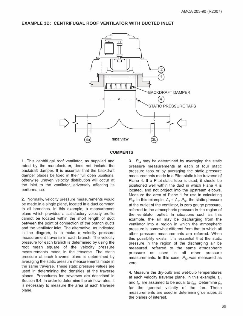
69
AMCA 203-90 (R2007)
1. This centrifugal roof ventilator, as supplied and
rated by the manufacturer, does not include the
backdraft damper. It is essential that the backdraft
damper blades be fixed in their full open positions,
otherwise uneven velocity distribution will occur at
the inlet to the ventilator, adversely affecting its
performance.
2. Normally, velocity pressure measurements would
be made in a single plane, located in a duct common
to all branches. In this example, a measurement
plane which provides a satisfactory velocity profile
cannot be located within the short length of duct
between the point of connection of the branch ducts
and the ventilator inlet. The alternative, as indicated
in the diagram, is to make a velocity pressure
measurement traverse in each branch. The velocity
pressure for each branch is determined by using the
root mean square of the velocity pressure
measurements made in the traverse. The static
pressure at each traverse plane is determined by
averaging the static pressure measurements made in
the same traverse. These static pressure values are
used in determining the densities at the traverse
planes. Procedures for traverses are described in
Section 9.4. In order to determine the air flow rates, it
is necessary to measure the area of each traverse
plane.
3. Ps4 may be determined by averaging the static
pressure measurements at each of four static
pressure taps or by averaging the static pressure
measurements made in a Pitot-static tube traverse of
Plane 4. If a Pitot-static tube is used, it should be
positioned well within the duct in which Plane 4 is
located, and not project into the upstream elbows.
Measure the area of Plane 1 for use in calculating
Pv1. In this example, A4 = A1. Ps2, the static pressure
at the outlet of the ventilator, is zero gauge pressure,
referred to the atmospheric pressure in the region of
the ventilator outlet. In situations such as this
example, the air may be discharging from the
ventilator into a region in which the atmospheric
pressure is somewhat different from that to which all
other pressure measurements are referred. When
this possibility exists, it is essential that the static
pressure in the region of the discharging air be
measured, referred to the same atmospheric
pressure as used in all other pressure
measurements. In this case, Ps2 was measured as
zero.
4. Measure the dry-bulb and wet-bulb temperatures
at each velocity traverse plane. In this example, td1
and td4 are assumed to be equal to td3a. Determine pb
for the general vicinity of the fan. These
measurements are used in determining densities at
the planes of interest.
COMMENTS
BACKDRAFT DAMPER
STATIC PRESSURE TAPS
3a 3b
2
1
4
SIDE VIEW
EXAMPLE 3D: CENTRIFUGAL ROOF VENTILATOR WITH DUCTED INLET

70
5. Measure the fan speed and the motor amps, volts,
and if possible, watts. Record all pertinent motor
nameplate data, including volts (NPV) and full load
amps (FLA). If the motor power output is to be
estimated by using the phase current method
described in Annex K, it is not necessary to measure
motor watts; however, it may be necessary to
disconnect the drive and measure the no load amps
(NLA) if the motor is not operating at or near its full
load point. Refer to Annex K.
6. Determine the backdraft damper pressure loss by
using the performance ratings supplied by the
manufacturer.
7. To calculate the Fan Static Pressure:
Ps = Ps2 - Ps1 - Pv1
Where:
Pv1 = (Q1/1096 A1)2 ρ1
Q1 = Q3a (ρ3a/ρ1) + Q3b (ρ3b/ρ1)
Ps1 = Ps4 - backdraft damper pressure loss
Ps2 = 0
8. In order to compare the test results to the quoted
fan curve drawn for operation at 620 rpm and 0.075
lbm/ft3 density, it is necessary to convert the results
to the specified conditions. The basis for the
calculations is described in Section 14.
OBSERVATIONS
SITE MEASUREMENTS
pb = 29.20 in. Hg
td3a = td3b
= 72°F
tw3a = tw3b
= 66°F
Ps2 = 0 in. wg
Ps4 = -0.88 in. wg
Ps3a = Ps3b
= -0.85 in. wg
Pv3a = 0.27 in. wg
Pv3b = 0.275 in. wg
N = 625 rpm
A1 = A4
= 7.9 ft2
A3a = 3.4 ft2
A3b = 3.3 ft2
MEASURED MOTOR DATA
Volts = 450, 455, 460
= 455 av
Amps = 5.7, 5.85, 5.9
= 5.82 av
MOTOR NAMEPLATE DATA
5 hp, 3 phase, 60 hertz
460 volts, 1780 rpm, 5.95 FLA
GENERAL
Fan connected to motor through belt drive. Pressure
loss data supplied by manufacturer of backdraft
damper.
CALCULATIONS
DENSITIES
For Planes 3a and 3b conditions of:
td3a = td3b
= 72°F
tw3a = tw3b
= 66°F
p3a = p3b
= pb + (Ps3a/13.6)
= 29.20 + (-0.85/13.6)
= 29.14 in. Hg
Use Figure N.1 in Annex N to obtain:
ρ3a = ρ3b
= 0.0721 lbm/ft3
It is assumed that:
td1 = td4 = td3a = td3b
Since the differences in the static pressures at
Planes 1, 3a, and 4 are very small, no appreciable
error will occur by assuming:
ρ1 = ρ4 = ρ3a = ρ3b
FLOW RATES
V3a = 1096 (Pv3a/ρ3a)0.5
= 1096 (0.27/0.0721)0.5
= 2121 fpm
AMCA 203-90 (R2007)
71
V3b = 1096 (Pv3b/ρ3b)0.5
= 1096 (0.275/0.0721)0.5
= 2140 fpm
Q3a = V3aA3a
= 2121 × 3.4
= 7211 cfm
Q3b = V3bA3b
= 2140 × 3.3
= 7062 cfm
Q = Q1
= Q3a (ρ3a/ρ1) + Q3b (ρ3b/ρ1)
= 7211 (0.0721/0.0721) + 7062 (0.0721/0.0721)
= 14273 cfm
FAN POWER INPUT
Measured amps/FLA = (5.82/5.95)
= 0.98
= 98%
Annex K indicates that Equation A will provide a
reasonably accurate estimate of motor power output
for a 5 hp motor operating at 98% FLA.
Hmo = 5 (5.82/5.95) (455/460)
= 4.84 hp
Figure L.1 in Annex L indicates estimated belt drive
loss of 5.8%.
HL = 0.058 Hmo
= 0.058 × 4.84
= 0.28 hp
H = Hmo - HL
= 4.84 - 0.28
= 4.56 hp
BACKDRAFT DAMPER LOSS
The data supplied by the manufacturer of the damper
indicate that the pressure loss for the damper, ΔPs, is
0.22 in. wg at the flow rate of 14273 cfm at 0.075
lbm/ft3 density.
Backdraft damper loss = ΔPs (ρ4/0.075)
= 0.22 (0.0721/0.075)
= 0.21 in. wg
FAN STATIC PRESSURE
Pv1 = (Q1/1096 A1)2 ρ1
= [14273/(1096 × 7.9)]2 0.0721
= 0.20 in. wg
Ps1 = Ps4 - damper loss
= -0.88 - 0.21
= -1.09 in. wg
Ps = Ps2 - Ps1 - Pv1
= 0 - (-1.09) - 0.20
= 0.89 in. wg
CONVERSION TO SPECIFIED CONDITIONS
Qc = 14273 (620/625)
= 14159 cfm
Psc = 0.89 (620/625)2 (0.075/0.0721)
= 0.91 in. wg
Hc = 4.56 (620/625)3 (0.075/0.0721)
= 4.63 hp
AMCA 203-90 (R2007)
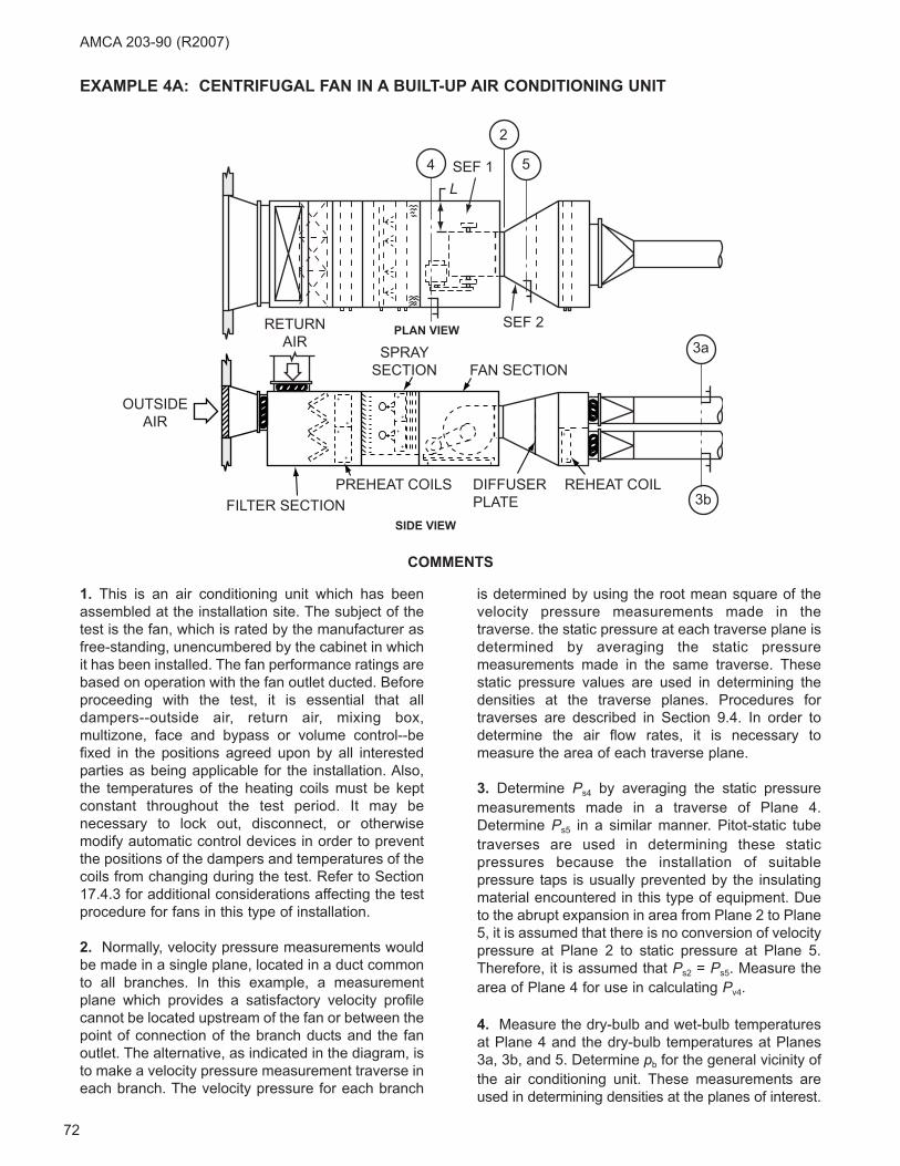
72
AMCA 203-90 (R2007)
1. This is an air conditioning unit which has been
assembled at the installation site. The subject of the
test is the fan, which is rated by the manufacturer as
free-standing, unencumbered by the cabinet in which
it has been installed. The fan performance ratings are
based on operation with the fan outlet ducted. Before
proceeding with the test, it is essential that all
dampers--outside air, return air, mixing box,
multizone, face and bypass or volume control--be
fixed in the positions agreed upon by all interested
parties as being applicable for the installation. Also,
the temperatures of the heating coils must be kept
constant throughout the test period. It may be
necessary to lock out, disconnect, or otherwise
modify automatic control devices in order to prevent
the positions of the dampers and temperatures of the
coils from changing during the test. Refer to Section
17.4.3 for additional considerations affecting the test
procedure for fans in this type of installation.
2. Normally, velocity pressure measurements would
be made in a single plane, located in a duct common
to all branches. In this example, a measurement
plane which provides a satisfactory velocity profile
cannot be located upstream of the fan or between the
point of connection of the branch ducts and the fan
outlet. The alternative, as indicated in the diagram, is
to make a velocity pressure measurement traverse in
each branch. The velocity pressure for each branch
is determined by using the root mean square of the
velocity pressure measurements made in the
traverse. the static pressure at each traverse plane is
determined by averaging the static pressure
measurements made in the same traverse. These
static pressure values are used in determining the
densities at the traverse planes. Procedures for
traverses are described in Section 9.4. In order to
determine the air flow rates, it is necessary to
measure the area of each traverse plane.
3. Determine Ps4 by averaging the static pressure
measurements made in a traverse of Plane 4.
Determine Ps5 in a similar manner. Pitot-static tube
traverses are used in determining these static
pressures because the installation of suitable
pressure taps is usually prevented by the insulating
material encountered in this type of equipment. Due
to the abrupt expansion in area from Plane 2 to Plane
5, it is assumed that there is no conversion of velocity
pressure at Plane 2 to static pressure at Plane 5.
Therefore, it is assumed that Ps2 = Ps5. Measure the
area of Plane 4 for use in calculating Pv4.
4. Measure the dry-bulb and wet-bulb temperatures
at Plane 4 and the dry-bulb temperatures at Planes
3a, 3b, and 5. Determine pb for the general vicinity of
the air conditioning unit. These measurements are
used in determining densities at the planes of interest.
COMMENTS
4
2
5SEF 1
SEF 2
SPRAYSECTION FAN SECTION
REHEAT COILDIFFUSERPLATE
PREHEAT COILSFILTER SECTION
RETURNAIR
OUTSIDEAIR
3a
3b
L
+
+
+
++
+
+
+
+
+
PLAN VIEW
SIDE VIEW
EXAMPLE 4A: CENTRIFUGAL FAN IN A BUILT-UP AIR CONDITIONING UNIT

73
5. Measure the fan speed and motor amps, volts,
and if possible, watts. Record all pertinent motor
nameplate data, including volts (NPV), and full load
amps (FLA). If the motor power output is to be
estimated by using the phase current method
described in Annex K, it is not necessary to measure
motor watts; however, it may be necessary to
disconnect the drive and measure the no load amps
(NLA) if the motor is not operating at or near its full
load point. Refer to Annex K.
6. SEF 1 is due to the effect of insufficient distance
between the fan inlets and the side walls of the fan
cabinet. SEF 2 is attributed to the high degree of
divergence of the transition fitting at the fan outlet.
The effect created by this fitting is considered to be
equivalent to the effect created by having no duct at
the fan outlet. In order to determine the values of the
SEFs, it is necessary to measure the diameter of an
inlet of the fan, the distance between a fan inlet and
a side wall of the fan cabinet, and the outlet area and
blast area of the fan.
7. To calculate the Fan Static Pressure:
Ps = Ps2 - Ps1 - Pv1 + SEF 1 + SEF 2
= Ps2 - (Ps1 + Pv1) + SEF 1 + SEF 2
Where:
Ps2 = Ps5
Ps1 + Pv1 = Ps4 + Pv4
Pv4 = (Q4/1096 A4)2 ρ4
Q4 = Q1
= Q3a (ρ3a/ρ1) + Q3b (ρ3b/ρ1)
The calculation of Pv4 is often ignored in instances
similar to this example on the basis that the
calculated value of Pv4 is relatively small and its
omission does not affect the test results significantly.
8. In order to compare the test results to the quoted
fan curve drawn for operation at 1170 rpm and 0.075
lbm/ft3 density, it is necessary to convert the results
to the specified conditions. The basis for the
calculations is described in Section 14.
OBSERVATIONS
SITE MEASUREMENTS
pb = 28.72 in. Hg
td3a = 59°F
td3b = 90°F
td4 = 56°F
td5 = 58°F
Ps4 = -1.75 in. wg
Ps3a = 3.65 in. wg
Ps3b = 3.45 in. wg
Pv3a = 0.60 in. wg
Pv3b = 0.47 in. wg
Ps5 = 3.77 in. wg
N = 1160 rpm
A2 = 18.9 ft2
A3a = 7.2 ft2
A3b = 9.7 ft2
A4 = 93.2 ft2
Blast Area = 13.3 ft2
D1 = 3.92 ft, fan inlet diameter
L = 2.83 ft
MEASURED MOTOR DATA
Volts = 462, 465, 465
= 464 av
Amps = 82, 81, 83
= 82 av
MOTOR NAMEPLATE DATA
75 hp, 3 phase, 60 hertz
460 volts, 1780 rpm, 90.3 FLA
GENERAL
Fan connected to motor through belt drive.
CALCULATIONS
DENSITIES
For Plane 4 conditions of:
td4 = 56°F
tw4 = 54°F
p4 = pb + (Ps4/13.6)
= 28.72 + (-1.75/13.6)
= 28.59 in. Hg
AMCA 203-90 (R2007)
74
Use Figure N.1 in Annex N to obtain ρ4 = 0.0731
lbm/ft3.
It is assumed that ρ1 = ρ4.
FLOW RATES
V3a = 1096 (Pv3a/ρ3a)0.5
= 1096 (0.60/0.0737)0.5
= 3127 fpm
V3b = 1096 (Pv3b/ρ3b)0.5
= 1096 (0.47/0.0695)0.5
= 2850 fpm
Q3a = V3aA3a
= 3127 × 7.2
= 22514 cfm
Q3b = V3bA3b
= 2850 × 9.7
= 27645 cfm
Q = Q1
= Q3a (ρ3a/ρ1) + Q3b (ρ3b/ρ1)
= 22514 (0.0737/0.0731) + 27645 (0.0695/0.0731)
= 48982 cfm
Q2 = Q1 (ρ1/ρ2)
= 48982 (0.0731/0.0739)
= 48452 cfm
FAN POWER INPUT
Measured amps/FLA = (82/90.3)
= 0.91
= 91%
Annex K indicates that Equation A will provide a
reasonably accurate estimate of motor power output
for a 75 hp motor operating at 91% FLA.
Hmo = 75 (82/90.3) (464/460)
= 68.7 hp
Figure L.1 in Annex L indicates estimated belt drive
loss of 4.3%.
HL = 0.043 Hmo
= 0.043 × 68.7
= 2.95 hp
H = Hmo - HL
= 68.7 - 2.95
= 68.75 hp
SYSTEM EFFECT FACTORS
SEF 1 is due to the effect of insufficient distance
between the fan inlets and the side walls of the fan
plenum. The distance is 2.83 ft, or:
(2.83/3.92) = 0.72
= 72%
Of the fan inlet diameter. The area of the fan inlets:
A1 = 2 (π D12/4)
= 2 (π × 3.922/4)
= 24.1 ft2
The fan inlet velocity:
V1 = (Q1/A1)
= (48982/24.1)
= 2032 fpm
AMCA Publication 201-90, Figure 9.11A, indicates
that for a plenum wall spacing of 72% of the fan inlet
diameter System Effect Curve V applies. For 2032
fpm inlet velocity and curve V, Figure 7.1 shows SEF
1 = 0.06 in. wg at 0.075 lbm/ft3 density. At 0.0731
lbm/ft3:
SEF 1 = 0.06 (0.0731/0.075)
= 0.06 in. wg
For SEF 2, AMCA Publication 201-90, Figures 7.1
and 8.3, indicate the following calculations:
ρ ρ5 4
4
13 6
13 6
460
460
0 07313 77
= +⎛
⎝⎜
⎞
⎠⎟
++
⎛
⎝⎜
⎞
⎠⎟
=
P pp
tt
s5 b d4
d5
.
.
.. ++ ×
×⎛⎝⎜
⎞⎠⎟⎛⎝⎜
⎞⎠⎟
=
13 6 28 72
13 6 28 59
516
518
0 0739
. .
. .
. lbm/ft3
ρ ρ3bs3b b d4
d3b
= +⎛
⎝⎜
⎞
⎠⎟
++
⎛
⎝⎜
⎞
⎠⎟
=
4
4
13 6
13 6
460
460
0 07313
P pp
tt
.
.
... . .
. .
.
45 13 6 28 72
13 6 28 59
516
550
0 0695
+ ××
⎛⎝⎜
⎞⎠⎟⎛⎝⎜
⎞⎠⎟
= lbm/ft3
ρ ρ3as3a b d4
d3a
= +⎛
⎝⎜
⎞
⎠⎟
++
⎛
⎝⎜
⎞
⎠⎟
=
4
4
13 6
13 6
460
460
0 07313
P pp
tt
.
.
... . .
. .
.
65 13 6 28 72
13 6 28 59
516
519
0 0737
+ ××
⎛⎝⎜
⎞⎠⎟⎛⎝⎜
⎞⎠⎟
= lbm/ft3
AMCA 203-90 (R2007)
75
V2 = (Q2/A2)
= (48452/18.9)
= 2564 fpm
Blast area ratio = Blast Area/A2
= 13.3/18.9
= 0.70
For a blast area ratio of 0.7 and no duct, Figure 8.3
shows System Effect Curve S applies. For 2564 fpm
velocity and curve S, Figure 7.1 shows SEF 2 = 0.33
in. wg at 0.075 lbm/ft3 density. At 0.0739 lbm/ft3:
SEF 2 = 0.33 (0.0739/0.075)
= 0.33 in. wg
FAN STATIC PRESSURE
Pv4 = (Q4/1096 A4)2 ρ4
Since:
ρ4 = ρ1
Q4 = Q1
Pv4 = (48982/1096 × 93.2)2 0.0731
= 0.02 in. wg
Ps1 + Pv1 = Ps4 + Pv4
= -1.75 + 0.02
= -1.73 in. wg
Ps = Ps2 - Ps1 - Pv1 + SEF 1 + SEF 2
= Ps2 - (Ps1 + Pv1) + SEF 1 + SEF 2
= 3.77 - (-1.73) + 0.06 + 0.33
= 5.89 in. wg
CONVERSION TO SPECIFIED CONDITIONS
Qc = 48982 (1170/1160)
= 49404 cfm
Psc = 5.89 (1170/1160)2 (0.075/0.0731)
= 6.15 in. wg
Hc = 65.75 (1170/1160)3 (0.075/0.0731)
= 69.22 hp
AMCA 203-90 (R2007)
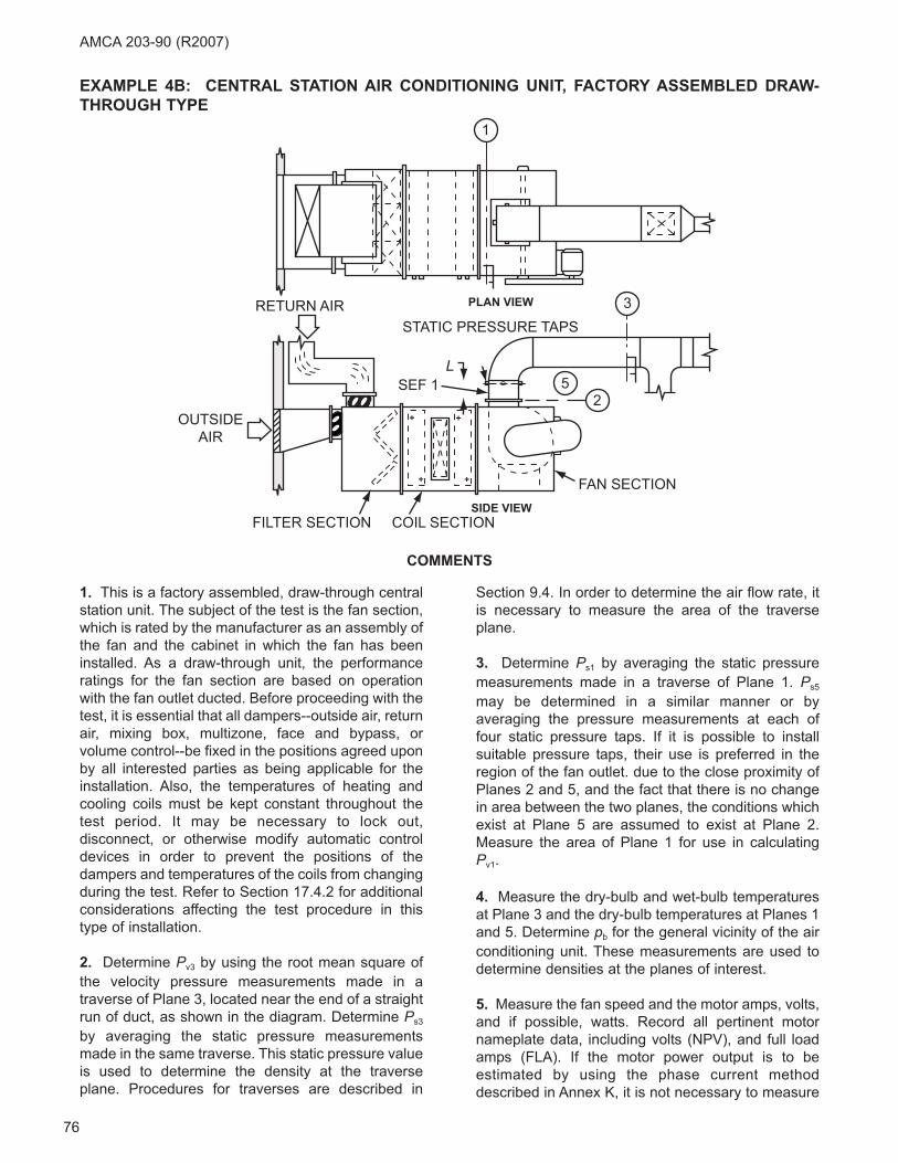
76
AMCA 203-90 (R2007)
1. This is a factory assembled, draw-through central
station unit. The subject of the test is the fan section,
which is rated by the manufacturer as an assembly of
the fan and the cabinet in which the fan has been
installed. As a draw-through unit, the performance
ratings for the fan section are based on operation
with the fan outlet ducted. Before proceeding with the
test, it is essential that all dampers--outside air, return
air, mixing box, multizone, face and bypass, or
volume control--be fixed in the positions agreed upon
by all interested parties as being applicable for the
installation. Also, the temperatures of heating and
cooling coils must be kept constant throughout the
test period. It may be necessary to lock out,
disconnect, or otherwise modify automatic control
devices in order to prevent the positions of the
dampers and temperatures of the coils from changing
during the test. Refer to Section 17.4.2 for additional
considerations affecting the test procedure in this
type of installation.
2. Determine Pv3 by using the root mean square of
the velocity pressure measurements made in a
traverse of Plane 3, located near the end of a straight
run of duct, as shown in the diagram. Determine Ps3
by averaging the static pressure measurements
made in the same traverse. This static pressure value
is used to determine the density at the traverse
plane. Procedures for traverses are described in
Section 9.4. In order to determine the air flow rate, it
is necessary to measure the area of the traverse
plane.
3. Determine Ps1 by averaging the static pressure
measurements made in a traverse of Plane 1. Ps5
may be determined in a similar manner or by
averaging the pressure measurements at each of
four static pressure taps. If it is possible to install
suitable pressure taps, their use is preferred in the
region of the fan outlet. due to the close proximity of
Planes 2 and 5, and the fact that there is no change
in area between the two planes, the conditions which
exist at Plane 5 are assumed to exist at Plane 2.
Measure the area of Plane 1 for use in calculating
Pv1.
4. Measure the dry-bulb and wet-bulb temperatures
at Plane 3 and the dry-bulb temperatures at Planes 1
and 5. Determine pb for the general vicinity of the air
conditioning unit. These measurements are used to
determine densities at the planes of interest.
5. Measure the fan speed and the motor amps, volts,
and if possible, watts. Record all pertinent motor
nameplate data, including volts (NPV), and full load
amps (FLA). If the motor power output is to be
estimated by using the phase current method
described in Annex K, it is not necessary to measure
COMMENTS
1
PLAN VIEWRETURN AIRSTATIC PRESSURE TAPS
SEF 1
OUTSIDEAIR
FILTER SECTION COIL SECTION
FAN SECTION
3
25
L
SIDE VIEW
+
+ +
+
EXAMPLE 4B: CENTRAL STATION AIR CONDITIONING UNIT, FACTORY ASSEMBLED DRAW-
THROUGH TYPE
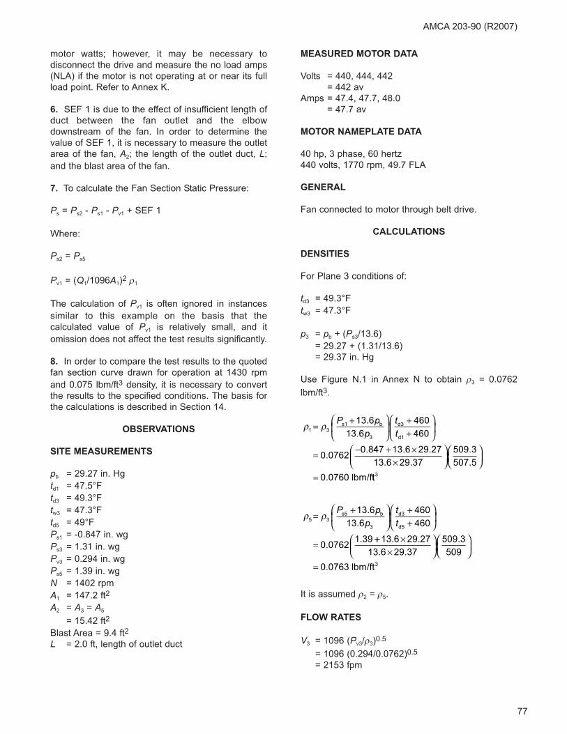
77
motor watts; however, it may be necessary to
disconnect the drive and measure the no load amps
(NLA) if the motor is not operating at or near its full
load point. Refer to Annex K.
6. SEF 1 is due to the effect of insufficient length of
duct between the fan outlet and the elbow
downstream of the fan. In order to determine the
value of SEF 1, it is necessary to measure the outlet
area of the fan, A2; the length of the outlet duct, L;
and the blast area of the fan.
7. To calculate the Fan Section Static Pressure:
Ps = Ps2 - Ps1 - Pv1 + SEF 1
Where:
Ps2 = Ps5
Pv1 = (Q1/1096A1)2 ρ1
The calculation of Pv1 is often ignored in instances
similar to this example on the basis that the
calculated value of Pv1 is relatively small, and it
omission does not affect the test results significantly.
8. In order to compare the test results to the quoted
fan section curve drawn for operation at 1430 rpm
and 0.075 lbm/ft3 density, it is necessary to convert
the results to the specified conditions. The basis for
the calculations is described in Section 14.
OBSERVATIONS
SITE MEASUREMENTS
pb = 29.27 in. Hg
td1 = 47.5°F
td3 = 49.3°F
tw3 = 47.3°F
td5 = 49°F
Ps1 = -0.847 in. wg
Ps3 = 1.31 in. wg
Pv3 = 0.294 in. wg
Ps5 = 1.39 in. wg
N = 1402 rpm
A1 = 147.2 ft2
A2 = A3 = A5
= 15.42 ft2
Blast Area = 9.4 ft2
L = 2.0 ft, length of outlet duct
MEASURED MOTOR DATA
Volts = 440, 444, 442
= 442 av
Amps = 47.4, 47.7, 48.0
= 47.7 av
MOTOR NAMEPLATE DATA
40 hp, 3 phase, 60 hertz
440 volts, 1770 rpm, 49.7 FLA
GENERAL
Fan connected to motor through belt drive.
CALCULATIONS
DENSITIES
For Plane 3 conditions of:
td3 = 49.3°F
tw3 = 47.3°F
p3 = pb + (Ps3/13.6)
= 29.27 + (1.31/13.6)
= 29.37 in. Hg
Use Figure N.1 in Annex N to obtain ρ3 = 0.0762
lbm/ft3.
It is assumed ρ2 = ρ5.
FLOW RATES
V3 = 1096 (Pv3/ρ3)0.5
= 1096 (0.294/0.0762)0.5
= 2153 fpm
ρ ρ5 3
13 6
13 6
460
460
0 07621 39
= +⎛
⎝⎜
⎞
⎠⎟
++
⎛
⎝⎜
⎞
⎠⎟
=
P pp
tt
s5 b
3
d3
d5
.
.
.. ++ ×
×⎛⎝⎜
⎞⎠⎟⎛⎝⎜
⎞⎠⎟
=
13 6 29 27
13 6 29 37
509 3
509
0 0763
. .
. .
.
. lbm/ft3
ρ ρ1 3
13 6
13 6
460
460
0 07620 8
= +⎛
⎝⎜
⎞
⎠⎟
++
⎛
⎝⎜
⎞
⎠⎟
= −
P pp
tt
s1 b
3
d3
d1
.
.
.. 447 13 6 29 27
13 6 29 37
509 3
507 5
0 0760
+ ××
⎛⎝⎜
⎞⎠⎟⎛⎝⎜
⎞⎠⎟
=
. .
. .
.
.
. lbm/ftt3
AMCA 203-90 (R2007)

78
Q3 = V3A3
= 2153 × 15.42
= 33199 cfm
Q = Q1
= Q3 (ρ3/ρ1)
= 33199 (0.0762/0.0760)
= 33286 cfm
Q2 = Q5
= Q3 (ρ3/ρ5)
= 33199 (0.0762/0.0763)
= 33155 cfm
FAN POWER INPUT
Measured amps/FLA = (47.7/49.7)
= 0.96
= 96%
Annex K indicates that Equation A will provide a
reasonably accurate estimate of motor power output
for a 40 hp motor operating at 96% FLA.
Hmo = 40 (47.7/49.7) (442/440)
= 38.6 hp
Figure L.1 in Annex L indicates estimated belt drive
loss of 4.5%.
HL = 0.045 Hmo
= 0.045 × 38.6
= 1.74 hp
H = Hmo - HL
= 38.6 - 1.74
= 36.86 hp
SYSTEM EFFECT FACTOR
To determine SEF 1, AMCA Publication 201-90,
Figures 7.1 and 8.5, indicate the following
calculations:
V2 = (Q2/A2)
= (33155/15.42)
= 2150 fpm
Duct diameter equivalent to the fan outlet area:
De2 = (4 A2/π)0.5
= (4 × 15.42/π)0.5
= 4.43 ft
For velocities of 2500 fpm or less, the 100% effective
outlet duct length is 2.5 duct diameters:
= 2.5 × 4.43
= 11.1 ft
The length of the outlet duct in % effective duct
length:
= (L/11.1) 100
= (2.0/11.1) 100
= 18%
Blast area ratio = Blast Area/A2
= 9.4/15.42
= 0.61
For a blast area ratio of 0.6, 18% effective duct length
and elbow position A, Figure 8.5 shows SystemEffect Curve R applies. For 2150 fpm velocity and
curve R, Figure 7.1 shows SEF 1 = 0.34 in. wg at
0.075 lbm/ft3 density. At 0.0762 lbm/ft3:
SEF 1 = 0.34 (0.0762/0.075)
= 0.35 in. wg
FAN SECTION STATIC PRESSURE
Pv1 = (Q1/1096 A1)2 ρ1
= (33286/1096 × 147.2)2 0.0760
= 0.003 in. wg
It is assumed that Ps2 = Ps5
Ps = Ps2 - Ps1 - Pv1 + SEF 1
= 1.39 - (-0.847) - 0.003 + 0.35
= 2.58 in. wg
CONVERSION TO SPECIFIED CONDITIONS
Qc = 33286 (1430/1402)
= 33951 cfm
Psc = 2.58 (1430/1402)2 (0.075/0.0760)
= 2.65 in. wg
Hc = 36.86 (1430/1402)3 (0.075/0.0760)
= 38.60 hp
AMCA 203-90 (R2007)
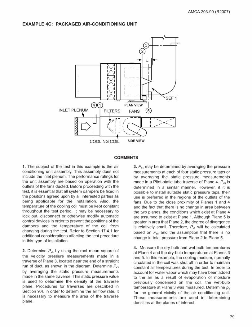
79
AMCA 203-90 (R2007)
1. The subject of the test in this example is the air
conditioning unit assembly. This assembly does not
include the inlet plenum. The performance ratings for
the unit assembly are based on operation with the
outlets of the fans ducted. Before proceeding with the
test, it is essential that all system dampers be fixed in
the positions agreed upon by all interested parties as
being applicable for the installation. Also, the
temperature of the cooling coil must be kept constant
throughout the test period. It may be necessary to
lock out, disconnect or otherwise modify automatic
control devices in order to prevent the positions of the
dampers and the temperature of the coil from
changing during the test. Refer to Section 17.4.1 for
additional considerations affecting the test procedure
in this type of installation.
2. Determine Pv3 by using the root mean square of
the velocity pressure measurements made in a
traverse of Plane 3, located near the end of a straight
run of duct, as shown in the diagram. Determine Ps3
by averaging the static pressure measurements
made in the same traverse. This static pressure value
is used to determine the density at the traverse
plane. Procedures for traverses are described in
Section 9.4. in order to determine the air flow rate, it
is necessary to measure the area of the traverse
plane.
3. Ps4 may be determined by averaging the pressure
measurements at each of four static pressure taps or
by averaging the static pressure measurements
made in a Pitot-static tube traverse of Plane 4. Ps5 is
determined in a similar manner. However, if it is
possible to install suitable static pressure taps, their
use is preferred in the regions of the outlets of the
fans. Due to the close proximity of Planes 1 and 4
and the fact that there is no change in area between
the two planes, the conditions which exist at Plane 4
are assumed to exist at Plane 1. Although Plane 5 is
greater in area that Plane 2, the degree of divergence
is relatively small. Therefore, Ps2 will be calculated
based on Ps5 and the assumption that there is no
change in total pressure from Plane 2 to Plane 5.
4. Measure the dry-bulb and wet-bulb temperatures
at Plane 4 and the dry-bulb temperatures at Planes 3
and 5. In this example, the cooling medium, normally
circulated in the coil was shut off in order to maintain
constant air temperatures during the test. In order to
account for water vapor which may have been added
to the air as a result of evaporation of moisture
previously condensed on the coil, the wet-bulb
temperature at Plane 3 was measured. Determine pb
for the general vicinity of the air conditioning unit.
These measurements are used in determining
densities at the planes of interest.
COMMENTS
23
5
SEF 1
FANSFILTERS
COOLING COIL
INLET PLENUM
L
PLAN VIEW14
SIDE VIEW
+
+
EXAMPLE 4C: PACKAGED AIR-CONDITIONING UNIT

80
5. Measure the fan speed and the motor amps, volts,
and if possible, watts. Record all pertinent motor
nameplate data including volts (NPV), and full load
amps (FLA). If the motor power output is to be
estimated by using the phase current method
described in Annex K, it is not necessary to measure
motor watts; however, it may be necessary to
disconnect the drive and measure the no load amps
(NLA) if the motor is not operating at or near its full
load point. Refer to Annex K.
6. Although an elbow is located shortly downstream
of the fans, SEF 1 is judged to be more closely
characterized as the effect due to insufficient lengths
of duct on the outlets of the fans. In order to
determine the value of SEF 1, it is necessary to
measure the outlet area and the blast area of one of
the fans and the length, L, of its outlet duct.
7. To calculate the static pressure for the unit
assembly:
Ps = Ps2 - Ps1 - Pv1 + SEF 1
Where:
Ps1 = Ps4
Pv1 = (Q1/1096A1)2 ρ1
Ps2 = Ps5 + Pv5 - Pv2
Pv2 and Pv5 are calculated in manners similar to the
calculation of Pv1.
8. In order to compare the test results to the quoted
unit assembly curve drawn for operation at 1050 rpm
and 0.075 lbm/ft3 density, it is necessary to convert
the results to the specified conditions. The basis for
the calculations is described in Section 14.
OBSERVATIONS
SITE MEASUREMENTS
pb = 29.65 in. Hg
td3 = 75.0°F
tw3 = 59.5°F
td4 = 72.5°F
tw4 = 58.5°F
td5 = 74.5°F
Ps3 = 2.02 in. wg
Pv3 = 0.35 in. wg
Ps4 = -0.32 in. wg
Ps5 = 2.11 in. wg
N = 1025 rpm
A1 = A4
= 31.7 ft2
A2 = 11.5 ft2
A3 = 16.4 ft2
A5 = 14.3 ft2
Blast Area = 4.0 ft2 per fan
L = 2.0 ft, length of outlet duct
MEASURED MOTOR DATA
Volts = 460, 455, 465
= 460 av
Amps = 38.2, 38, 37.9
= 38.0 av
MOTOR NAMEPLATE DATA
25 hp, 3 phase, 60 hertz
460 volts, 1760 rpm, 39.5 FLA
GENERAL
Fans connected to motor through belt drive.
CALCULATIONS
DENSITIES
For Plane 3 conditions of:
td3 = 75.0°F
tw3 = 59.5°F
p3 = pb + (Ps3/13.6)
= 29.65 + (2.03/13.6)
= 29.80 in. Hg
Use Figure N.1 in Annex N to obtain ρ3 = 0.0736
lbm/ft3.
For Plane 4 conditions of:
td4 = 72.5°F
tw4 = 58.5°F
p4 = pb + (Ps4/13.5)
= 29.65 + (-0.32/13.6)
= 29.63 in. Hg
Use Figure N.1 in Annex N to obtain ρ4 = 0.0735
lbm/ft3.
It is assumed that ρ1 = ρ4.
AMCA 203-90 (R2007)
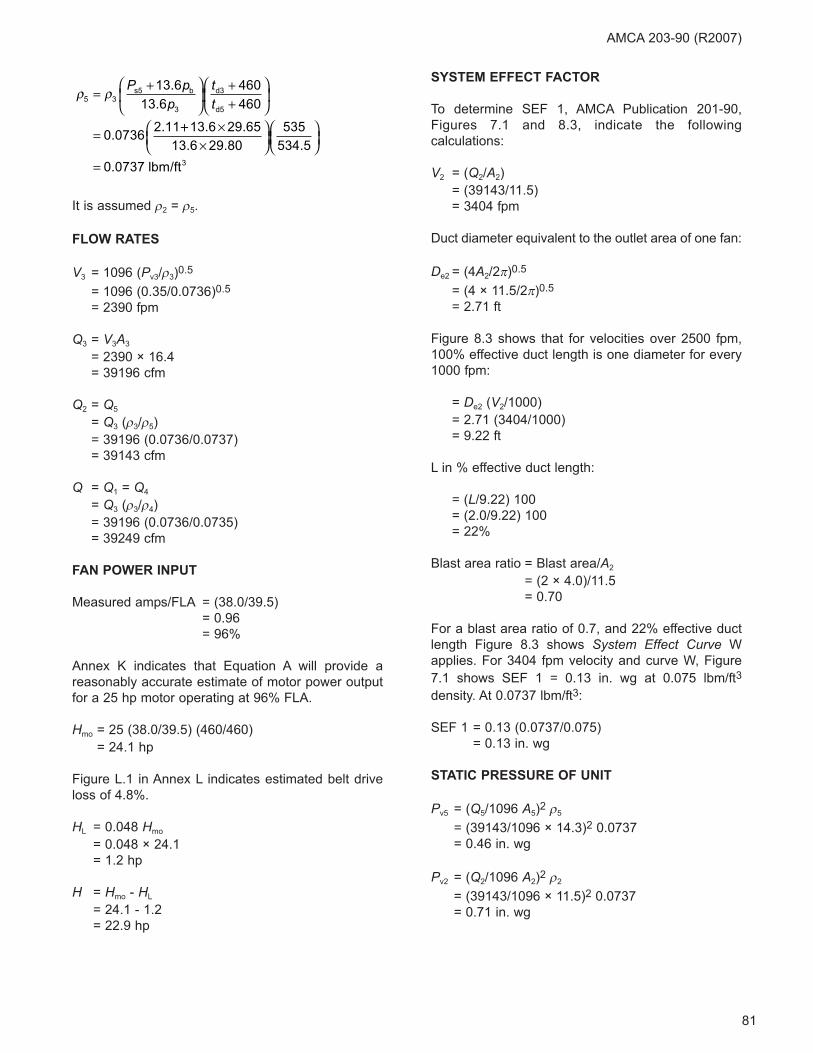
81
It is assumed ρ2 = ρ5.
FLOW RATES
V3 = 1096 (Pv3/ρ3)0.5
= 1096 (0.35/0.0736)0.5
= 2390 fpm
Q3 = V3A3
= 2390 × 16.4
= 39196 cfm
Q2 = Q5
= Q3 (ρ3/ρ5)
= 39196 (0.0736/0.0737)
= 39143 cfm
Q = Q1 = Q4
= Q3 (ρ3/ρ4)
= 39196 (0.0736/0.0735)
= 39249 cfm
FAN POWER INPUT
Measured amps/FLA = (38.0/39.5)
= 0.96
= 96%
Annex K indicates that Equation A will provide a
reasonably accurate estimate of motor power output
for a 25 hp motor operating at 96% FLA.
Hmo = 25 (38.0/39.5) (460/460)
= 24.1 hp
Figure L.1 in Annex L indicates estimated belt drive
loss of 4.8%.
HL = 0.048 Hmo
= 0.048 × 24.1
= 1.2 hp
H = Hmo - HL
= 24.1 - 1.2
= 22.9 hp
SYSTEM EFFECT FACTOR
To determine SEF 1, AMCA Publication 201-90,
Figures 7.1 and 8.3, indicate the following
calculations:
V2 = (Q2/A2)
= (39143/11.5)
= 3404 fpm
Duct diameter equivalent to the outlet area of one fan:
De2 = (4A2/2π)0.5
= (4 × 11.5/2π)0.5
= 2.71 ft
Figure 8.3 shows that for velocities over 2500 fpm,
100% effective duct length is one diameter for every
1000 fpm:
= De2 (V2/1000)
= 2.71 (3404/1000)
= 9.22 ft
L in % effective duct length:
= (L/9.22) 100
= (2.0/9.22) 100
= 22%
Blast area ratio = Blast area/A2
= (2 × 4.0)/11.5
= 0.70
For a blast area ratio of 0.7, and 22% effective duct
length Figure 8.3 shows System Effect Curve W
applies. For 3404 fpm velocity and curve W, Figure
7.1 shows SEF 1 = 0.13 in. wg at 0.075 lbm/ft3
density. At 0.0737 lbm/ft3:
SEF 1 = 0.13 (0.0737/0.075)
= 0.13 in. wg
STATIC PRESSURE OF UNIT
Pv5 = (Q5/1096 A5)2 ρ5
= (39143/1096 × 14.3)2 0.0737
= 0.46 in. wg
Pv2 = (Q2/1096 A2)2 ρ2
= (39143/1096 × 11.5)2 0.0737
= 0.71 in. wg
ρ ρ5 3
3
13 6
13 6
460
460
0 07362 11
= +⎛
⎝⎜
⎞
⎠⎟
++
⎛
⎝⎜
⎞
⎠⎟
=
P pp
tt
s5 b d3
d5
.
.
.. ++ ×
×⎛⎝⎜
⎞⎠⎟⎛⎝⎜
⎞⎠⎟
=
13 6 29 65
13 6 29 80
535
534 5
0 0737
. .
. . .
. lbm/ft3
AMCA 203-90 (R2007)
82
Ps2 + Pv2 = Ps5 + Pv5
Ps2 = Ps5 + Pv5 - Pv2
= 2.11 + 0.46 - 0.71
= 1.86 in. wg
Pv1 = (Q1/1096 A1)2 ρ1
= (39249/1096 × 31.7)2 0.0735
= 0.09 in. wg
Ps = Ps2 - Ps1 - Pv1 + SEF 1
= 1.86 - (-0.32) - 0.09 + 0.13
= 2.22 in. wg
CONVERSION TO SPECIFIED CONDITIONS
Qc = 39249 (1050/1025)
= 40206 cfm
Psc = 2.22 (1050/1025)2 (0.075/0.0735)
= 2.38 in. wg
Hc = 22.9 (1050/1025)3 (0.075/0.0735)
= 25.1 hp
AMCA 203-90 (R2007)

83
AMCA 203-90 (R2007)
1. The subject of the test in this example is the air
conditioning unit assembly. This assembly includes
the filter section and the inlet louver. The
performance ratings for the unit assembly are based
on operation with the outlets of the fans ducted.
Before proceeding with the test, it is essential that all
system dampers be fixed in the positions agreed
upon by all interested parties as being applicable for
the installation. Also, the temperature of the heating
coil must be kept constant throughout the test period.
It may be necessary to lock out, disconnect or
otherwise modify automatic control devices in order
to prevent the positions of the dampers and the
temperature of the coil from changing during the test.
Refer to Section 17.5.1 for additional considerations
affecting the test procedure in this type of installation.
2. Normally, velocity pressure measurements would
be made in a single plane, located in a duct common
to all branches. In this example, a measurement
plane which provides a satisfactory velocity profile
cannot be located upstream of the fans or between
the point of connection of the branch ducts and the
outlets of the fans. The alternative, as indicated in the
diagram, is to make a velocity pressure
measurement traverse in each of two branches. the
velocity pressure for reach branch is determined by
using the root mean square of the velocity pressure
measurements made in the traverse. The static
pressure at each traverse plane is determined by
using the root mean square of the velocity
measurement traverse in each of two branches. The
velocity pressure for each branch is determined by
using the root mean square of the velocity pressure
measurements made in the traverse. The static
pressure at each traverse plane is determined by
averaging the static pressure measurements made in
the same traverse. These static pressure values are
used in determining the densities at the traverse
planes. Procedures for traverses are described in
Section 9.4. In order to determine the air flow rates, it
is necessary to measure the area of each traverse
plane.
3. Determine Ps5 by averaging the pressure
measurements at each of four static pressure taps
located in the duct fitting at the outlets of the fans.
The conditions which exist at Plane 5, including the
static pressure, are assumed to exist at Plane 2,
based on their close proximity and the fact that there
is no change in area between the two planes. In
situations such as this example, it is important to be
certain that all pressure measurements are referred
to the same atmospheric pressure.
4. Measure the dry-bulb and wet-bulb temperatures
at Plane 1 and the dry-bulb temperatures at Planes
3a, 3b, and 5. Determine pb for the general vicinity of
COMMENTS
INLET LOUVER
FILTER SECTION
STATIC PRESSURE TAPS
HEATING COIL
SIDE VIEW
PLAN VIEW
SEF 1
3a
3b
25
1
+ +
L
EXAMPLE 4D: PACKAGED AIR-CONDITIONING UNIT
84
the air conditioning unit. These measurements are
used to determine densities at the planes of interest.
5. Measure the fan speed and the motor amps, volts,
and if possible, watts. Record all pertinent motor
nameplate data, including volts (NPV), and full load
amps (FLA). If the motor power output is to be
estimated by using the phase current method
described in Annex K, it is not necessary to measure
motor watts; however, it may be necessary to
disconnect the drive and measure the no load amps
(NLA) if the motor is not operating at or near its full
load point. Motor performance data, supplied by the
motor manufacturer, are used in the determination of
motor power output in this example.
6. SEF 1 is due to the effect of insufficient length of
duct between the outlets of the fans and the elbow
downstream of the fans. In order to determine the
value of SEF 1, it is necessary to measure the outlet
area and the blast area of one of the fans and the
length of the duct, L, between the fan and the elbow.
7. The sum of the static pressure, Ps1, and velocity
pressure, Pv1, at the inlet to the unit assembly is
considered to be equal to the sum of the static
pressure, Psx, and velocity pressure, Pvx, at a point
sufficiently distant from the inlet as to be in still air. At
this point, the static pressure is zero, and the velocity
pressure in still air is zero.
Ps1 + Pv1 = Psx + Pvx = 0
This consideration, which is the same as that used in
the methods for testing this type of unit for
performance rating purposes, charges to the unit
losses incurred in accelerating the air into its inlet and
eliminates the inaccuracies which arise in any
attempt to measure the velocity pressure and static
pressure at the inlet. To calculate the static pressure
for the unit assembly:
Ps = Ps2 - Ps1 - Pv1 + SEF 1
= Ps2 - (Ps1 + Pv1) + SEF 1
Since:
Ps1 + Pv1 = 0
Ps = Ps2 + SEF 1
Where:
Ps2 = Ps5
8. In order to compare the test results to the quoted
performance curve for the packaged unit drawn for
operation at 1720 rpm and 0.075 lbm/ft3 density, it is
necessary to convert the results to the specified
conditions. The basis for the calculations is described
in Section 14.
OBSERVATIONS
SITE MEASUREMENTS
pb = 29.65 in. Hg
td1 = 72°F
tw1 = 61°F
td5 = 85°F
td3a = 82.5°F
td3b = 83°F
Ps5 = 1.25 in. wg
Ps3a = 1.15 in. wg
Ps3b = 1.22 in. wg
Pv3a = 0.56 in. wg
Pv3b = 0.60 in. wg
N = 1710 rpm
A2 = A5
= 5.64 ft2
A3a = 3.1 ft2
A3b = 2.2 ft2
Blast Area = 2.5 ft2 per fan
L = 0.96 ft, length of outlet duct
MEASURED MOTOR DATA
Volts = 460, 458, 462
= 460 av
Amps = 10.0, 10.0, 9.8
= 9.9 av
MOTOR NAMEPLATE DATA
10 hp, 3 phase, 60 hertz
460 volts, 1750 rpm, 13.5 FLA
GENERAL
Fans connected to motor through belt drive. The
following motor performance data was supplied by
the motor manufacturer:
Motor Efficiency:
82.5% at 1/2 load
84.5% at 3/4 load
84.5% at full load
Power Factor = 0.85
AMCA 203-90 (R2007)

85
DENSITIES
For Plane 1 conditions of:
td1 = 72°F
tw1 = 61°F
p1 = pb
= 29.65 in. Hg
Use Figure N.1 in Annex N to obtain ρ1 = 0.0735
lbm/ft3.
It is assumed that ρ2 = ρ5
FLOW RATES
V3a = 1096 (Pv3a/ρ3a)0.5
= 1096 (0.56/0.0723)0.5
= 3050 fpm
V3b = 1096 (Pv3b/ρ3b)0.5
= 1096 (0.60/0.0722)0.5
= 3159 fpm
Q3a = V3aA3a
= 3050 × 3.1
= 9455 cfm
Q3b = V3bA3b
= 3159 × 2.2
= 6950 cfm
Q = Q1
= Q3a (ρ3a/ρ1) + Q3b (ρ3b/ρ1)
= 9455 (0.0723/0.0735) + 6950 (0.0722/0.0735)
= 16128 cfm
Q2 = Q5
= Q1 (ρ1/ρ5)
= 16128 (0.0735/0.0720)
= 16464 cfm
FAN POWER INPUT
Measured amps/FLA = (9.9/13.5)
= 0.73
= 73%
The data supplied by the motor manufacturer indicate
power factor of 0.85 and motor efficiency of 84.5% for
the motor operating at 73% FLA. Using the
appropriate equation in Section 10.2.2:
Hmo = (3)0.5 × 9.9 × 460 × 0.85 × 0.845/746
= 7.59 hp
Figure L.1 in Annex L indicates estimated belt drive
loss of 5.6%.
HL = 0.056 Hmo
= 0.056 × 7.59
= 0.43 hp
H = Hmo - HL
= 7.59 - 0.43
= 7.16 hp
SYSTEM EFFECT FACTOR
SEF 1 is due to the effect of insufficient lengths of
duct between the outlets of the fans and the elbow
downstream of the fans. AMCA Publication 201-90,
Figures 7.1, 8.1, and 8.5 indicate the following
calculations:
V2 = (Q2/A2)
= (16464/5.64)
= 2919 fpm
Duct diameter equivalent to the outlet area of one
fan:
De2 = (4A2/2π)0.5
= (4 × 5.64/2π)0.5
= 1.89 ft
Figure 8.1 shows that for velocities over 2500 fpm
100% effective duct length is one diameter for every
1000 fpm:
ρ ρ3bs3b b d1
d3b
= +⎛
⎝⎜
⎞
⎠⎟
++
⎛
⎝⎜
⎞
⎠⎟
=
1
1
13 6
13 6
460
460
0 07351
P pp
tt
.
.
... . .
. .
.
22 13 6 29 65
13 6 29 65
532
543
0 0722
+ ××
⎛⎝⎜
⎞⎠⎟⎛⎝⎜
⎞⎠⎟
= lbm/ft3
ρ ρ3as3a b d1
d3a
= +⎛
⎝⎜
⎞
⎠⎟
++
⎛
⎝⎜
⎞
⎠⎟
=
1
1
13 6
13 6
460
460
0 07351
P pp
tt
.
.
... . .
. . .
.
15 13 6 29 65
13 6 29 65
532
542 5
0 0723
+ ××
⎛⎝⎜
⎞⎠⎟⎛⎝⎜
⎞⎠⎟
= lbm/ft33
ρ ρ5 1
1
13 6
13 6
460
460
0 07351 25
= +⎛
⎝⎜
⎞
⎠⎟
++
⎛
⎝⎜
⎞
⎠⎟
=
P pp
tt
s5 b d1
d5
.
.
.. ++ ×
×⎛⎝⎜
⎞⎠⎟⎛⎝⎜
⎞⎠⎟
=
13 6 29 65
13 6 29 65
532
545
0 0720
. .
. .
. lbm/ft3
AMCA 203-90 (R2007)
86
= De2 (V2/1000)
= 1.89 (2919/1000)
= 17%
L, in % effective duct length:
= (L/5.52) 100
= (0.96/5.52) 100
= 17%
Blast area ratio = Blast Area/A2
= (2 × 2.5)/5.64
= 0.89
For a blast area ratio of 0.89, 17% effective duct
length and elbow position C, Figure 8.5 shows
System Effect Curve S applies. For 2919 fpm velocity
and curve S, Figure 7.1 shows SEF 1 = 0.43 in. wg at
0.075 lbm/ft3 density. At 0.0720 lbm/ft3:
SEF 1 = 0.43 (0.0720/0.075)
= 0.41 in. wg
STATIC PRESSURE OF UNIT
Ps2 = Ps5
= 1.25 in. wg
Ps = Ps2 + SEF 1
= 1.25 + 0.41
= 1.66 in. wg
CONVERSION TO SPECIFIED CONDITIONS
Qc = 16128 (1720/1710)
= 16222 cfm
Psc = 1.66 (1720/1710)2 (0.075/0.0735)
= 1.71 in. wg
Hc = 7.16 (1720/1710)3 (0.075/0.0735)
= 7.44 hp
AMCA 203-90 (R2007)
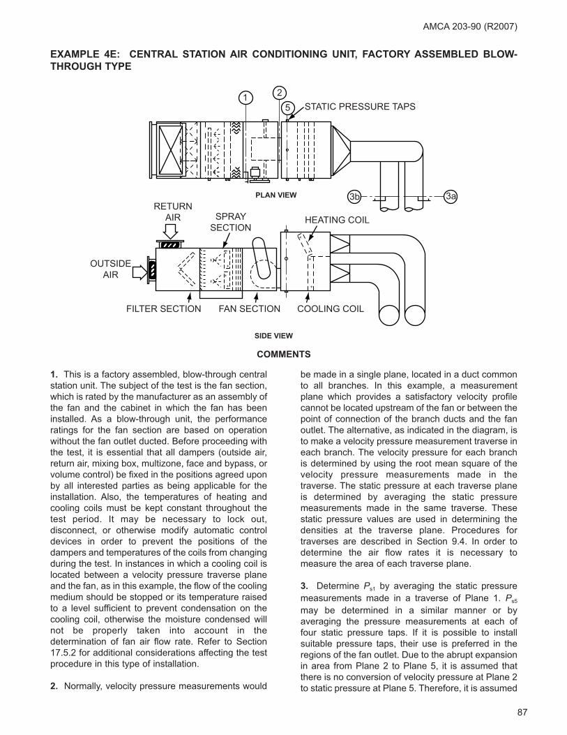
87
AMCA 203-90 (R2007)
1. This is a factory assembled, blow-through central
station unit. The subject of the test is the fan section,
which is rated by the manufacturer as an assembly of
the fan and the cabinet in which the fan has been
installed. As a blow-through unit, the performance
ratings for the fan section are based on operation
without the fan outlet ducted. Before proceeding with
the test, it is essential that all dampers (outside air,
return air, mixing box, multizone, face and bypass, or
volume control) be fixed in the positions agreed upon
by all interested parties as being applicable for the
installation. Also, the temperatures of heating and
cooling coils must be kept constant throughout the
test period. It may be necessary to lock out,
disconnect, or otherwise modify automatic control
devices in order to prevent the positions of the
dampers and temperatures of the coils from changing
during the test. In instances in which a cooling coil is
located between a velocity pressure traverse plane
and the fan, as in this example, the flow of the cooling
medium should be stopped or its temperature raised
to a level sufficient to prevent condensation on the
cooling coil, otherwise the moisture condensed will
not be properly taken into account in the
determination of fan air flow rate. Refer to Section
17.5.2 for additional considerations affecting the test
procedure in this type of installation.
2. Normally, velocity pressure measurements would
be made in a single plane, located in a duct common
to all branches. In this example, a measurement
plane which provides a satisfactory velocity profile
cannot be located upstream of the fan or between the
point of connection of the branch ducts and the fan
outlet. The alternative, as indicated in the diagram, is
to make a velocity pressure measurement traverse in
each branch. The velocity pressure for each branch
is determined by using the root mean square of the
velocity pressure measurements made in the
traverse. The static pressure at each traverse plane
is determined by averaging the static pressure
measurements made in the same traverse. These
static pressure values are used in determining the
densities at the traverse plane. Procedures for
traverses are described in Section 9.4. In order to
determine the air flow rates it is necessary to
measure the area of each traverse plane.
3. Determine Ps1 by averaging the static pressure
measurements made in a traverse of Plane 1. Ps5
may be determined in a similar manner or by
averaging the pressure measurements at each of
four static pressure taps. If it is possible to install
suitable pressure taps, their use is preferred in the
regions of the fan outlet. Due to the abrupt expansion
in area from Plane 2 to Plane 5, it is assumed that
there is no conversion of velocity pressure at Plane 2
to static pressure at Plane 5. Therefore, it is assumed
COMMENTS
1 25
3a3b
STATIC PRESSURE TAPS
HEATING COILSPRAYSECTION
FILTER SECTION FAN SECTION COOLING COIL
RETURNAIR
OUTSIDEAIR
++
+
+
+
+
+
+
SIDE VIEW
PLAN VIEW
EXAMPLE 4E: CENTRAL STATION AIR CONDITIONING UNIT, FACTORY ASSEMBLED BLOW-
THROUGH TYPE
88
that Ps2 = Ps5. Measure the area of Plane 1 for use in
calculating Pv1.
4. Measure the dry-bulb and wet-bulb temperatures
at Planes 1, 3a, and 3b. Determine pb for the general
vicinity of the air conditioning unit. These
measurements are used to determine densities at the
planes of interest. The measurements of additional
wet-bulb temperatures were made in this example in
order to provide data which may be used to
determine whether the moisture content of the air
changed between Plane 1 and Planes 3a and 3b.
5. Measure the fan speed and the motor amps, volts,
and if possible, watts. Record all pertinent motor
nameplate data, including volts (NPV), and full load
amps (FLA). If the motor power output is to be
estimated by using the phase current method
described in Annex K, it is not necessary to measure
motor watts; however, it may be necessary to
disconnect the drive and measure the no load amps
(NLA) if the motor is not operating at or near its full
load point. Refer to Annex K.
6. Since the performance ratings for the fan section
are based on operation without the fan outlet ducted,
an SEF does not apply for the unducted position.
7. To calculate the Fan Section Static Pressure:
Ps = Ps2 - Ps1 - Pv1
Where:
Ps2 = Ps5
Pv1 = (Q1/1096 A1)2 ρ1
Q1 = Q3a (ρ3a/ρ1) + Q3b (ρ3b/ρ1)
The calculation of Pv1 is often ignored in instances
similar to this example on the basis that the
calculated value of Pv1 is relatively small, and its
omission does not affect the test results significantly.
8. In order to compare the test results to the quoted
fan section curve drawn for operation at 1650 rpm
and 0.075 lbm/ft3 density, it is necessary to convert
the results to the specified conditions. The basis for
the calculations is described in Section 14.
OBSERVATIONS
SITE MEASUREMENTS
pb = 28.85 in. Hg
td1 = 65°F
tw1 = 60°F
td3a = 100°F
tw3a = 71.5°F
td3b = 60°F
tw3b = 58°F
Ps1 = -2.43 in. wg
Ps5 = 6.55 in. wg
Ps3a = 5.35 in. wg
Ps3b = 5.1 in. wg
Pv3a = 0.53 in. wg
Pv3b = 0.60 in. wg
N = 1695 rpm
A1 = 68.9 ft2
A3a = 5.37 ft2
A3b = 6.78 ft2
MEASURED MOTOR DATA
Volts = 570, 575, 565
= 570 av
Amps = 81.5, 82.5, 81
= 81.7
NLA = 19
MOTOR NAMEPLATE DATA
100 hp, 3 phase, 60 hertz
575 volts, 1790 rpm, 95 FLA
GENERAL
Fan connected to motor through belt drive.
CALCULATIONS
DENSITIES
For Plane 1 conditions of:
td1 = 65°F
tw1 = 60°F
p1 = pb + (Ps1/13.6)
= 28.85 + (-2.43/13.6)
= 28.67 in. Hg
Use Figure N.1 in Annex N to obtain ρ1 = 0.0720
lbm/ft3.
For Plane 3a conditions of:
td3a = 100°F
tw3a = 71.5°F
p3a = pb + (Ps3a/13.6)
= 28.85 + (5.35/13.6)
= 29.24 in. Hg
AMCA 203-90 (R2007)
89
Use Figure N.1 in Annex N to obtain ρ1 = 0.0720
lbm/ft3.
For Plane 3b conditions of:
td3b = 60°F
tw3b = 58°F
p3b = pb + (Ps3b/13.6)
= 28.85 + (5.1/13.6)
= 29.23 in. Hg
Use Figure N.1 in Annex N to obtain ρ3b = 0.0741
lbm/ft3.
FLOW RATES
V3a = 1096 (Pv3a/ρ3a)0.5
= 1096 (0.53/0.0691)0.5
= 3035 fpm
V3b = 1096 (Pv3b/ρ3b)0.5
= 1096 (0.60/0.0741)0.5
= 3119 fpm
Q3a = V3aA3a
= 3035 × 5.37
= 16298 fpm
Q3b = V3bA3b
= 3119 × 6.78
= 21147 cfm
Q = Q1
= Q3a (ρ3a/ρ1) + Q3b (ρ3b/ρ1)
= 16298 (0.0691/0.0720) + 21147 (0.0741/0.0720)
= 37405 cfm
FAN POWER INPUT
Measured amps/FLA = (81.7/95)
= 0.86
= 86%
Annex K indicates that the average of the results of
Equation A and Equation B will provide a reasonably
accurate estimate of motor power output for a 100 hp
motor operating at 86% of FLA.
Eqn. A = 100 (81.7/95) (570/575)
= 85.3 hp
Eqn. B = 100 [(81.7 - 19)/(95 - 19)] (570/575)
= 81.8 hp
Hmo = (85.3 + 81.8)/2
= 83.6 hp
Reference to Figure L.1 in Annex L indicates
estimated belt drive loss of 4.2%.
HL = 0.042 Hmo
= 0.042 × 83.6
= 3.5 hp
H = Hmo - HL
= 83.6 - 3.5
= 80.1 hp
FAN SECTION STATIC PRESSURE
Pv1 = (Q1/1096 A1)2 ρ1
= (37405/1096 × 68.9)2 0.0720
= 0.02 in. wg
It is assumed that Ps2 = Ps5
Ps = Ps2 - Ps1 - Pv1
= 6.55 - (-2.43) - 0.02
= 8.96 in. wg
CONVERSION TO SPECIFIED CONDITIONS
Qc = 37405 (1650/1695)
= 36412 cfm
Psc = 8.96 (1650/1695)2 (0.075/0.0720)
= 8.84 in. wg
Hc = 80.1 (1650/1695)3 90.075/0.0720)
= 77.0 hp
AMCA 203-90 (R2007)
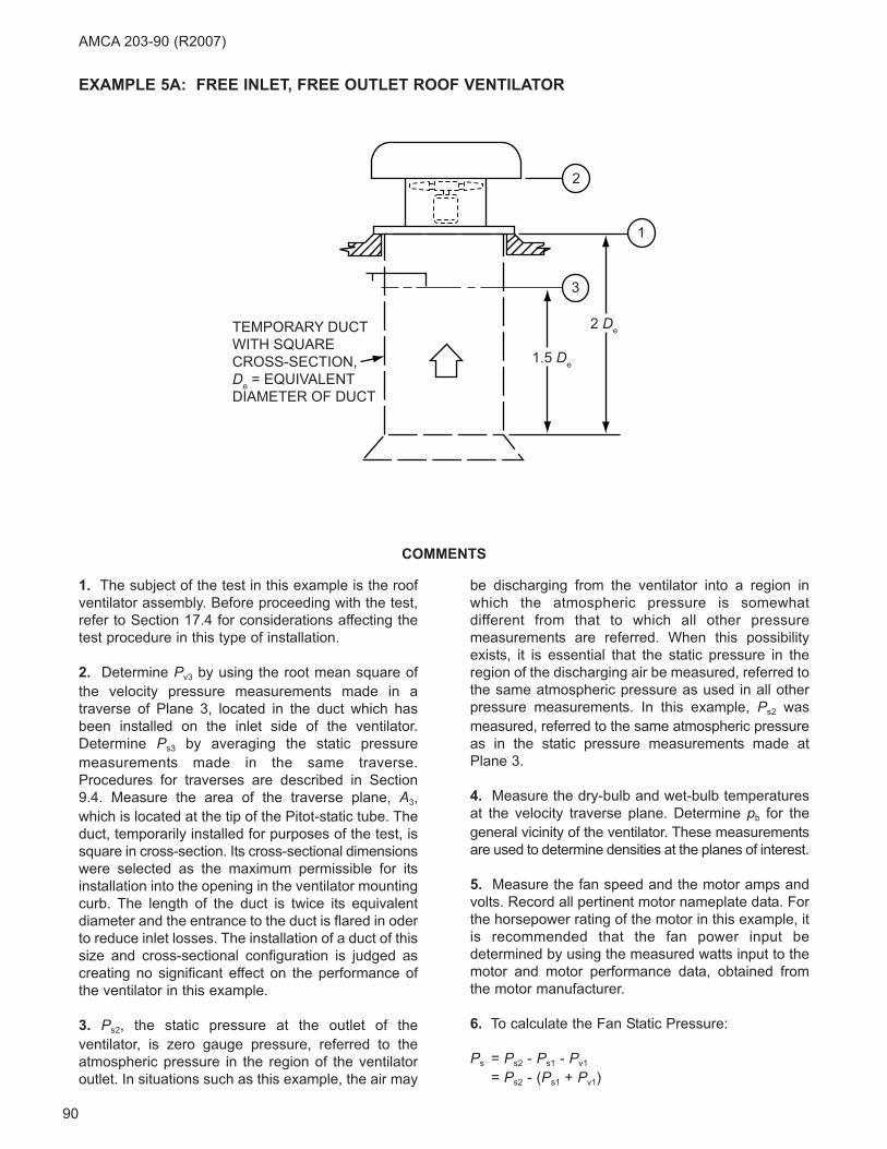
90
AMCA 203-90 (R2007)
1. The subject of the test in this example is the roof
ventilator assembly. Before proceeding with the test,
refer to Section 17.4 for considerations affecting the
test procedure in this type of installation.
2. Determine Pv3 by using the root mean square of
the velocity pressure measurements made in a
traverse of Plane 3, located in the duct which has
been installed on the inlet side of the ventilator.
Determine Ps3 by averaging the static pressure
measurements made in the same traverse.
Procedures for traverses are described in Section
9.4. Measure the area of the traverse plane, A3,
which is located at the tip of the Pitot-static tube. The
duct, temporarily installed for purposes of the test, is
square in cross-section. Its cross-sectional dimensions
were selected as the maximum permissible for its
installation into the opening in the ventilator mounting
curb. The length of the duct is twice its equivalent
diameter and the entrance to the duct is flared in oder
to reduce inlet losses. The installation of a duct of this
size and cross-sectional configuration is judged as
creating no significant effect on the performance of
the ventilator in this example.
3. Ps2, the static pressure at the outlet of the
ventilator, is zero gauge pressure, referred to the
atmospheric pressure in the region of the ventilator
outlet. In situations such as this example, the air may
be discharging from the ventilator into a region in
which the atmospheric pressure is somewhat
different from that to which all other pressure
measurements are referred. When this possibility
exists, it is essential that the static pressure in the
region of the discharging air be measured, referred to
the same atmospheric pressure as used in all other
pressure measurements. In this example, Ps2 was
measured, referred to the same atmospheric pressure
as in the static pressure measurements made at
Plane 3.
4. Measure the dry-bulb and wet-bulb temperatures
at the velocity traverse plane. Determine pb for the
general vicinity of the ventilator. These measurements
are used to determine densities at the planes of interest.
5. Measure the fan speed and the motor amps and
volts. Record all pertinent motor nameplate data. For
the horsepower rating of the motor in this example, it
is recommended that the fan power input be
determined by using the measured watts input to the
motor and motor performance data, obtained from
the motor manufacturer.
6. To calculate the Fan Static Pressure:
Ps = Ps2 - Ps1 - Pv1
= Ps2 - (Ps1 + Pv1)
COMMENTS
2
1
3
TEMPORARY DUCTWITH SQUARECROSS-SECTION,De = EQUIVALENTDIAMETER OF DUCT
1.5 De
2 De
EXAMPLE 5A: FREE INLET, FREE OUTLET ROOF VENTILATOR
91
Where:
Ps1 + Pv1 = Ps3 + Pv3
7. In order to compare the test results to the quoted
fan curve drawn for operation at 1180 rpm and 0.075
lbm/ft3 density, it is necessary to convert the results
to the specified conditions. The basis for the
calculations is described in Section 14.
OBSERVATIONS
SITE MEASUREMENTS
pb = 29.37 in. Hg
td3 = 73.5°F
tw3 = 58.1°F
Ps2 = 0.037 in. wg
Ps3 = -0.085 in. wg
Pv3 = 0.077 in. wg
N = 1177 rpm
A3 = 5.58 ft2
MEASURED MOTOR DATA
Volts = 235, 230, 230
= 232 av
Watts = 755
MOTOR NAMEPLATE DATA
1 hp, 3 phase, 60 hertz
230 volts, 1175 rpm, 3.6 FLA
General
Fan direct connected to motor. Motor efficiency data
supplied by motor manufacturer.
CALCULATIONS
DENSITIES
For Plane 3 conditions of:
td3 = 73.5°F
tw3 = 58.1°F
p3 = pb + (Ps3/13.6)
= 29.37 + (-0.085/13.6)
= 29.36 in. Hg
Use Figure N.1 in Annex N to obtain ρ3 = 0.0727
lbm/ft3.
It is assumed that ρ1 = ρ3.
FLOW RATE
V3 = 1096 (Pv3/ρ3)0.5
= 1096 (0.077/0.0727)0.5
= 1128 fpm
Q = Q1 = Q3
= V3A3
= 1128 × 5.58
= 6294 cfm
FAN POWER INPUT
At the measured power input value of 755 watts, the
data supplied by the motor manufacturer indicate
efficiency of 61% for the motor.
Hmo = (755 × 0.61)/746
= 0.62 hp
Since the fan is direct connected to the motor, there
is no drive loss, and:
H = Hmo
= 0.62 hp
FAN STATIC PRESSURE
Ps1 + Pv1 = Ps3 + Pv3
= -0.085 + 0.077
= -0.008 in. wg
Ps = Ps2 - (Ps1 + Pv1)
= 0.037 - (-0.008)
= 0.045 in. wg
CONVERSION TO SPECIFIED CONDITIONS
Qc = 6294 (1180/1177)
= 6310 cfm
Psc = 0.045 (1180/1177)2 (0.075/0.0727)
= 0.047 in. wg
Hc = 0.62 (1180/1177)3 (0.075/0.0727)
= 0.64 hp
AMCA 203-90 (R2007)
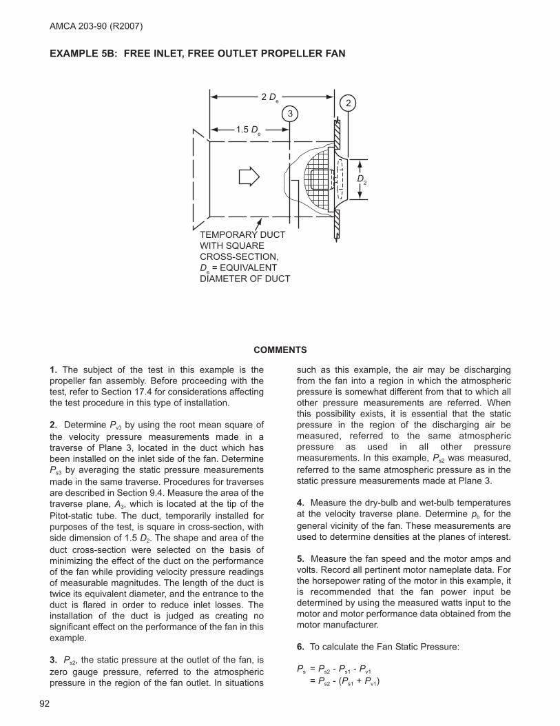
92
AMCA 203-90 (R2007)
1. The subject of the test in this example is the
propeller fan assembly. Before proceeding with the
test, refer to Section 17.4 for considerations affecting
the test procedure in this type of installation.
2. Determine Pv3 by using the root mean square of
the velocity pressure measurements made in a
traverse of Plane 3, located in the duct which has
been installed on the inlet side of the fan. Determine
Ps3 by averaging the static pressure measurements
made in the same traverse. Procedures for traverses
are described in Section 9.4. Measure the area of the
traverse plane, A3, which is located at the tip of the
Pitot-static tube. The duct, temporarily installed for
purposes of the test, is square in cross-section, with
side dimension of 1.5 D2. The shape and area of the
duct cross-section were selected on the basis of
minimizing the effect of the duct on the performance
of the fan while providing velocity pressure readings
of measurable magnitudes. The length of the duct is
twice its equivalent diameter, and the entrance to the
duct is flared in order to reduce inlet losses. The
installation of the duct is judged as creating no
significant effect on the performance of the fan in this
example.
3. Ps2, the static pressure at the outlet of the fan, is
zero gauge pressure, referred to the atmospheric
pressure in the region of the fan outlet. In situations
such as this example, the air may be discharging
from the fan into a region in which the atmospheric
pressure is somewhat different from that to which all
other pressure measurements are referred. When
this possibility exists, it is essential that the static
pressure in the region of the discharging air be
measured, referred to the same atmospheric
pressure as used in all other pressure
measurements. In this example, Ps2 was measured,
referred to the same atmospheric pressure as in the
static pressure measurements made at Plane 3.
4. Measure the dry-bulb and wet-bulb temperatures
at the velocity traverse plane. Determine pb for the
general vicinity of the fan. These measurements are
used to determine densities at the planes of interest.
5. Measure the fan speed and the motor amps and
volts. Record all pertinent motor nameplate data. For
the horsepower rating of the motor in this example, it
is recommended that the fan power input be
determined by using the measured watts input to the
motor and motor performance data obtained from the
motor manufacturer.
6. To calculate the Fan Static Pressure:
Ps = Ps2 - Ps1 - Pv1
= Ps2 - (Ps1 + Pv1)
COMMENTS
32
2 De
1.5 De
TEMPORARY DUCTWITH SQUARECROSS-SECTION,De = EQUIVALENTDIAMETER OF DUCT
D2
EXAMPLE 5B: FREE INLET, FREE OUTLET PROPELLER FAN
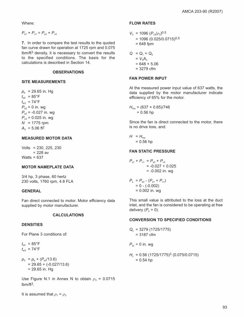
93
Where:
Ps1 + Pv1 = Ps3 + Pv3
7. In order to compare the test results to the quoted
fan curve drawn for operation at 1725 rpm and 0.075
lbm/ft3 density, it is necessary to convert the results
to the specified conditions. The basis for the
calculations is described in Section 14.
OBSERVATIONS
SITE MEASUREMENTS
pb = 29.65 in. Hg
td3 = 85°F
tw3 = 74°F
Ps2 = 0 in. wg
Ps3 = -0.027 in. wg
Pv3 = 0.025 in. wg
N = 1775 rpm
A3 = 5.06 ft2
MEASURED MOTOR DATA
Volts = 230, 225, 230
= 228 av
Watts = 637
MOTOR NAMEPLATE DATA
3/4 hp, 3 phase, 60 hertz
230 volts, 1760 rpm, 4.8 FLA
GENERAL
Fan direct connected to motor. Motor efficiency data
supplied by motor manufacturer.
CALCULATIONS
DENSITIES
For Plane 3 conditions of:
td3 = 85°F
tw3 = 74°F
p3 = pb + (Ps3/13.6)
= 29.65 + (-0.027/13.6)
= 29.65 in. Hg
Use Figure N.1 in Annex N to obtain ρ3 = 0.0715
lbm/ft3.
It is assumed that ρ1 = ρ3
FLOW RATES
V3 = 1096 (Pv3/ρ3)0.5
= 1096 (0.025/0.0715)0.5
= 648 fpm
Q = Q1 = Q3
= V3A3
= 648 × 5.06
= 3279 cfm
FAN POWER INPUT
At the measured power input value of 637 watts, the
data supplied by the motor manufacturer indicate
efficiency of 65% for the motor.
Hmo = (637 × 0.65)/746
= 0.56 hp
Since the fan is direct connected to the motor, there
is no drive loss, and:
H = Hmo
= 0.56 hp
FAN STATIC PRESSURE
Ps1 + Pv1 = Ps3 + Pv3
= -0.027 + 0.025
= -0.002 in. wg
Ps = Ps2 - (Ps1 + Pv1)
= 0 - (-0.002)
= 0.002 in. wg
This small value is attributed to the loss at the duct
inlet, and the fan is considered to be operating at free
delivery (Ps = 0).
CONVERSION TO SPECIFIED CONDITIONS
Qc = 3279 (1725/1775)
= 3187 cfm
Psc = 0 in. wg
Hc = 0.56 (1725/1775)3 (0.075/0.0715)
= 0.54 hp
AMCA 203-90 (R2007)

94
AMCA 203-90 (R2007)
1. The subject of the test in this example is the roof
ventilator assembly. Before proceeding with the test,
refer to Section 17.1 for considerations affecting the
test procedure in this type of installation.
2. Ps3, the static pressure in the vicinity of the
ventilator inlet, would normally be determined by
averaging the static pressure measurements made in
a Pitot tube traverse. But in this example, a
temporary duct was not installed and the Pitot tube
traverse could not be accomplished. In this method
for testing a nonducted fan, consider the fan static
pressure (Ps) as the differential pressure, as read on
a manometer, between the pressure measured inside
the room (Ps3) and the pressure measured outside
the room in the vicinity of the ventilator outlet (Ps2).
These pressures are measured at a sufficient
distance from the ventilator so as to be unaffected by
the velocity of the entering or leaving air.
3. Ps2 is considered to be zero gauge pressure, but
since this measurement is actually part of the
differential pressure described in paragraph 2, it is
necessary to make only one density correction; the
correction is to the differential pressure, which is the
fan static pressure.
4. Measure the dry-bulb and wet-bulb temperatures
in the region of the inside pressure measurement.
Also, determine pb in the same vicinity.
5. Measure the fan speed and the motor amps and
volts. Record all pertinent motor nameplate data. For
the horsepower rating of the motor in this example, it
is recommended that the fan power input be
determined by using the measured watts input to the
motor and motor performance data obtained from the
motor manufacturer.
6. Airflow rates are determined from the fan
manufacturer’s certified performance ratings. Draw a
fan performance curve from these ratings converted
to operation at the test values of fan speed and
entering air density. The basis for these calculations
is described in Section 14. The fan airflow rate is then
determined by entering this curve at the test values of
fan static pressure and fan power input.
OBSERVATIONS
SITE MEASUREMENTS
pb = 29.19 in. Hg
td3 = 79°F
tw3 = 63°F
Ps2 - Ps3 = 0.13 in. wg
N = 1735 rpm
COMMENTS
2
1
3
EXAMPLE 5C: FREE INLET, FREE OUTLET ROOF VENTILATOR

95
MEASURED MOTOR DATA
Volts = 229, 229, 232
= 230 av
Watts = 1390
MOTOR NAMEPLATE DATA
1.5 hp, 3 phase, 60 hertz
230 volts, 1740 rpm, 4.8 FLA
GENERAL
Fan direct connected to motor. Motor efficiency data
supplied by motor manufacturer.
Fan performance, at standard air density, as supplied
by fan manufacturer for 1750 rpm.
CALCULATIONS
DENSITIES
For Plane 3 conditions of:
td3 = 79°F
tw3 = 63°F
pb3 = pb + (Ps2 - Ps1)/13.6
= 29.19 + (0.13/13.6)
= 29.2 in. Hg
Use Figure N.1 in Annex N to obtain ρ3 = 0.0715
lbm/ft3.
It is assumed that ρ1 = ρ3.
FAN POWER INPUT
At the measured power input value of 1395 watts, the
data supplied by the motor manufacturer indicate
efficiency of 77% for the motor.
Hmo = (1390 × 0.77)/746
= 1.43 hp
Since the fan is direct connected to the motor, there
is no drive loss, and:
H = Hmo
= 1.43 hp
FAN STATIC PRESSURE
The fan static pressure is considered to be the
differential static pressure.
Ps = Ps2 - Ps3
= 0.13 in. wg
It is assumed that Ps1 = Ps3
CONVERSION OF MANUFACTURER’S FAN
RATINGS TO OPERATING CONDITIONS
Rating Point #1
Q1c = 8900 (1735/1750)
= 8824 cfm
Ps1c = 0
H1c = 1.45 (1735/1750)3 (0.0715/0.0750)
= 1.35 hp
Rating Point #2
Q2c = 8520 (1735/1750)
= 8447 cfm
Ps2c = 0.125 (1735/1750)2 (0.0715/0.0750)
= 0.117 in. wg
H2c = 1.50 (1735/1750)3 (0.0715/0.0750)
= 1.39 hp
Rating Point #3
Q3c = 8060 (1735/1750)
= 7991 cfm
Ps3c = 0.25 (1735/1750)2 (0.0715/0.0750)
= 0.234 in. wg
H3c = 1.55 (1735/1750)3 (0.0715/0.0750)
= 1.44 hp
Draw a performance curve for these operating
conditions. Enter the measured values for static
pressure and horsepower on the appropriate curves.
Ideally, these two points will coincide at the same
cfm. However, usually they will not coincide and
should be averaged to determine the fan airflow rate.
If this difference is small, such as in this example, it
is only a reflection of test inaccuracies. If, however,
these differences exceed 10%, the system should be
reanalyzed for SEFs that may have been overlooked,
or for procedural errors in the initial testing.
Point CFM Ps HP
1) 8900 0 1.45
2) 8520 1/8 1.50
3) 8060 1/4 1.55
AMCA 203-90 (R2007)

96
AMCA 203-90 (R2007)
Qa = 8070 cfm (based upon horsepower)
Qb = 8400 cfm (based upon static pressure)
Use:
Q = 8235 cfm (average of above).
.40
.30
.20
.10
07000 8000 9000
BH
P (H
)
1.50
1.25
1.00
CFM(Q)
SP
BHP
x
x
x
xx
x
STA
TIC
PR
ES
SU
RE
IN. W
G (P
s)
Fan Performance at 0.0715 Air Density
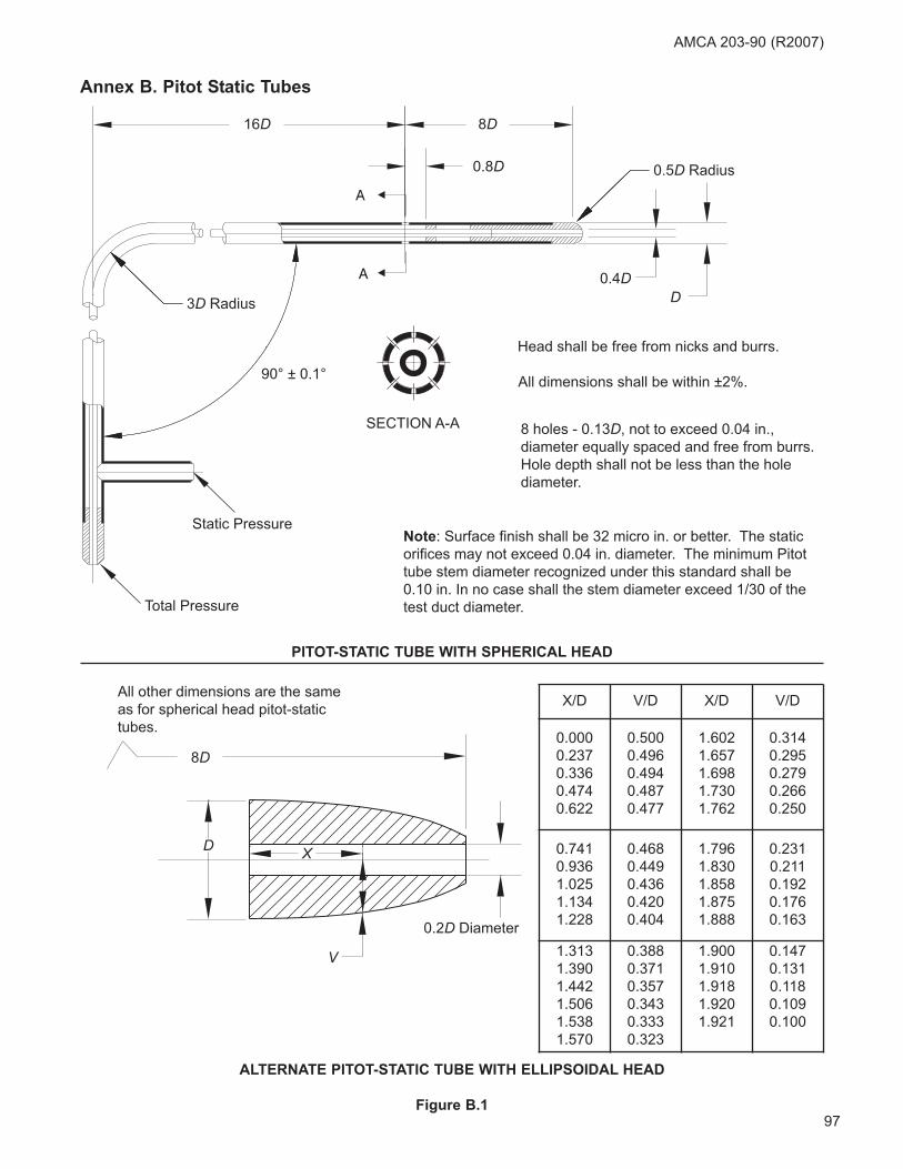
97
AMCA 203-90 (R2007)
Total Pressure
Static Pressure
90° ± 0.1°
3D Radius
SECTION A-A
8D
Head shall be free from nicks and burrs.
All dimensions shall be within ±2%.
Note: Surface finish shall be 32 micro in. or better. The static
orifices may not exceed 0.04 in. diameter. The minimum Pitot
tube stem diameter recognized under this standard shall be
0.10 in. In no case shall the stem diameter exceed 1/30 of the
test duct diameter.
8 holes - 0.13D, not to exceed 0.04 in.,
diameter equally spaced and free from burrs.
Hole depth shall not be less than the hole
diameter.
0.5D Radius
0.4DD
0.8D
16D
All other dimensions are the sameas for spherical head pitot-statictubes.
8D
0.2D Diameter
V
XD
X/D V/D X/D V/D
0.000
0.237
0.336
0.474
0.622
0.500
0.496
0.494
0.487
0.477
1.602
1.657
1.698
1.730
1.762
0.314
0.295
0.279
0.266
0.250
0.741
0.936
1.025
1.134
1.228
0.468
0.449
0.436
0.420
0.404
1.796
1.830
1.858
1.875
1.888
0.231
0.211
0.192
0.176
0.163
1.313
1.390
1.442
1.506
1.538
1.570
0.388
0.371
0.357
0.343
0.333
0.323
1.900
1.910
1.918
1.920
1.921
0.147
0.131
0.118
0.109
0.100
ALTERNATE PITOT-STATIC TUBE WITH ELLIPSOIDAL HEAD
Figure B.1
PITOT-STATIC TUBE WITH SPHERICAL HEAD
Annex B. Pitot Static Tubes
98
AMCA 203-90 (R2007)
READING A
FLEXIBLE TUBINGTOTAL PRESSURE = READING ACORRECTED FOR MANOMETERCALIBRATION
READING B
VELOCITY PRESSURE = READING B CORRECTED FORMANOMETER CALIBRATION ANDCALIBRATION FACTOR FOR THEDOUBLE REVERSE TUBE.
TUBE ENDS MUST BE SMOOTHAND FREE FROM BURRS
REVERSE TUBEIMPACT TUBE
STAINLESS STEELTUBING PREFERREDAPPROX. 0.375 in. OD
SECTION VIEW
AIR FLOW
Notes:
1. For use in dirty or wet gas streams.
2. The double reverse tube must be calibrated and used in the same orientation as used in its calibration
3. Also referred to as impact reverse tube, combined reverse tube, and type S tube.
Figure C.1 - Double Reverse Tube
Annex C. Double Reverse Tubes
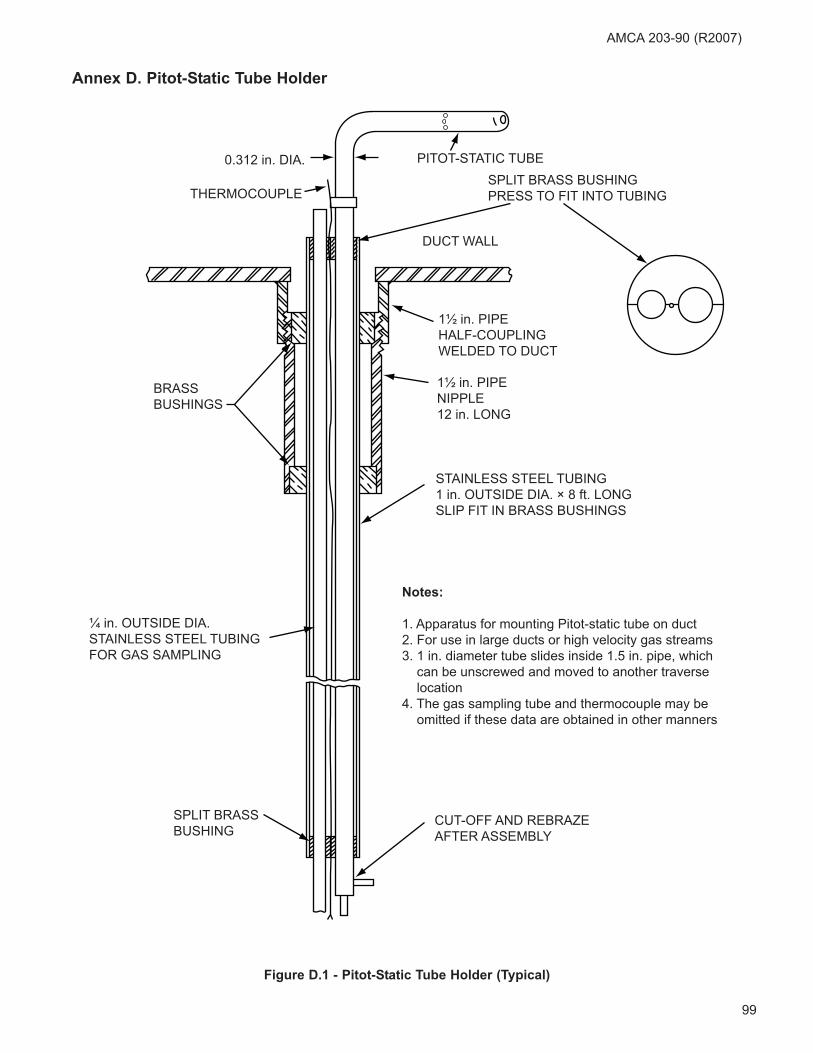
99
AMCA 203-90 (R2007)
Figure D.1 - Pitot-Static Tube Holder (Typical)
PITOT-STATIC TUBESPLIT BRASS BUSHINGPRESS TO FIT INTO TUBING
DUCT WALL
1½ in. PIPENIPPLE12 in. LONG
1½ in. PIPEHALF-COUPLINGWELDED TO DUCT
STAINLESS STEEL TUBING1 in. OUTSIDE DIA. × 8 ft. LONGSLIP FIT IN BRASS BUSHINGS
CUT-OFF AND REBRAZEAFTER ASSEMBLY
SPLIT BRASSBUSHING
¼ in. OUTSIDE DIA.STAINLESS STEEL TUBINGFOR GAS SAMPLING
BRASSBUSHINGS
0.312 in. DIA.
THERMOCOUPLE
Notes:
1. Apparatus for mounting Pitot-static tube on duct2. For use in large ducts or high velocity gas streams3. 1 in. diameter tube slides inside 1.5 in. pipe, which can be unscrewed and moved to another traverse location4. The gas sampling tube and thermocouple may be omitted if these data are obtained in other manners
Annex D. Pitot-Static Tube Holder
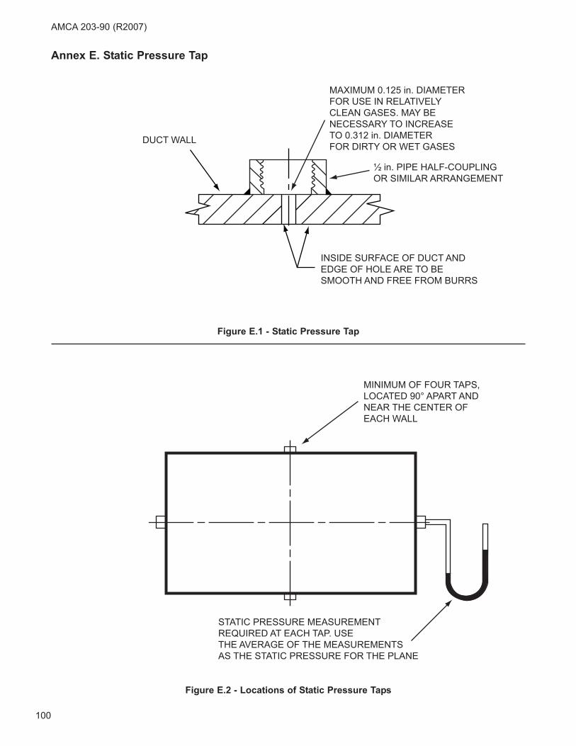
100
AMCA 203-90 (R2007)
DUCT WALL
MAXIMUM 0.125 in. DIAMETERFOR USE IN RELATIVELYCLEAN GASES. MAY BENECESSARY TO INCREASETO 0.312 in. DIAMETERFOR DIRTY OR WET GASES
½ in. PIPE HALF-COUPLINGOR SIMILAR ARRANGEMENT
INSIDE SURFACE OF DUCT ANDEDGE OF HOLE ARE TO BESMOOTH AND FREE FROM BURRS
MINIMUM OF FOUR TAPS,LOCATED 90° APART ANDNEAR THE CENTER OFEACH WALL
STATIC PRESSURE MEASUREMENTREQUIRED AT EACH TAP. USETHE AVERAGE OF THE MEASUREMENTSAS THE STATIC PRESSURE FOR THE PLANE
Figure E.1 - Static Pressure Tap
Figure E.2 - Locations of Static Pressure Taps
Annex E. Static Pressure Tap
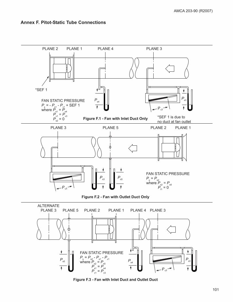
101
AMCA 203-90 (R2007)
Ps3Ps4
Pv3
Ps3
Pv3
Ps3
Pv3
Ps5
PLANE 3PLANE 4PLANE 1PLANE 2
PLANE 3 PLANE 5 PLANE 2 PLANE 1
PLANE 5 PLANE 2 PLANE 1 PLANE 4 PLANE 3
Ps4
*SEF 1
FAN STATIC PRESSUREPs = - Ps1 - Pv1 + SEF 1where Ps1 = Ps4 Pv1 = Pv3 Ps2 = 0
FAN STATIC PRESSUREPs = Ps2 - Ps1 - Pv1where Ps2 = Ps5 Ps1 = Ps4 Pv1 = Pv3
Figure F.1 - Fan with Inlet Duct Only *SEF 1 is due tono duct at fan outlet
FAN STATIC PRESSUREPs = Ps2where Ps2 = Ps5 Pt1 = 0
Figure F.2 - Fan with Outlet Duct Only
Ps5
Figure F.3 - Fan with Inlet Duct and Outlet Duct
ALTERNATEPLANE 3
Annex F. Pitot-Static Tube Connections
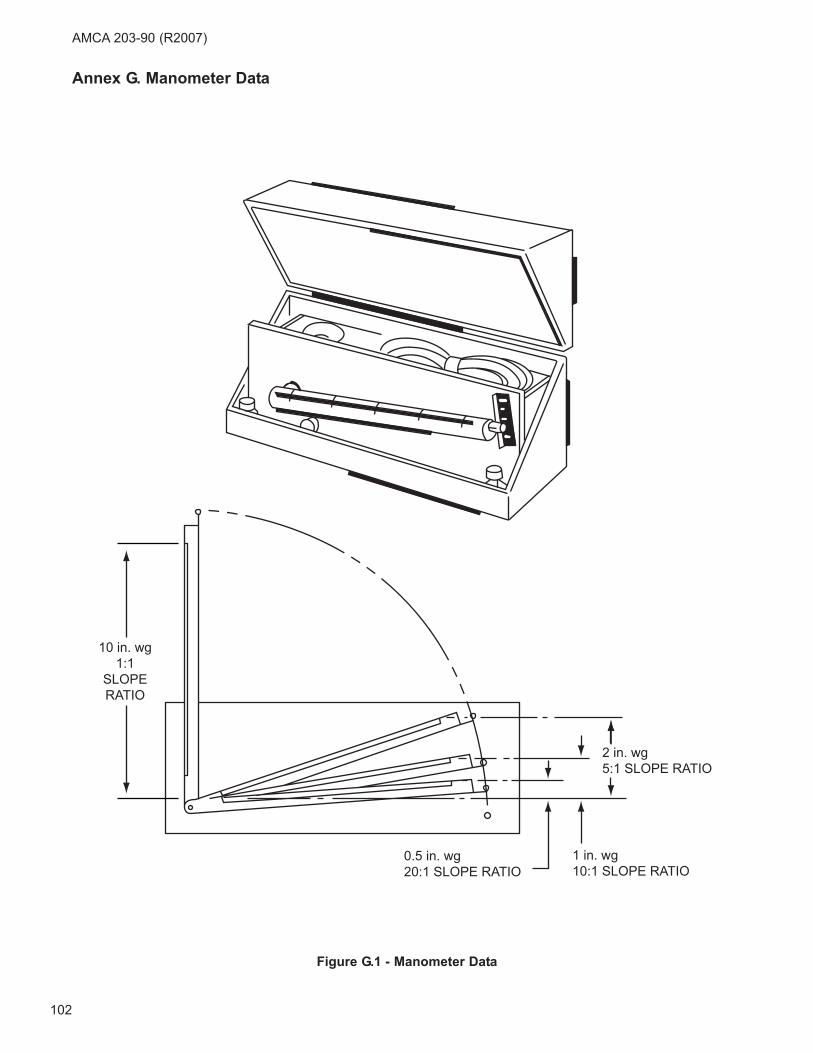
102
AMCA 203-90 (R2007)
Figure G.1 - Manometer Data
0.5 in. wg20:1 SLOPE RATIO
1 in. wg10:1 SLOPE RATIO
2 in. wg5:1 SLOPE RATIO
10 in. wg1:1
SLOPERATIO
Annex G. Manometer Data
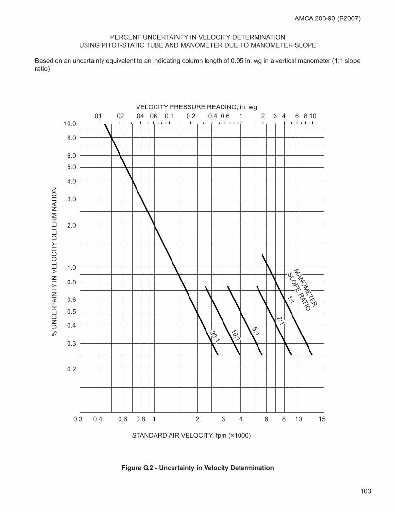
103
AMCA 203-90 (R2007)
VELOCITY PRESSURE READING, in. wg
STANDARD AIR VELOCITY, fpm (×1000)
% U
NC
ER
TAIN
TY IN
VE
LOC
ITY
DE
TER
MIN
ATIO
N
0.3 0.4 0.6 0.8 1 2 3 4 6 8 10 15
0.2
0.3
0.4
0.5
0.6
0.8
1.0
2.0
3.0
4.0
5.0
6.0
8.0
10.0.01 .02 .04 .06 0.1 0.2 0.4 0.6 1 2 3 4 6 8 10
MANO
METER
SLOPE RATIO
20:1
10:1
5:1
2:11:1
Figure G.2 - Uncertainty in Velocity Determination
PERCENT UNCERTAINTY IN VELOCITY DETERMINATION
USING PITOT-STATIC TUBE AND MANOMETER DUE TO MANOMETER SLOPE
Based on an uncertainty equivalent to an indicating column length of 0.05 in. wg in a vertical manometer (1:1 slope
ratio)

104
AMCA 203-90 (R2007)
Figure H.1 - Distribution of Traverse Points for Circular Ducts
INSIDE
DIAMETER
OF DUCT
NUMBER OF
TRAVERSE
POINTS IN
EACH OF 3
DIAMETERS
K1 K2 K3 K4 K5 K6 K7 K8 K9 K10 K11 K12 K13 K14 K15 K16
LESS THAN
8 ft.8 .021 .117 .184 .345 .655 .816 .883 .979
8 ft.
THROUGH
12 ft.
12 .014 .075 .114 .183 .241 .374 .626 .759 .817 .886 .925 .986
GREATER
THAN 12 ft.16 .010 .055 .082 .128 .166 .225 .276 .391 .609 .724 .775 .834 .872 .918 .945 .990
Annex H. Distribution of Traverse Points
In order to obtain a representative average velocity in a duct, it is necessary to locate each traverse point
accurately. It is recommended that the number of traverse points increase with increasing duct size. The
distributions of traverse points for circular ducts, as indicated below, are based on log-linear Pitot traverse method.
D
Xa = D × Ka
Xn
X4
X3
X2X160º
Where:
D is the inside diameter of the duct
Ka is the factor corresponding to the duct size and the traverse point location as indicated in the table below

105
AMCA 203-90 (R2007)
NU
MB
ER
OF
TRAV
ER
SE
PO
INTS
DUCT CROSS-SECTIONAL AREA, ft2
10
15
20
25
30
40
50
60708090
100
10 15 20 25 30 40 50 60 70 80 100 150 200 250 300
Figure H.3 - Recommended Minimum Number
of Traverse Points for Rectangular Ducts
The recommended minimum number of traverse points for rectangular ducts is indicated below in Figure H.3. For
rectangular ducts with cross-sectional areas of 24 square feet and less, the recommended minimum number is 24.
For cross-sectional areas greater than 24 square feet, the minimum number of points increases as indicated in
Figure H.3. The points are to be located in the centers of equal areas with the areas as nearly square as practical
(see Figure H.2). If the flow conditions at the traverse plane are less than satisfactory, the accuracy of the
determination of flow rate may be improved by using more than the recommended minimum number of points.
Fewer points may be used if the flow is very uniform; however, the maximum area covered per point should not
exceed 3 square feet.
X2
Y2
Y
X
Figure H.2 - Distribution of Traverse Points for Rectangular Duct
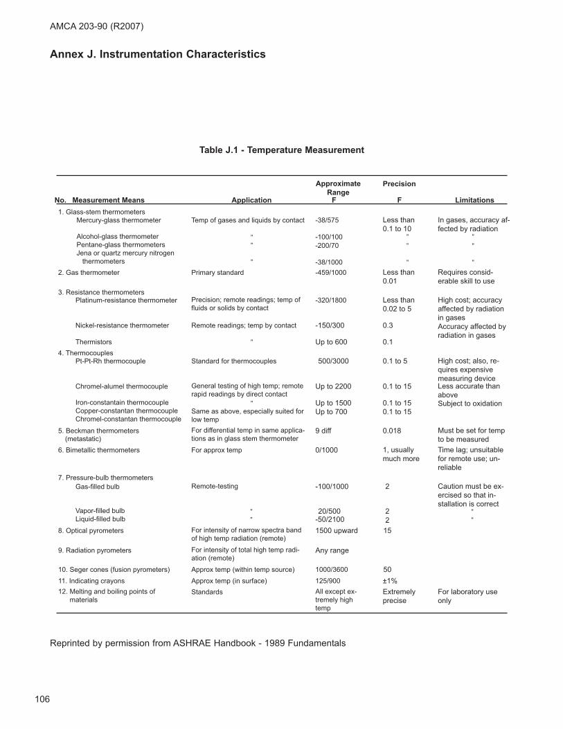
106
AMCA 203-90 (R2007)
1. Glass-stem thermometersMercury-glass thermometer
Alcohol-glass thermometerPentane-glass thermometersJena or quartz mercury nitrogen thermometers
2. Gas thermometer
3. Resistance thermometersPlatinum-resistance thermometer
Nickel-resistance thermometer
Thermistors4. Thermocouples
Temp of gases and liquids by contact
” ” ””
”
””
”
”
”
”
”
”
””
Primary standard
Precision; remote readings; temp offluids or solids by contact
Remote readings; temp by contact
Standard for thermocouples
General testing of high temp; remoterapid readings by direct contact
Same as above, especially suited forlow tempFor differential temp in same applica-tions as in glass stem thermometer
For approx temp
Remote-testing
For intensity of narrow spectra bandof high temp radiation (remote)
For intensity of total high temp radi-ation (remote)Approx temp (within temp source)Approx temp (in surface)Standards
Pt-Pt-Rh thermocouple
Chromel-alumel thermocouple
Iron-constantain thermocoupleCopper-constantan thermocoupleChromel-constantan thermocouple
5. Beckman thermometers(metastatic)
6. Bimetallic thermometers
7. Pressure-bulb thermometersGas-filled bulb
Vapor-filled bulbLiquid-filled bulb
8. Optical pyrometers
9. Radiation pyrometers
10. Seger cones (fusion pyrometers)11. Indicating crayons12. Melting and boiling points of materials
1000/3600125/900All except ex-tremely hightemp
-38/575
-100/100-200/70
-38/1000-459/1000
-320/1800
-150/300
Up to 600
500/3000
Up to 2200
Up to 1500Up to 700
9 diff
0/1000
-100/1000
20/500-50/21001500 upward
Any range
Less than0.1 to 10
Less than0.01
Less than0.02 to 5
0.3
0.1
0.1 to 5
0.1 to 15
0.1 to 150.1 to 15
0.018
1, usuallymuch more
2
22
15
50±1%Extremelyprecise
For laboratory useonly
Limitations
In gases, accuracy af-fected by radiation
Requires consid-erable skill to use
High cost; accuracyaffected by radiationin gasesAccuracy affected byradiation in gases
High cost; also, re-quires expensivemeasuring deviceLess accurate thanaboveSubject to oxidation
Must be set for tempto be measuredTime lag; unsuitablefor remote use; un-reliable
Caution must be ex-ercised so that in-stallation is correct
Precision
FF
ApproximateRange
ApplicationNo. Measurement Means
Reprinted by permission from ASHRAE Handbook - 1989 Fundamentals
Table J.1 - Temperature Measurement
Annex J. Instrumentation Characteristics
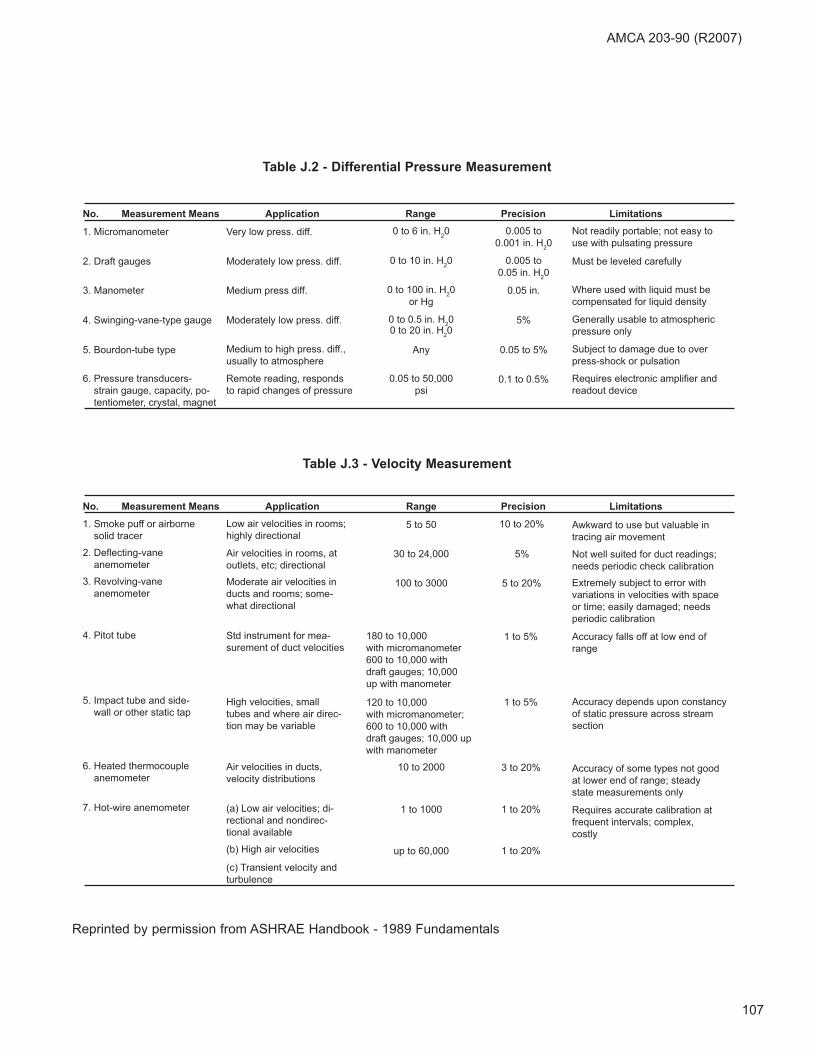
107
AMCA 203-90 (R2007)
1. Micromanometer
2. Draft gauges
3. Manometer
4. Swinging-vane-type gauge
5. Bourdon-tube type
6. Pressure transducers- strain gauge, capacity, po- tentiometer, crystal, magnet
Very low press. diff.
Moderately low press. diff.
Medium press diff.
Moderately low press. diff.
Medium to high press. diff.,usually to atmosphere
Remote reading, respondsto rapid changes of pressure
0 to 6 in. H20
0 to 10 in. H20
0 to 100 in. H20or Hg
0 to 0.5 in. H200 to 20 in. H20
Any
0.05 to 50,000psi
0.005 to0.001 in. H20
0.005 to0.05 in. H20
0.05 in.
5%
0.05 to 5%
0.1 to 0.5%
Not readily portable; not easy touse with pulsating pressure
Must be leveled carefully
Where used with liquid must becompensated for liquid density
Generally usable to atmosphericpressure only
Subject to damage due to overpress-shock or pulsation
Requires electronic amplifier andreadout device
No. Measurement Means Application Range Precision Limitations
No. Measurement Means Application Range Precision Limitations
1. Smoke puff or airborne solid tracer
2. Deflecting-vane anemometer
3. Revolving-vane anemometer
4. Pitot tube
5. Impact tube and side- wall or other static tap
6. Heated thermocouple anemometer
7. Hot-wire anemometer
Low air velocities in rooms;highly directional
Air velocities in rooms, atoutlets, etc; directional
Moderate air velocities inducts and rooms; some-what directional
Std instrument for mea-surement of duct velocities
High velocities, smalltubes and where air direc-tion may be variable
Air velocities in ducts,velocity distributions
(a) Low air velocities; di-rectional and nondirec-tional available
(b) High air velocities
(c) Transient velocity andturbulence
5 to 50
30 to 24,000
100 to 3000
180 to 10,000with micromanometer600 to 10,000 withdraft gauges; 10,000up with manometer
120 to 10,000with micromanometer;600 to 10,000 withdraft gauges; 10,000 upwith manometer
10 to 2000
1 to 1000
up to 60,000
Awkward to use but valuable intracing air movement
Not well suited for duct readings;needs periodic check calibration
Extremely subject to error withvariations in velocities with spaceor time; easily damaged; needsperiodic calibration
Accuracy falls off at low end ofrange
Accuracy depends upon constancyof static pressure across streamsection
Accuracy of some types not goodat lower end of range; steadystate measurements only
Requires accurate calibration atfrequent intervals; complex,costly
10 to 20%
5%
5 to 20%
1 to 5%
1 to 5%
3 to 20%
1 to 20%
1 to 20%
Reprinted by permission from ASHRAE Handbook - 1989 Fundamentals
Table J.2 - Differential Pressure Measurement
Table J.3 - Velocity Measurement
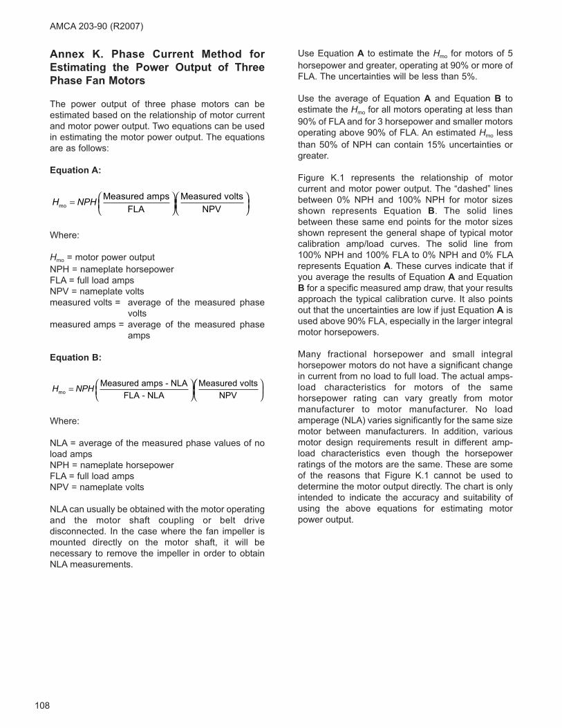
108
Annex K. Phase Current Method for
Estimating the Power Output of Three
Phase Fan Motors
The power output of three phase motors can be
estimated based on the relationship of motor current
and motor power output. Two equations can be used
in estimating the motor power output. The equations
are as follows:
Equation A:
Where:
Hmo = motor power output
NPH = nameplate horsepower
FLA = full load amps
NPV = nameplate volts
measured volts = average of the measured phase
volts
measured amps = average of the measured phase
amps
Equation B:
Where:
NLA = average of the measured phase values of no
load amps
NPH = nameplate horsepower
FLA = full load amps
NPV = nameplate volts
NLA can usually be obtained with the motor operating
and the motor shaft coupling or belt drive
disconnected. In the case where the fan impeller is
mounted directly on the motor shaft, it will be
necessary to remove the impeller in order to obtain
NLA measurements.
Use Equation A to estimate the Hmo for motors of 5
horsepower and greater, operating at 90% or more of
FLA. The uncertainties will be less than 5%.
Use the average of Equation A and Equation B to
estimate the Hmo for all motors operating at less than
90% of FLA and for 3 horsepower and smaller motors
operating above 90% of FLA. An estimated Hmo less
than 50% of NPH can contain 15% uncertainties or
greater.
Figure K.1 represents the relationship of motor
current and motor power output. The “dashed” lines
between 0% NPH and 100% NPH for motor sizes
shown represents Equation B. The solid lines
between these same end points for the motor sizes
shown represent the general shape of typical motor
calibration amp/load curves. The solid line from
100% NPH and 100% FLA to 0% NPH and 0% FLA
represents Equation A. These curves indicate that if
you average the results of Equation A and Equation
B for a specific measured amp draw, that your results
approach the typical calibration curve. It also points
out that the uncertainties are low if just Equation A is
used above 90% FLA, especially in the larger integral
motor horsepowers.
Many fractional horsepower and small integral
horsepower motors do not have a significant change
in current from no load to full load. The actual amps-
load characteristics for motors of the same
horsepower rating can vary greatly from motor
manufacturer to motor manufacturer. No load
amperage (NLA) varies significantly for the same size
motor between manufacturers. In addition, various
motor design requirements result in different amp-
load characteristics even though the horsepower
ratings of the motors are the same. These are some
of the reasons that Figure K.1 cannot be used to
determine the motor output directly. The chart is only
intended to indicate the accuracy and suitability of
using the above equations for estimating motor
power output.
H NPHmo
Measured amps - NLA
FLA - NLA
Measured volts
NPV= ⎛
⎝⎜⎞⎠⎟⎛⎛⎝⎜
⎞⎠⎟
H NPHmo
Measured amps
FLA
Measured volts
NPV= ⎛
⎝⎜⎞⎠⎟⎛⎝⎜
⎞⎠⎟
AMCA 203-90 (R2007)

109
AMCA 203-90 (R2007)
100
90
80
70
60
50
40
30
20
10
00 10 20 30 40 50 60 70 80 90 100
RATEDHORSEPOWER
% NAMEPLATE HORSEPOWER
MEASURED AMPSFLA
3
5
400
10
2500
12
GENERALIZED CURVES ILLUSTRATING THE RELATIONSHIP OF
HORSEPOWER TO AMPS FOR THREE PHASE MOTORS
Do not use for determining actual motor horsepower
DOTTED LINES PER EQUATION B: Hmo ∝ MEASURED AMPS - NLA/FLA - NLA
CAUTION: THIS CHART IS REPRESENTATIVE ONLY! SINCE THE AMP-LOAD CHARACTERISTICS OF THE
SAME SIZE MOTOR WILL VARY BETWEEN THE VARIOUS MOTOR MANUFACTURERS, IT CANNOT BE USED
TO DETERMINE THE HORSEPOWER OUTPUT OF A MOTOR. USE THE EQUATIONS AS DIRECTED ON THE
PREVIOUS PAGE.
PER EQUATION A: Hmo ∝

110
Annex L. Estimated Belt Drive Loss
Drive loss is defined as follows:
Percent drive loss equals power to driving sheave
minus power from driven sheaves times 100, divided
by power to driving sheave.
There are several things which can affect belt drive
efficiencies. Some of these are:
1) Over-designed drives. This was considered good
practice at one time because the drive would last
longer. It will still last longer but it is more
inefficient.
2) Multiple belts on subminimum diameter sheaves
are less efficient than fewer belts on larger
diameter sheaves. Both the National Electric
Motor Association and the Rubber
Manufacturer’s Association publish data dealing
with minimum recommended sheave diameters.
As these minimum sheave diameters are
approached, the drive loss becomes greater.
3) A larger belt section than required will increase
the drive loss.
4) A badly undertensioned drive will increase the
drive loss.
5) Misaligned drives will increase the drive loss.
Drive loss is manifested as heat in belt drives. Under
ambient conditions of less than 100°F, well designed
drives that operate efficiently will be warm to the
touch immediately after being shut down. If the drive
is uncomfortable to the touch (approximately 140°F
or more), then the drive loss is high. Obviously poorly
tensioned and misaligned drives should be corrected
before estimating brake horsepowers and drive
losses.
AMCA 203-90 (R2007)

111
AMCA 203-90 (R2007)
RANGE OF DRIVE LOSSES FOR STANDARD BELTS
MOTOR POWER OUTPUT, hp
DR
IVE
LO
SS
, % M
OTO
R P
OW
ER
OU
TPU
T*
1
1.5
2
3
4
6
8
10
15
20
30
40
60
80
100
0.3 0.4 0.6 0.8 1 2 3 4 6 8 10 20 30 40 60 80 100 200 300 400 600
HIGHER BELT SPEEDS TEND TO HAVE HIGHER LOSSES
THAN LOWER BELT SPEEDS AT THE SAME HORSEPOWER
*Drive losses are based on the conventional V-belt, which has been the “work horse” of the drive industry for
several decades.
EXAMPLE
• Motor power output, Hmo, is determined to be 13.3 hp
• The belts are the standard type and just warm to the touch immediately after shutdown
• From chart, drive loss = 5.1%
• Drive loss, HL = 0.051 × 13.3
= 0.7 hp
• Fan power input, H = 13.3 - 0.7
= 12.6 hp
Figure L.1 - Estimated Belt Drive Loss

112
Annex M. Density Determinations
M.1 General
This annex contains examples illlustrating the
procedures for determining densities. Determinations
of densities are shown for air and for gases other
than air.
M.2 Determination of the density of air,
general case
Determine air density by using the Psychrometric
Density Chart, shown in Figure N.1 in Annex N, the
Psychrometric Density Table, shown in Annex N, or a
calculation procedure which makes use of perfect
gas relationships and the modified Apjohn equation
for partial vapor pressure. Examples of the use of
these procedures are included in this section. Each
of the procedures requires knowledge of the
pressure, dry-bulb temperature and wet-bulb
temperature of the air.
The Psychrometric Density Chart and the
Psychrometric Density Table are limited to the
temperatures and pressures normally encountered in
fan applications.
Limit the use of the calculation procedure that is
based on perfect gas relationships and illustrated in
Example M2.3, to instances in which the dry-bulb
temperature is 180°F or less. Accurate wet-bulb
temperature measurements are difficult to obtain
when the dry-bulb temperature exceeds 180°F.
When the dry-bulb temperature exceeds 180°F, it
may be necessary to rely on site personnel for the
water vapor content of the air. Alternately,
commercially available instrumentation for dew point
determination may be used. For the procedure
required to determine density based on the data
provided in either of the above cases, refer to
Psychrometric Tables and Charts by Zimmerman and
Lavine.1
EXAMPLE M2.1
The conditions that exist at the inlet of a fan that is
not ducted on the inlet side are:
td1 = 78°F
tw1 = 62°F
Since:
Ps1 = 0
p1 = pb
= 28.60 in. Hg
The wet-bulb depression is:
td1 - tw1 = 78 - 62
= 16°F
For wet-bulb depression of 16°F, dry-bulb
temperature of 78°F and absolute pressure of 28.60
in. Hg, obtain ρ1 = 0.0701 lbm/ft3 by using the
Psychrometric Density Chart in Figure N.1 in Annex N.
EXAMPLE M2.2
The conditions at a fan inlet, located at an elevation
of 1000 ft above sea level are:
Ps1 = -3.45 in. wg
td1 = 85°F
tw1 = 75°F
Barometric pressure, obtained from a nearby airport,
is 29.82 in. Hg at sea level.
Using the data in Figure N.3 in Annex N, the
barometric pressure at 1000 ft above sea level is:
pb = 29.82 × 0.964
= 28.75 in. Hg
The absolute pressure at the fan inlet is:
p1 = pb + (Ps1/13.6)
= 28.75 + (-3.45/13.6)
= 28.50 in. Hg
The wet-bulb depression is:
td1 - tw1 = 85 - 75
= 10°F
For dry-bulb temperature of 85°F, absolute pressure
of 28.50 in. Hg and wet-bulb depression of 10°F, use
the Psychrometric Density Table in Figures N.5 in
Annex N to obtain:
ρ1 = 0.06829 + 10 × 0.000041
= 0.0687 lbm/ft3
Example M2.3
The conditions at a fan inlet are:
Ps1 = -8.75 in. wg
td1 = 146°F
tw1 = 93°F
AMCA 203-90 (R2007)
1. O. T. Zimmerman and I. Lavine, Psychrometric Tables and Charts, 2nd ed. (Dover, N.H.: Industrial Research Service Inc., 1964)
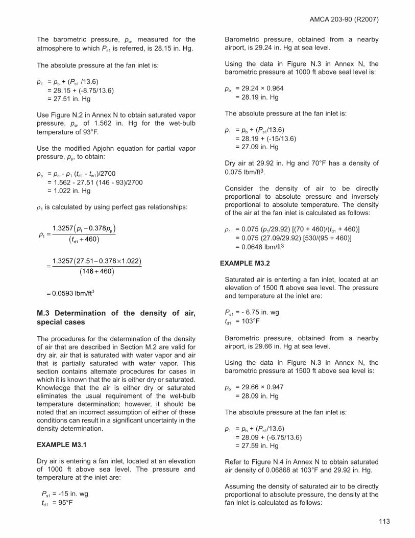
113
The barometric pressure, pb, measured for the
atmosphere to which Ps1 is referred, is 28.15 in. Hg.
The absolute pressure at the fan inlet is:
p1 = pb + (Ps1 /13.6)
= 28.15 + (-8.75/13.6)
= 27.51 in. Hg
Use Figure N.2 in Annex N to obtain saturated vapor
pressure, pe, of 1.562 in. Hg for the wet-bulb
temperature of 93°F.
Use the modified Apjohn equation for partial vapor
pressure, pp, to obtain:
pp = pe - p1 (td1 - tw1)/2700
= 1.562 - 27.51 (146 - 93)/2700
= 1.022 in. Hg
ρ1 is calculated by using perfect gas relationships:
M.3 Determination of the density of air,
special cases
The procedures for the determination of the density
of air that are described in Section M.2 are valid for
dry air, air that is saturated with water vapor and air
that is partially saturated with water vapor. This
section contains alternate procedures for cases in
which it is known that the air is either dry or saturated.
Knowledge that the air is either dry or saturated
eliminates the usual requirement of the wet-bulb
temperature determination; however, it should be
noted that an incorrect assumption of either of these
conditions can result in a significant uncertainty in the
density determination.
EXAMPLE M3.1
Dry air is entering a fan inlet, located at an elevation
of 1000 ft above sea level. The pressure and
temperature at the inlet are:
Ps1 = -15 in. wg
td1 = 95°F
Barometric pressure, obtained from a nearby
airport, is 29.24 in. Hg at sea level.
Using the data in Figure N.3 in Annex N, the
barometric pressure at 1000 ft above seal level is:
pb = 29.24 × 0.964
= 28.19 in. Hg
The absolute pressure at the fan inlet is:
p1 = pb + (Ps1/13.6)
= 28.19 + (-15/13.6)
= 27.09 in. Hg
Dry air at 29.92 in. Hg and 70°F has a density of
0.075 lbm/ft3.
Consider the density of air to be directly
proportional to absolute pressure and inversely
proportional to absolute temperature. The density
of the air at the fan inlet is calculated as follows:
ρ1 = 0.075 (p1/29.92) [(70 + 460)/(td1 + 460)]
= 0.075 (27.09/29.92) [530/(95 + 460)]
= 0.0648 lbm/ft3
EXAMPLE M3.2
Saturated air is enterting a fan inlet, located at an
elevation of 1500 ft above sea level. The pressure
and temperature at the inlet are:
Ps1 = - 6.75 in. wg
td1 = 103°F
Barometric pressure, obtained from a nearby
airport, is 29.66 in. Hg at sea level.
Using the data in Figure N.3 in Annex N, the
barometric pressure at 1500 ft above sea level is:
pb = 29.66 × 0.947
= 28.09 in. Hg
The absolute pressure at the fan inlet is:
p1 = pb + (Ps1/13.6)
= 28.09 + (-6.75/13.6)
= 27.59 in. Hg
Refer to Figure N.4 in Annex N to obtain saturated
air density of 0.06868 at 103°F and 29.92 in. Hg.
Assuming the density of saturated air to be directly
proportional to absolute pressure, the density at the
fan inlet is calculated as follows:
ρ1
11 3257 0 378
460
1 3257 27 51 0 378 1 022
14
=−( )
+( )
=− ×( )
. .
. . . .
p pt
p
d1
66 460
0 0593
+( )
= . lbm/ft3
AMCA 203-90 (R2007)
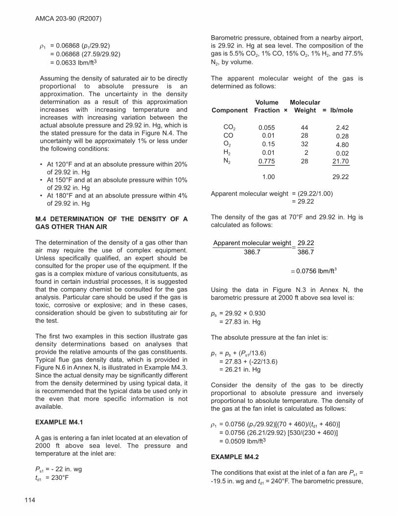
114
AMCA 203-90 (R2007)
ρ1 = 0.06868 (p1/29.92)
= 0.06868 (27.59/29.92)
= 0.0633 lbm/ft3
Assuming the density of saturated air to be directly
proportional to absolute pressure is an
approximation. The uncertainty in the density
determination as a result of this approximation
increases with increasing temperature and
increases with increasing variation between the
actual absolute pressure and 29.92 in. Hg, which is
the stated pressure for the data in Figure N.4. The
uncertainty will be approximately 1% or less under
the following conditions:
• At 120°F and at an absolute pressure within 20%
of 29.92 in. Hg
• At 150°F and at an absolute pressure within 10%
of 29.92 in. Hg
• At 180°F and at an absolute pressure within 4%
of 29.92 in. Hg
M.4 DETERMINATION OF THE DENSITY OF A
GAS OTHER THAN AIR
The determination of the density of a gas other than
air may require the use of complex equipment.
Unless specifically qualified, an expert should be
consulted for the proper use of the equipment. If the
gas is a complex mixture of various consitutuents, as
found in certain industrial processes, it is suggested
that the company chemist be consulted for the gas
analysis. Particular care should be used if the gas is
toxic, corrosive or explosive; and in these cases,
consideration should be given to substituting air for
the test.
The first two examples in this section illustrate gas
density determinations based on analyses that
provide the relative amounts of the gas constituents.
Typical flue gas density data, which is provided in
Figure N.6 in Annex N, is illustrated in Example M4.3.
Since the actual density may be significantly different
from the density determined by using typical data, it
is recommended that the typical data be used only in
the even that more specific information is not
available.
EXAMPLE M4.1
A gas is entering a fan inlet located at an elevation of
2000 ft above sea level. The pressure and
temperature at the inlet are:
Ps1 = - 22 in. wg
td1 = 230°F
Barometric pressure, obtained from a nearby airport,
is 29.92 in. Hg at sea level. The composition of the
gas is 5.5% CO2, 1% CO, 15% O2, 1% H2, and 77.5%
N2, by volume.
The apparent molecular weight of the gas is
determined as follows:
Apparent molecular weight = (29.22/1.00)
= 29.22
The density of the gas at 70°F and 29.92 in. Hg is
calculated as follows:
Using the data in Figure N.3 in Annex N, the
barometric pressure at 2000 ft above sea level is:
pb = 29.92 × 0.930
= 27.83 in. Hg
The absolute pressure at the fan inlet is:
p1 = pb + (Ps1/13.6)
= 27.83 + (-22/13.6)
= 26.21 in. Hg
Consider the density of the gas to be directly
proportional to absolute pressure and inversely
proportional to absolute temperature. The density of
the gas at the fan inlet is calculated as follows:
ρ1 = 0.0756 (p1/29.92)[(70 + 460)/(td1 + 460)]
= 0.0756 (26.21/29.92) [530/(230 + 460)]
= 0.0509 lbm/ft3
EXAMPLE M4.2
The conditions that exist at the inlet of a fan are Ps1 =
-19.5 in. wg and td1 = 240°F. The barometric pressure,
Apparent molecular weight
lbm/ft3
386 7
29 22
386 7
0 0756
.
.
.
.
=
=
Component
Volume
Fraction ×
Molecular
Weight = lb/mole
CO2
CO
O2
H2
N2
0.055
0.01
0.15
0.01
0.775
1.00
44
28
32
2
28
2.42
0.28
4.80
0.02
21.70
29.22

115
AMCA 203-90 (R2007)
pb, measured for the atmospheric to which Ps1 is
referred is 29.35 in. Hg. The composition of the gas
is 5.5% CO2, 1% CO, 15% O2, 1% H2, and 77.5% N2
by weight.
The apparent molecular weight of the gas is
determined as follows:
Apparent molecular weight = 1/0.0390
= 25.6
The density of the gas at 70°F and 29.92 in. Hg is
calculated as follows:
The absolute pressure at the fan inlet is:
p1 = pb + (Ps1/13.6)
= 29.35 + (-19.5/13.6)
= 27.92 in. Hg
Consider the density of the gas to be directly
proportional to absolute pressure and inversely
proportional to absolute temperature. The density of
the gas at the fan inlet is calculated as follows:
ρ1 = 0.0662 (p1/29.92)[(70 + 460)/(td1 + 460)]
= 0.0662 (27.92/29.92) [530/(240 + 460)]
= 0.0468 lbm/ft3
EXAMPLE M4.3
Flue gas is flowing at Plane 3, the Pitot traverse
measurement plane. The flue gas is the result of
using natural gas as the fuel. The conditions that
exsit at Plane 3 are:
Ps3 = 5.74 in. wg
td3 = 680°F
The barometric pressure, pb, measured for the
atmosphere to which Ps3 is referred is 28.85 in. Hg.
The absolute pressure at Plane 3 is:
p3 = pb + (Ps3/13.6)
= 28.85 + (5.74/13.6)
= 29.27 in. Hg
Refer to Figure N.6 in Annex N to obtain typical flue
gas density when natural gas is used as the fuel of
0.0725 lbm/ft3 at 70°F and 29.92 in. Hg.
Consider the density of the flue gas to be directly
proportional to absolute pressure and inversely
proportional to absolute temperature. The density of
the gas at Plane 3 is calculated as follows:
ρ1 = 0.0725 (p3/29.92)[(70 + 460)/(td3 + 460)]
= 0.0725 (29.27/29.92) [530/(680 + 460)]
= 0.0330 lbm/ft3
Apparent molecular weight
lbm/ft3
386 7
25 6
386 7
0 0662
.
.
.
.
=
=
Component
Volume
Fraction ×
Molecular
Weight = lb/mole
CO2
CO
O2
H2
N2
0.055
0.01
0.15
0.01
0.775
1.00
44
28
32
2
28
0.00125
0.00036
0.0047
0.005
0.0277
0.0390

116
AMCA 203-90 (R2007)
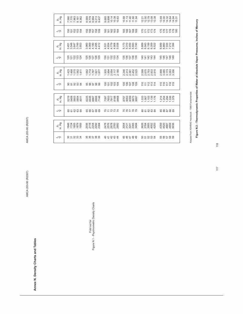
AM
CA
203-9
0 (
R2007)
t w °F
p ein
. H
g
30
31
32
33
34
35
36
37
38
39
40
41
42
43
44
45
46
47
48
49
50
51
52
53
54
55
56
57
58
59
.1646
.1724
.1805
.1879
.1956
.2036
.2118
.2204
.2292
.2384
.2478
.2576
.2678
.2783
.2892
.3004
.3121
.3241
.3365
.3494
.3626
.3764
.3905
.4052
.4203
.4359
.4520
.4687
.4859
.5036
t w °F
p ein
. H
g
60
61
62
63
64
65
66
67
68
69
70
71
72
73
74
75
76
77
78
79
80
81
82
83
84
85
86
87
88
89
.5219
.5408
.5603
.5804
.6011
.6225
.6445
.6667
.6906
.7148
.7397
.7653
.7917
.8188
.8468
.8757
.9053
.9359
.9673
.9997
1.0
33
1.0
67
1.1
03
1.1
39
1.1
76
1.2
14
1.2
54
1.2
94
1.3
36
1.3
79
t w °F
p ein
. H
g
90
91
92
93
94
95
96
97
98
99
100
101
102
103
104
105
106
107
108
109
110
111
112
113
114
115
116
117
118
119
1.4
23
1.4
68
1.5
15
1.5
62
1.6
11
1.6
62
1.7
14
1.7
67
1.8
21
1.8
77
1.9
35
1.9
94
2.0
54
2.1
17
2.1
80
2.2
46
2.3
13
2.3
81
2.4
52
2.5
25
2.5
99
2.6
75
2.7
53
2.8
33
2.9
15
2.9
99
3.0
85
3.1
73
3.2
63
3.3
56
t w °F
p ein
. H
g
120
121
122
123
124
125
126
127
128
129
130
131
132
133
134
135
136
137
138
139
140
141
142
143
144
145
146
147
148
149
3.4
51
3.5
48
3.6
47
3.7
49
3.8
53
3.9
60
4.0
69
4.1
80
4.2
95
4.4
12
4.5
31
4.6
54
4.7
79
4.9
08
5.0
38
5.1
73
5.3
10
5.4
50
5.5
93
5.7
40
5.8
89
6.0
43
6.1
99
6.3
59
6.5
22
6.6
89
6.8
60
7.0
34
7.2
12
7.3
94
t w °F
p ein
. H
g
150
151
152
153
154
155
156
157
158
159
160
161
162
163
164
165
166
167
168
169
170
171
172
173
174
175
176
177
178
179
180
7.5
80
7.7
70
7.9
63
8.1
61
8.3
62
8.5
69
8.7
79
8.9
94
9.2
13
9.4
37
9.6
65
9.8
98
10.1
4
10.3
8
10.6
3
10.8
8
11.1
3
11.4
0
11.6
6
11.9
4
12.2
1
12.5
0
12.7
9
13.0
8
13.3
8
13.6
9
14.0
0
14.3
2
14.6
4
14.9
4
15.3
1
Adapte
d f
rom
AS
HR
AE
Handbook -
1989 F
andam
enta
ls
Fig
ure
N.2
- T
herm
od
yn
am
ic P
rop
ert
ies o
f W
ate
r at
Ab
so
lute
Vap
or
Pre
ssu
res,
Inch
es o
f M
erc
ury
AM
CA
203-9
0 (
R2007)
An
nex N
. D
en
sit
y C
hart
s a
nd
Tab
les
117
118
Fold
out
for
Fig
ure
N.1
- P
sychro
metr
ic D
ensity C
hart
s
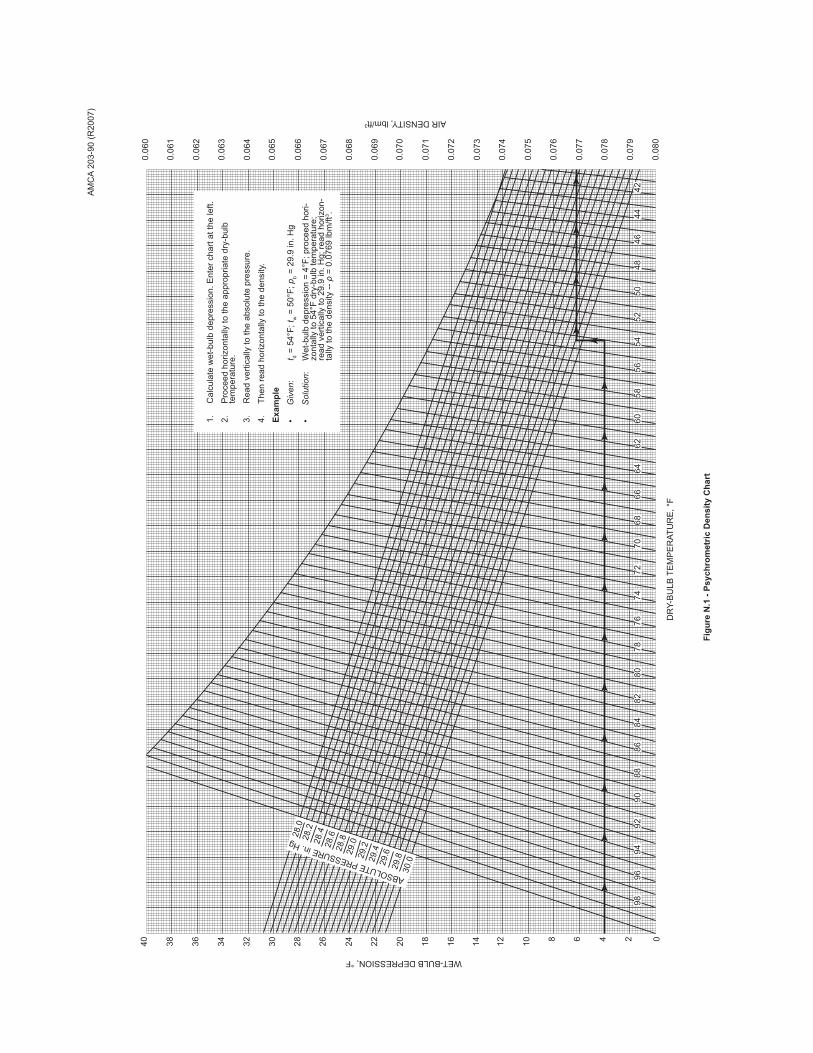
AM
CA
203-9
0 (
R2007)
DR
Y-B
ULB
TE
MP
ER
ATU
RE
, °F
WET-BULB DEPRESSION, °F
AIR DENSITY, lbm/ft3
0.06
0
0.06
1
0.06
2
0.06
3
0.06
4
0.06
5
0.06
6
0.06
7
0.06
8
0.06
9
0.07
0
0.07
1
0.07
2
0.07
3
0.07
4
0.07
5
0.07
6
0.07
7
0.07
8
0.07
9
0.08
00246810121416182022242628303234363840
4244
4648
5052
5456
5860
6264
6668
7072
7476
7880
8284
8688
9092
9496
98
1.
Cal
cula
te w
et-b
ulb
depr
essi
on. E
nter
cha
rt at
the
left.
2.
Pro
ceed
hor
izon
tally
to th
e ap
prop
riate
dry
-bul
b
t
empe
ratu
re.
3.
Rea
d ve
rtica
lly to
the
abso
lute
pre
ssur
e.
4.
The
n re
ad h
oriz
onta
lly to
the
dens
ity.
Exam
ple
•Given
:t d
= 54
°F; t
w =
50°
F; p
b = 2
9.9
in. H
g
•Solution:
W
et-b
ulb
depr
essi
on =
4°F
; pro
ceed
hor
i-
zo
ntal
ly to
54°
F dr
y-bu
lb te
mpe
ratu
re;
read
ver
tical
ly to
29.
9 in
. Hg;
read
hor
izon
-
ta
lly to
the
dens
ity --
ρ =
0.0
769
lbm
/ft3 .
28.0
28.2
28.4
28.6
28.8
29.0
29.2
29.4
29.6
29.8
30.0
ABSOLUTE PRESSURE in. Hg
Fig
ure
N.1
- P
sych
rom
etr
ic D
en
sit
y C
hart
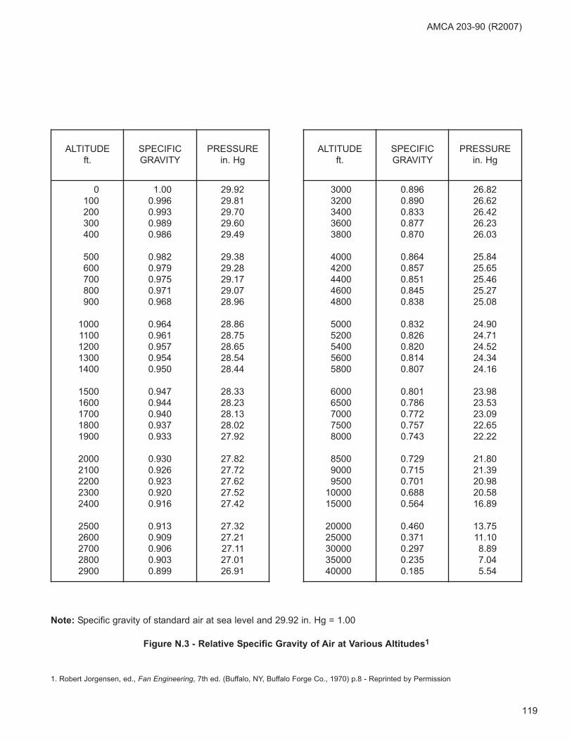
119
AMCA 203-90 (R2007)
ALTITUDE
ft.
SPECIFIC
GRAVITY
PRESSURE
in. Hg
0
100
200
300
400
500
600
700
800
900
1000
1100
1200
1300
1400
1500
1600
1700
1800
1900
2000
2100
2200
2300
2400
2500
2600
2700
2800
2900
1.00
0.996
0.993
0.989
0.986
0.982
0.979
0.975
0.971
0.968
0.964
0.961
0.957
0.954
0.950
0.947
0.944
0.940
0.937
0.933
0.930
0.926
0.923
0.920
0.916
0.913
0.909
0.906
0.903
0.899
29.92
29.81
29.70
29.60
29.49
29.38
29.28
29.17
29.07
28.96
28.86
28.75
28.65
28.54
28.44
28.33
28.23
28.13
28.02
27.92
27.82
27.72
27.62
27.52
27.42
27.32
27.21
27.11
27.01
26.91
ALTITUDE
ft.
SPECIFIC
GRAVITY
PRESSURE
in. Hg
3000
3200
3400
3600
3800
4000
4200
4400
4600
4800
5000
5200
5400
5600
5800
6000
6500
7000
7500
8000
8500
9000
9500
10000
15000
20000
25000
30000
35000
40000
0.896
0.890
0.833
0.877
0.870
0.864
0.857
0.851
0.845
0.838
0.832
0.826
0.820
0.814
0.807
0.801
0.786
0.772
0.757
0.743
0.729
0.715
0.701
0.688
0.564
0.460
0.371
0.297
0.235
0.185
26.82
26.62
26.42
26.23
26.03
25.84
25.65
25.46
25.27
25.08
24.90
24.71
24.52
24.34
24.16
23.98
23.53
23.09
22.65
22.22
21.80
21.39
20.98
20.58
16.89
13.75
11.10
8.89
7.04
5.54
Note: Specific gravity of standard air at sea level and 29.92 in. Hg = 1.00
Figure N.3 - Relative Specific Gravity of Air at Various Altitudes1
1. Robert Jorgensen, ed., Fan Engineering, 7th ed. (Buffalo, NY, Buffalo Forge Co., 1970) p.8 - Reprinted by Permission
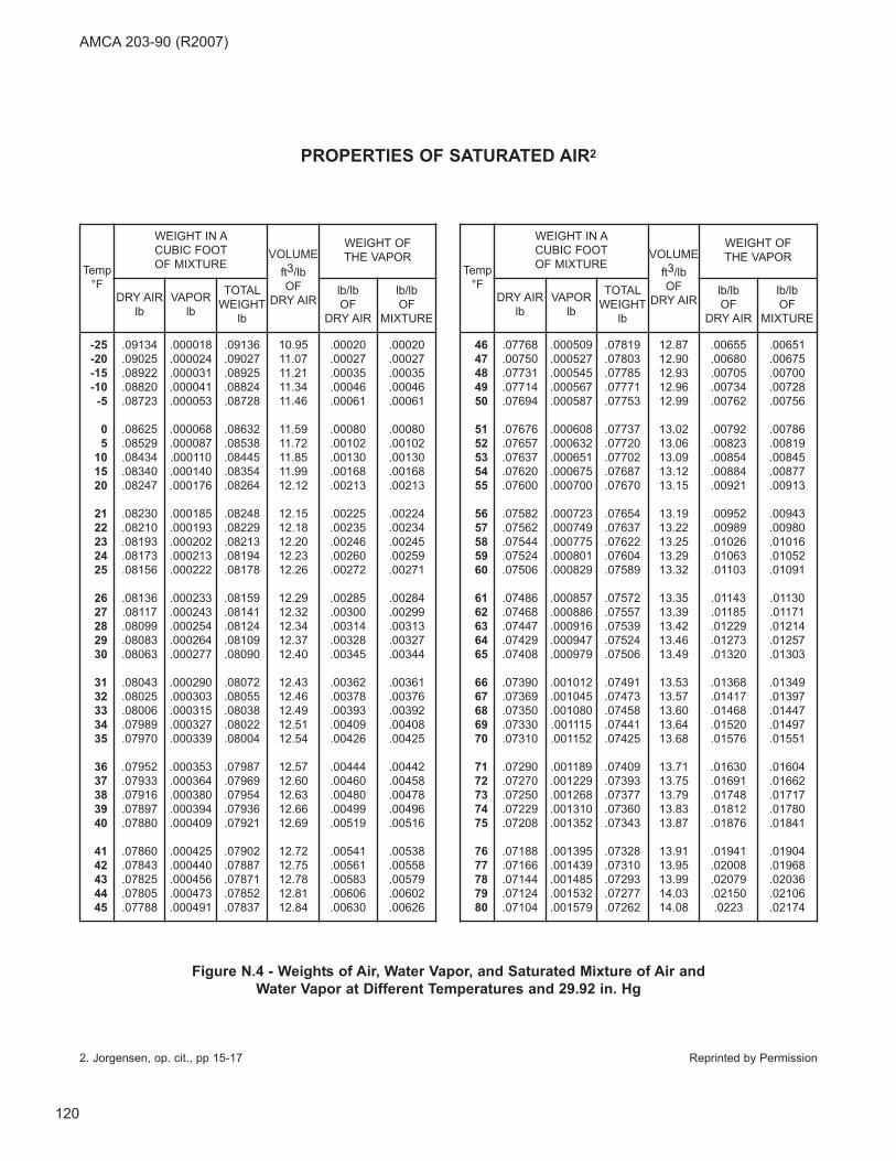
Temp
°F
WEIGHT IN A
CUBIC FOOT
OF MIXTUREVOLUME
ft3/lb
OF
DRY AIR
WEIGHT OF
THE VAPOR
DRY AIR
lb
VAPOR
lb
TOTAL
WEIGHT
lb
lb/lb
OF
DRY AIR
lb/lb
OF
MIXTURE
-25
-20
-15
-10
-5
0
5
10
15
20
21
22
23
24
25
26
27
28
29
30
31
32
33
34
35
36
37
38
39
40
41
42
43
44
45
.09134
.09025
.08922
.08820
.08723
.08625
.08529
.08434
.08340
.08247
.08230
.08210
.08193
.08173
.08156
.08136
.08117
.08099
.08083
.08063
.08043
.08025
.08006
.07989
.07970
.07952
.07933
.07916
.07897
.07880
.07860
.07843
.07825
.07805
.07788
.000018
.000024
.000031
.000041
.000053
.000068
.000087
.000110
.000140
.000176
.000185
.000193
.000202
.000213
.000222
.000233
.000243
.000254
.000264
.000277
.000290
.000303
.000315
.000327
.000339
.000353
.000364
.000380
.000394
.000409
.000425
.000440
.000456
.000473
.000491
.09136
.09027
.08925
.08824
.08728
.08632
.08538
.08445
.08354
.08264
.08248
.08229
.08213
.08194
.08178
.08159
.08141
.08124
.08109
.08090
.08072
.08055
.08038
.08022
.08004
.07987
.07969
.07954
.07936
.07921
.07902
.07887
.07871
.07852
.07837
10.95
11.07
11.21
11.34
11.46
11.59
11.72
11.85
11.99
12.12
12.15
12.18
12.20
12.23
12.26
12.29
12.32
12.34
12.37
12.40
12.43
12.46
12.49
12.51
12.54
12.57
12.60
12.63
12.66
12.69
12.72
12.75
12.78
12.81
12.84
.00020
.00027
.00035
.00046
.00061
.00080
.00102
.00130
.00168
.00213
.00225
.00235
.00246
.00260
.00272
.00285
.00300
.00314
.00328
.00345
.00362
.00378
.00393
.00409
.00426
.00444
.00460
.00480
.00499
.00519
.00541
.00561
.00583
.00606
.00630
.00020
.00027
.00035
.00046
.00061
.00080
.00102
.00130
.00168
.00213
.00224
.00234
.00245
.00259
.00271
.00284
.00299
.00313
.00327
.00344
.00361
.00376
.00392
.00408
.00425
.00442
.00458
.00478
.00496
.00516
.00538
.00558
.00579
.00602
.00626
Temp
°F
WEIGHT IN A
CUBIC FOOT
OF MIXTUREVOLUME
ft3/lb
OF
DRY AIR
WEIGHT OF
THE VAPOR
DRY AIR
lb
VAPOR
lb
TOTAL
WEIGHT
lb
lb/lb
OF
DRY AIR
lb/lb
OF
MIXTURE
46
47
48
49
50
51
52
53
54
55
56
57
58
59
60
61
62
63
64
65
66
67
68
69
70
71
72
73
74
75
76
77
78
79
80
.07768
.00750
.07731
.07714
.07694
.07676
.07657
.07637
.07620
.07600
.07582
.07562
.07544
.07524
.07506
.07486
.07468
.07447
.07429
.07408
.07390
.07369
.07350
.07330
.07310
.07290
.07270
.07250
.07229
.07208
.07188
.07166
.07144
.07124
.07104
.000509
.000527
.000545
.000567
.000587
.000608
.000632
.000651
.000675
.000700
.000723
.000749
.000775
.000801
.000829
.000857
.000886
.000916
.000947
.000979
.001012
.001045
.001080
.001115
.001152
.001189
.001229
.001268
.001310
.001352
.001395
.001439
.001485
.001532
.001579
.07819
.07803
.07785
.07771
.07753
.07737
.07720
.07702
.07687
.07670
.07654
.07637
.07622
.07604
.07589
.07572
.07557
.07539
.07524
.07506
.07491
.07473
.07458
.07441
.07425
.07409
.07393
.07377
.07360
.07343
.07328
.07310
.07293
.07277
.07262
12.87
12.90
12.93
12.96
12.99
13.02
13.06
13.09
13.12
13.15
13.19
13.22
13.25
13.29
13.32
13.35
13.39
13.42
13.46
13.49
13.53
13.57
13.60
13.64
13.68
13.71
13.75
13.79
13.83
13.87
13.91
13.95
13.99
14.03
14.08
.00655
.00680
.00705
.00734
.00762
.00792
.00823
.00854
.00884
.00921
.00952
.00989
.01026
.01063
.01103
.01143
.01185
.01229
.01273
.01320
.01368
.01417
.01468
.01520
.01576
.01630
.01691
.01748
.01812
.01876
.01941
.02008
.02079
.02150
.0223
.00651
.00675
.00700
.00728
.00756
.00786
.00819
.00845
.00877
.00913
.00943
.00980
.01016
.01052
.01091
.01130
.01171
.01214
.01257
.01303
.01349
.01397
.01447
.01497
.01551
.01604
.01662
.01717
.01780
.01841
.01904
.01968
.02036
.02106
.02174
Figure N.4 - Weights of Air, Water Vapor, and Saturated Mixture of Air and
Water Vapor at Different Temperatures and 29.92 in. Hg
2. Jorgensen, op. cit., pp 15-17 Reprinted by Permission
PROPERTIES OF SATURATED AIR2
AMCA 203-90 (R2007)
120
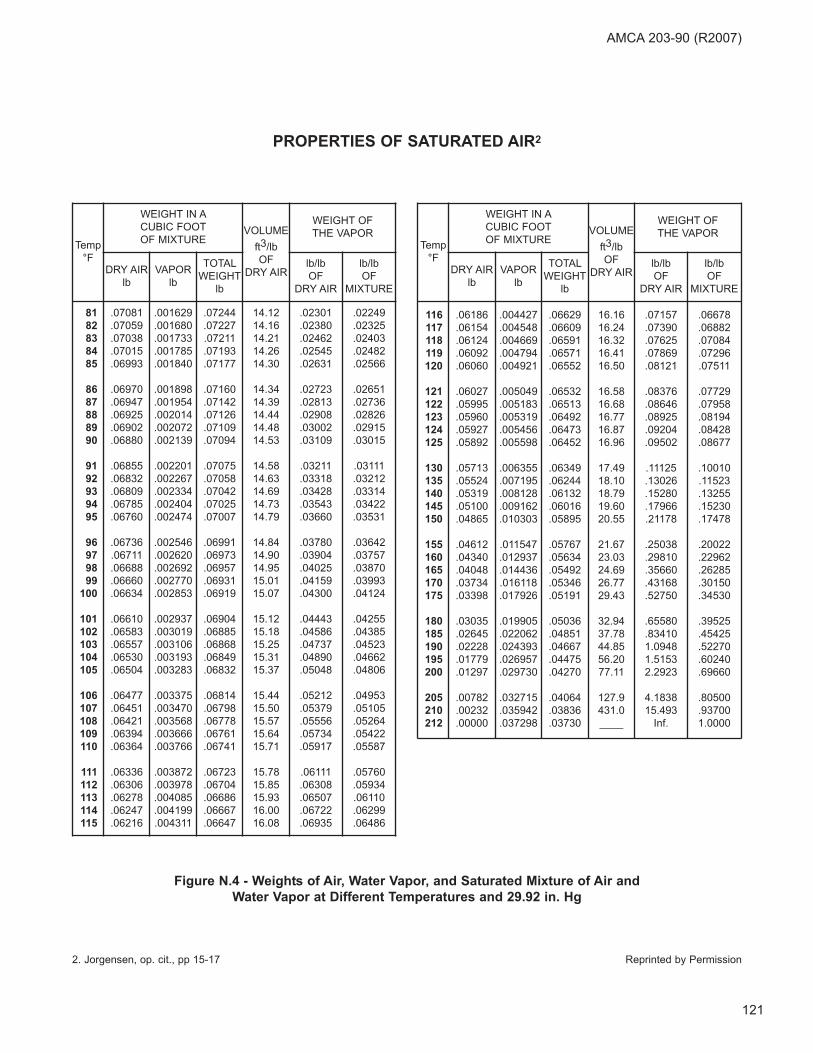
Temp
°F
WEIGHT IN A
CUBIC FOOT
OF MIXTUREVOLUME
ft3/lb
OF
DRY AIR
WEIGHT OF
THE VAPOR
DRY AIR
lb
VAPOR
lb
TOTAL
WEIGHT
lb
lb/lb
OF
DRY AIR
lb/lb
OF
MIXTURE
81
82
83
84
85
86
87
88
89
90
91
92
93
94
95
96
97
98
99
100
101
102
103
104
105
106
107
108
109
110
111
112
113
114
115
.07081
.07059
.07038
.07015
.06993
.06970
.06947
.06925
.06902
.06880
.06855
.06832
.06809
.06785
.06760
.06736
.06711
.06688
.06660
.06634
.06610
.06583
.06557
.06530
.06504
.06477
.06451
.06421
.06394
.06364
.06336
.06306
.06278
.06247
.06216
.001629
.001680
.001733
.001785
.001840
.001898
.001954
.002014
.002072
.002139
.002201
.002267
.002334
.002404
.002474
.002546
.002620
.002692
.002770
.002853
.002937
.003019
.003106
.003193
.003283
.003375
.003470
.003568
.003666
.003766
.003872
.003978
.004085
.004199
.004311
.07244
.07227
.07211
.07193
.07177
.07160
.07142
.07126
.07109
.07094
.07075
.07058
.07042
.07025
.07007
.06991
.06973
.06957
.06931
.06919
.06904
.06885
.06868
.06849
.06832
.06814
.06798
.06778
.06761
.06741
.06723
.06704
.06686
.06667
.06647
14.12
14.16
14.21
14.26
14.30
14.34
14.39
14.44
14.48
14.53
14.58
14.63
14.69
14.73
14.79
14.84
14.90
14.95
15.01
15.07
15.12
15.18
15.25
15.31
15.37
15.44
15.50
15.57
15.64
15.71
15.78
15.85
15.93
16.00
16.08
.02301
.02380
.02462
.02545
.02631
.02723
.02813
.02908
.03002
.03109
.03211
.03318
.03428
.03543
.03660
.03780
.03904
.04025
.04159
.04300
.04443
.04586
.04737
.04890
.05048
.05212
.05379
.05556
.05734
.05917
.06111
.06308
.06507
.06722
.06935
.02249
.02325
.02403
.02482
.02566
.02651
.02736
.02826
.02915
.03015
.03111
.03212
.03314
.03422
.03531
.03642
.03757
.03870
.03993
.04124
.04255
.04385
.04523
.04662
.04806
.04953
.05105
.05264
.05422
.05587
.05760
.05934
.06110
.06299
.06486
Temp
°F
WEIGHT IN A
CUBIC FOOT
OF MIXTUREVOLUME
ft3/lb
OF
DRY AIR
WEIGHT OF
THE VAPOR
DRY AIR
lb
VAPOR
lb
TOTAL
WEIGHT
lb
lb/lb
OF
DRY AIR
lb/lb
OF
MIXTURE
116
117
118
119
120
121
122
123
124
125
130
135
140
145
150
155
160
165
170
175
180
185
190
195
200
205
210
212
.06186
.06154
.06124
.06092
.06060
.06027
.05995
.05960
.05927
.05892
.05713
.05524
.05319
.05100
.04865
.04612
.04340
.04048
.03734
.03398
.03035
.02645
.02228
.01779
.01297
.00782
.00232
.00000
.004427
.004548
.004669
.004794
.004921
.005049
.005183
.005319
.005456
.005598
.006355
.007195
.008128
.009162
.010303
.011547
.012937
.014436
.016118
.017926
.019905
.022062
.024393
.026957
.029730
.032715
.035942
.037298
.06629
.06609
.06591
.06571
.06552
.06532
.06513
.06492
.06473
.06452
.06349
.06244
.06132
.06016
.05895
.05767
.05634
.05492
.05346
.05191
.05036
.04851
.04667
.04475
.04270
.04064
.03836
.03730
16.16
16.24
16.32
16.41
16.50
16.58
16.68
16.77
16.87
16.96
17.49
18.10
18.79
19.60
20.55
21.67
23.03
24.69
26.77
29.43
32.94
37.78
44.85
56.20
77.11
127.9
431.0
____
.07157
.07390
.07625
.07869
.08121
.08376
.08646
.08925
.09204
.09502
.11125
.13026
.15280
.17966
.21178
.25038
.29810
.35660
.43168
.52750
.65580
.83410
1.0948
1.5153
2.2923
4.1838
15.493
Inf.
.06678
.06882
.07084
.07296
.07511
.07729
.07958
.08194
.08428
.08677
.10010
.11523
.13255
.15230
.17478
.20022
.22962
.26285
.30150
.34530
.39525
.45425
.52270
.60240
.69660
.80500
.93700
1.0000
Figure N.4 - Weights of Air, Water Vapor, and Saturated Mixture of Air and
Water Vapor at Different Temperatures and 29.92 in. Hg
2. Jorgensen, op. cit., pp 15-17 Reprinted by Permission
PROPERTIES OF SATURATED AIR2
AMCA 203-90 (R2007)
121
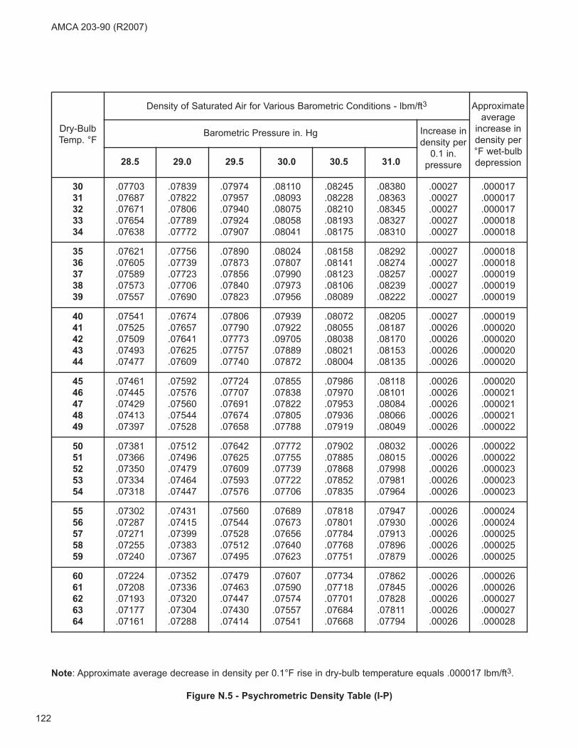
Dry-Bulb
Temp. °F
Density of Saturated Air for Various Barometric Conditions - lbm/ft3 Approximate
average
increase in
density per
°F wet-bulb
depression
Barometric Pressure in. Hg Increase in
density per
0.1 in.
pressure28.5 29.0 29.5 30.0 30.5 31.0
30
31
32
33
34
.07703
.07687
.07671
.07654
.07638
.07839
.07822
.07806
.07789
.07772
.07974
.07957
.07940
.07924
.07907
.08110
.08093
.08075
.08058
.08041
.08245
.08228
.08210
.08193
.08175
.08380
.08363
.08345
.08327
.08310
.00027
.00027
.00027
.00027
.00027
.000017
.000017
.000017
.000018
.000018
35
36
37
38
39
.07621
.07605
.07589
.07573
.07557
.07756
.07739
.07723
.07706
.07690
.07890
.07873
.07856
.07840
.07823
.08024
.07807
.07990
.07973
.07956
.08158
.08141
.08123
.08106
.08089
.08292
.08274
.08257
.08239
.08222
.00027
.00027
.00027
.00027
.00027
.000018
.000018
.000019
.000019
.000019
40
41
42
43
44
.07541
.07525
.07509
.07493
.07477
.07674
.07657
.07641
.07625
.07609
.07806
.07790
.07773
.07757
.07740
.07939
.07922
.09705
.07889
.07872
.08072
.08055
.08038
.08021
.08004
.08205
.08187
.08170
.08153
.08135
.00027
.00026
.00026
.00026
.00026
.000019
.000020
.000020
.000020
.000020
45
46
47
48
49
.07461
.07445
.07429
.07413
.07397
.07592
.07576
.07560
.07544
.07528
.07724
.07707
.07691
.07674
.07658
.07855
.07838
.07822
.07805
.07788
.07986
.07970
.07953
.07936
.07919
.08118
.08101
.08084
.08066
.08049
.00026
.00026
.00026
.00026
.00026
.000020
.000021
.000021
.000021
.000022
50
51
52
53
54
.07381
.07366
.07350
.07334
.07318
.07512
.07496
.07479
.07464
.07447
.07642
.07625
.07609
.07593
.07576
.07772
.07755
.07739
.07722
.07706
.07902
.07885
.07868
.07852
.07835
.08032
.08015
.07998
.07981
.07964
.00026
.00026
.00026
.00026
.00026
.000022
.000022
.000023
.000023
.000023
55
56
57
58
59
.07302
.07287
.07271
.07255
.07240
.07431
.07415
.07399
.07383
.07367
.07560
.07544
.07528
.07512
.07495
.07689
.07673
.07656
.07640
.07623
.07818
.07801
.07784
.07768
.07751
.07947
.07930
.07913
.07896
.07879
.00026
.00026
.00026
.00026
.00026
.000024
.000024
.000025
.000025
.000025
60
61
62
63
64
.07224
.07208
.07193
.07177
.07161
.07352
.07336
.07320
.07304
.07288
.07479
.07463
.07447
.07430
.07414
.07607
.07590
.07574
.07557
.07541
.07734
.07718
.07701
.07684
.07668
.07862
.07845
.07828
.07811
.07794
.00026
.00026
.00026
.00026
.00026
.000026
.000026
.000027
.000027
.000028
Note: Approximate average decrease in density per 0.1°F rise in dry-bulb temperature equals .000017 lbm/ft3.
Figure N.5 - Psychrometric Density Table (I-P)
AMCA 203-90 (R2007)
122
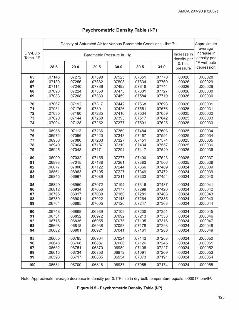
Psychrometric Density Table (I-P)
Dry-Bulb
Temp. °F
Density of Saturated Air for Various Barometric Conditions - lbm/ft3 Approximate
average
increase in
density per
°F wet-bulb
depression
Barometric Pressure in. Hg Increase in
density per
0.1 in.
pressure28.5 29.0 29.5 30.0 30.5 31.0
65
66
67
68
69
.07145
.07130
.07114
.07098
.07083
.07272
.07256
.07240
.07224
.07208
.07398
.07382
.07366
.07350
.07333
.07525
.07508
.07492
.07475
.07459
.07651
.07634
.07618
.07601
.07584
.07770
.07760
.07744
.07727
.07710
.00026
.00026
.00026
.00026
.00026
.000028
.000029
.000029
.000030
.000030
70
71
72
73
74
.07067
.07051
.07035
.07020
.07004
.07192
.07176
.07160
.07144
.07128
.07317
.07301
.07285
.07268
.07252
.07442
.07426
.07410
.07393
.07377
.07568
.07551
.07534
.07517
.07501
.07693
.07676
.07659
.07642
.07625
.00026
.00025
.00025
.00025
.00025
.000031
.000031
.000032
.000033
.000033
75
76
77
78
79
.06988
.06972
.06956
.06940
.06925
.07112
.07096
.07080
.07064
.07048
.07236
.07220
.07203
.07187
.07171
.07360
.07343
.07327
.07310
.07294
.07484
.07467
.07451
.07434
.07417
.07603
.07591
.07574
.07557
.07540
.00025
.00025
.00025
.00025
.00025
.000034
.000034
.000035
.000036
.000036
80
81
82
83
84
.06909
.06893
.06877
.06861
.06845
.07032
.07015
.07000
.06983
.06967
.07155
.07138
.07122
.07105
.07089
.07277
.07261
.07244
.07227
.07211
.07400
.07383
.07366
.07349
.07333
.07523
.07506
.07489
.07472
.07454
.00025
.00025
.00024
.00024
.00024
.000037
.000038
.000039
.000039
.000040
85
86
87
88
89
.06829
.06812
.06796
.06780
.06764
.06950
.06934
.06917
.06901
.06885
.07072
.07056
.07039
.07022
.07005
.07194
.07177
.07160
.07143
.07126
.07316
.07299
.07281
.07264
.07247
.07437
.07420
.07403
.07385
.07368
.00024
.00024
.00024
.00024
.00024
.000041
.000042
.000043
.000043
.000044
90
91
92
93
94
.06748
.06731
.06715
.06698
.06682
.06868
.06852
.06835
.06818
.06801
.06989
.06972
.06955
.06938
.06921
.07109
.07092
.07075
.07058
.07041
.07230
.07213
.07195
.07178
.07161
.07351
.07333
.07316
.07298
.07280
.00024
.00024
.00024
.00024
.00024
.000045
.000046
.000047
.000048
.000049
95
96
97
98
99
.06665
.06648
.06632
.06615
.06598
.06785
.06768
.06751
.06734
.06717
.06904
.06887
.06870
.06853
.06835
.07024
.07006
.06989
.06972
.06954
.07143
.07126
.07108
.01091
.07073
.07263
.07245
.07227
.07209
.07191
.00024
.00024
.00024
.00024
.00024
.000050
.000051
.000052
.000053
.000054
100 .06581 .06700 .06818 .06937 .07055 .07174 .00024 .000055
Note: Approximate average decrease in density per 0.1°F rise in dry-bulb temperature equals .000017 lbm/ft3.
Figure N.5 - Psychrometric Density Table (I-P)
AMCA 203-90 (R2007)
123
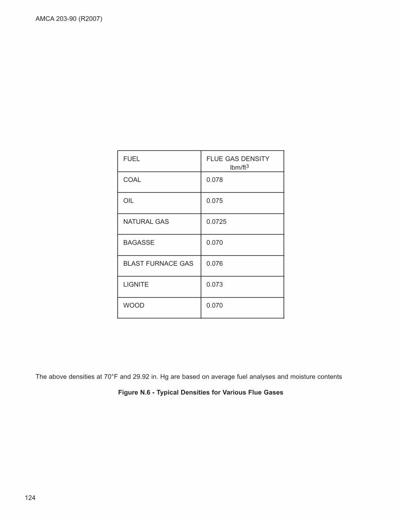
FUEL FLUE GAS DENSITY
lbm/ft3
COAL 0.078
OIL 0.075
NATURAL GAS 0.0725
BAGASSE 0.070
BLAST FURNACE GAS 0.076
LIGNITE 0.073
WOOD 0.070
The above densities at 70°F and 29.92 in. Hg are based on average fuel analyses and moisture contents
Figure N.6 - Typical Densities for Various Flue Gases
AMCA 203-90 (R2007)
124
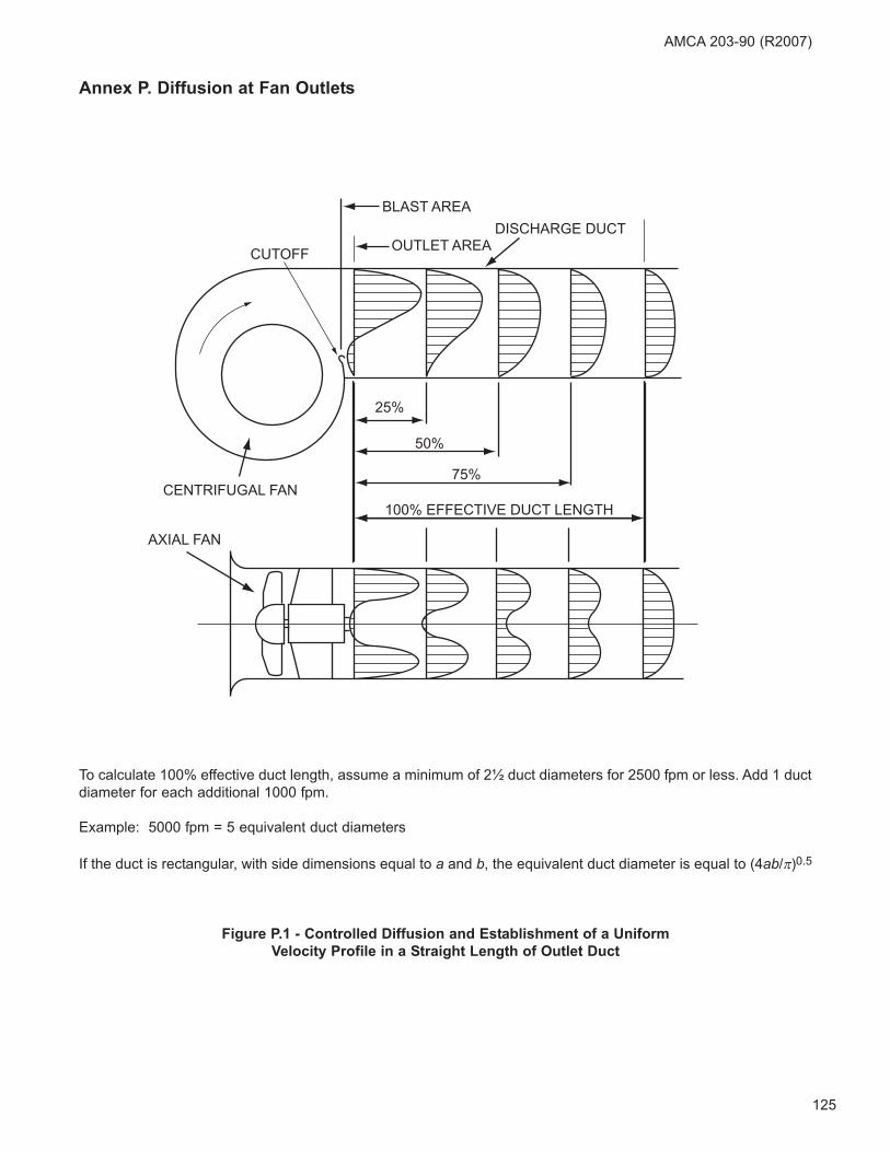
OUTLET AREA
BLAST AREA
CENTRIFUGAL FAN
AXIAL FAN
CUTOFF
DISCHARGE DUCT
25%
50%
75%
100% EFFECTIVE DUCT LENGTH
To calculate 100% effective duct length, assume a minimum of 2½ duct diameters for 2500 fpm or less. Add 1 duct
diameter for each additional 1000 fpm.
Example: 5000 fpm = 5 equivalent duct diameters
If the duct is rectangular, with side dimensions equal to a and b, the equivalent duct diameter is equal to (4ab/π)0.5
Figure P.1 - Controlled Diffusion and Establishment of a Uniform
Velocity Profile in a Straight Length of Outlet Duct
Annex P. Diffusion at Fan Outlets
AMCA 203-90 (R2007)
125
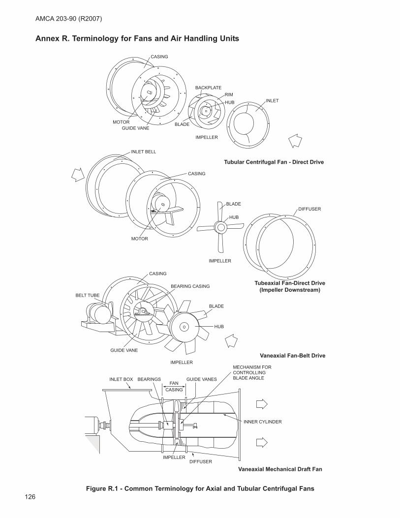
BEARINGSINLET BOX GUIDE VANES
MECHANISM FORCONTROLLINGBLADE ANGLE
INNER CYLINDER
IMPELLERDIFFUSER
BELT TUBE
CASING
BEARING CASING
BLADE
HUB
IMPELLER
GUIDE VANEVaneaxial Fan-Belt Drive
Tubeaxial Fan-Direct Drive(Impeller Downstream)
DIFFUSERBLADE
HUB
IMPELLER
INLET BELL
CASING
MOTOR
Tubular Centrifugal Fan - Direct Drive
INLET
BACKPLATERIM
HUB
IMPELLER
BLADEGUIDE VANE
MOTOR
CASING
Vaneaxial Mechanical Draft Fan
FANCASING
Figure R.1 - Common Terminology for Axial and Tubular Centrifugal Fans
Annex R. Terminology for Fans and Air Handling Units
AMCA 203-90 (R2007)
126
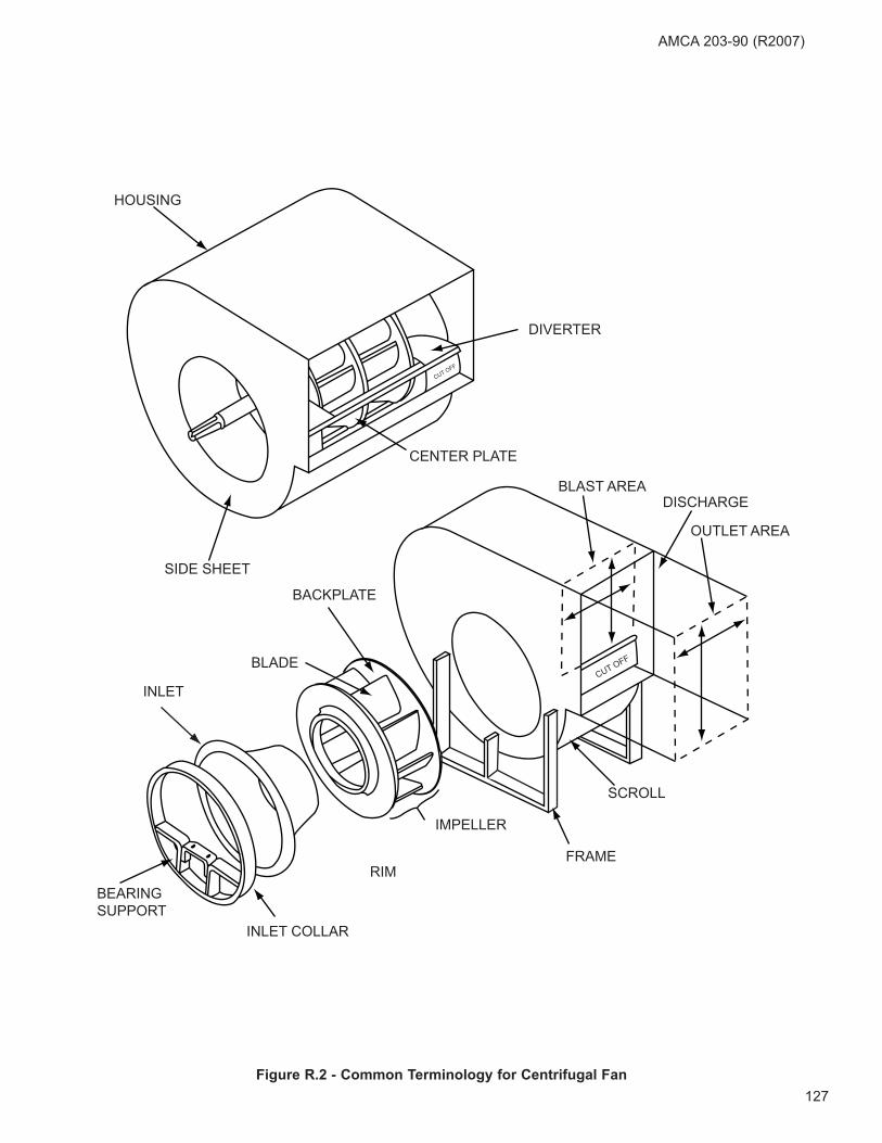
HOUSING
DIVERTER
CENTER PLATE
SIDE SHEET
CUT OFF
BEARINGSUPPORT
INLET COLLAR
INLET
BLADE
BACKPLATE
IMPELLER
RIM
CUT OFF
BLAST AREADISCHARGE
OUTLET AREA
SCROLL
FRAME
Figure R.2 - Common Terminology for Centrifugal Fan
AMCA 203-90 (R2007)
127
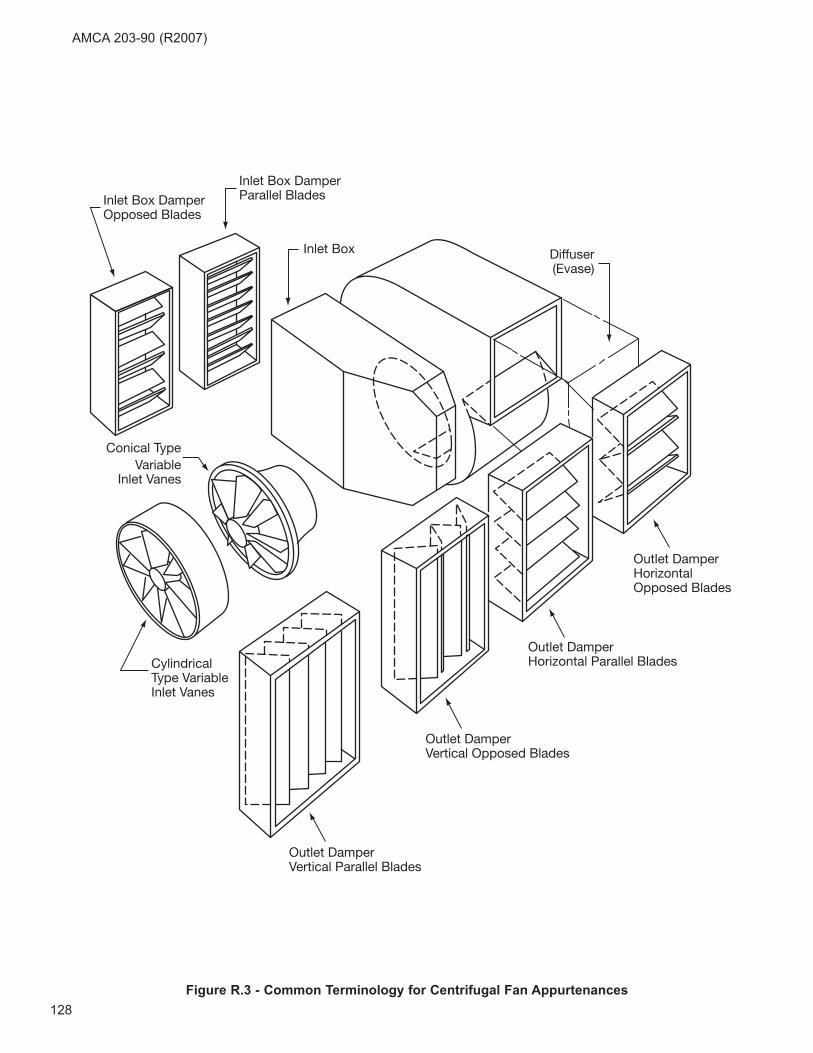
Figure R.3 - Common Terminology for Centrifugal Fan Appurtenances
AMCA 203-90 (R2007)
128
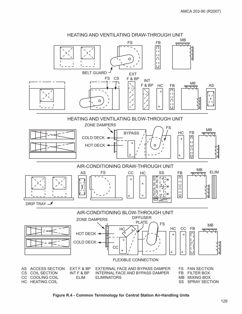
Figure R.4 - Common Terminology for Central Station Air-Handling Units
MB
MB
MB
MB
FB
FB ASHCINT
F & BP
EXTF & BPFS CS
BELT GUARD
FSMB
FBHCFS
ZONE DAMPERS
COLD DECK
HOT DECK
AS FS CC HC SS FB ELIM
DRIP TRAY
HOT DECK
COLD DECK
+
+
++
+
+
+ +
+
+++
+
+
+
++
+++
+
+
AS ACCESS SECTIONCS COIL SECTIONCC COOLING COILHC HEATING COIL
EXT F & BPINT F & BP
ELIM
EXTERNAL FACE AND BYPASS DAMPERINTERNAL FACE AND BYPASS DAMPERELIMINATORS
FS FAN SECTIONFB FILTER BOXMB MIXING BOXSS SPRAY SECTION
BYPASS
FBCCHCFS
DIFFUSERPLATE
AIR-CONDITIONING BLOW-THROUGH UNIT
AIR-CONDITIONING DRAW-THROUGH UNIT
HEATING AND VENTILATING BLOW-THROUGH UNIT
HC
ZONE DAMPERS
CC
FLEXIBLE CONNECTION
HEATING AND VENTILATING DRAW-THROUGH UNIT
AMCA 203-90 (R2007)
129
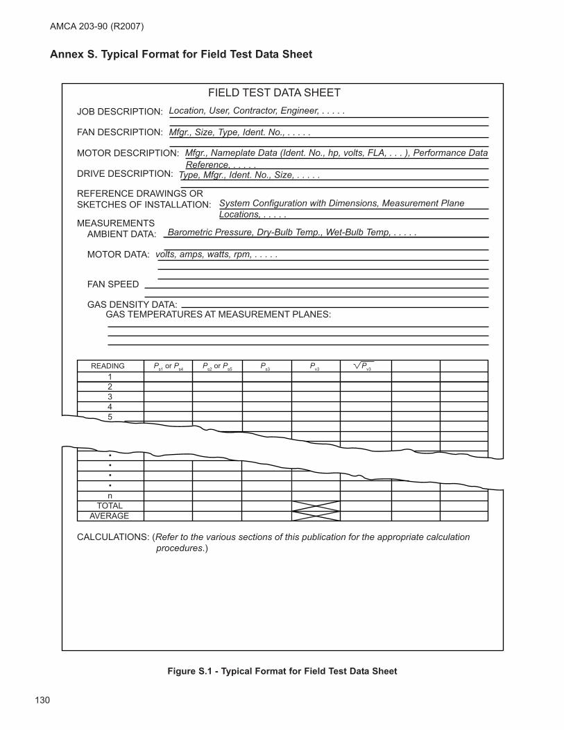
JOB DESCRIPTION:
FAN DESCRIPTION:
MOTOR DESCRIPTION:
DRIVE DESCRIPTION:
REFERENCE DRAWINGS ORSKETCHES OF INSTALLATION:
MEASUREMENTSAMBIENT DATA:
MOTOR DATA:
FAN SPEED
GAS DENSITY DATA:GAS TEMPERATURES AT MEASUREMENT PLANES:
Location, User, Contractor, Engineer, . . . . .
Mfgr., Size, Type, Ident. No., . . . . .
Mfgr., Nameplate Data (Ident. No., hp, volts, FLA, . . . ), Performance DataReference, . . . . .
Type, Mfgr., Ident. No., Size, . . . . .
System Configuration with Dimensions, Measurement PlaneLocations, . . . . .
volts, amps, watts, rpm, . . . . .
READING Ps1 or Ps4 Ps2 or Ps5 Ps3 Pv3 Pv3
21
345
TOTALAVERAGE
n
••
••
CALCULATIONS: (Refer to the various sections of this publication for the appropriate calculation procedures.)
Barometric Pressure, Dry-Bulb Temp., Wet-Bulb Temp, . . . . .
FIELD TEST DATA SHEET
Figure S.1 - Typical Format for Field Test Data Sheet
Annex S. Typical Format for Field Test Data Sheet
AMCA 203-90 (R2007)
130
AMCA 203-90 (R2007)
Annex T. Uncertainty Analysis
T.1 Introduction
In an attempt to determine the range of uncertainties
likely to be encountered in field testing of fans, a
statistical uncertainty analysis was undertaken.
Maximum and minimum uncertainties were assigned
to each quantity to be measured based on the degree
of difficulty in measuring the quantity, the previously
specified accuracies of instruments and the
conditions expected to be encountered in field
testing. These individual maximum and minimum
uncertainties were then combined statistically to
arrive at the probable range of overall uncertainties
for the fan flow rate, fan static pressure, and fan
power input. It would be unlikely, however, that any
particular field installation would have all minimum or
all maximum uncertainties occurring simultaneously.
Therefore, an agreement by the parties as to
acceptable measurement tolerances for a given
installation should be established prior to testing.
In Type A tests, it may be sufficient to accept the
results of any field test without consideration of the
probable uncertainties in the results. For Type B and
Type C tests, it may be necessary to calculate the
uncertainties. To do this, each measured quantity is
assigned an estimated uncertainty by agreement of
the parties involved and the overall uncertainty is
calculated as outlined in this annex.
T.2 General
This analysis is based on the assumption that fan
perfomance can be treated as a statistical quantity
and that the performances derived from repeated
tests would have a normal distribution. The most
probable performance would, therefore, be the mean
results based on repeated observations at each point
of operation. Only one set of observations is
specified in this publication. This analysis deals,
therefore, with the probable uncertainty in the results
obtained from a single set of observations.
The results of a fan field performance test for a single
point of operation are a combination of variables
which are normally presented graphically. Test results
will be considered to be the fan static pressure
versus flow rate and fan power input versus flow rate.
The uncertainty in results will be expressed in terms
of fan flow rate, fan static pressure, and fan power
input.
The accuracies specified in this publication are based
upon two standard deviations. This means that there
should be a 95% probability that the actual
uncertainties will be less than the specified value.
This applies only to random uncertainties. Systematic
uncertainties should be eliminated by the use of
properly calibrated test instruments. This analysis
considers only the uncertainties inherent in testing.
This publication specifies uncertainties in percent.
These are, of course, per unit uncertainties,
multiplied by 100. Absolute uncertainties which bear
the units of the quantity being measured or
calculated, are equal to the per unit uncertainty
multiplied by the measured or calculated quantity.
Since the tolerance on measured values is specified
on the basis of 95% confidence limits, the actual
deviations in results will be less than the calculated
deviations 95% of the time.
For the purposes of a field test, an uncertainty range
will be defined with minimum and maximum values.
This range of possible uncertainty is necessary to
cover the varying degrees of difficulty encountered in
performing tests in field installations. Field test
conditions range from near ideal to near impossible.
T.3 Symbols
In the analysis that follows, certain symbols and
notations are used in addition to those shown in
Annex Q.
Symbol Quantity
ex Per Unit Uncertainty in X
ΔX Absolute Uncertainty in X
R Gas Constant (ft-lb/lbm —°R)
Subscript Description
A area
b Barometric Pressure
d Dry-bulb Temperature
f Velocity Pressure
g Static Pressure
h Power Input
H Fan Power Input
N Fan Speed
P Fan Static Pressure
Q Fan Flow Rate
w Wet-bulb Depression
x Generalized Quantity (A, b, ..., ρ)
ρ Density
T.4 Measurement uncertainties
The various measurement uncertainty ranges used in
this publication are listed below. The considerations
that led to their adoption include difficulties in field
testing generally not encountered in laboratory
testing.
131
AMCA 203-90 (R2007)
T.4.1 Barometric pressure. The estimated
uncertainty in measuring barometric pressure is
between 0.3% minimum and 0.7% maximum.
eb = 0.003 (min) to 0.007 (max)
Barometric pressure is generally obtained by
portable aneroid barometer, on-site barometer
(mercury or aneroid) or by use of data obtained from
a nearby airport. The uncertainty range above is
estimated based on the use of portable or on-site
instrumentation and applicable corrections.
T.4.2 Dry-bulb temperature. The estimated
uncertainty in measuring dry-bulb temperature is
between 0.5% of absolute temperature minimum and
2.0% of absolute temperature maximum.
ed = 0.005 (min) to 0.02 (max)
The estimated uncertainty range is based on a broad
temeprature range and the likelihood of stratification.
T.4.3 Web-bulb depression. The estimated
uncertainty in measuring wet-bulb depression is
between 5°F minimum and 10°F maximum.
ew = 5/(td - tw) (min) to 10/(td - tw) (max)
The estimated uncertainty range is based on a broad
temperature range with the associated difficulties in
determining wet-bulb readings at high or low
temperatures and the likelihood of stratification.
T.4.4 Fan speed. The estimated uncertainty in
measuring fan speed is between 0.5% minimum and
1.0% maximum.
eN = 0.005 (min) to 0.01 (max)
The uncertainty range in fan speed is estimated on
the basis of portable instrumentation accuracy and
an allowance for fluctuation in fan speed.
T.4.5 Power input. The estimated uncertainty in
measuring power input is betwen 3.0% minimum and
7.0% maximum.
eh = 0.03 (min) to 0.07 (max)
The estimated uncertainty range is based on the
various measurement methods and their respective
accuracies, estimated drive losses, and the broad
horsepower range encountered in the field.
T.4.6 Pitot traverse. A properly performed field
traverse is estimated to have an accuracy of 1.5%
minimum to 7.5% maximum.
ec = 0.015 (min) to 0.075 (max)
The uncertainty range in the Pitot traverse is
estimated on the basis of traverse location, broad
range of duct sizes, nonuniform velocity profiles, and
turbulence.
T.4.7 Flow measurement area. The estimated
uncertainty in the flow measurement area is between
1.0% minimum to 2.0% maximum.
eA = 0.010 (min) to 0.020 (max)
The estimated uncertainty is based on a broad range
of duct sizes, accessibility, and the rigidity of ducts
under pressure.
T.4.8 Velocity pressure. An allowance of 2.0%
minimum to 5.0% maximum of the reading is
estimated for the mental averaging performed on a
fluctuating reading. An allowance of 1.0% minimum
to 2.0% maximum of the reading is estimated for
calibrated manometer uncertainty and relocation of
the instrument after calibration. In addition, an
allowance of 0.5% minimum to 10.0% maximum of
the reading is estimated for instrument precision. No
allowance is included for yaw on the assumption that
the Pitot-static tube is aligned within 10 degrees of
streamlines. A combined uncertainty can be written
as:
ef (min) = [(0.02)2 + (0.01)2 + (0.005)2]0.5
= 0.0229
ef (max) = [(0.05)2 + (0.02)2 + (0.10)2]0.5
= 0.1136
T.4.9 Static pressure. An allowance of 1.0%
minimum to 5.0% maximum of the reading is
estimated for the mental averaging performed on a
fluctuating reading. An allowance of 1.0% minimum
to 2.0% maximum of the reading is estimated for
calibrated manometer uncertainty and relocation of
the instrument after . In addition, a tolerance of 10%
minimum to 20.0% maximum of the fan velocity
pressure should cover the influence of Pitot-static
tube yaw or velocity influence on static pressure taps
and other possible effects. A combined uncertainty
can be written as:
eg (min) = {(0.01)2 + (0.01)2 + (0.005)2 +
[0.1 Pv/(Ps2 - Ps1)]2}0.5
= {0.000225 + [0.1 Pv/(Ps2 - Ps1)]2}0.5
eg (max) = {(0.05)2 + (0.02)2 + (0.02)2 +
[0.2 Pv/(Ps2 - Ps1)]2}0.5
= {0.0033 + [0.2 Pv/(Ps2 - Ps1)]2}0.5
132
Where the denominator in the final term in each
equation will involve Ps2 or Ps5 and Ps1 or Ps4,
whichever are measured.
The estimated uncertainty range is based on an
allowance for fluctuation in the fan-system operation,
lack of ideal measurement locations, turbulence, and
the relocation of instrumentation after calibration.
T.5 Combined uncertainties
The uncertainties in the test performance are the
result of using various values, each of which contains
a probable uncertainty. The combined uncertainty for
each of the fan performance variables is given below.
T.5.1 Density. Air density involves the various
psychrometric measurements and the approximate
formula:
Where:
V = 1.0 - 0.378 {(pe/pb) - [(td - tw)/2700]}
For random and independant uncertainties in
products, the combined uncertainty is determined as
follows:
Δρ/ρ = {(Δ70.73/70.73)2 + (Δpb/pb)2 + (ΔV/V)2 +
(ΔR/R)2 + [Δtd/(td + 460)]2}0.5
Assuming Δ70.73 and ΔR are both zero:
eρ = (eb2 + ev
2 + ed2)0.5
It can be shown that:
ev2 = [(0.00000725 tw - 0.0000542) Δ(td - tw)]2
Where:
Δ(td - tw) = Absolute uncertainty in wet-bulb depression.
Other methods for determining density are assumed
to have equal accuracy.
T.5.2 Fan flow rate. Fan flow rate directly involves
the area at the flow measuring station, the Pitot
traverse, the square root of the pressure
measurement for flow, and the square root of the
density. Uncertainties in fan speed will produce a
first-power uncertainty in flow rate when making the
fan law conversions. Combining:
eQ = [ec2 + eA
2 (ef/2)2 + (eρ/2)2 + eN2]0.5
T.5.3 Fan static pressure. Fan static pressure
directly involves static pressure measurements.
Uncertainties in density will produce a first-power
uncertainty in fan static pressure while uncertainties
in fan speed will produce a second-power uncertainty
in fan static pressure when making fan law
conversions. Combining:
ep = [eg2 + eρ
2 + (2eN)2]0.5
ρ =+( )
70 73
460
. p VR t
b
d
Table T.1
Measurement Minimum Maximum
eb 0.003 0.007
ed** 0.005 0.020
eW 5/(td - tw) 10/(td - tw)
eN 0.005 0.010
eh 0.030 0.070
ec 0.015 0.075
eA 0.010 0.020
ef 0.0229 0.1136
eg {0.000225 + [0.1 Pv/(Ps2 - Ps1)]2}0.5 {0.0033 + [0.2 Pv/(Ps2 - Ps1)]2}0.5
* These uncertainties do not account for the effect of swirl at the fan inlet. This situation must be corrected in order
to produce acceptable fan-system performance (see Section 5).
** Based on absolute temperature
AMCA 203-90 (R2007)
133
In order to simplify the application of this uncertainty
analysis to the results of field tests, the above
equation was developed on the basis of tests in
which static pressure measurements are made at a
single plane, as would be the case in which a fan is
ducted on one side only. However, the equation is
reasonably accurate for all other fan-system
configurations.
Although in most cases the determination of fan static
pressure involves Pv1, the uncertainty in determining
Pv1 is not included in the above equation on the basis
that it normally has a very small effect on the overall
uncertainty in fan static pressure.
For purposes of this publication, eP is applied directly
to Psc, which may include System Effect Factors.
T.5.4 Fan power input. Fan power input directly
involves the power measurement; in addition, when
making fan law conversions, density has a first-power
effect and speed has a third-power effect on fan
power input. Combining:
eH = [eh2 + eρ
2 + (3eN)2]0.5
T.6 Summary
The minimum and maximum measurement
uncertainties (See Table T.1) were defined earlier in
Section T.4. Summarizing, the per unit uncertainties
are as shown in Table T.1.
The uncertainty calculations lead to absolute
uncertainties in fan flow rate, fan static pressure, and
fan power input that can be applied directly to the
corresponding test results. The uncertainty results
can then be plotted as rectangles around the test
point. Intersection of the rectangles with the quoted
fan performance within the limitations of a field test.
See the examples in Section T.7.
T.7 Examples
Two examples of the calculation of uncertainties and
the method of comparison with the quoted fan curve
are included in this section. Uncertainty calculations
and comparisons have been developed for Examples
2B and 2C of Annex A. Uncertainty calculations for
Example 2B utilize all minimum uncertainty
tolerances. Uncertainty calculations for Example 2C
utilize all maximum uncertainty tolerances. It would
be unlikely that any field installation would lend itself
to all minimum or all maximum measurement
tolerances. Agreement of the parties as to acceptable
measurement tolerances for a given installation
should be established prior to testing.
AMCA 203-90 (R2007)
134
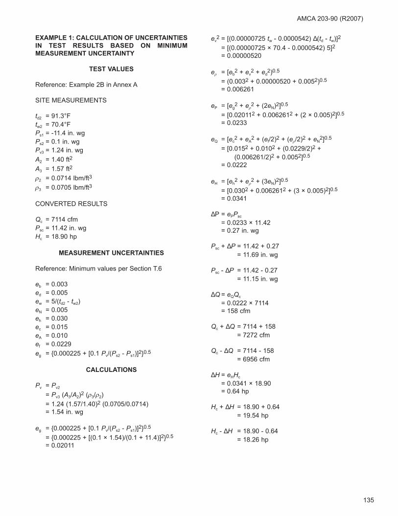
AMCA 203-90 (R2007)
EXAMPLE 1: CALCULATION OF UNCERTAINTIES
IN TEST RESULTS BASED ON MINIMUM
MEASUREMENT UNCERTAINTY
TEST VALUES
Reference: Example 2B in Annex A
SITE MEASUREMENTS
td2 = 91.3°F
tw2 = 70.4°F
Ps1 = -11.4 in. wg
Ps2 = 0.1 in. wg
Pv3 = 1.24 in. wg
A2 = 1.40 ft2
A3 = 1.57 ft2
ρ2 = 0.0714 lbm/ft3
ρ3 = 0.0705 lbm/ft3
CONVERTED RESULTS
Qc = 7114 cfm
Psc = 11.42 in. wg
Hc = 18.90 hp
MEASUREMENT UNCERTAINTIES
Reference: Minimum values per Section T.6
eb = 0.003
ed = 0.005
ew = 5/(td2 - tw2)
eN = 0.005
eh = 0.030
ec = 0.015
eA = 0.010
ef = 0.0229
eg = {0.000225 + [0.1 Pv/(Ps2 - Ps1)]2}0.5
CALCULATIONS
Pv = Pv2
= Pv3 (A3/A2)2 (ρ3/ρ2)
= 1.24 (1.57/1.40)2 (0.0705/0.0714)
= 1.54 in. wg
eg = {0.000225 + [0.1 Pv/(Ps2 - Ps1)]2}0.5
= {0.000225 + [(0.1 × 1.54)/(0.1 + 11.4)]2}0.5
= 0.02011
ev2 = [(0.00000725 tw - 0.0000542) Δ(td - tw)]2
= [(0.00000725 × 70.4 - 0.0000542) 5]2
= 0.00000520
eρ = [eb2 + ev
2 + ed2)0.5
= (0.0032 + 0.00000520 + 0.0052)0.5
= 0.006261
eP = [eg2 + eρ
2 + (2eN)2]0.5
= [0.020112 + 0.0062612 + (2 × 0.005)2]0.5
= 0.0233
eQ = [ec2 + eA
2 + (ef/2)2 + (eρ/2)2 + eN2]0.5
= [0.0152 + 0.0102 + (0.0229/2)2 +
(0.006261/2)2 + 0.0052]0.5
= 0.0222
eH = [eh2 + eρ
2 + (3eN)2]0.5
= [0.0302 + 0.0062612 + (3 × 0.005)2]0.5
= 0.0341
ΔP = ePPsc
= 0.0233 × 11.42
= 0.27 in. wg
Psc + ΔP = 11.42 + 0.27
= 11.69 in. wg
Psc - ΔP = 11.42 - 0.27
= 11.15 in. wg
ΔQ = eQQc
= 0.0222 × 7114
= 158 cfm
Qc + ΔQ = 7114 + 158
= 7272 cfm
Qc - ΔQ = 7114 - 158
= 6956 cfm
ΔH = eHHc
= 0.0341 × 18.90
= 0.64 hp
Hc + ΔH = 18.90 + 0.64
= 19.54 hp
Hc - ΔH = 18.90 - 0.64
= 18.26 hp
135
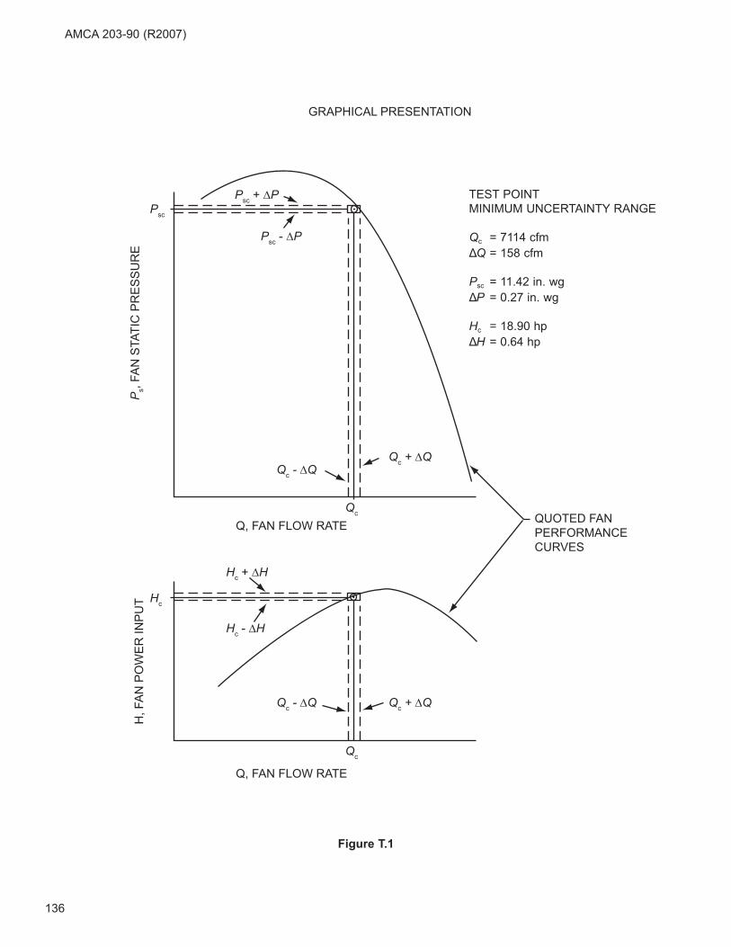
QUOTED FANPERFORMANCECURVES
Q, FAN FLOW RATE
Q, FAN FLOW RATE
Ps,
FAN
STA
TIC
PR
ES
SU
RE
H, F
AN
PO
WE
R IN
PU
T
GRAPHICAL PRESENTATION
Psc
Psc - ∆P
Psc + ∆P
Qc - ∆Q
Qc - ∆Q
Qc + ∆Q
Qc + ∆Q
Qc
Qc
Hc + ∆H
Hc - ∆H
Hc
Figure T.1
TEST POINT
MINIMUM UNCERTAINTY RANGE
Qc = 7114 cfm
ΔQ = 158 cfm
Psc = 11.42 in. wg
ΔP = 0.27 in. wg
Hc = 18.90 hp
ΔH = 0.64 hp
AMCA 203-90 (R2007)
136
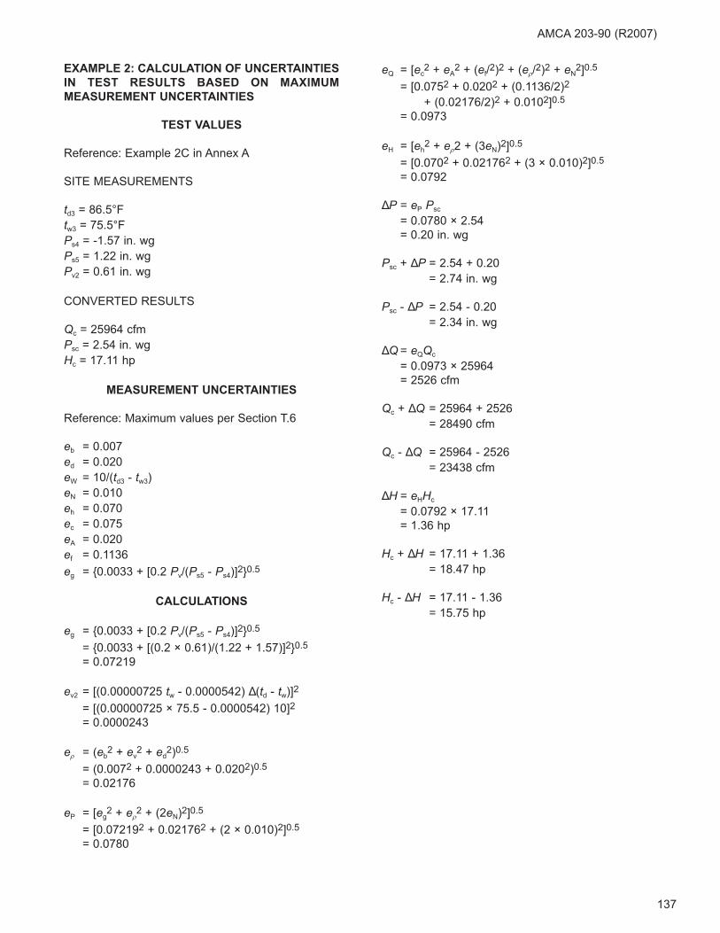
AMCA 203-90 (R2007)
EXAMPLE 2: CALCULATION OF UNCERTAINTIES
IN TEST RESULTS BASED ON MAXIMUM
MEASUREMENT UNCERTAINTIES
TEST VALUES
Reference: Example 2C in Annex A
SITE MEASUREMENTS
td3 = 86.5°F
tw3 = 75.5°F
Ps4 = -1.57 in. wg
Ps5 = 1.22 in. wg
Pv2 = 0.61 in. wg
CONVERTED RESULTS
Qc = 25964 cfm
Psc = 2.54 in. wg
Hc = 17.11 hp
MEASUREMENT UNCERTAINTIES
Reference: Maximum values per Section T.6
eb = 0.007
ed = 0.020
eW = 10/(td3 - tw3)
eN = 0.010
eh = 0.070
ec = 0.075
eA = 0.020
ef = 0.1136
eg = {0.0033 + [0.2 Pv/(Ps5 - Ps4)]2}0.5
CALCULATIONS
eg = {0.0033 + [0.2 Pv/(Ps5 - Ps4)]2}0.5
= {0.0033 + [(0.2 × 0.61)/(1.22 + 1.57)]2}0.5
= 0.07219
ev2 = [(0.00000725 tw - 0.0000542) Δ(td - tw)]2
= [(0.00000725 × 75.5 - 0.0000542) 10]2
= 0.0000243
eρ = (eb2 + ev
2 + ed2)0.5
= (0.0072 + 0.0000243 + 0.0202)0.5
= 0.02176
eP = [eg2 + eρ
2 + (2eN)2]0.5
= [0.072192 + 0.021762 + (2 × 0.010)2]0.5
= 0.0780
eQ = [ec2 + eA
2 + (ef/2)2 + (eρ/2)2 + eN2]0.5
= [0.0752 + 0.0202 + (0.1136/2)2
+ (0.02176/2)2 + 0.0102]0.5
= 0.0973
eH = [eh2 + eρ2 + (3eN)2]0.5
= [0.0702 + 0.021762 + (3 × 0.010)2]0.5
= 0.0792
ΔP = eP Psc
= 0.0780 × 2.54
= 0.20 in. wg
Psc + ΔP = 2.54 + 0.20
= 2.74 in. wg
Psc - ΔP = 2.54 - 0.20
= 2.34 in. wg
ΔQ = eQQc
= 0.0973 × 25964
= 2526 cfm
Qc + ΔQ = 25964 + 2526
= 28490 cfm
Qc - ΔQ = 25964 - 2526
= 23438 cfm
ΔH = eHHc
= 0.0792 × 17.11
= 1.36 hp
Hc + ΔH = 17.11 + 1.36
= 18.47 hp
Hc - ΔH = 17.11 - 1.36
= 15.75 hp
137
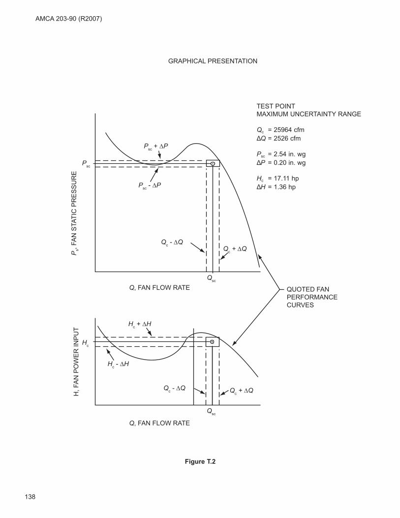
QUOTED FANPERFORMANCECURVES
Q, FAN FLOW RATE
Q, FAN FLOW RATE
Ps,
FAN
STA
TIC
PR
ES
SU
RE
H, F
AN
PO
WE
R IN
PU
T
Psc
Psc - ∆P
Psc + ∆P
Qc - ∆Q
Qc - ∆Q
Qc + ∆Q
Qc + ∆Q
Qsc
Qsc
Hc + ∆H
Hc - ∆H
Hc
GRAPHICAL PRESENTATION
Figure T.2
TEST POINT
MAXIMUM UNCERTAINTY RANGE
Qc = 25964 cfm
ΔQ = 2526 cfm
Psc = 2.54 in. wg
ΔP = 0.20 in. wg
Hc = 17.11 hp
ΔH = 1.36 hp
AMCA 203-90 (R2007)
138

AIR MOVEMENT AND CONTROLASSOCIATION INTERNATIONAL, INC.
30 West University DriveArlington Heights, IL 60004-1893 U.S.A.
E-Mail : [email protected] Web: www.amca.orgTel: (847) 394-0150 Fax: (847) 253-0088
The Air Movement and control Association International, Inc. is a not-for-profit international association of the world’s manufacturers of related air system equipment primarily, but limited to: fans, louvers, dampers, air curtains, airflow measurement stations, acoustic attenuators, and other air system components for the industrial, commercial and residential markets.