ambiguity aversion: adoption, uptake, and trends

The University of San FranciscoUSF Scholarship: a digital repository @ Gleeson Library |Geschke Center

Master's Theses Theses, Dissertations, Capstones and Projects

Spring 5-15-2017

Ambiguity Aversion: Adoption, Uptake, andTrendsAdam [email protected]

Follow this and additional works at: https://repository.usfca.edu/thes

Part of the Behavioral Economics Commons, Growth and Development Commons,International Economics Commons, and the Public Economics Commons

This Thesis is brought to you for free and open access by the Theses, Dissertations, Capstones and Projects at USF Scholarship: a digital repository @Gleeson Library | Geschke Center. It has been accepted for inclusion in Master's Theses by an authorized administrator of USF Scholarship: a digitalrepository @ Gleeson Library | Geschke Center. For more information, please contact [email protected].

Recommended CitationFranklin, Adam, "Ambiguity Aversion: Adoption, Uptake, and Trends" (2017). Master's Theses. 267.https://repository.usfca.edu/thes/267

https://repository.usfca.edu?utm_source=repository.usfca.edu%2Fthes%2F267&utm_medium=PDF&utm_campaign=PDFCoverPages

https://repository.usfca.edu?utm_source=repository.usfca.edu%2Fthes%2F267&utm_medium=PDF&utm_campaign=PDFCoverPages

https://repository.usfca.edu/thes?utm_source=repository.usfca.edu%2Fthes%2F267&utm_medium=PDF&utm_campaign=PDFCoverPages

https://repository.usfca.edu/etd?utm_source=repository.usfca.edu%2Fthes%2F267&utm_medium=PDF&utm_campaign=PDFCoverPages

https://repository.usfca.edu/thes?utm_source=repository.usfca.edu%2Fthes%2F267&utm_medium=PDF&utm_campaign=PDFCoverPages

http://network.bepress.com/hgg/discipline/341?utm_source=repository.usfca.edu%2Fthes%2F267&utm_medium=PDF&utm_campaign=PDFCoverPages




https://repository.usfca.edu/thes/267?utm_source=repository.usfca.edu%2Fthes%2F267&utm_medium=PDF&utm_campaign=PDFCoverPages

mailto:[email protected]

Ambiguity Aversion: Adoption, Uptake, and Trends

Adam J. Franklin

Department of Economics

University of San Francisco

2130 Fulton St.

San Francisco, CA 94117

Thesis Submission for the Masters of Science Degree

in International and Development Economics

e-mail: [email protected]

April 2017

Abstract: What is ambiguity aversion and what is its role as a determinant of technology

adoption? This study develops and implements a novel ambiguity preference instrument in the

context of an ongoing RCT pilot program in southwest Uganda promoting adoption of an

improved variety of sweet potato. No correlation between ambiguity aversion and crop adoption

is observed, although it is suspected that RCT treatment arms including supply- and demand-

side information reduced the ambiguity of the new variety, probably overcoming any

ambiguity-preference-related constraints and clouding the picture. Methodological lessons

learned regarding the development and implementation of an apporopriate ambiguity

preference measure point to a promising future.

I wish to thank my graduate advisor Yaniv Stopnitzky and professors Jesse Anttila-Hughes,

Alessandra Cassar, Michael Jonas, Elizabeth Katz, Man-Lui Lau, Mario Muzzi, M.C. Sunny

Wong, Bruce Wydick for their unconditional support, patience, and enthusiasm throughout

the process of preparing for and producing this paper. I wish to thank as well the entire IDEC

class of 2017 for your friendship, collaboration, and helpful comments over the last two years

and my family and friends for all of your love and kindness, without which this paper would

not have been possible.

1

1. Introduction

There exist two distinct fundamental types of uncertainty an individual may face: risk

and ambiguity. A situation involving risk is one in which the outcome distribution is known,

subjectively at least, whereas in an ambiguous situation it is not. A relevant example is that

of the rural farmer deciding how to utilize her land in the upcoming growing season. If

deciding between planting a familiar crop and renting out her land to another farmer, she

faces the choice of a known risk versus a certain, albeit lower payoff. That is, she knows how

her crops will yield in different pest, disease, and weather states of the world and she knows

the likelihood of each of these states obtaining. If, however, the choice she faces is of

planting a familiar crop versus an unfamiliar one, her choice is between a risky investment

and an ambiguous one.

While contemporary economic theory has recognized the importance of human risk

preference and incorporated it through subjective expected utility (SEU) theory (Savage,

1955), the same cannot be said of ambiguity preference. If one believes the mainstream

economic consensus that growth and technology adoption are inextricably linked, then the

omission of ambiguity preference from choice theory must be quite disconcerting.

This study introduces and implements a novel instrument to measure the ambiguity

preference of an individual. It then attempts to estimate the effect of that preference on the

decision to adopt an improved variety of sweet potato by smallholder farmers in

southwestern Uganda in the presence of an agricultural outreach program promoting the new

crop. Due to a lack of funds with which to implement an instrument with a payoff, the

measure frames its exercise as a 'game,' offering the participant the chance to 'win' a moral

victory. It follows the form of Binswanger's (1980) now ubiquitous risk measure, asking

respondents to make a series of eleven binary choices, in this case between a risk with

2

precisely known odds, varying in ten-percentage-point increments from zero to 100, and a

risk with unknown odds. Adoption of a loan offered by one of the treatment arms of the pilot

is also analyzed.

Unlike Engle Warnick (2007) and Ross (2010) I find no effect of ambiguity

preference on improved crop adoption. It is possible that existing components of the outreach

program, specifically the proliferation of supply-side information and the establishment of

model gardens to demonstrate best practices in most treatment villages, acted to reduce the

level of ambiguity faced by individual farmers and subsequently relax the constraint imposed

by any ambiguity preference they may have. It is also possible that ambiguity preference is

not a significant determinant of crop adoption in the setting and context observed.

This study does find strong hints of a positive correlation between loan adoption and

ambiguity aversion, with an increase of as much as 25 percentage points in the likelihood of

accepting a loan when offered for ambiguity averse (AA) individuals versus non-AA

individuals. This is a curious result, similar to findings by Bryan (2010) where adoption of a

financial services product correlates positively with ambiguity aversion. Possible

explanations for this abound but financial technologies are inherently unique and require

special attention that is beyond the scope of this paper.

2. Literature Review

2.1 Ambiguity and Risk

The study of decision under uncertainty dates at least as far back as Daniel Bernoulli's (1738)

original statement of the expected utility hypothesis. Two centuries passed before von

3

Neumann and Morgenstern's (1944) investigation into the axioms under which the

proposition holds and the study of this key component of decision-making behavior finally

began to advance on firmer empirical and mathematical ground. Savage (1955) extended

expected utility theory to include subjective beliefs (SEU), cementing what has become a

central pillar of the paradigm of contemporary economic theory.

Ellsberg's (1961) two-urn experiment, however, demonstrated a broadly applicable

instance in which individuals consistently exhibit a preference for risks with precisely known

oods versus risks with imprecisely known odds, what is now commonly known as ambiguity

aversion. This is a violation of SEU theory which, as it stands, fails to distinguish between

the two types of uncertainty and subsequently implies indifference between them. Ellsberg's

experiment illuminates the importance of this 'Knightian', or unknowable, uncertainty

(Knight, 1921); distinguishing ambiguity from risk and suggesting the need for a remedy to

SEU theory.

Subsequent empirical studies have built on Ellsberg's work, finding that individuals

are willing to pay to avoid imprecisely known risks in favor of precisely known (but

knowably equivalent) ones (Becker and Brownson, 1964; Chow and Sarin, 2001), that this

preference persists in experimental market settings (Sarin and Weber, 1993), and that even

experienced business owners and managers, who may reasonably be assumed to behave as

experienced and well-conditioned expectation-value-maximizers, exhibit such a preference

(Chesson & Viscusi, 2003).

While the distinction between risk and Knightian uncertainty is now well-established,

the path toward incorporating the latter into SEU theory remains unclear. Economists, to be

fair, will be hard-pressed to measure the effect of an individual's ambiguity preference on her

decision making without first measuring that preference! And so we come to the first hurdle.

4

There remains, as of yet, no consensus on a proper instrument with which to measure

AA. Recent studies measuring the effect of AA on agricultural technology adoption (Engle-

Warnick, 2007), (Bryan, 2010), (Ross, 2010) employ decision sheets with five binary

choices to be made between known and unknown risks and a penalty to be paid from the

potential reward for avoiding ambiguous risks in favor of precisely known ones. They

therefore measure the willingness to pay to avoid ambiguity when real money is at stake, a

proxy for AA, and not a particularly good one. Ambiguity takes many forms in the real world

and any relevant measure must take account of these.

A risk may have known outcomes and known payoffs for each but the frequencies of

each outcome obtaining may be completely unknown. Or, conversely, the distribution of

potential outcomes may be well-known but with the potential payoffs for each outcome

remaining unknown at decision time. More challenging yet, and nowhere to be found in any

of the discussion in the literature, is the realistic possibility of partial ambiguity, where the

odds of potential outcomes or the values of potential payoffs are imprecisely known but at

least bounded.

2.2 Agricultural Technology Adoption

The empirical study of determinants of agricultural technology adoption (ATO) has a

decades-long history dating back at least to the 1960s and studies coinciding with the arrival

of the Green Revolution in the developing world. Feder and Zilberman authored the most

widely-cited meta-analysis of empirical research in the field to date (1985) reviewing

findings regarding the effects of farm size, risk and uncertainty, human capital, labor

availability, tenure, and constraints to credit and inputs. A key recommendation is the study

of ATO as a continuous as opposed to a binary variable, one this study attempts but fails to

5

follow for lack of the requisite data. Sunding and Zilberman (2001) update the following

years of work.

Engle-Warnick (2007), Bryan (2010), and Ross (2010) are the only three studies done

to date which specifically investigate the role of AA on ATO and only Engle-Warnick (2007)

has been published. All find that ambiguity aversion itself is an important determinant of

technology adoption, although all have small sample sizes.

Missing from the literature is empirical evidence regarding the roles of age,

education, and other demographic observables in driving an individual's ambiguity

preference. The closest thing to such an analysis is Borghans, et al. (2009) paper comparing

ambiguity preferences between male and female subjects. This study aims to be the first to

address these questions.

3. Methodology

3.1 Randomized Control Trial

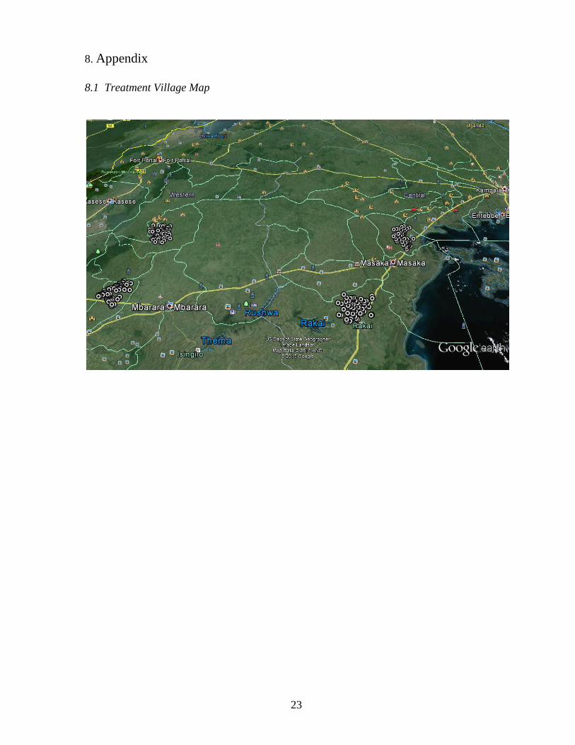
This study piggybacks on an ongoing agricultural outreach pilot program, designed

as a randomized control trial (RCT), in southwest Uganda. The Government of Uganda,

Japan Social Development Fund (JSDF) of the World Bank, and the NGO BRAC

collaborated to fund and implement the RCT. It was designed to test the effect on improved

crop adoption by smallholder farmers (<5 acres cultivated by household) of relaxing

constraints on supply- and demand-side information, credit, savings, and risk. The new crop

is a vitamin-A biofortified orange-fleshed sweet potato (OFSP), selectively bred (non-

genetically modified) over several generations to increase vitamin-A concentration. The goal

6

is to address vitamin-A deficiency (VAD), part of the broader trend of targeting

micronutrient malnutrition in the developing world with biofortified staple crops.

The World Health Organization (WHO) estimates that over half of the world's

population does not consume enough of each micronutrient to support good health. This

'hidden hunger' can have severe short- and long-term impacts ranging from lethargy and

reduced ability to fight infection, to blindness, impaired physical and cognitive development,

and death. The WHO estimates that VAD affects 250 million preschool-age children around

the world. Between 250 and 500 thousand go blind annually and half of these die within the

following year (WHO).

Previous interventions have typically used oral supplements in the form of tablets or

liquid drops to treat deficiencies of vitamin A, iron, and zinc. While effective for those who

receive treatment, supplement-based interventions frequently fail to reach those most in need

and, in any case, require indefinite funding and attention. Recently the alternative method of

staple crop biofortification has gained traction. Improved staple crops implicitly target those

most in need as the individuals who rely most heavily on staples, the poorest, are the ones

most susceptible to hidden hunger. The method has the added benefit that once the improved

variety is adopted, it remains in an area indefinitely and at zero cost (Graham, 2001). The

efficacy of OFSP in reducing VAD was demonstrated by Low’s (2007) study in rural

Mozambique.

The most significant open question that remains regarding such interventions is an

economic one: How to get people to adopt the improved crop variety? What are the

determinants of agricultural technology adoption in less developed countries?

BRAC and the Government of Uganda target southwestern Uganda as the site of the

JSDF OFSP pilot study due to the region’s significant discrepancy between income and

nutrition outcomes which fall significantly above and below national averages, respectively.

7

The RCT covers 210 villages, including 30 control villages, delivering layered treatments

over two years (four growing seasons) including relaxing constraints on supply- and demand-

side information, agricultural inputs, credit, savings, and risk. There are seven treatment arms

of 30 villages each, including control, and the treatment schedule is as follows.

Agricultural interventions include a workshop at the beginning of each growing

season for new OFSP farmers and an allotment of enough OFSP vines to plant 1/4 acre.

Support is provided by agriculture project assistants (PAs) who visit each village on a

quarterly basis. One resident is designated a Community Agriculture Promoter (CAP) in

most villages to provide regular support for her neighbors and to maintain a model garden in

which she showcases best agricultural practices.

Health interventions include monthly informational sessions conducted in each

village by health PAs covering infant, child, and maternal health and nutrition issues. These

highlight, among other concepts, the importance of micronutrient nutrition, a balanced diet,

and the role that OFSP consumption can play in this bigger picture. Growth Monitoring and

Treatment Arm Clusters Observations per cluster

Sample

T1: Agricultural Interventions Only

30 40 1200

T2: Agriculture + Health

120 40 4800

Sub-treatments of T2 T2a: T2+Credit 30 40 1200 T2b: T2+Voucher 30 40 1200 T2c: T2+Insurance 30 40 1200 T2d: T2 Only 30 40 1200 Total 120 4800

T3: Health Only 30 40 1200 Control 30 40 1200 Total Sample 210 8400

8

Promotion (GMP) is also conducted for children under two at these monthly sessions. This

involves measuring and recording the weight of each child in order to observe individual

growth trends and to enable intervention if necessary. Additionally, one resident is

designated a Community Health Promoter (CHP) in most villages to provide regular

informational support for her neighbors.

All four Tier 2 treatments include both agricultural and health interventions.

Residents of T2a villages are offered the option to take out a loan in order to grow more

OFSP (whether it be used to acquire land, labor, or other inputs). Residents of T2b villages

are offered the option to purchase a voucher for OFSP vines and fertilizer at harvest to be

redeemed at the next planting season, a savings mechanism. Residents of T2c villages are

offered a guaranteed buyback of a fixed quantity of OFSP at a fixed price prior to planting

the crop, a sort of market insurance.

Sampling was done in two phases: at the household and village level. A census was

conducted in 2013 of all households in the four districts where the study takes place.

Households were selected for participation based on the following criteria:

-Agricultural households cultivating five or fewer acres of land

-Households containing a woman of reproductive age (15-49 years)

-Households containing a pregnant woman or child less than two years of

age

-Female-headed households of a woman of reproductive age

Six treatment arms and one control group were randomly assigned at village level.

These treatments were evenly distributed across four BRAC branch offices. The

randomization was balanced on village-level variables BRAC branch, village size, market

access, and access to health clinics.

9

The random household sampling and random assignment of villages to treatments

was done in conjunction such that a highly targeted sample and a perfectly balanced

randomization was generated. To ensure this, the process of household sampling, village

assignment, and balance testing for 1000 random draws was repeated, thus selecting the draw

that both minimized the maximum t-statistic and contained the least number of significant

differences (p-value<0.1) between treatment and control groups across the balance variables

of interest (Bbosa, 2015).

treatmentTI | Age Education AA

Control: No Inte | 38.06722 6.46492 5.604816

T1: Agriculture | 37.48778 6.27814 5.601173

T2a: Agriculture | 39.76208 6.364047 6.07764

T2b: Agriculture | 38.26126 5.986251 5.603531

T2c: Agriculture | 38.49009 6.231897 5.810606

T2d: Agriculture | 38.54041 5.936842 5.682021

T3: Health Only | 38.05009 6.138418 5.718935

The table above displays respondents' age, education, and ambiguity aversion by treatment

group, showing no significant heterogeneity.

The baseline survey was conducted from April to June 2014 by a hired firm. 7,694

surveys were completed from a targeted sample of 8,400. Enumerators collected data using

paper surveys which were then digitally encoded by BRAC employees. Intervention began

before the first growing season of 2015 in January and continued through the end of 2016

over four growing seasons. The midline survey was completed from August to September

2016, after three growing seasons, with the endline survey to come in 2017-2018. 7,334

surveys were completed from the group of 7,694 households which completed the baseline

10

survey. Enumerators were hired and trained by BRAC directly and the survey was completed

using the mobile platform SurveyCTO.

3.2 Risk Preference Instrument

The baseline survey risk preference instrument utilized a series of five binary choices

between a potential coin toss for 200 thousand Uganda shillings (approximately 70 U$D at

the time) and a fixed payoff of 40, 60, 80, 100, and 140 thousand Uganda shillings, in

increasing order. For this analysis, risk averseness was defined as a binary variable, with

respondents labelled as risk-averse if they switch to the guaranteed payoff at 40, 60, 80, or

100 thousand (equivalent expectation value as coin toss) Ugandan shillings.

3.3 Ambiguity Preference Instrument

To measure ambiguity aversion, I designed a novel instrument based on Binswanger's

(1980) risk aversion instrument and included it on the midline survey, which attempted to

follow up with original respondents from baseline. Like Binswanger's, the instrument is a

schedule of binary choices to be completed in order by each individual. But whereas his

asked the respondent to choose between a guaranteed payoff and taking a known risk for a

greater possible known payoff, this measure asks respondents to choose between a known

risk for a known payoff and an unknown risk for the same known payoff.

The exercise was framed as a ‘game’ as games are culturally acceptable and familiar

to Ugandans, although they are much more commonly enjoyed by men than women (who

constitute over 90% of respondents). Enumerators were given blue and green hair curlers to

act as the ‘balls’ and to use a simple plastic bag as the ‘urn’ as props to physically

11

demonstrate the game to respondents. They were instructed to read verbatim from the

instrument (see Appendix) while explaining and playing the game for the sake of uniformity.

Respondents were first asked to choose between a risk with a zero percent chance of a

win and an unknown risk. This was demonstrated as a bag of ten hair curlers, all blue, with a

green needing to be drawn for the win. The total number of curlers was held constant at ten,

with the proportion varying from zero green to ten green, one at a time. Multiple ambiguity

aversion indices combining the experimental data were constructed and explored. These are

covered in the analysis section.

4. Model and Hypothesis

Logit and probit analyses are utilized to analyze the adoption decision of OFSP

against risk aversion as measured at baseline and ambiguity aversion as measured at midline.

Tribe dummies are included in the second round of regressions, an important determinant of

OFSP adoption as for some tribes, sweet potato is a common staple, whereas for others it is

regarded as pig food. Controls are added in the third round. They include age, age squared,

education, household size, farm size, and tribe.

Model: (OFSP Adoption)i = 0 + 1RA_bi + 2AAi + 3Treatment Groupi +

nControlsi i

Null Hypothesis: H0: 2 = 0

12

5. Analysis

5.1 Preliminary Ambiguity Preference Indices

The original idea for an amiguity preference index, AA1, was to generate a discrete

index, ranging from 0 to 11 taking whole number values. The ambiguity preference

instrument only has 12 possible rationally consistent responses (actually 10 if one argues that

it is irrational to take a risk with guaranteed zero odds versus one with an unknown chance of

success, and alternately irrational to take a risk with unknown odds versus one with

guaranteed success). An individual who always prefers the known odds, regardless of their

level, is extremely ambiguity averse and the index assigns a value of 11. On the other hand,

one who always takes the unknown odds relative to known is ambiguity-loving, and is

assigned a value of 0. The AA1 index varies linearly between these two extremes. This

would have made a decent measure had more than 25% of responses been rationally

consistent, but as it omits all others, it proved far from ideal.

The next step, AA2, was to utilize a first-switch definition of ambiguity preference,

assigning an index value for each individual based on her first switch from the unknown to

known odds, as the known odds increase. The benefit of this method is that it avoids

discarding the responses of 75% of individuals, the drawback being that it omits a high

percentage of the information contained within each individual response. This is a balancing

act that remains unavoidable unless other concessions are made. It led directly to the creation

of the AA6 and AA7 indices which succeed in not omitting large numbers of

respondents/responses, but do so at the cost of introducing the arbitrary assignment of index

values.

13

Both AA1 and AA2 also have the added drawback of assuming linearity in the nature

of ambiguity preference and its effects on decision making; that is to say that they impose the

idea that going from 3 to 6 (ambiguity loving to mildly ambiguity averse) should have the

same effect as going from 8 to 11 (moderately ambiguity averse to maximally ambiguity

averse). They additionally assume that the effect of an individual being ambuiguity loving on

her choices will be opposite of the effect of her being ambiguity averse. In this spirit, AA3

and AA4 were built on AA1 and AA2, respectively, but assigned values from 0 to 5.

Ambiguity loving and neutral individuals were assigned the value 0, while ambiguity averse

individuals were assigned a value from 1 to 5, whether by the rationally-consistent-

observation method of AA1 or the first switch method of AA2.

5.2 AA8

AA8 is constructed on the first switch method of AA2 but is binary. Ambiguity

averse individuals are assigned a value of 1, others 0. This is an additional step to try to limit

the introduction of arbitrary levels to the ambiguity indices as well as to avoid any

assumption of linearity. The coarseness of the binary measure, it was hoped, would also help

to better resolve any effect of ambiguity preference on decision making.

5.3 AA5

AA5 is constructed similarly to AA8, except that respondents are only defined as

ambiguity averse if they switch to the known risk at or before 30%. This is a binary index

indicating those who are, therefore, highly ambiguity averse or not.

14

5.4 AA6

AA6 is an incremental disrete index varying from -16 to 16, constructed by utilizing

all responses. A series of intermediate variables was defined with value 5 (for the first

variable) if the respondent selects the known zero percent risk as opposed to the one with the

unknown odds (maximally and irrationally ambiguity averse) and zero otherwise. The second

intermediate variable takes the value 4 if the respondent selects the known 10 percent risk as

opposed to the unknown one, and zero otherwise, and so on. The values that the intermediate

variables take then change to zero or negative one, zero or negative 2, and so on for

respondents who take the ambiguous risk when the known risk is 60%, 70%, etc. Responses

when the known risk is 50% are omitted.

AA6 for each individual is defined as the sum of these intermediate variable values,

so individuals with a positive AA6 can be said to be ambiguity averse, zero AA6 ambiguity

neutral, and negative AA6 ambiguity loving, with a greater absolute value indicating a

stronger preference.

This weighted sum method is an alternate way of dealing with rationally inconsistent

responses that has the benefit of not ignoring the large number of responses that the first-

switch indices necessarily omit. The drawback is that the assignment of values for given

responses, and therefore the value that the index itself takes for each individual is, again,

arbitrary.

5.5 AA7

AA7 is a binary index constructed from AA6, with respondents defined as ambiguity

averse and taking value 1 if AA6 is greater than zero, and zero otherwise.

15

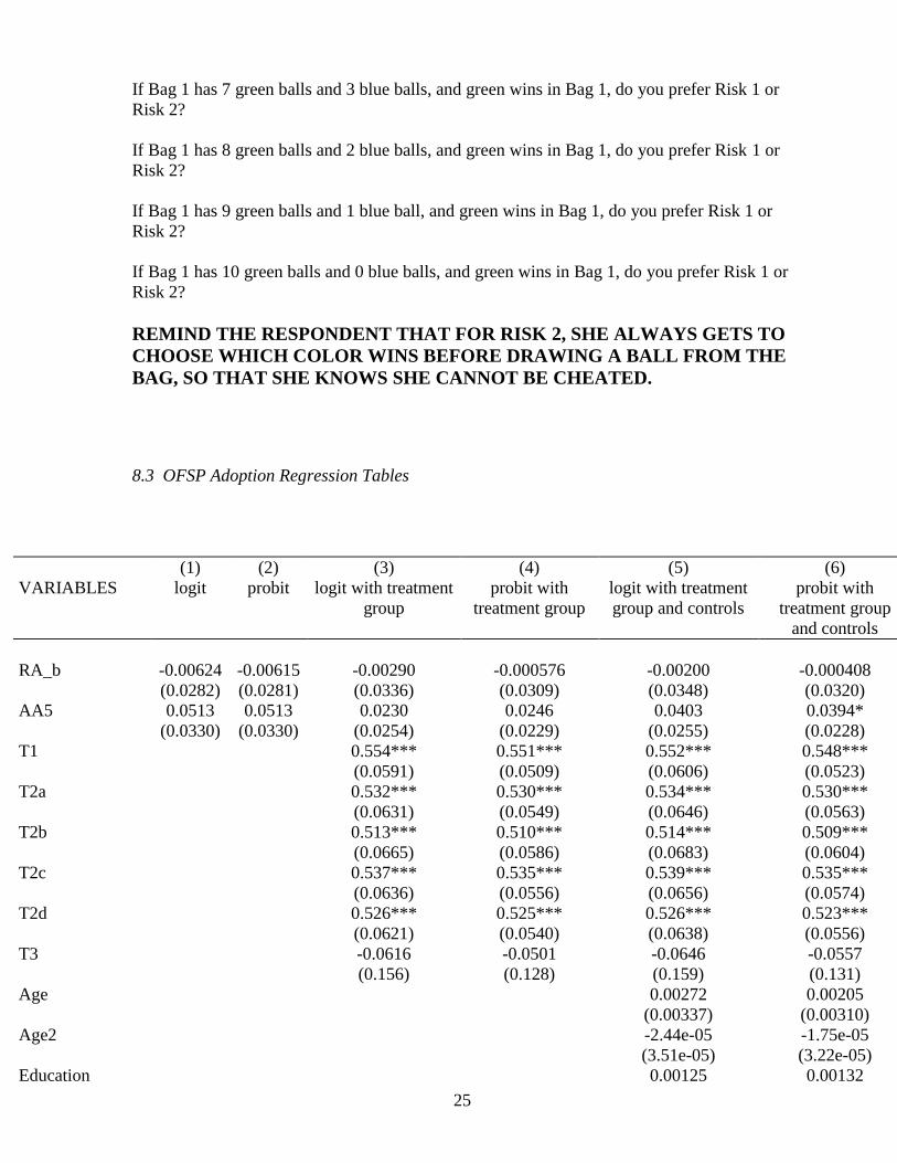
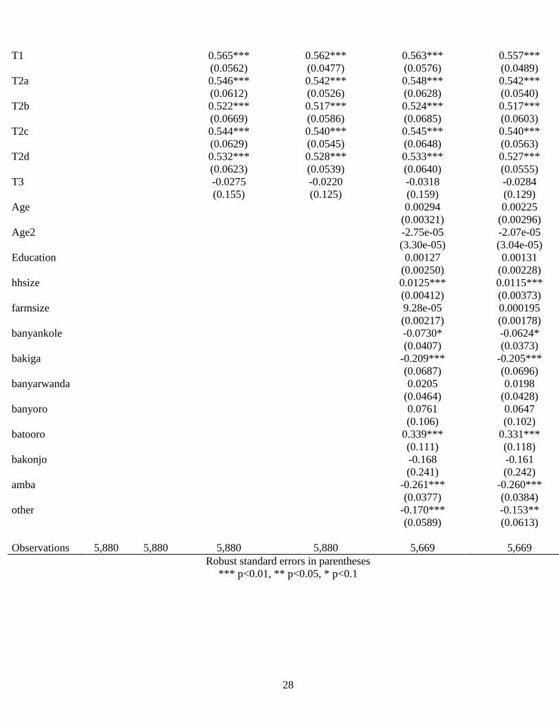
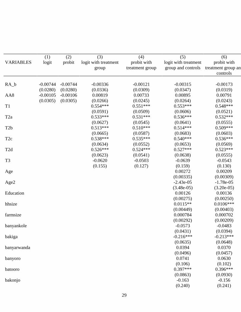
5.6 OFSP Adoption Findings

Please refer to Section 8.3 to review regression outputs for the effects of AA5-AA8

on OFSP adoption probability. Outputs listed are marginal effects at mean. Regardless of the

constructed index, findings are consistent across the board. No effect is seen on OFSP

adoption by either risk (RA_b, risk aversion at baseline) or ambiguity preference. Inclusion

of treatment group and controls does not change this and results are consistent between logit

and probit analyses. Between approximately 5,100 and 5,900 observations are included in

each regression from a total sample of 8,400 with 7,693 surveys completed at baseline and

7,033 surveys completed at midline. Attrition and data quality are obvious concerns to be

elaborated in Section 6.

We do observe strong effects of treatment group, in line with expectations. All

observations are relative to control group, and we observe that almost all treatment groups

have an OFSP adoption rate around 50-55% higher than that of control. The exception is

group T3 which only received the demand-side informational treatment and adopted OFSP at

the same rate as the control group on average. This was the one treatment group, other than

control, that did not receive the supply-side informational treatment which, importantly, also

came with OFSP starting inputs including ¼ acre worth of OFSP vines. These findings are

robust to the inclusion of controls.

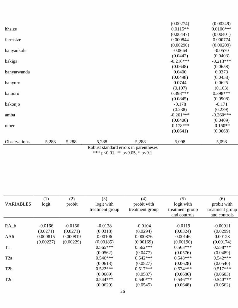
Also note that for most tribes we observe a strongly negative effect on OFSP

adoption. For context, the Baganda and Banyankole tribes each constitute roughly 49% of the

sample, and Baganda is the omitted category for the tribe variable so all observations are

relative to that group. This finding again makes a lot of sense; the Bagandas consume several

local varieties of sweet potato as a staple food, whereas other tribes in the sample regard

sweet potato as pig food. The Bagandas should be expected, therefore, to much more readily

16

adopt a new variety of sweet potato than their neighbors. Findings, again, are robust to the

inclusion of controls.

With respect to controls, only household size consistently produces a statistically

(although not economically) significant effect of about +1.25% on the probability of OFSP

adoption at 99% confidence.

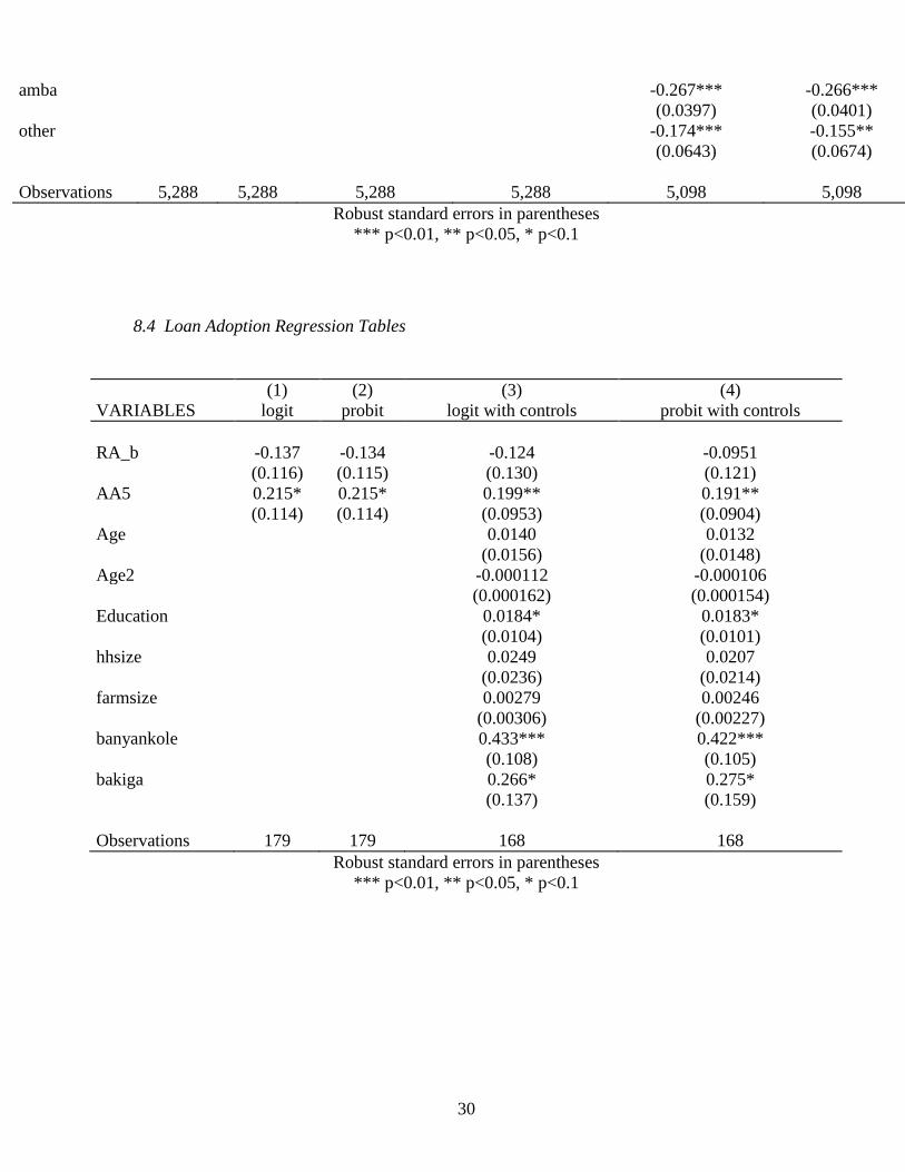
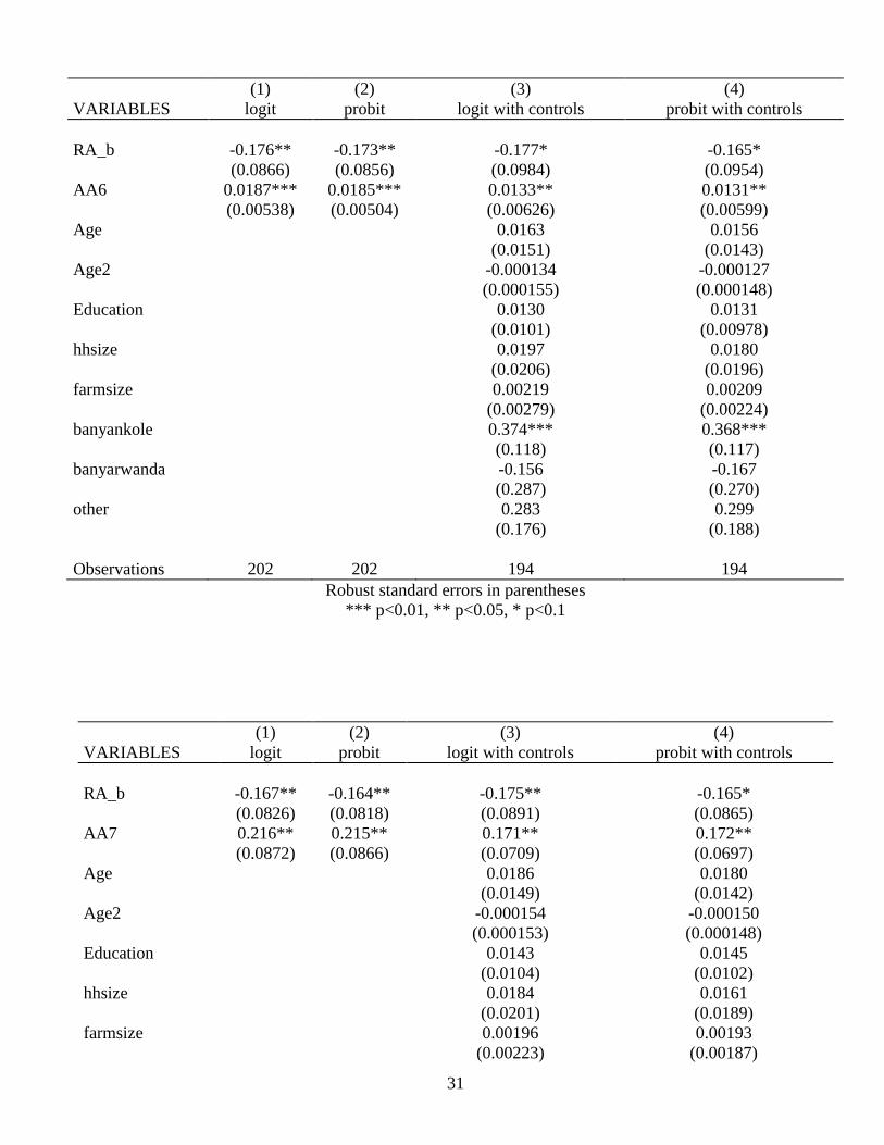
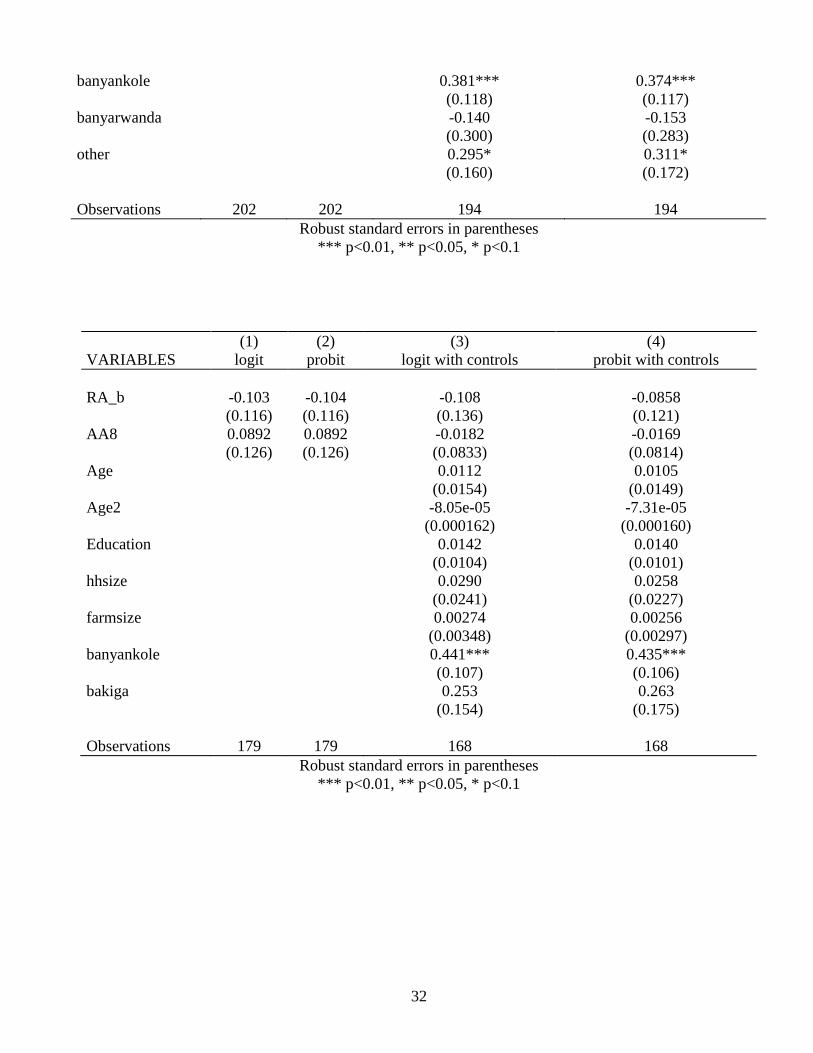
5.7 Loan Adoption Findings

The findings with respect to the effects of ambiguity preference on loan adoption for

members of treatment group T2a, the only group offered loans or ‘agricultural credit,’ are

more interesting. Ambiguity preference binary indices AA5 and AA7 (using first switch

method and weighted sum method) both indicate that the ambiguity averse are about 21.5%

more likely to accept a loan when offered than their non AA neighbors. The AA6 continuous

weighted sum index is in rough agreement as well. The output is 10 times lower, but one

must remember that AA5 and AA7 are binary and their values may be interpreted as the

effect of being ambiguity averse vs. not. AA6 varies discretely from -16 to 16 and the

resulting coefficient must be interpreted as the effect on loan adoption probability of

changing AA6 by a single unit.

All are consistent across logit and probit analyses and are robust to the inclusion of

controls. Confidence level ranges from 90% for the AA5 index to 99% for the AA6 index.

AA8, however, is not statistically different from zero, although it does have a positive point

estimate comparable and well within a standard error of the coefficients on the other indices.

Moreso than for OFSP adoption, unfortunately, sample size in the loan adoption analysis is a

concern. Only about 170-200 observations are included in this portion of the analysis from

17

1,200 households in treatment group T2a in the original sample. Results may be regarded as

intriguing but should not be thought of as definitve.

Point estimates of the effects of the binary risk aversion measure RA_b on loan

adoption fall between -10% and -18%, in line with the literature and common sense. In the

AA6 and AA7 analyses, these estimates are statistically significant to 95% confidence,

whereas in the AA5 and AA8 regressions, they are not significantly different from zero.

These results are consistent across logit and probit analyses and are robust to the inclusion of

controls. No controls were found to be significantly correlated with loan adoption.

6. Discussion

6.1 Conclusions

The primary question of this study is the effect of AA on OFSP adoption. It is the

opinion of the author that the question remains to be answered. Analysis outputs on this topic

are consistent and not statistically different from zero, although there may be a number of

reasons for this.

First and foremost, the supply- and demand-side informational treatments of the

OFSP agricultural outreach pilot program may well have acted to reduce the level of

ambiguity that the improved sweet potato variety presented to farmers. It is unfortunately

impossible to disentangle proof of this since all groups that received supply-side information

also received starting inputs including ¼ acre of OFSP vines. Future studies must reexamine

this question in the absence of such a universal informational treatment and outside of a

context in which starting inputs are provided. It is also entirely possible that ambiguity

preference does not play a role in technology adoption. Results regarding a positive

18

correltation between AA and loan adoption are suggestive and in line with findings by Bryan

(2010) but should not be considered robust.

6.2 Issues, Lessons Learned, and Looking Forward

This study was hampered by design and implementation issues. Most villages,

although receiving distinct informational treatments, are within shouting distance of one

another. In some cases, a single village was split into two, three, and in one case, as many as

four ‘different’ villages for the purpose of this study, each in a different treatment group.

Combine this proximity with the local custom of providing free vines to one’s neighbors and

it quickly becomes clear that this RCT was, by design, unable to provide distinct and separate

treatments to different villages.

Implementation issues arising from underfunding and poor incentive structures must

also be mentioned in order to inform proper interpretation of results. Project assistants, the

agriculutural and health outreach agents responsible for the day-to-day implementation of the

intervention were not paid for transport costs. Given the typical distances between BRAC

regional offices, where each began her day, and the villages to be served, it was necessary to

hire a motorcycle taxi for transport. The cost of doing this 21 or 22 days per month was

greater than the salary paid to the project assistants by about 10-30%. An improved analysis

would therefore utilize distance from village to BRAC regional office as a key control to act

as a proxy for intervention delivery intensity. It is my impression that they mostly stayed

close.

The author also remains displeased with the ambiguity preference instrument itself.

The ‘unknown’ option with which respondents are presented is constructed as such: the urn

contains 10 balls, green and blue only, with an unknown combination somewhere between 10

19

green and zero blue, and zero green and ten blue, inclusive. The respondent is allowed to

decide which color wins before drawing from the urn in order to exclude the possibility of

being tricked. This amounts to a compound lottery whose probability of success is a perfectly

knowable 50%, given the information provided and given that the respondent can do the

analysis, which leads to the next point.

The limited numeracy of most respondents was a key challenge in playing this

unavoidably mathematical game. It was often slow and difficult to explain the game, even

with physical props, and it was often unclear how well respondents ultimately understood it.

This must be carefully taken into account as ambiguity preference measures and, even

already much more mature, risk measures are developed in the future. In the context of this

study and given the compound lottery that is the risk with an ‘unknown’ chance of success,

this was surely a boon. In testing, however, even graduate students and Ph.D.s of economics

seemed not to notice and still typically selected known odds of 40% over the ‘unknown’ yet

knowable 50% lottery. The internal validity of the instrument itself, to this author, remains an

open question and one that requires more attention and debate.

Another concern is uniformity of implementation. Appendix 8.5 shows a histogram of

respondents’ AA2 first-switch index, grouped by enumerator. There is severe heterogeneity

in distribution width, center, and general form. Given this evidence and the nuanced and

subtle nature of the measure it must be argued that, going forward, much attention must be

paid to the strict uniformity of how the ‘game’ is played if results between and even within

studies are to be compared.

The challenges then are many and subtle and difficult, but if one believes that growth

and technology adoption are inherently intertwined, economics as a field must learn to

properly define, measure, and research the effects of this key human preference regarding

ambiguity. This is a relatively low-hanging fruit, and potentially a big one.

20

7. References

Adesina, A. A., & Baidu-Forson, J. (1995). Farmers' perceptions and adoption of new

agricultural technology: evidence from analysis in Burkina Faso and Guinea, West

Africa. Agricultural economics, 13(1), 1-9.

Akay, A., Martinsson, P., Medhin, H., & Trautmann, S. T. (2012). Attitudes toward

uncertainty among the poor: an experiment in rural Ethiopia. Theory and

Decision, 73(3), 453-464.

Barham, B. L., Chavas, J. P., Fitz, D., Salas, V. R., & Schechter, L. (2014). The roles of risk

and ambiguity in technology adoption. Journal of Economic Behavior &

Organization, 97, 204-218.

Bbosa, Francis Fuller. An Innovative, Integrated Approach to Enhance Smallholder Family

Nutrition, Uganda Baseline Report, BRAC Uganda Research and Evaluation Unit

(REU), April 2015.

Becker, S. W., & Brownson, F. O. (1964). What price ambiguity? Or the role of ambiguity

in decision-making. Journal of Political Economy, 72(1), 62-73.

Bernoulli, D. (1954). Exposition of a new theory on the measurement of risk. Econometrica:

Journal of the Econometric Society, 23-36.

Binswanger, H. P. (1980). Attitudes toward risk: Experimental measurement in rural

India. American journal of agricultural economics, 62(3), 395-407.

Borghans, L., Heckman, J. J., Golsteyn, B. H., & Meijers, H. (2009). Gender differences in

risk aversion and ambiguity aversion. Journal of the European Economic

Association, 7(2‐3), 649-658.Bryan, G. (2010). Ambiguity and

insurance. Unpublished manuscript.

Bryan, G. (2010). Ambiguity and insurance. Unpublished manuscript.

Chesson, H. W., & Viscusi, W. K. (2003). Commonalities in time and ambiguity aversion for

long-term risks. Theory and Decision, 54(1), 57-71.

Chew, S. H., Ebstein, R. P., & Zhong, S. (2012). Ambiguity aversion and familiarity bias:

Evidence from behavioral and gene association studies. Journal of Risk and

Uncertainty, 44(1), 1-18.

Ellsberg, D. (1961). Risk, ambiguity, and the Savage axioms. The quarterly journal of

economics, 643-669.

Engle-Warnick, J., Escobal, J., & Laszlo, S. (2007). Ambiguity aversion as a predictor of

technology choice: Experimental evidence from Peru. CIRANO-Scientific

Publications 2007s-01.

21

Feder, G., Just, R. E., & Zilberman, D. (1985). Adoption of agricultural innovations in

developing countries: A survey. Economic development and cultural change, 33(2),

255-298.

Feder, G., & Umali, D. L. (1993). The adoption of agricultural innovations: a

review. Technological forecasting and social change, 43(3), 215-239.

Einhorn, H. J., & Hogarth, R. M. (1988). Decision making under ambiguity: A note. In Risk,

Decision and Rationality (pp. 327-336). Springer Netherlands.

Giné, X., & Yang, D. (2009). Insurance, credit, and technology adoption: Field experimental

evidence from Malawi. Journal of development Economics, 89(1), 1-11.

Graham, R. D., Welch, R. M., & Bouis, H. E. (2001). Addressing micronutrient malnutrition

through enhancing the nutritional quality of staple foods: principles, perspectives and

knowledge gaps. Advances in Agronomy, 70, 77-142.

Halevy, Y. (2007). Ellsberg revisited: An experimental study. Econometrica, 75(2), 503-536.

Knight, F. H. (1921). Risk, uncertainty and profit. New York: Hart, Schaffner and Marx.

Low, J. W., Arimond, M., Osman, N., Cunguara, B., Zano, F., & Tschirley, D. (2007). A

food-based approach introducing orange-fleshed sweet potatoes increased vitamin A

intake and serum retinol concentrations in young children in rural Mozambique. The

Journal of nutrition, 137(5), 1320-1327.

Ross, N., Santos, P., & Capon, T. (2010). Risk, ambiguity and the adoption of new

technologies: Experimental evidence from a developing economy. Unpublished

Manuscript.

Sarin, R. K., & Weber, M. (1993). Effects of ambiguity in market experiments. Management

science, 39(5), 602-615.

Savage, L. J. (1972). The foundations of statistics. Courier Corporation.Trautmann, S. T.,

Vieider, F. M., & Wakker, P. P. (2008). Causes of ambiguity aversion: Known versus

unknown preferences. Journal of Risk and Uncertainty, 36(3), 225-243.

Seo, K. (2009). Ambiguity and Second‐Order Belief. Econometrica, 77(5), 1575-1605.

Sunding, D., & Zilberman, D. (2001). The agricultural innovation process: research and

technology adoption in a changing agricultural sector. Handbook of agricultural

economics, 1, 207-261.

Sutter, M., Kocher, M. G., Glätzle-Rützler, D., & Trautmann, S. T. (2013). Impatience and

uncertainty: Experimental decisions predict adolescents' field behavior. The American

Economic Review, 103(1), 510-531.

22

Tymula, A., Belmaker, L. A. R., Ruderman, L., Glimcher, P. W., & Levy, I. (2013). Like

cognitive function, decision making across the life span shows profound age-related

changes. Proceedings of the National Academy of Sciences, 110(42), 17143-17148.

Von Neumann, J., & Morgenstern, O. (2007). Theory of games and economic behavior.

Princeton university press.

World Health Organization (WHO), Micronutrient Deficiencies.

http://www.who.int/nutrition/topics/vad/en/

http://www.who.int/nutrition/topics/vad/en/

23

8. Appendix

8.1 Treatment Village Map

24

8.2 Ambiguity Preference Instrument

GAME

Now I will ask you to play a game. I will give you a choice between two risks, Risk 1 and

Risk 2.

Risk 1 is a bag containing 10 balls that are either green or blue and if you pick a green ball

you win! You can see how many of the 10 balls are green and how many are blue before you

pick.

Risk 2 is a bag which also contains 10 balls that are either green or blue, but you cannot see

how many of the balls are green or blue before you pick. They may all be green, all blue, or

some mix of both. For Risk 2, you get to pick which color is the winner before you pick a

ball, so that you cannot be cheated. If you draw a ball of your chosen winning color, you

win!

In both cases, you may examine the bags after you pick, so that you can confirm that this

information is true and so you cannot be cheated.

REMEMBER:

IN BAG 1, WE KNOW HOW MANY BALLS OF EACH COLOR THERE ARE

IN BAG 2, WE DO NOT KNOW HOW MANY BALLS OF EACH COLOR

THERE ARE

If Bag 1 has 0 green balls and 10 blue balls, and green wins in Bag 1, do you prefer Risk 1 or

Risk 2?

If Bag 1 has 1 green ball and 9 blue balls, and green wins in Bag 1, do you prefer Risk 1 or

Risk 2?


Risk 2?


Risk 2?


Risk 2?


Risk 2?


Risk 2?

25


Risk 2?


Risk 2?

If Bag 1 has 9 green balls and 1 blue ball, and green wins in Bag 1, do you prefer Risk 1 or

Risk 2?


Risk 2?

REMIND THE RESPONDENT THAT FOR RISK 2, SHE ALWAYS GETS TO

CHOOSE WHICH COLOR WINS BEFORE DRAWING A BALL FROM THE

BAG, SO THAT SHE KNOWS SHE CANNOT BE CHEATED.

8.3 OFSP Adoption Regression Tables

(1) (2) (3) (4) (5) (6)

VARIABLES logit probit logit with treatment

group

probit with

treatment group

logit with treatment

group and controls

probit with

treatment group

and controls

RA_b -0.00624 -0.00615 -0.00290 -0.000576 -0.00200 -0.000408

(0.0282) (0.0281) (0.0336) (0.0309) (0.0348) (0.0320)

AA5 0.0513 0.0513 0.0230 0.0246 0.0403 0.0394*

(0.0330) (0.0330) (0.0254) (0.0229) (0.0255) (0.0228)

T1 0.554*** 0.551*** 0.552*** 0.548***

(0.0591) (0.0509) (0.0606) (0.0523)

T2a 0.532*** 0.530*** 0.534*** 0.530***

(0.0631) (0.0549) (0.0646) (0.0563)

T2b 0.513*** 0.510*** 0.514*** 0.509***

(0.0665) (0.0586) (0.0683) (0.0604)

T2c 0.537*** 0.535*** 0.539*** 0.535***

(0.0636) (0.0556) (0.0656) (0.0574)

T2d 0.526*** 0.525*** 0.526*** 0.523***

(0.0621) (0.0540) (0.0638) (0.0556)

T3 -0.0616 -0.0501 -0.0646 -0.0557

(0.156) (0.128) (0.159) (0.131)

Age 0.00272 0.00205

(0.00337) (0.00310)

Age2 -2.44e-05 -1.75e-05

(3.51e-05) (3.22e-05)

Education 0.00125 0.00132

26

(0.00274) (0.00249)

hhsize 0.0115** 0.0106***

(0.00447) (0.00401)

farmsize 0.000844 0.000774

(0.00290) (0.00209)

banyankole -0.0664 -0.0570

(0.0442) (0.0403)

bakiga -0.216*** -0.213***

(0.0648) (0.0658)

banyarwanda 0.0400 0.0373

(0.0498) (0.0458)

banyoro 0.0744 0.0625

(0.107) (0.103)

batooro 0.398*** 0.398***

(0.0845) (0.0908)

bakonjo -0.178 -0.171

(0.238) (0.239)

amba -0.261*** -0.260***

(0.0406) (0.0409)

other -0.178*** -0.160**

(0.0641) (0.0668)

Observations 5,288 5,288 5,288 5,288 5,098 5,098

Robust standard errors in parentheses

*** p<0.01, ** p<0.05, * p<0.1

(1) (2) (3) (4) (5) (6)

VARIABLES logit probit logit with

treatment group

probit with

treatment group

logit with

treatment group

and controls

probit with

treatment group

and controls

RA_b -0.0166 -0.0166 -0.0138 -0.0104 -0.0119 -0.00911

(0.0271) (0.0271) (0.0318) (0.0294) (0.0324) (0.0299)

AA6 0.000815 0.000819 0.00106 0.000876 0.00146 0.00123

(0.00227) (0.00229) (0.00185) (0.00169) (0.00190) (0.00174)

T1 0.565*** 0.562*** 0.563*** 0.558***

(0.0562) (0.0477) (0.0576) (0.0489)

T2a 0.546*** 0.542*** 0.548*** 0.542***

(0.0613) (0.0527) (0.0628) (0.0540)

T2b 0.522*** 0.517*** 0.524*** 0.517***

(0.0669) (0.0587) (0.0686) (0.0603)

T2c 0.544*** 0.540*** 0.546*** 0.540***

(0.0629) (0.0545) (0.0648) (0.0562)

27

T2d 0.532*** 0.528*** 0.533*** 0.527***

(0.0624) (0.0539) (0.0641) (0.0555)

T3 -0.0276 -0.0220 -0.0317 -0.0286

(0.155) (0.125) (0.159) (0.129)

Age 0.00291 0.00223

(0.00320) (0.00295)

Age2 -2.72e-05 -2.05e-05

(3.29e-05) (3.04e-05)

Education 0.00125 0.00130

(0.00251) (0.00229)

hhsize 0.0124*** 0.0114***

(0.00412) (0.00373)

farmsize 7.51e-05 0.000184

(0.00217) (0.00178)

banyankole -0.0732* -0.0626*

(0.0405) (0.0372)

bakiga -0.208*** -0.204***

(0.0686) (0.0695)


(0.0463) (0.0427)

banyoro 0.0743 0.0630

(0.106) (0.102)

batooro 0.339*** 0.331***

(0.113) (0.119)

bakonjo -0.162 -0.156

(0.244) (0.243)

amba -0.260*** -0.259***

(0.0379) (0.0386)

other -0.169*** -0.152**

(0.0588) (0.0612)

Observations 5,880 5,880 5,880 5,880 5,669 5,669


*** p<0.01, ** p<0.05, * p<0.1

(1) (2) (3) (4) (5) (6)


group

probit with

treatment group


group and controls

probit with

treatment group and

controls

RA_b -0.0160 -0.0160 -0.0131 -0.00992 -0.0109 -0.00831

(0.0271) (0.0271) (0.0317) (0.0293) (0.0323) (0.0297)

AA7 0.0177 0.0177 0.00695 0.00652 0.0182 0.0159

(0.0286) (0.0286) (0.0255) (0.0232) (0.0259) (0.0234)

28

T1 0.565*** 0.562*** 0.563*** 0.557***

(0.0562) (0.0477) (0.0576) (0.0489)

T2a 0.546*** 0.542*** 0.548*** 0.542***

(0.0612) (0.0526) (0.0628) (0.0540)

T2b 0.522*** 0.517*** 0.524*** 0.517***

(0.0669) (0.0586) (0.0685) (0.0603)

T2c 0.544*** 0.540*** 0.545*** 0.540***

(0.0629) (0.0545) (0.0648) (0.0563)

T2d 0.532*** 0.528*** 0.533*** 0.527***

(0.0623) (0.0539) (0.0640) (0.0555)

T3 -0.0275 -0.0220 -0.0318 -0.0284

(0.155) (0.125) (0.159) (0.129)

Age 0.00294 0.00225

(0.00321) (0.00296)

Age2 -2.75e-05 -2.07e-05

(3.30e-05) (3.04e-05)

Education 0.00127 0.00131

(0.00250) (0.00228)

hhsize 0.0125*** 0.0115***

(0.00412) (0.00373)

farmsize 9.28e-05 0.000195

(0.00217) (0.00178)

banyankole -0.0730* -0.0624*

(0.0407) (0.0373)

bakiga -0.209*** -0.205***

(0.0687) (0.0696)


(0.0464) (0.0428)

banyoro 0.0761 0.0647

(0.106) (0.102)

batooro 0.339*** 0.331***

(0.111) (0.118)

bakonjo -0.168 -0.161

(0.241) (0.242)

amba -0.261*** -0.260***

(0.0377) (0.0384)

other -0.170*** -0.153**

(0.0589) (0.0613)

Observations 5,880 5,880 5,880 5,880 5,669 5,669


*** p<0.01, ** p<0.05, * p<0.1

29

(1) (2) (3) (4) (5) (6)


group

probit with

treatment group


group and controls

probit with

treatment group and

controls

RA_b -0.00744 -0.00744 -0.00336 -0.00121 -0.00315 -0.00173

(0.0280) (0.0280) (0.0336) (0.0309) (0.0347) (0.0319)

AA8 -0.00105 -0.00106 0.00819 0.00733 0.00895 0.00791

(0.0305) (0.0305) (0.0266) (0.0245) (0.0264) (0.0243)

T1 0.554*** 0.551*** 0.553*** 0.548***

(0.0591) (0.0509) (0.0606) (0.0521)

T2a 0.533*** 0.531*** 0.536*** 0.532***

(0.0627) (0.0545) (0.0641) (0.0555)

T2b 0.513*** 0.510*** 0.514*** 0.509***

(0.0665) (0.0587) (0.0683) (0.0603)

T2c 0.538*** 0.535*** 0.540*** 0.536***

(0.0634) (0.0552) (0.0653) (0.0569)

T2d 0.526*** 0.524*** 0.527*** 0.523***

(0.0623) (0.0541) (0.0638) (0.0555)

T3 -0.0620 -0.0503 -0.0639 -0.0543

(0.155) (0.127) (0.159) (0.130)

Age 0.00272 0.00209

(0.00335) (0.00309)

Age2 -2.43e-05 -1.78e-05

(3.48e-05) (3.20e-05)

Education 0.00126 0.00136

(0.00275) (0.00250)

hhsize 0.0115** 0.0106***

(0.00449) (0.00403)

farmsize 0.000784 0.000702

(0.00292) (0.00209)

banyankole -0.0573 -0.0483

(0.0431) (0.0394)

bakiga -0.216*** -0.213***

(0.0635) (0.0648)


(0.0496) (0.0457)

banyoro 0.0741 0.0630

(0.106) (0.102)

batooro 0.397*** 0.396***

(0.0863) (0.0930)

bakonjo -0.163 -0.156

(0.240) (0.241)

30

amba -0.267*** -0.266***

(0.0397) (0.0401)

other -0.174*** -0.155**

(0.0643) (0.0674)

Observations 5,288 5,288 5,288 5,288 5,098 5,098


*** p<0.01, ** p<0.05, * p<0.1

8.4 Loan Adoption Regression Tables

(1) (2) (3) (4)

VARIABLES logit probit logit with controls probit with controls

RA_b -0.137 -0.134 -0.124 -0.0951

(0.116) (0.115) (0.130) (0.121)

AA5 0.215* 0.215* 0.199** 0.191**

(0.114) (0.114) (0.0953) (0.0904)

Age 0.0140 0.0132

(0.0156) (0.0148)

Age2 -0.000112 -0.000106

(0.000162) (0.000154)

Education 0.0184* 0.0183*

(0.0104) (0.0101)

hhsize 0.0249 0.0207

(0.0236) (0.0214)

farmsize 0.00279 0.00246

(0.00306) (0.00227)

banyankole 0.433*** 0.422***

(0.108) (0.105)

bakiga 0.266* 0.275*

(0.137) (0.159)

Observations 179 179 168 168


*** p<0.01, ** p<0.05, * p<0.1

31

(1) (2) (3) (4)


RA_b -0.176** -0.173** -0.177* -0.165*

(0.0866) (0.0856) (0.0984) (0.0954)

AA6 0.0187*** 0.0185*** 0.0133** 0.0131**

(0.00538) (0.00504) (0.00626) (0.00599)

Age 0.0163 0.0156

(0.0151) (0.0143)

Age2 -0.000134 -0.000127

(0.000155) (0.000148)

Education 0.0130 0.0131

(0.0101) (0.00978)

hhsize 0.0197 0.0180

(0.0206) (0.0196)

farmsize 0.00219 0.00209

(0.00279) (0.00224)

banyankole 0.374*** 0.368***

(0.118) (0.117)

banyarwanda -0.156 -0.167

(0.287) (0.270)

other 0.283 0.299

(0.176) (0.188)



*** p<0.01, ** p<0.05, * p<0.1

(1) (2) (3) (4)


RA_b -0.167** -0.164** -0.175** -0.165*

(0.0826) (0.0818) (0.0891) (0.0865)

AA7 0.216** 0.215** 0.171** 0.172**

(0.0872) (0.0866) (0.0709) (0.0697)

Age 0.0186 0.0180

(0.0149) (0.0142)

Age2 -0.000154 -0.000150

(0.000153) (0.000148)

Education 0.0143 0.0145

(0.0104) (0.0102)

hhsize 0.0184 0.0161

(0.0201) (0.0189)

farmsize 0.00196 0.00193

(0.00223) (0.00187)

32

banyankole 0.381*** 0.374***

(0.118) (0.117)

banyarwanda -0.140 -0.153

(0.300) (0.283)

other 0.295* 0.311*

(0.160) (0.172)



*** p<0.01, ** p<0.05, * p<0.1

(1) (2) (3) (4)


RA_b -0.103 -0.104 -0.108 -0.0858

(0.116) (0.116) (0.136) (0.121)

AA8 0.0892 0.0892 -0.0182 -0.0169

(0.126) (0.126) (0.0833) (0.0814)

Age 0.0112 0.0105

(0.0154) (0.0149)

Age2 -8.05e-05 -7.31e-05

(0.000162) (0.000160)

Education 0.0142 0.0140

(0.0104) (0.0101)

hhsize 0.0290 0.0258

(0.0241) (0.0227)

farmsize 0.00274 0.00256

(0.00348) (0.00297)

banyankole 0.441*** 0.435***

(0.107) (0.106)

bakiga 0.253 0.263

(0.154) (0.175)



*** p<0.01, ** p<0.05, * p<0.1

33

8.5 AA2 Index Histogram, by Enumerator (9 of 10 shown)

ambiguity aversion: adoption, uptake, and trends

Documents