amadou fofana a thesis for the degree of master...
TRANSCRIPT

GENOTYPE x ENVIRONMENT INTE:RACTIO:NS AND STABILITY OF GRAIN
YIELD AND SOME OTHER C:HARACT:ERS IN PEARL MILLET
[Pennisetum americanum (L.) Leekel-
by
Amadou Fofana
A THESIS
Presented to the Faculty of
The Graduate College in the University of Nebraska
In Partial Fulfillment (of Requirements
For the Degree of Master of Science
Major:: Agronomy
Under the Supervision of Professor Charles A. Francis
Lincoln, Nebraska
September, 1984

ACKNOWLEDGMEMTS
1 wish to express my sincere gratitude to my advisor, Dr. Charles
C. Francis, for his assistance.
Many thanks to Professors W.M. ROC;S, W.G. Stegmeier, and J.W.
Mararrville.
Many thanks to Leopoldo Alvarado, Dr. Mohamed Saeed, and Dr. R.F.
Mumm for their help in analyzing the data.
1 am thankful to fellow graduate students and technicians for
their help in the work that was done during this study.
1 wish also to express my gratitude to AID (Agency for Inter-
national Development) and the government of Senegal for their financial
suppo.rt and the University of Nebraska for the use of the facilities and
personnel during the study.
For their help and patience, 1 would like to thank my parents.
Amadou Fofana
ii
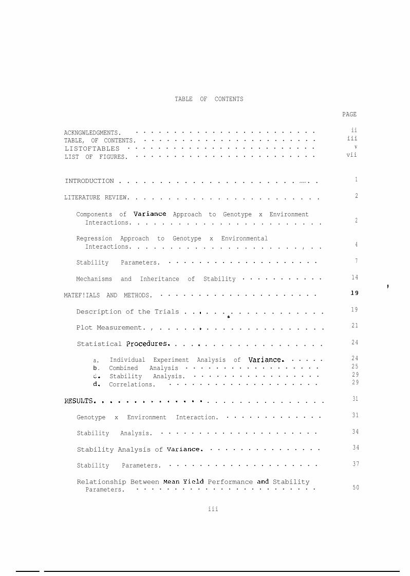
TABLE OF CONTENTS
PAGE
ACKNGWLEDGMENTS. . . . . . . . . . . . . . . . . . . . . . . . . iiTABLE, OF CONTENTS. . . . . . . . . . . . . . . . . . . . . . . . iiiLISTOFTABLES . . . . . . . . . . . . . . . . . . . . . . . . . V
LIST OF FIGURES. . . . . . . . . . . . . . . . . . . . . . . . . vii
INTRODUCTION . . . . . . . . . . . . . . . . . . . . . . ????. . 1
LITERATURE REVIEW. . . . . . . . . . . . . . . . . . . . . . . . 2
Components of Variante Approach to Genotype x EnvironmentInteractions. . . . . . . . . . . . . . . . . . . . . . . . 2
Regression Approach to Genotype x EnvironmentalInteractions. . . . . . . . . . . . . . . . . . . . . , . . 4
Stability Parameters. . . . . . . . . . . . . . . . . . . . . 7
Mechanisms and Inheritance of Stability . . . . . . . . . . . 14l
MATEF!IALS AND METHODS. . . . . . . . . . . . . . . . . . . . . . 19
Description of the Trials . . 1) . . . . . . . . . . . . . . .*.19
Plot Measurement. , . . . . . m . . . . . . . . . . . . . . .
Statistical Procedures. . . . + . . . . . . . . . . . . . . .
21
24
a. Individual Experiment Analysis of Variante. . . . . . 24b. Combined Analysis . . . . . . . . . . . . . . . . . . 25c! Stability Analysis. . . . . . . . . . . . . . . . . . 29Ci: Correlations. . . . . . . . . . . . . . . . . . . . . 29
RESULTS.............~ . . . . . . . . . . . . . . . 31
Genotype x Environment Interaction. . . . . . . . . . . . . .
Stability Analysis. . . . . . . . . . . . . . . . . . . . . .
Stability Analysis of Variante. . . . . . . . . . . . . . . .
Stability Parameters. . . . . . . . . . . . . . . . . . . . .
Relationship Between Mean Yield Performance and StabilityParameters. . . . . . . . . . . . . . . . . . . . . . . . .
31
34
34
37
50
iii

TABLE OF CONTENTS (continued)
PAGE
RESULTS (continued)
Relationship Between Stability Parameters and Coefficient(of Determination (R2). . . . . . . . . . . . . . . . . . .
Relationship Between Stability for Yield and Stability forYield Components . . . . . . . , . . . . . . I . . . . . .
DISCUSSION. . . . . . . . . . . . . . . . . . . . . . . . . . .
Genotype x Environment Interaction . . . . . . . . . - . . .
Grain Yield and Components Stability . . . . . . . . . . . .
SUMMARY <t . . . . . . . . . . . . . . . . . . . . . . . . . . .
LITERATURE CITED. . . . . . . . . . . . . . . . . . . . . . . .
50
50
53
53
54
57
59
iv
LIST OF TABLES
TABLE PAGE
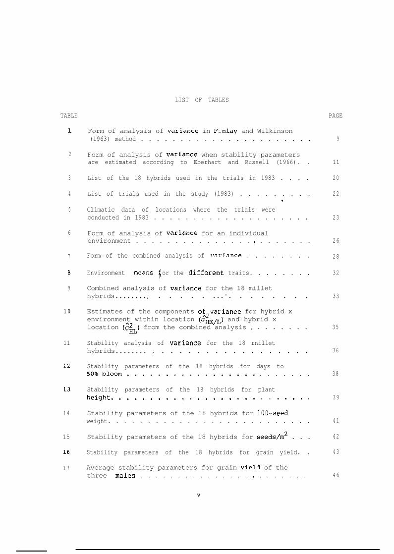
1 Form of analysis of variante in Finlay and Wilkinson(1963) method . . . . . . . . . . . . . . . . . . . . . . 9
2 Form of analysis of variante when stability parametersare estimated according to Eberhart and Russell (1966). . 11
3 List of the 18 hybrids used in the trials in 1983 . . . . 20
4 List of trials used in the study (1983) . . . . . . . . . 22*
5 Climatic data of locations where the trials wereconducted in 1983 . . . . . . . . . . . . . . . . . . . . 23
6 Form of analysis of variante for an individualenvironment . . . . . . . . . . . . . . . ,. . . . . . . . 26
7 Form of the combined analysis of variante . . . . . . . . 28
8 Environment means f or the different traits. . . . . . . . 32
9 Combined analysis of variante for the 18 millethybrids........, . . . . . ...'. . . . . . . . 33
1 0 Estimates of the components of2variance for hybrid xenvironment within location (OR,& and hybrid xlocation (âiL) from the combined analysis ., . . . . . . . 35
11 Stability analysis of variante for the 18 rnillethybrids........ , . . . . . . . . . . . . . . . . . 36
12 Stability parameters of the 18 hybrids for days to50%bloom.......,......... . . . . . . . 38
.L3 Stability parameters of the 18 hybrids for plantheight...................~ . . ..." . 39
14 Stability parameters of the 18 hybrids for lOO-seedweight. . . . . . . . . . . . . . . . . . . . . . . . . . 41
15 Stability parameters of the 18 hybrids for seeds/m2 . . . 42
16 Stability parameters of the 18 hybrids for grain yield. . 43
17 Average stability parameters for grain yiel.d of thethree males . . . . . . . . . . . . . . . o . . . . . . . 46
V

LIST OF TABLES (continued)
TABLE PAGE
18 Average stability parameters for grain yield for thes i x f e m a l e s . . . . . . . . . . . . . . . . . . . . . . . 48
19 Correlation coefficients between yield and the othertraits for means and stability parameters . . . . . . e . 52
t
vi

LIST OF FIGUFtES
FIGURE PAGE
1 Regression of yield on environmental indices for threestable hybrids. . . . . , . . . . . . . . e . . . . . . . 45
2 Regression of yiel.d on environmental indices for thethree males . . . . . . . . . . . . . . . m . . . . . . . 46
3 Regression of yield on environmental indices for threefemales......... ......O . . . . . . . . . 49
vii

INTRODUCTION
Genotype x environment interaction is of major importance in
developing improved genotypes in plant breeding. The existence of large
genot:ype x environment interaction poses a major problem of relating
phenotype performance to genetiç performance. It makes difficult the
selection of superior genotypes and inhibits progress from selection.
Therefore, it is important to understand the nature of genotype x
environment interaction to make testing and selection of genotypes more
efficient.
The relative performance of genotypes often varies from one
environment to another, i.e., there exists genotype x environment inter-
action. Testing on a large scale covering a wide range of environmental
conditions is needed to identify genotypes that interact less with the
environments or possess greatest stability.
This study was conducted to evaluate the stability and adaptation
of millet hybrids across environments in Nebraska and Kansas. The
specific objectives of this study were as follows:
- to determine the nature of genotype x environment interaction
for grain yield, days to 50% bloom, plant height, 100-seed weight, and
seeds/m2;
- to determine the stability of the hybrids for the different
traits and identify the adapted hybrids.

LITERATURE REVIEW
It is commonly observed that the relative performance of differ-
ent genotypes varies in different environments, that is, there exists
genotype x environment interaction. The presence of genotype x environ-
ment interaction contributes to the unreliability 'of trop yield over a
wide range of environments. It is in general agreement among plant
breeders that interaction between genotype and environment has an impor-
tant influence on the breeding for better genotypes. The occurrence of
large genotype x environment interaction makes the selection of superior
genotypes difficult and inhibits progress from selection. It prevents
the full understanding of genetic control of variability. Methods such
as stratification of environments have been proposed to reduce the mag- I
nitude of genotype x environment interaction, but this was of little
help in overcoming season-to-season climatic variations.
The study of genotype x environment interaction has been approached
in different ways such as the estimation of components of variante,
regression, and estimation of stability parameters. A review of these
methods is presented in this section. A discussion on the mechanisms
and inheritance of stability is also included.
Components of Variante Approach to Genotype x Environment Interactions
The earliest work providing evidenc:e of genotype x environment
interaction was reported by Fisher and Mac:kenzie (1923) in studies of
responses of different potato (Solarium tuberosum L.) varieties to
manure. This report did not involve the analysis of variante which was
introduced later. Sprague and Federer (1951) used the analysis of

:3
variante technique and showed how variante components could be used to
separate the effects of genotypes, environments and genotype x environ-
ment interaction. This was done b:y equating the observed mean squares
to their expectations and solving the resulting sets of simultaneous
equations.
The knowledge of the components of variante cari be used to iden-
tify istable genotypes. Sprague and Federer (1951) indicated that the
interaction variante component for single-cross cor-n (Zea mays L.)
hybrids repeated over locations or years was great:er than that for
double-cross hybrids. This suggests that double crosses are superior to
single crosses for stability of performance. Plai.sted and Peterson
(1959) evaluated potato varieties over locations i.n one year and sug-
gested a method of estimating the contribution of a variety to thet
variety x location components of variante. They analyzed yield data
over locations in a11 combinations of pairs of varieties allowing the
estimation of the variety x location components for each analysis of
pair of varieties. The contribution of a variety to the variety x loca-
tion interaction was the average of the components of variante involving
that variety. The variety that has the smallest value would be the most
stable.
The method has been used to subdivide a growing region in sub-
areas where a genotype would perform consistently better. Horner and
Frey (1957) in oats (Avena sativa L.), Liang et al. (1966) in sorghum- -
(Sorghum bicolor (L.) Moench), and Rao (1970) in sorghum concluded that- -
the magnitude of the genotype x location component of variante allows
the delimitation of a given region into subregions,, thus leading to the
choice of stable genotypes to recommend for the different subregions.
4
The goal of the delimitation is to decrease the genotype x location
interaction proportionally to number of subregions compared to the true
value for the whole region. The technique also permits the grouping of
some locations in order to reduce the magnitude of the mean square for
error.
The estimation of the components of variante for variety x loca-
tion, variety x year, and variety x location x year interactions is
helpful in a testing program. Sprague and Federer (1951) estimated the
relative magnitude of the variety x location, variety x year, variety x
location x year, and error components of variante from a series of top-
crossy single-cross, and double-cross yield trials. They suggested that
the optimum distribution of a given number of plots would be to have
fewer replicates per location and have a large number of locations and1
years. Obilana and El-Rouby (1980) conducted two-year and three-year
sorghum (Sorghum bicolor (L.) Moench) trials in four zones in Nigeria.
The authors indicated that the prec:ision caf measuring performance of a
variety was most effectively improved by increasing the number of years,
while increasing the number of replications was the least effective.
Regression Approach to Genotype x Environment Interactions
Many workers observed that the relationship between the performance
of different genotypes in various environments and some measure of these
environments is linear. There is a genuine underlying relationship be-
tween the performance of a genotype and tlne prevailing environmental con-
ditions, even if the relationship does not always account for a11 the
interactions. The relationship allows the use of regression techniques
to characterize the response of genotype 'to a wide range of environmental
conditions. Yates and Cochran (1938) were first to propose the regression

5
method. This regression technique was not widely known until Finlay and
Wilki.nson (1963) rediscovered the same method and used it in a tria1 of
barley (Hordeum vulgare L.) varieties.
The regression approach includes two parts, an analysis of vari-
ance followed by a joint regression analysis to determine whether or not
the magnitudes of the genotype x environment interactions are a linear
function of the environmental effects. There is no point to proceed to
the joint regression analysis uhless the initial analysis clearly shows
the significance of genotype x environment interactions. The joint
regression analysis is carried out by computing e:stimates of regression
coefficients and partitioning the genotype x environment sums of squares
into two parts, one measuring that portion of the genotype x environment
interactions which is due to difference among fitted lines, and the
other measuring the pooled deviations of the observed values around these
fitted lines. The significance of genotype x environment interaction
indicates that either or both of these parts Will be significant. When
differences among regression coefficients are significant, it indicates
that each genotype has its own characteristic linear response to change
in environment. The significance of pooled deviations indicates either
no relationship or no simple relationship exists between the interac-
tions and environmental effects,
The problem in the regression technique is the choice of the
measure of the environment. It is highly desirable to measure the
environment by something unrelated to the organisms under study to ful-
fil1 the basic assumption of independence of the regression analysis.
More recently, the use of independent measure of environments has been
proposed. Hardwick and Wood (1972) showed how to find a linear function
.
6
Of a set Of environmental variables which cari explain better the observed
genotype x environment interaction. Perkins (1972) considered the linear
function of environmental variables. She estimated the principal compo-
nent of weather variables and u,sed the functions of the first few compo-
nents as the predictor. This has a disadvantage because a variable
which is not important in determining the response of the genotypes may
contribute largely to one or more of the first principal components.
Nor and Cady (1979) discussed the use of the average yield of a11 geno-
types in each site as an index of the site productivity and developed a
multivariate regression methodology for providing an alternative envi-
ronmental index independent of the cultivar response. The index is based
on the physical measurements of the environments affecting trop yields
rather than the environment mean yields. They indicated that with
improved measurement techniques and understanding of site variables, the
environmental index methodology cari be an alternative regression measure
of stability and wide adaptability,
The measurement of environmental variables is usually difficult
in practice. Freeman and Perkins (1971) concluded that the best measure
of the environment is provided by the organisms grown in the environment.
Finlay and Wilkinson (1963) and Eberhart and Russell (1966) used the mean
of a11 genotypes grown in the environment, thus violating the assumptions
of the regression analysis. Freeman and :Perkins (1971) suggested a way
of measuring the environment without using the same individuals to deter-
mine the environmental effects and the genotype x environmental interac-
tion. They proposed the division of the replicates of the genotypes in
two groups, one measuring the environment and the other the genotype x
envrronmental interaction. They suggested also the use of genotypes

7
consi3ered as standards to assess the environment., Jinks and Perkins
(l-970) advised the use of parental genotypes as standards when crosses
or generations derived from them are under test. Fripp (1972) discussed
also ,the problem of regression of yield of test genotypes on yield of
control genotypes. She gave clues for the choice of environmental
assessmerit material.. She proposed the use of parental genotypes when
their progenies are under test, a single cross when the ecological and
physiological behaviors are known and the average mean of ail genotypes
when the range of environment is large. Nor and Cady (1979) compared
the resul.ts from regression using environmental variables and those from
regression on mean of a11 genotypes. The:y found that there was no sig-
nificant difference between the results. They concluded that the mean
of ail. genotype responses cari serve as an environmental assessment with-
out af'fecting the outcome of the regression analysis if the number of
genotypes going into the environment mean is large.
The choice of measure of the environment depends on the goal of
the experiment, the nature of the material, and the amount of informa-
tion needed about genotype x environment interaction. The use of
environmental variables is statistically more valid than the use of the
genotype means.
Stability Parameters
One of the main reasons for testing genotypes in a wide range of
environments is to estimate their stability. Many methods have been
used to estimate the stability of genotypes.
Finlay and Wilkinson (1963) working with barley varieties devel-
oped a dynamic interpretation of varietal adaptation to natural environ-
ments. They used the regression technique to compare the performance of

a set of barley varieties grown at several locations for several years.
For each variety, a linear regression of an individual variety yield on
the mean of a11 varieties was computed. In order to assess or measure
an environment, the mean of a11 varieties grown in the environment was
used. The assessment allows the grading of the environments from the
lowest yielding to the highest yielding. TO induce the homogeneity of
error variante and a high degree of linearity in the regression of indi-
vidual genotype yield on environmental yield, a11 calculations were per-
formed on logarithmic scale.
The coefficient of regression (b) and the mean yield over a11
environments were used to clas$ify the varieties for stability. They
conc:Luded that a variety with b = 1 has average stability. A variety
with b = 1 and above average yield was consi,dered having general adapta-
tion, while a variety with b = 1 and below average yield was classîfied
as poorly adapted to a11 environments.
Furthermore, b i 1 describes a variety with increasing sensi-
tivity to environmental changes, thus has lower stability and greater
adaptability to high yielding environments. Regression coefficient les5
than 1.00 describes a variety with greater resistance to envi.ronmental
changes, therefore, it has above average stability and specific adapta-
bility t.o low yielding environments.
Finlay and Wilkinson (1963) concluded that stability was defined
by the regression coefficient, while adaptability was defined by the
relative mean yield of the variety.
The form combined analysis of variante was as follows:
- -,.,. __ “.,q-~,II-...*.ms-.----_.- _ -_.
___-. ..-. --__ll<... . iX.-_ <..- ~hr” __,__--___ “.._ ._..-.._

Table 1. Form of the analysis of variante in Finlay and Wilkinson(1963) method.
-- ---- - -
Source df
Genotype
Environment
Genotype x Environment
Regressions
Deviations
Replicates Within Environments
Residual
!3 - 1
e - l
(g-1) (e - 1)
g - 1
(g - 1) (e - 2)
e (r - 1)
e (r - 1) (g - 1)
They sugges\ed the plotting of variety mean yield against the
regression coefficient for the selection of a variety with general
adaptability and good stability.
Eberhart and Russell (1966) proposed a mode1 which defines the
stability parameters
Y ij = ui .tb.I. + 8..13 17
Y ij = mean of the ith variety at the jth environment.
u I,1 = mean of the ith variety over a11 environments.
4 = regression coefficient.
1. = environmental index obtained as the mean of a11 varieties at the3
jth environment minus the grand mean.
&ij = deviation from regression of the ith variety at the jth
environment.
The mode1 partitioned the genotype x environment interaction in
each variety into variation due to the response of the variety to

LU
environmental indices and unpredictable deviations from regression on
the environmental indexes.
Eberhart and Russell (1966) used the mean yield of a11 varieties
in an environment to assess the yield potential in that environment.
The regression coefficient (b) and the deviations from regression
were considered to describe the performance of a variety over a series
of environments. The regression C#oefficient measures the average
increase of response of a variety per unit increase of an environmental
index. The deviations from regression measure the agreement between
predicted and observed responsea.
The performance of a variety cari be predicted by the eyuation
Y. . = xi + b.I., where x. = estimate of ui.17 = 7 1
The authors defined a stable variety as a variety with b = 1 and
deviations from regression as sma1.L as possible. Regression coefficient
less than 1.00 indicates a variety lacking the ability to respond well
to favorable conditions (does better in unfavorable conditions). Regres-
sion coefficient greater than 1.00 indicates a variety with the ability
to respond to favorable conditions.
The components of variante have been partitioned in a more de-
tailed way than in Finlay and Wilkinson (1963). The analysis of vari-
ance j-55 as follows:

11
Table 2. Form of analysis of variante when stability parameters areestimated according to Eberhart and Russell (1966).
Source df Sum of squares Mean squares-1_--
Total
Variety
nv-1
V - l
- CE
- CF
Environment (E) n - l
v(n-1)
Variety x Environment (v-l) (n-l)
Environment (linear) 1
Variety x E(linear) V - l
Fooled deviations
Variety 1
*
V(n-2)
n-2
MS 1
l/v(CY , jIj)2/c12j j '
Cl (cYijIj)2/c121 MSi j j 3
2
-E(linear)S.S.
m2i jij
M 3
*
.
Variety v
Pooled error
n-2
n(r-1) (v-l) MS
T'he deviations from regression appeared to be the most important
parameter for the selection of stable varieties. A desirable variety
Will have a b close to 1, a non-significant deviation from regression,
and a mean yield above the mean yield of a11 varieties.
The authors concluded that a good estimate of the coefficient of
regression cari be obtained from a few envir0nment.s if they caver the

12
range of expected responses. 2However, si.nce the variante of Sd is a
function of the number of environments, several environments with maxi-
mum replications per environment are necessary to estimate reliably the
deviations from regression.
There was some disagreement on the use of the regression coeffi-
cient and deviation from regression in defining stability. Finlay and
Wilkinson (1963) considered the regression coefficient as the best
measure of adaptability. Breese (1969) also suggested the use of the
regression coefficient to decide on the relative adaptability. He used
the mean to discriminate between genotype with equal b values or spec-
fit: performance within a limited set of environments. Joppa et al.
(1971) concluded that the regression was the best indicator of general
stability. Miezan et al. (1979) pointed out that the use of the regres-
sion coefficient as stability parameter would be inappropriate if there
exists covariance among genotypes. The assumption of zero covariance
could be satisfied if the genotypes represent a random sample from a
finite population.
Mallana et al. (1982) felt that tbe deviation from regression
was more appropriate to characterize a genotype. Ram et al. (1978)
found that the largest proportion of the genotype x environment inter-
action was accounted for by the linear component. Since the regression
coefficient of a genotype is a function of the other genotypes, they
stated that the deviations from regression was a more reliable esti-
mated stability. Eberhart and Russell (1969) used both the regression
coefficient and the deviations from regression to describe stability of
performance over environments but concluded that the most important
stability parameter was the deviations from regression.

.13
In addition to the Finlay and Wilkinson (1963) and Eberhart and
f~ussell (1969) methods, other methods have been used to study the sta-
bility of performance. Lewis (1965) defined the stability factor (S.F.)
which measures the phenotype stab.ility of an indi.vidual genotype
t? HES.F. = -- .!? LE
x HE = mean of the genotype in the high yielding environmcnt.
x LE = mean of the genotype in the low yielding environment.
The maximum phenotypic stability is characterized by S.F. = 1. The
greater S.F. deviates from unity the less stable is the phenotype.
Wricke (1962) proposed a stability parameter called ecovalence
which is the contribution of a genotype to GE interaction sum square.
The C;E interaction sum square is partitioned into individual sumb
squares.
Wj= I(Yij - Y. - Y. e Y . ..p1 3
w.3
= the contribution of the jth variety to the G x E interaction
sum square.
Shukla (1972) defined the stability variante 0: for a genotype
which represents the contribution of each genotype to genotype-environ-
ment interaction sum square. Ke proposed an approximative F-test, the
ratio of 0: to the pooled error. The difference in magnitude indicates
the variation in degree of stability.
Pinthus (1973) and Langer et al. (1979) proposed the use of the
coefficient of determination (r2), which measures the proportion of the
variety's production variation that is attributable to the linear model,
as an index of production stability. Langer et a:L. (1979) also found a
useful method in preliminary trials in oat varieties based on indices

14
related to the range in productivity. The first index is Rl which is
the difference between the maximum and minimum yields of a variety in a
series of environments; the second, R2' is the difference between yield
of a variety in the lowest and highest yielding environments. Francis
and Kannenberg (1978) suggested a method of grouping genotypes based on
the mean yields and the mean coefficient of variation in maize. The
genotypic group with a high mean yield and small variation was consid-
ered stable.
Frasad and Singh (1980) comparing the Lewis method to the regres-
sion analysis found the former as effective as the latter to measure
stability. Langer et al. (1979) found a high and significant correla-
tion between the ecovalence coefficient (W), the deviation from regres-
sion (Sd), and the coefficient of determination (r2). This indicates1
that any one of the parameters should be satisfactory for measuring
stability.
Luthra (1974) studied 18 varieties of wheat in 24 environments
over two years. The rank correlation between the ecovalence and the
Eberhart and Russell methods was low. It. was observed that the most
stable genotypes cari be detected by usinç any of the stability methods.
Because of a computational convenience, t.he Lewis method, ecovalence
method, and the coefficient of determination shou1.d be suggested for
prediction of responsiveness and stability.
Mechanisms and Inheritance of Stability- - -
To deal better with the selection of stable genotypes in a
breeding program, it is necessary to know the mechanisms promoting the
stability of performance. Generally a plant breeder prefers to produce
a genotype with as broad an adaptation as possible. That means a

15
genotype which cari adjust to the environment such that it consistently
g ive s relatively high yield is called well buffered (Allard and Brad-
shaw, 1964).
Allard and Bradshaw (1964) described two ways in which a genotype
may achieve stability depending on the genetic constitution. The first
is individual buffering. In this case, a11 individuals in the popula-
tion are adapted to a series of environments, thus producing acceptable
yields of the variety. The second is populational buffering which is
based on the heterogeneity among individuals composing the population.
Each individual is adapted to a different range of environments promot-
ing a compensation effect in the population in response to these envi-
ronments. This means that a population possesses a number of adapted
individuals such that some individuals perform better in a given envi-)
ronment and compensate for the reduction in yield of less adapted
individuals.
The achievement of stability also may depend on some morphologi-
cal and physiological changes. Heinrich (1981) concluded in his study
on sorghum in Nebraska that yield stability is primarily related to
tolerance to stress in a11 growth stages. He suggested that the best
way to improve stability is through breeding for stress tolerance. He
stated that yield stability mechanisms should be identifiable, herita-
ble, and combinable with yield potential.
Concerning these promoting mechanisms, many authors support the
idea that the level of diversity :is related to stability of performance.
Jensen (1952) found in oat varieties that multilines possessed greater
stability of performance and broader adaptation to varying environments
as compared to pure lines. Jones (1958) evaluated corn double crosses
16
and single crosses. The comparison of the coefficients of variability
showed that the double crosses had smaller coefficients of varîability
(12.3%) than single crosses (21.4%). He attributed the differences in
variability to the buffering effects due to heterogeneity in the double
crosses. Allard (1961) worked with 10 lima bean (Phaseolus lunatus L.)
populations representing three different levels of diversity (pure lines,
mixtures, and bulks). He found that productivity was not related to
diversity. Pure lines outyielded the mixtures and the bulk populations,
but the calculation of the variante components showed that the pure
l.ines had larger variante than the bulks and the mixtures. This indi-
cates, that bulks and mixtures of pure lines perform more consistently
than the pure lines grown individually. The bulks and the mixtures were
more or less equal in ability to main consistent yield in different
environments.
Rowe and Andrew (1964) CQnducted a multilocation tria1 of corn
varieties composed of inbred lines and F1. hybrids. They found some dif-
ference in response to envîronmsntal changes due to difference in
ability to exploit favorable environments. The segregating groups
showed more stability than the inb.red lines and the F 1 groups* The
superiority of the segregating populations is due to the compensation
interaction among individuals wjthin each group.
Rasmusson (1968) tested homogeneous varieties of barley, simple
mechanical mixtures, and bulk hybrids. There was no difference between
homogeneous varieties and the simplte mixtures, but these both were less
stable than the bulk hybrîds. Because of a large difference among indi-
vîduals of the same group, no definite conclusion about the ranking cari
be done.

17
Reich and Atkins (1970) comparing parental lines of sorghum, F 1hybrids, and hybrid blends remarked that the hybrid blends yielded
consistently better. Collectively, the heterogeneous populations
yielded 102% of the mean of their homogeneous components. Jowett (1972)
showed that a three-way cross was more stable than a singie cross when
the deviation from regression was ,used as the stability critecion. When
the regression coefficient was used, the single cross was as stable as
the three-way cross.
Along with others, Sprague and Federer (1958) agreed on the
superiority of heterogeneous populations in stability. Because of that,
Schilling et al. (1983) suggested the use of multilines in peanut
(Arachis hypogaea L.) to reduce genotype x environment interaction.
Despite some convincing cesults, there is still some disagreement
about the relationship between heterogeneity and stability. Schilling
et al. (1983) found peanut lines as stable as multilines. Jowett (1972)
indicated in his study on sorghum that a single cross showed lower
deviation from regression than the three-way cross. Therefore, sta-
bi.lity cari be attained either with a narrow based population or a broad
based population (Scott, 1967). This indicates that stability is under
genetic control. Thus, selectian for stability is possible. Scott
(1967) defined two types of stability which cari be selected for. The
first is a genotype which exhibits the least yield variability over a11
test environments. The second is the selection of a genotype which
maintains its relative performance compared to the others tested in many
environments. These two stabilities are mutually exclusive. He sug-
gested the first method as useful for selection to drought conditions,
but the selection for the first type of stability is related to low

18
yields in favorable growing conditions. On the other hand, in favorable
conditions, it is better to Select for the second type of stability.
The fact that selection for level of stability or for stability
is effective emphasizes the importance of the inheritance of the charac-
ter. Bush et al. (1976) indicated that stability in wheat (Triticum
aestivum L.) genotypes as measured from regression coefficients may be- -
simply inherited and predicted from parental I.ine stability. Patanothai
and Atkins (1974) found the response of sorghum lines and hybrids to be
largely controlled by additive gene effects, but the inheritance of the
deviations from regression was found to be very complex. Eberhart and
Russell (1969) found a11 types of gene action to be involved in the
inheritance of the deviations from regression in maize.
This indicates that the inheritance of stability needs to be
better investigated. Nothing is known concerning the number of genes
conditioning the stability of yield (Scott, 1967). The mode of inheri-
tance seems to vary from trop ta trop and as a function of external
factors.
MATERIALS AND METHODS
Description of the Trials
The study was conducted with 18 genotypes (Table 3) coming from
the crosses of 6 females and 3 males. Each male was crossed to each
f emale. The female lines Si-1049 through 81-1163 were derived from
selections of PI 185642, an early large-seeded genotype introduced from
Ghana. They vary in number of backcrosses to the A1 cytoplasm of Tift
23DAl.
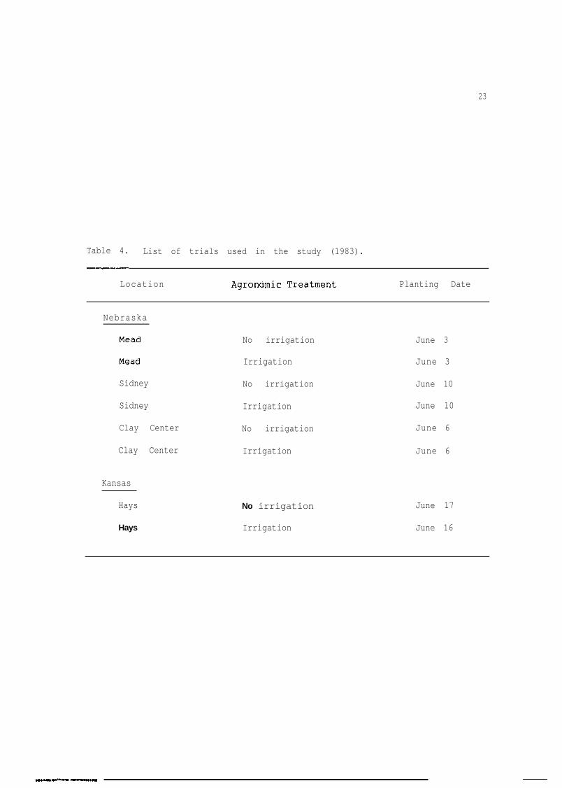
The genotypes were planted at three locations in Nebraska and one
location in Kansas in 1983. Two trials (irrigated and non-irrigated)
were planted at each location. The irrigation treatments were applied
before and after bloom. The amounts of water applied in tQe irrigated
trials were not recorded. In Nebraska, the trials were conducted at the
University of Nebraska Agricultural Field Laboratory, Mead, the High
Plains Agricultural Laboratory, Sidney, and the Agricultural Research
Station, Clay Center. The Kansas location was the Fort Hays Branch
Agricultural Experiment Station, Hays.
The soi1 at Mead was Sharpsburg silt clay loam. Trials at Sidney
were on a Keith silty loam. At C1a.y Center, the trials were on a Hast-
ings s*ilty loam. At Hays, the two trials were planted on different
soils. The irrigated tria1 was on a Roxbury silt loam, while the non-
irrigated tria1 was on a Crete silty clay loam.
The altitude at Mead is 350 m. It is 1800 .m at Sidney, 543 m at
Clay Center, and 579 m at Hays.
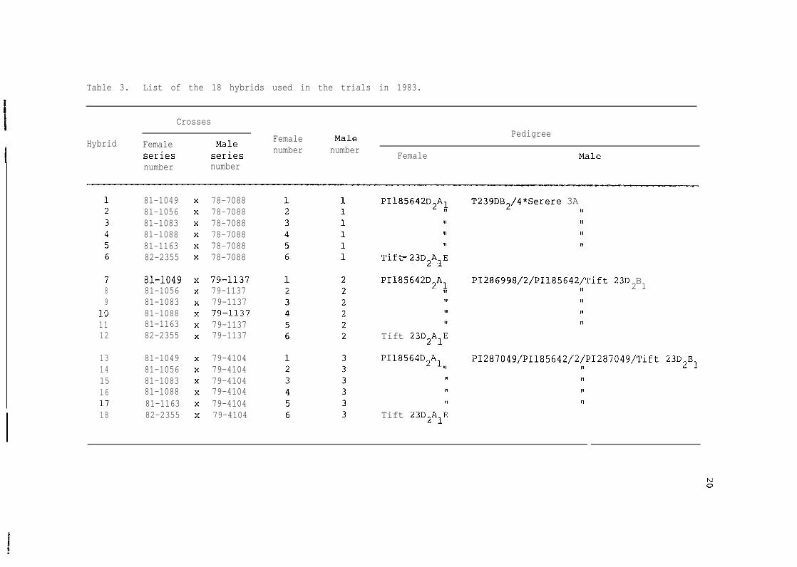
Table 3. List of the 18 hybrids used in the trials in 1983.
Crosses
Female Male PedigreeHybrid Female Male
series series number number Female Malenumber number
81-104981-105681-108381-108881-116382-2355
78-708878-708878-708878-708878-708878-7088
T239DB2/4*Serere 3AIIIIII11
PI185642D2AI
IIIIII
Tift-23D2AlE
PIi85642D2AL PI286998/'2/PIl85642iTift 23D BII 2 1I,1,II
7 8i-iû498 81-10569 81-1083
lû 81-108811 81-116312 82-2355
79-il3779-113779-1137?9-ll??79-113779-1137 Tift 23D2AlE
P118564D2kl,,13 81-104914 81-105615 81-108316 81-108817 81-116318 82-2355
79-410479-410479-410479-410479-410479-4104
PI287049/PI185642/ '2/PI287049/Tift 23D,B,11 L 2.II1111
Tift 23D2AlE

A11 trials received normal. land preparation. The genotypes were
evaluated in a randomized block design with four replications. Some
piots were flooded in the irrigated tria1 at Clay Center. For planting,
a four-row cane planter pulled by a John Deere tractor was used. The
entries were planted in single-row plots with 76 cm between rows. Al1
triais received pre-emergence applications of herbicide (Miloguard).
Except the trials at Hays, no trials received fertilizers. At Hays,
nitrogen fertilizer was applied in the non-irrigated tria1 at the rate
of 45 kg/ha and in the irrigated tria1 at the rate of 30 kg/ha. Al1 the
trials were over-seeded, then thinned to nine plants per meter. The
trials were hand weeded.
The plots were trimmed ta 5 m. Later on, the plots were remeas-
ured before harvest in a11 trials.
The planting date for each tria1 is given in Table 4. Rainfall
and temperature data (Table 5) were recorded for a11 locations.
Plot Eleasurement
Before harvesting, data were collected from each plot in a11
trials, and the following data were taken:
1. Days to half bloom, determined by the number of days from
pianting to flowering date, recorded when 50% of the plants
in the plot had reached half bloom on the main tiller.
2. Plant height, taken from the ground level to the top of the
plants in the plots.
3. Row lengths, measured for each plot.r
23
Table 4. List of trials used in the study (1983).-__-
Location Agronomie Treatment Planting Date
Nebraska
Mead
Mead
Sidney No irrigation
Sidney Irrigation
No irrigation
Irrigation
Clay Center
Clay Center
Kansas
Hays
Hays
No irrigation
Irrigation
No irrigation
Irrigation
June 3
June 3
June 10
June 10
June 6
June 6
June 17
June 16

23
aa,JJ0.rlJJ
1..tvtU
a3.maJ.s
4.
r-im03.F-lCU
a\.2m.u-lcv

24
The plots were harvested after a11 genotypes had reached maturity.
The irrigated tria1 in Hays, the non-irrigated in Mead, and the two
trials in Sidney were harvested and threshed by combine. The remaining
tria& were hand-harvested and threshed by combine. After threshing the
grain from each plot was cleaned and then tested for moisture percentage
in a Burrows digital moisture computer 700. A subsample of each plot
was taken to determine the lOO-seed weight.
Plot grain weight was determined.
From the data taken after harvesting, the following variables
were calculated.
1. Seeds/m2: number of seeds per square meter was computed
as [(Grain weight/plot I plot
x 100.
Plot size (m2) = Row length x
2. Grain yield/ha (kg/ha).
size) i (100-seed weight)l
0.76 m.
Statistical Procedures
The irrigation treatment used in this study differed from loca-
tion to location. Thus, environments were considered as nested within
location. The genotypes in this study are considered fixed effects.
The locations and environments were considered as random.
The analysis of this experiment was subdivided in the following
steps:
a. Individual Experiment Analysis of Variante
The objective of this analysis was to determine the error mean
square for each trial. The error mean squares were tested by the

25
Bartlett test of homogeneity of variante. They were used to calculate
the pooled error mean square for the combined analyses and the stability
analysis.
The following mode1 was used for a:n individual trial:
p =u+rijk i ij i-g +e..ik llk
where:
P th thijk = observation of the k genotype in the j replication
in the i thexperiment.
U i = general mean of the ith experiment.
= effect of the jthr ij replication in the i th experiment.
= effect of the kthg.lk genotype in the ith experiment.
eijk = random error associated with observation of the kth
genotype in the jth repliLation in the i th environment.
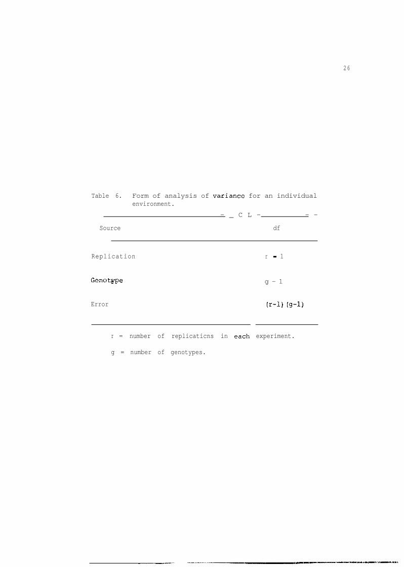
The appropriate analysis of variante is given in Table 6.
b. Combined Analysis
This was computed from the unweighted genotype means as suggested
by Cochran and Cox (1957). The combined analysis provides more informa-
tion about the genotype x environment interaction which cannot be ob-
tained from the individual environment analysis. It was computed over
replications.
The following mode1 was used:
Fijk =u+l -i + e(l) ji + gk ,f (gl) ki + (ge(l.1) kji ' eijk
26
Table 6. Form of analysis of variante for an individualenvironment.
- _ C L - - -
Source df
Replication r - 1
Genotvpe g - 1
Error (r-1) (4-l)
r = number of replicaticns in each experiment.
g = number of genotypes.

27
where:
F.1jk
U = general mean of the experiments.
li = effect of the ith location.
e(l) ji = effect of the jth environment within the i th
'k
(gl)ki
= mean of the kth genotype in the jth environment in
the location.
location.
= effect of the k th genotype.
= interaction effect of the kth genotype with the
i th location.
ige(l) ) k j i
= interaction effect of the k th genotype with j th
environment in the i th location.
ëijk = random error associated with the k th genotype mean
at the j th environment in the i th year.
The appropriate form of analysis of variante is given in Table 7.
The components of variante for the interaction effects along with
their standard errors were also calculated as follows:
Components of variante:
a2ge/l = M2 - Ml
ô291 = (M3 - M2)/e
Standard errors:
S.E. (â2ge/l) =[2M22 2M21
(df2 + 2) + (dfl -'-$
+ 2)

dfMean square F
Observed Expected
Location (L) l-1
Environment within 1location (E/L) z(ei-
i=l
Genotypes (G 1
GXL
G x E/L
Pooled error
g-1 M4 2 2 2 -2ue,n + ugell + wge + eU(gk-g) M /M
4 3(g-1)
(g-1) (1-l i2
M32 2
'e/n + 'ge/l + eagl M /M3 2
(g-1) E cei-ll*:
(g-1) i(r. -1)i=l 1
2 2M2 'e/n + oge/l
2Ml 'e/n
M2'M1
1 = number of locations. e = number of genotype.e = number of environments within locations. r = number of replications per experiment.n = harmonie mean of the number of replications. P = number of experiments.
n = P/C(l/ri)where:
P = number of experiments. thr.1 = number of replications in the i experiments.
+ The pooled error mean square for the combined analysis was calculated from the formula:
Pooled error mean square = Iwhere:
CSz/rP i
P = number of experiments.
S 2i = errer mean square of the i th experiment.
thr. = number of replications in the i experiment.1
29
S.E. (G22M2 3 2M2
gl) =l/ef2 ;
Kif3 + 2)
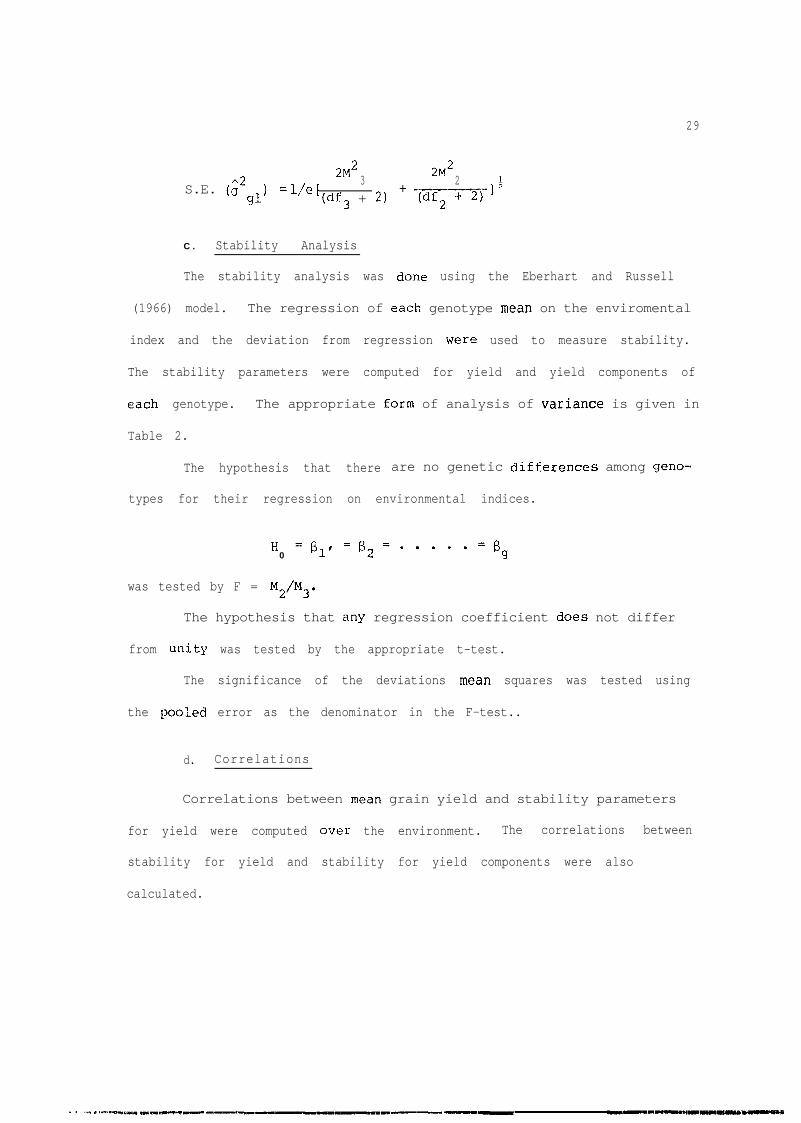
C . Stability Analysis
The stability analysis was done using the Eberhart and Russell
(1966) model. The regression of each genotype mean on the enviromental
index and the deviation from regression 'were used to measure stability.
The stability parameters were computed for yield and yield components of
each genotype. The appropriate form of analysis of variante is given in
Table 2.
The hypothesis that there are no genetic differences among geno-
types for their regression on environmental indices.
H =B,,=fj,=.....=B0 g
was tested by F = M2/M3.
The hypothesis that any regression coefficient does not differ
from unity was tested by the appropriate t-test.
The significance of the deviations mean squares was tested using
the pooled error as the denominator in the F-test..
d. Correlations
Correlations between mean grain yield and stability parameters
for yield were computed over the environment. The correlations between
stability for yield and stability for yield components were also
calculated.
- .. ” .-__“_l.l.,._ __.II.-_-- P------P- -- -- ---*1141-.1uL1IIII1)*c

3 0
Al1 these analyses were done on the Nebraska University Remote
Operating Station (N.U.R.O.S.) at the University of Nebraska, L,incoln,
using S.A.S. 1 The analyses of variante for the individual experiments
were done with the GLM procedure and for the combined analysis over
environments with PROC ANOVA. The regression analysis was done with
the E'ROC REG procedure and the correlations with PROC CORR procedure.
--
1 Statistical Analysis System. Description available from SASInstitute, Inc., Box 8000, Cary, North Carolina 27511.
- . II._. _II ._“-- _ -.-,*,, “_ ---,_------------------- .._I_ -.----~-.<“-,-~~-~,~--

RE:SULTS
The environment mean yield for al:L hybrids ranged from 464 kg/ha
in Hays (non-irrigated) to 3333 kg/ha in Clay Center (irrigated) (Table
??? ? Mean days to 50% bloom ranged from 60 days to 71 days, mean plant
height from 81.6 cm to 127.6 cm, mean lOO-seed weight from 0.88 g to
1.24 g, and mean number of seeds from 4828 to 26,329 (Table 8).
The average growing season temperatures ranged from 13.8OC at
Sidney to 25.3OC at Hays and the total growing season moisture received
from 3.8 cm in Sidney to 31.1 cm in Clay Center (Table 5).
The diversity among environment means and the range in environ-
mental factors provided a good opportunity to study for genotype x
environment interactions and stabihity.
Genotype x Environment Interaction
The combined analysis considered t.he variation due to hybrid,
hybrid x location, and hybrid x environment within location. The com-
ponents of variante for each of the above effects were estimated from
the combined analysis to assess the importance of the different
interactions.
The combined analysis of variante (Table 9) shows a significant
difference among the means of the hybrids for days to 50% bloom plant
and height and seeds/m2. The hybrid means for seed weight were not sig-
nificantly different. The comparisons among means (Table 14) showed a
difference in seed weight among the hybrids.

Table 8. Environment means for the different traitsr
TraitLocation Environment Days to
50% bloomPlantheight
100-seedweight Seeds/m2 Grain Yield
(days 1 (cm) (9) (number) (W'ha)
Mead non-irrigated
irrigated
62.7 112.4 1.13 10,126 1,208
63.4 127.6 la24 21,245 3 777-, , , ,
Sidney non-irrigated 68.5 107.7 1.04 16,479 1,784
irrigated C;R "V.d 7 .A."V. 1nQ 4 0.99 16 6,75 1,713
Clay Center non-irrigated 63.0 106.1 1.19 20,111 2,522
irrigated 64.5 123.4 1.21 26,329 3,333
Hays non-irrigated 70.5 81.6 0.88 4,828 464
irrigated 59.8 125.1 1.07 25,340 2,801

Table 9. Comblned analysis of variante for the 18 millet hybrids.
Mean square
Source df Days to Plant 100-seed50% bloom height weight Seeds/m' Grain yield
tdays 1 (cm) (9) (number) (Wha)
Location (L) 3 202.57 1,942.65 0.4962 510,467,188 12,443,137
Environment/location (E/L) 4 266.00 5,446.39 0.1128 1,311,9?9,11? 'Q 1'4,6'89--',-'A
Fiybrid (H) 17 19.08** 183.17** 0.0965 15,559,106* 576,694**
HxL 51 1.99** 26.25** 0.0028 8,017,627 93,921*
H x E/L 68 0.92 14.23 0.0029* 5,741,791 59,681
Pooled error 394 1.02 11.30 0.0020 5,172,520 65,845
* and ** indicate significance at the 0.05 and 0.01 levels, respectively.

34
The hybrid x location mean square indicated significant differ-
ences for grain yield (0.05 level), 9lan.L height, and days to 50% bloom
(0.01 level). The differences among hybrids were consistent for 100-
seed weight and seeds/m' across locations.
The hybrid x environment within location mean squares were sig-
nificant (0.05 level) for lOO-seed weight. For the other traits, the
differences among hybrids were consistent across environment within
location.
The magnitude of the components of variante gives information
about the importance of the different interactions. The estimates of
the components of variante for a11 traits are given in Table 10. For
days to 50% bloom, the component of variante of hybrid x location was
higher than for hybrid x environment within location. The same pattern
also was found for plant height, grain yield, and seeds/m'. The results
showed that for grain yield and days to 50% bloom, the estimate of
A2*I#/L was negative and less than the S.E,, and thus it cari be considered
equal to zero. The component of variante for hybrid x environment
within location was higher for lOO-seed weight.
Stability Analysis
The stability anaiysis was performed with a11 hybrids over the
eight environments. It provides an estimate of the linear regression
(b) and mean square deviations from regression (Sd) for each hybrid.
Stability Analysis of Variante
The results in Table 11 show that hybrid x environment interac-
tion was significant for a11 traits except grain yield.


Table 11. Stability analysis of variante for the 13 millet hybrids.
Mean square
Source df Days to Plant 100-seed50% bloom height weight Seeds/m2 Grain Yield
Hybrid x Environment
Environment (linear)
Hybrid x Environment(linear)
Pooled deviations
Pooled error
(days 1 (cm) (9) (number)
119 1.38** 19.44** 0.0028"" 6,717,149*
1 1,671.74 27,613.51 193.99 6,779,318,036
17 1.70 30.32** 0.0075* 8,307,957
108 1.25 16.-64** 0.0020 6,093,565
394 1.02 11.30 0.0020 5,172,520
(kg/ha)
74,356
114,552,768
85,848
68,414
65,845
* and ** indicate significance at the 0.05 and 0.01 levels, respectively.
37
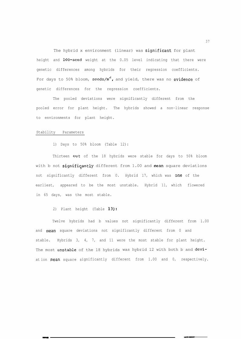
The hybrid x environment (linear) was significant for plant
height and 100-seed weight at the 0.05 level indicating that there were
genetic differences among hybrids for their regression coefficients.
For days to 50% bloom, seeds/m‘( and yield, there was no evidence of
genetic differences for the regression coefficients.
The pooled deviations were significantly different from the
pooled error for plant height. The hybrids showed a non-linear response
to environments for plant height.
Stability Parameters
1) Days to 50% bloom (Table 12):
Thirteen out of the 18 hybrids were stable for days to 50% bloom
with b not signifi~antly different from 1.00 and mean square deviations
not significantly different from 0. Hybrid 17, which was one of the
earliest, appeared to be the most unstable. Hybrid 11, which flowered
in 65 days, was the most stable.
2) Plant height (Table 131:
Twelve hybrids had b values not significantly different from 1.00
and mean square deviations not significantly different from 0 and
stable. Hybrids 3, 4, 7, and 11 were the most stable for plant height.
The most unstable of the 18 hybrids was hybrid 12 with both b and devi-
at ion mean square significantly different from 1.00 and 0, respectively.

38
Table 13. Stability parameters of the 18 hybrids for days to 50% bloom.
-.--cc
Iîybrid Mean bi MSD+j- R2- - - -
(days 1
123456789
101112131415161718
Mean
63.4 h65.6 cde64.8 ef64.0 fgh63.3 hi62.3 i66.1 cd69.4 a66.2 bcd67.2 b64.9 ef66.6 bc65.3 de66.3 bcd65.3 de64.6 efg63.6 gh64.1 fgh
65.1?'
0.98 0.95 0.94 s1.03 0.72 0.96 s1.07 0.93 0.93 s1.22 0.98 0.831.01 1.23 0.75 s0.92 0.41. 0.92 s1.00 2.76 0.91 s0.71** 1.68 0.921.15 0.42 0.92 s0.98 1.52 0.97 s0.97 0.38 0.89 s0.83 3.48** 0.971.23* 0.74 0.871.09 0.56 0.96 s1.00 1.44 0.88 s1.06 0.40 0.95 s0.78* 2.20" 0.450.96 1.78 0.84 s
--1_
Means followed by the same letter are not significantly different atthe 0.50 level.
-t * and ** indicate significant difference from 1.00 at the 0.05 and0.01 levels, respectively.
"r-t* and‘** indicate significant difference from 0 of the 0.05 and 0.01levels, respectively.
s = Stable. A stable hybrid is the one with b net significantly dif-ferent from 1.00 and mean square deviations (MSD) not signifi-cantly different from 0.

39
Table 13. Stability parameters of the 18 hybrids for plant height.
Hybrid Mean bt MSD-I-i' R2
(cm)
1 111.10 def 0.94 15.202 111.57 de 1.13 25.98"3 113.06 cd 0.97 9.884 110.63 dcf 1.00 9.095 108.51 efg 0.84 16.026 118.06 b 1.19 24.16*7 116.06 bc 0,97 8.898 113.51 cd 1,23* 14.569 117.52 b 0.96 12.04
10 112.22 de 1.03 2.7611 111.44 de 0.92 9.8412 121.62 a 1,34** 34.39**13 107.51 fgh 1.04 13.2114 106.77 gh 0,86 24.ci9*15 106.16 gh 0.93 17.0616 104.69 h 0,96 21.9917 104.71 h 0.79* 27.55*18 113.16 cd 0.92 12.29
Mean 111.57
0.93 s0.920.96 s0.96 s0.92 s ,0.940.96 s0.960.95 s0.99 s0.96 s0.930.95 s0.880.93 s0.91 s0.850.95 s
Means followed by the same letter are not significantly different atthe 0.05 level.
+* and ** indicate significant difference from 1.00 at the 0.05 and0.01 levels, respectively.
i-t* and ** indicate significant difference from 0 at the 0.05 and 0.01levels, respectively.
s = Stable. A stable hybrid is .the one with b net significantly dif-ferent from 1.00 and mean square deviations (MSD) not signifi-cantly different from 0.
40
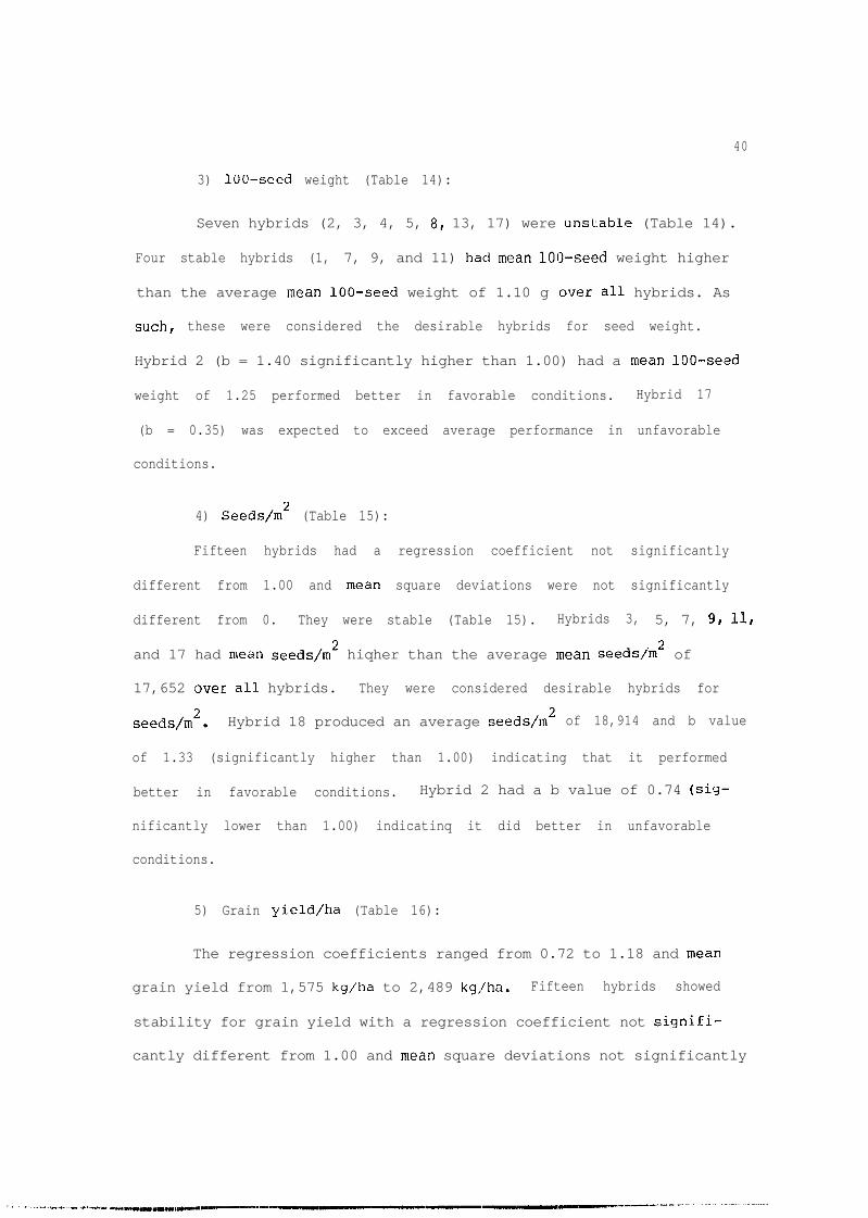
3) 100-seed weight (Table 14):
Seven hybrids (2, 3, 4, 5, 0, 13, 17) were unstable (Table 14).
Four stable hybrids (1, 7, 9, and 11) hacl mean 100-seed weight higher
than the average mean lOO-seed weight of 1.10 g over a11 hybrids. As
such, these were considered the desirable hybrids for seed weight.
Hybrid 2 (b = 1.40 significantly higher than 1.00) had a mean lOO-seed
weight of 1.25 performed better in favorable conditions. Hybrid 17
(b = 0.35) was expected to exceed average performance in unfavorable
conditions.
4) Seeds/m2 (Table 15):
Fifteen hybrids had a regression coefficient not significantly
different from 1.00 and mean square deviations were not significantly
different from 0. They were stable (Table 15). Hybrids 3, 5, 7, 9, 11,
and 17 had mean seeds/m2 hiqher than the average mean seeds/m2 of
17,652 over a11 hybrids. They were considered desirable hybrids for
seeds/m2. Hybrid 18 produced an average seeds/m2 of 18,914 and b value
of 1.33 (significantly higher than 1.00) indicating that it performed
better in favorable conditions. Hybrid 2 had a b value of 0.74 (sig-
nificantly lower than 1.00) indicatinq it did better in unfavorable
conditions.
5) Grain yield/ha (Table 16):
The regression coefficients ranged from 0.72 to 1.18 and mean
grain yield from 1,575 kg/ha to 2,489 kg,/ha. Fifteen hybrids showed
stability for grain yield with a regression coefficient not signifi-
cantly different from 1.00 and mean square deviations not significantly

41
Table 14. Stability parameters of the 18 hybrids for lOO-seed weight.- -
Wybrid Mean b-t MSDtt R2---
(9)
1 1.26 a 1.17 0.00232 1.25 a 1.4o'k* 0.00163 1.24 a 1,32* 0.00254 1.19 b l-14 0.0046"5 1.19 b 0.73 0.00316 0.97 g 0.93 0.00137 1.11 cde 0.96 0.00178 1.09 cde 1,36** 0.00299 1.12 cd 0.90 0.0012
10 1.03 f 1.15 0.000811 1.12 cd 0.77 0.001312 0.88 h 1.11 0.000713 1.07 def 1.18 0.0046X14 1.09 cde 1.01 0.000815 1.07 def 0.83 0.001616 1.07 def 0.89 0.000717 1.12 cde 0.35** 0.002718 0.87 h 0.76 0.0019
Mean 1.10
0.91 s0.960.930.830.750.92 s0.91 s0.920.92 s0.97 s0.89 s0.97 s0.8d0.96 s0.88 s0.95 s0.450.84 s
Means followed by the same letter are not significantly different att:he 0.05 level.
t* and ** indicate significant difference from 1.00 at the 0.05 and0.01 levels, respectively.
tt* and ** indicate significant difference from 0 at the 0.05 and 0.01.levels, respectively.
s = Stable. A stable hybrid is the one with b not significantly dif-ferent from 1.00 and mean square deviations (MSD) not signifi-cantly different from 0.

42
Table 15. Stability parameters of the 18 hybrids for seeds/m2.- -
Hybrid Mean b-t MSDj-t R2 -
1 16,213 def 0.882 18,312 bcde 0.74*3 18,758 abcd 0.854 17,178 abcdef 1.025 19,277 ab 1.156 19,614 a 1.217 18,365 abcde 1.098 15,995 ef 0.959 19,029 abc 0.99
10 16,179 def 0.9511 18,780 abcd 1.1812 16,706 bcdef 0.9113 15,927 ef 0,9314 16,565 cdef 0.8515 17,541 abcdef 0.9016 15,328 f 0.9717 19,056 abc 1.0718 18,914 abc 1*33'k*
(number)
7,199,50212,193,275*2,696,6263,261,6072,458,368
13,016,728*1,371,6897,985,7055,717,3846,235,0441,079,601
1 5,563,8141,923,8162,505,6208,888,7171,113,8094,917,419
21,555,525**
0.87 s0.740.94 s0.95 s0.98 s0.870.98 s0.88 s0.91 s0.90 s0.99 s0.90 s0.96 s0.95 s0.85 s0.98 s0.94 s0.84
Mean 17,652
Means followed by the same letter are not significantly different atthe 0.05 level.
j-* and *E indicate significant difference from 1.0 at the 0.05 and0.01 levels, respectively.
-f-t* and ** indicate significant difference from 0 at the 0.05 and0.01 levels, respectively.
s = Stable. A stable hybrid is the one with b not significantly dif-ferent from 1.00 and mean square deviations (MSD) not signifi-cantly different from 1.

43
Table 1G. Stability parameters of the 18 hybrids for grain yield.
-
Hybrid Mean b-t MSDtt lx2
(b/ha)
1. 2,182 bcd 1.03 88,216l! 2,483 a 0.99 220,140*X3 2,489 a 1.06 48,0514 2,213 abcd 1.16 20,855Ei 2,408 ab 1.16 34,7606 2,052 cde 1.12 123,8097 2,198 abcd 1.09 24,6298 1,898 ef 0.95 122,9949 2,283 abc 1.02 69,758
10 1,810 efg 0.96 81,28211. 2,263 abc 1.18* 23,32712 1,575 g 0.72** 38,64813 1,847'efg 0.90 41,12714 1,932 def 0.88 18,463151 2,024 cde 0.93 97,75716 1,774 efg 0.93 21,62617 2,194 bcd 0.98 50,00018 1,728 fg 0.93 102,004
0.93 s0.830.96 s0.98 s0.98 s0.91 s0.98 s0.89 s0.94 s0.92 s0.980.980.95 s0.98 s0.90 s0.98 s0.95 s0.90 s
Mean 2,075
c- -
Means followed by the same letter are not significantly different atthe 0.05 level.
t* and ** indicate significant difference from 1.00 at the 0.05 and0.01 levels, respectively.
-f-t* and ** indicate significant difference from 0 at the 0.05 and0.01 levels, respectively.
s = Stable. A stable hybrid is the one with b mot significantly dif-ferent from 1.00 and mean square deviations (MED) not signifi-cantl.y different from 0.

44
different from 0 (Table 16). Hybrids 1, 3, 4, 5, 7, 9, and 17 yielded
higher than the average yield of 2,075 kg/ha over a11 hybrids. They
were the desirable hybrids for grain yie.Ld. Hybrid 3 which had the
highest yield (2,489 kg/ha) was the most desirable.
Figure 1 shows the response of three stable hybrids (5, 7, 14) to
environmental indices. Hybrid 5 (b = 1.16) produced better in more
favorable environments, and its performance was consistent. Hybrid 14
with b = 0.88 was expected to perform better in unfavorable environments.
Based on the RL (coefficient of determination) which measures
the magnitude of the non-linear response and similar to the deviation
mean square, only hybrid 2 was unstable (RL = 0.83).
The average regression coefficient and deviation mean square for
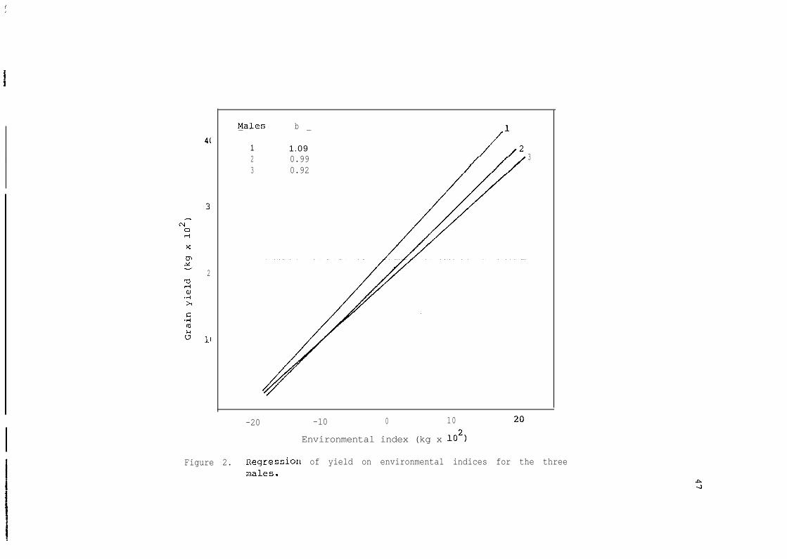
each male are given in Table 17. Al1 males were stable. Figure 2 shows
the linear response of the three males to environments. Male 1 per-
formed better in high yielding environments, and male 3 was expected to
do relatively well in low yielding envir'onments. Male 1 which yielded
on the average higher than the average yield of a11 males was consid-
ered as desirable.
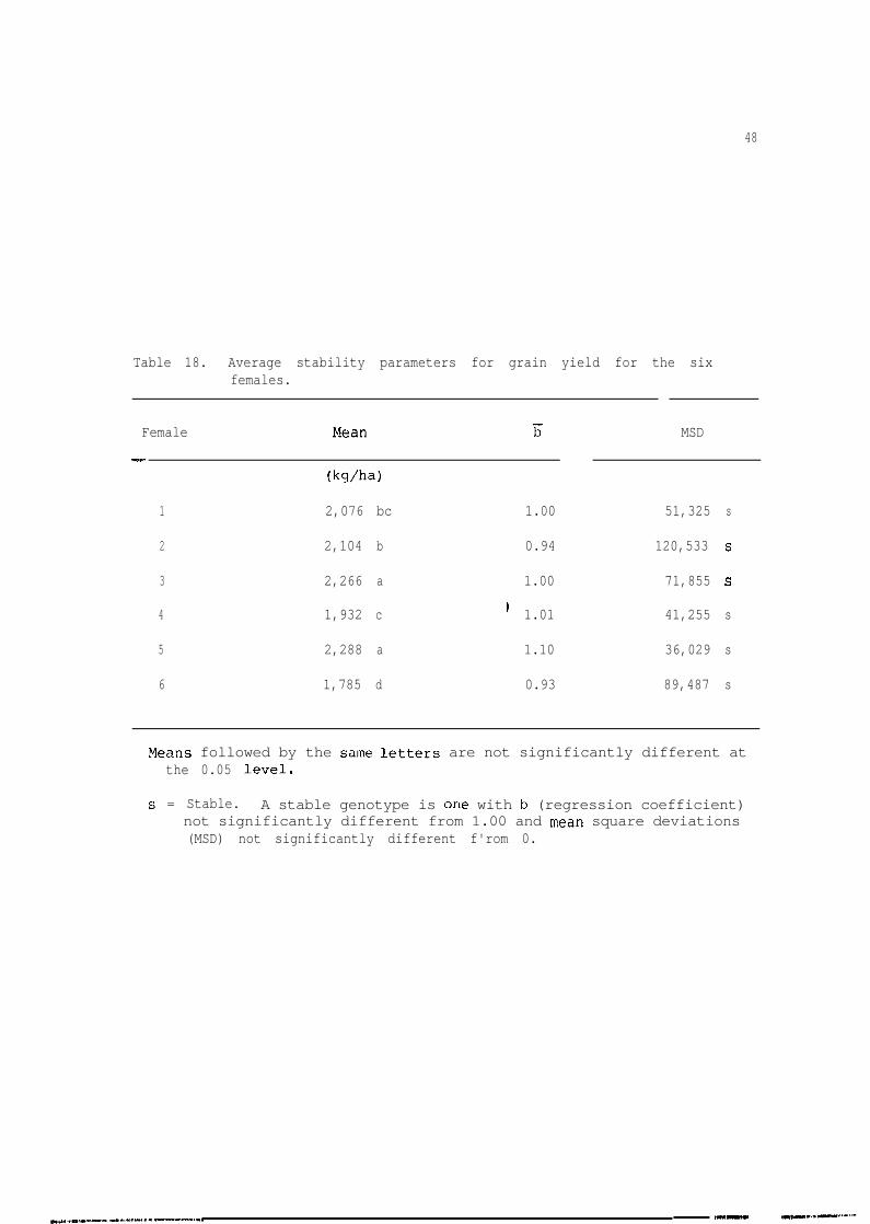
On the other hand, the regression coefficients and deviation mean
squares of each female (Table 18) showed that a11 females were stable.
Figure 3 shows the average response of three females to varying environ-
ments. Female 5 is expected ta do better in favorable environment
conditions, while female 6 is expected to equal or exceed the average
performance only in unfavorable conditions (b = 0.93 and mean = 1,785
kg/ha).

4 5

46
Table 17. Average stability parameters for grain yield of the threemales.
Male.I_-
Mean b MSD
1 2,305 a 1,09 89,310 s
2 2,004 b 0.99 60,107 s
3 1,917 b 0.92 55,829 s
Means followed by the same letters are not significantly different atthe 0.05 level.
s = Stable. A stable genotype is the one with b (regression coeffici-ent) not significantly different from 1.00 and mean square devi-ations (MSD) not significantly different from 0.
4(
31
2
II
Males b- -
1 1.092 0.99 33 0.92
-20 -10 0 10
Environmental index (kg x 102)
Figure 2. Regression of yield on environmental indices for the threemales.
48
Table 18. Average stability parameters for grain yield for the sixfemales.
Female-
1
2
3
4
5
6
Mean
(Wha)
2,076 bc
2,104 b
2,266 a
1,932 c
2,288 a
1,785 d
TT MSD
1.00 51,325 s
0.94 120,533 s
1.00 71,855 s
' 1.01 41,255 s
1.10 36,029 s
0.93 89,487 s
Means followed by the same letters are not significantly different atthe 0.05 level.
s = Stable. A stable genotype is one with b (regression coefficient)not significantly different from 1.00 and mean square deviations(MSD) not significantly different f'rom 0.

-20 -10 0 J"O
Environmental index (kg x 102)
20
Figure 3. Regression of yield on environmental indices for three females.
50
Relationship Between Mean Yield Performance and Stability Parameters- - - - -
The correlation between hybrid means and stability parameters
(11, Si:) was determined. Mean yield was significantly and positively
correlated with the regression coefficient for yield (r = 0.73).
Therefore, the genotypes used tended to have high yields along with
large regression coefficient.
On the other hand, there was a low correlat.ion bet.ween mean yield
and S2tu (r = 0.15). Since the association between mean yield and Sd for
yield was not significant, the two traits could be selected independ-
ently, i.e., selection of high yielding genotypes with low mean square
deviations.
Relationship Between Stability Parameters and Coefficient of- -
1 Determination (R2)
The correlation between reg:ression. coefficients and coefficient
of determination was not significant (r =: 0.30). The correlation
between R2 and Si was significant (r = -0.95) . When stability of
genotype is assumed to measure how well the actual. yields of the geno-
types are predicted, the result suggested that R2 should be a satisfac-
tory parameter for measuring stability. However, it does not give any
information about the responsiveness of t.he genotype as shown by the 10w
correlation with b.
Relationship Between Stability for Yield and Stability for Yield- -
Components- -
Correlation coefficients among the stability parameters for grain
yield and stability parameters for yield components are given in Table
51
19. A significant correlation was found between mean grain yield and
mean 100-seed weight (r = 0.83) and mean seeds/m' (r = 0.54). This
indicates that yield was dependent on seed weight and seeds/m2. There
was also a significant correlation between the regression coefficient of
grain yield and the mean seed weight and seeds/m2. A significant and
negative correlation was found between b for yield and Sd for plant
height indicating that low mean square deviations for plant height
enhances the response of millet to high Iyielding environments. There
was also a significant positive correlation between Sd for grain yield
and C 2 .Lad for seeds/m2 indicating that the stability for seeds/m2 was
related to the stability of grain yield. Correlations between grain
yield stability parameters and those of Idays to 50% bloom were negative
but were not significant. Thus, grain yield seems to increase when
number of days to 50% decreases.
The results suggested that stability of grain millet yield was
mostly rekated to the stability of seeds,/m2, while the overall yield
production depends mostly on mean seed weight.
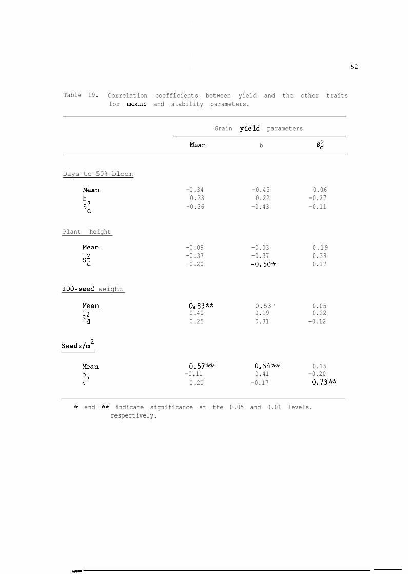
Table 19. Correlation coefficients between yield and the other traitsfor means and stability parameters.
Grain yield parameters
Mean b 4
Days to 50% bloom
Meanb
SS
-0.34 -0.45 0.060.23 0.22 -0.27
-0.36 -0.43 -0.11
Plant height
Mean -0.09 -0.03 0.19b -0.37 -0.37 0.39sd -0.20 -0.50* 0.17
lOO-seed weight
Mean Or83** 0.53" 0.05b 0.40 0.19 0.22sd 0.25 0.31 -0.12
Seeds/m2
Mean 0.57** 0.54** 0.15-0.11 0.41 -0.200.20 -0.17 0,73*-k
* and ** indicate significance at the 0.05 and 0.01 levels,respectively.

DISCUSSIO:N
Genotype x Environment Interaction- -
The yield trials were conducted at four locations in 1983 to
evaluate the genotype x environment interactions for 18 millet hybrids.
At each location, two experiments were planted. This gives eight envi-
ronments. The analysis of the individual experiments showed that the
individual error variantes were not homogeneous, but the pooled error
mean square from individual experiments appears to be the best estimate
of error variante for the combined analysis whether the individual error
variante are homogeneous or not. According to Cochran and Cox (1957),
the heterogeneity of variantes lead to too many significant results.
Therefore, the relative magnitudes of the interaction components of
variante are more important than their significance. The estimates
the interaction components of variante, hybrid x environment within
I
of
location (G2HE/L) ' and hybrid x location A2I:o HL ) were obtained from the
combined analysis.
A2The relatively large rsHE,L for 100-seed weight indicates that
the relative performance of the hybrids ccross environments within a
locat.ion was more inconsistent than across location for the trait. The
A2%L was higher than â2HE/L for days to 50% bloom, plant height, grain
yield, and seeds/m2 suggesting that the performance of the hybrids was
more inconsistent across locations. Thus, to reduce the magnitude of
the interaction for the traits, the testing area should be divided into
subregions.

54
From the results, it appears that millet responds differently to
environments, and the hybrid x environment within a location interaction
was more important for 100-seed weight, but for grain yield, plant
height, days to 50% bloom, and seeds/m2, the hybrid x location inter-
action was more important.
Grain Yield and Components Stability- -
It is commonly observed that the relative performance of differ-
ent genotypes varies in different environments, i,e., there is a geno-
type x environment interaction which has been a challenge to fully
understand the control of variability. The genetic variability is
inferred from the phenotype.
and stable genotypes becomes
program.
Therefore, screening for high yielding
an important part of the plant breeding
l
The study was based on 18 hybrids grown in different environ-
mental conditions. The Eberhart and Russell (1966) method was used for
the stability analysis by estimating the linear regression (b) and the
mean :square deviations from regression (Sd). Linear regression (b)
shows the response of a genotype to varying environments, while S d
measures the dispersion around the regression line, i.e., how well the
predicted response agrees with the observed. Eberhart and Russelln
(1966) considered Si to be the best measure of stability. A genotype
with b value not significantly different from 1.00 and mean square
deviations from regression not significantly different from 0 or as
small as possible was considered as stable. A stable genotype Will be
more desirable when it has a mean yield greater than the average yield
of all genotypes.

55
The hybrid x environment mean square was siynificant for a11
traits except for grain yield indicating that the performance of the
hybrid varies with environment. There was no hybrid x environment
interaction for grain yield. The ILack of interaction for grain yield
was expressed by the large number of stable hybrids. Fifteen out of 18
hybrids were stable. Seven hybrids were desirable. The absence of
interaction might be related to the fact that the environments did not
represent an extremely wide diversity in environmental conditions. For
the other traits, although there was a sizable hybrid x environment
interaction, more than half of the hybrids were stable. This indicates
that more testing is required in order to have precise information on
the stability of the hybrids for plant height, days to 50% bloom,
lOO-seed weightj and seeds/m2.
The average regression caefficient and mean square deviations
from regression for yield of the males an'd the females indicate that a11
parents were stable. This suggests that almost a11 parents could be
used as parents in crosses for yield stability.
The significance of the correlation between
regression coefficient for yield indicates that it
mean yield and the
is possible to have
high yielding hybrids in favorable conditions. The yield of millet
genotypes increases when environmental conditions improve. Similar
results were reported by Eagles et al. (1977) in oats and by Busch et
al.. (1976) in wheat. The two traits are dependent, and selection for
high response to environments Will enhance grain yield.
The coefficient of determination (R2) for yield was negatively
and significantly correlated with the mean square deviation from regres-
sion (Sd) indicating that II2 could be used for assessing the predicta-

56
bi1it.y of yield. High Ft2 Will indicate :Low nonlinear response. The
contribution of various plant traits to yield stability is of interest
to plant breeders. The finding of traits associated with yield allows
the selection for yield stability through these traits. The mean square
deviations from regression for seeds/m' was significantly correlated to
the mean square deviations of yield. Selection of hybrid with low mean
square deviations for seeds/m2 appears to improve the stability of yield.
Mean 100-seed weight and mean seeds/m2 were positively and significantly
correlated to mean yield. It suggests that both lOO-seed weight and
seeds,/m2 determine the yielding potential of the millet hybrids. On the
other hand, high responsive hybrids in favorable conditions produce
heavier seeds, (r = 0.53) and more seeds/m2 (r = U.54). Egharevba et
1 al. (P983) found no significant correlation between weight of seeds and
yield in millet. The existence of interaction may have caused the high
correlation found in this study. The association between deviation mean
square for plant height and regression coefficient for grain yield is
not readily interpretable without knowledge about the relationship
between plant height and yield. According ta Egharevba et al. (1983),
there was a positive correlation between the two characters, but they
concluded that there was no evidence that taller plants were more effi-
tient than shorter plants in grain produc,tion.
Since the development of yield components is a series of sequen-
tial events, stress due to environmental factors at any stage might
affect the final yield. Therefore, compensation for reduction of one
component with an increase in another may be important for yield
stability. .

SUMMARY
The stability of 18 millet hybrids was studied in eight environ-
ments across Nebraska and Kansas using the Eberhart and Russell (1966)
method. The objectives of the study were (1) to investigate the impor-
tance of genotype x environment interaction in a millet testing program;
(2) to estimate stability parameters for each hybrid and identify stable
hybrids for days to 50% bloom, plant height, 100~seed weight, seeds/m2,
and yield.
The relative magnitude of the components of variante due to
hybrid x environment within location and hybrid x location indicated
that interaction of hybrids with location was more important for grain
yield, days to 50% bloom, plant height, and seeds/m2. The relative
magnitude of the components of variante showed that interaction of
hybrid with environments within a location dominated for lOO-seed
weight. The reaction of the hybrids to location OK environment within
location changes depending on the measured traits, i.e., on the sensi-
tivity of the traits to change in conditions across locations or across
environments with a location.
The hybrid x environment interaction was not significant for
grai.n yield. Thus, more than 2/3 of the hybrids were stable for grain
yield. Testing in a wider range of environmental conditions is needed
before concluding about the general adaptation of the hybrids.
Grain yield was associated with seed weight and seeds/mL. HOw-
ever, it was correlated higher with seed veight than to seeds/m2. The
statility of the hybrids for grain yield across environments was related
.I. I ,D~<, >/“..” .r - ” ._,_ _._.__..“.._ _-_. IC~““,C-------III---mœwmmem,1”*-<---

58
to the stability in seeds/m2. Thus, selection for stability of grain
yield cari be done through seeds/m2.
The full assessment of yield components to find those mostly
related to stability of yield requires a broad investigation on a11
traits affecting yield over environments.
LITERATLJRE CITED
Allard, R.W. 1961. Relationship between genetic diversity and con-sistcncy of performance in different environments. Crop Sci.1: 127-133.
Allard, R.W., and A.D. Bradshaw. 1964. Implications of genotype-environment interaction in applied plant breeding. Crop Sci.4: 503-507.
Breese, E.B. 1969. The measurement and significance of genotype-environment interactions in grasses. Heredity 24: 27-44.
Busch, R.H., J. Hammond, and R.C. Frohberg. 1976. Stability and per-formance of hard red spring wheat bulks for grain yield. CropSci. 16: 256-258.
Cochran, R.E., and G.M. Cox. 1957. Experimental ~designs. John Wileyand Sons, Inc., New York.
Eagles, H.A., P.N. Hinz, and K.J. Frey. iL977. Selection of superiorcultivars of oats by using regression coefficients. Crop Sci.17: 101-105.
Eberha.rt, S.A., and W.A. Russell. 1966. Stability parameters forcomparing varieties. Crop Sci. 6: 36-42.
Eberhart, S.A., and W.A. Russell. 1969. Yield and stability for lO-lines diallel single crosses and double crosses maize hybrids.Crop Sci. 9: 357-361.
Egharevba, P.N., A.A. Ibrahim, and A.A. Okolo. 1983. Some morphologi-cal and physiological determinants of grain yield in Pearl millet.Maydica 28: 15-24.
Francis, T-R., and L.W. Kannenberg. 1978. Yield stability studies inshort season maize. A descriptive method for grouping genotypes.Can. J. Plt. Sci. 58: 1029-1034.
Finlay, K.W., and G.M. Wilkinson. 1963. The analysis of adaptabilityin plant breeding programme. Aust. J. Agric. Res. 14: 742-754.
Fi&er, R.A., and W.A. Mackenzie. 1923. Studies in trop variation.II. The manual response of different potato varieties. J. Agric.Sci. Camb. 13: 311-320.
Freeman, G.H., and J.M. Perkins. 1971. Environmental and genotype-environmental components of variability. VII. Relations betweengenotypes grown in different environments and measures of theseenvironments. Heredity 27: 15-23.

6 0
Fripp, Y.J. 1972. Genotype-environmental interactions in Schizophyllumcommune. 11. Assessing the environments. Heredity 28: 223-238.
Hardwick, R.C., and J.T. Wood. 1972. Regression methods for studyinggenotype-environment interactions. Heredity 28: 209-222.
Heinrich, G.M. 1981. Morphological and physiological mechanisms ofyield stability in grain so.rghum (Sorghum bicolor [L.] Moench)across diverse environment. Ph.D. Dissertation, University ofNebraska, Lincoln, NE.
Horner, T.W., and K.J. Frey. 1957. Methods of determining naturalareas for oat varietal recommendations. Agron. J. 49: 313-315.
Jensen, N.F. 1952. Intravarietal diverification in oat breeding.Agron. J. 44: 30-34.
Jinks, J.L., and J.M. Perk-ins. 1970. Environmental and genotype-environmental components of variability. VII. Simultaneous pre-dictions across environments and generations. Heredity 25: 419-429.
Jones, D.F. 1958. Heterosis and homeostasis in evaluation and appliedgenetics. Am. Nat. 92: 321-328.
Joppa, L-R., K.L. Lebsock, and R.H. Busch. 1971. kield stability ofselected spring wheat cultivars (Triticum aestivum L. en Thell)in uniform regional nurseries, 1939 to 1968. Crop Sci. 11:238-241.
Jowett, D. 1972. Yield stability parameters for sorghum in EastAfrica. Crop Sci. 9: 359-361.
Langer, I., K.J. Frey, and T. Bailey. 1979. Associations among pro-ductivity, production response and stability indices in oatsvarieties. Euphytica 28: 1'7-24.
Lewis,, D. 1954. Gene-environment interaction. A relationship betweendominanceF heterosis, phenotypic stability and variability.Heredity, London 8: 338-356.
Liang, G.H.L., and T.L. Walter. 1966. Estimates of variety x environ-ment interactions in yield tests of three small grains and theirsignificance in the breeding programs. Crop Sci. 6: 135-139.
Liang,, G.H.L., and T.L. Walter. 1966. Genotype x environment interac-tions from yield tests and their applications to sorghum breedingprogrammes. Can. J. Genet. Cytol. 8: 306-311.
Luthra, O.P., and R.K. Singh. 1974. A comparison of different sta-bility mode1 in wheat. Theor. Appl. Gen. 45: 143-149.

6.1
Mailana, K.N., R. Millikarjunaradhya, M.V. Channabyze Gowda, and R.V.Shanker. 1982. Phenotypic stability for yield in finger millet.Ind. J. Agric. Sci. 52: 151-153.
Miezan, K., C.A. Millikan, and G.H. Liang. 1959. Using regressioncoefficient as a stability parameter in plant breeding program-mes. Theor. Appl. Genet. 54: 7-9.
Nor, K.M., and F.B. Cady. 1979. Methodology for identifying wideadaptability in crops. Agron. J. 71: 556-559.
Obilana, A.T., and M.M. El-Rouby. 1980. Cultivar x environment inter-action in sorghum, Sorghum bicolor (L.) Moench. Theor. Appl.Genet. 56: 81-84.
Patanothai, A., and W.A. Russell. 1974. Yield stability in singlecrosses and three-way hybrids of grain sorghum. Crop Sci. 14:287-290.
Perkins, J.M. 1972. The principal component analysis of genotype xenvironmental interaction and physical measures of environment.Heredity 29: 51-70.
Pinthus, M.J. 1973. Estimate of genotypic value: A proposed method.Euphytiaa 22: 121-123.
Plaisted, R-L., and L.C. Petersan. 1959. A techn,ique of evaluating theability of selections to yield consistently in different loca-tions or seasons. Amer. Potato J. 36: 381-385.
Prasad, S.K., and T.P. Singh. 1980. A comparison of different methodsfor determining the stability of maize varieties. Ind. J. Agric..Sci. 50(10): 731-733.
Ram, C., H. Singh, D.S. Jatasra, and D.V.S. Panwar. 1978. Stabilityanalysis for grain yield in rice. Cereal Research Communications6: 275-283.
Rao, N.G.P. 1970. Genotype x environment in sorghum hybrids. Ind. J.Genet. 30: 75-80.
Ki3SmUSSOll, D.C. 1968. Yield and ,stability of yield of barley popula-tion. Crop Sci. 8: 600-602,
Reich, V.A., and R.E. Atkins. 1970. Yield stability in four populationtypes of grain sorghum, Sorghum bicolor (L.) Moench in different- - -environments. Crop Sci. 4: 511-517.
Rowe, P-R., and R-H. Andrew. 1964. Phenotypic stability for a syste-matic series of corn genotypes. Crop Sci. 4: 563-567.
Schilling, T.T., R.W. Mozingo, J.C. Wynne, and T.C. Isleib. 1983. Acomparison of peanut multilines and component lines across envi-ronments. Crop Sci. 23: 101-105.
..,,,_ *I~,*ll~~-“~rn<I*r- ._I _._.I .-I. ” - - . .--..-. -.----- _-_._.-__ I_ ._.__-.. . ..-... ~- II-.-_ -.^“.^l .-L..--” ..-._..- >“..“,.” ---

6%
Scott, G.E. 1967. Selecting for stability in maize. Crop Sci. 7:549-551.
Shukla, G.K. 1972. Some statistical aspects of partitioning genotype xenvironment components of variability. Heredity 29: 237-245.
Sprague, G.F., and W.T. Federer, 1951. A comparison of variante compo-nents in corn yield trials. II. Elrror, year x variety, location
x variety, and variety components. Agron. J. 43: 535-541.
Wricke, G. 1962. Uber eine methode sur erfassung der okologischenstrenbriete in Feldvirsuehen. 2. Ptlzucht. 47: 92-96.
Yates, F,, and W.G. Cochran. 1938. The analysis of groups of experi-ments. J. Agric. Soc. Camb. 28: 556-580.