aluminum foam sandwich with adhesive bonding ... foam sandwich with adhesive bonding: computational...
TRANSCRIPT

Aluminum foam sandwich with adhesive bonding: computational modelling
by
SeifAllah Hassan Mahmoud Sadek
Dissertation submitted to
University of Porto
for the master degree in Computational Mechanics
Supervised by:
Dr. Marco Parente
Dr. Renato M. Natal Jorge
Department of Mechanical Engineering
Faculty of Engineering, University of Porto
Portugal
May, 2016

i
Abstract
The development of new materials, with improved energy absorption capabilities during an
accident and with a higher stiffness, could contribute to reducing the consequences of road
accidents, while seeking to reduce the emission of greenhouse gases. From an environmental
point of view, the use of lightweight, optimized materials for increased energy absorption
during impact has a direct influence on the efficiency of engines, contributing to reducing
greenhouse gas emissions. The use of lighter metal composite materials with improved
specific properties has an important role in this field.
In this work a numerical approach to numerically simulate the delamination effect occurring
in metal foam composites is presented. It is shown that in order to create reliable numerical
models to simulate general components produced with aluminium metal foam sandwiches,
the delamination effect of the aluminium skins from the metal foam must be considered.
Delamination occurs within the polyurethane adhesive layer, causing the loss of the
structural integrity of the structure.
Foam is not a continuum medium, nevertheless one common approach when simulating
foam structures, is to assume it as a continuum, with homogeneous properties. This approach
requires that the mechanical properties for the polyurethane adhesive to be calibrated, in
order to compensate for the effect of the foam discontinuous structure, since only a small
percentage of the foam is in fact adhered to the aluminium skins.
The finite element method commercial software ABAQUS was used to numerically simulate
a three-points bending test and an unconstrained bending test. The experimental data was
obtained from the previous works of the group, including a compression test, tension test,
three-points bending test and an unconstrained bending test.

ii
Abstract ............................................................................................................................... i
Metal Foam Structure ............................................................................................. 3
FEM Based Software .............................................................................................. 4
Foam Structures ...................................................................................................... 5
2.1.1 Open-Cell Foam .............................................................................................. 8
2.1.2 Closed-Cell Foam ............................................................................................ 9
2.1.3 Metallic Hollow Sphere ................................................................................. 10
Metal Foam Manufacturing .................................................................................. 11
2.2.1 Foaming by Gas Injection ............................................................................. 12
2.2.2 Foaming with Blowing Agents ...................................................................... 13
2.2.3 Investment Casting ........................................................................................ 14
2.2.4 Powder Compaction Melting Technique ....................................................... 14
Applications .......................................................................................................... 16
Young's Modulus .................................................................................................. 20
Foam Density ........................................................................................................ 21
Foam Size Effect ................................................................................................... 21
Uniaxial Compression Behavior ........................................................................... 22
Uniaxial Traction Behavior .................................................................................. 24
Metallic Foams Anisotropy .................................................................................. 27
Energy Absorption Properties of Metallic Foams ................................................ 27
Modeling the Foam Elastoplastic Behavior .......................................................... 29
3.8.1 Yield Criteria for the Deshpande Constitutive Model ................................... 30
3.8.2 Experimental Definition of the Yield Surface for the Deshpande Constitutive Model ....................................................................................................................... 31
Manufacturing Process of Aluminum Sheets ....................................................... 38
Applications of Aluminum Sheets ........................................................................ 38

iii
Mechanical Characteristics of the Aluminum Sheet............................................. 40
4.3.1 Uniaxial Tensile Properties ........................................................................... 40
Elasto-plastic Constitutive Model ......................................................................... 42
4.4.1 Yield Criteria ................................................................................................. 48
4.4.2 von Mises Yield Criterion ............................................................................. 49
4.4.3 Hardening Rule .............................................................................................. 50
Anisotropy of Aluminum Alloys .......................................................................... 54
4.5.1 Hill Criteria .................................................................................................... 55
4.5.2 Hill Criteria - Planar Anisotropy ................................................................... 56
4.5.3 Barlat 91 Criteria ........................................................................................... 60
Damage Initiation Criterion for Cohesive Behavior ............................................. 62
Damage Evolution ................................................................................................ 63
5.2.1 Tabular Damage Softening ............................................................................ 65
5.2.2 Linear Damage Evolution.............................................................................. 65
5.2.3 Damage Convergence Difficulties ................................................................ 66
5.2.4 Traction Mode Mix........................................................................................ 67
Numerical Example .............................................................................................. 68
Experimental Data ................................................................................................ 72
6.1.1 Experimental Data Used for the Aluminum Metal Foam ............................. 72
6.1.2 Experimental Data Used for the Aluminum Skins ........................................ 74
Parameters Used for the Numerical Simulations .................................................. 75
Numerical Simulation of the Unconstrained Bending Test .................................. 76
6.3.1 Unconstrained Bending Test Numerical Model ............................................ 77
6.3.2 Influence of the Nominal Shear Stress Parameters ....................................... 78
6.3.3 Influence of the Softening Parameters .......................................................... 79
6.3.4 Influence of the Cohesive Stiffness Parameter .............................................. 80
Numerical Simulation of the Three Point Bending Test ....................................... 84
6.4.1 Three Point Bending Test Numerical Model................................................. 84
Discussion ............................................................................................................. 87

iv
Future Work .......................................................................................................... 89

v
List of Figures
Figure 1. Composite metal foam structure. ........................................................................... 3
Figure 2. Natural cellular structures ...................................................................................... 6
Figure 3. Aluminum foam a) open-cell, b) closed-cell ......................................................... 7
Figure 4. Open-cell foam a) Solid ligament, b) Hollow ligament ......................................... 8
Figure 5. Foam structure a) 2D scan layer, b) 3D x-ray ........................................................ 9
Figure 6. Metal foam a) 2D scan layer, b) MHS applications. ............................................ 10
Figure 7. Closed and open cell metallic foams a) 2D scan layer, b) MHS applications. .... 11
Figure 8. Direct gas injection in the melted metal [19]. ...................................................... 12
Figure 9. Direct foaming of melts using a blowing agent [21]. .......................................... 13
Figure 10. Production of cellular metals by investment casting. ........................................ 14
Figure 11. a) Prototypes of Cymat aluminium foam crash absorbers. b) Design example
based on Metcomb aluminium foams of two different densities [25]. ................................ 16
Figure 12. Applications in aeronautics and aero-space. ...................................................... 17
Figure 13. Transverse beam of a machine. Two insets show cross sections in different
direction of the beam [25]. .................................................................................................. 17
Figure 14. Prototype of a BMW engine mounting bracket manufactured by LKR
Ranshofen. Fromleft: empty casting [25]. ........................................................................... 18
Figure 15. Foam structure; a) Cymat with a relative density of 0.04; b) Alporas with a
relative density of 0.09; c) Alulight with a relative density 0.25 [12]. ................................ 20
Figure 16. Variability of the properties of metal foams, Density vsYoung's modulus [12].
............................................................................................................................................. 21
Figure 17. Typical compression stress-strain curve for metal foams [12]. ......................... 22
Figure 18. Compressive deformation mechanisms, open cell a), b) and c) / closed cell d),
e), f) [12], [18], [28]. ........................................................................................................... 23
Figure 19. Typical traction stress-strain curve for metal foams [12]. ................................. 24
Figure 20. Tensile deformation mechanisms, open cell a), b) and c) closed-cell d), e) [12],
[18], [28]. ............................................................................................................................. 25
Figure 21. Modelling for the open cells - Ashby and Gibson [7]........................................ 26

vi
Figure 22. Modeling for closed cell / compression, Ashby and Gibson [7]. ....................... 27
Figure 23. Schematic drawing representation a real absorber vs. ideal absorber [7]. ......... 28
Figure 24. Foam compression curves for different foam densities [32]. ............................. 29
Figure 25. Definition of the yield surface for the Deshpande model [15]. ......................... 31
Figure 26. Initial yield surfaces of the low and high density Alporas, and Duocel foams.
The stresses have been normalized by the uniaxial yield stress [15]. ................................. 32
Figure 27. Yield surface for the Deshpande constitutive model in the referential p, q [15],
[34]. ..................................................................................................................................... 32
Figure 28. Flow forms: a) Associate; B) Not associated [2]. .............................................. 34
Figure 29. Rolling process. .................................................................................................. 38
Figure 30. a) Aluminum Gas Tank. b) Prototype of German high velocity train ICE made
of welded aluminum foam sandwich ................................................................................... 39
Figure 31. a) Audi A8 car body. b) Cans manufacturing application. ................................ 39
Figure 32. Stress-strain aluminum alloy curve [36]. ........................................................... 40
Figure 33. Stress-strain curve of an alloy with yield level [36]. ......................................... 41
Figure 34. Stress-strain curve with unloading and loading [36]. ........................................ 42
Figure 35. Plastic-elastic behavior – elasto-plastic hardening model [36]. ......................... 43
Figure 36. Elastoplastic rheology model [37]. .................................................................... 43
Figure 37. Law of decomposition [36]. ............................................................................... 45
Figure 38. Orthogonality condition in the stress space 1 2 [36]. ..................................... 49
Figure 39. Representation of the Tresca and von Mises yield criteria [37]. ....................... 50
Figure 40. a) Isotropic increment. b) Kinematic increment [35]. ........................................ 52
Figure 41. Main directions of a tensile specimen for the calculation of the r coefficients.
............................................................................................................................................. 54
Figure 42. Reference used for a sheet to define different angles [52]. ................................ 55
Figure 43. Coordinate system - laminated sheet. ................................................................ 55
Figure 44. Linear damage evolution. ................................................................................... 65
Figure 45. Mode mix measures based on traction[34]. ....................................................... 67
Figure 46. Dependence of fracture toughness on mode mix. .............................................. 68
Figure 47. Problem geometry. a) Un-deformed cubes. b) Deformed cubes after separation
[34] ...................................................................................................................................... 69

vii
Figure 48 ABAQUS example, simple cohesive interface, linear damage behavior ........... 70
Figure 49. Aluminum foam compression test. a) Experimental, b) Numerical. ................. 72
Figure 50. Experimental uniaxial compression tests. .......................................................... 73
Figure 51. Experimental stress-strain curve for the aluminum foam. ................................. 74
Figure 52. Aluminum sheet experimental stress-strain curve. ............................................ 75
Figure 53. Unconstrained bending test configuration. ........................................................ 76
Figure 54. Finite element mesh for three point bending test. .............................................. 77
Figure 55. Nominal shear stress parameter effect. .............................................................. 78
Figure 56. Tabular softening parameter effect .................................................................... 79
Figure 57. Cohesive stiffness effect .................................................................................... 80
Figure 58. Deformed configuration for the unconstrained bending test. a) Experimental
test. b) Numerical results using cohesive elements. ............................................................ 82
Figure 59. Unconstrained bending test, experimental and numerical results. ..................... 83
Figure 60. Three point bending test configuration. ............................................................. 84
Figure 61. Finite element mesh for three point bending test. .............................................. 85
Figure 62. Deformed configuration for the three point bending test. a) Experimental result.
b) Numerical results using cohesive elements. .................................................................... 86
Figure 63 Experimental and numerical curves for the three point bending test. ................. 87

viii
List of Tables
Table 1. Cohesive damage criteria. ..................................................................................... 69
Table 2. Given cube mechanical properties. ....................................................................... 69
Table 3. Foam mechanical properties .................................................................................. 75
Table 4. Aluminum skin mechanical properties .................................................................. 76
Table 5. Maximum nominal shear stress study. .................................................................. 78
Table 6. Displacement at failure study. ............................................................................... 79
Table 7. Cohesive layer stiffness. ........................................................................................ 80
Table 8. Chosen cohesive parameter using the unconstrained bending test........................ 81
Table 9 Chosen cohesive parameter for the three point bending test. ................................. 85

1
Chapter 1
Introduction
Composite materials that combine the properties of at least two single-phase materials in a
synergistic manner have been widely investigated over the years in order to enhance the
overall properties or to create new functionalities that are not attainable using the individual
constituent materials separately. For a long time, the development of artificial cellular
materials has been aimed at utilizing the outstanding properties of biological materials in
technical applications [1].
Metal foams structures, due to its impact absorbing properties could be considered as passive
safety systems in transportations which still have a great potential for development as a way
to reduce deaths and injuries, which is also associated to the economic costs and social
impacts associated with this problem. On the other hand, from an environmental standpoint,
the use of advanced composite materials to this end can also represent an optimized level of
energy efficiency. The impact energy absorption, with the use of a well-designed lightweight
protection system, is directly related to the thermal efficiency and consumption of the
engines, thus leading to a lower level of greenhouse gases sent to the atmosphere.
Currently, the usage of sandwich structures with a metal foam core is seeing an increasing
usage in different applications [2]. From a structural point of view, in a sandwich structure,
with metallic sheets and metallic foam core, the foam is responsible for absorbing large
amounts of energy when the structure is being plastically deformed. The foam core also
provides good insulation to vibrations and contributes to the weight reduction of the

2
structure. As a result, these materials are widely used in high-technology industries, such as
the automotive and aero spatial industries [3], [4].
From an application perspective, for the foam, the most important properties are the Young's
modulus, the yield strength and the “plateau” stress at which the material compresses
plastically [5], [6]. This characteristic behavior of closed cell aluminum foams can be
obtained experimentally and applied in constitutive models [5]. Macroscopically, cellular
metals yield at a relative strength appreciably lower than theoretically predicted for regular
cellular solids (periodic structure with no defects) [7]. Experimental assessments of these
and other defects in cellular metals are sparse. Observations have suggested that the
dominant degrading features include cell ellipticity and non-planar cell walls [8], [9].
Theoretical studies refer to the importance of bends and wiggles in the cell walls that govern
the elastic stiffness and limit load of the sandwich composites [10]–[12].
On the other hand, the aluminum sheets are responsible for the mechanical resistance of the
global structure, as well as to ensure its structural integrity [13]. This suitable combination
of materials provides a higher level of strength and stiffness ratios to its mass or weight [14],
[15]. As a result of these specific properties, this kind of composite turns out to be an highly
attractive material, particularly to be applied as “ultra-light” structural materials [2].
Polyurethane, PU for short or sometimes PUR, is not a single material with a fixed
composition. Rather it is a range of chemicals sharing similar chemistry. It is a polymer
composed of units of organic chains joined by urethane or carbamate links. Most
polyurethanes are thermosetting polymers and do not melt when heated.
Polyurethane polymers are formed by the reaction of isocyanate and a polyol. Both the
isocyanates and polyols used contain two or more functional groups per molecule, usually.
Polyurethane has a low stiffness which slightly increases with larger strains. The stiffness
and shear strength decrease with increasing temperature. As a composite, structure behavior
and joint strength depend on stress distribution within the joint. This stress distribution is
influenced by joint geometry and the mechanical properties of the adhesive and adherends.
The most significant parameters are: length of overlap, adherend thickness, adhesive
thickness, adherend stress/strain behavior and adhesive stress/strain behavior.

3
As mentioned, the mechanical performance of composite materials depends not only on the
mechanical properties of each individual phase or component but also on the interactions
between them. For this reason, the study of the mechanical performance of sandwich
composites is an active topic. Therefore, in this work, the finite element method is used to
obtain an overall understanding of the composite mechanical behavior, which is affected by
the behavior if its components and the behavior of the adhesive layer.
After discussing the importance of metal foam structures, the importance of validating a
computational model following experimental work is highlighted. In the introduction
section, the sandwich structure used is presented and illustrated briefly. Moreover, the finite
element software ABAQUS is briefly presented.
Metal Foam Structure
The sandwich metal foam structure used on this thesis is illustrated in Figure 1. I consists of
an aluminum metal foam in a sandwich form, where a lower and upper aluminum metal
sheets are attached using an adhesive layer of a polyurethane polymer. The thickness of the
adhesive layer was assumed as 0.05mm. The aluminum sheets and foam metal thickness
where 1.0 mm and 8.0mm respectively.
Figure 1. Composite metal foam structure.
Al. Skin
Adhesive
Al. Foam
Al. Skin
Adhesive
a) b)
X
Aluminium Foam Core
1
Y Aluminium Skins
8 c)

4
FEM Based Software
ABAQUS software is a powerful engineering simulation suite, based on the finite element
method. It was used for its unique features which include:
Containing an extensive library of elements that can model virtually any geometry.
ABAQUS has various different material models to simulate the behavior of most
typical engineering materials including metals, rubber, polymers, composites,
reinforced concrete, crushable and resilient foams.
ABAQUS offers a wide range of capabilities for simulation of linear and nonlinear
applications. Problems with multiple components are modeled by associating the
geometry defining each component with the appropriate material models and
specifying component interactions.
Cohesive layers can be created using two approaches:
Cohesive elements using a continuum approach, which assumes that the cohesive
zone contains material of finite thickness that can be modeled using the conventional
material models in ABAQUS.
Surface-based cohesive behavior, which is primarily intended for situations in which
the interface thickness is negligibly small. If the interface adhesive layer has a finite
thickness and macroscopic properties (such as stiffness and strength) of the adhesive
material are available, it may be more appropriate to model the response using
conventional cohesive elements.
A comparison between the two approaches was done and validated using the experimental
results.

5
Chapter 2
Metal Foams Structures, Manufacturing and Applications
Foam sandwich composite structures have found its place in engineering application due to
its high strength and stiffness ratios to its weight. In automotive industry, they represent a
new research topic, considered a potential solution to reduce the consequences of road
accidents. Additionally, it has a direct influence on the engines efficiency, which in return
reduce the emission of greenhouse gases.
As presented in the introduction and illustrated in Figure 1, the studied material consisted of
three materials, a cohesive material, an aluminum sheet and an aluminum foam core. In
chapter 2, cellular and porous materials will be discussed in detail.
Foam Structures
Cellular and porous materials are found in nature frequently. They are known for combining
a high stiffness at a low relative density. Natural materials such as wood, cork, coral, bones,
and honeycombs, are examples, as shown in Figure 2.

6
a)
b)
Figure 2. Natural cellular structures
For a long time, the development of artificial cellular materials has been aimed at utilizing
the outstanding properties of biological materials in technical applications. As an example,
the geometry of honeycombs was identically converted into aluminum structures which have
been used since the 1960s as cores of lightweight sandwich elements in the aviation and
space industries.
Nowadays, in particular, foams made of polymeric materials are widely used in all fields of
technology. For example, Styrofoam and hard polyurethane foams are widely used as
packaging materials. Other typical application areas are the fields of heat and sound
absorption. During the last few years, techniques for foaming metals and metal alloys and
for manufacturing novel metallic cellular structures have been developed. Owing to their
specific properties, these cellular materials have considerable potential for applications in
the future. The combination of specific mechanical and physical properties distinguishes
them from traditional dense metals, and applications with multifunctional requirements are
of special interest in the context of such cellular metals. Their high stiffness, in conjunction
with a very low specific weight, and their high gas permeability combined with a high
thermal conductivity can be mentioned as examples.
Cellular materials comprise a wide range of different arrangements and forms of cell
structures. Metallic foams are being investigated intensively, and they can be produced with
an open- or closed-cell structure, Figure 3. Their main characteristic is their very low density.

7
The most common foams are made of aluminum alloys. Essential limiting factors for the
utilization are unevenly distributed material parameters and relatively high production costs.
a)
b)
Figure 3. Aluminum foam a) open-cell, b) closed-cell
Due to manufacturing difficulties and reproducibility, only recently cell materials have
started being using as engineering materials. They are produced by different manufacturing
processes which, although not fully controlled, have been undergoing upgrades to improve
the quality and reproducibility of the properties of the final products. Cellular and porous
structures showed a great potential in energy absorption, vibration reduction, thermal
insulation. Moreover, its high ratio stiffness / density was a motivation to study its reliability
in various applications in aeronautics, aerospace and automotive, etc. Hence, its usage has
been growing rapidly, due to improved manufacturing processes as well as the numerical
models.

8
2.1.1 Open-Cell Foam
Open-cell foams are not as stiff or as strong as closed-cell foams, but they possess
characteristics which can be exploited in multifunctional load supporting and heat
dissipation applications, due to their ability to flow fluids readily through the heated structure
as well as improving the flow diffusion [16]. They also have a high surface area to volume
ratio and can be used as high-temperature supports for catalysts and electrodes in
electrochemical cells. Additionally, foams that have very small cells which not visible to the
naked eye are also used as high temperature filters in the chemical industry [12].
The main morphologies of open-cell foam are shown in Figure 4. Figure 4 shows a solid
ligaments with triangular cross sections and a hollow ligament with a cusp shaped triangular
interior void. The metal thickness was found to be similar on each of the three sides of the
ligaments. However, some thickening at the apex was observed.
a)
b)
Figure 4. Open-cell foam a) Solid ligament, b) Hollow ligament
The open-cell metal foams are only connected through the edges, Figure 4. This feature is
directly observed by optical microscopy or by the permeability of the foam to a fluid (gas or
liquid). Due to the high production cost and performance, it is often used in advanced
aerospace technology.

9
2.1.2 Closed-Cell Foam
In closed-cell metal foams, the cells share with each other the walls and the edges. They
are generally obtained by injecting a gas or a mixture which promotes the appearance of
pores (often TiH2) in molten metals. They can be illustrated with different technics such as
using a 2D-layer thickness scan, or a 3D x-ray, as shown in Figure 5.
a)
b)
Figure 5. Foam structure a) 2D scan layer, b) 3D x-ray
To stabilize the bubbles in the molten metal, a high temperature foaming agent is necessary.
The size of the pores or cells, is generally 1-8 mm. The closed-cell metal foams are primarily
used as impact absorbing materials, in the same way as a polymer foam bicycle helmet
works, but absorbing impacts for higher loads. Unlike many polymer foams, metal foams
remain deformed after impact, i.e. they are deformed plastically. They are light (typically
have 10-25% of the solid aluminum density) and high rigidity for its specific weight, and
thus constituting a lightweight structural material. This type of metal foam is also been
experimentally used in prosthetics for animals [12].
Convective heat transport is essentially eliminated by the small cell size. In a few specialty
products, the cell size is small enough to inhibit gaseous conduction as well, but more often
gases with low thermal conductivity are selected to reduce gaseous conduction within the

10
closed cells. These gases are also used to produce the fine cellular structure of closed-cell
foam and are called blowing agents [17]. In closed-cell foam insulation, these gases as well
as the cell density remain of particular interest for a couple of reasons. Cell density and gas
agents not only affect the thermal conductivity, but also increase the impact absorption of
the metal foam.
2.1.3 Metallic Hollow Sphere
New developments in the process of producing metal foams allow to obtain metal foams
with a more uniform cell shape. One of the most recent form of producing metal foams is
the Metallic Hollow Sphere Structures (MHSS). It represents a new group of closed cellular
metal foams, characterized by easily reproducible geometry and therefore consistent
physical properties. It consists of a new powder metallurgy based manufacturing process,
which enables the production of metallic hollow spheres of defined geometry Figure 6 b).
This technology brings a significant reduction in costs when compared to earlier galvanic
methods and all materials suitable for sintering can be used. Expanded polystyrol (EPS)
spheres are coated with a metal powder binder suspension using a fluidized bed coating.
a)
b)
Figure 6. Metal foam a) 2D scan layer, b) MHS applications.
The spheres produced can either be sintered separately to manufacture single hollow spheres,
as shown in Figure 6 a) or be pre-compacted and sintered in bulk, as shown in Figure 6 b),
11
creating sintering necks between adjacent spheres. Various further joining technologies such
as soldering and adhering can be used to join the single hollow spheres to interdependent
structures. For example, adhering is an economic way of joining and therefore can be
attractive for a wide range of potential applications [1]. Another important advantage is the
possible utilization of the physical behavior and morphology of the joining technique as a
further design parameter for the optimization of the structure’s macroscopic properties for
specific applications.
Metal Foam Manufacturing
There are several manufacturing processes for obtaining various metal foams. However, only
a few are sufficiently workable to be implemented on an industrial scale. The most common
procedures are [18]:
Foaming by gas injection in the liquid state;
Use of an agent which promotes foaming.
Each of these methods is applicable to a specific group of materials, creating foams with a
wide range of sizes, and relative densities of the cells. According to the manufacturing
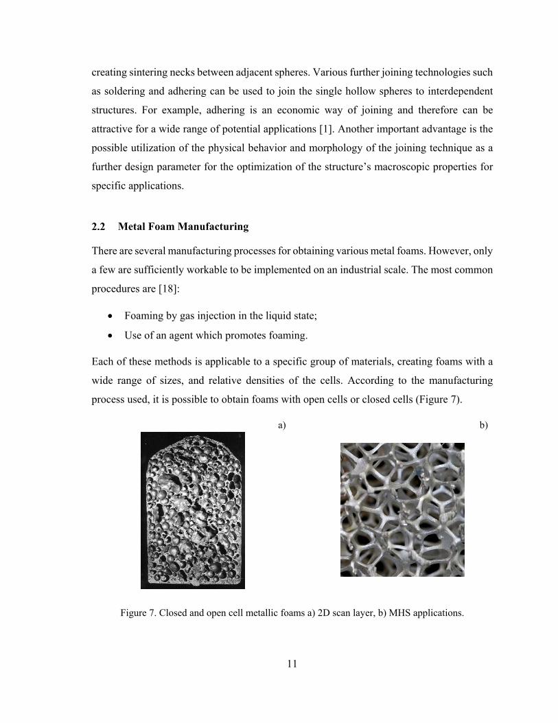
process used, it is possible to obtain foams with open cells or closed cells (Figure 7).
a)
b)
Figure 7. Closed and open cell metallic foams a) 2D scan layer, b) MHS applications.

12
2.2.1 Foaming by Gas Injection
Figure 8 shows the process used in the manufacture of foams by the CYMAT Company
(Canada), and allows to obtain blocks with dimensions up to 2.44 x 1.22 x 0.42 meters and
cells between 5 and 20 mm. This process is unique for aluminium foams, and was originally
developed and patented by Alcan.
The creation of metallic foams using pure metals is not easy, since the resulting foam is not
sufficiently stable and collapses before the metal solidifies. Therefore, silicon carbide,
aluminium oxide or magnesium oxide particles are used to enhance the viscosity of the melt.
Then the melted metal composite is foamed in a second step by injecting gases (air, nitrogen,
argon) into it using specially designed rotating impellers or vibrating nozzles. The function
of the impellers or nozzles is to create very fine gas bubbles in the melted metal and distribute
them uniformly. The bubbles tend to move to the surface where the foam start to dry out
[19]. Finally, it can be pulled off the liquid surface, with a conveyor belt, and is then allowed
to cool down and solidify.
Figure 8. Direct gas injection in the melted metal [19].
The resulting foam characteristics are controlled by injection of air, temperature, cooling
rate and viscosity of the metal. Advantages of the direct foaming process include the large
volume of foam which can be continuously produced and the low densities which can be
achieved. Therefore, this process allows to obtain a metallic foam which is probably less
expensive when compared to other cellular metallic materials.

13
2.2.2 Foaming with Blowing Agents
This process is identical to the first, except it is not a gas blown through the liquid metal. In
this case, a blowing agent is used, that decomposes under the influence of heat and releases
gas which then propels the foaming process. Blowing agents, such as the TiH2, which, when
heated, decomposes into H2 and Ti, releasing gas into the liquid metal are used (Figure 9).
While the metal is in liquid form, calcium is added to increase viscosity. Then TiH2 is added
using particles with small diameters, which are mixed in the metal. Due to release of the
formed gas bubbles, the foam is obtained.
This process is controlled by the amount of agent used, the cooling conditions and the
external pressure. It is possible, using this procedure, to obtain closed-cell foams, since the
viscosity is high enough to prevent the union of several bubbles. The resulting foam has cells
of 0.5 to 5 mm and a relative density of 0.2 to 0.07. Currently, this process is only used to
obtain aluminium foams, since the foaming agent decomposes too rapidly at the high
temperatures used to melt other metals [12], [18].
This technique was developed by Shinko Wire which is the operator of this process, the
commercial name of the product is “Alporas”, which is exactly the porous structure that
forms the core of the panels used in this study [20].
Figure 9. Direct foaming of melts using a blowing agent [21].
1.5% Ca Pure Aluminium
1.6% TiH2
680 co / Thickening 680 co / Foaming Cooling Foamed Block Slicing

14
2.2.3 Investment Casting
In this process, open-cell foams, based on a polymeric material are used as the mold for the
desired metal foam. Such foams have been sold by ERG in Oakland (USA). Where, foams
can be manufactured from molten metal without directly foaming the metal. This is shown
in the schematic Figure 10. According to this process, a polymer foam, e.g. polyurethane
foam, is used as a starting point. If the polymer foam has closed pores, it has to be
transformed into an open porous one by a reticulation treatment. The resulting polymer foam
with open cells is then filled with a slurry of sufficiently heat resistant material, e.g. a mixture
of mullite, phenolic resin and calcium carbonate [22] or simple plaster [23]. After curing,
the polymer foam is removed using a thermal treatment and molten metal is cast into the
resulting open voids which replicate the original polymer foam structure.
Figure 10. Production of cellular metals by investment casting.
To fill the narrow cavities it may be necessary to pressurize and heat the mould, when simple
gravity casting is not sufficient. Difficulties in this process include achieving a complete
filling of the filaments, controlling the usually directional solidification and removing the
mould material without damaging the fine structure too much. Additionally, ERG material
have been reported to be expensive.
2.2.4 Powder Compaction Melting Technique
The method is not restricted to aluminum and its alloys; tin, zinc, brass, lead, gold, and some
other metals and alloys can also be foamed with appropriate blowing agents and process
parameters. Foamed metals can be prepared from metal powders, developed at the
Polymer Foam
Infiltrate with
Slurry and Dry
Remove Polymer
Infiltrate with Metal
Remove Mold
Polymer Filler Metal

15
Fraunhofer-Institute in Bremen (Germany) [23], [24]. The production process begins with
the mixing of elementary metal powders, alloy powders, or metal powder blends with a
blowing agent, after which the mix is compacted to yield a dense, semi-finished product,
Figure 11.
The compaction can be achieved using any technique in which the blowing agent is
embedded into the metal matrix without any notable residual open porosity. Examples of
such compaction methods are uniaxial or isostatic compression, rod extrusion, or powder
rolling.
The precursor has to be manufactured very
carefully because residual porosity or other
defects will lead to poor results in further
processing. The next step is heat treatment
at temperatures near the melting point of
the matrix material. The blowing agent,
which is homogeneously distributed within
the dense metallic matrix, decomposes and
the released gas forces the melting
precursor material to expand, forming its
highly porous structure. The time needed
for full expansion depends on the
temperature and size of the precursor and
ranges from a few seconds to several
minutes.
Figure 11. Powder compact melting process [24].

16
Applications
Metal foams have properties which make them suitable for automotive industry which has
been extremely interested in them since they were first developed. Potential applications also
exist in ship building, aerospace industry and civil engineering.
Figure 11 a), shows a deformed foam-filled tube. Studies done by FIAT and the Norwegian
University of Science and Technology show that, along with the improved axial energy
absorption, there is also great improvement of energy absorption in off-axis collisions.
Figure 11 b) where foams of two different densities are used to fine-tune the deformation
curve of the absorber [25].
a)
b)
Figure 11. a) Prototypes of Cymat aluminium foam crash absorbers. b) Design example based on
Metcomb aluminium foams of two different densities [25].
In the field of aeronautics and aerospace, one of the most significant examples is a supporting
structure for a rocket in which various properties of these materials are exploit. In this case,
the foam has a structural function, supporting the fuel and contributing to mitigating
vibrations and simultaneously improving the conduction of the heat generated by the
combustion, Figure 12.

17
Figure 12. Applications in aeronautics and aero-space.
In Figure 13 an Alporas aluminium foam core was processed to a composite part in which
the foam is completely embedded in a dense skin. Sand casting was used for the
manufacturing. The skin is made from a AlZn10Si8Mg alloy, whereas the foam core consists
of the typical AlCa1.5Ti1.5 alloy used by Shiko Wire Co. for foaming. The part is designed
such that vibration frequencies up to 370 Hz are damped by the internal friction and/or
interfacial slip between core and skin. Seven hundred machines have been equipped with
this composite part up to now. Noise damping levels up to 60% in the frequency range
mentioned have been achieved.
In another example for such applications, LKR (Austria) and the German car maker BMW
have jointly designed an engine mounting bracket using aluminum foams cores, Figure 14.
It can be loaded with the high weight of a car engine and absorbs mechanical vibrations by
internal dissipation into thermal energy. Stiffness is enhanced and, as the fracture toughness
Figure 13. Transverse beam of a machine. Two insets show cross sections in different direction
of the beam [25].

18
of such composites is high, these parts also increase safety in crash situations. Costs for the
part are only marginally higher than costs for the traditional beam cast with a sand core.
Therefore, the future looks bright for this type of application.
Figure 14. Prototype of a BMW engine mounting bracket manufactured by LKR Ranshofen.
Fromleft: empty casting [25].

19
Chapter 3
Mechanical Characteristics of Metallic Foams
There are a lot of different applications for foams. Examples of applications include
absorbing energy during impact events, lightweight structures and thermal insulation. To use
foams efficiently a detailed understanding of their mechanical behavior is required. The
mechanical properties of foams are related to their complex microstructure and to the
properties of the material of which the cell walls are made. Foams could be visually classified
into two groups: open-cell or closed-cell. However, on the market there are different brands
of foams such as Cymat, Mepura (Alulight) and Shinko (Alporas) obtained by different
manufacturing processes. As is visible in Figure 15, different brands of products have
different structures, sizes of cells, wall thickness, structure uniformity [12]. Therefore, this
section is dedicated to illustrate the general mechanical characteristics of the mettalic foams.
The study of the mechanical behavior of metallic foams properties is quite complex. As
stated previously, the mechanical properties of foams depend not only on the basic properties
of the metallic material constituting the cells, but also depend on the spatial arrangement of
the material (density, cell shape, thickness etc.) [7], [12], [21], [26]. The properties of this
type of structure are always a combination of two properties as shown in Figure 16.

20
a)
b)
c)
Figure 15. Foam structure; a) Cymat with a relative density of 0.04; b) Alporas with a relative
density of 0.09; c) Alulight with a relative density 0.25 [12].
Young's Modulus
The Young's modulus E is traditionally defined as the mechanical property that is measured
by the initial inclination of the stress-strain curve. As such, in the case of metal foams, this
property is intrinsically linked to the porous structure and density of it. In the literature there
are several studies relating the Young's modulus to density, Figure 16. This figure shows the
variability of metal foams for different densities bands and how the Young's modulus varies
for different metallic porous structures [12].

21
Figure 16. Variability of the properties of metal foams, Density vsYoung's modulus [12].
Foam Density
One of the most relevant structural features of foams is its relative density ( s ). It is one
of the most important properties associated for foams structures. The relative density is
defined as the ratio between the effective density of the foam and the density of base solid
material s constituting the cell structure. The fraction of porosity is given by 1 s . This
property is one of the properties that is of great importance to be able to condition the use of
a metal foam in a given application, at the expense of other materials already used [7].
Foam Size Effect
In porous materials, the mechanical properties are dependent of sample size. Therefore,
sample size considerations are important. Where, strength and rigidity depends significantly
on the relationship between cell size and sample size, the surface state and the way the
surfaces are connected or loaded during the tests also affect the obtained results. In case of
simple shear, uniaxial compression and pure bending tests on discrete samples with regular
and irregular microstructures, it was found that the macroscopic (uniaxial) compressive and
bending stiffness decreased with decreasing sample size. The damaged surface of a foam
breaks the existing bonds between cells. In other word, any damage presence in a material
foam at the surface weakens the rest of the foam.

22
In other hand, the opposite effect was also found. Where, the decreasing of the material
sample increase shear stiffness. This effect can be explained by attaching a surfaces to
another moving surface. The fixing of the foam using an adhesive corresponds to the
constraining of the surfaces. This type of fixation results in a stiffer material in an inverse
proportion with the sample size. The smaller the sample, the greater the contribution of this
rigidity in the overall behavior zone [27].
Uniaxial Compression Behavior
The typical result of a uniaxial compression test is shown in the Figure 17. This curve can
be seen in the characteristic spectrum of uniaxial compression cellular materials, and three
different phases can be distinguished:
Figure 17. Typical compression stress-strain curve for metal foams [12].
I. Initially, deformation occur elastically and presents an almost linear development of
stresses with strains. The foam deformation mechanism depends slightly on the
topology of the cells. For low density, open cell foams, this elastic deformation is
mainly due to flexural cell unions. As the density increases, the extent of contribution
of cellular or compression couplings becomes increasingly significant, Figure 18 a),
b) and c). In the case of closed-cell materials, in the union of cells, the cell walls are
tensioned or compressed, increasing the stiffness of the material, Figure 18 d), e). In
the case where there is no breakage of cell walls, the compression of the air trapped
inside also contributes to an increase in the stiffness, which is a more obvious effect
on polymeric materials, Figure 18 f). The compressive strength of a foam
0 Strain,
Plateau
E
Str
ess,
D
I III
II

23
corresponds to the initial peak value, when it exists. It can also be obtained as the
interception of the two pseudo-lines (corresponding to the initial load and
corresponding to the breakdown stress of the material “plateau stress”).
Figure 18. Compressive deformation mechanisms, open cell a), b) and c) / closed cell d), e), f)
[12], [18], [28].
II. The second phase is characterized by a practically constant stress level. This zone
corresponds to the collapse of the cells. The collapse mechanism depends on the foam
base material and can be a fragile or plastic collapse. The cell collapse occurs when
the stresses exceeds a certain value and is in a plane perpendicular to the direction of
loading. The collapsed area will be propagated through the material as the
deformation increases. Plastic collapse in elastoplastic foams results in an almost
(d) (f)(e)
(a) (c)(b)

24
horizontal development in the stress-strain curve. This is a key feature of cellular
materials, which is utilized in the case of energy absorption.
III. The last stage of the compression test curve is related to densification of the material.
As the deformation increases, the cell walls are close and come into contact, which
leads to a rapid increase in the stress-strain curve. The friction between the loading
plate and the surface of the foam causes localized deformation and therefore lower
compressive strength values. As such a lubricant or a surface with a low friction
coefficient should be used [12].
Uniaxial Traction Behavior
The typical result of a uniaxial traction test is shown in the Figure 19.
Figure 19. Typical traction stress-strain curve for metal foams [12].
The stress strain traction curve is initially linear elastic due to the flexibility of the cell wall
mechanism, which is equal to that seen in compression. As a ductile material, the
deformation increases, the cell walls suffer deformation in order to align with the direction
of the stress. These deformations cause an increase in the stiffness of the foam until the
moment when failure occurs. For foams, the stress-strain curve usually shows a brittle
failure, which does not show any plastic deformation. The strain at yield is usually low, 0.2
to 2%.
Elasticity zone
Alignment cell wall
Plastic yield
Str
ess,
Strain, 0

25
Figure 20. Tensile deformation mechanisms, open cell a), b) and c) closed-cell d), e) [12], [18],
[28].
When either in tension or compression, the stress-strain curves foams have an area that can
be considered linear elastic wherein the stress evolve linearly with strain. The stresses on
both cases are usually similar.
In an attempt to determine mathematical expressions relating the elastic properties of the
material with the foam parameters (relative density, Young's modulus of the dense material,
the geometry of the cells, etc.) several different approaches have been used for that problem.
The simplest approach was proposed by Gibson and Ashby [7]. The simple modeling of
Gibson and Ashby can be considered a very simplified consideration of the foam structure,
by reducing and neglecting certain parameters of the foam, which allows an easy
understanding of the deformation mechanisms involved.
(d) (e)
(a) (c) (b)

26
Figure 21. Modelling for the open cells - Ashby and Gibson [7].
For the open cells, Figure 21, the relations were obtained by Gibson and Ashby by shaping
the foam as a set of cubical cells, each consisting of twelve "beams" with T-section and
length L. The adjacent cells are positioned so that the "beams" are found at mid-span. The
behavior of the foam is then obtained by the basic laws of the classical mechanics of beams.
Indeed, the geometries of foams are much more complex than that suggested. However, the
way the material behaves is governed by the same principles. The relationship with the
geometry is established by means of a constant.
For the closed type cells of the Figure 22, analysis is more complicated. When they are
obtained from liquid, as often happens, the surface tension on the faces of the cells can cause
the material to concentrante on the cell joints, resulting in closed cells but with very thin
walls. As a result, the behavior is quite similar to the open cell foams, since the stiffness
contribution of the cell walls is low. However, this is not always the case. There are cases in
which the cell walls have a considerable thickness and such models for calculating the foam
parameters differ slightly from those used previously for open cell foams.

27
Figure 22. Modeling for closed cell / compression, Ashby and Gibson [7].
Metallic Foams Anisotropy
Many of the cellular structures naturally exhibit anisotropy. In naturally occurring structures,
the anisotropy is mainly driven by improved properties in a certain preferred direction. In
the case of foams, the anisotropy is often an undesired result of the manufacturing process
used. For example, in the case of foams produced with blowing air or with the use of an
agent which releases gas, the resulting cells tend to have an elongated shape in one direction
(direction of the gravitational force during the manufacturing process), thus presenting some
anisotropy.
The anisotropy of the cellular material is the result of two different causes: anisotropy and
anisotropy of the cellular structure of the material of the cell walls. In the case of metal foam,
the anisotropy of the material is negligible, resulting in only the effects of the structure [18].
Energy Absorption Properties of Metallic Foams
One of the main characteristics of metallic foams is their energy absorption capability while
deforming. The capacity of energy absorption is measured by the efficiency ratio that
compares the energy absorbed during deformation by a real material with an ideal energy
absorber. An ideal absorber is represented by the rectangular compression curve visible in
Figure 23, which directly presents a maximum allowable deformation while the stress
remains constant throughout the deformation process. The efficiency is defined as the ratio

28
between the energy absorbed during the compression deformation and the energy absorbed
by the ideal absorber:
0
max
s
ef
F s ds
F s s
(3.1)
where maxF s is the highest force that occurs above the deformation s .
Figure 23. Schematic drawing representation a real absorber vs. ideal absorber [7].
Metallic foams, like most of the materials, has a compressive stress variation, which makes
the efficiency also to vary the along deformation. The quality of the energy absorbing system
is defined by the energy retention capacity without affecting the densification zone, from
which the material tends to behave as a homogeneous solid material.
The energy absorbed by the material volume unit corresponds directly to the area under the
stress-strain curve and again the amount of energy absorbed varies with the foam density,
cell morphology, foam base material as well as all the parameters which influence the length
of the visible level in the compression curve of these materials, Figure 24. The absorption of
energy in this type of materials is explained by the irreversible conversion into plastic
deformation energy, which is the explanation for the good capacity for energy absorption by
the foams [29]–[31].
Str
ess,
I
Real
Ideal
Strain,

29
Figure 24. Foam compression curves for different foam densities [32].
Modeling the Foam Elastoplastic Behavior
To describe the elastoplastic behavior of the metal foam core sandwich structure, a specific
model has been used for this type of material, namely, the Deshpande constitutive model
[15]. The justification for this choice is based on:
First, the fact that this constitutive model is capable of describing a mechanical behavior of
porous metallic materials, which are completely different from the solid metallic materials.
This model was developed specifically to treat metal foams. The yield surface was developed
through the correlation of experimental data obtained in a multi-axial test. This test consists
in gradual and simultaneous application of hydrostatic pressure and a uniaxial load. Thus, it
is possible to obtain a set of points in the pressure plane, P, versus equivalent stress, q,
corresponding to the beginning of yielding.
Second, the fact that one of the parameters of the yield surface of the constitutive model, and
consequently the flow rule is the plastic Poisson's ratio. This model cannot correctly predict
the foam behavior that have plastic Poisson's ratios close to zero. Thus, it is expected that
the introduction of this parameter as a variable of the yield surface and the flow rule allows
to make this model applicable to a wider range of foams with various Poisson coefficients
[14], [29], [33].
30
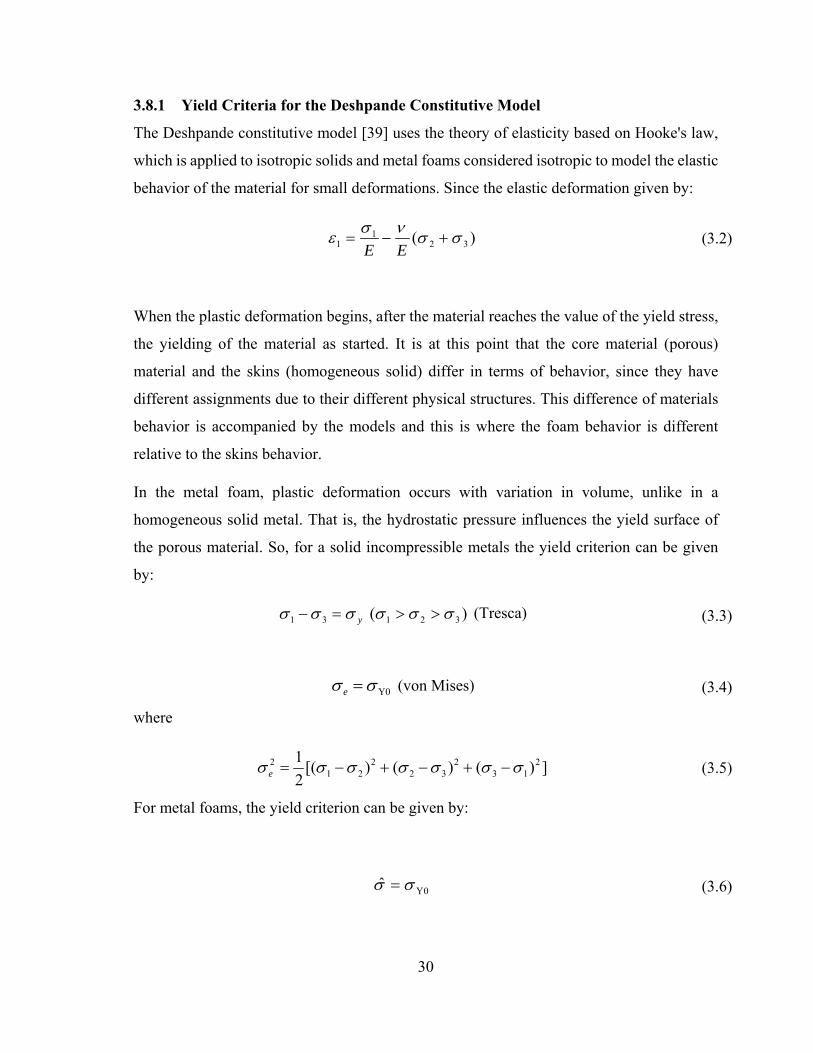
3.8.1 Yield Criteria for the Deshpande Constitutive Model
The Deshpande constitutive model [39] uses the theory of elasticity based on Hooke's law,
which is applied to isotropic solids and metal foams considered isotropic to model the elastic
behavior of the material for small deformations. Since the elastic deformation given by:
11 2 3( )
E E
(3.2)
When the plastic deformation begins, after the material reaches the value of the yield stress,
the yielding of the material as started. It is at this point that the core material (porous)
material and the skins (homogeneous solid) differ in terms of behavior, since they have
different assignments due to their different physical structures. This difference of materials
behavior is accompanied by the models and this is where the foam behavior is different
relative to the skins behavior.
In the metal foam, plastic deformation occurs with variation in volume, unlike in a
homogeneous solid metal. That is, the hydrostatic pressure influences the yield surface of
the porous material. So, for a solid incompressible metals the yield criterion can be given
by:
1 3 1 2 3( )y (Tresca) (3.3)
Y0e (von Mises) (3.4)
where
2 2 2 21 2 2 3 3 1
1[( ) ( ) ( ) ]
2e (3.5)
For metal foams, the yield criterion can be given by:
Y0̂ (3.6)

31
2 2 2 22
1ˆ [( ]
(1 ( / 3) ) e m
(3.7)
where
1 2 3
1( )
3m (3.8)
The stress ̂ is the equivalent stress and e is the von Mises stress, m is the hydrostatic
pressure and is defined as 1
3m kk , it is a parameter that defines the shape of the yield
surface and Y0 the yield stress of the material.
3.8.2 Experimental Definition of the Yield Surface for the Deshpande Constitutive Model
The yield surface of the Deshpande model [15] was developed by the correlation of
experimental data obtained in a multiaxial test. This test consists of progressive and
simultaneous application of hydrostatic pressure and a uniaxial load, Figure 25.
Figure 25. Definition of the yield surface for the Deshpande model [15].
The result of the set of points obtained by Deshpande [15] for the definition of this model,
for different foams and different densities is given in Figure 26.
p
p
p
p
1
3
2
P+
P+

32
Figure 26. Initial yield surfaces of the low and high density Alporas, and Duocel foams. The
stresses have been normalized by the uniaxial yield stress [15].
Based on the experimental results, the experimental definition of the yield surface can be
defined in Figure 27, using a p, q referential, as:
Figure 27. Yield surface for the Deshpande constitutive model in the referential p, q [15], [34].
Y0 0 (3.9)
2 2 2
Y02Φ 0
13
q p
(3.10)
The plastic flux is assumed to be normal to the yield surface, and can be defined by
p N (3.11)
e
m

33
The plastic Poisson ratio can also be written explicitly in terms of the yield surface ellipticity,
where the aspect ratio of the ellipse , based on the expression of the associative plastic
strain (3.11), as:
2
2
1( )
2 3
1 ( )3
p
(3.12)
solving the previous equation, the yield surface due to the plastic Poisson's ratio can be set.
2 (1 2 )9
2 (1 )p
p
(3.13)
In the study of the behavior of materials in plastic regime there are two formulations on
which the constitutive relations are based:
‐ The incremental theory admits the influence of the load trajectory and therefore
relates the stress tensor to increments of plastic deformation;
‐ The deformation theory relates the stress tensor with the deformation tensor.
The first formulation (incremental theory) underlies the so-called plastic flow theory, whilst
the second (the total strain theory) supports the theory of plastic deformation. In general, the
state of plastic deformation depends on the load direction, coinciding both theories for the
case where the load is a straight line trajectory. However, the theory of plastic deformation,
while ignoring the influence of the load direction, it is often used because its application
greatly simplifies the solution of problems in plasticity [35].
Based on the incremental theory, load is proportional to stress. Hence, any load increasing
lead to a deformation increment, which can be decomposed into elastic and a plastic
component, thus it is possible to rewrite the tensor of the elastic deformations

34
e p (3.14)
e N (3.15)
The plastic flow rule can be obtained considering that the plastic strain increment derives
from a potential function. When the yield function coincides with the plastic potential, i.e.
the gradient, commonly known by flux vector is normal to the yield surface, Figure 28 [9-
10, 44-45].
Figure 28. Flow forms: a) Associate; B) Not associated [2].
If we consider a referential p , q and Q f
Nσ σ σ
q p
q p
Nσ σ σ
(3.16)
2
2 2 2 2 2 2 2 2
3 3
( )( 9) ( )( 9)
q q p p
q p q p
N
σ σ
(3.17)
2
1
F Q
σ σ
F Q
1
2
F
Qσ
Fσ
Q
0

35
and 3
:2
q S S the von Mises stress, its derivative is a tensorial derivative, given by:
3 3 3: : :
2 2 2 33:
2
q d p
q d
S S SS S σ I
σ σ σ σS S
3 1 3:
2 3 2
q
q q
ΙΙ
S SI I
σ (3.18)
where 1
( )3
p tr σ is the hydrostatic pressure, its derivative is a tensorial derivative given
by:
1 1:
3 3
p I σ I
σ σ (3.19)
The equivalent plastic strain is given by:
2:
3p p p ε ε (3.20)
resulting in
22 2: :
3 3p N N N N (3.21)
The Deshpande model [15] can then be summarized as follows:

36
Elastic law:
:e e D ε
yield surface:
2 2 22
1( ) 0
13
pyq p
Elastic evolution law:
e N

37
Chapter 4
Aluminum Sheets, Manufacturing and Applications
Aluminum is the most widely used non-ferrous metal. Theoretically it is 100% recyclable
without any loss of its natural qualities. Despite the recycled aluminum being known as
secondary aluminum, it maintains the same physical properties as primary aluminum.
Additionally, it is remarkable known as a low density metal and for its ability to resist
corrosion. Accordingly, it was widely investigated in industry applications. In the fourth
chapter, the sandwich skins will be a presented and discussed.
The aluminum alloy used in the skins, can be defined as a homogeneous solid flat structure
with a given thickness. Pure aluminum has a low strength and cannot be used directly in
applications where resistance to deformation and fracture toughness are essential. Therefore,
aluminum is almost always alloyed, which improve its mechanical properties. The
possibility to combine aluminum and others alloying materials have allowed the
development of new alloys, directed to specific uses.
The present work has used an aluminum plate with a thickness of 1 mm, corresponding to
an aluminum alloy from the series 5XXX, with a typical Young's modulus of 70 GPa and
Poisson's ratio of 0.33.

38
Manufacturing Process of Aluminum Sheets
Aluminum alloys are easily obtained by various metallurgical processes and are available in
a wide variety of forms. One of these known shapes is the flat or plate form. This flat form
is obtained by a process called rolling. It can be described as the plastic deformation process
in which the material is forced to pass between two rollers (rolls) that rotate in opposite
directions with the same peripheral speed. Rollers are apart from each other in a value less
than the thickness of the material to be deformed. The propulsion of the material during
rolling is performed by friction forces, Figure 29
Figure 29. Rolling process.
The rolling process gives rise to aluminum sheet characterized by having a preferred
orientation. This is resulting from the rotation and elongation of the grains in the rolling
direction. This preferred orientation of the grains is the basis of the anisotropy phenomenon
present in laminated aluminum sheets [36].
Applications of Aluminum Sheets
The applications of aluminum alloys are increasingly diverse. Usually it could be found in
daily basis as plate or sheet forms. Aluminum sheets are used in heavy-duty applications
such as those found in the aerospace, military and transportation product manufacturing. For
example, it is machined to be used as the skins of jets and spacecraft fuel tanks. It is used as
a storage tanks in many industries, in part because some aluminum alloys become tougher
at supercold temperatures. This property is especially useful in holding cryogenic (very low

39
temperature) materials. Furthermore, sheets are used to manufacture structural sections for
railcars and ships, as well as armor for military vehicles, Figure 30.
a) b)
Figure 30. a) Aluminum Gas Tank. b) Prototype of German high velocity train ICE made of
welded aluminum foam sandwich
While aluminum sheet represent the most widely used form of aluminum. It could be found
in all of the aluminum industry’s major markets. For example, sheets are used to manufacture
cans and packages. In transportation, aluminum sheet is used to manufacture panels for
automobile bodies and tractor trailers. Moreover, for home appliances and cookware, Figure
31.
.
a) b)
Figure 31. a) Audi A8 car body. b) Cans manufacturing application.

40
Aluminum alloys are widely used in the transport industry due to the high ratio
strength/weight. Which could remarkable lower fuel consumption. Besides, the excellent
corrosion resistance gives greater durability to the vehicle and requires less maintenance.
Mechanical Characteristics of the Aluminum Sheet
The aluminum alloy sheet structure is defined as a solid homogeneous structure, uniform,
flat and with a given thickness. Due to the way as the aluminum sheet is obtained, the sheets
are characterized by having a preferential direction [36].
The tensile test, due to the ease of implementation and the reproducibility of the results make
the tensile test one of the most important mechanical tests.
4.3.1 Uniaxial Tensile Properties
The applied force in a solid body promotes deformation of the material in the direction of
the force. In case of tensile forces, the solid body tends to lengthen. For a metal alloy, the
stress-strain curve may take the appearance shown in Figure 32.
Figure 32. Stress-strain aluminum alloy curve [36].
From point 0 to point A, the curve represents the linear deformation behavior, and the
corresponding stress is proportional to strain, were the Hooke's law is applied as a
constitutive law. Beyond the point B, permanent deformation will occur. Which is known as
A
B
P
Elastic Tension Limit
Proportionality limit
0
Strain,
Str
ess,

41
elastic limit stress. The elastic limit is therefore the lowest stress at which permanent
deformation can be measured.
Other metals have however a slightly different curve from Figure 33. In fact, some metals
have a yield stress value followed by a slight drop. Next, there is an increasing strain, but it
is not accompanied by variations in stress. This region is known as a yield plateau.
Subsequently, the stress increases again, being this phenomenon known as work hardening
(strain hardening).
Figure 33. Stress-strain curve of an alloy with yield level [36].
In the most common metals, the portion of curve AB in Figure 32 is very small in general.
Therefore, it is difficult to distinguish between stress and elastic limit stress proportional
limit. Moreover, also the difference between the stress value of the upper limit of yield
strength and the yield plateau, or yield stress, is usually very small, so that only yield stress
is referred. Due to the difficulty in distinguishing all these parameters, it is usually only
referred to yield strength as the stress required to cause a plastic deformation of 0.2%.
In the plastic region, where the stress exceed the yield stress, the plastic strain increment is
accompanied by a stress increment, and it is said that there was a hardening of the material,
Figure 34 [36].
Yield plateau
Upper yield point
Strain,
Str
ess,

42
Figure 34. Stress-strain curve with unloading and loading [36].
Elasto-plastic Constitutive Model
Constitutive models of solids are usually described by a set of differential equations that
are intended to describe the behavior of the material when subjected to some kind of load.
There are essentially two major groups of models, depending on the type of material and
especially the load type: elasto-plastic and elasto-viscoplastic.
The elasto-plastic models consider that the material behavior is independent of time or the
speed of application of force-displacements. This type of model is used to describe static
or quasi-static problems. While, the elasto-viscoplastic models intended to describe
behaviors with dependence on time or transients, such as fluency or high strain rates. The
elasto-plastic behavior is characterized by the initially elastic response of the material and,
after a certain stress value by an essentially plastic behavior, Figure 35 [36].
Strain,
A
OA’
Str
ess,

43
Figure 35. Plastic-elastic behavior – elasto-plastic hardening model [36].
Taking as a starting point the model of Figure 36, which features a one-dimensional
rheological model, where a a force and consequently a stress ( ) are applied, causing a
stretch l , which could be calculated as the following:
0
l
l
(4.1)
Considering the following additive decomposition of the deformation on the elastic and
plastic components:
e p (4.2)
Figure 36. Elastoplastic rheology model [37].
O
E Friction
Strain, S
tres
s,

44
The material behavior, when there is an extension caused by an applied load is elastic to a
certain point, called elastic limit. The Stress at the elastic limit is the yield stress ( Y0 ),
after which the material deform plastically. The linear-elastic behavior is characterized by
the spring constant and is obtained by the expression:
e p E E (4.3)
The plastic deformation starts when the applied stress reaches the value of yield stress (
Y0 ). When the applied stress reaches Y0 , and a comparison is made with the yield stress,
this is called the yield criterion. In Figure 36, the yield stress corresponds to the friction
between the plates. When the yield point is reached, this value may or may not remain
constant while increasing the deformation. If this value does not depend on the increased
plastic deformation it is said that the material has a perfectly plastic behavior. Moreover,
if the value of the yield stress increases accompanied by a plastic deformation growth, it
is said that the material is suffering hardening.
The materials numerically modeled by an elastoplastic formulations are distinguished by
presenting an approximately linear elastic behavior for small deformations. According to
the theory of elasticity for small deformations, the deformation tensor is defined as
follows:
1( )
2s Tu u u (4.4)
, ,
1
2ij i j j iu u (4.5)
where u is the displacement gradient, and us is its symmetrical part.

45
Considering the bar represented in Figure 37, whose central axis coincides with the axis
(1,0,0)X , and on which a reference point is placed (the particle with 1 X coordinate),
with the left end considered as a reference. The left edge is fixed, while on the other end
a normal force is applied. Initially the normal tensile stress causes a longitudinal extent of
the bar, which drives the reference point to a new coordinate of 2 1 1 X X u , so that it
suffered a displacement in the axial direction of 1u . In a second stage a second normal
force is applied, which moves the reference point trough the distance of
3 2 1 2 X X u X u , whereby the material point advanced u in relation to the
previous position.
Figure 37. Law of decomposition [36].
For simplicity of the exposition only those variables (and its derivatives) will be
considered for the coincident axis with the bar axial axis.
Regarding to the first part of the deformation, the deformation gradient, and considering
only its non-zero component:
2 1 1 11,1
1 1 1
1X X u u
FX X X
(4.6)

46
as the same component on the second phase, and considering the initial position, the final
configuration of the first stage, we have:
3 21,1
2 2 2
1X X u u
FX X X
(4.7)
In the final state, if the position of the point 3 X , was achieved with a single increment, the
deformation gradient would be:
31,1
1
XF
X (4.8)
The same result is obtained by multiplying (4.6) through (4.7):
3 321,1 1,1 1,1
1 2 1
X XXF F F
X X X (4.9)
corresponding to the full elongation:
3 1 2
1 1
X X u
X X (4.10)
Considering the rules for small displacements 1u and 2u, when compared to the size 1X, the
extension in each of the phases is the following:
2 1 1
1 1
X X u
X X (4.11)
3 2
1 1
X X u
X X
(4.12)

47
Adding the extensions of each stage results:
3 2 3 12 1 2
1 1 1 1
X X X XX X u
X X X X (4.13)
where the value of the total length was calculated as if the deformation occurred in a single
phase.
The multiplication performed in (4.9) is called a multiplicative law of decomposition, while
the addition made in (4.13) is called the additive law of decomposition. It should be noted
that the calculation of the extension is only valid for small deformations. Hence, in small
deformations it’s possible to use the law of additive decomposition. Whereas for large
deformations it can be advantageous to use the multiplicative law [38], [39].
By matching the first elastic domain phase with the second plastic domain phase, function
of the deformation tensor, and the deformation gradient F :
e pF F F (4.14)
, , ,e p
i j i j j iF = F F (4.15)
e p (4.16)
e pij ij ij (4.17)
Thus, formulations involving small elastoplastic deformations normally decompose the
deformation tensor in an elastic component and a plastic component. Therefore, it is
appropriate to provide mathematical models that reflect the physical phenomena of elasticity
and plasticity, separately.

48
The elastic behavior is described by the theory of elasticity. It now matters to define the
mathematical model for the plastic component of deformation.
4.4.1 Yield Criteria
The appearance of the plastic behavior is conditioned by a yield criterion, which in its most
general form, can be formulated as follows:
, 0F σ α (4.18)
were α indicates a set of hardening variables and σ the stress tensor. For an isotropic
material, wherein the plastic yield depend solely on the magnitude of the principal stresses,
and not its orientation in the space of the stress, the scalar function F becomes dependent
only on a scalar value known as the hardening parameter :
Y( , ) = ( ) - ( ) 0f F σ σ (4.19)
where ( )f is the yield function. This function can take several analytical forms with
different geometric representation in space.
Since in (4.19) we can conclude that if at a point in a deformable material body verifies
Y( ) < ( )f σ , the body at that point will present an elastic behavior. On other hand, if
Y( ) = ( )f σ , the behavior is plastic. After reaching this state, the subsequent behavior of
this material point, shall be determined by the variation of f with respect to ,
T
d df
f
σσ
(4.20)
where f σ is a normal vector to the yield surface of Figure 38, with the components of
and its variation ( d ) arranged in a vector form [36].

49
Figure 38. Orthogonality condition in the stress space 1 2 [36].
‐ If 0df , this indicates that an elastic unloading situation is occurring. The new stress
state is located inside the yield surface, with the material recovering, with an elastic
behavior;
‐ If 0df , this indicates that the stress state has reached the yield point, which
corresponds to a plastic condition, for materials showing a perfectly plastic behavior;
If 0df , indicates that the stress state is maintained on the yield surface, which is
not maintained constant. This is what happens in the behavior of the material shows
hardening.
4.4.2 von Mises Yield Criterion
von Mises suggested that the yield occurs when the second invariant 2J of the deviatory
stresses reached a critical value [38]:
2
1Φ 0
2J (4.21)
where Φ , depends on the hardening parameter and is the radius of the yield surface.
Due to the dependency on 2J , the plasticity theory using this criterion together with the
O

50
associative law is referred in the literature as the 2J flow theory. Geometrically, the von
Mises criterion is shown and compared with the Tresca criterion in Figure 39.
Figure 39. Representation of the Tresca and von Mises yield criteria [37].
For the tensile test, Y
2Φ
3 whereby the effective stress, or so-called von Mises stress
, in terms of the tensor of the deviatory stresses is given by
2
3 33 : :
2 2 ij ijJ S S S S . For this type of material, which will be used for the
aluminum skins, the plastic deformation does not depend on the hydrostatic pressure and the
criterion can be written as follows:
Y Y
3 3( , ) = : - ( ) : - ( )
2 2 ij ij F σ S S S S (4.22)
4.4.3 Hardening Rule
The hardening rule establishes the conditions for a new plastic flow to occur, after the plastic
state of the material is reached. This situation is due to the fact that the yield surface can
continuously change while the plastic flow is occurring.
von Mises
(J2 constant)
Tresca
( constant)

51
In expression (4.18) a set of hardening variables is introduced, contained in a vector, α .
Basically there are two types of approaches for the dependency of any internal hardening
variable i α , (1 )hardningi n [40]:
i. If a hardening variable is assumed to be dependent on the effective plastic strain
( )pi i , then deformation occurs with hardening, wherein the effective plastic
deformation, p is defined as follows [41], [42].
2 2: :
3 3p p p p p
ij ij ε ε ε ε (4.23)
This actual plastic deformation "reflects the history" of the plastic deformation process, and
not simply it’s initial and final state:
1 2
0 0
d 2d d d : d
d 3
pijt p
p p p pij ijt
t
ε ε (4.24)
ii. The second possibility is called energetic hardening and the hardening variable is related
to total plastic work ( )pi i W , [43] in which:
0 0
: d d
p pij ij
p p pij ijW
σ ε ε (4.25)
According to Nayak and Zienkiewicz in the case of materials in which it is possible to apply
the von Mises criterion, the two hardening models described are equivalents, with the curves
obtained in tensile testing leading to the same degree of hardening[43].

52
The evolution of the yield surface can be classified according to three basic models [44]:
If the subsequent yield surface caused by the plastic strain increment is exclusively
a uniform expansion of the previous yield surface, the hardening model is called
isotropic [45]. For the two dimensional case, it is exemplified in Figure 40 a). This
model proposed by Odquist [46] presents the main advantage of its simplicity,
however, it is not capable to reproduce certain real aspects of materials deformation,
such as the Bauschinger effect [47].
If the subsequent yield surface, maintains the same shape, but is simply moved within
the stress space as a rigid body, the type of hardening is said to be kinematic Figure
40 (b) [48], [49]. This hardening mode, appeared with the objective of modelling a
visible phenomenon occurring experimentally, the Bauschinger effect, occurring in
materials subjected to prolonged cyclic loading schemes.
Distortional hardening, in which the expansion, translation and rotation of the yield
surface, or even the shape change are possible [50].
Figure 40. a) Isotropic increment. b) Kinematic increment [35].
In order to mathematically model the first two hardening modes, it is assumed that the choice
of hardening variables in the following vector can be the following:
T ,p b p α σ (4.26)
Yield surface
Initial yield surface
Yield surface
Initial yield surface
a) b)

53
wherein the scalar value of the effective plastic strain is sufficient to define any isotropic
hardening [51].
Equation (4.19) can then be reformulated by adding the kinematic hardening and, assuming
the isotropic hardening, resulting in:
Y( , ) = - 0b p pf F σ α σ σ (4.27)
Based on (4.27), it is important to define the laws for the isotropic hardening and kinematic
hardening. For the isotropic hardening, it can assume a function, depending only on the yield
stress effective plastic strain [32]:
Y0p
Y h (4.28)
expressing the rule for the isotropic hardening as following:
p pYd H d (4.29)
where, H is the derivative of the general function h , in relation to p .
Besides the perfectly plastic behavior, 0h , in practical applications two cases are typically
assumed [51]:
Y 0p
Y H (4.30)
( )Y0 0 1
pnY H H e
(4.31)
wherein, 0, , H H H
and n are material constants.

54
Anisotropy of Aluminum Alloys
Most of the metal alloys have a tensile behavior under a specific load, similar to what was
presented previously. However for the particular case of aluminum alloys in sheet form, the
preferred orientation resulting from the rolling process causes a variability of the mechanical
properties in different directions, with respect to this preferred orientation. This phenomenon
is known as anisotropy, and this phenomenon is commonly present in the mechanical
behavior of aluminum alloys in the form of sheets.
The influence of anisotropy can be quantified by various parameters, one is through the
anisotropy coefficient that characterizes the distribution of deformation when the material is
subjected to uniaxial tension.
The anisotropy coefficient is defined as the ratio of deformation in the transverse direction
to the load direction and the deformation according to the thickness,
Figure 41. To evaluate the anisotropy in the sheet plane, determines the variation in the angle
between the direction of testing and the direction of laminate, Figure 42[52].
Figure 41. Main directions of a tensile specimen for the calculation of the r coefficients.
2
3
r
(4.32)
21
3

55
Figure 42. Reference used for a sheet to define different angles [52].
4.5.1 Hill Criteria
The Hill criteria (1948) [53] is a widely used criterion for the implementation of planar
anisotropy, especially associated with stamping processes. Despite being a criterion
especially used to describe the anisotropic plasticity phenomena in steels, its simplicity and
ease of application to any state of tension, make this a very versatile criterion.
Hill [53] introduced a simple function as an extension of the von Mises criterion, which can
reproduce the behavior of orthotropic materials. Considering the system of coordinate axes
coincident with the orthotropic axes of Figure 43,
Figure 43. Coordinate system - laminated sheet.
the yield function can be expressed by
Lam
inat
ing
dire
ctio
n 3
Transverse direction
Sheet plane

56
2 2 2 2 2 2 222 33 33 11 11 22 23 31 12( ) ( ) ( ) 2 2 2F G H L M N (4.33)
The parameters F, G, H, L, M and N are material constants which can be experimentally
obtained and ii and ij are the tensor components of the Cauchy stress tensor and is the
equivalent stress.
4.5.2 Hill Criteria - Planar Anisotropy
For laminated structures, such as sheets, the analysis of the above equations can be
simplified, since a plane stress condition can be assumed. By matching the direction 1 to the
direction of lamination, the direction 2 with the direction transverse to the lamination
direction and the direction 3 perpendicular to the sheet plane, Figure 43. By setting the
typical plane stress conditions as: 33 0 , 23 0 and 31 0 the equation (4.33) will
become
2 2 2 211 22 11 22 12( ) ( ) 2 2G H F H H N (4.34)
in the case of a specimen tensile test in which its axis lies at the sheet level and making an
angle with the lamination direction. In Figure 42 it is possible to describe, based on equation
(4.34), the evolution of yield strength as a function of the angle (Hill, 1950 [45]):
0 2 2 2 2
1
sin cos 2 4 sin cosF G H N F G H
(4.35)
The stress-strain relations in plastic regime are obtained from the associative plastic law,
assuming that the infinitesimal plastic deformation increment ijd is always perpendicular to
the yield surface, whatever the orientation of infinitesimal tension increment ijd , pointing
outwards from this surface [45]:

57
ijpij
ij
Fd d
(4.36)
This equation, applied to the anisotropic Hill criteria leads to the following stress-strains
relations in the plastic regime:
11 11 22 11 33
22 22 33 22 11
33 33 11 22 33
23 23
13 13
12 12
( ) ( )
( ) ( )
( ) ( )
p
p
p
p
p
p
d d H G
d d F H
d d G F
d d L
d d M
d d N
(4.37)
The anisotropy coefficient of a sheet for a given r , is defined as the ratio between the
perpendicular plastic deformations during the tensile test. For a test sample, with 0º , 0r
is given by:
220
33
p
p
d Hr
d G
(4.38)
in the 90o direction
1190
33
p
p
d Hr
d F
(4.39)
and in the 45o direction:
045 45
90
2 ( ) 1; 1
2( ) 2
rN F G Nr r
F G G r
(4.40)

58
With the completion of tensile tests on specimens with directions 0º , 90º and
45º it is possible to obtain the anisotropy coefficients or Lankford's r -value and also
the plastic deformation rate.
The usage of this criterion in ABAQUS involves obtaining the anisotropic yield coefficients
iiR obtained through Lankford's r -values coefficients.
Considering the Lankford's r -values for planar anisotropy, 11R , 22R and 33R can be
calculated as:
11 1R (4.41)
22
1
1y x
x y
r rR
r r
(4.42)
33
1y x
x y
r rR
r r
(4.43)
12
45
3 1
2 1x y
x y
r rR
r r r
(4.44)
According to the version implemented in ABAQUS [34] and described in the manual, the
yield function of the Hill criterion is given by
2 2 2 2 222 33 33 11 11 22 23 31
212
( ) ( ) ( ) 2 2( )
2
F G H L Mf
N
σ (4.45)

59
The parameters F, G, H, L, M and N are material constants which can be experimentally
obtained. If 211 , 2
22 and 233 represent the yield stress in the respective directions 1, 2 and
3, the constants ,F G and H are calculated by:
20
2 2 2 2 2 222 33 11 22 33 11
1 1 1 1 1 1 1
2 2F
R R R
(4.46)
20
2 2 2 2 2 233 11 22 33 11 22
1 1 1 2 1 1 1
2 2G
R R R
(4.47)
20
2 2 2 2 2 211 22 33 11 22 33
1 1 1 1 1 1 1
2 2H
R R R
(4.48)
,L M and N
20
2 223 23
3 3
2 2L
R
(4.49)
20
2 213 13
3 3
2 2M
R
(4.50)
were 0 is the yield stress, and 11 22 33 12 13 23, , , , , R R R R R R are the anisotropic yield
coefficients and 0 0 3 .
The flow rule can be expressed as:

60
p f dd d
f
ε bσ
(4.51)
By setting f
33 11 11 22
22 33 11 22
22 33 33 11
12
31
23
( ) ( )
( ) ( )
( ) ( )
2
2
2
G H
F H
F G
N
M
L
b (4.52)
4.5.3 Barlat 91 Criteria
The criteria presented above, although being a criterion which leads to good results from the
point of view of planar anisotropy of steels, is a criterion that can be applied to different
materials, unlike the criteria Barlat et al., especially developed to describe the anisotropy of
aluminum alloys.
For this criterion and for a three-dimensional stress state, the yield function Ψ is given by
[54]–[56]
1 2 2 3 3 1 ˆΨ = 2m mm mS S S S S S (4.53)
Where 1, 2,3iS are the principle values of the tensor S . The m exponent is a parameter
associated with the type of alloy structure, which in the case of a cubic structure with
centered faces is equal to 8 [24] and finally ̂ represents the equivalent stress. The linear
transformation to calculate S is given by
:S L σ (4.54)

61
with L being the linear transformation tensor, which for orthotropic materials is defined by
2 3 3 2
3 3 1 1
2 1 1 2
4
5
6
3 3 3 0 0 0
3 3 3 0 0 0
3 3 3 0 0 0
0 0 0 0 0
0 0 0 0 0
0 0 0 0 0
C C C C
C C C C
C C C C
C
C
C
L (4.55)
where the constants 1 2 3 4 5, , , ,C C C C C and 6C are the parameters that describe the
anisotropy. When the parameters 1..6 1iC (isotropic material) and 2m this criterion
reduces to the von Mises criterion. The application of this criteria to thin sheets means that
the only the constants 1 2 3, ,C C C , and 6C are considered as input parameters, and 4 5 1C C
since they are related to shear in the sheet thickness, which is considered isotropic in that
direction.
The yield surface is described by
ˆΨ = 0Y (4.56)
where Y is the yield stress, which initially takes the value of 0Y , and its evolution is given
by the Voce Law [25]. For hardening, the model uses the kinematic hardening model
proposed by Lemaître and Chaboche [57].

62
Chapter 5
Cohesive Behavior
In order to simulate the adhesive layer within the numerical model of the sandwich,
ABAQUS offers a library of cohesive elements. Modelling the adhesive behavior can be
achieved using two methods, cohesive elements and cohesive interactions. In order to
correctly simulate the cohesive behavior and the debonding or delamination processes, it is
necessary to calibrate the different ABAQUS damage parameters.
Damage Initiation Criterion for Cohesive Behavior
The Maximum Nominal Stress Criterion (MAXS) and Quadratic Nominal Stress Criterion
(QUADS) represent two different damage initiation criteria, based on the stresses, defined
by a traction separation law. When the damage initiation criterion is met, the material
response changes in accordance with a chosen damage evolution law [34]. The damage
initiation criterion is a combination of stresses that satisfy a threshold value, which is a
material function. As a normal failure criterion, a value of 1 or higher indicates that the
initiation criterion is met. For both initiation criteria MAXS or QUADS, the damage
initiation criteria represent the maximum permissible value for the nominal stress when the
deformation is purely normal to the interface or the maximum shear stresses, when the
deformation occurs purely in the first or second shear direction.

63
The Maximum Nominal Stress Criterion (MAXS) can be defined by:
max , , 1.n s to o on s t
t t t
t t t
(5.1)
and the Quadratic Nominal Stress Criterion (QUADS):
2 2 2
1.n s to o on s t
t t t
t t t
(5.2)
where nt is the stress normal to the interface and st and tt represent the shear stresses in the
first and the second shear direction and ont , o
st and ott represent respectively the critical
normal and shear stresses for damage initiation.
The Maximum Nominal Stress Criterion is the damage criterion that was considered for the
numerical simulations of the sandwich composite, as damage was assumed to initiate when
the maximum nominal stress ratio reaches a value of 1. If a damage initiation criterion is
used without an associated evolution law, it will only affect the output results. Thus, the
damage criteria are used to evaluate the propensity of the material to undergo damage
without actually modeling the damage process.
Damage Evolution
The damage evolution law defines the material behavior once the corresponding damage
initiation criterion is reached. A scalar damage variable, D, represents the overall damage in
the material and captures the combined effects of all the active mechanisms. The stress
components of the traction-separation model are affected by the damage variable according
to

64
otherwise no damage to compres
(
s
1 )
ive stiffne
,
ss
0
,n n
nn
D t tt
t
(1 ) ,s st D t
(1 )t tt D t
where nt , st and tt are the stress components predicted by the elastic traction-separation
behavior for the current strains without damage [34].
The Damage evaluation law can be represented by (5.3),
(1 )D (5.3)
Prior to the occurrence of damage, D has a value of 0. When the damage initiation criterion
is meet, and upon further loading, D increases according to a damage evolution law. When
the damage variable D = 1 the material point has completely failed and fracture occurs. The
Damage evolution law can be expressed based on energy or displacement. Specifying either
the post damage-initiation effective displacement at failure or the total fracture energy cG as
shown in Figure 44 , where fm is the displacement at failure and the fracture energy cG is
the area defined under the traction separation curve [34]. A linear post damage-initiation
softening response was used on this work.
Since damage evolution may depend on the mode mix, under a combination of normal and
shear deformation across the interface, and in order to describe the damage evolution, it is
useful to introduce an effective displacement, defined as
2 2 2m n s t
(5.4)

65
where m is the effective displacement and the displacement component in the normal
direction n , and s and t shear component in the second and the third direction,
respectively.
In ABAQUS, damage in the traction-separation response for cohesive surfaces is defined
within the same general framework used for cohesive elements. The main difference
between the two approaches is that for cohesive surfaces, damage is specified as part of the
contact interaction properties.
Figure 44. Linear damage evolution.
5.2.1 Tabular Damage Softening
For tabular softening, it is possible to define the evolution of D directly in tabular form. D
must be specified as a function of the effective displacement relative to the effective
displacement at initiation, mode mix, temperature, and/or field variables[34]. However,
specifying the effective displacement as function of mode mix in tabular form considered
optionally, ABAQUS assumes that the damage evolution is mode independent otherwise.
5.2.2 Linear Damage Evolution
Regarding to the work done, linear softening was adopted. In case of damage evolution under
a constant mode mix, temperature, and field variables, ABAQUS uses an evolution of the
damage variable, D, that reduces to the expression proposed by Camanho et. al [58]:
o SeparationBfm
om
Tra
ctio
n
A
cG

66
max
max
( )
( )
f om m m
f om m m
D
(5.5)
where maxm refers to the maximum value of the effective displacement. The assumption of a
constant mode mix at a material point between initiation of damage and final failure is
customary for problems involving monotonic damage.
5.2.3 Damage Convergence Difficulties
Cohesive elements failure are modeled as undergoing progressive damage. The modeling of
progressive damage involves softening in the material response, which is known to lead to
failure. Damage convergence may has difficulties during unstable crack propagation, when
the energy available is higher than the fracture toughness of the material. Viscous
regularization helps in such cases. The possible convergence problem is avoidable using
viscous regularization of the constitutive equations, which causes the tangent stiffness matrix
of the softening material to be positive for sufficiently small time increments[34].
The regularization process involves the use of a viscous stiffness degradation variable, D ,
which is defined by the evolution equation:
1( )D d D
(5.6)
where is the viscosity parameter representing the relaxation time of the viscous system
and d is the degradation variable evaluated in the inviscid backbone model. The damaged
response of the viscous material is given as

67
(1 )t D t (5.7)
5.2.4 Traction Mode Mix
The fracture energy needs to be specified in tabular form of cG versus 1 and 2 , Figure 45.
While, cG needs to be specified as a function of 1 at various fixed values of 2 . Thus, the
relation between cG versus 1 could be represented in Figure 46, where 1 may vary from 0
(purely normal separation) to 1 (purely shear separation).
The corresponding definitions of the mode mix based on traction components are given by
11
2tan
nt
(5.8)
12
2tan t
s
t
t
(5.9)
where 2 2s tt t is a measure of the effective shear traction. The angular measures used
in the above definition (before they are normalized by the factor / 2 are illustrated in Figure 45 [34].
Figure 45. Mode mix measures based on traction[34].
1
2Shear 2
Shear 1
Normal
nt
tt
st

68
Figure 46. Dependence of fracture toughness on mode mix.
The mode-mix ratios defined in terms of energies and tractions can be quite different in
general.. In terms of energies a deformation in the purely normal direction is one for which
0nG and 0s tG G , irrespective of the values of the normal and the shear tractions. In
particular, for a material with coupled traction-separation behavior both the normal and shear
tractions may be non-zero for a deformation in the purely normal direction. For this case the
definition of mode mix based on energies would indicate a purely normal deformation, while
the definition based on tractions would suggest a mix of both normal and shear deformation.
There are two components to the definition of the evolution of damage. The first component
involves specifying either the effective displacement at complete failure fm , relative to the
effective displacement at the initiation of damage om , or the energy dissipated due to failure
CG , Figure 44[34].
Numerical Example
With aid of the ABAQUS library of examples [34], a chosen example was used to illustrate
the theory of the cohesive behavior for two simples cubes which were tied using the interface
cohesive function. Running the given input file, the results are represented below. Where the
Table1 and Table 2 illustrate the damage criteria and the martial properties respectively.
cG
0 1Mode Mix
Normal mode
Shear mode

69
Table 1. Cohesive damage criteria.
Table 2. Given cube mechanical properties.
Given Prop
Young's Modulus E [GPa] 3
Poisson's Ratio 0
a) b)
Figure 47. Problem geometry. a) Un-deformed cubes. b) Deformed cubes after separation [34]
Figure 48 shows the evolution of the force applied at the top cube, presenting a typical
damage behavior, similar to what is shown in Figure 44. After traction loading the top cube
with a displacement of 0.1mm the damage starts to propagate through the cohesive tie, and
the structure loses its integrity.
Elastic Properties Damage Initiation Damage Evolution
E/Enn G1/Ess G2/Ett Nominal
Stress Normal mode
Nominal Stress First Direction
Nominal Stress Second
Direction
Total / Plastic Displacement at Failure
[m]
1E+011 1E+010 1E+010 2.5E+008 2.5E+008 2.5E+008 0.05

70
Figure 48 ABAQUS example, simple cohesive interface, linear damage behavior
Displacement [mm]
0.0 0.1 0.2 0.3 0.4 0.5
For
ce [
N]
0
10000
20000
30000
40000
50000

71
Chapter 6
Numerical Simulations
Within chapter 6, we are going to present the data that the numerical modeling conducted.
The three-points bending test and the unconstrained bending test were simulated using the
finite element method, using ABAQUS software. Due to the symmetry of the problems, only
a quarter of the geometries were modeled, which improves the numerical stability and
reduces the computational time.
The numerical simulations were conducted with and without the inclusion of the adhesive
layer, in order to verify the adhesive influence on the numerical results. The adhesive layer
and corresponding debonding effect was modeled in ABAQUS using two different
approaches, by using a thin (0.05 mm thickness) layer of cohesive elements (between the
foam and the top and bottom skins) and by using a cohesive interface property, between the
foam and aluminum skins. Frictionless contact was assumed in the different contact pairs,
between the skins and tools (assumed as rigid and modeled with rigid surfaces).
In reference [20] more details can be obtained regarding the experimental results for the
foam compression test and aluminum skins tensile tests.

72
Experimental Data
The results below were collected and represented based on previous experimental work [20],
obtained on previous works of the group.
6.1.1 Experimental Data Used for the Aluminum Metal Foam
The current study uses the closed cell foam, ALPORAS, developed in Japan by the Shinko
Wire Company in the 90’s. It is an aluminum alloy AlCa1.5Ti1.5 with a density of 0.25
g/cm3, has a relative density of about 9% and the porous size is 4-6 mm [59]. The
characterization of the aluminum foam (Alporas foam 9% ) was carried out by means of
uniaxial compression tests.
To do this characterization, the dimension of the specimens was defined as being at least
seven times the size of the cells, in order to dissipate the effects of size. Three specimens
with 40x40x50 mm were used in the tests Figure 49 a). The foam specimens were saw from
a thick (50 mm) foam plate, supplied by the aluminum company. The properties of this foam
plate are identical to the foam used in the composite panels. In these tests the force–
displacements values were measured in order to define de characteristic curve of the
material.
a) b)
Figure 49. Aluminum foam compression test. a) Experimental, b) Numerical.
50 mm
40 mm 20 mm
25 mm

73
Figure 50 shows the three curves obtained from this test. The curves show a good agreement
with traditional curves describing the typical behavior of a porous material Figure 17.
Comparing the curves among themselves, one can see that they are very similar, which
allows defining the corresponding characteristic curve.
The curve shown in Figure 50 defines the foam hardening. According to Deshpande [7] in a
closed cell foam with a relative density of 8.4 % the parameter which defines the shape of
the yield surface α is equal to 2.11. For the same type of foam used in this study, with a
relative density about 9 %, α is considered equal to 2.11 and the constants can be calculated
from Equations (3.16) and (3.12):
2
32.11 1.71
9
kk
k
(6.1)
1.71 3(1 2 0.013)p pk (6.2)
a) Experimental curves. b) Tested sample.
Figure 50. Experimental uniaxial compression tests.
Displacement [mm]
0 5 10 15 20 25 30
For
ce [
N]
0
1000
2000
3000
4000
5000
Sample #1Sample #2Sample #3

74
To obtain the stress – strain curves from the force–displacements curves (compression test);
the total area of the section was considered. Although the pores in the foam do not contribute
to the resisting area, they tend to disappear, with the compaction of the material [6], [19],
[60].
Therefore, as a first approximation, the entire section of the specimen can be considered as
its resistant area. With this consideration, and in conjunction with the curves of Figure 50,
one can obtain the stress–strain characteristic curve for the metal foam, Figure 51[61].
Figure 51. Experimental stress-strain curve for the aluminum foam.
6.1.2 Experimental Data Used for the Aluminum Skins
The aluminum skins used in the composites for the present work have 1 mm thickness, and
are composed by an aluminum alloy (AlMg3) EN AW 5754, with a typical Young's modulus
of 70GPa [59].
In order to verify the influence of the rolling direction on the stress-strain behavior of the
aluminum skins, traction tests with skin samples were conducted for 3 different angles in

75
relation to the rolling direction. Figure 52 shows the stress-strain behavior obtained for the
aluminum skins, for samples aligned with the rolling direction (RD 0º), 45º and 90º.
Figure 52. Aluminum sheet experimental stress-strain curve.
Since the results obtained for the different angles in relation to the rolling direction allowed
to obtain similar results, an isotropic behavior was assumed for the skins.
Parameters Used for the Numerical Simulations
The parameters describing the elasto-plastic behavior of the foam are presented in Table 3.
Table 3. Foam mechanical properties
Young's
Modulus
E [GPa]
Poisson's
Ratio
Compression
Yield
Stress Ratio k
Plastic
Poisson's
Ratio p
Elastic 0.354 0.33
Plastic 1.71 0.013
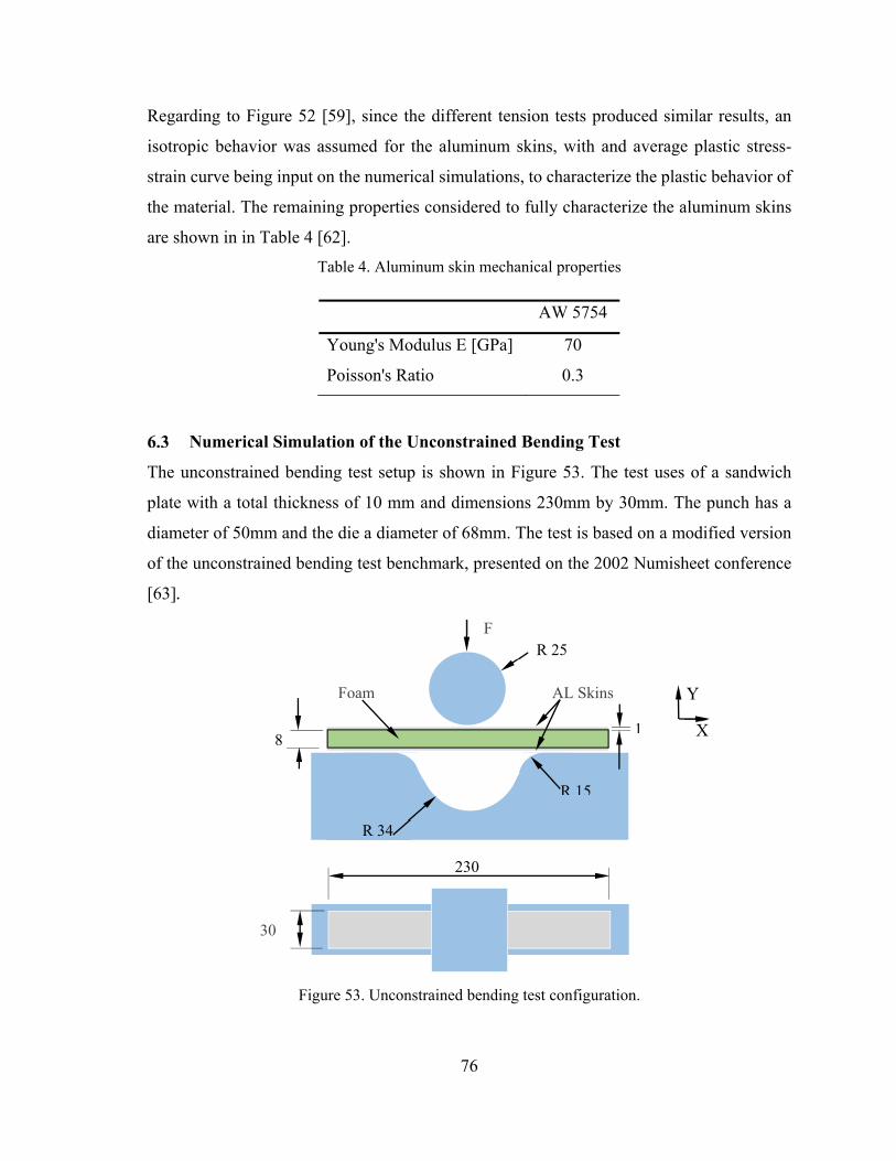
76
Regarding to Figure 52 [59], since the different tension tests produced similar results, an
isotropic behavior was assumed for the aluminum skins, with and average plastic stress-
strain curve being input on the numerical simulations, to characterize the plastic behavior of
the material. The remaining properties considered to fully characterize the aluminum skins
are shown in in Table 4 [62].
Table 4. Aluminum skin mechanical properties
AW 5754
Young's Modulus E [GPa] 70
Poisson's Ratio 0.3
Numerical Simulation of the Unconstrained Bending Test
The unconstrained bending test setup is shown in Figure 53. The test uses of a sandwich
plate with a total thickness of 10 mm and dimensions 230mm by 30mm. The punch has a
diameter of 50mm and the die a diameter of 68mm. The test is based on a modified version
of the unconstrained bending test benchmark, presented on the 2002 Numisheet conference
[63].
Figure 53. Unconstrained bending test configuration.
30
F
AL SkinsFoam
230
R 34
R 15
X
Y
R 25
8 1

77
6.3.1 Unconstrained Bending Test Numerical Model
In the numerical modelling of the three point bending test only 1/4 of the actual specimen
was modelled corresponding, improving the convergence and reducing the computational
time.
The mesh consists of 5160 C3D8R elements for the aluminum skins (eight-nodes,
displacement-based, reduced integration finite element), 8600 C3D8 elements for the foam
and 1720 COH3D8 cohesive elements for the cohesive layers.
For the numerical simulation with the cohesive interaction, the mesh consists of 4800 C3D8I
elements for the aluminum skins and 6400 C3D8 elements for the foam. The overall mesh
can be seen in Figure 54
Figure 54. Finite element mesh for three point bending test.
After specifying the mesh properties and modeling the skin and the foam numerically,
cohesive parameters need to be studied and adjusted. In order to calibrate the cohesive
parameters, in the following sections a comparison will show the effect of each one
individually.
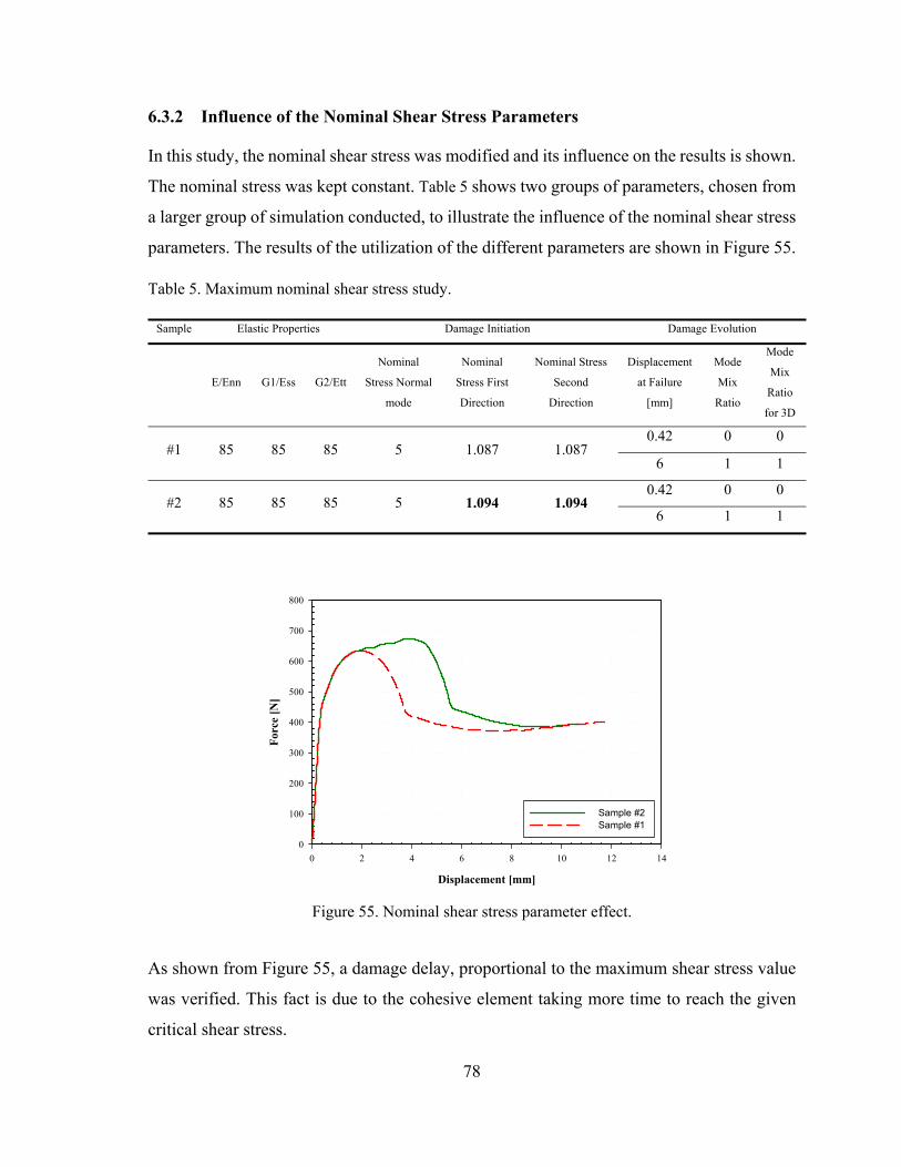
78
6.3.2 Influence of the Nominal Shear Stress Parameters
In this study, the nominal shear stress was modified and its influence on the results is shown.
The nominal stress was kept constant. Table 5 shows two groups of parameters, chosen from
a larger group of simulation conducted, to illustrate the influence of the nominal shear stress
parameters. The results of the utilization of the different parameters are shown in Figure 55.
Table 5. Maximum nominal shear stress study.
Sample Elastic Properties Damage Initiation Damage Evolution
E/Enn G1/Ess G2/Ett
Nominal
Stress Normal
mode
Nominal
Stress First
Direction
Nominal Stress
Second
Direction
Displacement
at Failure
[mm]
Mode
Mix
Ratio
Mode
Mix
Ratio
for 3D
#1 85 85 85 5 1.087 1.087 0.42 0 0
6 1 1
#2 85 85 85 5 1.094 1.094 0.42 0 0
6 1 1
Figure 55. Nominal shear stress parameter effect.
As shown from Figure 55, a damage delay, proportional to the maximum shear stress value
was verified. This fact is due to the cohesive element taking more time to reach the given
critical shear stress.
Displacement [mm]
0 2 4 6 8 10 12 14
For
ce [
N]
0
100
200
300
400
500
600
700
800
Sample #2 Sample #1
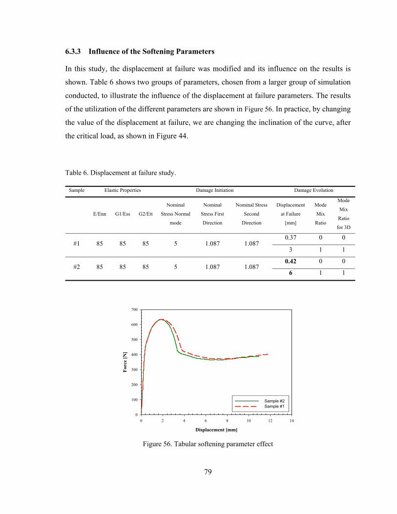
79
6.3.3 Influence of the Softening Parameters
In this study, the displacement at failure was modified and its influence on the results is
shown. Table 6 shows two groups of parameters, chosen from a larger group of simulation
conducted, to illustrate the influence of the displacement at failure parameters. The results
of the utilization of the different parameters are shown in Figure 56. In practice, by changing
the value of the displacement at failure, we are changing the inclination of the curve, after
the critical load, as shown in Figure 44.
Table 6. Displacement at failure study.
Sample Elastic Properties Damage Initiation Damage Evolution
E/Enn G1/Ess G2/Ett
Nominal
Stress Normal
mode
Nominal
Stress First
Direction
Nominal Stress
Second
Direction
Displacement
at Failure
[mm]
Mode
Mix
Ratio
Mode
Mix
Ratio
for 3D
#1 85 85 85 5 1.087 1.087 0.37 0 0
3 1 1
#2 85 85 85 5 1.087 1.087 0.42 0 0
6 1 1
Figure 56. Tabular softening parameter effect
Displacement [mm]
0 2 4 6 8 10 12 14
For
ce [
N]
0
100
200
300
400
500
600
700
Sample #2 Sample #1

80
Figure 56, represent the effect of the displacement at failure parameter effect. By changing
the displacement at failure, the inclination of the softening the change the declination of the
damage. Soften effect would represent the loss in composite sandwich stiffness while
damage propagation.
6.3.4 Influence of the Cohesive Stiffness Parameter
In this study, the stiffness parameters were modified its influence on the results is shown.
Table 7 shows two groups of parameters, chosen from a larger group of simulation
conducted, to illustrate the influence of the stiffness parameters. The results of the utilization
of the different parameters are shown in Figure 57.
Table 7. Cohesive layer stiffness.
Sample Elastic Properties Damage Initiation Damage Evolution
E/Enn G1/Ess G2/Ett
Nominal
Stress Normal
mode
Nominal
Stress First
Direction
Nominal Stress
Second
Direction
Displacement
at Failure
[mm]
Mode
Mix
Ratio
Mode
Mix
Ratio
for 3D
#1 85 85 85 5 1.087 1.087 0.42 0 0
6 1 1
#2 2000 2000 2000 5 1.087 1.087 0.42 0 0
6 1 1
Figure 57. Cohesive stiffness effect
Displacement [mm]
0 2 4 6 8 10 12 14
For
ce [
N]
0
100
200
300
400
500
600
700
Sample #2 Sample #1

81
Figure 57, shows that there are no distinguished effect with the stiffness variation.
Nonetheless, it was noticed that when using a higher stiffness value, the convergence of the
simulation was considerably slower.
Once, each cohesive parameter were understood, the chosen parameter values were selected
and are shown in Table 8. These values represent the best cohesive damage behavior
simulation, which best aproximate the experimental results.
Table 8. Chosen cohesive parameter using the unconstrained bending test.
Elastic Properties Damage Initiation Damage Evolution
E/Enn G1/Ess G2/Ett
Nominal
Stress Normal
mode
Nominal
Stress First
Direction
Nominal Stress
Second
Direction
Displacement
at Failure
[mm]
Mode Mix
Ratio
Mode Mix
Ratio for
3D
85 85 85 5 1.087 1.087 0.37 0 0
3 1 1
Part of the conducted experiments and numerical work is shown in Figure 58 a) and Figure
58 b) respectively.
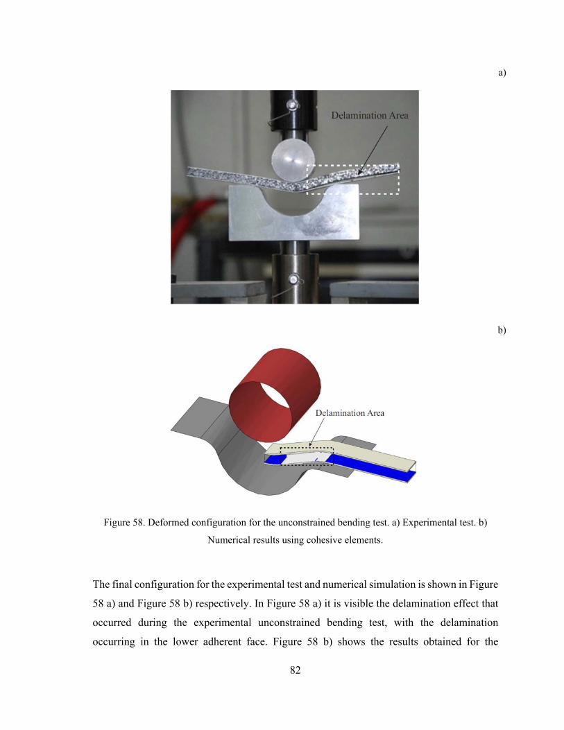
82
a)
b)
Figure 58. Deformed configuration for the unconstrained bending test. a) Experimental test. b)
Numerical results using cohesive elements.
The final configuration for the experimental test and numerical simulation is shown in Figure
58 a) and Figure 58 b) respectively. In Figure 58 a) it is visible the delamination effect that
occurred during the experimental unconstrained bending test, with the delamination
occurring in the lower adherent face. Figure 58 b) shows the results obtained for the

83
numerical simulation, including the cohesive behavior. This numerical simulation was able
to capture the delamination effect, were the delaminated area is represented in white,
corresponding to the deleted elements, while the undamaged cohesive layer is represented
in blue.
Summarizing, the numerical results neglecting the adhesive behavior (no cohesive layer
defined) as well as the inclusion of the adhesive behavior (cohesive element & cohesive face
interaction) are presented in Figure 59.
Figure 59. Unconstrained bending test, experimental and numerical results.
Figure 59 show the numerical and experimental results for the evolution of the force applied
to the central cylinder versus its vertical displacement. It is visible that both numerical
simulations which included the cohesive behavior were able to capture the delamination
effect, and corresponding drop in the applied load, while the simulation without cohesive
behavior produced erroneous results.
When modelling the cohesive behavior by using an interaction property, the numerical
results were closer to the experimental results. When modeling the cohesive behavior using
Displacement [mm]
0 2 4 6 8 10 12
For
ce [
N]
0
100
200
300
400
500
600
700
800
Experimental ResultsCohesive ElementCohesive InteractionNo Cohesive Layer

84
cohesive elements, the deletion of the element upon damage propagation can lead to
interpenetration of the aluminum skins and foam, which could affect the results.
Numerical Simulation of the Three Point Bending Test
The three point bending test setup is shown in Figure 60. The test uses a sandwich plate with
a total thickness of 10 mm and dimensions 200mm by 30mm. The cylinders used on the
experimental and numerical simulation have a diameter of 10mm.
Figure 60. Three point bending test configuration.
6.4.1 Three Point Bending Test Numerical Model
In the numerical modelling of the three point bending only 1/4 of the actual specimen was
modelled, for a better performance in terms of time and convergence. The simulations were
conducted in the finite element software code ABAQUS using a mesh consisting of 4500
C3D8I elements for the aluminum skins (eight-nodes, displacement-based, incompatible
modes finite element), 7500 C3D8 elements for the foam and 1500 COH3D8 cohesive
elements for the cohesive layers.
For the numerical simulations including the cohesive interaction, the mesh consists of 5280
C3D8I elements for the aluminum skins and 7040 C3D8 elements for the foam. The overall
mesh can be seen in Figure 61.
F
30
R 5
AL Skins
8
Foam
160 1F/2 F/2
Y
X

85
Figure 61. Finite element mesh for three point bending test.
The same parameter used for the unconstrained bending test where used for 3 point bending
test, which are shown in Table 9.
Table 9 Chosen cohesive parameter for the three point bending test.
Elastic Properties Damage Initiation Damage Evolution
E/Enn G1/Ess G2/Ett
Nominal
Stress Normal
mode
Nominal
Stress First
Direction
Nominal Stress
Second
Direction
Displacement
at Failure
[mm]
Mode Mix
Ratio
Mode Mix
Ratio for
3D
85 85 85 5 1.087 1.087 0.37 0 0
3 1 1
Part of the conducted experimental and numerical work is shown in Figure 62 a) and Figure
62 b) respectively.

86
a)
b)
Figure 62. Deformed configuration for the three point bending test. a) Experimental result. b)
Numerical results using cohesive elements.
The numerical results for a mesh without considering the adhesive presence (no cohesive
layer or interaction defined) as well as the results assuming the existence of the cohesive
layer (cohesive element or cohesive face interaction), are presented in Figure 63.

87
Figure 63 Experimental and numerical curves for the three point bending test.
A good agreement was obtained between the numerical simulations and the experimental
results, with the model using the cohesive interface presenting the closest results to the
experimental results. As it is visible in Figure 62 a), no delamination occurred during the
experimental test. The numerical parameters inputted on the model were able to capture this
effect, since the cohesive layer/interface did not reach the damage initiation criterion value.
Since no delamination was verified, numerically or experimentally, the results show in
Figure 63 present a similar behavior, even for the case were no cohesive behavior was
considered.
Discussion
Observing the results show in Figure 63, for the three-point bending, and Figure 59 for the
unconstrained bending test, prior to the occurrence if delamination, it can be concluded that
the mechanical properties of the adhesive have a reduced influence on the behavior of the
composite, mainly due to the reduced adhesive layer thickness. This fact can be verified by
comparing the results of the theoretical behavior where no cohesive layer is defined with the
Displacement [mm]
0 5 10 15 20 25 30 35
For
ce [
N]
0
100
200
300
400
500
600
700
Experimental ResultsCohesive ElementCohesive InteractionNo Cohesive Layer

88
remaining results. Furthermore, during the calibration process of the adhesive properties,
there was no distinguished effect on the results regarding to the stiffness variation.
In the three-point bending test where the cohesive layer is not under critical damage stress,
the results are similar. While in the unconstrained bending test, where the experimental
results show a delamination, the results are completely wrong for the model without
adhesive.
Observing the results for the 3-point bending test and the unconstrained bending test, the
stiffness of the cohesive layer (modeled using cohesive elements or interface) is almost
neglected. That could be illustrated by comparing the results to the theoretical behavior
where no cohesive tie is defined. Furthermore, there are no distinguished effect on the results
regarding to the stiffness variation. Nonetheless, it was noticed that with higher stiffness
values the computation time was much longer (slower convergence).
Due to the cellular shape of the foam, the adhesive properties existing in the literature, cannot
be used directly. A process of calibrating the adhesive properties is needed. When this
process is completed, it is possible to correctly simulate the behavior of this kind of
composites.

89
Chapter 7
Conclusion
In 3 point bending test where the cohesive is not under critical damage stress the results are
similar. While in unconstrained test, where the experimental results show a delamination,
the results totally varied. Therefore, the utilization of correct ABAQUS parameters is needed
to obtain a correct modeling of the delamination effect.
The numerical results obtained using ABAQUS are in good agreement the experimental
results. However, cohesive face interaction shows slightly better results when compared to
the cohesive elements. When using the face interaction to include the delamination effect,
slightly better results can be obtained, due to its consideration of the contact forces between
the near faces once the cohesive element fails, which cannot be done when using an interface
with cohesive elements.
Future Work
Studying the cohesive behavior in a real component, produced in a metal foam sandwich
would be an interesting study. This could allow to observe the influence of the cohesive
interface on a real component. This could also allow to further test the calibrated variables,
to verify if they can be applied to different situations.

90
In the numerical simulation of the sheets, a simplification was made, assuming that the sheets
presented an isotropic behavior. The verification of this simplification, against the usage of
a constitutive model, which takes into consideration the anisotropic behavior of the sheets
would be interesting.
The foam is a complex structure, which was simplified on the current study. An interesting
study would be to obtain the real shape of the foam and conduct the same numerical
simulations. This would allow to use the standard properties for the adhesive, without the
need to calibrate this parameters, and the foam properties would be assumed as isotropic,
using a standard constitutive law.

91
References
[1] A. Öchsner and C. Augustin, Multifunctional Metallic Hollow Sphere Structures.
Berlin, Heidelberg: Springer Berlin Heidelberg, 2009.
[2] M. Kleiner, M. Geiger, and A. Klaus, “Manufacturing of Lightweight Components by
Metal Forming,” CIRP Ann. - Manuf. Technol., vol. 52, no. 2, pp. 521–542, Jan. 2003.
[3] A. G. Evans, J. W. Hutchinsona, and M. F. Ashby, “Multifunctionality of cellular
metal systems,” Prog. Mater. Sci., vol. 43, pp. 171–221, 1999.
[4] J. Baumeister, J. Banhart, and M. Weber, “Aluminium foams for transport industry,”
Mater. Des., vol. 18, no. 4–6, pp. 217–220, Dec. 1997.
[5] V. S. Deshpande and N. A. Fleck, “Isotropic constitutive models for metallic foams,”
J. Mech. Phys. Solids, vol. 48, no. 6–7, pp. 1253–1283, Jun. 2000.
[6] R. E. Miller, “A continuum plasticity model for the constitutive and indentation
behaviour of foamed metals,” Int. J. Mech. Sci., vol. 42, no. 4, pp. 729–754, Apr.
2000.
[7] L. J. Gibson and M. F. Ashby, Cellular Solids - Structure and Properties, 2nd ed.
New York: Cambridge University Press, 1999.
[8] Y. Sugimura, J. Meyer, M. Y. He, H. Bart-Smith, J. Grenstedt, and A. G. Evans, “On
the mechanical performance of closed cell Al alloy foams,” Acta Mater., vol. 45, no.
12, pp. 5245–5259, Dec. 1997.
[9] H. Bart-Smith, A. . Bastawros, D. . Mumm, A. . Evans, D. . Sypeck, and H. N. .
Wadley, “Compressive deformation and yielding mechanisms in cellular Al alloys
determined using X-ray tomography and surface strain mapping,” Acta Mater., vol.
46, no. 10, pp. 3583–3592, Jun. 1998.
[10] A. E. Simone and L. J. Gibson, “The effects of cell face curvature and corrugations
on the stiffness and strength of metallic foams,” Acta Mater., vol. 46, no. 11, pp.
3929–3935, Jul. 1998.

92
[11] J. L. Grenestedt, “Influence of wavy imperfections in cell walls on elastic stiffness of
cellular solids,” J. Mech. Phys. Solids, vol. 46, no. 1, pp. 29–50, Jan. 1998.
[12] M. F. Ashby, A. Evans, N. A. Fleck, L. J. Gibson, J. W. Hutchinson, and H. N. .
Wadley, “Metal Foams: A Design Guide,” Mater. Des., vol. 23, no. 1, p. 119, Feb.
2002.
[13] H. Mata, A. Santos, A. A. Fernandes, R. A. F. Valente, M. P. L. Parente, and R. N.
Jorge, “Analysis of Sandwich Shells with Metallic Foam Cores based on the Uniaxial
Tensile Test,” 2011, vol. 1353, no. 1, pp. 1232–1237.
[14] H. Mata, R. Natal Jorge, A. A. Fernandes, R. A. F. Valente, and M. P. L. Parente,
“FEM Analysis of Sandwich Shells with Metallic Foam Cores,” Key Eng. Mater., vol.
473, pp. 659–666, Mar. 2011.
[15] H. Mata, R. N. Jorge, A. Santos, A. A. Fernandes, R. A. F. Valente, and M. P. L.
Parente, “Modeling of Sandwich Sheets with Metallic Foam,” 2011, vol. 1383, no. 1,
pp. 725–732.
[16] T. J. Lu, F. Xu, and T. Wen, Thermo-Fluid Behaviour of Periodic Cellular Metals.
Springer, 2015.
[17] T. K. Stovall, “Closed Cell Foam Insulation: A Review of Long Term Thermal
Performance Research,” Oak Ridge, TN (United States), Dec. 2012.
[18] I. M. A. Duarte, “Espumas metálicas : processo de fabrico, caracterização e simulação
numérica.” 07-Mar-2005.
[19] J. Banhart, “Manufacture, characterisation and application of cellular metals and
metal foams,” Prog. Mater. Sci., vol. 46, no. 6, pp. 559–632, Jan. 2001.
[20] H. T. C. Mata, “Estudo de Estruturas Sandwich Hidroformadas Constituídas por
Núcleo de Espumas Metálicas,” FEUP - Porto, 2014.
[21] J. Banhart, M. F. Ashby, and N. A. Fleck, “Metal Foams and Porous Metal
Structures,” in MetFoam’99.
[22] Y. Yamada and C. Hayashi, “Casting Science and Technology,” p. 103.
[23] Y. Yamada, K. Shimojima, Y. Sakaguchi, M. Mabuchi, M. Nakamura, T. Asahina, T.

93
Mukai, H. Kanahashi, and K. Higashi, Advanced Engineering Materials, vol. 2, no.
4. WILEY-VCH, 2000.
[24] F.-I. Bremen, “Foaminal - Fraunhofer IFAM,” Product information sheet of
“‘Foaminal,’” 1999. .
[25] B. Raj, S. Ranganathan, and S. L. Mannan, Frontiers in the Design of Materials. CRC
Press, 2007.
[26] J. Banhart, M. F. Ashby, and N. A. Fleck, Cellular Metals and Metal Foaming
Technology. Bremen: Verlag MIT Publ., 2001.
[27] Cihan and Tekoğlu, “Size effects in cellular solids,” University of Groningen, 2007.
[28] J. Banhart, Mechanical properties of metal foams Fraunhofer USA Metal Foam
Symposium. Verlag MIT, Bremen: ASM International, 1998.
[29] R. P. M. das Neves, “Modelação computacional de espumas metálicas : modelação
constitutiva do comportamento mecânico de espumas metálicas.” 13-Feb-2009.
[30] J. Banhart, J. Baumeister, and M. Weber, “Aluminium Foams for Automotive
Applications.”
[31] J. Baumeister, J., “Energy absorption of foamed metals prepared by a powder
metallurgical method,” in PTM ’93. Materials by Powder Technology. Proceedings,
1993.
[32] D. R. J. Owen and E. Hinton, “Finite elements in plasticity: theory and practice,” Civ.
Eng., vol. 190, pp. 4767–4783, 1980.
[33] H. Mata, R. N. Jorge, A. A. Fernandes, and R. A. F. Valente, “Study of sandwich
shells with metallic foam cores,” Int. J. Mater. Form., vol. 3, no. SUPPL. 1, pp. 903–
906, 2010.
[34] ABAQUS, Abaqus Analysis User’s Manual Version 6.11. .
[35] R. Natal Jorge and L. M. J. S. Dinis, “Teoria de plasticidade,” FEUP, Porto, 2005.
[36] J. M. Davies, Lightweight Sandwich Construction. 2001.
[37] H. G. ALLEN, Analysis and Design of Structural Sandwich Panels. Elsevier, 1969.
[38] N. Lopes, “Análise e Caracterização da Degradação de Compósitos Reforçados com

94
Fibra de Juta e Fibra de Vidro em Ambiente Controlado (Temperatura & Humidade),”
Instituto Superior Técnico, Lisboa, 2009.
[39] “Composite Materials Handbook, Vol. 3,” 1997. [Online]. Available:
https://app.knovel.com/web/toc.v/cid:kpMHMILH43. [Accessed: 08-Apr-2016].
[40] P. Carvalho, “Análise do Comportamento Mecânico e Identificação do Tipo de Falha
em Estruturas Sandwich com Núcleos de Cortiça,” Instituto Superior Técnico, 2008.
[41] B. Soares, “Estruturas Sandwich Com Utilização De Núcleos De Cortiça,”
universidade tecnico de lisboa, 2007.
[42] M. Leite, “Estudo Experimental, Analítico e Numérico de Vigas em Construção
Sandwich Reforçada com Aplicações ao Transporte Refrigerado de Bens Perecíveis,”
Instituto Superior Técnico, 2004.
[43] D. Zenkert, The Handbook of Sandwich Construction. United Kingdom: EMAS,
1997.
[44] P. Miguel, “Estudo do Comportamento em Flexão de Vigas Compósitas Sandwich,”
universidade tecnico de lisboa, 2010.
[45] R. Hill, The Mathematical Theory of Plasticity. 1998.
[46] F. K. G. Odquist, Math. Mech., Vol.13 ed. 1933.
[47] G. E. Dieter, Mechanical metallurgy. McGraw-Hill, 1976.
[48] W. Johnson and P. B. Mellor, Plasticity for mechanical engineers. Van Nostrand,
1962.
[49] T. J. Thomas, S. Nair, and V. K. Garg, “A numerical study of plasticity models and
finite element types,” Comput. Struct., vol. 16, no. 5, pp. 669–675, Jan. 1983.
[50] B. Ekmark, “On large strain theories in sheet metal forming,” Luleå University of
Technologyy-LTU, 1983.
[51] M. Schonauer, “Unified numerical analysis of cold and hot metal forming processes.”
University College of Swansea, 1994.
[52] J. M. F. Duarte, “Conformação plástica de chapas metálicas : simulação numérica e
caracterização mecânica.” 24-May-1997.

95
[53] R. Hill, “A Theory of the Yielding and Plastic Flow of Anisotropic Metals,” Proc. R.
Soc. A Math. Phys. Eng. Sci., vol. 193, no. 1033, pp. 281–297, May 1948.
[54] F. Barlat, Y. Maeda, K. Chung, M. Yanagawa, J. C. Brem, Y. Hayashida, D. J. Lege,
K. Matsui, S. J. Murtha, S. Hattori, R. C. Becker, and S. Makosey, “Yield function
development for aluminum alloy sheets,” J. Mech. Phys. Solids, vol. 45, no. 11–12,
pp. 1727–1763, Nov. 1997.
[55] F. Barlat, K. Chung, and O. Richmond, “Strain rate potential for metals and its
application to minimum plastic work path calculations,” Int. J. Plast., vol. 9, no. 1,
pp. 51–63, Jan. 1993.
[56] F. Barlat, D. J. Lege, and J. C. Brem, “A six-component yield function for anisotropic
materials,” Int. J. Plast., vol. 7, no. 7, pp. 693–712, Jan. 1991.
[57] J. Lemaitre and J.-L. Chaboche, Mechanics of Solid Materials. Cambridge University
Press, 1994.
[58] P. P. Camanho and C. G. Davila, “Mixed-Mode Decohesion Finite Elements for the
Simulation of Delamination in Composite Materials. NASA/TM-2002-211737,” Jul.
2002.
[59] “Technical Data Sheet, Gleich Aluminium,” 2010. [Online]. Available:
http://gleich.de/de/produkte. [Accessed: 14-Mar-2016].
[60] T. M. McCormack, R. Miller, O. Kesler, and L. J. Gibson, “Failure of sandwich beams
with metallic foam cores,” Int. J. Solids Struct., vol. 38, no. 28–29, pp. 4901–4920,
Jul. 2001.
[61] H. Mata, A. D. Santos, M. P. L. Parente, R. A. F. Valente, A. A. Fernandes, and R. N.
Jorge, “Study on the forming of sandwich shells with closed-cell foam cores,” Int. J.
Mater. Form., vol. 7, no. 4, pp. 413–424, Jun. 2013.
[62] H. Mata, R. Natal Jorge, A. D. Santos, M. P. L. Parente, R. A. F. Valente, and A. A.
Fernandes, “Numerical Modelling and Experimental Study of Sandwich Shells with
Metal Foam Cores,” Key Eng. Mater., vol. 504–506, pp. 449–454, Feb. 2012.
[63] D. Y. Yang, NUMISHEET 2002: Proceedings of the 5th International Conference
and Workshop on Numerical Simulation of 3D Shell Forming Processes -verification

96
of Simulation with Experiment. 2002.

97
Annex A
Paper accepted for the Journal of Adhesion

For Peer Review O
nly
Aluminum Foam Sandwich with Adhesive Bonding:
Computational Modelling
Journal: The Journal of Adhesion
Manuscript ID GADH-2016-0071.R2
Manuscript Type: Review
Date Submitted by the Author: n/a
Complete List of Authors: Sadek, Seif; Universidade do Porto Faculdade de Engenharia, Areias, Bruno; Universidade do Porto Faculdade de Engenharia Parente, Marco ; Universidade do Porto Faculdade de Engenharia Belinha, Jorge; Universidade do Porto Faculdade de Engenharia Santos, Abel; Universidade do Porto Faculdade de Engenharia Jorge, Renato ; Universidade do Porto Faculdade de Engenharia
Keywords: finite element analysis < Methods of analysis, delamination < Phenomena, cohesion < Phenomena, cohesive damage behavior, automotive < Applications
URL: http://www.tandfonline.com/gadh Email: [email protected]
The Journal of Adhesion

For Peer Review O
nly
1
Aluminum Foam Sandwich with Adhesive Bonding: Computational
Modelling
S.H. Sadeka, B. Areias
b, M.P.L. Parente
b*, J. Belinha
b, A.D. Santos
b, R.M. Natal Jorge
b
aFaculty of Engineering, University of Porto, Rua Dr. Roberto Frias, 4200-465, Porto, Portugal
e-mail: seif.sadek@ fe.up.pt
bLAETA, INEGI, Faculty of Engineering, University of Porto, Rua Dr. Roberto Frias, 4200-465
Porto, Portugal
e-mail: {mparente, jbelinha, abel, rnatal}@fe.up.pt, [email protected]
Abstract:
In this work a numerical approach to numerically simulate the delamination effect occurring in
metal foam composites is presented. It is shown that in order to create reliable numerical models
to simulate general components produced with aluminum metal foam sandwiches, the
delamination effect of the aluminum skins from the metal foam must be considered.
Delamination occurs within the polyurethane adhesive layer, causing the loss of the structural
integrity of the structure.
Foam is not a continuum medium, nevertheless, when simulating foam structures, the foam is
commonly assumed as a continuum, with homogeneous properties. This approach requires the
calibration of the mechanical properties of the polyurethane adhesive layer, in order to
compensate the effect of the foam discontinuous structure.
The finite element method was used to numerically simulate a three-points bending test and a
bench bending test. The cohesive behavior was modelled by using a traction separation law. For
the damage initiation criteria, a maximum stress based criteria was used, while for the damage
evolution, a displacement based damage evolution was adopted. The experimental data was
obtained from the previous works of the group, including a compression test, tension test, three-
points bending test and a bench bending test.
Keywords: Finite element analysis, delamination, cohesion, automotive.-
Page 1 of 41
URL: http://www.tandfonline.com/gadh Email: [email protected]
The Journal of Adhesion
123456789101112131415161718192021222324252627282930313233343536373839404142434445464748495051525354555657585960