alternative investments: return driving actors

1

Alternative investments: return driving actors

Keith Elliott1 and Gianluca Marcato2

School of Real Estate & Planning Henley Business School University of Reading Reading RG6 6UD

[ Current Draft: 25th May 2011 ]

ABSTRACT

In an asset allocation process, correlations are particularly important if one

includes 'alternative investments' such as real estate, commodities and hedge

funds, which have been proclaimed to provide diversifying benefits within the

overall portfolio context. However, by looking at correlations between asset

classes alone some diversification benefits may be over or under-stated. More

recently, finance literature has focused on alternative asset classes to study their

behaviour and to identify the main driving factors. Particularly, these studies have

tried to shed light upon the cyclical behaviour of these ‘new’ assets and their link

with overall economic trends.

This paper represents the first comparative study of several asset classes. We

analyse the common driving factors of fourteen (both traditional and alternative)

assets to provide insights into their likely performance over different economic

environments. Firstly, Principle Component Analysis is used to give a better

statistical understanding of the structure of the data and the number of likely

common factors. Subsequently, a number of different univariate and multivariate

regressions are performed using financial and economic variables identified in the

literature. We find evidence of common macroeconomic and financial factors

1 Email: [email protected], Tel: +44 (0)118 378 8175, Fax: Tel: +44 (0)118 378 8172.

2 Email: [email protected], Tel: +44 (0)118 378 8178, Fax: Tel: +44 (0)118 378 8172.

mailto:[email protected]

mailto:[email protected]

2

driving the returns of certain asset classes, with consequences on the reduced

diversification benefits of such assets during particular phases of the business

cycle.

3

1. Introduction

The aim of this paper is to investigate the relationship between the different asset classes further,

more specifically at whether there are any factors which mutually drive the returns of more than

one asset. This is useful for three main reasons; at a basic level it may help us understand how

an asset class should perform under certain circumstances for example under different

macroeconomic states. Furthermore the techniques can perhaps identify if there are strong

common drivers between the assets and thus if any will have low diversifying power in the

common overall portfolio. Finally if underlying factors are identified it may be possible to

replace certain asset with ones that may have other more favourable characteristics, for example

better liquidity.

At a single asset class level there have been numerous studies that focus on the links between the

asset class and macroeconomic variables; however, there has been very little research that looks

at more than one asset class in these terms simultaneously. Most of the original research was

concentrated on stocks and bonds but more recently more work has been performed on other

asset classes, particularly real estate, although commodities and hedge funds have been studied in

these terms as well.

This study will use several methods to attempt to identify the factors that drive returns across a

number of asset classes. In a broad sense it is perhaps possible to divide factor models of the

returns on assets into three general types: fundamental, statistical and macroeconomic (Connor

1995). As we are interested in the factors that are driving different asset classes over time, the

first type of model, those that use cross sectional asset pricing using fundamental factors, are not

applicable to this work. However; the other two general types of model will be used. Firstly,

principle component analysis will be used in order to identify on a statistical basis the number of

likely driving factors and the degree of their effect. Secondly, regression based methods will be

used to identify if macroeconomic variables that have been previously identified in the literature

are proven to affect real estate returns. Ex post return regressions will indicate whether a

variable will have a statistical significant exposure to macroeconomic factors.

4

2. Principle Component Analysis of the Asset Class Returns3

Firstly principle component analysis was performed on four different sets of asset class data. At

a basic level PCA is a mathematical data reduction technique. It is used to transform the original

data set into a number of principal components. Each of these will account for a degree of the

variation within the original data. One study has already performed PCA on multiple asset class

return proxies in the U.K.; Bond et al. (2007). Here the authors find that six common risk

factors explain 99% of the variation in the returns of the 8 core asset classes.

Firstly, it was applied to all of the 14 assets being investigated in this section. Then it was applied

to the data split into two sub-sets, one comprising of nine sub-assets which may be defined as

being traditional assets and another of five ‘alternative’ assets. Fourthly, the technique was

applied to a set of seven sub-asset classes that only included one sub-asset classes in each broad

asset class category was included. For example only U.K. equities and government bonds were

included rather than all seven equity and fixed income sub-asset classes; this was done order to

check that the assets with more sub-asset classes were not biasing the results.

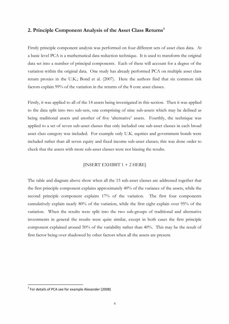
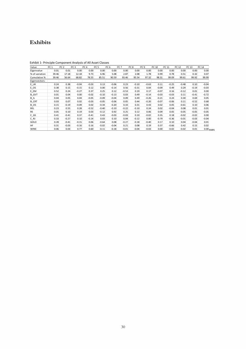
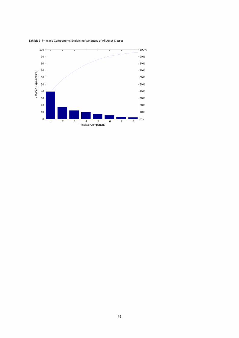
[INSERT EXHIBIT 1 + 2 HERE]

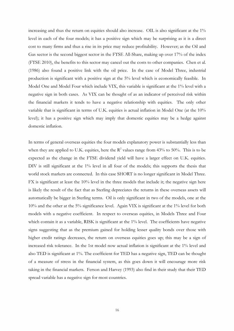
The table and diagram above show when all the 15 sub-asset classes are addressed together that

the first principle component explains approximately 40% of the variance of the assets, while the

second principle component explains 17% of the variation. The first four components

cumulatively explain nearly 80% of the variation, while the first eight explain over 95% of the

variation. When the results were split into the two sub-groups of traditional and alternative

investments in general the results were quite similar, except in both cases the first principle

component explained around 50% of the variability rather than 40%. This may be the result of

first factor being over shadowed by other factors when all the assets are present.

3 For details of PCA see for example Alexander (2008)

5

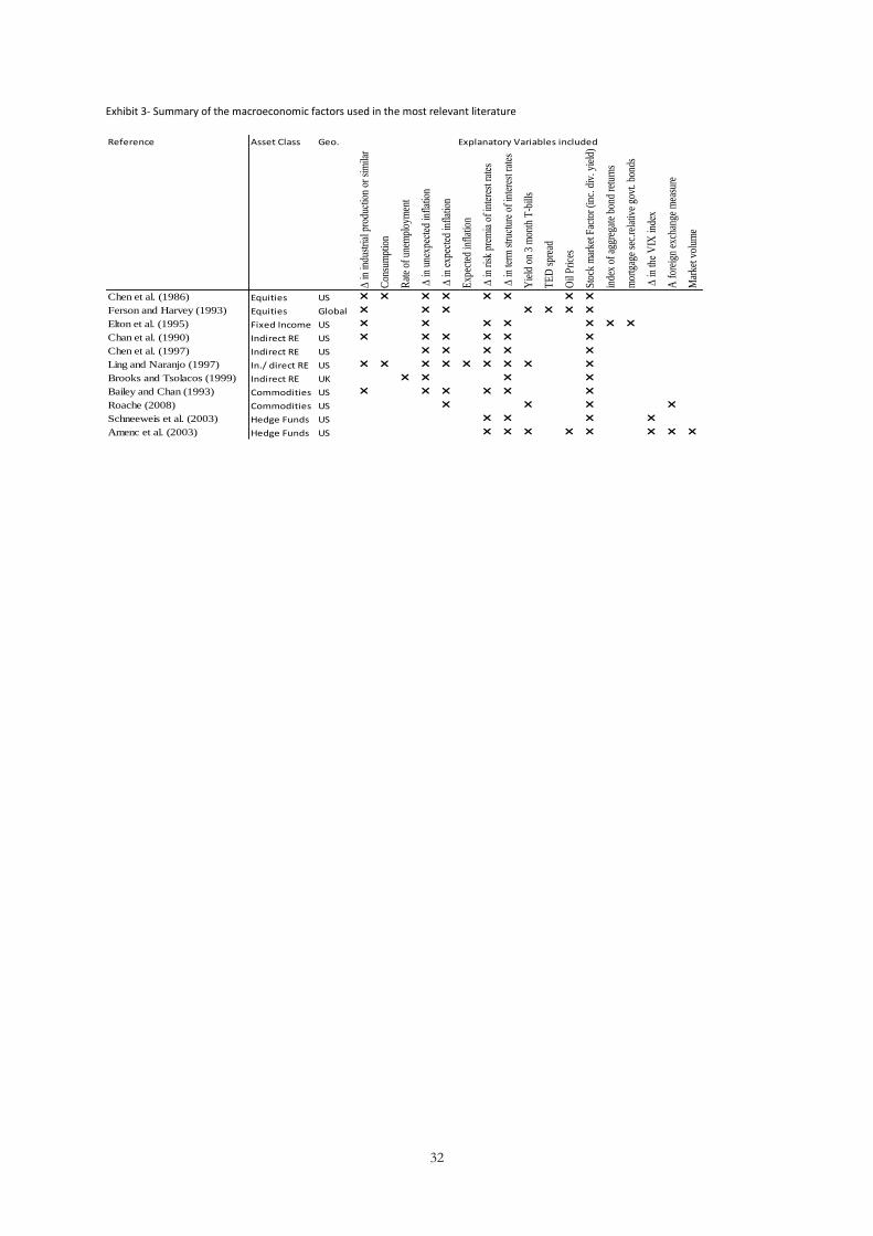
3. Macroeconomic factor models- Background and brief literature review

The purpose of this section is to document the different macroeconomic risk exposures that

different asset classes have. This area of research is related to the Arbitrage Pricing Theory of

Ross (1976) because the factors that are driving asset class returns are also those which can then

be found to be ‘priced in’ to the returns of an individual security. Most of the papers in the area

do come from the pricing point of view but a few concentrate on the macro exposures or study

both. A brief review of the literature in this area is presented below, it documents which assets

are studied; however, it will focus primarily on the macroeconomic variables that the various

authors decided to include in their models.

The first major paper to address, using this framework, that macroeconomic variables may be

connected to asset performance is Chen, Roll and Ross (1986). In this paper the authors explain

the returns of portfolios of equities in the context of several macroeconomic variables and to see

if these risks are priced in. They point out that up to this paper there was a complete ignorance

of the identity of which underlying variables are likely to influence all assets, although there was

theoretical support for their existence. Therefore they state that it is very difficult to determine a

complete list of factors. They use the logic that any factor which changes the discount rate will

be a valid systematic factor. An article which applies a similar methodology to international

equity markets is Ferson and Harvey (1993). The returns of bonds are addressed in a similar

framework to these previous articles by Elton et al. (1995). The first paper to apply this

approach to real estate as an asset class is Chan et al. (1990); Chen, et al. (1997) also look at the

indirect real estate market in the U.S.A. Also addressing real estate are Ling and Naranjo (1997)

and the U.K. based study Brooks and Tsolacos (1999). Bailey and Chan (1993) and Erb and

Harvey (2006) use macroeconomic factors to help explain commodity returns. A paper that

applies a limited multi-factor analysis to hedge fund indices using only a few key macroeconomic

variables is Schneeweis et al. (2003). Secondly in Amenc et al. (2003) use a greater number of

factors to explain the returns of hedge funds. See the table below for a summary of the factors

that were considered by the main papers in this area.

[INSERT EXHIBIT 3 HERE]

.

6

4. Data

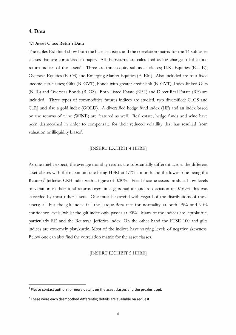
4.1 Asset Class Return Data

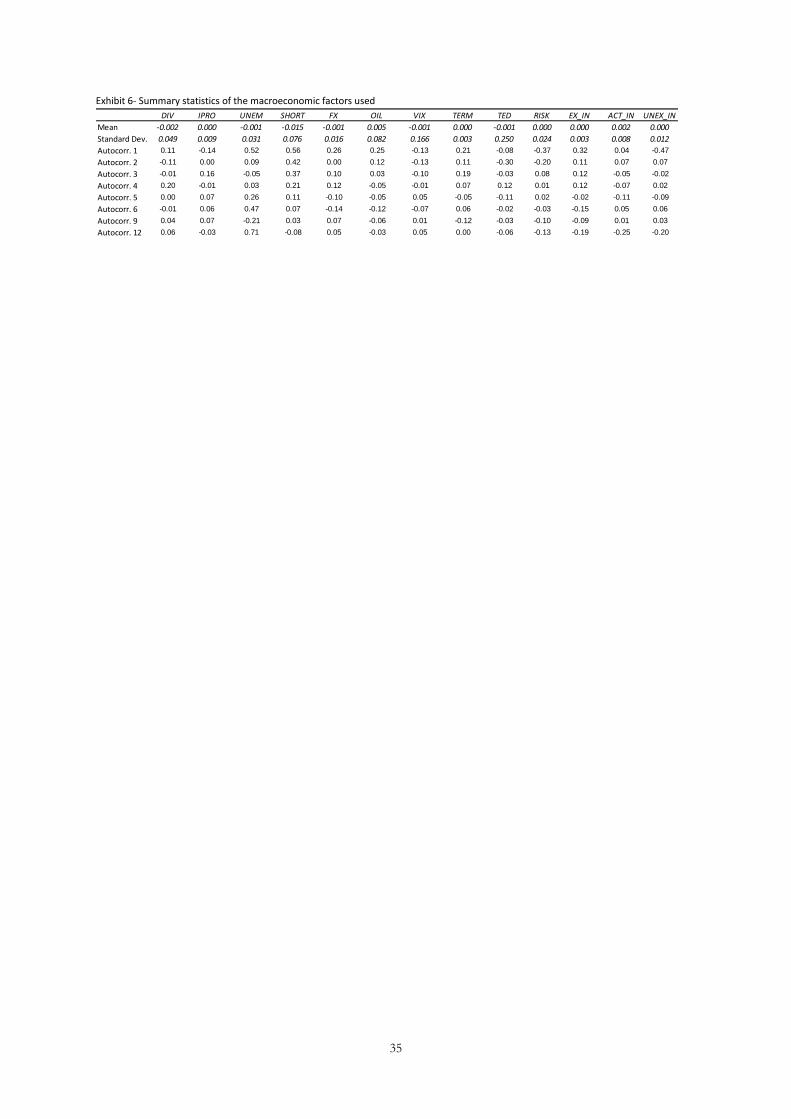
The tables Exhibit 4 show both the basic statistics and the correlation matrix for the 14 sub-asset

classes that are considered in paper. All the returns are calculated as log changes of the total

return indices of the assets4. Three are three equity sub-asset classes; U.K. Equities (E_UK),

Overseas Equities (E_OS) and Emerging Market Equities (E_EM). Also included are four fixed

income sub-classes; Gilts (B_GVT), bonds with greater credit link (B_GVT), Index-linked Gilts

(B_IL) and Overseas Bonds (B_OS). Both Listed Estate (REL) and Direct Real Estate (RE) are

included. Three types of commodities futures indices are studied, two diversified: C_GS and

C_RJ and also a gold index (GOLD). A diversified hedge fund index (HF) and an index based

on the returns of wine (WINE) are featured as well. Real estate, hedge funds and wine have

been desmoothed in order to compensate for their reduced volatility that has resulted from

valuation or illiquidity biases5.


As one might expect, the average monthly returns are substantially different across the different

asset classes with the maximum one being HFRI at 1.1% a month and the lowest one being the

Reuters/ Jefferies CRB index with a figure of 0.30%. Fixed income assets produced low levels

of variation in their total returns over time; gilts had a standard deviation of 0.169% this was

exceeded by most other assets. One must be careful with regard of the distributions of these

assets; all but the gilt index fail the Jarque-Bera test for normality at both 95% and 90%

confidence levels, whilst the gilt index only passes at 90%. Many of the indices are leptokurtic,

particularly RE and the Reuters/ Jefferies index. On the other hand the FTSE 100 and gilts

indices are extremely platykurtic. Most of the indices have varying levels of negative skewness.

Below one can also find the correlation matrix for the asset classes.


4 Please contact authors for more details on the asset classes and the proxies used.

5 These were each desmoothed differently; details are available on request.

7

4.2 Macroeconomic factors Macroeconomic factor variables such as ones used in the literature above are found not only to

explain asset class performance but as one may expect more generally they are indicators of

recent and future economic growth (Chen 1991). Below you can find a description of each

macro-economic variable included in this study as well as additional commentary on why it has

been included.

Change in Industrial production and other proxies for general economic conditions

Chen et al. (1986) uses both the industrial production month to month growth rate and yearly

growth rate both of which are led by one month. In Brooks and Tsolacos (1999) the rate of

unemployment tis used to reflect general economic conditions in the UK. In our preliminary

regressions we will include both unemployment and industrial production (lead by one month).

In both cases these were included in terms of the monthly log changes; the variable for industrial

production is denoted as IPRO while unemployment is UNEM.

Change in expected inflation

In many of the studies above inflation is spilt into different components, both expected and

unexpected inflation are included as separate variables. Geske and Roll (1983) suggest that equity

performance should be negatively related to expected inflation. Some research, such as Gorton

and Rouwenhorst (2006) suggests that commodities may be a better hedge against inflation than

equities or bonds. There are several methods suggested to calculate expected inflation as in

Chen et al. (1986), we use the Fama and Gibbons (1984) method to create their measure of

expected inflation. This is the difference between the T-bill rate and the fitted expected real rate,

where the expected rate is equally weighted moving average of the past 12 month’s ex post real

rates (T-bill minus CPI). This also compared this with a forecast from an ARIMA model and

the results were similar. Unlike Chen et al. (1986) we use the first differences in terms of

percentage point changes in yield of this variable to attempt to reduce autocorrelation. This

variable will be denoted as EX_IN. We also included actual inflation as measured by the

percentage change in the consumer price index (CPI) as ACT_IN.

Unexpected or unanticipated inflation (UNEX_IN)

Schwert (1981) suggests that for equities unexpected inflation contains new information on the

likely level of future expected inflation. He suggests that an increase in unexpected inflation is

likely to cause a transfer of wealth from bond holders to equity holders. In contrast to this,

Geake and Roll (1983) conclude that equities are negatively related to both unexpected and

8

expected inflation. Chen, Roll and Ross (1986) and others calculate this by subtracting the

realised monthly first difference in the log of the Consumer Price Index less the series of

expected inflation as calculated above. We use this approach and use the first differences of the

series in percentage points.

Changes in the risk structures of interest rates (RISK)

Chen et al. (1986) define this variable as the returns on a portfolio of Baa and under bonds less

the return on long-term government bonds. A measure for term and default is also used in

Fama and French (1992) to explain both stock and bond returns. Elton, Gruber, and Blake

(1995) suggest that higher default risks should affect corporate bond returns. Ferson and Harvey

(1991) note that their results in a pricing model were sensitive to the definition of this variable.

Due to this study being U.K. based, the closest proxy available was to use data from the Barclays

Capital fixed income index series. The data that was used was from bonds that formed the

Barclays Sterling non-Gilt AAA and BBB indices (mostly corporate bonds). There is a problem

with using this data; despite some adjustments there was still a duration mismatch between the

indices.

Changes in the term structures of interest rates (TERM)

This variable is included in many of the studies in the literature review above. There also has

been extensive additional work in in using the term structure of the yield curve to gain insight

into asset prices (Keim and Stambaugh 1986, Campbell 1987, Resnick and Shoesmith 2002).

Campbell (1987) uses the yield curve to predict the return on equities and finds a similar result;

that suggests that risk premia on T-bills tend to move fairly independently with equities whereas

taking 20 year bonds into account boasts the predictably. In Chen et al. (1986) they define this

as return on long-term government bonds less the period return on one month T-bills (lagged

one month). In this study the difference used was that between 10 year government bonds and

three month T-bills. The monthly change in percentage point terms of this rate was used.

Oil Prices (OIL)

Chen et al. (1986) point out that it is often argued that the oil price should be included in any list

of systematic factors that influence equity returns and pricing. In Amenc et al. (2003) the

authors consider the oil price to be related to short term business cycles. We have included the

monthly change in the price of Brent Crude (US $).

9

Short term interest rate factor (SHORT)

Ferson and Harvey (1993) and Roache (2008) include this as they suggest it can be used to

capture the state of investment opportunities there it is included in real terms. Again this is

included it as monthly changes to avoid problems associated with autocorrelation.

Stock market factor (DIV)

This is used in Elton et al. (1995) as a measure to reflect general economic conditions. However,

it is included in many other studies as the proxy for the market portfolio. We have used the

monthly change in the dividend yield on companies in the FTSE All-Share index as our stock

market factor. Dividend yield is used widely throughout the literature to attempt to predict the

returns of different asset classes.

Foreign Exchange factor (FX)

Ferson and Harvey (1993) include currency movements of G-10 countries versus the dollar.

Roache (2008) suggest that exchange rate risk may be priced by the stock market and that

commodities are argued by some to act as a hedge against a weak U.S. Dollar. Here we have

included the change in the logs of the UK GBP Sterling index effective exchange rate index

which is an index of the UK Pound’s performance versus other currencies on a trade weighted

basis.

TED Spread (TED)

Ferson and Harvey (1993) include this factor as they suggest that it may capture fluctuations in

credit risk. This indicator was also widely followed during the 2007 financial crises as it

represents to some extent the level of risk that is contained in the banking sector. It is calculated

as the difference between the three month LIBOR rate and the three month T-bill rate. To

reduce autocorrelation it is included in the change in the rate from the previous month in basis

point terms.

Change in the VIX Index (VIX)

The VIX Index (the Chicago Board Options Exchange Volatility Index) measures the implicit

volatility of options written on the S&P 500 index. This is included in the Amenc et al. (2003)

paper as a factor for hedge fund risk exposure. It can also be used as a general proxy for the

10

volatility or risk levels that are likely to seen in the U.S. equity market going forward and in a

wider context as a guide to the general level of risk aversion contained within world financial

markets. The change in the log of the VIX index is included.

A summary of the explanatory variables is included in Exhibits 5 and 6 below.

[INSERT EXHIBIT 6 + 7 HERE]

11

5. Methodology

5.1 Background

Firstly univariate regressions were carried out by regressing each asset class on each one of the

macroeconomic variables at lags zero to 12. Overall, the independent variables had the most

significance at lag zero. Thus the conclusion from this preliminary exercise was that it is worth

further investigating the all the variables at lag zero. In the next part of the process models were

created using some of the framework laid out in the existing literature. Six models were run

using variable combinations identified from the previous work6. Using these results and the

results from the univarate regressions, two final models were created.

5.2 The Basic Model Econometric Model

Ordinary least squares time-series regressions are run in order to get estimates for the risk

parameters. 14 different regressions were run; one for each of the sub-asset classes all of the

basic form below.

Where

the realised return on an asset i in month t, t = 1,…,228.

a constant for asset i.

the estimated sensitivity (factor beta) of to factor j, j =1,…,k (depending upon specific

model.

the measure for systematic factor i in month t and

= the residual for asset

In each case the dependent variable is one of the 14 sub-asset classes ( While the

independent variables ( are macroeconomic factors and the number of these depends on the

exact model that is being run but is between four and eight.

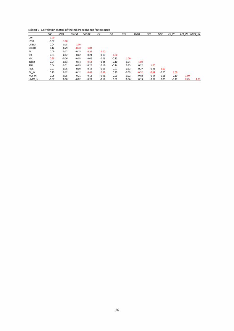
5.3 Multicollinearity issues

In Alexander (2008) the possibility that problems due to multicollinearity may arise in

fundamental factor models is directly addressed. The presence of multicollinearity does not tend

to affect the power of the model in overall term but it does affect individual regression

coefficients. These are estimated with reduced precision and the OLS estimator becomes less

efficient.

6 Results available on request.

12

There is no fully established statistical test for the presence of multicollinearity although it is

possible to roughly assess the likelihood of its presence by looking at the correlations between

the explanatory variables. In Exhibit 7 above the correlation matrix for the explanatory variables

is shown. It is clear that there are a number of correlation coefficients that could perhaps be

described to be high; the highest of these is the correlation coefficient between expected

inflation and short term interest rates of 0.66. This high correlation does make economic sense

as the expected inflation figure is based upon a forecast of short term interest rates. The next

highest is that between unexpected inflation and actual inflation (0.65). Two of the other high

correlations are between expected inflation and the change in term spreads of -0.52 and expected

inflation and the TED spread of -0.54. Expected inflation is also reasonably highly correlated

with the foreign exchange factor (has a coefficient of 0.39); perhaps a result of a common

interest rate effect. Change in the dividend yield and the change in the VIX index are

reasonability high correlated (the coefficient is 0.53) as are the change in unemployment and the

change in the short term interest rates (0.40), again these links are ones which one may expect.

From this analysis it may be possible to conclude that there may be some multicollinearity issues

that will arise especially from the two inflation variables. Many preliminary regressions were

performed using replicating ones from the existing literature and also by building up models by

adding in factors. By doing this it is possible to discover signs of multicollinearity, there were

substantial changes in the estimated regression coefficients when certain explanatory variables

were added to some models. The variables that caused notable changes within in the models

were (perhaps unsurprisingly) the inflation variables and also the combination of SHORT and

TERM. In order to correct for this multicollinearity problem the first decision made was to

drop both expected and unexpected inflation from the main model. We are effectively replacing

expected and unexpected inflation with actual (realised) inflation thus in theory the amount of

information lost should be minimised. Secondly, unexpected inflation appeared to have little

predictive power anyway thus removing will have little effect on the model’s power; however, it

is worth noting that expected inflation did appear to have somewhat more predictive power than

actual inflation. Secondly, TERM was included in the final model but SHORT was excluded as

its inclusion appeared to influence some of the betas.

13

5.4 The final models

For the final results, as stated previously; two new models are reported. One of these was

deemed to have the best explanatory power across all the asset classes whilst using the best

proxies and being as econometrically accurate as possible. This model included seven variables:

DIV, FX, OIL, VIX, TERM, ACT_IN and TED. The second was a version of this model that

was constrained to having four factors, as in Section 1 the results suggest that only four factors

may explain a great deal of the variation of the returns of the asset classes. The four factors that

were included are: DIV, SHORT, FX and OIL. Also reported for comparative purposes are the

models based upon the factors discussed in the papers; Chen et al. (1986) and Amenc et al.

(2003).

14

6. Results

6.1 The overall explanatory power of the models

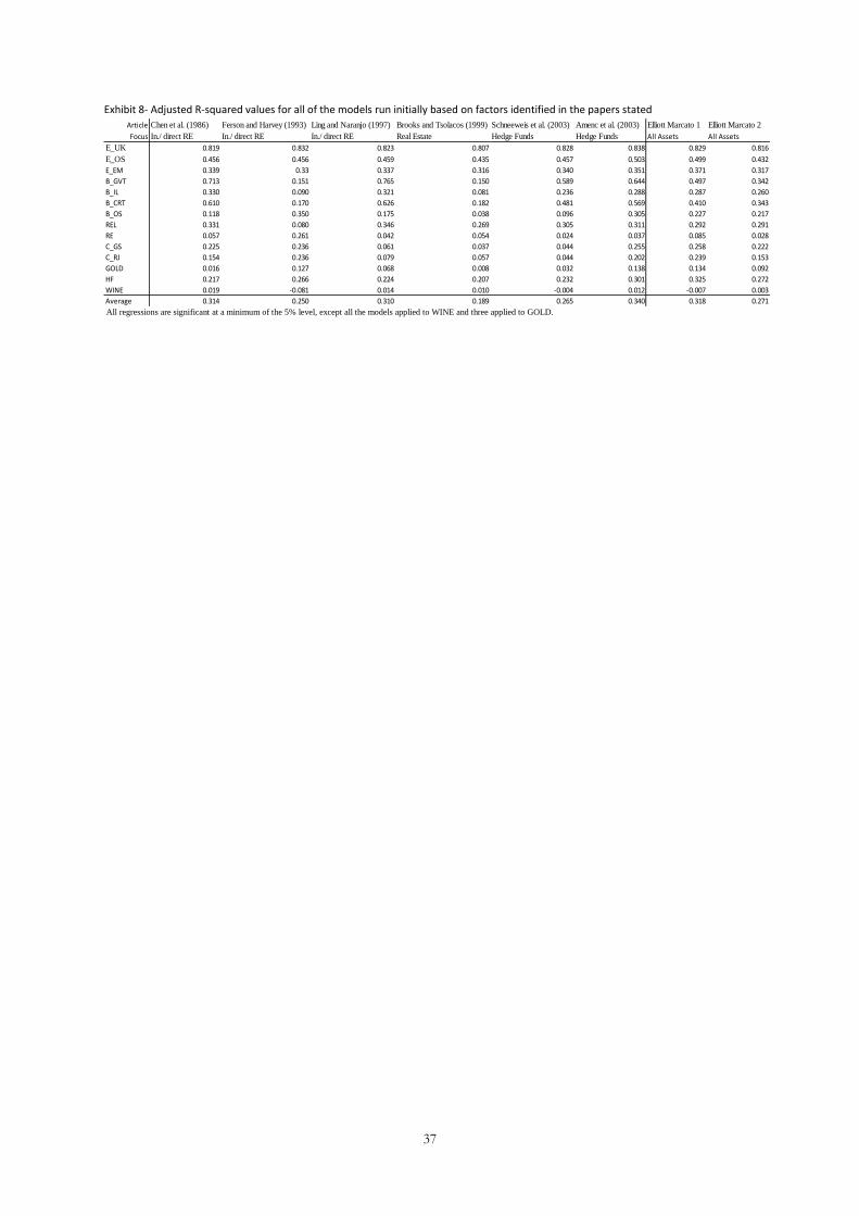
In Exhibit 8 a comparison of all the initial models is shown as well as the new models, the

adjusted R2 for each different is shown model for each of the sub-asset classes as well as a simple

average for all of them. All the models F-statistics are significant at the one percentage level

except are of the models when applied to wine and the Chen et al. (1986) model when Model

Three applied to gold. Generally the two best models were those using the factors identified in

Ferson and Harvey (1993) and in Amenc et al. (2003). These had an overall R2 of approximately

0.34 which is marginally higher than that of our full model (0.318) the model using the Chen et

al. (1986) factors and the Ling and Naranjo (1997) model. At the asset class level most of the

models had high explanatory power when related to equities sub-asset classes, whilst all expect

the one using factors based on Ferson and Harvey (1993) explained government bonds well.

The returns of index linked bonds were not explained particularly well by any of the models, the

maximum R2 here was 0.33 and models that included the change in expected inflation appeared

to perform best. Likewise all the models which included the change in the risk structure of

interest rates appeared to have a higher explanatory power in regard to the returns of corporate

bonds well than those that do not. The models that include them generally produced an R2 of

around 0.60. Overseas bonds are generally not explained very well by any of the models. Listed

real estate was generally explained fairly well were as conversely unlisted real estate was the asset

class that was explained the worst apart from wine. The two general commodity indices were

explained better by some models than others, the inclusion of OIL as a variable certainly

increased a model’s explanatory power while the inclusion of SHORT may also have increased it.

Hedge funds generally have an R2 in the low to mid-twenties; however this increases to the low

thirties in our main model and in Amenc et al. (2003); this may be a result of the inclusion of

VIX.


Although looking at the above results is an interesting exercise there are important caveats one

must consider. As discussed previously there is a multicollinearity problem with including the

variable expected inflation. Although this will not cause the overall models to be less reliable it

does affect the individual coefficients accuracy, thus we have removed it from our model.

Expected inflation does appear to be a better explanatory variable than actual inflation (which

15

was the alternative included in our model) thus the models that include it are likely to gain some

increased explanatory power from this variable. The first three models in table Exhibit 8 did use

both expected and unexpected inflation. The second problem with these results is that SHORT,

which was also not included in our models due to multicollinearity, has explanatory power

beyond TERM. Thirdly, we did not include the RISK variable in our models regarding which

may also have made some other models on occasion look superior to mine. As previously

discussed our proxy for this variable is noisy so it is likely to represent more than one economic

effect. In order to be as prudent as possible in terms of creating our final models we thus did

not include RISK. If this variable was included as well as the other eight in the model it would

it would increase the average R2 from 0.318 to 0.335. All of other the models in the above table

feature RISK except for Ferson and Harvey (1993).

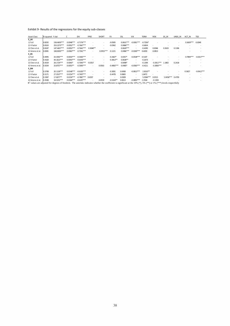
6.1 Equity

In Exhibit 9 below the detailed regression results for all four of the models are shown in

represent of each of the three equity sub-asset classes. The first major point to note is that all

the regressions are significant at the one percent level of significant and that there is little

deviation in terms of the R2 of the four models for all three of the assets. Also worth noting is

that there is perhaps evidence of multicollinearity in Model 4; the changes in the sign of the

variable TERM when compared with the other models may be an indicator of this.


The four models for U.K. equities all have a great deal of explanatory power with adjusted R2

values ranging from 81 to 83 percent. All the models have negative coefficients for dividend

yield that are significant at the 1% level. This is what one would expect in terms of these

coefficients, the dividend yield of the FTSE All-Share should have a large highly significant

effect on the total return of the All-Share index. This is because the dividend yield is calculated

as the dividend divided by the price, the total return is also made up of the dividend return as

well as the capital return so it is also directly a constituent of the total returns. As the price goes

up, the denominator of dividend yield goes up driving it lower as equity prices tend to rise much

faster than the dividend pay-out ratios this leads to a negative relationship between equities and

dividend yield which we see here. The SHORT variable is also significant at the 1% level in

Model 4, the sign being positive, this represents the fact that the opportunity cost of capital is

16

increasing and thus the return on equities should also increase. OIL is also significant at the 1%

level in each of the four models; it has a positive sign which may be surprising as it is a direct

cost to many firms and thus a rise in its price may reduce profitability. However; as the Oil and

Gas sector is the second biggest sector in the FTSE All-Share, making up over 17% of the index

(FTSE 2010), the benefits to this sector may cancel out the costs to other companies. Chen et al.

(1986) also found a positive link with the oil price. In the case of Model Three, industrial

production is significant with a positive sign at the 5% level which is economically feasible. In

Model One and Model Four which include VIX, this variable is significant at the 1% level with a

negative sign in both cases. As VIX can be thought of as an indicator of perceived risk within

the financial markets it tends to have a negative relationship with equities. The only other

variable that is significant in terms of U.K. equities is actual inflation in Model One (at the 10%

level); it has a positive sign which may imply that domestic equities may be a hedge against

domestic inflation.

In terms of general overseas equities the four models explanatory power is substantially less than

when they are applied to U.K. equities, here the R2 values range from 43% to 50%. This is to be

expected as the change in the FTSE dividend yield will have a larger effect on U.K. equities.

DIV is still significant at the 1% level in all four of the models; this supports the thesis that

world stock markets are connected. In this case SHORT is no longer significant in Model Three.

FX is significant at least the 10% level in the three models that include it; the negative sign here

is likely the result of the fact that as Sterling depreciates the returns in these overseas assets will

automatically be bigger in Sterling terms. Oil is only significant in two of the models, one at the

10% and the other at the 5% significance level. Again VIX is significant at the 1% level for both

models with a negative coefficient. In respect to overseas equities, in Models Three and Four

which contain it as a variable, RISK is significant at the 1% level. The coefficients have negative

signs suggesting that as the premium gained for holding lesser quality bonds over those with

higher credit ratings decreases, the return on overseas equities goes up; this may be a sign of

increased risk tolerance. In the 1st model now actual inflation is significant at the 1% level and

also TED is significant at 1%. The coefficient for TED has a negative sign, TED can be thought

of a measure of stress in the financial system, as this goes down it will encourage more risk

taking in the financial markets. Ferson and Harvey (1993) also find in their study that their TED

spread variable has a negative sign for most countries.

17

Finally addressing emerging market equities one can see in most cases the results are the same as

with developed market overseas equities. The same coefficients are significant for DIV, VIX

and TED. Only Model 4 has a significant coefficient for FX, perhaps implying that currency

moves are less responsible for the returns of emerging market equities to the U.K. investor. The

major differences are that RISK is no longer significant, and expected inflation and TERM are

significant in Model 1 and 4 at the 1% level.

6.3 Fixed Income

The results in respect to the four fixed income sub-classes are shown in Exhibit 10 below. Again

all the regressions are significant at the 1% level but in this case there is large deviation in terms

of the R2 of the four models for all each of the sub-asset classes. In addition to this there is a

large range of the explanatory power of the models between regarding different assets. Two

general points can be made, firstly, both government and U.K. credit exposed bonds are overall

better explained by some of the models than index-linked and overseas bonds. Secondly,

Models Three and Four which include the RISK variable in most cases have the most

explanatory power.


In general Gilts are explained by the three larger models reasonably well with approximate R2

between 0.50 and 0.71. There is a small significant coefficient for DIV which is significant at the

1% level for Models One, Two and Four and significant at the 10% for Model Three. This

implies that there is a slight positive performance between stocks and bonds which may be

contrary to some previous findings. SHORT is significant at the 1% level in Model 4 and has a

large negative coefficient, this is to be expected as when interest rates fall bond prices move

upwards. The foreign exchange variable is significant in all three of the models that include it, it

has a negative beta, and this may suggest that the pound weakens due to falling interest rates

which have a positive for bond prices. OIL has a small significant negative coefficient which is

significant in all of the four models; this may be the result of oil prices being inflationary. The

coefficient for VIX is small and positive for the two models that include it and is significant at

least the 10% level, as investors tend to buy government bonds when they are being risk adverse

this effect is intuitive. TERM is significant at the 1% level in all four models. The coefficient is

negative which suggests as the yield curve gets steeper that bonds prices fall, this may be the case

18

as the rates on the longer duration bonds may be rising this their prices will be falling. Elton,

Gruber, and Blake (1995) state that interest rate changes are the major cause of the changes in

bond portfolios. RISK is also highly significant in the two models that feature it, here the sign is

positive, this may be expected as when there is less demand for risky bonds there tends to be

more demand for government ones. In the main model TED is significant at the 1% level with a

positive sign as with VIX as, in this case financial sector, risk is deemed to be higher the demand

for Gilts should increase. Surprisingly unexpected inflation is not significant; Elton, Gruber, and

Blake (1995) find a negative relationship with this variable. However expected inflation is

significant in Model Three at the 1% level and actual inflation is Model One at the 1% level.

Both these variable’s signs are negative as higher inflationary expectations or higher realised

inflation will have a negative impact on bond values (via expected increased interest rates).

Cambell and Ammer (1993) make the point that increases in long-run expected inflation tend to

drive the bond market down.

Out of the four fixed income assets, the models overall had the second least explanatory power

in respect to index-linked bonds, generally overseas bonds were the most difficult to explain. For

the most part the results for index-linked Gilts were largely similar to normal Gilts: DIV, TERM,

FX and TED had much the same results. SHORT was now only significant at the 10% level.

RISK was no longer significant in any of the models which may be surprising. Realised inflation

was not found to have a significant affect upon the returns of index-linked bonds; this is

unanticipated since these securities’ prices are adjusted to take account of inflation there should

be a positive relationship. However; there are two reasons why no link may have been

established, firstly; the inflation figures we have used for realised inflation are based on the CPI

(RPI is used in the index-linked calculation). Secondly, there the way that the inflation

adjustment is applied to the prices if index-linked gilts mean that there is either a three or an

eight month lag in the inflation protection. Expected inflation; however, was significant at the

1% level, it has a smaller coefficient than normal Gilts but it is still negative. This negative sign

is difficult to explain, even given the problems discussed above. In Reschreiter, (2003) a negative

link is suggested of inflation linked bonds and unexpected inflation, although, this is easier to

justify than with unexpected inflation.

Following on from these results for inflation-linked bonds, the results for bonds with higher

credit risk are very alike although the models had much higher R2. The only real different in the

significance level of the betas relates to SHORT and FX. Unlike both types of Gilts there is no

19

longer a significant relationship with FX except at the 5% level in Model Four. Only different

are that RISK and ACT_IN are significant; although these results are comparable to those

produced in relation to normal Gilts.

The results for overseas bonds are in many ways the most different from the other fixed incomes

sub-classes. Firstly DIV is no longer significant for any of the models. IPRO has a large

negative beta (1% level); this is hard to interpret due to the international nature of the returns.

The variable SHORT does have a significant negative coefficient, while OIL is not significant.

FX is highly significant with large negative coefficient values, as with foreign equities. The

coefficient for EX_IN is comparable to those for the other three asset classes. While TERM is

highly significant for Models Three and Four and not significant for Models One and Two, this

may be a result of effects of multicollinearity. Perhaps a surprising result is that whilst still

significant at 5% for both models; RISK now has a negative sign. This may suggest that this may

be an asset class which be less highly rated and thus an increase in the risk premium may hurt the

price.

6.4 Real Estate

The results from the two real estate sub-classes are shown in Exhibit 11. All four models have

F-statistics that are significant at the 1% level for both sub-asset classes, except the application of

Model Three to listed real estate (significant at the 5% level). Each of the four models also has a

very similar R2 in regard to listed real estate (between 0.29 and 0.33). The R2 for direct real estate

were very low ranging from 0.028 to 0.085, demonstrating that none of the models have much

explanatory power.


Like with the results of diversified U.K. equities, listed real estate has a large negative beta for

DIV which was significant at the 1% level in all four of the models. This follows from the fact

that these are a type of equity and thus will be subject to more general equity market movements.

Also significant at the 1% level in Model Four is SHORT; again this reflects that the investment

opportunity cost is increasing. However, it is interesting that both TERM and RISK are not

significant as these firms tend to use leverage. There is a positive beta for IPRO that is

significant at the 1% level; perhaps as generally increasing production will lead to a demand for

buildings. OIL was significant at a minimum of the 5% level of significance in all four models,

20

this result is unexpected. TERM is significant in three out of the four models that feature it,

thus implying that real estate tends to do well in times where credit risk is perceived to be low.

Chan et al. (1990) found that changes in term structure were important in explaining listed real

estate returns although there are also contradictory results. In Model Three expected inflation is

highly significant with a negative beta, this may contradict some research that both equities and

real estate protect against inflation (including Chen et al 1997) or alternatively that there is no

significant link either way (Chan et al. 1990).

The results for direct estate were not as one way expect due to the fact that they had very low

explanatory power. It is very possible that this may be a result of the unsmoothing process and

this will be investigated later in this article. The only significant betas at a maximum of the 5%

level are TED (Model One), EX_IN (Model Three) and OIL, in three out of four models. TED

has a large negative coefficient and thus it may suggest that real estate performs well during an

environment of stable banking markets. EX_IN has a positive beta which may imply that real

estate may perform better in inflationary periods. In their study Brooks and Tsolacos (1999) use

listed real estate returns net of stock market influences (thus a proxy of the direct market), they

find no main macroeconomic variables have any significant explanatory power for this index.

6.5 Commodities

All the four models have F-statistics that are positive at the 1% level for both of the diversified

commodity indices. Our main model has slightly more explanatory power (R2 of 0.26) for the

GSCI than for the Reuters Jefferies index (R2 of 0.24). This general relationship is the same for

the other three models as well.


The GSCI index shows negative significant coefficients (two out of four at the 5% level plus one

at 10%) with DIV. This may suggest that as companies do well that they may increase the

demand for and thus price of, commodities. This finding is unlike Bailey and Chan (1993) which

finds no connection with a general stock market index. SHORT is also significant in Model

Four. As these indices are made up of fully collateralised futures, there will be an element of a

return from interest. FX is significant at the one percent level for two of the three models that

include it; in addition the other is significant at 5%. The beta here is negative and this is likely

21

because all commodities are priced in terms of U.S. Dollars. In Erb and Harvey (2006) the

authors also find a significant beta with respect to a foreign exchange factor as does Roache

(2008). OIL is significant at the one percent level in all of the models. The fact that oil futures

make up a large part of this index, it is logical that there will be a large positive beta with the

change in the spot price of oil. In the two models that include it, there is a negative coefficient

(one is significant at the 1% level) with RISK suggesting that commodities may perform better in

when there is less expectation of risk in the bond market. Likewise there is a negative coefficient

with TED. Although the beta with expected inflation is not significant both, unexpected

inflation and actual inflation have positive significant coefficients; expected at the 5% level and

actual at the 1% level. Gorton and Rouwenhorst (2006) find a basic positive relationship

between commodity futures and all three types of inflation included in this study.

The results for the Thomson Reuters/Jefferies CRB index are alike those for the CSCI; the betas

for DIV, RISK and TED are similar but significant at a stronger level while FX’s significance

level is the same. SHORT is no longer significant which is an unexpected result. The betas for

OIL are also highly significant but lower than those with the GSCI; this is because the CRB is a

more balanced index whilst the GCSI is more energy focused. Again unexpected inflation is

significant at the 5% level but in this case actual inflation is slightly less significant (at the 5%

level). Like with the GSCI above no significant results are found with the TERM variable this

finding is supported by that in Bailey and Chan (1993).

Addressing the results for gold it is apparent that for models One, Two and Four the regression

results are significant at the 1% level, although the F-statistic is not significant using the Chen et

al. (1986) factors. This may suggest that FX is a major explanatory factor for gold. The R2 are

low, the best being 0.14 in Amenc et al. (2003). The coefficient for SHORT is significant with

negative betas; this suggests that as short term fall gold becomes more valuable; this could be a

link between higher gold prices in deflationary environments. All the betas are significant for the

FX factor at the 1% level; again this is because gold is priced in U.S. Dollar terms. In Model

One there is a large negative, highly significant beta in regard to TED this may suggest that gold

may be desired during times of financial crises. Likewise in Model Four there is a significant

negative beta with RISK. None of the inflation variables are significant which may challenge

some opinions that gold is a good hedge against inflation.

22

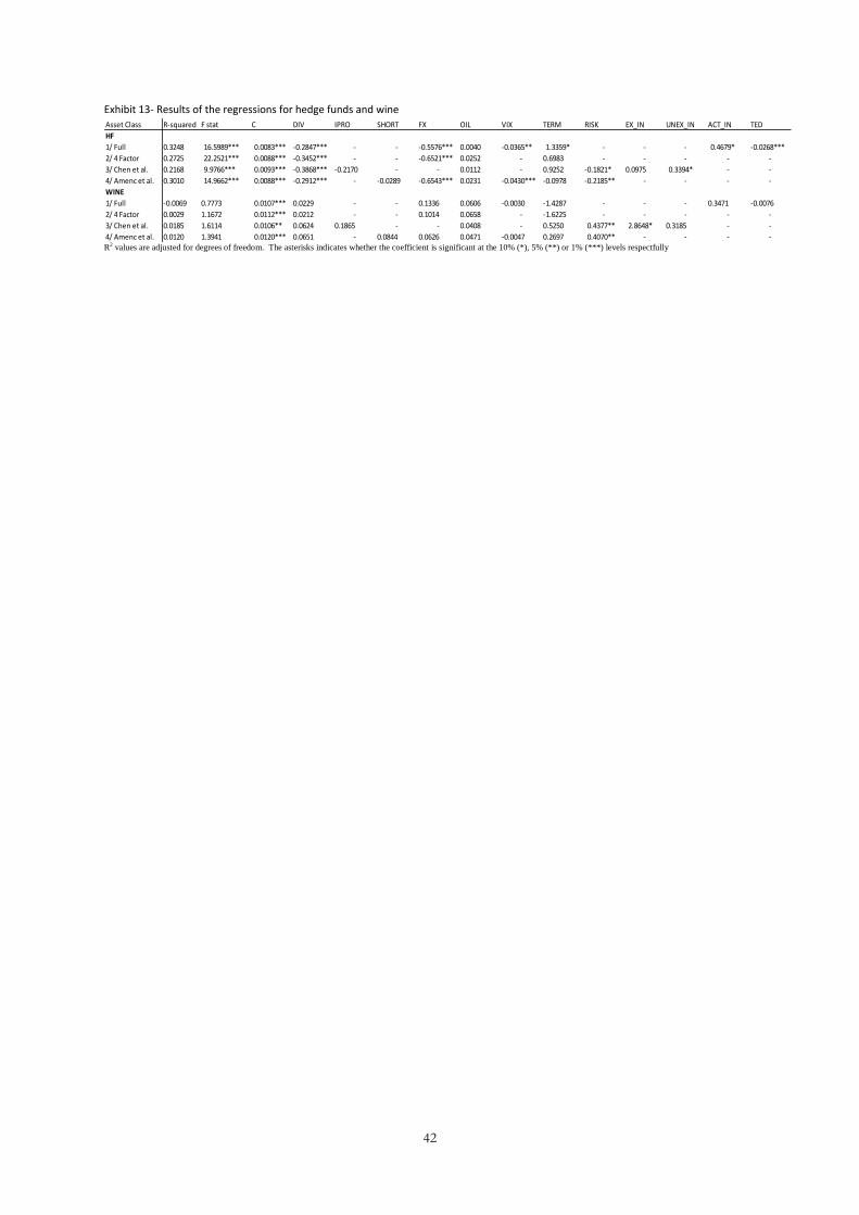
6.6 Hedge Funds

The results for hedge funds are shown in Exhibit 13; all four models have F-statistics that are

positive at the 1% level. Model One has an R2 of 0.33 while Model Four has one of 0.30; the

four factor model also has reasonable explanatory power at 0.27. DIV is significant in all the

models at the 1% level with negative betas, as many hedge funds hold long equity positions this

is understandable. Also significant with negative betas in all the models at the 1% level, is FX.

This result will be due to the vast amount of hedge fund positions being in U.S. and other

foreign currency terms. In the two models that feature it VIX is significant at least the 5% level

of significance with negative betas. Thus as volatility increases hedge funds perform less well,

this is intuitive as this is a diversified index; however, it is likely that some individual funds or

strategies will perform better if volatility increases. In Schneeweis, Kazemi and Martin (2003),

the authors find that all the hedge fund sub-indices a negative coefficient with VIX, except

convertible bond arbitrage. TED has a negative coefficient (with is significant at the 1% level),

thus this also suggests that hedge funds returns tend to decrease it times of financial risk. There

is also a negative relationship with RISK which is also true in Schneeweis, Kazemi and Martin

(2003). There is also a positive, significant beta with actual inflation which is perhaps is

unintuitive although only at the 10% level.


6.7 Wine

Looking at Exhibit 13 it is clear that the returns of wine are not explained by any of models.

Each of the models has an F-statistic which is not significant at the 10% or higher level. Thus

the returns on wine appear to be driven by factors that are not included in any of these models.

6.8 Unadjusted Indices

In Exhibit 14 below the results of using the factor models on the original versions of the indices

that were included as desmoothed versions above are shown. It is useful to compare these with

the adjusted versions in order to see how the desmoothing process has affected the regression

results.


23

Real Estate (Unadjusted Index)

When the factor models were applied to the desmoothed real estate index all four models had

even little explanatory power. The best model was Model One with an R2 of 0.09. Overall only

the adjusted returns for wine were explained by the four models to an even less extent. The

results for the unadjusted indices; however, are different to these. Firstly the first three models

have slightly higher explanatory power; all with R2 in the region of 0.15. Model Four; however,

has a much higher R2 of 0.41. Considering Models One, Two and Three the variables that are

generally significant are: DIV, TERM and FX. These results suggest that a negative relationship

with DIV and TERM and a positive one with FX are some of the factors driving the returns. All

of these are feasible relationships with the stock market factor a proxy for firm health and a

flattening yield curve good for financing opportunities. The result using the adjusted series

found the FX variable and expected inflation to be significant; none of these betas are significant

when the models are applied to the original unadjusted index data. This may prove that in this

case the desmoothing techniques that were used on the real estate data in order to correct for the

understated volatility has also changed the econometric structure of the returns. The

desmoothing technique used for the hedge fund data was the most severe and it also changed the

mean of the returns so perhaps this is unsurprising. What is most interesting is Model 4; here

the very large R2 is being driven by SHORT. This is likely to be the result of another problem,

which is that since the original index returns are highly autocorrelated and SHORT is the most

autocorrelated explanatory variable the large R2 values may be a result of this autocorrelation.

Thus the regression results may be biased anyway in the case. Secondly, in model Four there is

the peculiar result that TERM is significant but with a positive beat whilst Models One, Two and

Three have negative betas. This is likely to be a result a multicollinearity effect as SHORT is

included although with TERM.

Hedge Funds (Unadjusted Index)

Desmoothing the hedge fund index has some effect on the results of the regressions. In this

case the R2 values are higher when the models are applied to the desmoothed index rather than

the unadjusted one, for example the R2 for Model One was 0.32 using the desmoothed data,

while it was 0.27 using the original index data. Here the increased volatility structure of the

returns may help price discovery and thus increase the model’s power. One of the only

coefficients to vastly change their significance levels from using adjusted to original index data

are using the original data is RISK. This is now significant at a minimum of the 5% level in the

two models where it is a variable, were as it was not significant using the desmoothed series. It is

24

possible that this result may have been a consequence of the fact that there the original series is

autocorrelated and thus this result does not appear in when the desmoothed data is analysed.

VIX is no longer significant using the original data whereas it significant in both models that

include it at the 1% level using the desmoothed data. This suggests that by desmoothed the data

and thus adding volatility to it, there is now a connection to the VIX index which is a measure of

equity market volatility.

Wine (Unadjusted Index)

When the models are applied to the unadjusted wine index there is little difference between the

results.

25

7. Conclusion

The purpose of this study was to attempt to build up a better understanding of how a wide range

of asset classes react to changes in macroeconomic factors in respect to returns to a U.K. based

investor. After a long process a seven factor model and a four factor model were designed in

order to best explain the asset class returns whilst being as econometrically correct as possible.

The seven factor model had a simple average R2 of 0.32 over the 14 asset classes. This value

varied considerably from asset to asset. Some of the more traditional sub-asset classes had were

explained reasonably well, for example U.K. equities (R2 is 0.83), developed market overseas

equities (0.50) and U.K. government bonds (0.50). Emerging market equities (0.37), Index-

Linked (0.29) and overseas bonds (0.23) were explained less well. Listed real estate had an R2 of

0.29 but directly held real estate returns were very poorly explained by the models both in

original and desmoothed terms. Out of the ‘alternative assets’; hedge funds had the highest level

of explanatory power at 0.33, commodities were fairly low, while gold was the second lowest at

0.13. The returns of wine were not explained at all by the models, this result should be

investigated further in the future. Direct real estate, gold and wine appear not to be driven by

traditional economic variables at least not in a linear way. These may thus have portfolio

diversifying benefits, although further investigation is required

Generally dividend yield and the change in terms spreads were the factors that had the most

influence on the assets; however, these were not significant for all sub-asset classes. The change

in the oil price and a foreign exchange factor were the next influence and these four factors

made up the reduced models. Some of the other variables were important in explaining a

particular asset classes’ returns. Most of the individual coefficient results were supported by the

existing literature or had economic logic but some warrant further investigation.

An important point that was highlighted is that the choice of desmoothing method appears as if

it can considerably affect the results of factor analysis work. This is worth noting for future

work.

This information can be used to better understand what asset classes are likely to do during

different economic environments. It gives a better understanding to the relationship in the asset

correlation matrix. For example the correlation of 0.44 between overseas bonds and overseas

equities is at least partly driven by the fact they are independently driven by the foreign exchange

factor (as one may have hypothesised).

26

8. Further Work

In addition to be points raised above in term of specific results that may warrant further

investigation, this work with be improved by using a more complex method. Firstly,

investigating how the regression coefficients change over time may be worthwhile. Secondly,

initial Granger Causality tests suggest that there may be justification for the application of a

vector autoregression (VAR) technique to this data set.

27

References

Agarwal, V., and N. Naik, (2004), “Risk and portfolio decisions involving hedge funds”, Review of Financial Studies, 17 (1), 63-98. Alexander, C., and A. Dimitriu, (2005) “Rank Alpha Funds of Hedge Funds,” The Journal of Alternative Investments, Fall Alexander, C. (2008), Practical Financial Econometrics, Wiley, New York. Amenc, N., S. El Bied, and L. Martellini. (2003), “Predictability in Hedge Fund Returns." Financial Analysts Journal, Vol. 59, No.5 pp. 32-46. Avramov, D., Kosowski R., Naik N. Y., and M. Teo, (2010),”Hedge Funds, Managerial Skill, and Macroeconomic Variables”, Journal of Financial Economics, Forthcoming. Bailey, Warren, and K.C, Chan, (1993), "Macroeconomic Influences and the Variability of the Commodity Future Basis," Journal of Finance, vol. 48, no. 2 (June): 555-573 Ben Dor. A., L. Dynkin, and A. Gould. (2006), "Style Analysis and Classification of Hedge Funds." The journal of Alternative Investments. Vol. 9. No. 2 pp. 10-29. Brooks, C. and S. Tsolacos. (1999) ,“The Impact of Economic and Financial Factors on UK Property Performance”, Journal of Property Research, 16: 139–152. Campbell, J.Y. and Ammer, J. (1993), “What Moves the Stock and Bond Markets? A Variance Decomposition for Long-Term Asset Returns,” Journal of Finance, 48, 3-37. Capocci. D.and Hubner. G. (2004), “Analysis of hedge fund performance” Journal of empirical finance, Vol 11, pp. 55-80. Chan, K.C., Patric Hendershott, and Anthony B. Sanders, (1990), “Risk and Return on Real Estate: Evidence from Equity REITs,” AREUEA Journal, 18, 431-452. Chen, S., C. Hsieh and B. Jordan. (1997), Real Estate and the Arbitrage Pricing Theory: Macrovariables vs. Derived Factors. Real Estate Economics, 25: 505–523. Chen, N., R. Roll and S. Ross. (1986), “ Economic Forces and the Stock Market: Testing the APT and Alternative Asset Pricing Theories”, Journal of Business, 59: 383–403. Dumas, Bernard, and Bruno Solnik, (1995). "The World Price of Foreign Exchange Risk.", Journal of Finance, vol. 50, no. 2(December):445-477. Elton, E. .J., M. .J. Gruber, and C. Blake. 91995), “Fundamental Economic Variables, Expected Returns, and Bond Fund Performance.” Journal of Finance, Vol. 50, No. 4 1229-1256. Erb, C., and C. Harvey. (2006), “The Tactical and Strategic Value of Commodity Futures,” Financial Analysts Journal, March/April, 69–97. Estrella, Arturo (2005): “Why Does the Yield Curve Predict Output and Inflation?”, Economic Journal, Vol. 115, Issue 505, p.722-744

28

Estrella, A. and Hardouvelis, G. (1991), “The term structure as a predictor of real economic activity”, Journal of Finance, 46(2), 555±76. Fama, E. and French, K. (1988), “Dividend Yields and Expected Stock Returns,” Journal of Financial Economics, 19, 3-29. Fama, E. and French, K. (1989), “Business Conditions and Expected Returns on Stocks and Bonds,” Journal of Financial Economics, 25, 23-49 Fama, Eugene F. and Kenneth R. French, (1992), “The Cross-Section of Expected Stock Returns,” The Journal of Finance, Vol. 47, No. 2, pp. 427–465. Ferson, W. and Harvey, C. (1991), “The variation of economic risk premiums”, Journal of Political Economy, 99, 385-415. Ferson, W., and C. Harvey, (1993), “The risk and predictability of international equity returns”, Review of Financial Studies, 6, 527- 566. FTSE (2010) http://www.ftse.com/Indices/UK_Indices/Downloads/FTSE_All-Share_Index_Factsheet.pdf Fung, William, and David A. Hsieh, (1997), “Empirical Characteristics of Dynamic Trading Strategies: The Case of Hedge Funds”, The Review of Financial Studies 10, 275-302. Fung, W., Hsieh, D., (2004), “Hedge fund benchmarks: a risk based approach”, Financial Analysts Journal, 60, 65-80. Gorton, G., and K.G. Rouwenhorst (2006) “Facts and Fantasies about Commodity Futures”, Financial Analysts Journal, 62, 47{68. Harvey, C. (1995), “Predictable risk and returns in emerging markets”, Review of Financial Studies, Fall, pp. 773–816. Kat, H.M., Oomen, R.C.A. (2007). “What every investor should know about commodities part II: multivariate return analysis”, Journal of Investment Management, 5(3), 1-25 Ling, D. and A. Naranjo. (1997), “ Economic Risk Factors and Commercial Real Estate Returns”, The Journal of Real Estate Finance and Economics, 14: 283–307. Liow, K.H. (2004), "Time-varying macroeconomic risk and commercial real estate: an asset pricing perspective", Journal of Real Estate Portfolio Management, Vol. 10 No.1, pp.47-58. McCue, T. E. and J. L. Kling, Real Estate Returns and the Macroeconomy: Some Empirical Evidence from Real Estate Investment Trust Data, 1972–1991, Journal of Real Estate Research, 1994, 9:2, 277–87. Reschreiter, A, (2003), “Risk factors of inflation-indexed and conventional government bonds and the APT”, Money, Macro and Finance (MMF) conference, 2003 Roache, Shaun K (2008), "Commodities and the Market Price of Risk," IMF working paper WP/08/221

29

Schneeweis , Hossein, Kazemi , and Martin, (2003), “ Understanding Hedge Fund Performance: Research Issues Revisited—Part II”, The Journal of Alternative Investments, Spring 2003, Vol. 5, No. 4

30

Exhibits

Exhibit 1- Principle Component Analysis of All Asset Classes

sses

Value PC 1 PC 2 PC 3 PC 4 PC 5 PC 6 PC 7 PC 8 PC 9 PC 10 PC 11 PC 12 PC 13 PC 14

Eigenvalue 0.01 0.01 0.00 0.00 0.00 0.00 0.00 0.00 0.00 0.00 0.00 0.00 0.00 0.00

% of variation 39.46 17.18 12.18 9.73 6.96 5.08 2.87 2.08 1.78 0.99 0.78 0.51 0.32 0.07

Cumulative % 39.46 56.64 68.82 78.55 85.51 90.59 93.46 95.54 97.32 98.31 99.09 99.61 99.92 99.99

Eigenvectors:

E_UK 0.24 0.38 -0.04 -0.03 0.13 -0.06 0.23 -0.10 -0.63 0.11 -0.25 -0.48 0.10 -0.04

E_OS 0.38 0.15 -0.15 0.12 0.00 -0.14 0.56 -0.31 0.04 -0.09 0.49 0.29 -0.19 -0.03

E_EM 0.52 0.24 -0.27 0.37 0.25 0.12 -0.53 0.19 0.17 -0.07 0.16 -0.12 0.01 0.00

B_GVT 0.01 0.04 0.00 -0.02 -0.10 -0.13 0.03 0.49 -0.14 -0.03 -0.03 0.11 -0.41 -0.72

B_IL 0.04 0.05 0.04 -0.05 -0.09 -0.04 0.09 0.49 -0.26 -0.21 0.24 0.30 0.69 0.05

B_CRT 0.03 0.07 0.02 -0.03 -0.05 -0.06 0.05 0.44 -0.20 -0.07 -0.06 0.11 -0.52 0.68

B_OS 0.15 -0.19 -0.09 0.02 -0.34 -0.20 0.33 0.31 0.43 0.02 0.05 -0.61 0.10 0.06

REL 0.23 0.55 0.28 -0.52 -0.40 -0.10 -0.22 -0.10 0.24 0.02 -0.04 0.08 0.01 0.01

RE 0.05 0.10 0.19 0.03 -0.12 0.92 0.25 0.12 0.06 0.09 0.05 -0.05 -0.05 -0.05

C_GS 0.41 -0.41 0.37 -0.41 0.43 -0.03 -0.03 0.10 -0.02 0.35 0.18 -0.02 -0.02 0.00

C_RJ 0.33 -0.27 0.10 -0.14 0.03 0.10 0.04 -0.12 0.00 -0.79 -0.36 -0.01 -0.03 -0.04

GOLD 0.28 -0.41 -0.15 0.06 -0.64 0.08 -0.27 -0.18 -0.40 0.17 0.10 0.04 -0.04 0.01

HF 0.31 -0.03 -0.16 0.16 -0.02 -0.04 0.21 0.08 0.19 0.37 -0.66 0.42 0.15 0.02

WINE 0.06 0.03 0.77 0.60 -0.11 -0.18 -0.01 -0.04 -0.03 0.00 -0.02 -0.02 0.01 0.00

31

Exhibit 2- Principle Components Explaining Variances of All Asset Classes

1 2 3 4 5 6 7 80

10

20

30

40

50

60

70

80

90

100

Principal Component

Variance E

xpla

ined (

%)

0%

10%

20%

30%

40%

50%

60%

70%

80%

90%

100%

32

Exhibit 3- Summary of the macroeconomic factors used in the most relevant literature

Reference Asset Class Geo.

∆ in

indu

stri

al p

rodu

ctio

n or

sim

ilar

Con

sum

ptio

n

Rat

e of

une

mpl

oym

ent

∆ in

une

xpec

ted

infl

atio

n

∆ in

exp

ecte

d in

flat

ion

Exp

ecte

d in

flat

ion

∆ in

ris

k pr

emia

of

inte

rest

rat

es

∆ in

term

str

uctu

re o

f in

tere

st r

ates

Yie

ld o

n 3

mon

th T

-bill

s

TE

D s

prea

d

Oil

Pri

ces

Sto

ck m

arke

t Fac

tor

(inc

. div

. yie

ld)

inde

x of

agg

rega

te b

ond

retu

rns

mor

tgag

e se

c.re

lativ

e go

vt. b

onds

∆ in

the

VIX

inde

x

A f

orei

gn e

xcha

nge

mea

sure

Mar

ket v

olum

e

Chen et al. (1986) Equities US r r r r r r r r

Ferson and Harvey (1993) Equities Global r r r r r r r

Elton et al. (1995) Fixed Income US r r r r r r r

Chan et al. (1990) Indirect RE US r r r r r r

Chen et al. (1997) Indirect RE US r r r r r

Ling and Naranjo (1997) In./ direct RE US r r r r r r r r r

Brooks and Tsolacos (1999) Indirect RE UK r r r r

Bailey and Chan (1993) Commodities US r r r r r r

Roache (2008) Commodities US r r r r

Schneeweis et al. (2003) Hedge Funds US r r r r

Amenc et al. (2003) Hedge Funds US r r r r r r r r

Explanatory Variables included

33

Exhibit 4- Summary statistics of the sub-asset classes

E_UK E_OS E_EM B_GVT B_IL B_CRT B_OS REL RE C_GS C_RJ GOLD HF WINE

Mean 0.007 0.006 0.018 0.007 0.006 0.007 0.006 0.004 0.008 0.003 0.003 0.005 0.010 0.011

Standard Dev. 0.042 0.044 0.064 0.016 0.019 0.015 0.019 0.061 0.040 0.062 0.038 0.043 0.028 0.058

Kurtosis 1.111 2.734 3.617 0.744 4.348 1.134 0.437 2.512 6.756 3.420 9.613 2.531 2.432 11.680

Skew -0.753 -1.073 -1.039 -0.133 0.162 -0.395 0.090 -0.524 -0.575 -0.748 -1.404 -0.003 -0.718 1.204

Autocorr. 1 0.11 0.13 0.26 0.08 0.04 0.12 0.13 0.23 0.06 0.22 0.22 -0.13 -0.02 -0.12

Autocorr. 2 -0.07 -0.01 0.23 -0.10 -0.27 -0.07 -0.08 0.00 -0.10 0.06 0.18 -0.04 0.07 0.10

Autocorr. 3 0.00 0.11 0.15 0.10 0.01 0.09 0.00 0.08 0.20 0.15 0.16 0.02 -0.01 0.19

Autocorr. 4 0.18 0.09 0.08 0.03 0.10 0.10 -0.08 0.22 -0.10 0.06 0.14 -0.01 0.06 -0.02

Autocorr. 5 0.02 0.04 0.02 -0.02 0.08 0.02 -0.13 0.11 -0.04 0.04 -0.05 0.00 -0.04 0.12

Autocorr. 6 -0.04 -0.07 -0.06 -0.09 -0.11 -0.03 -0.06 -0.10 0.16 0.03 -0.07 -0.01 0.03 0.04

Autocorr. 9 0.03 -0.02 0.09 0.01 0.03 -0.03 0.13 0.01 -0.03 -0.08 -0.17 -0.06 0.07 0.01

Autocorr. 12 0.06 0.07 0.03 -0.01 -0.03 -0.05 -0.12 0.03 0.22 -0.17 -0.22 0.08 -0.06 -0.04

34

Exhibit 5- Correlation matrix of the sub-asset classes

E_UK E_OS E_EM CASH B_GVT B_IL B_CRT B_OS REL RE C_GS C_RJ GOLD HF WINE

E_UK 1

E_OS 0.70 1.00

E_EM 0.64 0.76 1.00

CASH 0.02 0.02 0.09 1.00

B_GVT 0.16 0.03 0.04 0.20 1.00

B_IL 0.30 0.20 0.14 0.04 0.66 1.00

B_CRT 0.38 0.15 0.17 0.14 0.86 0.67 1.00

B_OS -0.05 0.44 0.23 0.10 0.27 0.21 0.12 1.00

REL 0.59 0.36 0.28 -0.10 0.23 0.33 0.36 0.01 1.00

RE 0.13 0.06 0.11 -0.13 -0.15 0.11 0.06 -0.12 0.20 1.00

C_GS 0.16 0.36 0.32 -0.01 -0.07 0.14 0.02 0.32 0.14 0.04 1.00

C_RJ 0.21 0.53 0.47 -0.04 -0.09 0.14 0.00 0.49 0.14 0.12 0.82 1.00

GOLD -0.04 0.35 0.32 -0.10 0.03 0.10 -0.05 0.65 -0.03 0.02 0.39 0.62 1.00

HF 0.49 0.80 0.78 0.11 0.08 0.13 0.13 0.57 0.15 0.06 0.44 0.61 0.53 1.00

WINE 0.02 0.05 0.06 -0.08 0.01 0.08 0.07 -0.01 0.08 0.17 0.12 0.08 -0.01 0.04 1.00

35

Exhibit 6- Summary statistics of the macroeconomic factors used

DIV IPRO UNEM SHORT FX OIL VIX TERM TED RISK EX_IN ACT_IN UNEX_IN

Mean -0.002 0.000 -0.001 -0.015 -0.001 0.005 -0.001 0.000 -0.001 0.000 0.000 0.002 0.000

Standard Dev. 0.049 0.009 0.031 0.076 0.016 0.082 0.166 0.003 0.250 0.024 0.003 0.008 0.012

Autocorr. 1 0.11 -0.14 0.52 0.56 0.26 0.25 -0.13 0.21 -0.08 -0.37 0.32 0.04 -0.47

Autocorr. 2 -0.11 0.00 0.09 0.42 0.00 0.12 -0.13 0.11 -0.30 -0.20 0.11 0.07 0.07

Autocorr. 3 -0.01 0.16 -0.05 0.37 0.10 0.03 -0.10 0.19 -0.03 0.08 0.12 -0.05 -0.02

Autocorr. 4 0.20 -0.01 0.03 0.21 0.12 -0.05 -0.01 0.07 0.12 0.01 0.12 -0.07 0.02

Autocorr. 5 0.00 0.07 0.26 0.11 -0.10 -0.05 0.05 -0.05 -0.11 0.02 -0.02 -0.11 -0.09

Autocorr. 6 -0.01 0.06 0.47 0.07 -0.14 -0.12 -0.07 0.06 -0.02 -0.03 -0.15 0.05 0.06

Autocorr. 9 0.04 0.07 -0.21 0.03 0.07 -0.06 0.01 -0.12 -0.03 -0.10 -0.09 0.01 0.03

Autocorr. 12 0.06 -0.03 0.71 -0.08 0.05 -0.03 0.05 0.00 -0.06 -0.13 -0.19 -0.25 -0.20

36

Exhibit 7- Correlation matrix of the macroeconomic factors used

DIV IPRO UNEM SHORT FX OIL VIX TERM TED RISK EX_IN ACT_IN UNEX_IN

DIV 1.00

IPRO -0.07 1.00

UNEM -0.04 -0.18 1.00

SHORT 0.12 0.29 -0.40 1.00

FX 0.09 0.12 -0.15 0.36 1.00

OIL -0.03 0.12 -0.02 0.23 0.15 1.00

VIX 0.53 -0.06 -0.03 -0.02 0.01 -0.12 1.00

TERM 0.04 -0.13 0.14 -0.53 -0.24 -0.10 0.04 1.00

TED 0.04 0.01 -0.05 -0.22 0.13 -0.14 0.15 0.22 1.00

RISK -0.27 -0.06 0.09 -0.19 -0.02 0.07 -0.13 -0.27 0.23 1.00

EX_IN 0.13 0.12 -0.12 0.66 0.39 0.23 -0.09 -0.52 -0.54 -0.20 1.00

ACT_IN 0.06 0.05 -0.21 0.18 -0.02 0.03 0.02 -0.02 -0.04 -0.13 0.10 1.00

UNEX_IN -0.07 0.00 -0.02 -0.20 -0.17 0.01 0.06 0.13 0.07 0.06 -0.27 0.65 1.00

37

Exhibit 8- Adjusted R-squared values for all of the models run initially based on factors identified in the papers stated

All regressions are significant at a minimum of the 5% level, except all the models applied to WINE and three applied to GOLD.

Article Chen et al. (1986) Ferson and Harvey (1993) Ling and Naranjo (1997) Brooks and Tsolacos (1999) Schneeweis et al. (2003) Amenc et al. (2003) Elliott Marcato 1 Elliott Marcato 2

Focus In./ direct RE In./ direct RE In./ direct RE Real Estate Hedge Funds Hedge Funds All Assets All Assets

E_UK 0.819 0.832 0.823 0.807 0.828 0.838 0.829 0.816

E_OS 0.456 0.456 0.459 0.435 0.457 0.503 0.499 0.432

E_EM 0.339 0.33 0.337 0.316 0.340 0.351 0.371 0.317

B_GVT 0.713 0.151 0.765 0.150 0.589 0.644 0.497 0.342

B_IL 0.330 0.090 0.321 0.081 0.236 0.288 0.287 0.260

B_CRT 0.610 0.170 0.626 0.182 0.481 0.569 0.410 0.343

B_OS 0.118 0.350 0.175 0.038 0.096 0.305 0.227 0.217

REL 0.331 0.080 0.346 0.269 0.305 0.311 0.292 0.291

RE 0.057 0.261 0.042 0.054 0.024 0.037 0.085 0.028

C_GS 0.225 0.236 0.061 0.037 0.044 0.255 0.258 0.222

C_RJ 0.154 0.236 0.079 0.057 0.044 0.202 0.239 0.153

GOLD 0.016 0.127 0.068 0.008 0.032 0.138 0.134 0.092

HF 0.217 0.266 0.224 0.207 0.232 0.301 0.325 0.272

WINE 0.019 -0.081 0.014 0.010 -0.004 0.012 -0.007 0.003

Average 0.314 0.250 0.310 0.189 0.265 0.340 0.318 0.271

38

Exhibit 9- Results of the regressions for the equity sub-classes

R2 values are adjusted for degrees of freedom. The asterisks indicates whether the coefficient is significant at the 10% (*), 5% (**) or 1% (***) levels respectfully

Asset Class R-squared F stat C DIV IPRO SHORT FX OIL VIX TERM RISK EX_IN UNEX_IN ACT_IN TED

E_UK

1/ Full 0.8292 158.4659*** 0.0048*** -0.7176*** - - -0.0505 0.0631*** -0.0301*** -0.7256* - - - 0.3659*** 0.0049

2/ 4 Factor 0.8163 253.2273*** 0.0052*** -0.7667*** - - -0.0362 0.0686*** - -0.6654 - - - - -

3/ Chen et al. 0.8187 147.4657*** 0.0053*** -0.7641*** 0.3040** - - 0.0620*** - -0.4395 0.0046 0.2633 0.1186 - -

4/ Amenc et al. 0.8381 168.8303*** 0.0063*** -0.7261*** - 0.0915*** -0.1221 0.0486*** -0.0269*** 0.6059 0.0813 - - - -

E_OS

1/ Full 0.4995 33.3592*** 0.0033*** -0.5465*** - - -0.2667* 0.0357* -0.0538*** 0.5107 - - - 0.7894*** -0.0317***

2/ 4 Factor 0.4320 44.1613*** 0.0043*** -0.6343*** - - -0.3813** 0.0638** - -0.2673 - - - - -

3/ Chen et al. 0.4559 28.1724*** 0.0045* -0.7045*** -0.0357 - - 0.0498* - -0.1394 -0.3911*** 1.1802 0.2418 - -

4/ Amenc et al. 0.5034 33.8757*** 0.0053** -0.5905*** - 0.0563 -0.4892*** 0.0485* -0.0583*** -0.4211 -0.3856*** - - - -

E_EM

1/ Full 0.3708 20.1139*** 0.0148*** -0.6105*** - - -0.3091 0.0490 -0.0813*** 2.8310** - - - 0.5827 -0.0412***

2/ 4 Factor 0.3171 27.3537*** 0.0154*** -0.7497*** - - -0.4478 0.0865 - 1.8472 - - - - -

3/ Chen et al. 0.3387 17.6077** 0.0150*** -0.7887*** 0.6597 - - 0.0309 - 5.0584*** 0.0515 5.0458*** 0.4790 - -

4/ Amenc et al. 0.3508 18.5252*** 0.0164*** -0.6197*** - 0.0559 -0.5324** 0.0613 -0.0893*** 2.2504 -0.1393 - - - -

39

Exhibit 10- Results of the regressions for the fixed income sub-classes



B_GVT

1/ Full 0.4969 33.0321*** 0.0075*** -0.0766*** - - -0.3134*** -0.0280*** 0.0101* -3.2342*** - - - -0.2772*** 0.0230***

2/ 4 Factor 0.3418 30.4697*** 0.0071*** -0.0609*** - - -0.2316*** -0.0412*** - -2.7102*** - - - - -

3/ Chen et al. 0.7131 81.6095*** 0.0078*** -0.0216* -0.0765 - - -0.0225*** - -4.0514*** 0.1096*** -3.5990*** -0.0412 - -

4/ Amenc et al. 0.6443 59.7311*** 0.0059*** -0.0424*** - -0.1083*** -0.1054** -0.0252*** 0.0120*** -3.6594*** 0.1501*** - - - -

B_IL

1/ Full 0.2870 14.0556*** 0.0063*** -0.1062*** - - -0.3698*** 0.0152 0.0103 -2.8702*** - - - -0.0720 0.0124***

2/ 4 Factor 0.2603 20.9751*** 0.0062*** -0.0883*** - - -0.3278*** 0.0073 - -2.5901*** - - - - -

3/ Chen et al. 0.3299 16.9674*** 0.0069*** -0.0714 0.0052 - - 0.0184 - -3.6749*** -0.0023 -2.8516*** 0.0367 - -

4/ Amenc et al. 0.2884 14.1433*** 0.0058*** -0.0937*** - -0.0325* -0.2852*** 0.0135 0.0120 -2.8101*** 0.0765 - - - -

B_CRT

1/ Full 0.4097 23.5066*** 0.0073*** -0.1263*** - - -0.1737 -0.0018 0.0047 -2.6247*** - - - -0.2078** 0.0152***

2/ 4 Factor 0.3430 30.6210*** 0.0070*** -0.1198*** - - -0.1188** -0.0102 - -2.2773*** - - - - -

3/ Chen et al. 0.6101 51.7526*** 0.0074*** -0.0783** -0.0244 - - -0.0007 - -2.8153*** 0.1956*** -2.0894*** 0.0138 - -

4/ Amenc et al. 0.5693 43.8612*** 0.0063*** -0.0898*** - -0.0599*** -0.0333 -0.0035 0.0056 -2.4892*** 0.2246*** - - - -

B_OS

1/ Full 0.2271 10.5285*** 0.0057*** -0.0328 - - -0.9408*** -0.0347 0.0287** -0.6198 - - - 0.1568 -0.0113

2/ 4 Factor 0.2173 16.7538*** 0.0061*** 0.0194 - - -0.9865*** -0.0354 - -0.8594 - - - - -

3/ Chen et al. 0.1176 5.3238*** 0.0074*** -0.0291 -0.7188*** - - -0.0256 - -2.5498*** -0.3596*** -3.4701*** 0.2739 - -

4/ Amenc et al. 0.3051 15.2405*** 0.0044** -0.0402 - -0.1511*** -0.8743*** -0.0037 0.0234* -3.4647*** -0.3694*** - - - -

40

Exhibit 11- Results of the regressions for the real estate sub-classes



REL

1/ Full 0.2916 14.3463*** 0.0020 -0.6659*** - - -0.2204 0.0957** 0.0139 -3.0685** - - - 0.5129 0.0163

2/ 4 Factor 0.2909 24.2826*** 0.0028 -0.6349*** - - -0.1770 0.0872** - -2.7477** - - - - -

3/ Chen et al. 0.3309 17.0366*** 0.0036 -0.6150*** 1.3928*** - - 0.0861** - -3.7996*** -0.1381 -2.6154* 0.1728 - -

4/ Amenc et al. 0.3106 15.6071*** 0.0047 -0.6965*** - 0.1777*** -0.3399 0.0653*** 0.0222 -0.4697 0.0918 - - - -

RE

1/ Full 0.0854 4.0292*** 0.0069*** -0.0438 - - 0.3075* 0.0713** 0.0021 0.8198 - - - 0.2522 -0.0434***

2/ 4 Factor 0.0281 2.6400** 0.0073*** -0.0389 - - 0.1551 0.0909*** - -0.1367 - - - - -

3/ Chen et al. 0.0569 2.9578*** 0.0067** -0.0598 0.2065 - - 0.0692** - 1.2573 -0.0149 3.2740*** 0.2579 - -

4/ Amenc et al. 0.0367 2.2370*** 0.0082*** -0.0530 - 0.0823* 0.0646 0.0788** -0.0059 0.6812 -0.0696 - - - -

41

Exhibit 12- Results of the regressions for the commodity sub-classes



C_GS

1/ Full 0.2580 12.2758*** -0.0014 -0.1686* - - -0.5987** 0.3568*** 0.0236 -0.2419 - - - 1.3532*** -0.0341**

2/ 4 Factor 0.2219 17.1816*** 0.0008 -0.1127 - - -0.7440*** 0.3712*** - -1.0700 - - - - -

3/ Chen et al. 0.2254 10.4364*** 0.0017 -0.1797** 0.0320 - - 0.3638*** - -2.2530 -0.5270*** -1.2496 0.7223** - -

4/ Amenc et al. 0.2545 12.0732*** 0.0023 -0.2189** - 0.1395** -0.9179*** 0.3603*** 0.0204 -0.1958 -0.3420* - - - -

C_RJ

1/ Full 0.2393 11.2034*** 0.0002 -0.1538** - - -0.4903*** 0.1528*** 0.0085 0.7300 - - - 0.8135** -0.0506***

2/ 4 Factor 0.1532 11.2665*** 0.0015 -0.1316** - - -0.6787*** 0.1760*** - -0.4204 - - - - -

3/ Chen et al. 0.1539 6.8975*** 0.0021 -0.2014*** -0.1356 - - 0.1605*** - -0.6523 -0.4203*** 0.3136 0.6026** - -

4/ Amenc et al. 0.2018 9.1961*** 0.0024 -0.1918*** - 0.0773 -0.7960*** 0.1698*** -0.0002 -0.3061 -0.3604*** - - - -

GOLD

1/ Full 0.1338 6.0108*** 0.0036 -0.0542 - - -0.9161*** -0.0039 0.0270 1.6520 - - - 0.3298 -0.0511***

2/ 4 Factor 0.0920 6.7528*** 0.0042 -0.0047 - - -1.0999*** 0.0140 - 0.5384 - - - - -

3/ Chen et al. 0.0162 1.5355 0.0054 -0.0701 -0.3162 - - 0.0046 - -0.1841 -0.3981** -1.7823 0.4439 - -

4/ Amenc et al. 0.1378 6.1814*** 0.0023 -0.0586 - -0.1842*** -0.9753*** 0.0502 0.0119 -2.8168** -0.5361*** - - - -

42

Exhibit 13- Results of the regressions for hedge funds and wine



HF

1/ Full 0.3248 16.5989*** 0.0083*** -0.2847*** - - -0.5576*** 0.0040 -0.0365** 1.3359* - - - 0.4679* -0.0268***

2/ 4 Factor 0.2725 22.2521*** 0.0088*** -0.3452*** - - -0.6521*** 0.0252 - 0.6983 - - - - -

3/ Chen et al. 0.2168 9.9766*** 0.0093*** -0.3868*** -0.2170 - - 0.0112 - 0.9252 -0.1821* 0.0975 0.3394* - -

4/ Amenc et al. 0.3010 14.9662*** 0.0088*** -0.2912*** - -0.0289 -0.6543*** 0.0231 -0.0430*** -0.0978 -0.2185** - - - -

WINE

1/ Full -0.0069 0.7773 0.0107*** 0.0229 - - 0.1336 0.0606 -0.0030 -1.4287 - - - 0.3471 -0.0076

2/ 4 Factor 0.0029 1.1672 0.0112*** 0.0212 - - 0.1014 0.0658 - -1.6225 - - - - -

3/ Chen et al. 0.0185 1.6114 0.0106** 0.0624 0.1865 - - 0.0408 - 0.5250 0.4377** 2.8648* 0.3185 - -

4/ Amenc et al. 0.0120 1.3941 0.0120*** 0.0651 - 0.0844 0.0626 0.0471 -0.0047 0.2697 0.4070** - - - -

43

Exhibit 14- Results of the regressions for the unadjusted versions of the real estate, hedge funds and wine proxies


R-squared F stat C DIV IPRO SHORT FX OIL VIX TERM RISK EX_IN UNEX_IN ACT_IN TED

RE_S

1/ Full 0.1534 6.8744*** 0.0061*** -0.0418*** - - 0.2096*** 0.0173 0.0062 -0.5916** - - - 0.1342 -0.0025

2/ 4 Factor 0.1484 10.8899*** 0.0063*** -0.0294*** - - 0.1974*** 0.0175** - -0.6532*** - - - - -

3/ Chen et al. 0.1698 7.6306*** 0.0061*** -0.0312** 0.3057*** - - 0.0139 - -0.4757* -0.0352 0.7935** 0.0270 - -

4/ Amenc et al. 0.4116 23.6858*** 0.0074*** -0.0601*** - 0.1046*** 0.0984** 0.0039 0.0084* 0.6420** 0.0320 - - - -

HF_S

1/ Full 0.2724 13.1437*** 0.0084*** -0.2359*** - - -0.4634*** 0.0019 -0.0063 1.6226** - - - 0.4589** -0.0307***

2/ 4 Factor 0.2177 16.7921*** 0.0091*** -0.2430*** - - -0.5755*** 0.0183 - 0.9192 - - - - -

3/ Chen et al. 0.1766 7.9565*** 0.0096*** -0.2908*** -0.3351 - - 0.0081 - 0.9125 -0.2361** 0.1011 0.3238* - -

4/ Amenc et al. 0.2379 11.1204*** 0.0091*** -0.2493*** -0.0154 -0.5909*** 0.0212 -0.0131 0.1824 -0.2558*** - - - -

WINE_S

1/ Full 0.0217 1.7205 0.0109*** 0.0387 - - 0.1779 0.0431 0.0024 -1.1383 - - - 0.1552 -0.0094

2/ 4 Factor 0.0289 2.6893** 0.0111*** 0.0443 - - 0.1426 0.0473* - -1.3526* - - - - -

3/ Chen et al. 0.0266 1.8857* 0.0107*** 0.0589 0.0627 - - 0.0377 - -0.4228 0.1695 1.5122 0.0829 - -

4/ Amenc et al. 0.0325 2.0905** 0.0118*** 0.0526 - 0.0642 0.0986 0.0359 0.0009 -0.2111 0.1756* - - - -

alternative investments: return driving actors

Documents