alsub: fully parallel and modular subdivision

AlSub: Fully Parallel and Modular Subdivision

DANIEL MLAKAR, Graz University of TechnologyMARTIN WINTER, Graz University of TechnologyHANS-PETER SEIDEL, Max Planck Institute for InformaticsMARKUS STEINBERGER, Graz University of TechnologyRHALEB ZAYER, Max Planck Institute for Informatics

In recent years, mesh subdivision—the process of forging smooth free-form surfaces from coarse polygonal meshes—has become an indispensableproduction instrument. Although subdivision performance is crucial duringsimulation, animation and rendering, state-of-the-art approaches still rely onserial implementations for complex parts of the subdivision process. �ere-fore, they o�en fail to harness the power of modern parallel devices, like thegraphics processing unit (GPU), for large parts of the algorithm and mustresort to time-consuming serial preprocessing. In this paper, we show that acomplete parallelization of the subdivision process for modern architecturesis possible. Building on sparse matrix linear algebra, we show how to struc-ture the complete subdivision process into a sequence of algebra operations.By restructuring and grouping these operations, we adapt the process fordi�erent use cases, such as regular subdivision of dynamic meshes, uniformsubdivision for immutable topology, and feature-adaptive subdivision fore�cient rendering of animated models. As the same machinery is used forall use cases, identical subdivision results are achieved in all parts of theproduction pipeline. As a second contribution, we show how these linearalgebra formulations can e�ectively be translated into e�cient GPU kernels.Applying our strategies to

√3, Loop and Catmull-Clark subdivision shows

signi�cant speedups of our approach compared to state-of-the-art solutions,while we completely avoid serial preprocessing.

Additional Key Words and Phrases: Mesh Subdivision, Parallel, GPU, Catmull-Clark, Sparse Linear Algebra

ACM Reference format:Daniel Mlakar, Martin Winter, Hans-Peter Seidel, Markus Steinberger, and RhalebZayer. 2016. AlSub: Fully Parallel and Modular Subdivision. ACM Trans.Graph. 1, 1, Article 1 (January 2016), 16 pages.DOI: 10.1145/nnnnnnn.nnnnnnn

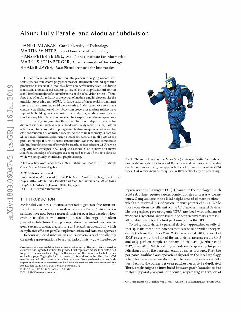
1 INTRODUCTIONMesh subdivision is a ubiquitous method to generate free-form sur-faces from a coarse control mesh, as shown in Figure 1. Subdivisionsurfaces have now been a research topic for over four decades. How-ever, their e�cient evaluation still poses a challenge on modernparallel architectures. During computation, the control mesh under-goes a series of averaging, spli�ing and relaxation operations, whichcomplicates e�cient parallel implementation and data management.

In contrast, serial subdivision implementations traditionally relyon mesh representations based on linked lists, e.g., winged-edge

Permission to make digital or hard copies of all or part of this work for personal orclassroom use is granted without fee provided that copies are not made or distributedfor pro�t or commercial advantage and that copies bear this notice and the full citationon the �rst page. Copyrights for components of this work owned by others than ACMmust be honored. Abstracting with credit is permi�ed. To copy otherwise, or republish,to post on servers or to redistribute to lists, requires prior speci�c permission and/or afee. Request permissions from [email protected].© 2016 ACM. 0730-0301/2016/1-ART1 $15.00DOI: 10.1145/nnnnnnn.nnnnnnn

Fig. 1. The control mesh of the ArmorGuy (courtesy of DigitalFish) subdivi-sion model consists of 9k faces and 10k vertices and features a considerablenumber of creases. Using our approach, the refined mesh at level six (35Mfaces, 35M vertices) can be computed in 40ms without any preprocessing.

representations (Baumgart 1972). Changes to the topology in sucha data structure requires careful pointer updates to preserve consis-tency. Computations in the local neighborhood of mesh vertices—which are essential in subdivision—require pointer chasing. Whilethose operations are e�cient on the CPU, modern parallel devices,like the graphics processing unit (GPU), are faced with unbalancedworkloads, synchronization issues, and sca�ered memory accesses—all of which signi�cantly hurt performance on the GPU.

To bring subdivision to parallel devices, approaches usually ei-ther split the mesh into patches that can be subdivided indepen-dently (Bolz and Schroder 2002, 2003; Patney et al. 2009; Shiue et al.2005) or carry out the bulk of the subdivision process on the CPUand only perform simple operations on the GPU (Nießner et al.2012; Pixar 2018). While spli�ing a mesh seems appealing for paral-lelization at �rst, the approach entails a series of issues. First, theper-patch workload and operations depend on the local topology,which leads to execution divergence between the executing enti-ties. Second, the border between patches needs to be duplicated.�ird, cracks might be introduced between patch boundaries dueto �oating point problems. And fourth, re-patching and workload

ACM Transactions on Graphics, Vol. 1, No. 1, Article 1. Publication date: January 2016.

arX

iv:1

809.

0604

7v3

[cs

.GR

] 1

6 Ja

n 20

19

1:2 • Daniel Mlakar, Martin Winter, Hans-Peter Seidel, Markus Steinberger, and Rhaleb Zayer

distribution might be required as the model gets subdivided recur-sively.

�e alternative—using the CPU to precompute subdivision tablesand only mixing coarse mesh vertices on the GPU—seems an idealsolution for parallel rendering of animated meshes. However, theydo not solve the challenge of parallelization of the subdivision pro-cess, but rather build on the fact that serial preprocessing—whichmay take three orders of magnitude longer than the evaluation—cantake place as long as the model has immutable topology. However,if modeling operations are applied to the mesh or new assets areloaded, preprocessing needs to be applied anew.

Due to the inability of performing the complete subdivision pro-cess e�ciently in parallel, di�erent approaches are used for varioususe cases. When uniform subdivision, e.g., for physics simulation, isrequired, patch-based parallelization can be used. During topology-changing modeling operations, only previews of the full subdivisionare shown to provide high performance. A�er modeling is com-pleted, subdivision tables are used for animation. Finally, duringrendering, partial subdivision or patch-based approaches are usedto reduce the workload. As di�erent approaches also lead to slightlydi�erent results, the meshes used for simulation, preview, animation,and rendering may vary at details—a fact bothering many artists.

With Algebra Subdivision, short AlSub, we provide a fully paralleland modular subdivision approach, ensuring not only consistentresults throughout all application scenarios, but also show signif-icant performance improvements for all of them. AlSub recastsmesh subdivision into linear algebra operations and is the �rst fullyGPU-enabled, universally applicable subdivision implementation. Wemake the following contributions:

• We show that with few linear algebra operations optimizedfor mesh-processing, the entire subdivision process can bedescribed in a compact, self-contained manner suitable forexecution on massively parallel devices like the GPU.

• We show that our sparse linear algebra formalization issu�ciently general to describe many existing subdivisionschemes such as

√3, Loop and Catmull-Clark.

• We show that the proposed approach can be easily extendedto support additions to the standard subdivision algorithms,such as sharp and semi sharp creases, displacement map-ping and subdivision of selected regions, e.g., for featureadaptiveness or path tracing.

• We show that our approach is modular such that topolog-ical operations can be separated from evaluation, leadingto an e�cient parallel preprocessing for immuitable topol-ogy followed by single matrix-vector product for positionupdates, e.g., for animation.

• We show that the involved linear algebra operations canbe specialized and optimized for the use case of mesh pro-cessing, leading to highly optimized subdivision kernels.

A�er a brief summary of related work (Section 2), we present themathematical background and details of our approach for Catmull-Clark subdivision (Section 3). �e important steps for Loop and√

3-subdivision are found in the Appendix. We then highlight howlinear algebra operations are translated and optimized for e�cientmesh processing kernels (Section 4). In Section 5, we show that our

implementation outperforms other publicly available productionand research implementations such as OpenSubdiv (Pixar 2018)and the feature adaptive version of Nießner et al. (2012), as well asthe patch-based GPU subdivision by Patney et al. (2009) in theirrespective domains. We are currently integrating our approach intothe open source modeling and rendering tool Blender (2018).

2 RELATED WORKSubdivision bears some similarity to early ideas in surface ��ingin �nite element analysis (Clough and Tocher 1965) and numericalapproximation (Powell and Sabin 1977) and it has been honed forgeometric modeling through the concerted e�ort of several pioneer-ing researchers, e.g., Chaikin (1974), Doo (1978), Doo and Sabin(1978), and Catmull and Clark (1978).

Subdivision meshes are commonly used across various �elds rang-ing from character animation in feature �lm production (DeRoseet al. 1998) to primitive creation for REYES-style rendering (Zhouet al. 2009), and real-time rendering (Tzeng et al. 2010).

Mesh subdivision is a re�nement procedure which requires datastructures capable of providing and updating connectivity infor-mation. Commonly used data structures are o�en variants of thewinged-edge mesh representations (Baumgart 1972), like quad-edge(Guibas and Stol� 1985) or half-edge (Campagna et al. 1998; Lien-hardt 1994). While they are well suited for use in the serial se�ing,parallel implementations su�er from sca�ered memory accesses,which are particularly harmful to performance. Besides, their stor-age cost is a limiting factor on graphics hardware. Compressedalternative formats which were designed for GPU-rendering, liketriangle stripes (Deering 1995; Hoppe 1999), do not o�er completeconnectivity information and are thus not suitable for subdivision.Patch-based GPU subdivision approaches have thus tried to �nde�cient patch data structures for subdivision (Patney et al. 2009;Shiue et al. 2005).

Most recently, a compact sparse matrix mesh representation hasbeen proposed (Zayer et al. 2017), where mesh processing opera-tions can be expressed as sparse linear algebra and parallelized usinglinear algebra kernels. While the principal applicability of parallelmatrix operations to mesh processing tasks has been reported, morecomplex computations have not been a�empted. In the same spirit,the e�ort undertaken by Mueller-Roemer et al. (2017) for volumetricsubdivision a�empts to use boundary operators for boosting perfor-mance on the GPU. While these di�erential forms have been usedearlier (Castillo et al. 2005), their storage cost and redundanciescontinue to limit their practical scope, especially, as data-sets withmillions of elements are now mainstream.

Given the pressing need for high performance subdivision imple-mentations, various vectorization approaches have been proposed.Shiue et al. (2005) divide the mesh into fragments which can besubdivided independently on the GPU, which reduces inter-threadcommunication but introduces redundant data and computations.Moreover, an initial subdivision step has to be done on the CPU.Subdivision tables have been introduced to e�ciently reevaluate there�ned mesh a�er moving control mesh vertices (Bolz and Schroder2002). However, the creation of such tables requires a symbolicsubdivision, whose cost is similar to a full subdivision. Similarly,


AlSub: Fully Parallel and Modular Subdivision • 1:3

the pre-computed eigenstructure of the subdivision matrix can beused for direct evaluation of Catmull-Clark surfaces (Stam 1998).

To avoid the cost induced by exact subdivision approaches, ap-proximation schemes have been introduced. Peters (2000) proposedan algorithm that transforms the quadrilaterals of a mesh into bicu-bic Nurbs patches. While the resulting surface is tangent continuouseverywhere, the algorithm imposes restricting requirements on themesh. �e approach of Loop and Schaefer (2008) approximates theCatmull-Clark subdivision surface in regular regions using bicu-bic patches. Irregular faces still require additional computations.Approximations like the aforementioned are fast to evaluate, butalong the way, desirable subdivision properties get lost and visualquality deteriorates. While regular faces can be rendered e�cientlyby exploiting the bicubic representation using hardware tessella-tion, irregular regions require recursive subdivision to reduce visualerrors (Nießner et al. 2012). Schafer et al. (2015) took the idea onestep further and enabled di�erent subdivision depths for irregularvertices in a mesh. Brainerd et al. (2016) improved upon these re-sults by introducing subdivision plans. Beyond classical subdivision,several extensions have been proposed to allow for meshes withboundary (Nasri 1987), sharp creases (DeRose et al. 1998), featurebased adaptivity (Nießner et al. 2012), or displacement mapping(Cook 1984; Nießner and Loop 2013).

Our approach avoids the aforementioned shortcomings and re-quires neither CPU preprocessing nor expensive mesh data struc-tures. At the top level, it can be formalized mathematically in theconcise language of linear algebra and hence the ensuing algorithmsare easy to understand and modify without knowledge of the under-lying numerical kernels. �is level also reveals the modular natureof our approach through which it can be adapted for various usecases. At the lower level, our formalization discloses numericalpa�erns across subdivision steps through which we streamline theassociated kernels and increase performance.

3 SPARSE LINEAR ALGEBRA SUBDIVISIONGiven the generality and popularity of the Catmull-Clark subdivi-sion scheme, we will use it to walk through the algorithmic devel-opment of our method. In Appendix A and B, we brie�y show howthe same ideas apply to Loop and

√3 subdivision.

3.1 Classical Formulation�e Catmull-Clark Subdivision scheme o�ers a generalization ofbicubic patches to the irregular mesh se�ing (Catmull and Clark1978). It can be applied to polygonal faces of arbitrary order andalways produces quadrilaterals regardless of the input. Figure 2outlines the four steps of a Catmull-Clark subdivision iteration:

1. Face-point calculation: For an arbitrary polygonal face i oforder ci , the position of face-point fi is set to the barycenter of thepolygon

fi =1ci

ci∑j=1

pj (1)

where pj are the face vertices.

Fig. 2. The Catmull-Clark scheme inserts face-points (le�), edge-points(center), and creates new faces by connecting face-points, edge-points andthe original central point whose location is updated in a smoothing step(right).

2. Edge-point calculation: For each edge pkpl , a new edge-pointis introduced as the average of the endpoints pk and pl and theface-points fr and fs corresponding to the two faces bordering theedge:

ek,l =14 (pk + pl + fr + fs ) . (2)

3. Vertex update: To produce smooth results, the original vertexlocation has to be updated using a linear combination of its old posi-tion, the edge-mid-points of all incident edges and the surroundingface-points

S(pi ) =1ni

©«(ni − 3)pi +1ni

ni∑j=1

fj +2ni

ni∑j=1

12

(pi + pj

)ª®¬ , (3)

where ni is the vertex’s valence, fj are the face-points on adjacentfaces and pj the vertices in the 1-ring neighborhood of pi .

4. Topology re�nement: New edges are inserted that connect theface-point to the face’s edge-points, spli�ing each face of order cinto as many quadrilaterals.

Boundaries: Catmull-Clark subdivision can also be used on mesheswith boundary. Edge-points on boundary edges are placed on theedges’ mid-points. Boundary vertex positions pi are only in�uencedby adjacent boundary vertices

S(pi ) =34pi +

18 (pi−1 + pi+1). (4)

3.2 Linear Algebra FormulationTo derive our linear algebra formulations we use the sparse meshmatrixM (Zayer et al. 2017) as mesh representation. Each columninM corresponds to a face. Row indices of non-zero entries in acolumn correspond to the face’s vertices and the values re�ect thecyclic order of the vertex in the face. �roughout this exposition,we will extend and make use of the action map notation (Zayer et al.2017). �e action map notation is used to express alterations of theclassical behavior of sparse matrix-vector multiplication (SpMV)and sparse matrix-matrix multiplication (SpGEMM), replacing thecore multiplication with alternative operations. In this way, compactformulations of a sequence of operations are possible. Additionally,they also hint at e�cient implementations as the matrix algebracaptures data movement, while action maps capture the actual oper-ations to be carried out. We will revisit these facts when discussing



an e�cient implementation. We explain the action map notationswhere they �rst appear in the following derivation.

Face-point calculation: To compute the barycenters, face orderscan be obtained using an action mapped SpMV

c = MT 1val→1

; (5)

where 1 is a vector of ones spanning the range of the faces. �emapping below the multiplication indicates that the non-zero valuesofMT will be replaced by a 1 during multiplication. �is simplyyields the number of vertices of each face.

�e face-points can then be obtained using the mapped SpMV

f = MT Pvali,∗→ 1

ci

, (6)

where P is the array of all vertex coordinates. In this case, the entriesread from the matrix are used as indices into a one dimensional map.Every non-zero value vali,∗ inMT (i, ∗) is mapped to the reciprocalof the order of face i .

For a quadrilateral mesh, the SpMV simpli�es to

f = MT Pval→ 1

4

. (7)

Edge-point calculation: �e computation of edge points requiresassigning unique indices to mesh edges. Such an enumeration canbe obtained from the upper (or lower) triangular part of the ad-jacency matrix associated with the undirected graph of the mesh.With standard sparse matrix machinery this matrix can be created,for instance, by �rst computing the adjacency matrix of the orientedmesh graph and then summing it with its transpose, to account formeshes with boundaries. In view of our high performance goals,this is not a viable approach since it requires additional data cre-ation (transpose), and more importantly, matrix assembly which isnotoriously challenging on parallel platforms.

With action maps this can be conveniently encoded as

E = MMT

{Qc+Qc−1c }[λ]

. (8)

For the computation of E, the two circulant matrices Qc and itspower Qc−1

c , where c is the face order, are combined to capture thecounterclockwise and clockwise orientation inside a given face. Inthis context, action maps in SpGEMM are small matrices. When-ever a collision between entries of two matrices occurs during theSpGEMM, the non-zero values are used as indices into the map. �emap value is then used as a result of the collision (instead of theproduct of the two values). �erefore, entries in the result matrix ofthe mapped SpGEMM are a sum of map values.

For quads, Q4 captures the CCW and Q34 the CW adjacency.

Q4 =

1 2 3 4

1 0 1 0 02 0 0 1 03 0 0 0 14 1 0 0 0

, Q34 =

1 2 3 4

1 0 0 0 12 1 0 0 03 0 1 0 04 0 0 1 0

; (9)

�ese maps do not have to be created explicitly, as their entries canbe computed on demand. �is is particularly useful, when the face

types vary within a mesh:

Qrc (i, j) =

{1 i f j = ((i + r − 1) mod c) + 10 else

(10)

We extended the original action map notation by functions, λ inEquation 8, which are called each time a collision between elementsM(i,k) andMT (k, j) happens. It performs the map lookup and,depending on the map value, computes the result of a collision:

λ(i, j) = Q(i, j) (11)If the map entry is non-zero, the vertices pi and pj are connectedto each other within a face k . Unique indices for edges can easilybe generated by enumerating the non-zeros in the upper triangularpart of the matrix E.

To complete the computation of edge-points, faces adjacent to agiven edge are required. For this purpose, a secondary matrix F canbe used. �is matrix has the same sparsity pa�ern as the adjacencymatrix of the oriented graph of the mesh but each non-zero entryi, j stores the index of the face containing the edge pipj . It can besimilarly constructed by matrix multiplication such that wheneverthe action map returns a non-zero for a collision between elementsM(i,k) andMT (k, j), the face index k is stored in F (i, j).

F =MMT{Qc }[γ ]

(12)

with the function

γ (i, j,k) ={k i f Qc = 10 else

(13)

Hence, for each edge pipj in the mesh, its unique edge index isknown from E and the two adjacent faces are F (i, j) and F (j, i). �eedge-point position can then be computed.

Vertex update: �e position update in Equation 3 can be conve-niently rewri�en as

S(pi ) =(1 − 2

ni

)pi︸︷︷︸

s1

+1n2i

ni∑j=1

pj︸︷︷︸s2

+1n2i

ni∑j=1

fj︸︷︷︸s3

, (14)

such that the update can be split into three summands. Vertexvalencies can be obtained globally as the vector

n = M1val→1

. (15)

s1 involves only the original position and can be calculated in thecustomary ways.

�e second summand, s2, sums the 1-ring neighborhood of thevertex. �is is done using the matrix F , which has the same sparsitypa�ern as the vertex-vertex adjacency matrix without diagonal, inthe mapped SpMV

s2 = FPvali,∗→ 1

n2i

. (16)

�e last term sums the face-points on faces adjacent to the vertexand is computed via

s3 = Mfvali,∗→ 1

n2i

. (17)



Fig. 3. The core steps of one iteration of our Catmull-Clark subdivision aresplit into a build step, which is concerned with the topological operations,and an evaluation step, which receives information from the build step andthe base mesh vertices.

Topology re�nement: A new face consists of one (updated) vertexof the parent, its face-point and two edge-points. To capture aface in a mesh matrixM, a column representing the polygon hasto be added to the matrix. �e non-zero locations in each newcolumn correspond to the referenced vertices. �us, for creatingthe topology of the subdivided mesh, the computed vertices mustbe referenced accordingly andM of the re�ned mesh matrix has tobe assembled.

A columnM(∗, r ) in the control mesh matrix is replaced by crcolumns in the re�ned mesh matrix where cr is the order of theface. �e indices of the original vertices are already known; theindex of the face-point on fr is |v | + r , where |v | is the number ofmesh vertices. �e indices of the two edge-points can be determinedby fetching the edges’ indices from E and incrementing them by|v | + | f |, where | f | is the number of mesh faces. Performing thesesteps for all new faces yieldsM for the re�ned mesh.

�e combination of all steps mentioned above is outlined in Fig-ure 3. As can be seen, one iteration can be split into a build and aneval step. �e build step takes the current mesh matrix and gener-ates F , E and mesh matrix of the subdivided mesh. In this way, alltopology related operations are carried out by the build step. �eeval step, receives the matrices F and E as well as the mesh matrixand vertex positions from the last iteration. It then carries out themapped SpMVs to generate the new vertex locations.

Boundaries: In practice, meshes o�en feature boundaries, whichneed to be treated using specialized subdivision rules. AlSub handlesboundary meshes in a build and repair fashion. First, the re�nedvertex data is computed as usual. In a subsequent step, boundaryvertices can be conveniently identi�ed from E as entries which havea value of 1, and are repaired in parallel according to Equation4. Edge-points on edges connecting external vertices are set tothe edge-mid points. �eir indices can again be obtained from theenumeration of the non-zeros in the upper triangular part of E.Adding boundaries to our approach essentially forms an additionalstep a�er the default evaluation, as shown in Figure 4.

3.3 CreasesSharp and semi-sharp creases have become indispensable in subdi-vision surface modeling to describe piecewise smooth and tightlycurved surfaces (DeRose et al. 1998), cf. Figure 5. Creases are edges

Fig. 4. Boundary evaluation is captured by our approach as a simple addi-tional step a�er evaluation, and can be seen as a module appended to thestandard evaluation.

Fig. 5. Our approach naturally supports extensions, such as semi-sharp andinfinitely sharp creases, as shown here on a cube.

that are tagged by a (not necessarily) integer sharpness value andupdated according to a special set of rules during subdivision. Asthe general computation of creases is beyond the scope of this paperwe refer the reader to DeRose et al. (1998) for a detailed descrip-tion, while we only present their treatment as sparse matrix linearalgebra.

To support creases, we use a sparse symmetric crease matrix Cof size |v | × |v |. �e entry C(i, j) = σi j holds the sharpness valueof the crease between vertices i and j. To calculate the position ofcrease vertices and edge points, the crease valency k, i.e., numberof creases incident to a crease vertex

k = C1val→1

(18)

and the vertex sharpness s, i.e., average over all incident creasesharpnesses

s = C1vali, j→

vali, jki

(19)

need to be determined, which we complete using the same SpMVwith two di�erent maps. With the computed vectors k and s andthe already available adjacency information in E, we correct creasevertices in parallel using the rules provided by DeRose et al. (1998).A�er each iteration of subdivision a new crease matrix is created,that holds the updated sharpness values for the subdivided creases.�is crease inheritance is performed in two steps: (1) �e sparsitypa�ern is determined by updating crease values according to avariation of Chaikin’s edge subdivision algorithm (Chaikin 1974)that accounts for decreasing sharpness values (DeRose et al. 1998)



Fig. 6. Creases are modeled as a single sparse crease matrix in our approach,which is updated each iteration. During evaluation creases simply overwritethe vertex positions from the previous subdivision step.

σi j = max{ 14

(σi + 3σj

)− 1, 0} (20)

σjk = max{ 14

(3σj + σk

)− 1, 0} (21)

where σi , σj and σk are sharpness values of three adjacent parentcreases i , j and k . σi j and σjk are the sharpness values of the twochild creases of j . To allocate the memory for the new crease matrix,the number of resulting non-zero sharpnesses in each of it’s columnsis counted. (2) �e inherited crease matrix is subsequently �lledwith the remaining non-zero sharpness values. A similar routineas in the �rst step is used which now �lls in the updated non-zerocrease values and their indices. If all crease sharpnesses decreasedto zero, the subsequent subdivision steps are carried out as for asmooth mesh.

�e addition of creases to the evaluation process is outlined inFigure 6. �e core of the subdivision process simply remains thesame; the crease matrix is created additionally in every subdivisioniteration. During evaluation, vertices in�uenced by a crease arereevaluated and overwrite the output vertices.

3.4 Selective and Feature Adaptive Subdivision�e machinery of linear algebra cannot only be used to describeuniform subdivision, but also selective processing, which is inter-esting for hardware supported rendering (Nießner et al. 2012; Pixar2018) and spatially coherent path- and ray-tracing. As example,consider feature adaptive subdivision. In a quadrilateral mesh, faceswith a consistent vertex valence of four can also be represented asbicubic patches and their limit surface can be evaluated directly.�us, for e�ciency reasons, one may want to only recursively sub-divide around vertices with a valence di�erent from four—aroundextraordinary vertices.

Using our scheme, extraordinary vertices are easily identi�edfrom Equation 15, i.e., where the valency is , 4. To identify theregions around the extraordinary vertices, we start with a vectorx0 spanning the number of vertices. x0 is 0 everywhere except forextraordinary vertices, where it is 1. To determine the surroundingfaces, we propagate this information with the mesh matrixM.

First, the neighboring faces are determined as the non-zeros ofthe vector

qi =MT xi (22)

Fig. 7. Selective or feature adaptive subdivision is modeled by the extractionmatrices Xi and Xi , which are generated by identifying the surrounding ofselected vertices. These matrices are applied toM and the vertex data toreduce the subsequent operations to the extracted regions.

and their vertices can be revealed as the non-zero entries resultingfrom the product

xi+1 =Mqi. (23)

�is also shows that the adjacency matrix can be obtained from themapped mesh matrix product and that the power of the adjacencymatrix re�ects the neighborhood order around a vertex.

Using the information from above, we construct the matrix Xi ,which has columns equal to the number of vertices in the inputmesh and rows equal to the number of vertices that are selected forsubdivision. �e entries of Xi correspond to an identity matrix withdeleted rows due to xi+1. �e extraction of the vertex data is thenperformed by the SpMV

P′i = XiPi. (24)

To extract the mesh topology, the matrix Xi—analogue to Xi—iscreated from the information acquired in the propagation step. Xihas rows equal to the number of faces in the original mesh andcolumns equal to the number of faces in the extracted mesh. Xican again be created from the identity matrix by, in contrast to Xi ,deleting columns corresponding to faces that should be disregardedduring extraction. �is information is readily available in qi. �eextracted mesh matrix is then determined via

M ′ = XiMXi (25)

Selective subdivision can be seen as a module added before themajor subdivision step, as shown in Figure 7.

3.5 Other e�ectsNote that displacement mapping and hierarchical edits (Forsey andBartels 1988) are also straight forward in our approach, as we haveaccess to the vertex data a�er each iteration and can arbitrarilymodify it. An example displacement and texture mapped subdivisionmodel can be seen in Figure 8.

3.6 Modes of OperationAs already hinted in the previous sections, AlSub is a modularsystem which allows for dynamic adaption to the requirements ofdi�erent applications. However, we distinguish two main categories:dynamic and static topology of the control mesh.



Fig. 8. AlSub is capable of subdividing a coarse control mesh (top, le�)instantaneously to a dense and smooth refined mesh (top, right). Dis-placement (bo�om, le�) and texture (bo�om, right) mapping are possiblenaturally without any additional e�ort.

Dynamic topology. Dynamic topology is ubiquitous in 3D mod-eling and CAD applications during the content creation process.Faces, vertices and edges are frequently added, modi�ed and re-moved which poses a great challenge to many existing approachesthat rely on expensive preprocessing, as it has to be repeated onevery topological update. �is fact has led to the use of di�erent sub-division approaches for model preview and production renderingcausing discrepancies between the two images. Due to the e�ciencyof our complete approach, we can avoid any preprocessing and al-ternate between what we call build steps and eval steps, computingone complete subdivision step before the next. As additional datalike Fi and Ei are only required for one step, memory requirementsare relatively low in our approach.

Static topology. Static topology is common, e.g., in productionrendering applications, where only vertex a�ributes, e.g. positions,change over time but the mesh connectivity is invariant. Subdivisionalgorithms make heavy use of adjacency information. �e fact thatthis information can be prepared upfront and does not have to bere-computed every frame, reduces the overall production time. InAlSub, all computations dealing with mesh connectivity are factoredinto a build step, that is executed only once before the mesh issubdivided many times, i.e., generating all Fi , Ei and Mi+1 (as wellas Xi and Ci in case of selective subdivision and creases). Onlyin the evaluation step, we process the right side of all modules, asvisualized in the top row of Figure 9.

Single SpMV evaluation. Given that each iteration of the evalua-tion is a sequence of mapped SpMVs, it is also possible to capturethe entire sequence in a single sparse matrix Ri : Ri captures theevaluation of a single subdivision step from level i to level i + 1 .Each column in Ri corresponds to a vertex at subdivision level i andeach row corresponds to one re�ned vertex at level i + 1. A singleiteration of subdivision of vertex data can then be done using theSpMV

Pi+1 = RiPi. (26)Building these re�nement matrices Ri is simple: instead of calcu-lating the re�ned vertices directly as would usually be done in theevaluation step, the weights are distributed into the matrix. We do

Fig. 9. If the topology of the mesh is static only the right-hand side of themodules has to be processed as shown here for adaptive subdivision of aclosed mesh (no boundary handling) with creases, using the iterative eval(top) or the single SpMV eval (bo�om).

this in a two stage approach, where we �rst determine the numberof non-zero entries in each row and in the second stage rows arepopulated with indices and weights.

�e entire evaluation from the �rst level to a speci�c level i canbe wri�en as a sequence of matrix vector products as follows:

Pi = Ri−1Ri−2 . . .R1R0P0 = RP0. (27)

As all matrices involved in Equation 27 are independent of theactual vertex data and therefore only depend on the mesh topologyand features such as creases, the subdivision matrix R can be com-puted in the build step. �at means the whole evaluation step, boilsdown to a single SpMV, regardless of the subdivision depth as shownin Figure 9, bo�om row. �is enables optimization techniques forSpMV kernels to be applied to the evaluation step.

4 OPTIMIZATION OF ALGEBRAIC OPERATIONS�e higher level formalization discussed in Section 3 can be eas-ily implemented by minor adjustment to standard sparse matrixalgebra kernels. However, the compact action map notation hintsthat further specialized and optimized implementations of theseoperations are possible. Using the knowledge about the structure ofthe underlying matrices, we exploit the particular computationalpa�erns of these operations and streamline them through e�cientand highly optimized GPU kernels.

4.1 Reduced Mesh MatrixWe use the Compressed Sparse Column (CSC) matrix format, whichis comprised of three arrays. �e �rst two hold row indices andvalues of non-zero entries. �e column pointer contains an index tothe start of each column in the �rst two arrays (Saad 1994). If eachcolumn inM has the same number of non-zero entries, e.g. quad ortriangle mesh, the column pointer can be omi�ed. Reordering therow index-value pairs ofM according to the values in each columnalso renders the value array unnecessary, because the cyclic orderof vertices in a face is then implicitly given by the order of theirappearance in the row indices array. �e memory requirement of



the reduced mesh matrix is therefore equal to that of a face table ofthe mesh.

As Loop and√

3 work on triangle meshes and Catmull-Clark onlyproduces quadrilaterals, we apply this optimization to all our kernels,using general kernels only for the �rst Catmull-Clark subdivisionstep. In this way, we cut down data creation, memory consumptionand memory accesses.

4.2 Implicit mapped sparse matrix-matrix multiplicationMapped multiplications of the form

A =MMT{Q }[α ]

(28)

are extensively used in our mathematical formalization for cap-turing various connectivity information. Despite the steady im-provement of SpGEMM implementations, their cost is still relativelyhigh. �erefore, it is worthwhile to avoid explicit multiplication ifpossible.

A close examination of what happens during multiplications as inEquation 28 reveals that the result can be directly created fromM.In the computation ofMMT , each row ri =M(i, ∗) is multipliedwith each column c j =MT (∗, j). Both vectors, ri and c j , encode onevertex each and have non-zero entries in the locations correspondingto their adjacent faces. A collision (and with that an invocation ofα ) between two entriesM(i,k) andMT (k, j) happens if both arenon-zero, meaning that vertices i and j share a face k . Clearly,vertices not part of the same face will never induce a collision andtherefore never produce a non-zero entry in the result. Conversely,each non-zero entry is produced by two vertices sharing a face.

�e above �ndings allow us to restructure the computation asfollows: We parallelize over the columns ofM, i.e., the indices ofvertices that form a face. All mapped multiplications that producea non-zero result happen within the same column ofM. Simplyevaluating α for all pairs of vertices of such a column leads to thedesired result. However, as Q and thus α o�en contain many zeroelements, this approach would still lead to wasted computations.�us, instead of using Q to lookup the results for pairs, we use itto guide data loading instead. For a speci�c vertex i , we �nd thoseentries in Q that result in non-zero entries, i.e., the vertex o�setsin the face that result in non-zero results, and directly load thosevalues and evaluate α . In this way, we only load and invoke α forthose pairs of vertices that actually contribute to the output.

Before the actual multiplication can be carried out as describedabove, the number of non-zeros of the result needs to be determined,to allocate the arrays for the output matrix. To this end, we completea symbolic pass, similar to general SpGEMM implementations. Inparallel for each entry of M, we determine the number of localper-face non-zero α invocations for the vertex by counting thenon-zeros in the map row corresponding to the vertex’s position.We atomically accumulate the global number of non-zero for eachvertex in an array, which then corresponds to the number of non-zero entries in the vertex’s column of the result. A simple parallelscan (cumulative sum) over that array gives the column pointer andthe number of non-zeros of the resulting matrix. It is worth notingthat this step can be skipped if each row of the map has the samenumber of non-zero entries zri = zr . �en the number of non-zero

values of the vertex’s column in the result is independent of itsposition in the cyclic order of adjacent faces. �us, the invocationson each vertex can be directly calculated as a multiple of the vertexorder zrn.

4.3 Specialized SpMVsCertain pa�erns in the mapped SpMVs of the higher level formula-tions can be transformed to speci�cally tailored and more e�cientGPU kernels.

Direct mapped SpMV. In the mapped SpMV for CSC matrices,multiple threads collaborate to calculate a single element of theresult vector. Parallelization is done over the elements of the vector.A thread reads a single entry of the input vector and multiplies itwith the mapped non-zero elements of the corresponding column.�ese intermediate products are directly accumulated in the resultvector using an atomic addition operation to avoid race conditions.We found that this execution pa�ern is more e�cient than an explicitmatrix transpose to avoid atomic operations.

Transpose mapped SpMV. Due to using CSC matrices, the trans-pose mapped SpMV can be parallelized easily without an explicittransposition. We use a single thread per output element, whicheliminates the need for atomic operations. Each thread iterates overthe non-zero elements of its column, uses the map to substitutethem and multiplies each mapped value with the correspondingvector element. �is means that in contrast to the direct mappedSpMV, each thread reads multiple elements from the input vector.

Specializations. We distinguish between matrix, vector and map-based optimizations. Depending on the input parameters to themapped SpMVs, we apply all matching optimization steps to producemore e�cient GPU kernels.

If the input matrix is in reduced form, every column has the samenumber of non-zeros, which renders the column pointer obsolete.�is lets us unroll the loop over each column which eliminates costlyconditional jump instructions. Value arrays can also be omi�ed,because row indices in each column are sorted to re�ect the cyclicorder of the face. In both SpMV versions each thread works on onecolumn of the matrix. If the row indices are 16 Byte aligned, e.g.,mesh matrix of a quad mesh, a single vectorized load is used forfour row indices, which increases memory performance.

Many of our operations involve multiplication of the mesh matrixwith a prede�ned input vector, e.g., a vector of ones. In this casethe reads of vector elements is obsolete and can be omi�ed, asspecialized kernels for that speci�c input vector can be generated.In many cases a vector of positions is used in a mapped SpMVwith the mesh matrix. As every input position consists of multiplecomponents the number of threads can be increased such that themultiplication is carried out on a per-component level. Without lossof generality, consider the case of averaging the vertex positionsfor each face, e.g., when calculating face-points in the Catmull-Clark scheme. Each position consists of four components and eachcolumn inM has four non-zero entries. In this case an SpMV kernelis launched with 16 threads per face, each responsible for a singlecomponent of one vertex position. Each group of 16 consecutivethreads then calculates the mapped multiplication of a single column.



As each output component depends on intermediate products offour vertices, e�cient SIMD level communication primitives (shu�einstructions on NVIDIA hardware) are used to combine the results.�e result is then wri�en by a single thread to eliminate the needfor atomics.

Furthermore, we exploit properties of the map to optimize SpMVkernels. If the map is a constant function, the value of the map cansimply reside in shared or constant memory or even in a register toeliminate frequent map lookups. In the non-transposed case, mapsthat are constant per column can be handled similarly.

Single SpMV evaluation. In the adaptive Catmull-Clark imple-mentation we use a single SpMV to subdivide vertex-data from thecontrol mesh to some prede�ned level. As the matrix captures thecombination of multiple mapped SpMVs, there is usually no com-mon structure to exploit. However, as the resulting matrix R is usedfor a single SpMV, we store it in CSR format for a more e�cientrow access. Furthermore, we pad the row indices and value arrays,such that each row is 16 Byte aligned, to enable vectorized loadsindependent of the row length. For the same reason we also pad thevertex-data vector. For evaluation, we assign eight non-zeros to asingle thread which performs the multiplication with eight paddedentries in the vertex array, i.e., 32 values. �en, we use SIMD levelcommunication primitives to merge results that correspond to thesame row spread across multiple threads. Finally, we collect data inon-chip memory �rst, to perform e�cient writes to global memory.As every thread needs to know which row its entries belong to, wecompute this assignment explicitly beforehand. As the matrix isstatic during consecutive evaluations, we compute this informationalready in the build step.

4.4 FusionKernel fusion is an important paradigm in parallel computing, toreduce kernel launch overheads and costly memory transactions.Whenever two operations in the high-level linear algebra formu-lation require the same input vectors and the number of threadsrequired for both computations agree, the two kernels are merged,such that data does not have to be loaded multiple times. For exam-ple in the crease module, the crease valency and vertex sharpness(Equations 18 and 19 respectively) are computed. Both computa-tions involve the same le� and right operands and only di�er in themap, so these two mapped SpMVs are merged into a single kernelthat computes both. Similarly, when the output of a kernel is theinput to the subsequent one, data does not have to go through globalmemory from the �rst to the second kernel but can directly be usedif the kernels are merged. If data causing the dependency is notused in any subsequent computation, the store to global memory isomi�ed. Considering the crease example again, the crease valencycomputed in the �rst mapped SpMV is subsequently used as a mapin the computation of the vertex sharpness. As C is symmetric wecan parallelize over its columns j , compute kj and use it immediatelya�erwards to calculate sj .

4.5 Mesh reorderingFast mesh querying is key to any e�cient, high performance sub-division implementation. While this may be su�cient in theory,

Fig. 10. Evolution of the mesh matrixM of the original and RCM-reorderedAngel model (first and second columns respectively) throughout twoCatmull-Clark iterations. Color-coded geometric layouts of both order-ings are shown on top. The evolution of the respective F matrices is shownin the third and fourth columns.

non-algorithmic factors such as memory access and cache e�ectsare crucial for algorithmic performance in practice. Data layoutin memory directly a�ects access pa�erns and therefore ensuringthe locality of such pa�erns allows us to take advantage of cachingmechanisms. In this way, global reads and writes, which are knownto cause performance deterioration, especially on GPUs, can bereduced.

In our context, this translates to ensuring that primitives whichare topologically close in the mesh, reside close in memory as well.�e layout of a mesh in memory is re�ected in the sparsity pa�ernof the mesh matrix, and locality can be enforced by clustering thenon-zero elements close to the diagonal. Closeness to the diagonalcan be measured in terms of bandwidth (Davis 2006). For bandwidthreduction, the reverse Cuthill McKee (RCM) algorithm is fairly wellknown to produce a comparatively inexpensive, low bandwidthreordering (Cuthill and McKee 1969; George 1971). �e originalRCM only works on square symmetric matrices. To reorder the(usually non-square) mesh matrices, we apply the RCM algorithmto the graph Laplacian of the mesh. �e acquired permutation isapplied to the rows of M and columns are sorted by their �rstnon-zero entry.

As shown in Figure 10, there is no reason to expect mesh creatorsto deliver coherently ordered meshes. Hence, a reordering of theinput can be bene�cial. Due to the way we build Mi+1, the meshordering deteriorates somewhat, as shown for the �rst iteration.While the original vertex indices are copied to the next iteration,a “diagonal-like” line is added for the facepoints, and edge pointsare inserted depending on the connectivity of the original mesh. Ifthe original mesh followed a diagonal pa�ern, the edge points also



correspond to a “diagonal-like” line. Interestingly, the followingsubdivision iteration only adds two “diagonal-like” lines for face andedge points. �us, all iterations show a somewhat tightly alignedsparsity pa�ern. �e same can be observed for E and F , which bothshow a similar pa�ern, with F being displayed in Figure 10.

5 RESULTSWe evaluate two variants of AlSub: formulating the algorithms inthe language of sparse matrix algebra (AlSub pure) as described inSection 3 and a version using the optimized kernels (AlSub opt.)as described in Section 4. While there is a reasonable number ofliterature on parallel subdivision, there are hardly any implemen-tations available for comparison. �us, we mainly compare to thecurrent industry standard, OpenSubdiv, which is based on (Nießneret al. 2012). OpenSubdiv splits subdivision into three steps. First, asymbolic subdivision is performed to create re�ned topology, whichis then used in a second step to precompute the stencil tables forvertex evaluation. We summarize these two steps as build. �e sten-cil tables are then used to perform the evaluation of re�ned vertexdata (eval). While OpenSubdiv executes eval on the GPU, build runsentirely on the CPU. To provide a comparison to a complete GPUimplementation, we compare against Patney et al. (2009) .

All tests are performed on an Intel Core i7-7700 with 32GB ofRAM and an Nvidia GTX 1080 Ti. �e provided measurements arethe sum of all kernel timings required for the subdivision, averagedover several runs. �e input models are unaltered and thus havenot been reordered unless speci�cally marked di�erently.

5.1 Catmull-Clark performanceAs test models for Catmull-Clark subdivision we use a variety ofdi�erently sized meshes which are listed in Table 1 with the testedsubdivision level. As AlSub is a modular approach which can adaptto di�erent applications, we distinguish two use cases: “modeling”and “rendering”.

mesh cf cv ni rf rv

Catm

ull-C

lark

threeblock 18 20 5 18k 18kpig 381 389 5 390k 390kmonsterfrog 1.3k 1.3k 4 331k 331kcomplex 1.4k 1.3k 4 346k 346kbigguy 1.5k 1.5k 4 371k 371kArmorGuy 8.6k 10.0k 6 35.2M 35.3Mhat 4.4k 4.4k 6 18.1M 18.1Mcoat 5.6k 5.7k 6 22.8M 22.8Mcupid 29k 29k 2 458k 458kbike 53.9k 54.3k 4 13.4M 13.5Mcar 149.7k 164.9k 4 38.5M 38.7Mdress 2.3k 2.4k 6 9.2M 9.2Mbee 16.9M 8.5M 1 50.8M 50.8Mneptune 4.0M 2.0M 2 48.1M 48.1M

Table 1. Catmull-Clark test meshes: Number of faces cf and vertices cvof the control meshes, as, well as the applied number of iterations ni andfaces rf and vertices rv in the refined mesh.

Modeling. �is speci�c use case is a representative for the classof applications in which the mesh topology changes frequently.Topological changes require re-computation of eventually prepro-cessed data e.g. subdivision tables. Results are given in Figure 12.�e comparison between AlSub pure, AlSub opt., and OpenSubdiv(le�) shows complex meshes. We observe that AlSub opt. is morethan one order of magnitude faster than AlSub pure, highlightingthe gains of our optimizations. AlSub pure is about one order ofmagnitude faster than OpenSubdiv when performing preprocessingand evaluation. �is shows that our complete parallel GPU imple-mentation is signi�cantly faster than the split CPU and GPU buildand eval approach of OpenSubdiv if a topology-changing modelingoperation is carried out. Note that this is not the default use case ofOpenSubdiv which assumes mostly static topology. Nevertheless,this delay might still yield unpleasant behavior during topologychanging modeling operations. Note that the memory requirementsfor the entire subdivision of AlSub opt. are usually signi�cantlybelow OpenSubdiv’s stencil tables. AlSub pure needs signi�cantlymore memory and thus was unable to execute on the very largemeshes Bee and Neptune.

As OpenSubdiv is clearly more focused on e�cient evaluationthan optimizing the whole subdivision pipeline, we also compared tothe GPU-based Catmull-Clark implementation by Patney et al. (Pat-ney et al. 2009), which we con�gured to perform uniform subdivi-sion. We could only test small quad-only models, as their implemen-tation seems to have issues when generating more geometry andfails on meshes with triangles. Nevertheless, as seen in Figure 12(right) AlSub opt. is about 2 − 3× faster than the patch-based im-plementation of Patney et al.. We a�ribute this fact to the highlystreamlined performance of our formulations and optimizations,which show zero redundant work and result in e�cient memorymovements.

Rendering. In contrast to modeling, topology is considered staticin rendering, which is the intended use case of OpenSubdiv. In thiscase, information required during subdivision that only dependson the topology can be precomputed and stored for later use. �eevaluation stage uses this information to subdivide the vertex datain every render frame, e.g., when replaying an animation. Relyingon AlSub’s split into build and eval modules, similar optimizationsare possible in our approach. Figure 13 shows that when spli�ingour approach into these two phases, AlSub opt. achieves nearly oneorder of magnitude performance gain over AlSub pure in both buildand eval. Furthermore, performing the build stage complete onthe GPU, yields signi�cant performance gains over OpenSubdiv’sbuild stage, even when building the matrix R for the single SpMVevaluation (AlSub opt. B&E sSPMV).

Even more important for this use case is that AlSub opt. as wellas AlSub opt. sSpMV also outperform OpenSubdiv in the eval step.Comparing the customary AlSub opt. evaluation to the single SpMVmodule reveals a slight edge of sSPMV. Performance of AlSub opt.decreases below that of OpenSubdiv for the Armor Guy modelwith its high number of creases, for which our approach in itscurrent form performs additional steps to “�x” the geometry. Ascreases are simply incorporated into the subdivision matrix R inthe single SpMV evaluation, it does not su�er from that slowdown.



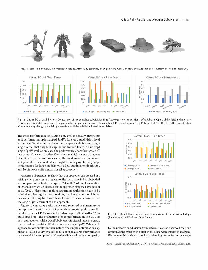
Fig. 11. Selection of evaluation meshes: Neptune, ArmorGuy (courtesy of DigitalFish), Girl, Car, Hat, and Eulaema Bee (courtesy of The Smithsonian).

1E+0

1E+1

1E+2

1E+3

1E+4

1E+5

mill

isec

onds

Catmull-Clark Total Times

AlSub opt. AlSub pure OpenSubdiv

0E+0

1E+3

2E+3

3E+3

4E+3

5E+3

6E+3M

BCatmull-Clark Peak Mem.


0.0

1.0

2.0

3.0

4.0

5.0

6.0

mill

isec

onds

Catmull-Clark Patney et al.

AlSub opt. Patney et al.

Fig. 12. Catmull-Clark subdivision: Comparison of the complete subdivision time (topology + vertex positions) of AlSub and OpenSubdiv (le�) and memoryrequirements (middle). A separate comparison for simpler meshes with the complete GPU-based approach by Patney et al. (right). This is the time it takesa�er a topology changing modeling operation until the subdivided mesh is available.

�e good performance of AlSub’s opt. eval is actually surprising,as it performs multiple mapped SpMVs for every subdivision level,while OpenSubdiv can perform the complete subdivison using asingle kernel that only looks up the subdivision tables. AlSub’s opt.single SpMV evaluation leads the performance chart throughout alltest cases. However, it su�ers from the same high memory usage asOpenSubdiv in the uniform case, as the subdivision matrix, as wellas OpenSubdiv’s stencil tables, might become prohibitively large.Performance for large models with a low subdivision depth (Beeand Neptune) is quite similar for all approaches.

Adaptive Subdivision. To show that our approach can be used in ase�ing where only certain regions of the mesh have to be subdivided,we compare to the feature adaptive Catmull-Clark implementationof OpenSubdiv, which is based on the approach proposed by Nießneret al. (2012). Here, only regions around irregularities have to besubdivided. For regular mesh regions, patches are built which canbe evaluated using hardware tessellation. For evaluation, we usethe Single SpMV variant of our approach.

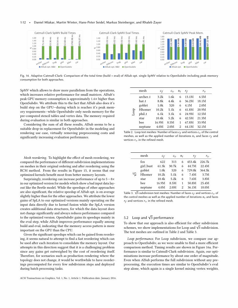
Figure 14 compares performance and required peak memory ofour approaches with those of OpenSubdiv. Again, performing thebuild step on the GPU shows a clear advantage of AlSub with a 17.7×build speed-up. �e evaluation step is performed on the GPU inboth approaches—while OpenSubdiv uses its stencil tables to createthe re�ned vertex-data, AlSub performs a single SpMV. While bothapproaches are similar in their nature, the simple optimizations ap-plied to AlSub’s SpMV evaluation re�ect in an average performanceincrease of 2.3× compared to OpenSubdiv’s eval. When comparing

1E+0

1E+1

1E+2

1E+3

1E+4

1E+5

mill

isec

onds

Catmull-Clark Build Times

AlSub opt. B&E AlSub opt. B&E sSpMVAlSub pure B&E OpenSubdiv

1E+0

1E+1

1E+2

1E+3

mill

isec

onds

Catmull-Clark Eval Times

AlSub opt. B&E AlSub opt. B&E sSpMVAlSub pure B&E OpenSubdiv

Fig. 13. Catmull-Clark subdivision: Comparison of the individual steps(build & eval) of AlSub and OpenSubdiv.

to the uniform subdivision from before, it can be observed that ouroptimizations work even be�er in this case with smaller R matrices.We believe this is due to our load balancing strategies in the single



75.1

6m

s

63.3

6m

s

59.5

4m

s

62.6

8m

s

3790

.98

ms

8976

.07

ms

0.000.200.400.600.801.001.201.401.60

%Catmull-Clark SpMV Build Times

AlSub opt. B&E OpenSubdiv

0.02

ms

0.02

ms

0.02

ms

0.02

ms

0.62

ms

1.61

ms

0.000.200.400.600.801.001.201.40

%

Catmull-Clark SpMV Eval Times

AlSub opt. B&E OpenSubdiv

5.01

MB

4.39

MB

4.09

MB

4.43

MB

250.

91M

B

607.

22M

B

0.000.200.400.600.801.001.201.401.601.80

%

Catmull-Clark SpMV Peak Mem.

AlSub opt. OpenSubdiv

Fig. 14. Adaptive Catmull-Clark: Comparison of the total time (build + eval) of AlSub opt. single SpMV relative to OpenSubdiv including peak memoryconsumption for both approaches.

SpMV which allows to draw more parallelism from the operations,which increases relative performance for small matrices. AlSub’speak GPU memory consumption is approximately 1.6× higher thanOpenSubdiv. We a�ribute this to the fact that AlSub also does it’sbuild step on the GPU—during which is reaches it’s peak mem-ory requirements—while OpenSubdiv only needs memory for thepre-computed stencil tables and vertex data. �e memory requiredduring evaluation is similar in both approaches.

Considering the sum of all these results, AlSub seems to be asuitable drop-in replacement for OpenSubdiv in the modeling andrendering use case, virtually removing preprocessing costs andsigni�cantly increasing evaluation performance.

Mesh reordering. To highlight the e�ect of mesh reordering, wecompared the performance of di�erent subdivision implementationson meshes in their original ordering and a�er reordering using theRCM method. From the results in Figure 15, it seems that ouroptimized kernels bene�t most from be�er memory layouts.

Surprisingly, reordering can increase performance of up to 5− 8×in our optimized version for models which show a bad input data lay-out like the Beetle model. While the speedups of other approachesare also signi�cant, the relative speedup of AlSub opt. is on averageslightly higher than for the other approaches. We a�ribute the lowergains of SpLA to our optimized versions mainly operating on theinput data directly due to kernel fusion while the SpLA versioncreates additional data structures, for which the data layout doesnot change signi�cantly and always reduces performance comparedto the optimized version. OpenSubdiv gains its speedups mainly inthe eval step, while AlSub improves performance equally amongbuild and eval, indicating that the memory access pa�ern is moreimportant on the GPU than the CPU.

Given the signi�cant speedups which can be gained from reorder-ing, it seems natural to a�empt to �nd a fast reordering which canbe used a�er each iteration to consolidate the memory layout. Oura�empts in this direction suggest that it is a challenging problemsince any gains get outweighed by the cost of reordering itself.�erefore, for scenarios such as production rendering where thetopology does not change, it would be worthwhile to have reorder-ings precomputed for every few subdivision steps and deployedduring batch processing tasks.

mesh cf cv ni rf rv

Loop

archer t 3.2k 1.6k 6 13.1M 6.5Mhat t 8.8k 4.4k 6 36.2M 18.1Mgoblet 1.0k 520 6 4.1M 2.0MHhomer 10.2k 5.1k 6 41.8M 20.9Mphil t 6.1k 3.1k 6 24.9M 12.5Mstar 10.4k 5.2k 6 42.5M 21.3Mbee 16.9M 8.5M 1 67.8M 33.9Mneptune 4.0M 2.0M 2 64.1M 32.1M

Table 2. Loop test meshes: Number of faces cf and vertices cv of the controlmeshes, as well as the applied number of iterations ni and faces rf andvertices rv in the refined mesh.

mesh cf cv ni rf rv

√ 3

fox 622 313 6 453.4k 226.7kgirl bust 61.3k 30.7k 6 44.7M 22.4Mgoblet 1.0k 520 6 729.0k 364.5kHhomer 10.2k 5.1k 6 7.4M 3.7Mstar 10.4k 5.2k 6 7.6M 3.8Mbee 16.9M 8.5M 1 50.8M 25.4Mneptune 4.0M 2.0M 2 36.1M 18.0M

Table 3.√

3-subdivision test meshes: Number of faces cf and vertices cv ofthe control meshes as well as the applied number of iterations ni and facesrf and vertices rv in the refined mesh.

5.2 Loop and√

3 performanceTo show that our approach is also e�cient for other subdivisionschemes, we show implementations for Loop and

√3 subdivision.

�e test meshes are outlined in Table 2 and Table 3.

Loop performance. For Loop subdivison, we compare our ap-proach to OpenSubdiv, as we were unable to �nd a more e�cientcomparison method. Timing results are shown in Figure 16a. Per-formance is similar to Catmull-Clark subdivision. Again, our opti-mizations increase performance by about one order of magnitude.Even when AlSub performs the full subdivision without any pre-processing, the execution times are similar to OpenSubdiv’s evalstep alone, which again is a single kernel mixing vertex weights.



0

2

4

6

8

10

Spee

dup

Reordering Build Speedup

AlSub opt. build AlSub pure buildOpenSubdiv build

0123456

Spee

dup

Reordering Eval Speedup

AlSub opt. eval AlSub pure evalOpenSubdiv eval

012345678

Spee

dup

Reordering Total Speedup

AlSub opt. total AlSub pure totalOpenSubdiv total

Fig. 15. Reordering results as relative speed up to the non-reordered meshes over one Catmull-Clark iteration (no postfix) and two iterations (’;2’ postfix).

1E-11E+01E+11E+21E+31E+41E+5

mill

seco

nds

Loop Total Times

AlSub opt. AlSub pureOpenSubdiv - Build OpenSubdiv - Eval

(a) Loop subdivision performance

0.0E+0

5.0E+2

1.0E+3

1.5E+3

2.0E+3

2.5E+3

3.0E+3M

BLoop Peak Mem.


(b) Loop memory requirements.

1E+0

1E+1

1E+2

1E+3

1E+4

1E+5

mill

isec

onds

Sqrt3 Total Times

AlSub opt. AlSub pure OpenMesh

(c)√

3 performance

Fig. 16. Performance comparisons of AlSub’s Loop and√

3 subdivision implementations to OpenSubdiv’s Loop and OpenMesh’s√

3.

�e CPU build times of OpenSubdiv are signi�cantly higher. Whenspli�ing our approach into build and eval and performing singleSpMV optimizations, similar speedups are achieved as before. Toreduce space, we omit that data here. �e memory requirements ofAlSub opt. are again lower than AlSub pure. Interestingly, OpenSub-div shows higher memory requirements than AlSub pure in manycases.√

3 performance. As OpenSubdiv lacks support for this schemeand we are not aware of any GPU implementation of

√3, we compare

AlSub pure, Alsub opt. and OpenMesh in Figure 16c. While it is clear,that a parallel GPU implementation is capable of outperforming aserial CPU approach, it shows the bene�ts of a fully parallelizedsubdivision pipeline. �roughout all experiments, the optimizedAlSub opt. achieved a performance gain of 10× or more comparedto it’s unoptimized counterpart. Especially when starting witha smaller input model, AlSub opt. pulls away further, which wea�ribute mostly due the involved SpGEMM operations which showa certain overhead independent of the input size. �is overhead alsore�ects in the temporary memory requirements, which prohibit verylarge meshes (bee or neptune) to complete with our unoptimizedversion. AlSub opt. handles these cases without trouble.

6 CONCLUSIONIn this paper, we proposed a full �edged treatment of parallel meshsubdivision using linear algebra primitives (AlSub). Our approach ismodular and extensible, suitable for di�erent subdivision schemesand handles additional features, like treatment of mesh boundaries,

creases, and selective subdivision. Unlike traditional approaches,where bookkeeping stalls performance and impedes vectorization,our treatment allows for e�cient parallel implementations. Whilea direct implementation of this formulation already indicates highthroughput, we show a series of optimizations that increase per-formance by another order of magnitude throughout all test cases.�e evaluation shows that our subdivision approach signi�cantlyoutperforms other implementations in scenarios where an inputmesh must be subdivided once (2− 3× faster than patch-based GPUimplementations). Spli�ing the subdivision into preprocessing andevaluation for cases where the topology does not change, makes it adirect competitor to OpenSubdiv. Performing the preprocessing stepon the GPU shows extreme speedups compared to OpenSubdiv’sCPU preprocessing. At the same time, our evaluation step is up to2× faster than OpenSubdiv. While we have shown how to writeand optimize subdivision approaches in a complete sparse-linearalgebra manner, many other types of mesh processing algorithmsare equally suitable to this treatment. We believe a general linearalgebra library for mesh processing would bene�t many domains.Automatically identifying optimization potentials and applying sim-ilar steps as we have proposed in this work may open up the highcompute power of modern GPUs for many geometry processingalgorithms.

REFERENCESBruce G. Baumgart. 1972. Winged Edge Polyhedron Representation. Technical Report.

Stanford, CA, USA.



Je�rey Bolz and Peter Schroder. 2002. Rapid Evaluation of Catmull-Clark SubdivisionSurfaces. In Proceedings of the Seventh International Conference on 3DWeb Technology(Web3D ’02). ACM, New York, NY, USA, 11–17. h�ps://doi.org/10.1145/504502.504505

Je�rey Bolz and Peter Schroder. 2003. Evaluation of Subdivision Surfaces on Pro-grammable Graphics Hardware. (Mar 2003), 4. h�p://ww.multires.caltech.edu/pubs/GPUSubD.pdf

Wade Brainerd, Tim Foley, Manuel Kraemer, Henry Moreton, and Ma�hias Nießner.2016. E�cient GPU Rendering of Subdivision Surfaces Using Adaptive �adtrees.ACM Trans. Graph. 35, 4, Article 113 (July 2016), 12 pages. h�ps://doi.org/10.1145/2897824.2925874

Swen Campagna, Leif Kobbelt, and Hans-Peter Seidel. 1998. Directed edges-A scalablerepresentation for triangle meshes. Journal of Graphics tools 3, 4 (1998), 1–11.

Paul Castillo, Robert Rieben, and Daniel White. 2005. FEMSTER: An Object-orientedClass Library of High-order Discrete Di�erential Forms. ACM Trans. Math. So�w.31, 4 (Dec. 2005), 425–457. h�ps://doi.org/10.1145/1114268.1114269

Edwin Catmull and James Clark. 1978. Recursively generated B-spline surfaces onarbitrary topological meshes. Computer-Aided Design 10, 6 (1978), 350 – 355. h�ps://doi.org/10.1016/0010-4485(78)90110-0

George M. Chaikin. 1974. An algorithm for high speed curve generation. ComputerGraphics and Image Processing 3 (1974), 346–349.

Ray W. Clough and J. L. Tocher. 1965. Finite Element Sti�ness Matrices for Analysisof Plates in Bending. In Proceedings of Conference on Matrix Methods in StructuralMechanics. Wright-Pa�erson A. F. B., Ohio. Air Force Institute of Technology.

Blender Online Community. 2018. Blender 3D Creation Suite. h�ps://www.blender.orgRobert L. Cook. 1984. Shade Trees. SIGGRAPH Comput. Graph. 18, 3 (Jan. 1984), 223–231.

h�ps://doi.org/10.1145/964965.808602Elizabeth Cuthill and James McKee. 1969. Reducing the Bandwidth of Sparse Symmetric

Matrices. In Proceedings of the 1969 24th National Conference (ACM ’69). ACM, NewYork, NY, USA, 157–172. h�ps://doi.org/10.1145/800195.805928

Timothy Davis. 2006. Direct Methods for Sparse Linear Systems. Society for Industrialand Applied Mathematics. h�ps://doi.org/10.1137/1.9780898718881

Michael Deering. 1995. Geometry Compression. In Proceedings of the 22Nd AnnualConference on Computer Graphics and Interactive Techniques (SIGGRAPH ’95). ACM,New York, NY, USA, 13–20. h�ps://doi.org/10.1145/218380.218391

Tony DeRose, Michael Kass, and Tien Truong. 1998. Subdivision Surfaces in CharacterAnimation. In Proceedings of the 25th Annual Conference on Computer Graphics andInteractive Techniques (SIGGRAPH ’98). ACM, New York, NY, USA, 85–94. h�ps://doi.org/10.1145/280814.280826

Daniel Doo. 1978. A subdivision algorithm for smoothing down irregularly shapedpolyhedrons. In Proced. Int’l Conf. Ineractive Techniques in Computer Aided Design.157–165. Bologna, Italy, IEEE Computer Soc.

Daniel Doo and Malcolm Sabin. 1978. Behaviour of Recursive Division Surfaces NearExtraordinary Points. Computer-Aided Design 10 (Sept. 1978), 356–360.

David R. Forsey and Richard H. Bartels. 1988. Hierarchical B-spline Re�nement. InProceedings of the 15th Annual Conference on Computer Graphics and InteractiveTechniques (SIGGRAPH ’88). ACM, New York, NY, USA, 205–212. h�ps://doi.org/10.1145/54852.378512

John A. George. 1971. Computer Implementation of the Finite Element Method. Ph.D.Dissertation. Stanford, CA, USA. AAI7205916.

Leonidas Guibas and Jorge Stol�. 1985. Primitives for the Manipulation of GeneralSubdivisions and the Computation of Voronoi. ACM Trans. Graph. 4, 2 (April 1985),74–123. h�ps://doi.org/10.1145/282918.282923

Hugues Hoppe. 1999. Optimization of Mesh Locality for Transparent Vertex Caching.In Proceedings of the 26th Annual Conference on Computer Graphics and InteractiveTechniques (SIGGRAPH ’99). ACM Press/Addison-Wesley Publishing Co., New York,NY, USA, 269–276. h�ps://doi.org/10.1145/311535.311565

Leif Kobbelt. 2000.√

3-subdivision. In Proceedings of the 27th Annual Conference onComputer Graphics and Interactive Techniques (SIGGRAPH ’00). ACM Press/Addison-Wesley Publishing Co., New York, NY, USA, 103–112. h�ps://doi.org/10.1145/344779.344835

Pascal Lienhardt. 1994. N-dimensional generalized combinatorial maps and cellularquasi-manifolds. International Journal of Computational Geometry & Applications 4,03 (1994), 275–324.

Charles Loop. 1987. Smooth subdivision surfaces based on triangles. (1987).Charles Loop and Sco� Schaefer. 2008. Approximating Catmull-Clark Subdivision

Surfaces with Bicubic Patches. ACM Trans. Graph. 27, 1, Article 8 (March 2008),11 pages. h�ps://doi.org/10.1145/1330511.1330519

Johannes S. Mueller-Roemer, Christian Altenhofen, and Andre Stork. 2017. TernarySparse Matrix Representation for Volumetric Mesh Subdivision and Processing onGPUs. Computer Graphics Forum 36, 5 (2017), 59–69. h�ps://doi.org/10.1111/cgf.13245

Ahmad H. Nasri. 1987. Polyhedral Subdivision Methods for Free-form Surfaces. ACMTrans. Graph. 6, 1 (Jan. 1987), 29–73. h�ps://doi.org/10.1145/27625.27628

Ma�hias Nießner and Charles Loop. 2013. Analytic Displacement Mapping UsingHardware Tessellation. ACM Trans. Graph. 32, 3, Article 26 (July 2013), 9 pages.

h�ps://doi.org/10.1145/2487228.2487234Ma�hias Nießner, Charles Loop, Mark Meyer, and Tony DeRose. 2012. Feature-adaptive

GPU Rendering of Catmull-Clark Subdivision Surfaces. ACM Trans. Graph. 31, 1,Article 6 (Feb. 2012), 11 pages. h�ps://doi.org/10.1145/2077341.2077347

Anjul Patney, Mohamed S. Ebeida, and John D. Owens. 2009. Parallel View-dependentTessellation of Catmull-Clark Subdivision Surfaces. In Proceedings of the Conferenceon High Performance Graphics 2009 (HPG ’09). ACM, New York, NY, USA, 99–108.h�ps://doi.org/10.1145/1572769.1572785

Jorg Peters. 2000. Patching Catmull-Clark Meshes. In Proceedings of the 27th AnnualConference on Computer Graphics and Interactive Techniques (SIGGRAPH ’00). ACMPress/Addison-Wesley Publishing Co., New York, NY, USA, 255–258. h�ps://doi.org/10.1145/344779.344908

Graphics Technologies Pixar. 2018. OpenSubdiv. h�p://graphics.pixar.com/opensubdiv/docs/intro.html

Michael J. D. Powell and Malcolm Sabin. 1977. Piecewise �adratic Approximationson Triangles. ACM Trans. Math. So�w. 3, 4 (Dec. 1977), 316–325. h�ps://doi.org/10.1145/355759.355761

Youcef Saad. 1994. SPARSKIT: A Basic Tool Kit for Sparse Matrix Computations. TechnicalReport. Computer Science Department, University of Minnesota, Minneapolis, MN55455.

Henry Schafer, Jens Raab, Benjamin Keinert, Mark Meyer, Marc Stamminger, andMa�hias Nießner. 2015. Dynamic Feature-adaptive Subdivision. In Proceedings ofthe 19th Symposium on Interactive 3D Graphics and Games (i3D ’15). ACM, New York,NY, USA, 31–38. h�ps://doi.org/10.1145/2699276.2699282

Le-Jeng Shiue, Ian Jones, and Jorg Peters. 2005. A Realtime GPU Subdivision Kernel. InACM SIGGRAPH 2005 Papers (SIGGRAPH ’05). ACM, New York, NY, USA, 1010–1015.h�ps://doi.org/10.1145/1186822.1073304

Jos Stam. 1998. Exact Evaluation of Catmull-Clark Subdivision Surfaces at ArbitraryParameter Values. In Proceedings of the 25th Annual Conference on Computer Graphicsand Interactive Techniques (SIGGRAPH ’98). ACM, New York, NY, USA, 395–404.h�ps://doi.org/10.1145/280814.280945

Stanley Tzeng, Anjul Patney, and John D. Owens. 2010. Task Management for Irregular-parallel Workloads on the GPU. In Proceedings of the Conference on High PerformanceGraphics (HPG ’10). Eurographics Association, Aire-la-Ville, Switzerland, Switzer-land, 29–37. h�p://dl.acm.org/citation.cfm?id=1921479.1921485

Rhaleb Zayer, Markus Steinberger, and Hans-Peter Seidel. 2017. A GPU-AdaptedStructure for Unstructured Grids. Computer Graphics Forum 36, 2 (May 2017),495–507. h�ps://doi.org/10.1111/cgf.13144

Kun Zhou, Qiming Hou, Zhong Ren, Minmin Gong, Xin Sun, and Baining Guo. 2009.RenderAnts: Interactive Reyes Rendering on GPUs. In ACM SIGGRAPH Asia 2009Papers (SIGGRAPH Asia ’09). ACM, New York, NY, USA, Article 155, 11 pages.h�ps://doi.org/10.1145/1661412.1618501

A√

3-SUBDIVISION�e√

3-subdivision scheme is specialized for triangle meshes and isbased on a uniform split operator which introduces a new vertex forevery triangle of the input mesh (Kobbelt 2000). It de�nes a naturalstationary subdivision scheme with stencils of minimum size andmaximum symmetry.

�e subdivision process involves two major steps. �e �rst oneinserts a new vertex fi at the center of every triangle i .

Each new vertex is then connected to the vertices of its mastertriangle and an edge �ip is then applied to the original edges, seeFigure 17. In the second step, the positions of the old vertices areupdated using the following smoothing rule

S(pi ) = (1 − αi )pi +αini

ni∑1pj (29)

where ni is the valence of vertex pi and αn is obtained by analyz-ing the eigen-structure of the subdivision matrix:

αi =4 − 2 cos( 2πni )

9 . (30)

Clearly the topological operations involved in this scheme anticipatean edge-based mesh representation and all the implementations weare aware of rely on the half-edge data structure.


https://doi.org/10.1145/504502.504505

https://doi.org/10.1145/504502.504505

http://ww.multires.caltech.edu/pubs/GPUSubD.pdf

http://ww.multires.caltech.edu/pubs/GPUSubD.pdf

https://doi.org/10.1145/2897824.2925874

https://doi.org/10.1145/2897824.2925874

https://doi.org/10.1145/1114268.1114269

https://doi.org/10.1016/0010-4485(78)90110-0

https://doi.org/10.1016/0010-4485(78)90110-0

https://www.blender.org

https://doi.org/10.1145/964965.808602

https://doi.org/10.1145/800195.805928

https://doi.org/10.1137/1.9780898718881

https://doi.org/10.1145/218380.218391

https://doi.org/10.1145/280814.280826

https://doi.org/10.1145/280814.280826

https://doi.org/10.1145/54852.378512

https://doi.org/10.1145/54852.378512

https://doi.org/10.1145/282918.282923

https://doi.org/10.1145/311535.311565

https://doi.org/10.1145/344779.344835

https://doi.org/10.1145/344779.344835

https://doi.org/10.1145/1330511.1330519

https://doi.org/10.1111/cgf.13245


https://doi.org/10.1145/27625.27628

https://doi.org/10.1145/2487228.2487234

https://doi.org/10.1145/2077341.2077347

https://doi.org/10.1145/1572769.1572785

https://doi.org/10.1145/344779.344908

https://doi.org/10.1145/344779.344908

http://graphics.pixar.com/opensubdiv/docs/intro.html

http://graphics.pixar.com/opensubdiv/docs/intro.html

https://doi.org/10.1145/355759.355761

https://doi.org/10.1145/355759.355761

https://doi.org/10.1145/2699276.2699282

https://doi.org/10.1145/1186822.1073304

https://doi.org/10.1145/280814.280945

http://dl.acm.org/citation.cfm?id=1921479.1921485


https://doi.org/10.1145/1661412.1618501


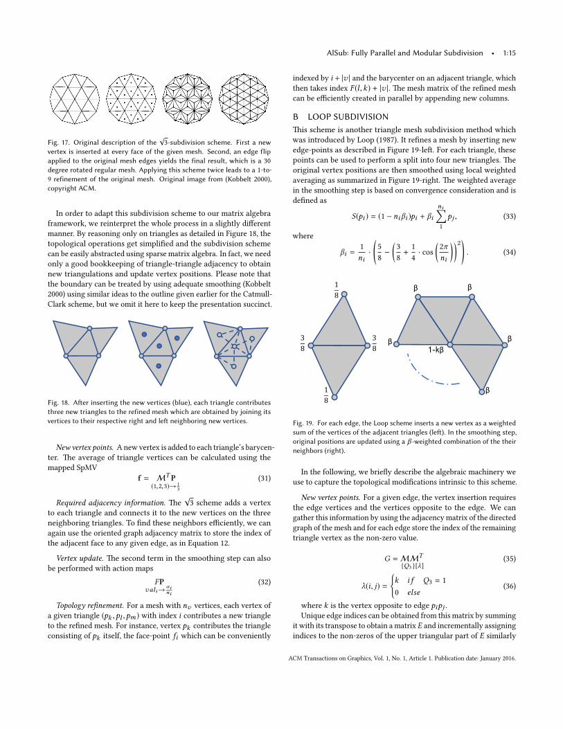
Fig. 17. Original description of the√

3-subdivision scheme. First a newvertex is inserted at every face of the given mesh. Second, an edge flipapplied to the original mesh edges yields the final result, which is a 30degree rotated regular mesh. Applying this scheme twice leads to a 1-to-9 refinement of the original mesh. Original image from (Kobbelt 2000),copyright ACM.

In order to adapt this subdivision scheme to our matrix algebraframework, we reinterpret the whole process in a slightly di�erentmanner. By reasoning only on triangles as detailed in Figure 18, thetopological operations get simpli�ed and the subdivision schemecan be easily abstracted using sparse matrix algebra. In fact, we needonly a good bookkeeping of triangle-triangle adjacency to obtainnew triangulations and update vertex positions. Please note thatthe boundary can be treated by using adequate smoothing (Kobbelt2000) using similar ideas to the outline given earlier for the Catmull-Clark scheme, but we omit it here to keep the presentation succinct.

Fig. 18. A�er inserting the new vertices (blue), each triangle contributesthree new triangles to the refined mesh which are obtained by joining itsvertices to their respective right and le� neighboring new vertices.

New vertex points. A new vertex is added to each triangle’s barycen-ter. �e average of triangle vertices can be calculated using themapped SpMV

f = MT P(1,2,3)→ 1

3

(31)

Required adjacency information. �e√

3 scheme adds a vertexto each triangle and connects it to the new vertices on the threeneighboring triangles. To �nd these neighbors e�ciently, we canagain use the oriented graph adjacency matrix to store the index ofthe adjacent face to any given edge, as in Equation 12.

Vertex update. �e second term in the smoothing step can alsobe performed with action maps

FPvali→ αi

ni

(32)

Topology re�nement. For a mesh with nv vertices, each vertex ofa given triangle (pk ,pl ,pm ) with index i contributes a new triangleto the re�ned mesh. For instance, vertex pk contributes the triangleconsisting of pk itself, the face-point fi which can be conveniently

indexed by i + |v | and the barycenter on an adjacent triangle, whichthen takes index F (l ,k) + |v |. �e mesh matrix of the re�ned meshcan be e�ciently created in parallel by appending new columns.

B LOOP SUBDIVISION�is scheme is another triangle mesh subdivision method whichwas introduced by Loop (1987). It re�nes a mesh by inserting newedge-points as described in Figure 19-le�. For each triangle, thesepoints can be used to perform a split into four new triangles. �eoriginal vertex positions are then smoothed using local weightedaveraging as summarized in Figure 19-right. �e weighted averagein the smoothing step is based on convergence consideration and isde�ned as

S(pi ) = (1 − niβi )pi + βini∑1pj , (33)

where

βi =1ni·(

58 −

(38 +

14 · cos

(2πni

))2). (34)

β

β β

β

β

1-kβ

Fig. 19. For each edge, the Loop scheme inserts a new vertex as a weightedsum of the vertices of the adjacent triangles (le�). In the smoothing step,original positions are updated using a β -weighted combination of the theirneighbors (right).

In the following, we brie�y describe the algebraic machinery weuse to capture the topological modi�cations intrinsic to this scheme.

New vertex points. For a given edge, the vertex insertion requiresthe edge vertices and the vertices opposite to the edge. We cangather this information by using the adjacency matrix of the directedgraph of the mesh and for each edge store the index of the remainingtriangle vertex as the non-zero value.

G =MMT{Q3 }[λ]

(35)

λ(i, j) ={k i f Q3 = 10 else

(36)

where k is the vertex opposite to edge pipj .Unique edge indices can be obtained from this matrix by summing

it with its transpose to obtain a matrix E and incrementally assigningindices to the non-zeros of the upper triangular part of E similarly



to how it is done in the context of Catmull-Clark subdivision. �enew vertex locations can then be obtained by looking up the uniqueedge indices and for each edge pipj , obtaining the opposite verticesas G(i, j) and G(j, i) and performing the summation as given inFigure 19-le�.

Vertex update. �e second term in Equation 33 can be computedusing the mapped SpMV below

GPvali→βi

, (37)

where the action maps substitutes values in row i by βi .

Topology re�nement. For each triangle (pk ,pl ,pm ) in the controlmesh, three new triangles of the re�ned face are simple arrange-ments of an original vertex and two new edge-points. �e fourthtriangle is only composed of the three new edge-points. �e origi-nal vertices’ indices are pk , pl , pm and unique edge indices can beobtained from the upper triangular part of E, as done in the Catmull-Clark scheme. With this information, the re�ned mesh matrix canbe constructed e�ciently in parallel.


alsub: fully parallel and modular subdivision

Documents