alpha-permanents and their … zealand journal of mathematics volume 26 (1997), 125-149...
TRANSCRIPT

NEW ZEALAND JOURNAL OF MATHEMATICS Volume 26 (1997), 125-149
ALPHA-PERMANENTS AND THEIR APPLICATIONS TO MULTIVARIATE GAM M A, NEGATIVE BINOMIAL AND
ORDINARY BINOMIAL DISTRIBUTIONS
D. V e r e -J o n e s
(Received July 1995)
Abstract, a-permanents are the coefficients which arise in expanding fractional powers (positive or negative) of the characteristic polynomial of a matrix. They extend the definitions of determinant and permanent, which arise when the power is +1 (determinant) or —1 (permanent). Such fractional powers occur as moment generating functions of certain multivariate gamma distributions and as probability generating functions of closely related negative binomial and binomial distributions.
The paper describes some elementary properties of a-permanents. Starting from a given matrix A, conditions axe discussed (analogous to positivedefiniteness) for the a-permanents of all symmetrically placed derived matrices from A to be non-negative. The connection with infinite divisibility of the associated probability distributions is explored. The representation in terms of a-permanents is used to present a unified treatment of the three types of distributions, including conditions on the matrix A for the distribution to exist or to be infinitely divisible. Extensions to stochastic processes axe briefly discussed. Many open questions remain.
1. Introduction
Let B be real d x d matrix. The a:-permanent of B is defined by
|B|<
bn 612 • • • bid621 622 • • • b2d
bdi bd2 • • • bdd
i id i (1)
the summation on the right being carried over all distinct permutations
a = 1 , 2 , ®1> *2,
of the indices 1 ,2 ,... ,d As such it is a special case of the generalized matrix function introduced by Schur [25, 1918] (see Mine [22, 1978]), where Schur has a general function x(a) in place of am^\
1991 AMS Mathematics Subject Classification: Primary 15A15; Secondary 62E15.Key words and phrases: permanents; determinants; gamma distributions; negative binomial distributions; binomial distributions; positive definiteness; alpha-permanents.

126 D. VERE-JONES
The quantity m(cr) denotes the number of cycles into which a can be decomposed - thus, for example, the identity permutation, corresponding to the term 611 622 • • • bdd contains d cycles and appears with coefficient ad, whereas the term bi2 623 • • • bd- 1 4 bd.ii corresponding to a single irreducible cycle, appears with coefficient a.
The interest of such matrix functions, which were introduced in Vere-Jones [29, 1988], derives from their occurrence as the coefficients in the multivariable Taylor series expansion of the determinantal form
Da(B; z) = det[ I - Z B ] ~ a, (2)
where Z = diag(zi,22, • • • , Zd) — diag(z). Various important classes of multivariate gamma, negative binomial and ordinary binomial distributions have either a moment generating function (m.g.f.) or probability generating function (p.g.f.) of this form. One purpose of the present paper is to list these cases, and to develop as far as possible those properties which can be directly related to the a-permanents, which in different circumstances can appear in expressions for the moments, factorial moments, or individual probabilities of the distributions under study.
It is obvious that when a = 1, |B|i is just the permanent of B (see Mine [22, 1978] for a systematic account of permanents), and slightly less obvious that when a = —1 ,
|£|_i = ( - l ) d det B = det(-B).
The sign of the term in the determinant corresponding to the permutation <7 is usually defined as the number of transpositions required to bring the permutation back to the identity. Suppose in fact that a contains m cycles, of lengths c\ . . . Cm- A cycle of length c can be reduced to standard order by just c — 1 transpositions, so a can be reduced to standard order by t = (ci — 1 ) + (c2 — 1 ) + ... + (cm — 1 ) = J2 ci ~ m = d — m, transpositions. Then
( - i ) ‘ = (—i)d(—i)m,
from which the result follows.By comparison with the properties of the determinant, or even of the permanent,
those of the a-permanent seem extremely meagre. A summary of the limited results we have been able to obtain is given in Section 3, following a brief account of the historical background.
In view of the applications, a key question is to find conditions on the matrix which ensure-that its a-permanent, and the o;-permanents of the matrices derived from it by deleting or repeating various indices, are non-negative. In the determinantal case this corresponds, apart from the factor (—l)d, to the requirement that B be positive semidefinite (non-negative definite). By analogy, we shall describe the corresponding property for o;-permanents by saying that B is a-positive definite (a-p.d.). We can write down useable necessary and sufficient conditions for B to be a-p.d. only in the 2 x 2 case. For all other values of d finding appropriate conditions remains an open question. By contrast, the questions corresponding to infinite divisibility have been effectively solved by Griffiths [13, 1984], Griffiths and Milne [14, 1987]. Both aspects are discussed in detail in Section 3.

NEGATIVE BINOMIAL AND ORDINARY BINOMIAL DISTRIBUTIONS 127
Sections 4, 5 and 6 of this paper outline respectively the applications to multivariate gamma, negative binomial and ordinary binomial distributions. This part of the paper subsumes and extends the results of an earlier preprint, Vere-Jones [28, 1987] and links it to the papers quoted above by Griffiths and Griffiths and Milne. A final section illustrates some further extensions to mixtures and stochastic processes.
2. The Historical BackgroundWhen a = — 1, the expansion of (2) is nothing other than a polarized form of
the characteristic polynomial for B , most commonly written in the form
in which the summation in the k-th term is taken over all distinct, symmetrically placed subdeterminants of B of order k.
This is a classical result, appearing in Cayley [5, 1847] if not earlier. The expansion of D - i ( B , z) corresponds to the polarized form of (3), obtained by replacing B by ZB and setting A = 1, which gives either
if summations are taken over all orderings of rows and columns, or the same expression with the factorials omitted if only one representative ordering is permitted for each distinct set of rows and columns.
The case a = +1 is less familiar, but also has a rich history. In this case the determinants are replaced by permanents in the summations. However, since the permanent of a matrix with two identical rows or columns no longer vanishes in general, the series has to be extended to include repetitions of indices. Since the same feature arises for general a we digress briefly to establish notation and a convergence criterion.
The fully polarized form of the expansion of (3) appears as
Here the summation at the k-th. term is taken over all possible orderings of k indices chosen from d, allowing repetitions. A proof of the validity of (5), for general a, is given in Vere-Jones [29, 1988]. The series continues indefinitely unless a is a negative integer, say a = —m, in which case all terms vanish in which a given index is repeated more than m times.
det[AJ — B] = A” — A" " 1 V b« + Xn~2 V b" ^ + . . . + ( - l ) d det B, (3)Dji O jj
(4)
+ . . . . (5)

128 D. VERE-JONES
In general, therefore, a question of convergence arises, which may be resolved as follows.
If Z = rJ, where r is a positive number, then by reducing B to canonical form, which leaves the value of det[J — rB\ unchanged, it is clear that the resultant series converges for r < l/|Amax|, Amax being an eigenvalue of B of maximum modulus. The series therefore converges in general provided N < i/|A max |, i = 1 , 2 , . . . ,d. In particular, the series converges for all z with ||z|| = max \zi\ < 1 if and only if I Amax | < 1- Note also that for all finite matrices B , the series has a non-zero radius of convergence.
The fully polarized form (5) is less convenient in practice than one in which each distinct combination of indices occurs just once. Since the values of the a - permanents are unchanged by simultaneously permuting rows and columns, each distinct term, corresponding to a given product z*1 z%2 ... zkd and hence to a given multi index k = (k\, k2, ... , kd), will be repeated
\k\ \ = |fc[! ku k2, . . . ,kd) n f ( fci)!
times, where \k\ = ki + k2 + ... + kd- Thus (5) can also be written in the condensed form,
k> 0
’ d
n t ,.i=l(6)
bn 6ll 6l2 13bn 6ll 6l2 &13&21 621 622 623&31 631 632 633
where B (k ) denotes the derived matrix of order \k\ x \k\, obtained from B by selecting the first row and column k\ times, the second k2 times, etc, only the natural ordering of the rows and columns is permitted and the sum is taken over all d-dimensional multi indices with non-negative entries. If, for example, d = 3, \k\ = 4, k = (2 ,1,1) the corresponding 4 x 4 derived matrix is given by
When \k\ = 0 we set B(0) = 1.Returning to the case a = 1, permanents arise in many combinatorial problems
and are closely related to the properties of the symmetric functions. In fact there is a close connection between (6) and a famous theorem on symmetric functions due to MacMahon [21, 1915], (see also Andrews [1, 1979]), and called by him his “Master Theorem” . This theorem identifies the coefficient of a general power H zki in the expansion of det[7 — ZA\~l with its coefficient in , although withoutidentifying either of them as a permanent. A direct derivation of (6) from the Master Theorem is given in Vere-Jones [27, 1984], although the link had been noted earlier by Wilf [31, 1968]. All three results, that is, the expansion of (6) for both a = 1 and a = — 1, and the Master Theorem, are derived using methods of multilinear algebra in Blokhuis and Seidel [3, 1984]. MacMahon’s work is discussed further in Lloyd [18, 1983]. Chu [6 , 1988] gives a result reciprocal to the Master Theorem with the roles of determinant and permanent interchanged. Earlier expansions linking permanents and determinants are reviewed in Muir [23, 1930], Lloyd [18, 1983].

NEGATIVE BINOMIAL AND ORDINARY BINOMIAL DISTRIBUTIONS 129
There is also a close relation between expansions (4) and (6) and Littlewood’s work on 5-functions and “immanants” , as reviewed in Littlewood [17, 1950]. An “immanant” of the matrix B is defined by an expression of the same general form as (1 ) but with the power replaced by the value x(a) °f degree one (i.e.a complex scalar) of a character x of the symmetric group on k symbols. (Mine [2 2 , 1978] refers to such functions as “Schur functions” , but we would prefer to reserve this term for the more general class of matrix function referred to under equation (1). Then both immanants and a-permanents would be special cases of Schur functions.) Now am^ is such a character in just two cases, namely, a = 1 and a = — 1. Thus Littlewood’s theory applies to both these special cases, and provides generating function expansions closely related to (6) for each.
It is a curious fact, however, that neither Littlewood nor MacMahon before him seems to have been aware of, or at least written down, the expansion (6) for a = 1, even though it is easy to derive from MacMahon’s results, and an immediate corollary of Theorem 6.V.III in Littlewood [17, 1950]. Likewise it is a surprising omission from the survey by Mine [22, 1978].
The first explicit statement of (6) that I have been able to discover is in Schwinger [26, 1954], in one of a series of papers laying out fundamental results for quantum field theory. Schwinger does not refer to the earlier work of MacMahon or Littlewood, but derives both cases a = ± 1 from the underlying identity (which he also derives, but is attributed to Jacobi by Goulden and Jackson [12, 1983])
o°- log{det(/ - ZB )} = —tr[log(J - ZB)\ = V - tr{(ZB)*}- (7)
fc=lThis identity also provides the most direct proof of the general expansion of
(3) in terms of a-permanents, which amounts to nothing more than multiplying both sides of (7) by a, exponentiating, and carefully assembling the powers of Z{ (see Vere-Jones [29, 1988] for details). Fuller exploration of the “logarithmic connection” is given by Goulden and Jackson [12, 1983; Chapter 4].
This identity will appear so frequently in the sequel that it will be useful to have an explicit notation for the coefficient of f j ( ^ /*»•)> (?)• This we shall denote by tr#(fc) so that (7) implies
det [ I - Z B ] ~ a = exp z.k<f s W l I 172=1
(8)
where |fe| = and the sum is taken over all multi-indices k with \k\ > 1 .Explicitly, we have
1 dtrg(fe) J^J( i') ^ *2*3 • • • bikii (|fe| -O' ^ *1*2 ^2*3 ^
1*1 Vwhere the first sum is taken over all possible orderings, and the second over all distinguishable orderings, of |fe| indices selected from the numbers 1 , 2 , . . . , d with ki indices equal to 1, k2 equal to 2, .. . kd equal to d. The cycle structure of these terms explains the origin of the cycle structure in |B|Q itself. The powers of a in any term \B\a mark how many distinct terms from the trace series enter into a given term of the a-permanent.

130 D. VERE-JONES
Both special cases are well-established in the quantum theory literature, the case a = — 1 corresponding to the distribution of fermions (affected by the exclusion principle, allowing no more than 1 particle in a given state), and the case a = + 1 corresponding to the distribution of bosons, to which this principle does not apply. It is hardly an accident, therefore, that the case a = — 1 gives rise to multivariate generalisations of the binomial distribution (Fermi-Dirac statistics) and the case a = + 1 to multivariate generalisations of the geometric and negative binomial distributions (Bose-Einstein statistics); see Feller [10, 1968, Ch 2] or Whittle [30, 1970]) for an introduction to this circle of ideas. For deeper accounts see for example Parthasarathy and Schmidt [24, 1972].
The quantum theory context also embraces continuous analogues of (4) and (6), in which the matrix is replaced by an integral kernel and the expansions are closely related to the Fredholm series. What transpires here is that in addition to the usual Fredholm expansions in series of determinants, there are also dual expansions in terms of permanents (see Kershaw [15, 1979], de Bruijn [8, 1983]). This is implicit already in the development of Schwinger [26, 1954]. Both expansions are developed in work by Benard and Macchi [2 , 1973], which provides a continuous, point-process analogue of the matrix results described in the present paper. An extended review of these and related results is given in Macchi [20, 1975]. This work led Daley and Vere-Jones [7, 1988, see Examples 5.4(c) and 8.5(b)], to term the multivariate negative binomial and binomial distribution studied in this paper “Macchi” distributions.
The application to multivariate gamma distributions (in which it is the m.g.f. rather than the p.g.f. which has the form (3)) lie somewhat to the side of this general direction. It includes one well-known piece of time-series folk-lore, namely, that the even moments of a multivariate complex Gaussian distribution can be expressed as permanents (see for example Brillinger [4, 1975], Goodman and Dubman [11, 1969]). This is an easy corollary of the expansion (6) (see further in Section 3 below), but its origins in this context seem to be shrouded in the mists of time; I should be glad to hear of any relevant references.
The outstanding result in the multivariate gamma context is the remarkable characterization of infinite divisibility given by Griffiths [13, 1984], thereby solving a long-standing and difficult open problem dating back to Levy [16, 1948].
The problems which remain open, and seem of even greater difficulty, are those of characterising the matrices for which (6) represents a valid m.g.f. or p.g.f. for fixed a. Here we shall find it useful to make one final definition.
Definition 2.1. For any a > 0, we shall say that the matrix B is a-positive definite {a-p.d.) if for all possible derived matrices B(k), |£(fc)|a > 0.
If B is a-p.d. for all a > 0 then we shall say that it is universally positive definite (u-p.d.). The set of values for which B is a-p.d. may be called the positivity spectrum of B.
If a < 0, it is convenient to make a change of sign, and say that B is a-p.d. if and only if C = - B satisfies |C(fc)|a > 0. The definition is then consistent with the classical definition. Thus B is positive (semi)-definite in the classical sense if and only if B is a-p.d. with a = — 1. The change of signs is related also to the fact that for a < 0 in (3), we should expect a positive term expansion from det[I + ZB]~a

NEGATIVE BINOMIAL AND ORDINARY BINOMIAL DISTRIBUTIONS 131
<2l 02 = a2 oi 62 + a a2 61; 61 626i 62 a ai a2
rather than det[I — ZB]~a. The definition for a < 0 is much more restrictive, in that B can be a-p.d. for a < 0 only if a = —m, a negative integer. All other negative values of a give rise to terms of mixed signs.
3. Elementary Properties of a-Permanents
Unfortunately, a-permanents share few of the striking properties of the determinant, or even of the permanent. Evaluation of the a-permanent requires explicit recording of the cycle structure of the individual terms in the sum on the RHS of (1 ), and is therefore an even more arduous task than evaluating the permanent.
In this section we record the few elementary properties that can be established, provide a few examples, and conclude with an examination, in a more general context, of some of the ideas behind Griffiths’ [13, 1984] characterisation of infinitely divisible multivariate gamma and negative binomial distributions.
Proposition 3.1. The value of the a-permanent of a matrix is unchanged by simultaneous interchange of its rows and columns.
Such interchanges amount to a relabelling of the indices and hence a reordering of the sum in the RHS of (1), but no change in the aggregate of terms included, or in the value of the sum.
Interchange of two rows or columns by themselves does not in general leave the value unchanged: for example
= a2 a2 b\ + a o i 62-
Proposition 3.2. Multiplication of any row or column of a matrix by a scalar c results in multiplication of its a-permanent by c.
This reflects the multilinear character of the a-permanent.
Proposition 3.3. The a-permanent of the sum A + B of two d x d matrices is the sum of the a-permanents of the 2d matrices obtained by selecting certain rows (columns) of A and combining them (preserving their positions in the matrix) with the complementary subset of rows (resp. columns) of B.
This follows on replacing bij in (1) by (a^ + 6 ) and expanding.An important case arises when only the diagonal terms are modified.
Proposition 3.4. If X = diag(xi... Xd) then
\B + X\a = \B\a + a22xi\B(i)\a + a222xiXj\B(ij )|a + ... + ad x\ x2 ... xd.(9)
Here B(i ) , B( i j ) etc denote the submatrices of order (d — 1), (d — 2) derived from B by omitting the barred rows and columns. The expansion follows from 3.2 and 3.3 above.
There is no simple result corresponding to an expansion by cofactors or the more general Laplace’s expansion for determinants or their analogues for permanents (c.f. Mine [22, 1978, p. 16]). If, for example, we expand |-B|a by elements of the first row, although the coefficient of b will certainly depend only on the elements of the submatrix B( l j ), this coefficient will not be its a-permanent because it has

132 D. VERE-JONES
the wrong cycle structure. Taking the cycle structure into account we obtain the less useful expansion
\B\a = d b u \B(T)\a + J > A i | B d : 0 |a + £ £ bijbjkbki\B(ljk)\a + ... 1[ j J k J
(10)
Proposition 3.5. If Ed is the d x d matrix with all entries equal to 1, then \Ed\a = ot(a + 1 ) . . . (a + d — 1 ).
Here the coefficient of am counts the number of permutations on d symbols which comprise exactly m cycles. Evidently these are Stirling numbers.Proposition 3.6. For general a, (3, B, the derived matrices B(k) from B satisfy
' d\B(k)\a+j3 = £
0 <j<k nft)This relationship has the form of a multivariate convolution formula, and is
derived from the identity Da+p(B, z ) = Da(B , z )Dp(B , z). As a referee has pointed out it is analogous to a multivariate Leibniz rule for the k-th derivative of a product.
We turn now to the question of finding conditions on the matrix B for the coefficients in (5) (or (6)) to be positive, i.e. for B to be a-p.d.
Except in the special case that a is a negative integer, the definition requires checking an infinite number of conditions, even though the matrix B itself is finite. One might hope, therefore, for an equivalent finite set of conditions. However, the problem of finding such conditions is almost completely open. We can present a solution only for d = 1 and d = 2. In both of these cases the conditions are in fact independent of the value of a, and so guarantee also that B is u-p.d. This is not the situation for d > 3.
For the rest of the section we suppose a > 0; the case a < 0 is taken up again in Section 6.Proposition 3.7.
(i) For d = 1, B = (&n) is a-p.d. if and only if bn > 0.
(ii) For d = 2, B =
£>12 &21 ^ 0.
bn bi2 &21 &22
is a-p.d. if and only if bn > 0, 622 > 0 and
The l x l case is an immediate consequence of Propositions 3.5 and 3.2.In the 2 x 2 case, the generating function
D a(B; z) = [1 — 6n z\ - 622 + (£>11 £>22 — b\2 621)^1 Z2]~a (1 1 )depends on 612 and 621 only through their product 612621- If 612621 > 0 we may therefore suppose 612 > 0 and 621 > 0, in which case the positivity of \B(k)\a follows from definition (1) and the assumption that all four elements are non-negative. The conditions are therefore sufficient.

NEGATIVE BINOMIAL AND ORDINARY BINOMIAL DISTRIBUTIONS 133
Suppose on the other hand that B is a-p.d. Then clearly &n > 0 and 622 > 0. If 612 621 < 0, then (in view of Proposition 3.2), we may assume without loss of generality that 612 = cr > 0, 621 = — Moreover we may suppose the rows of B scaled so that 611 and 622 are equal either to zero or to 1. There are therefore three essentially different cases to consider:
In case (a), setting z\ = z2 = z in (11) results in a power series whose generating function has its only singularities at the reciprocals (1 ± ia)~l of its eigenvalues. This contradicts the fact that if B were a-p.d., it should represent the generating function of a positive term series, and so have a singularity on the positive real axis where it crosses the circle of convergence, \z\ = (|Amax|)-1 .
In cases (b) and (c), \B\a < 0 and so clearly B cannot be a-p.d.Thus, in all cases where 612 621 < 0, B fails to be a-p.d., so 612 621 > 0 must be
a necessary condition.Proposition 3.8. Necessary conditions for B to be a-p.d. for any given a > 0 are that
(i) for all i = 1 ,2 ,... , d, bu > 0;(ii) for all i ^ j , bij bji > 0;(iii) B, and all matrices obtained from B by rescaling its rows, have a positive
eigenvalue of maximum modulus.
Conditions (i) and (ii) follow from Proposition 3.7, and the observation that any matrix derived from a symmetrically placed submatrix of B can also be derived directly from B , so that all 1 x 1 and 2 x 2 symmetrically placed submatrices of B must be a-p.d. if B is so.
Condition (iii) is a restatement of the argument, used above in Proposition 3.7, that if we put z\ = z2 = .. . = Zd = z, so that (3) reduces to det [I — zB]~a, the resulting power series in z should have positive terms and so should have a singularity on the point where the circle of convergence intersects the positive real axis. The radius of this circle is the reciprocal of the eigenvalue of maximum modulus, and the only singularities of the power series are at the reciprocals of the eigenvalues.Proposition 3.9. For a general matrix B, the set of values a > 0, for which B is a-p.d., (its positivity spectrum),
(i) forms a semigroup of positive real numbers, and(ii) can be represented as a denumerable intersection of finite unions of closed
intervals.
The first result follows from the fact that if (5) has an expansion with positive term coefficients for two values, a, /3 then so also does the product of the expansions, which is of the same form with index (a + /?).
The second follows because for each multi index fc, |JB(fe)|a is a polynomial function of a and so the set {a : \B(k)\a > 0} is a union of closed intervals.
Based on Proposition 3.9 we conjecture that if B is a-p.d. for some a > 0, then B is a-p.d. for all sufficiently large a.
(a) B = 1 cr -cr 1
(b) B = 1 a—a 0

134 D. VERE-JONES
Proposition 3.10.(i) A sufficient condition for B to be a-p.d., for any a > 0, is that B have
non-negative entries.(ii) A sufficient condition for B to be a-p.d. for all a = k = 1 ,2 ,..., is
that B be symmetric and positive semidefinite.
The first condition is obvious. The second is not obvious in this context, but has a probability interpretation arising from the representation of (5), when k = as the multivariate m.g.f. of squares of the components in a multivariate normal N (0, \B) random vector (see Proposition 4.3 below). For integral values of a the result follows also from the fact that, if A is symmetric and positive semidefinite, then permA > det A > 0 (see Mine [22, 1978])
We consider next conditions for B to be u-p.d., analogous to the condition of infinite divisibility for the corresponding probability distributions.
It follows from Proposition 3.9(i) that for B to be u-p.d. it is necessary and sufficient for B to be a-p.d. for all sufficiently small a > 0. The behaviour of |jB|a for very small a is most conveniently examined through the Jacobi expansion (7). If the trace series has non-negative coefficients when written out in powers of z, then it is clear that, after exponentiation, the same will also be true of the basic series (5). On the other hand, if (5) has positive term coefficients for all sufficiently small a, then the trace series, which forms the leading term (of order a) in the expansion of (5) after exponentiation, must also be positive. Hence we derive
Proposition 3.11. The necessary and sufficient condition for B to be u-p.d. is that for all k, trs(fc) > 0.
Griffiths [13, 1984], see also Griffiths and Milne [14, 1987], has given a remarkable simplification of this condition, reducing it to a finite set of conditions which can be checked readily for any finite matrix B.
Griffiths’ condition depends on the notion of an elementary cycle, which is motivated by graph- theoretical considerations. For any ordered subset i = («i, *2, • • • , im) of distinct indices from the set 1 ,2 ,... , d, consider the cyclic product.
Cf?(i) biyi bi2i3 .. . bimi1. (12)If |i| = 1, so that i reduces to a single index i, we adopt the convention that C£}(i) = bn.
The ordered subset i is said to form an elementary cycle for B if biris = 0 for all v , is with s ^ (r + 1) mod (m). This condition ensures that a cyclic product(12) built on the indices i cannot be written in terms of cyclic products of smaller length. Then Griffiths’ conditions can be stated as follows:Proposition 3.12. For the condition in Proposition 3.11 to hold, it is necessary and sufficient that for all elementary cycles i, Cs{i) > 0.
The idea behind the proof is that all the larger cycles appearing in the expansion for tr#(fc) can be reduced to the product of elementary cycles, and moreover in such a way that each elementary cycle is exposed as a particular term of (12). We refer to Griffiths’ papers for details.
If the elements of B are all non-zero, then the only possible irreducible cycles which can arise are those of order 2 and 3. We have then
NEGATIVE BINOMIAL AND ORDINARY BINOMIAL DISTRIBUTIONS 135
Proposition 3.13. If B has all non-zero entries, then the necessary and sufficient conditions for B to be u-p.d. are that bn > 0, bij bjk > 0 and bij bjk bki > 0 for alli,j,h.
Griffiths and Milne [14, 1987] offer the pregnant remark that when Griffiths’ condition is satisfied, the expansion of log det { I — SB}, and hence those of all the Da(B, z ) for all values of a, are identical to those which would be obtained by replacing B by the non-negative matrix with entries \bij\. One implication of this remark is that the values of the a-permanents should be regarded not so much as functions of the individual matrix entries, as of the elementary cyclic products which enter into the trace expansion (7).
4. Application to Multivariate Gamma Distributions
We consider multivariate distributions which have m.g.f.’s of the form
m(a) = Da(A, s) = E [esTx , (13)
for non-negative random variables X.There are two main aspects to consider: the descriptive properties of the dis
tribution when in fact m(s) represents an m.g.f.; and the conditions on A and a which will ensure that this is the case. The former is the simpler, and we examine that first.
Proposition 4.1. Given that, for some a > 0 and d xd matrix A, (13) represents the m.g.f. of a non-negative random vector X , then the marginal distribution of the vector [X^, Xi2, .. . ,Xir], r < d, is of the same form, with the same value ofa, and with A replaced by the submatrix obtained from A by deleting all rows and columns except those with indices ,ir-
In particular, the univariate marginals are all gamma distributions with m.g.f.’s of the form (1 — anSi)~a.
Proposition 4.2. Under the same conditions, then(i) the multivariate moments of X can be represented as a-permanents of
A and its derived matrices:
nik = E X*‘ X * . . . x p ] =\A(k)\a ,
(ii) the corresponding multivariate cumulants are given by the trace terms
ck = atr^(fe).
These results are immediate consequences of the expansions of Da(A, s) and its logarithm established in the previous two sections. In particular we may note
E(Xi) — QL CLa, E (X iX j) — Q! G>H Oijj -(- Oi aij aji,
Var(Xi) = aa^, Cov(XiXj) = a a^.
Since A is necessarily a-p.d., a - aji > 0 and so the variates are positively correlated.

136 D. VERE-JONES
Proposition 4.3. Let A be symmetric and non-negative definite, X i , . . . , X k a set of independent, d-dimensional multivariate normal N (0, | A) random vectors, and define W = (W \, . .. , Wd) by
W, = Yx?(r),r = l
where Xi(r) is the i—th component of Xi
(i = 1 ,2 ,... ,d),
Then W has m.g.f. (13), with A asgiven, and a = |.
This example is well-known (e.g. Lukacs and Laha [19, 1964]) and has motivated much of the discussion of infinite divisibility (see Griffiths [13, 1984] for further references). It implies results about the a-positivity of symmetric, non-negative definite matrices which I have not been able to prove from first principles.
As mentioned in the introduction, the complex versions of Propositions 4.2, and4.3, when k = 2, are well known, but of obscure origin. For completeness we state the result explicitly and sketch a proof.Proposition 4.4. Let Z = U + iV be a d-dimensional complex normal random vector, with mean 0 and complex covariance matrix
C = P + iQ,where P is symmetric and Q antisymmetric, and define W by
Wi = U? + V,f (i = l ,2 , . . . ,d ) .Then W has m.g.f.
m(s) = det[/ —5C]-1and moments
=E[|*i|*i...|ia|*-] = |C(fc)|i.
For the proof, observe that the real random vectors U, V have a joint 2d normal distribution with real covariance matrix
rp q]A =Q P
Consequently the vector of squares Uf, ... , t/J, V2, ... ,V2 has m.g.f. (13) with A as given and a = |. It follows from 4.3 that the joint m.g.f. of the W% is given by
m w(s ) = det hd. ~
Now suppose that [ I ] is an eigenvector of the matrix
corresponding to eigenvalue A say. It is easy to check that [ ] is a second eigenvector, associated with the same value of A, and that a — ib is an eigenvector for SC, also with the same value of A. There are then two cases to consider. If a ^ 6, a ± i b are both eigenvectors for SA with the same eigenvalue; if a = 6, then Q a = 0 and [“ ] and [_ “ ] are both eigenvectors for SA with the same eigenvalue.
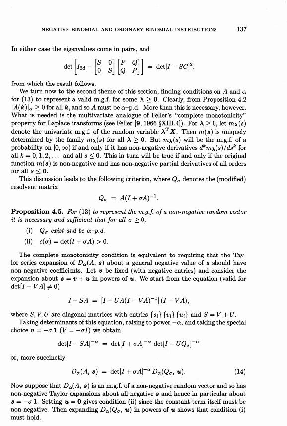
NEGATIVE BINOMIAL AND ORDINARY BINOMIAL DISTRIBUTIONS 137
In either case the eigenvalues come in pairs, and
det hd. ~S O' 0 S
P Q Q P
= det[7 — SC]2,
from which the result follows.We turn now to the second theme of this section, finding conditions on A and a
for (13) to represent a valid m.g.f. for some X > 0. Clearly, from Proposition 4.2 l-A(fc) |a > 0 for all k, and so A must be a-p.d. More than this is necessary, however. What is needed is the multivariate analogue of Feller’s “complete monotonicity” property for Laplace transforms (see Feller [9, 1966 §XIII.4]). For A > 0 , let m\ (s) denote the univariate m.g.f. of the random variable ATX . Then m(s) is uniquely determined by the family m\(s) for all A > 0. But m\(s) will be the m.g.f. of a probability on [0, oo) if and only if it has non-negative derivatives dkm\(s)/dsk for all k = 0 ,1 ,2 ,... and all s < 0. This in turn will be true if and only if the original function m(s) is non-negative and has non-negative partial derivatives of all orders for all s < 0.
This discussion leads to the following criterion, where Qa denotes the (modified) resolvent matrix
Qa = A{I + aA)~l .
Proposition 4.5. For (13) to represent the m.g.f. of a non-negative random vector it is necessary and sufficient that for all a > 0,
(i) Qa exist and be a-p.d.(ii) c (<t ) = det(I + a A) > 0.
The complete monotonicity condition is equivalent to requiring that the Taylor series expansion of Da(A, s ) about a general negative value of s should have non-negative coefficients. Let v be fixed (with negative entries) and consider the expansion about s = v + u in powers of u. We start from the equation (valid for d et[J -V M ]^ 0 )
I - S A = [I - UA(I - VA)~l] (I - VA),
where 5, V, U are diagonal matrices with entries {s*} {v*} {u^} and S = V + U.Taking determinants of this equation, raising to power —a, and taking the special
choice v — —a l (V = —aI) we obtain
det [ I-SA]~a = det[7 + aA]~a det[/ — UQcr]~a
or, more succinctly
Da(A, s) = det[/ + crA\~a Da(Qa, u). (14)
Now suppose that Da(A, s) is an m.g.f. of a non-negative random vector and so has non-negative Taylor expansions about all negative s and hence in particular about s = —a l . Setting u = 0 gives condition (ii) since the constant term itself must be non-negative. Then expanding Da(Q(T, u) in powers of u shows that condition (i) must hold.

138 D. VERE-JONES
Suppose conversely that (i) and (ii) hold for all cr > 0. Let v be a vector with negative entries and choose a > max |vi| so that a + Vi > 0. Also let s be a general vector. Then (14), together with assumptions (i) and (ii), implies that Da(A, s) has a power series expansion with non-negative coefficients in powers of Ui = Si + a = Si — Vi + Vi + cr. Since Vi + cr > 0 we may further expand each power of Ui in powers of Si — Vj, again with positive coefficients. Inserting the second expansion into the first gives a formal expansion, with non-negative coefficients, in powers of Si — Vi.
Provided the Vi are strictly negative, the series expansions are more than formal. In particular, the expansion of -Da(Q<T> s i ) has a non-zero radius of convergence and non-negative coefficients; hence its first singularity must appear for a positive value of s, and since the only singularities arise from zeros of the determinant det [I — sQa] they must be infinities. Equation (14) and condition (i) then lead to a contradiction unless the radius of convergence of this series at least equals cr. A similar argument starting from the expansion about a general negative v with | | < 0 shows that the series should converge at least for |s* — Vi\ < cr — max |v*|.
We conclude that if (i) and (ii) hold for all cr > 0, then Da(A,S) is completely monotone, and therefore represents an m.g.f.
The requirement for (13) to represent an m.g.f. places some constraints on the eigenvalues of A, although it does not seem possible to obtain a complete characterization in this way.
Note first that condition (ii) of Proposition 4.5 can be rephrased as(ii') all real, non-zero eigenvalues of A are positive.
Since the complex eigenvalues occur in conjugate pairs, whose products are positive, (ii') implies that the product of all non-zero eigenvalues is positive and hence that c(cr) > 0 for sufficiently large a. But then (ii') implies also that it has no zeros on the positive half-line and so c(cr) > 0 for all cr > 0. Conversely, if, for all cr > 0, c(a) > 0, the product of all non-zero eigenvalues must be positive and there can be no zeros of c(cr) on the positive axis, so no real eigenvalues can be negative.
More generally we have -
Proposition 4.6. For (13) to represent the m.g.f. of a non-negative random vector it is necessary that A, and all matrices obtained from A by multiplying the rows by arbitrary non-negative scalars, have eigenvalues with non-negative real parts only, and sufficient that they have real, non- negative eigenvalues only.
Consider again the m.g.f. of the random scalar ATX , with A > 0, which is of the form
m\(s) = det[/ — sAA}~a, A = diag(Ai,... , Ad).For this to represent the m.g.f. of a non-negative random variable it must be analytic for H(c(s) < 0, and so the eigenvalues of A A cannot have negative real parts.
Conversely, if KA has non-negative eigenvalues only, m\(s) can be factorized into a product of factors
( l - s 0 i ) - a,where 9{ is an eigenvalue of KA. This corresponds to a gamma distribution r(a , 1/di), and shows that m\(s) itself is the m.g.f. of a sum of such gamma variates.
NEGATIVE BINOMIAL AND ORDINARY BINOMIAL DISTRIBUTIONS 139
This being true for all A > 0, the multivariate form for m(s) must also be the m.g.f. of a non-negative random vector.
Conjugate pairs of eigenvalues a ± ib, with a > 0, contribute oscillatory terms to the density, and may or may not cause the density to become negative, the exact situation depending on the other eigenvalues as well as the values of a, b, and a.
As in the discussion to Proposition 4.5 it is easy to see that if the resolvent Qa is a-p.d., then it is also a-p.d. for any a' < a. The essential consideration is therefore the behaviour of Qa as a —» oo, which is related to properties of the inverse or adjugate matrix of A. If the inverse A~1 exists, then
aQc = ( i + = I - - A ~ 1 + \ a -'2 - . . . .\ a J a crz
In this case (crQ^u ~ 1 — /cr as a —> oo, while for i ^ j , (crQa)ij ~ —a^/cr.If A is singular, these rates of convergence may be altered, but as Griffiths
[13, 1984] pointed out, if we write
c(<7) = a det(^4 + cr-1/) > 0, (15)
then we can assert quite generally that
c(a)[crQG - /] —► -adj(A) (<r -* oo),
where c(a) is 0(cru+1), v being the order of 0 as a root of det(AI - A).This discussion suggests that it might be possible to frame simple conditions for
Qa to be a-p.d. for large a in terms of A~1 or adj (A). Looking at the cn-permanents in more detail, however, this hope is frustrated by the different rates of convergence in the a —permanents of different orders. If A is non-singular, for example, every given a-permanent will ultimately become non-negative, yet there may be no finite value of a for which they are all simultaneously non-negative.
The situation is much better in regard to infinite divisibility, corresponding to the requirement that Qa be u-p.d. That is because Griffiths’ cycle conditions (see Proposition 3.12) reduce to a finite set of conditions, all of which will be ultimately satisfied if they are satisfied in the limit.
Suppose then that ma(s ) is infinitely divisible, so that all Qa are w-p.d. From the condition
CQ„(i) > 0 i / 0, |i| > 1,we can immediately deduce that Cy{i) > 0 for V = —adj A. Note that the diagonal elements of —adj A are not in general non-negative, so it is not the case that V itself is w-p.d., at least in general.
For the converse, suppose first that A~x exists, so that as a —► oo
v{Qa)u ~ 1 - a^/a.
For sufficiently large cr, therefore, we should have {Qa)u > 0. Moreover the cycle conditions for Qa will follow from those for V at least if the latter hold with strict inequality. Finally, the condition c(a) > 0 for all cr > 0 is needed to ensure that Qa is u-p.d. for all a > 0. Thus, if A is non-singular, infinite divisibility of (13) follows from conditions (i) and (ii) of Proposition 4.7 below, if (i) holds with strict inequality.

140 D. VERE-JONES
If A is singular, then we may replace A by A + s I, and observe that if the cycle conditions hold for V with strict inequality, then they hold also for adj(A + si) , with s sufficiently small, so that the preceding arguments can be applied to Da(A + s i , s). Then letting s —► 0 the infinite divisibility of Da(A, s) follows from the continuity theorem for m.g.f.’s.
Proposition 4.7. In order that (13) represent the m.g.f. of an infinitely divisible distribution it is necessary that, if V = —adjA, c(cr) = det(/ + a A), and Cy(i) is defined as in (12),
(i) Cyii) > 0 - for all elementary cycles i ^ 0, |t| > 1;(ii) c (<t ) > 0 for all a > 0,
and sufficient that (i) and (ii) hold with strict inequality in (i).
We recall that condition (ii) is equivalent to the requirement that all real eigenvalues of A be non-negative.
If A is non-singular, and we set
Q* = I- (<rA)~\
Pa(Ql; z) = [det(/ — Q^)/det(/ — ZQ*)]a,
then, following Griffiths [13, 1984] we may observe that if (i) holds, even without strict inequality, and det A > 0, then Q*a is u-p.d. and so (see Section 5 below) Pa(Q*',z) is the p.g.f. of an infinitely divisible discrete distribution. Moreover, putting Zi = e~SitG and letting a —> oo, we find
Pa(Ql, z) - Da(A- s)
showing, from the continuity theorem again, that Da(A; s) is an infinitely divisible m.g.f.
Thus an alternative set of sufficient conditions in Proposition 4.7 is that (i) holds and that A be non-singular with det A > 0.
Example 4.8.
2 1 -1 3 h-* - 1 1'1 2 1 y = -adj A = - -1 1 1
-1 1 2 4 1 -1 1
Then det A = 0, and A is symmetric and positive semidefinite. Thus from Proposition 4.3, A is a-p.d. for a = On the other hand \A\a = a(a + l)(a — |) which is negative for 0 < a < so that A is not u-p.d. This follows also from the fact that the elementary cycle condition fails for A.
Examining crQa we find that as a —> oo, aQ a —► | A while det(7 -I- a A) = (l + f<x)2 >0 . Thus Proposition 4.5 suggests that Da(A; z) is an m.g.f. whenever A is a-p.d. Clearly the m.g.f. is not infinitely divisible, as follows also from the the fact that the cycle condition fails for V.

NEGATIVE BINOMIAL AND ORDINARY BINOMIAL DISTRIBUTIONS 141
It may be conjectured that A is a-p.d. for every a > \ , and also that Da(A\ z) will be an m.g.f. for every a > |, but we have not been able to establish this. Even for such a simple example, we do not have a complete picture of when the form(13) can be associated with a probability distribution.
5. Application to the Multivariate Negative Binomial Distribution
Here we consider a non-negative discrete random vector X with p.g.f. of the form
P(z) = Da(A, z - 1), (16)
where a > 0 and A is d x d.An alternative and equivalent form is obtained by setting Q = A(I + A)~l
(so that A = Q(I — Q)-1 ), and writing c(a) = det( / -I- A)~a = det(7 — Q)a. We have then
P(z) = c(a)Da(Q, z)= [d e t ( I -Q )/ d e t ( I -Z Q ) ]a. (17)
We follow the same pattern of development as in the previous section.
Proposition 5.1. Given that (16) represents the p.g.f. of the discrete random vector X , the marginal distribution of the subset (X ^ , X i2, . . . ,Xir), r < d, has a p.g.f. of the same form with the same value of a and with A replaced by the submatrix formed from A by deleting all rows and columns with indices not included zn the set . *tj- >
In particular, the distribution of the univariate marginals X{ are negative binominal with p.g.f.’s of the form
[ l - a i i ( 2 - l ) ] ~ a = [(1 -qi )/(l ~qiz)]a,
where = a « /( l + a«) (but $ ^ qu).
Proposition 5.2. Given that (16) represents the p.g.f. of the discrete random variable X, then
(i) the multivariate factorial moments can be represented as a-permanents of A and its derived matrices:
m[fcJ = E [J if1' , . . . = |-4(*)|„ (X M = X ( X - 1) . . . ( X - r + 1))
(ii) the corresponding factorial cumulants are given by the trace terms of A
C[k\ = atTA(k).
(iii) the multivariate probabilities can be represented as a-permanents of Q : if c(a) = det( / — Q)a, then
pk = Probpfr = h , i = 1 ,2 ,... ,d) = .I ll W

142 D. VERE-JONES
(iv) the corresponding Khinchin functions can be represented as the trace terms of Q :
X o = o l log c(a),X k = atiQ(k), ( *^0) .
The Khinchin functions are the coefficients in the expansion of \og P(z) about z = 0. In the case of a compound Poisson distribution the ratios X k / X o represent the probabilities in the compounding distribution. See Daley and Vere-Jones [7, 1988, Ch. 5] for a brief introduction and discussion of their relations to other properties.
Prom (i) and (ii) we readily obtain the special casesE(Xi) — Ol da 5
E (X iX j) 2 ,— Ol da djj “r Ol dij dji 9
Var X , — ol d^ "j- Qi da 5C a v (X „ X /) — ol d{j dji •
Any one of the families of coefficients ra^], C[*.], P[k\ and X[k] can be represented in terms of any of the others. Again there is a brief discussion of this circle of ideas in Ch. 5 of Daley and Vere-Jones [7, 1988]. In the present case the most interesting of these relations are those between the factorial moments and the probabilities, and vice versa, as these provide a generalisation to a-permanents of the well- known Fredholm expansions which occur in the theory of integral equations, and are expressed in terms of determinants. The link is the fact that the matrix Q solves the “integral equation”
Q = A - Q A .
Then the a-permanents of Q, which arise in the expansion of P(z) about z = 0, can be represented as a series in the a-permanents of A, which arise in the expansion of P (z ) about z = 1. The coefficients can be obtained by differentiating (16), or more obviously by expanding out the powers of (Zi — 1) in (16) and collecting terms. Reversing the process gives the a-permanents of A as a series of a-permanents derived from Q. The results can be expressed very simply for all a and take the following form.
Proposition 5.3.
0) - n(W )p(fc) = c(Q)l<3(*;)l« = E m rT rW fc+>)!«<i=i j> o
(ii) m[k] = |i4(fc)|a =j> o n
,i= 1 (JiV -Pk+j = c(a) 22
j> o n OiO\Q(k+j)\a.
If a = — 1 they correspond to the matrix equivalent of the expansion of the “Fredholm minor” in determinants, and if a = 1 they correspond to an analogous expansion in terms of permanents. The possibility of such permanent expansions has been noted by several authors, as mentioned in the introduction.
NEGATIVE BINOMIAL AND ORDINARY BINOMIAL DISTRIBUTIONS 143
There is a direct link between the multivariate negative binomial distributions considered here and the multivariate gamma distributions of the previous section.
Proposition 5.4. If Da(A, z ) represents the m.g.f. of a non-negative random vector X , then Da(A, z — 1) represents the p.g.f. of a discrete non-negative random vector 7 , and the moments and cumulants of X are equal to the corresponding factorial moments and cumulants of 7 .
This is just a special case of the well-known formulae for the representation of a mixed Poisson distribution, with the gamma distribution of Section 4 acting as the mixing distribution.
The converse is not true without supplementary conditions, as can be seen from comparing Proposition 4.5 with its analogue for the negative binomial distribution stated below.
Proposition 5.5. Necessary and sufficient conditions for (16) to represent the multivariate p.g.f. of a discrete, non-negative random variable are
(i) Q = A(I + A)-1 exists and is a-p.d.(ii) det(7 -I- A)~x = det (I — Q) > 0.
Condition (i) ensures that Da(Q, z) has an expansion with non-negative terms; condition (ii) ensures that the same is true for P(z). It is clear that when both conditions are satisfied, P{ 1) = 1.
The distinction between (i) and (ii) above and the corresponding conditions in Proposition 4.5 is that the conditions here are required only for cr = 1. To see that the distinction is not vacuous, consider the 2x2 case, which can be completely analysed (compare Griffiths [13, 1984] and Griffiths and Milne [14, 1987]) as follows.
Proposition 5.6. Let d — 2 in (13) and (16). Then
(i) A is a-p.d. if and only if an > 0, 022 > 0 and ai2 a2i > 0;(ii) (16) is p.g.f if and only if (i) holds, and in addition an a22 — ^12 «2i >
Parts (ii) and (iii) follow from computing Q and Qa, applying Propositions 5.5 and 4.5 respectively, and substituting the necessary and sufficient conditions from(i) for these matrices to be a-p.d.
(—o-u, —a 22);(iii) (13) is a p.g.f. if and only if (i) holds, and in addition an 022—^12 ^21 >
0.
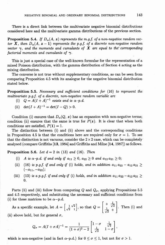
As a specific example, let A = i ^ , so that Q = 1 • Then (i) andL v 2 1 J —— 0
01
which is non-negative (and in fact a-p.d.) for 0 < a < 1, but not for cr > 1.

144 D. VERE-JONES
The conditions for infinite divisibility of (16) follow immediately from the general results of Section 3. It is enough to replace the condition that Q is a-p.d. in Proposition 5.5(i) by the condition that it is u-p.d. Invoking Griffiths’ elementary cycle criterion we obtain the following statement.
Proposition 5.7. In order that (16) represent the p.g.f. of an infinitely divisible discrete distribution it is necessary and sufficient that
(i) Qa ^ ® — 1,2,... , d,(ii) the elementary cycle conditions of Proposition 3.12 hold with B = Q,(iii) det(7 + A)-1 = det (I — Q) > 0.
The result represents a minor extension of that in Griffiths and Milne [14, 1987], who either consider the case that A is non-negative definite, when condition (iii) is automatically satisfied, or require that Q be non-negative definite with maximum eigenvalue strictly less than unity.
6. Application to the Multivariate Binomial Distribution
In this section we consider multivariate discrete distributions with p.g.f.’s of the form
P(z) = D - m(-A , z - 1) = det[J + [Z - I)A]m (18)
or equivalently, writing Q = A( 1 — A)-1 , and setting c(m) = det(7 — A)m = det (7 + Q )-m,
P{z) = c(m) D - m( - Q , z) = [det(J + ZQ)/det(7 4- Q)]m. (19)
For the latter form to be defined we must assume that 7 - A is non-singular, an assumption which will be made throughout this section. An expansion with non-negative coefficients is possible only if m is an integer. When (18) and (19) represent a valid p.g.f., the analogues of Propositions 5.1, 5.2, and 5.3 for the marginal distributions, factorial moments and cumulants, probabilities, Khinchin functions hold word for word with the substitutions of —m for a , —A for A, and —Q for Q. We forebear from rewriting the results in detail. However, it may be worth noting that the 1-dimensional marginals are all of binomial form with p.g.f.’s.
[1 + au(z — l)]m = [ ( l+ q i z)/(l + qi)}rn,
where qi = an/(l — an), and that first and second moments are given by
E(Xi) — man(^Cj Cj) — m da djj m dij dj%
Var Xi = man ~ m dnCov(Jfj X*j) — m dij (ij .
The negative sign in the covariance shows that, in contrast to the previous case, the component variables are negatively correlated ( “antibunching” ).

NEGATIVE BINOMIAL AND ORDINARY BINOMIAL DISTRIBUTIONS 145
A simple example occurs when A is the matrix of rank 1 in which all elements in the z-th row are equal to pi, i = 1,... , d, with Y^Pi = 1- Then only the first order terms in the characteristic polynomial are non-zero, so that
d “p (z) = 1 + £ ( * - ! ) *
lwhich is the p.g.f. of the multinomial distribution on d terms.
Conditions for (18) to represent a valid p.g.f. are much simpler than in the previous cases.Proposition 6.1. The function (18) represents a valid p.g.f. either for all integers m or for none. The necessary and sufficient condition for the former case to hold is that, for all k < d, the symmetrically placed minors from Q be non-negative (i.e., that Q be (—1 )-p.d.).
This is obviously sufficient, directly from the expansion of the characteristic polynomial of Q.
Suppose that (18) represents a p.g.f. for some m > 1. Then as z —* 0, P(z) —* det[7 + Q]~m > 0 (the inequality being strict since we assume I — A to be non-singular). Hence also the coefficients in [det(7 -t- QZ)]m must be nonnegative. We need to show that if this is true for some m > 1, then det [I + QZ] itself has an expansion with non-negative coefficients.
We shall establish this by induction on the order d of the matrix. If d = 1 it is equivalent to the requirement that, if (1 +az)m has non-negative coefficients, then a > 0; this is clearly true, for all m. Write for brevity
D(z) = det[7 -1- ZQ\ = 1 + qj Zj + qij Zj Zj + .. . + qi,2,... ,dZi .. . zd
and suppose that det [I + ZQ]m has non-negative coefficients.By the induction hypothesis (restricting Q to a submatrix) we may suppose
qi > 0, qij > 0, . . . up to and including all terms of order d — 1 .Now consider the coefficient of (z\ .. . Zd-i)mZd in the expansion of D(z)m, which
by assumption is non-negative. The only term contributing to this coefficient is(qi,2,... ,d—i )m—1 qi,2,... ,di With qi,2,...,d-i > 0.
It follows that <71,2,... td > 0 whenever ,d-i is positive. Even if the latter is zero, the same conclusion would follow if any of the ( dd1) terms of order d — 1 in D (z ) were non-zero. If all terms of order d — 1 are zero, we consider instead the coefficient of (z\ . .. zd- 2)m Zd-i Zd, and observe that the only term contributing to this, which does not contain a zero term of order (d — 1 ), is
(91,2,... ,d—2)m_1 Qi,2,... ,d, with 91,2,... ,d-2 > 0.Hence we reach a similar conclusion unless all terms of order d — 2 are zero. We may continue this argument until finally we reach the zero order term which is always positive. This completes the induction and so establishes the necessity of the conditions.
If the matrices A and Q are symmetric, then the condition in Proposition 6.1 is nothing other than the usual requirement that Q be positive semidefinite in the classical sense. In this case we can form an equivalent condition on A, namely that A be positive semidefinite with maximum eigenvalue strictly less than unity.
146 D. VERE-JONES
7. Mixtures and Stochastic Processes
In this section we note briefly two extensions of the previous results.The first concerns the more general classes of distributions defined by taking mix
tures with respect to the parameter a. Consider, for example, the negative binomial distributions discussed in Section 5. Then the p.g.f. for the mixture distribution can be written as
II(z) = f?a{exp[—a:log det(J — ZA )]} = x[l°g det(J — ZA)],
where x(s) = E[e~sa] is the Laplace transform of the distribution for a.The factorial moments in this case will be given by expressions analogous to the
a-permanents but with the powers of a replaced by the corresponding moments fim = E[am]. Thus for example the expression (i) of Proposition 5.2 becomes
mw = E [x [h) ... X , = Ea {|A(*)U}
where for any matrix B of order k
{II a } P'm(a) lii & 2 ,C7
nmw = £ [am<-)]and as before m(c) denotes the number of cycles making up the permutation a and the summation is taken over all possible permutations of the indices.
Similarly the cumulants will be defined by
ck = E(a)trA(k).
The probabilities will be defined by similar expressions with the power of a in the a-permanents of Q(k) in Proposition 5.2(iii) replaced by coefficients
vm = E[c{a) am] = £[det(/ - Q)a am].
Analogous results can be written down for the other classes of distributions, but we omit the details.
The second type of extension is to stochastic processes, and is suggested by the “nesting” property of the marginal distributions in each of the three multivariate families considered. For each case, and fixed a, define a consistent family of finite dimensional marginal distributions by selecting submatrices from an appropriately defined infinite dimensional matrix and use these submatrices to define the marginal m.g.f.’s or p.g.f.’s as the case may be.
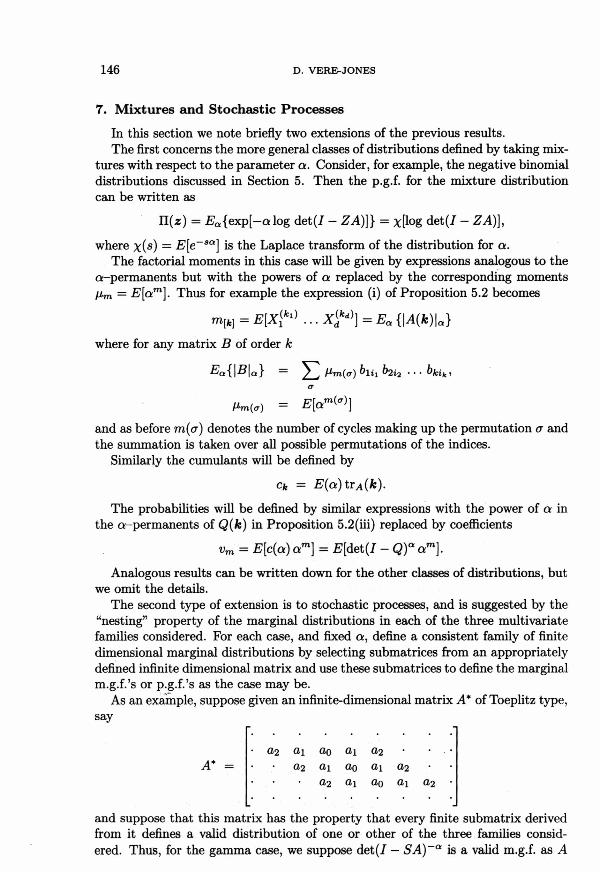
As an example, suppose given an infinite-dimensional matrix A* of Toeplitz type, say
A* =a,2 a i do ai a2 •
(Z2 CL\ <2o Oj2<22 d\ a o fli &2
and suppose that this matrix has the property that every finite submatrix derived from it defines a valid distribution of one or other of the three families considered. Thus, for the gamma case, we suppose det(/ — SA)~a is a valid m.g.f. as A

NEGATIVE BINOMIAL AND ORDINARY BINOMIAL DISTRIBUTIONS 147
successively runs through the submatrices
A = [ao], A = do di do di dj, A = di do di
CiOm aj di do_etc.
Then given any finite set of indices ii , . . . , id we can define the distribution corresponding to the set of random variables X ^ , Xid, by supposing it to be of the given type with matrix A extracted from A* by considering only the rows and columns with indices i\,. .. , id- The nesting property implies that all consistency conditions will be satisfied, and so a well-defined, stationary stochastic process will result, in which the marginal distributions are either gamma, negative binomial, or binomial.
In the gamma case, the matrix A* has the interpretation that the squares of its elements are proportional to the autocovariances:
CovpQ, X i+k) = aa\ k = 0 ,1 ,2 , . . . .The same interpretation holds for the off-diagonal elements in the negative bi
nomial case, but on the diagonal we haveVarXi = aog + aao.
In the binomial case these interpretations are replaced by CovpQ, Xi+k) = —ma\
Var Xi = mao — ma^.
Acknowledgements. The theme of this paper has been a continuing interest over a number of years, and I would like to express my thanks to numerous correspondents who have been kind enough to send reprints and references which have helped to fill some of the historical gaps or point to new links and possible applications. I am also grateful to an anonymous referee for a meticulous reading of the manuscript which has spared me from many embarassing slips.
References
1. G. Andrews, Collected Papers of P. A. MacMahon, Volume 1 of Combinatorics, M.I.T. Press, Cambridge, (Mass.), 1979.
2. C. Benard and O. Macchi, Detection and emission processes of quantum particles in a chaotic state, J Math. Phys. 14 (1973), 155-167.
3. A. Blokhuis and J. Seidel, An introduction to multilinear algebra and some applications, Philips J. Res. 39 (1984), 111-120.
4. D. Brillinger, Time Series : Data Analysis and Theory, Holt, Rinehart and Winston, New York, 1975.
5. A. Cayley, Sur les determinants gauches, Crelle’s Journal, xxxviii (1847), 94-96.
6. W. Chu, Some algebraic Identities Concerning Determinants and Permanents, Preprint, 1988.
7. D. Daley and D. Vere-Jones, An Introduction to the Theory of Point Processes, Springer, New York and C., 1988.
8. N. de Bruijn, The Lagrange-Good inversion formula and its applications to integral equations, J. Math. Anal, and Appn. 92 (1983), 397-409.

148 D. VERE-JONES
9. W. Feller, Introduction to Probability Theory and its Applications, Volume II, Wiley, New York, 1966.
10. W. Feller, Introduction to Probability Theory and its Applications, Volume I, Wiley, New York, Third Edition, 1968.
11. D. Goodman and M. Dubman, Theory of time-varying spectral analysis and complex Wishart matrices, in Multivariate Analysis II (P. Krishnaiah, ed.), Academic Press, New York, 1969.
12. I. Goulden and D. Jackson, Combinatorial Enumeration, 1983.13. R. Griffiths, Characterization of infinitely divisible multivariate gamma distri
butions, J. Multivariate Anal. 15 (1984), 13-20.14. R. Griffiths and R. Milne, A class of infinitely divisible multivariate negative
binomial distributions, J. Multivariate Anal. 22 (1987), 13-23.15. D. Kershaw, Permanents in Fredholm’s theory of integral equations, J. Integral
Equations 1 (1979), 281-290.16. P. Levy, The arithmetic character of the Wishart distribution, Proc. Camb.
Phil. Soc. (Math. Phys. Sci.) 44 (1948), 295-297.17. D. Littlewood, The Theory of Group Characters, Oxford University Press,
Second Edition, 1950.18. E.K. Lloyd, Some little-known results of MacMahon on permanents,
Ars Combinatorica 16A (1983), 319-323.19. E. Lukacs and R. Laha, Applications of Characteristic Functions, Griffin,
London, 1964.20. O. Macchi, The coincidence approach to stochastic point processes, Adv. Appl.
Prob. 7 (1975), 83-122.21. P. MacMahon, Combinatory Analysis, Volume 1, Cambridge University Press,
Cambridge, 1915.22. H. Mine, Permanents, Addison-Wesley, Reading, 1978.23. T. Muir, Contributions to the history of determinants 1900-1920, Blackie, Lon
don, 1930.24. K. Parthasarathy and K. Schmidt, Positive Definite Kernels, Continuous Ten
sor Products, and Central Limit Theorems of Probability Theory, in Lecture Notes in Mathemetics (Number 272), Springer, New York etc., 1972.
25. I. Schur, Uber endliche gruppen und hermetische forrnen, Math. Zeit. 1 (1918), 184-207.
26. J. Schwinger, The theory of quantized fields V, Phys. Rev. 93 (1954), 615-628.27. D. Vere-Jones, An identity involving permanents, Linear Algebra and its
Applications 63 (1984), 267-270.28. D. Vere-Jones, Alpha Permanents and their Applications, Preprint, (VUW),
1987.29. D. Vere-Jones, A generalization of permanents and determinants, Linear
Algebra and its Appns. I l l (1988), 119-124.

NEGATIVE BINOMIAL AND ORDINARY BINOMIAL DISTRIBUTIONS 149
30. P. Whittle, Probability, Penguin, 1970.31. H. Wilf, A mechanical counting method and combinatorial applications,
J. Combinatorial Theory 4 (1968), 246-258.
D. Vere-JonesInstitute of Statistics and Operations ResearchVictoria University of WellingtonPO Box 600WellingtonNEW ZEALANDd vj @isor. vuw. ac. nz
