almansi formula on the sphere and new cubature … paradigm - areas multivariate splines also on...
TRANSCRIPT

Almansi Formula on the Sphere and New CubatureFormulas with Error Bounds
Polyharmonic Paradigm
Ognyan Kounchev
Institute of Mathematics and Informatics, Bulgarian Academy of Sciences, visiting MaxPlanck Institute of Mathematics, Leipzig
Signals, Images, and Approximation, Bernried, March 2016
Ognyan Kounchev (Institute of Mathematics and Informatics, Bulgarian Academy of Sciences, visiting Max Planck Institute of Mathematics, Leipzig)Almansi Formula on the Sphere and New Cubature Formulas with Error BoundsSignals, Images, and Approximation, Bernried, March 2016 1
/ 23

The speaker‘s attendance at this conference was sponsored by
the Alexander von Humboldt Foundation.
http://www.humboldt-foundation.de
Ognyan Kounchev (Institute of Mathematics and Informatics, Bulgarian Academy of Sciences, visiting Max Planck Institute of Mathematics, Leipzig)Almansi Formula on the Sphere and New Cubature Formulas with Error BoundsSignals, Images, and Approximation, Bernried, March 2016 2
/ 23

Main purpose of the talk
”Beauty is the first test: there is no permanent place in the world forugly mathematics.”
”It is one of the first duties of a professor, for example, in anysubject, to exaggerate a little both the importance of his subject andhis own importance in it.”
”Mathematical fame, if you have the cash to pay for it, is one of thesoundest and steadiest of investments.”
G. G. Hardy, A Mathematician’s Apology
Ognyan Kounchev (Institute of Mathematics and Informatics, Bulgarian Academy of Sciences, visiting Max Planck Institute of Mathematics, Leipzig)Almansi Formula on the Sphere and New Cubature Formulas with Error BoundsSignals, Images, and Approximation, Bernried, March 2016 3
/ 23

Polyharmonic Paradigm - what is it ?
Main idea is: Use solutions of the polyharmonic equation in Rn :
∆Nu (x) = 0 in domain D
instead of multivariate polynomials P (x) .
Generalize the 1D odd-degree polynomials P2N−1 (t) by Hermiteinterpolation: they solve the Boundary Value problem
d2N
dt2NP2N−1 (t) = 0
d j
dt jP2N−1 (0) = cj for j = 0, 1, ..., N − 1
d j
dt jP2N−1 (1) = dj for j = 0, 1, ..., N − 1
In multivariate case - solution of Boundary Value problem:
∆Nu (x) = 0 in domain D
∆ju (x) = gj (x) for x ∈ ∂D
Ognyan Kounchev (Institute of Mathematics and Informatics, Bulgarian Academy of Sciences, visiting Max Planck Institute of Mathematics, Leipzig)Almansi Formula on the Sphere and New Cubature Formulas with Error BoundsSignals, Images, and Approximation, Bernried, March 2016 4
/ 23

Polyharmonic Paradigm - what is it ?
Main idea is: Use solutions of the polyharmonic equation in Rn :
∆Nu (x) = 0 in domain D
instead of multivariate polynomials P (x) .Generalize the 1D odd-degree polynomials P2N−1 (t) by Hermiteinterpolation: they solve the Boundary Value problem
d2N
dt2NP2N−1 (t) = 0
d j
dt jP2N−1 (0) = cj for j = 0, 1, ..., N − 1
d j
dt jP2N−1 (1) = dj for j = 0, 1, ..., N − 1
In multivariate case - solution of Boundary Value problem:
∆Nu (x) = 0 in domain D
∆ju (x) = gj (x) for x ∈ ∂D
Ognyan Kounchev (Institute of Mathematics and Informatics, Bulgarian Academy of Sciences, visiting Max Planck Institute of Mathematics, Leipzig)Almansi Formula on the Sphere and New Cubature Formulas with Error BoundsSignals, Images, and Approximation, Bernried, March 2016 4
/ 23

Polyharmonic Paradigm - areas
Multivariate Splines also on manifolds: Consult the bookMultivariate Polysplines. Applications to Numerical and WaveletAnalysis, Academic Press, 2001.
Multivariate Wavelets, also on some manifolds: Chui typepolyharmonic wavelets in 2001 ; Daubechies type subdivisionwavelets - with N. Dyn, D. Levin, H. Render – in progress since 2010.
Multivariate (Polyharmonic) Subdivision, also on manifolds: N.Dyn, D. Levin, H. Render
A new point of view on many other areas: Several Complex Variables,Riemann surfaces and Algebraic Geometry, etc.
Several mathematical lives will be necessary
Multivariate Moment problem, Operator theory (as Tensorrepresentations), and multivariate Quadrature (= Cubature) - thepresent talk
Ognyan Kounchev (Institute of Mathematics and Informatics, Bulgarian Academy of Sciences, visiting Max Planck Institute of Mathematics, Leipzig)Almansi Formula on the Sphere and New Cubature Formulas with Error BoundsSignals, Images, and Approximation, Bernried, March 2016 5
/ 23

One-dimensional reminder on quadrature formulas
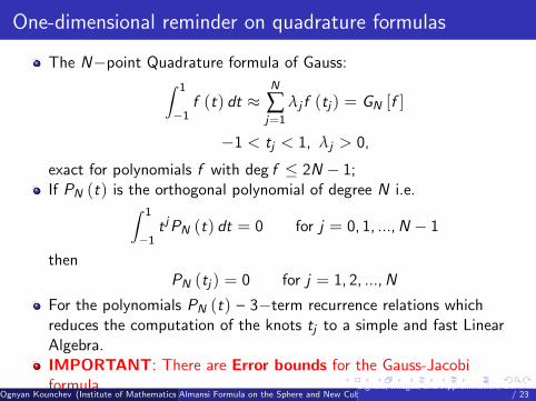
The N−point Quadrature formula of Gauss:∫ 1
−1f (t) dt ≈
N
∑j=1
λj f (tj ) = GN [f ]
−1 < tj < 1, λj > 0,
exact for polynomials f with deg f ≤ 2N − 1;
If PN (t) is the orthogonal polynomial of degree N i.e.∫ 1
−1t jPN (t) dt = 0 for j = 0, 1, ..., N − 1
thenPN (tj ) = 0 for j = 1, 2, ..., N
For the polynomials PN (t) – 3−term recurrence relations whichreduces the computation of the knots tj to a simple and fast LinearAlgebra.IMPORTANT: There are Error bounds for the Gauss-Jacobiformula.
Ognyan Kounchev (Institute of Mathematics and Informatics, Bulgarian Academy of Sciences, visiting Max Planck Institute of Mathematics, Leipzig)Almansi Formula on the Sphere and New Cubature Formulas with Error BoundsSignals, Images, and Approximation, Bernried, March 2016 6
/ 23

One-dimensional reminder on quadrature formulas
The N−point Quadrature formula of Gauss:∫ 1
−1f (t) dt ≈
N
∑j=1
λj f (tj ) = GN [f ]
−1 < tj < 1, λj > 0,
exact for polynomials f with deg f ≤ 2N − 1;If PN (t) is the orthogonal polynomial of degree N i.e.∫ 1
−1t jPN (t) dt = 0 for j = 0, 1, ..., N − 1
thenPN (tj ) = 0 for j = 1, 2, ..., N
For the polynomials PN (t) – 3−term recurrence relations whichreduces the computation of the knots tj to a simple and fast LinearAlgebra.
IMPORTANT: There are Error bounds for the Gauss-Jacobiformula.
Ognyan Kounchev (Institute of Mathematics and Informatics, Bulgarian Academy of Sciences, visiting Max Planck Institute of Mathematics, Leipzig)Almansi Formula on the Sphere and New Cubature Formulas with Error BoundsSignals, Images, and Approximation, Bernried, March 2016 6
/ 23
One-dimensional reminder on quadrature formulas
The N−point Quadrature formula of Gauss:∫ 1
−1f (t) dt ≈
N
∑j=1
λj f (tj ) = GN [f ]
−1 < tj < 1, λj > 0,
exact for polynomials f with deg f ≤ 2N − 1;If PN (t) is the orthogonal polynomial of degree N i.e.∫ 1
−1t jPN (t) dt = 0 for j = 0, 1, ..., N − 1
thenPN (tj ) = 0 for j = 1, 2, ..., N
For the polynomials PN (t) – 3−term recurrence relations whichreduces the computation of the knots tj to a simple and fast LinearAlgebra.IMPORTANT: There are Error bounds for the Gauss-Jacobiformula.
Ognyan Kounchev (Institute of Mathematics and Informatics, Bulgarian Academy of Sciences, visiting Max Planck Institute of Mathematics, Leipzig)Almansi Formula on the Sphere and New Cubature Formulas with Error BoundsSignals, Images, and Approximation, Bernried, March 2016 6
/ 23

Jacobi’s point of view
For a weight function w (t) > 0 (originally,
w (t) = (1 + t)α (1− t)β) let
f (t) = g (t)w (t) .
We have N−point Gauss-Jacobi formula∫ 1
−1f (t) dt ≈
N
∑j=1
λjg (tj ) =: GJN [f ]
where PN (tj ) = 0 and λj > 0, but∫ 1
−1t jPN (t)w (t) dt = 0 for j = 0, 1, ..., N − 1.
Example: Compute ∫ 1
0g (t)
1√t
dt
for a polynomial g (t) in two ways: using Gauss GN , or usingGauss-Jacobi GJN for w (t) = 1√
t.
Ognyan Kounchev (Institute of Mathematics and Informatics, Bulgarian Academy of Sciences, visiting Max Planck Institute of Mathematics, Leipzig)Almansi Formula on the Sphere and New Cubature Formulas with Error BoundsSignals, Images, and Approximation, Bernried, March 2016 7
/ 23

Multidimensional case - challenges
A big discrepancy between the 1D case and the multi-dimensionalcase
There is no Jacobi’s point of view!
Cubature formulas –Orthogonal polynomials of several variables byHermite 1889, Appelle, Radon, Sobolev, etc.
Solve equations for finding λj and xj – problems with error bounds.
Ognyan Kounchev (Institute of Mathematics and Informatics, Bulgarian Academy of Sciences, visiting Max Planck Institute of Mathematics, Leipzig)Almansi Formula on the Sphere and New Cubature Formulas with Error BoundsSignals, Images, and Approximation, Bernried, March 2016 8
/ 23

Cubature formulas
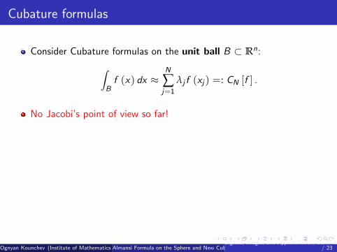
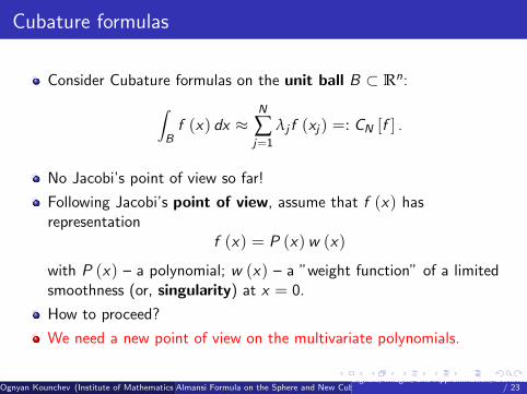
Consider Cubature formulas on the unit ball B ⊂ Rn:∫B
f (x) dx ≈N
∑j=1
λj f (xj ) =: CN [f ] .
No Jacobi’s point of view so far!
Following Jacobi’s point of view, assume that f (x) hasrepresentation
f (x) = P (x)w (x)
with P (x) – a polynomial; w (x) – a ”weight function” of a limitedsmoothness (or, singularity) at x = 0.
How to proceed?
We need a new point of view on the multivariate polynomials.
Ognyan Kounchev (Institute of Mathematics and Informatics, Bulgarian Academy of Sciences, visiting Max Planck Institute of Mathematics, Leipzig)Almansi Formula on the Sphere and New Cubature Formulas with Error BoundsSignals, Images, and Approximation, Bernried, March 2016 9
/ 23
Cubature formulas
Consider Cubature formulas on the unit ball B ⊂ Rn:∫B
f (x) dx ≈N
∑j=1
λj f (xj ) =: CN [f ] .
No Jacobi’s point of view so far!
Following Jacobi’s point of view, assume that f (x) hasrepresentation
f (x) = P (x)w (x)
with P (x) – a polynomial; w (x) – a ”weight function” of a limitedsmoothness (or, singularity) at x = 0.
How to proceed?
We need a new point of view on the multivariate polynomials.
Ognyan Kounchev (Institute of Mathematics and Informatics, Bulgarian Academy of Sciences, visiting Max Planck Institute of Mathematics, Leipzig)Almansi Formula on the Sphere and New Cubature Formulas with Error BoundsSignals, Images, and Approximation, Bernried, March 2016 9
/ 23

Our approach in the 2D case – in the disc B
We consider the Fourier expansions for general functions P and w ,where z = x + iy :
P (z) =∞
∑k=−∞
pk (r) e ikϕ z = re iϕ, r = |z |
w (z) =∞
∑k=−∞
wk (r) e ikϕ
and
pk (r) :=1
2π
∫ 2π
0P(re iϕ
)e−ikϕd ϕ; wk (r) :=
1
2π
∫ 2π
0w(re iϕ
)e−ikϕd ϕ
Hence,∫B f (z) dz is reduced to
I :=∫B
P (z)w (z) dz = 2π∞
∑k=−∞
∫ 1
0pk (r)w−k (r) rdr
Ognyan Kounchev (Institute of Mathematics and Informatics, Bulgarian Academy of Sciences, visiting Max Planck Institute of Mathematics, Leipzig)Almansi Formula on the Sphere and New Cubature Formulas with Error BoundsSignals, Images, and Approximation, Bernried, March 2016 10
/ 23

A remarkable representation of multivariate polynomials,2D case
Let P (x , y) be a polynomial in R2 satisfying ∆NP (x , y) = 0. Thenthe following remarkable Almansi representation holds
P (x , y) =∞
∑k=−∞
p̃k
(r2)
rke ikϕ z = r × e iϕ, r = |z |
where p̃k is a 1D polynomial of degree ≤ N − 1.
Hence, the polyharmonic degree N (in ∆N) is a generalization forthe one-dimensional degree N of the polynomials.
This is a fundamental point of the so-called PolyharmonicParadigm.
Ognyan Kounchev (Institute of Mathematics and Informatics, Bulgarian Academy of Sciences, visiting Max Planck Institute of Mathematics, Leipzig)Almansi Formula on the Sphere and New Cubature Formulas with Error BoundsSignals, Images, and Approximation, Bernried, March 2016 11
/ 23

The integral as infinite sum of 1-dim integrals
Hence, for polynomials P (x) we obtain for ρ = r2
I = ∑k
∫ 1
0pk
(r2)
rkwk (r) rdr = ∑k
∫ 1
0pk (ρ) w̃k (ρ) dρ;
Here the new weigth w̃k,` (ρ) is defined by
w̃k (ρ) dρ := rkwk (r) rdr =1
2ρ
k2 wk (
√ρ) dρ
Now we make a crucial assumption:
w̃k (ρ) ≥ 0 for all indices k .
For every k ∈ Z and N ≥ 1, we apply N−point Gauss-Jacobiquadrature: ∫ 1
0pk (ρ) w̃k (ρ) dρ ≈
N
∑j=1
pk (tj ;k) λj ;k
which is exact for polynomials pk satisfying deg pk ≤ 2N − 1.
Ognyan Kounchev (Institute of Mathematics and Informatics, Bulgarian Academy of Sciences, visiting Max Planck Institute of Mathematics, Leipzig)Almansi Formula on the Sphere and New Cubature Formulas with Error BoundsSignals, Images, and Approximation, Bernried, March 2016 12
/ 23

The cubature formula defined:
Now, let g (x) be a continuous function with Fourier expansion
g (x) = ∑k
gk (r) e ikϕ
The integral becomes∫B
g (z)w (z) dz = ∑k
∫ 1
0gk (r)wk (r) rdr
=1
2 ∑k
∫ 1
0gk (√
ρ) ρ−k2 ρ
k2 wk (
√ρ) dρ
≈ 1
2 ∑k
N
∑j=1
gk(√
tj ;k)
t− k
2j ;k × λj ;k
=: C (g)
Ognyan Kounchev (Institute of Mathematics and Informatics, Bulgarian Academy of Sciences, visiting Max Planck Institute of Mathematics, Leipzig)Almansi Formula on the Sphere and New Cubature Formulas with Error BoundsSignals, Images, and Approximation, Bernried, March 2016 13
/ 23

The miracle - Chebyshev inequality applied
Important to see convergence of C (g) , i.e.:
2C (g) = ∑k
N
∑j=1
gk(√
tj ;k)· t−
k2
j ;k · λj ;k < ∞.
The proof: application of the famous Chebyshev inequality.
We obtain∣∣∣∣∣ N
∑j=1
gk (tj ;k) · t− k
2j ;k · λj ;k
∣∣∣∣∣ ≤ C ‖g‖sup∫
wk (√
ρ) dρ
Further, we impose the condition
‖w‖ := ∑k,`
∫wk (√
ρ) dρ < ∞
Ognyan Kounchev (Institute of Mathematics and Informatics, Bulgarian Academy of Sciences, visiting Max Planck Institute of Mathematics, Leipzig)Almansi Formula on the Sphere and New Cubature Formulas with Error BoundsSignals, Images, and Approximation, Bernried, March 2016 14
/ 23

Final approximation of the Fourier coefficients
To finish the Cubature formula, approximate the coefficients gk (r) .In R2 we have have
gk (r) =1
2π
∫ 2π
0g(re iϕ
)e ikϕd ϕ
Hence, for integers M ≥ 1, the approximation is just the trapezoidal rule:
f(M)k (r) :=
2π
M
M
∑s=1
f(
re i2πsM
)e i
2πsM
For real-valued functions g , the final Cubature formula is:
∫B
g (z)w (z) dz ≈ π
M
K
∑k=0
N
∑j=1
M
∑s=1
λj ,k · t− k
2j ,k · e
i 2πsM · g
(√tj ,ke i
2πsM
)
Ognyan Kounchev (Institute of Mathematics and Informatics, Bulgarian Academy of Sciences, visiting Max Planck Institute of Mathematics, Leipzig)Almansi Formula on the Sphere and New Cubature Formulas with Error BoundsSignals, Images, and Approximation, Bernried, March 2016 15
/ 23
Exactness space
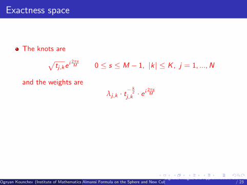
The knots are√tj ,ke i
2πsM 0 ≤ s ≤ M − 1, |k | ≤ K , j = 1, ..., N
and the weights are
λj ,k · t− k
2j ,k · e
i 2πsM
The formula is exact for the polynomials
P (x , y) = r2srke ikϕ = |z |2s zk
for 0 ≤ s ≤ 2N − 1; 0 ≤ k ≤ M − 1−K
Ognyan Kounchev (Institute of Mathematics and Informatics, Bulgarian Academy of Sciences, visiting Max Planck Institute of Mathematics, Leipzig)Almansi Formula on the Sphere and New Cubature Formulas with Error BoundsSignals, Images, and Approximation, Bernried, March 2016 16
/ 23

Exactness space
The knots are√tj ,ke i
2πsM 0 ≤ s ≤ M − 1, |k | ≤ K , j = 1, ..., N
and the weights are
λj ,k · t− k
2j ,k · e
i 2πsM
The formula is exact for the polynomials
P (x , y) = r2srke ikϕ = |z |2s zk
for 0 ≤ s ≤ 2N − 1; 0 ≤ k ≤ M − 1−K
Ognyan Kounchev (Institute of Mathematics and Informatics, Bulgarian Academy of Sciences, visiting Max Planck Institute of Mathematics, Leipzig)Almansi Formula on the Sphere and New Cubature Formulas with Error BoundsSignals, Images, and Approximation, Bernried, March 2016 16
/ 23

Nice properties of the Cubature formula – stability estimate
The coefficients satisfy the stability estimate∣∣∣∣∣ π
M
K
∑k=0
N
∑j=1
M
∑s=1
λj ,k · t− k
2j ,k · e
i 2πsM
∣∣∣∣∣ ≤ C1 ‖w‖ .
By a theorem of Polya and others, we have a stable Cubature formula.
Ognyan Kounchev (Institute of Mathematics and Informatics, Bulgarian Academy of Sciences, visiting Max Planck Institute of Mathematics, Leipzig)Almansi Formula on the Sphere and New Cubature Formulas with Error BoundsSignals, Images, and Approximation, Bernried, March 2016 17
/ 23

Error estimates
Due to the above, we have all nice Error estimates for theseCubature formula, w.r.t. all parameters K , N, M.
Details are available in arxiv: http://arxiv.org/abs/1509.00283
Ognyan Kounchev (Institute of Mathematics and Informatics, Bulgarian Academy of Sciences, visiting Max Planck Institute of Mathematics, Leipzig)Almansi Formula on the Sphere and New Cubature Formulas with Error BoundsSignals, Images, and Approximation, Bernried, March 2016 18
/ 23

Almansi formula for the spherical harmonics on the sphere
On the unit sphere S2 ⊂ R3 we consider the integral
Iw (f ) =∫
S2f (Θ)w (Θ) dσΘ with dσΘ = sin ϑd ϕdϑ
For Θ ∈ S2 we have the representation, with 0 ≤ ϕ < 2π and0 ≤ ϑ < π,
Θ1 = sin ϑ cos ϕ, Θ2 = sin ϑ sin ϕ, Θ3 = cos ϑ
We put x = cos ϑ, ϑ = arccos x . Then, for k = 0, 1, ...; |λ| ≤ k ,the spherical harmonics
{Y λk (Θ)
}on S2 are normalized as:
Y λk (Θ) = Nk,λ × e iλϕPλ
k (cos ϑ) = Nk,λ × e iλϕ(1− x2
) |λ|2 P
(|λ|)k (x)
where Pλk are the associated Legendre polynomials, and Pk are
the usual. Recall that
deg Pλk = k − |λ| .
Ognyan Kounchev (Institute of Mathematics and Informatics, Bulgarian Academy of Sciences, visiting Max Planck Institute of Mathematics, Leipzig)Almansi Formula on the Sphere and New Cubature Formulas with Error BoundsSignals, Images, and Approximation, Bernried, March 2016 19
/ 23

Almansi type formula
Since every harmonic polynomial P (x) on S2 (or even restriction ofan arbitrary polynomial to S2 ) is representable by means of sphericalharmonics; see Stein-Weiss book.
For Θ ∈ S2 we obtain
P (Θ) =K
∑k=0
k
∑λ=−k
αk,λY λk (Θ)
=K
∑k=0
k
∑λ=−k
αk,λ
(Nk,λe iλϕ
(1− x2
) |λ|2 P
(|λ|)k (x)
)=
∞
∑λ=−∞
e iλϕ(1− x2
) |λ|2 pλ (x) ,
where pλ (x) are polynomials.
Ognyan Kounchev (Institute of Mathematics and Informatics, Bulgarian Academy of Sciences, visiting Max Planck Institute of Mathematics, Leipzig)Almansi Formula on the Sphere and New Cubature Formulas with Error BoundsSignals, Images, and Approximation, Bernried, March 2016 20
/ 23

Reduced integral
On the other hand, we have the infinite sum of 1D integrals:
Iw (f ) =∫
S2f (Θ)w (Θ) dσΘ =
∞
∑k=−∞
∫ π
0fk (cos ϑ)w−k (cos ϑ) sin ϑdϑ
= 2π∞
∑k=−∞
∫ 1
−1fk (x)w−k (x) dx ;
here fk and wk are the Fourier coefficients, e.g.
fk (x) :=1
2π
∫ 2π
0f (Θ) e−ikϕd ϕ
Hence, if f = P is a polynomial, we obtain∫ 1
−1fλ (x)w−λ (x) dx =
∫ 1
−1
(1− x2
) |λ|2 pλ (x)w−λ (x) dx
=∫ 1
−1pλ (x) w̃−λ (x) dx , where w̃λ (x) =
(1− x2
) |λ|2 wλ (x)
Ognyan Kounchev (Institute of Mathematics and Informatics, Bulgarian Academy of Sciences, visiting Max Planck Institute of Mathematics, Leipzig)Almansi Formula on the Sphere and New Cubature Formulas with Error BoundsSignals, Images, and Approximation, Bernried, March 2016 21
/ 23

Details
Will appear in a book:
O. Kounchev, H. Render, The Multidimensional Moment problem,Hardy spaces, and Cubature formulas, in preparation for Springer
Ognyan Kounchev (Institute of Mathematics and Informatics, Bulgarian Academy of Sciences, visiting Max Planck Institute of Mathematics, Leipzig)Almansi Formula on the Sphere and New Cubature Formulas with Error BoundsSignals, Images, and Approximation, Bernried, March 2016 22
/ 23

References
Details are available in the following references:
O. Kounchev, H. Render (2005), Reconsideration of the multivariatemoment problem and a new method for approximating multivariateintegrals; http://arxiv.org/pdf/math/0509380v1.pdf
O. Kounchev, H. Render (2010), The moment problem forpseudo-positive definite functionals. Arkiv for Matematik, vol. 48 :97-120.
O. Kounchev, H. Render, 2015, A new cubature formula with weightfunctions on the disc, with error estimates;http://arxiv.org/abs/1509.00283
Ognyan Kounchev (Institute of Mathematics and Informatics, Bulgarian Academy of Sciences, visiting Max Planck Institute of Mathematics, Leipzig)Almansi Formula on the Sphere and New Cubature Formulas with Error BoundsSignals, Images, and Approximation, Bernried, March 2016 23
/ 23

Some perspectives
In subdivision on homogeneous spaces – use the theory of sphericalharmonics of Harish-Chandra
Wavelets on such as well.
Moment and Cubature theories on such; e.g. on the Lorenz group thehypergeometric series is the analog to the spherical harmonics.
Ognyan Kounchev (Institute of Mathematics and Informatics, Bulgarian Academy of Sciences, visiting Max Planck Institute of Mathematics, Leipzig)Almansi Formula on the Sphere and New Cubature Formulas with Error BoundsSignals, Images, and Approximation, Bernried, March 2016 24
/ 23