HAL Id: pastel-00006032https://pastel.archives-ouvertes.fr/pastel-00006032

Submitted on 19 May 2010

HAL is a multi-disciplinary open accessarchive for the deposit and dissemination of sci-entific research documents, whether they are pub-lished or not. The documents may come fromteaching and research institutions in France orabroad, or from public or private research centers.

L’archive ouverte pluridisciplinaire HAL, estdestinée au dépôt et à la diffusion de documentsscientifiques de niveau recherche, publiés ou non,émanant des établissements d’enseignement et derecherche français ou étrangers, des laboratoirespublics ou privés.

Allocation Distribuée de Requête dans les Réseaux deCapteur Sans Fil

Bing Han

To cite this version:Bing Han. Allocation Distribuée de Requête dans les Réseaux de Capteur Sans Fil. domain_other.Télécom ParisTech, 2009. English. <pastel-00006032>

Ecole Doctoraled’Informatique,Telecommunicationset Electronique de Paris

These

presentee pour obtenir le grade de docteur

de l’Institut Telecom, TELECOM ParisTech

Specialite : Informatique et Reseaux

Bing HAN

Allocation Distribuee de Requetedans les Reseaux de Capteur Sans Fil

Soutenue le 07 septembre 2009 devant le jury compose de

Annie Gravey TELECOM Bretagne PresidentJean-Yves Le Boudec EPFL RapporteursDavid Simplot-Ryl INRIA Lille - Nord Europe RapporteursMarcelo Dias De Amorim CNRS LIP6 ExaminateursDaniel Kofman TELECOM ParisTech Directeur de theseGwendal Simon TELECOM Bretagne Directeur de these

Ecole Doctoraled’Informatique,Telecommunicationset Electronique de Paris

PhD Thesis

submitted in partial fulfillment of the requirement forthe degree of Doctor of Philosophy

in the Institut Telecom, TELECOM ParisTech

In: Computers and Networks

Bing HAN

Distributed Query Allocation inWireless Sensor Networks

Presented 07 September 2009 before the committee composed of

Annie Gravey TELECOM Bretagne PresidentJean-Yves Le Boudec EPFL ReviewerDavid Simplot-Ryl INRIA Lille - Nord Europe ReviewerMarcelo Dias De Amorim CNRS LIP6 ExaminerDaniel Kofman TELECOM ParisTech SuperviserGwendal Simon TELECOM Bretagne Superviser

Tomy beloved parents

andEmilie,

Àmes chères parents

etEmilie,

iii

Acknowledgement

The work presented in this thesis has been carried out in both Paris and Brest,where I met many brilliant scientists, colleagues and friends. I believe they deserve,for their continuous supports which are indispensable in realizing this thesis, mymost profound gratitude.

I would like to thank first of all my supervisor Daniel Kofman, who offered methe great opportunity to work in the Computer Science Department of TELECOMParisTech. He also introduced me to the Computer Engineering Department ofTELECOM Bretagne, where I met my supervisor Annie Gravey to whom I amequally indebted for her warmly reception and insightful discussions and instructionson the research works.

I would like to express my sincere appreciation to Gwendal Simon, who hasbeen instructing me on this thesis at both macro and micro levels. His eagernessfor excellence in the research works and his encouragements at difficult times bothhave great influences on my research works. I will never forget the days we workedintensively on the papers and the discussions we had that inspired me a lot of newideas. Many thanks to Jimmy Leblet and YiPing Chen, the collaboration with themhas has been pleasant and fruitful.

It is my honor that the jury members accepted the invitation and spent theirprecious time helping me to improve this thesis. I wish equally to express mygratitude to them.

My sincere appreciation to all members of both Computer Engineering Depart-ment of TELECOM Bretagne and the Network and Computer Science Departmentof TELECOM ParisTech, especially Myriam Morcel, Sophie Berenger, Helene Melke-beke, Hayette Soussou and Armelle Lannuzel who perfectly take care of my frequentdemands on following the administrative procedures so that I have been able toconcentrate to the most extend on my research works.

I am also very much obliged to Jean-Yves Floch and Patrick Clement who pro-vided their endless help on the working platforms, computers, networks, etc., toYannis Haralambous who, as an awful LaTex expert, gave me many instructions onmy first LaTex document, to Claude Chaudet and Maria Teresa Segarra, the dis-cussions with them are always very interesting, to Lin Chen, Xiaoyun Xue, LushengWang, Yaning Liu, Stefano Secci, Erwing Sanchez Sanchez, Minh Thanh Ngo, TuanDung N Guyen, An Phung-Khqc and Gabriela Athea Orez for the pleasant dayswith them.

I am indebted to my parents Yuyou Han and Yahui Liu, who tried all their bestin ameliorating my living and studying conditions, gave me their full confidenceand encouraged me during the most difficult times. I am indebted to my wife Yun(Emilie) Yang, whose endless patience and unconditional love pushes me forward. Ienjoyed very much many surprises she gave me and tasting her desserts is really afantastic experience.

Finally, I would like to thank Olivier Pothier, Catherine Lamy, Gregoire Pau andunknown contributors to the “ENST these” LaTex template with which this thesisis prepared.

iv

v

Resume

Introduction Generale

Le reseau de capteurs sans-fil (Wireless Sensor Network, WSN) est un reseau sans-filcompose des nœuds de capteurs distribuees charger de recueillir des informations surle monde physique. L’idee de WSN est de creer un systeme pour recueillir, traiteret representer l’information qui relie l’homme avec le monde physique. Beaucoupd’efforts ont ete faits au cours des dernieres annees a la fois sur les aspects theoriqueset applicatifs de WSNs et nous pouvons nous attendre a ce que le deploiement duWSN a grande echelle soit possible dans un avenir proche. Cette these se concentresur le WSN a grande echelle qui peut potentiellement servir a de nombreux util-isateurs dans une architecture ouverte, ou chaque utilisateur dispose d’un contactdirect avec les capteurs. Nous allons nous referer a cette architecture de WSN avecutilisateur mobile. WSN avec utilisateur mobile est une solution prometteuse pourde nombreuses applications. Plusieurs utilisateurs du reseau peuvent agir commecollecteurs de donnees travaillant ensemble pour un travail en commun ou ils peu-vent egalement etre les utilisateurs finaux qui n’ont pas de contact direct entre eux.Dans les deux cas, l’equite parmi ces utilisateurs est une question importante.

Nous avons d’abord enquete sur des questions d’equite avec un modele de requetesimple. Dans ce modele, plusieurs utilisateurs font une requete sur des capteurssitues dans une region encerclee. La requete cercle est supposee avoir un diametrevariable et centree sur l’utilisateur. Un probleme d’optimisation distribuee avecdes contraintes de congestion est formulee. Un algorithme heuristique est mis aupoint pour rapprocher la solution optimale. Ensuite, un probleme similaire avec unmodele de requete discret est egalement etudie. Dans le modele de requete discret, larequete est mesuree par le nombre de sauts qu’elle est diffusee. Cette variation rendle probleme combinatoire et NP-difficile. Un probleme sac a dos multidimensionnelet avec de multiples choix est utilise pour modeliser le probleme. Le lexicographiquemax-min d’equite et la couverture maximale de requetes sont etudies pour objectifs.Des solutions distribuees sont proposees et leurs performances sont demontrees pardes simulations. Parce que la specification ZigBee et la norme IEEE 802.15.4 sontdeux normes de fait des reseaux de capteurs sans fil, nous etudions les problemesd’un reseau de capteurs sans fil base sur de telles technologies. Des proprietesparticulieres de la structure arborescente ZigBee sont exploitees a garder l’algorithmeentierement local ainsi qu’a limiter les communications dans le reseau. L’efficacitedes algorithmes est demontree par simulations.

Alors que tous les sujets abordes a ce jour sont lies a la repartition de lacapacite dans les reseaux de capteurs sans fil avec de multiples utilisateurs, leprobleme combinatoire derriere la version discrete, probleme de sac a dos multi-dimensionnel et a choix multiples, est tres interessant et merite une attention parti-culiere. L’incoherence du temps pour obtenir la solution entre les probleme avec desparametres similaires et du fort contraste entre les petits problemes difficiles et desgrands problemes faciles sont notre motivations pour de plus amples enquetes surle probleme lui-meme. En premier, nous proposons des methodes pour generer des

vi

WSN

Internet

Stockage Serveur

Nœud Puits

Utilisateur

Figure 1: Un reseau de capteurs sans fil avec un nœud-puits fixe.

problemes avec differentes proprietes, nous essayons de resoudre plusieurs groupes decas, avec l’algorithme actuel/outils. Des proprietes particulieres qui rendent difficilesles cas ont ete identifiees.

Etat d’art des Reseaux de Capteur

Le reseau de capteurs sans fil est considere comme une methode prometteuse pour denombreuses applications, y compris a la fois les applications militaires traditionnelleset les nouveaux emerges dans les domaines scientifiques et civiles. Pour le premier,il s’agit notamment de surveiller le champ de bataille, la frontiere, les cibles mobiles,etc. Pour la suite, surveillance de l’environnement, de volcan, des animaux sauvagesou vegetales sont des domaines d’application typiques dans l’etude scientifique, tan-dis que d’autres applications pour la surveillance de securite d’architecture, mauvaisfonctionnement, de la sante des personnes et la circulation automobile, ou a faciliterau cours de risque tels que les tremblements de terre, d’inondation ou d’incendie.Evidemment, on est incapable d’enumerer toutes ces applications car elles sont enpleine expansion dans de nombreuses regions ou les (filaire) capteurs sont employesa des fins de controle.

La conception de reseaux de capteurs sans fil depend fortement de son appli-cation. En fait, le choix des capteurs a bord, de la taille du nœud, le type denœud-puits, le mecanisme de communication, la structure du reseau et les logicielsdoivent etre choisis avec soin pour repondre aux exigences particulieres de la de-mande. Nous allons nous concentrer uniquement sur l’aspect mise en reseau del’ensemble du systeme et d’identifier trois types d’architectures du reseau WSN. Siles deux premiers ont trouve leurs applications dans le monde reel, le troisieme vientjuste d’emerger.

WSN avec nœud-puits fixe Dans certains WSN applications militaires et sci-entifiques, les capteurs sont installes manuellement aux positions soigneusementconcues pour former un reseau statique. Un nœud-puits est egalement installe aune position fixe et des donnees sont envoyees a partir de capteurs au serveur cen-tral par l’intermediaire des nœud-puits. Nous appelons cela l’architecture de reseauWSN avec nœud-puits fixe, comme le montre la Figure 1. Un probleme evident deWSN avec nœud-puits fixe est le goulot d’etranglement forme autour du nœud-puits,a la suite de l’agregation des donnees de tous les capteurs. Ce goulot d’etranglementconsume d’energie sur les capteurs autour du nœud-puits beaucoup plus vite que

vii

CollecteurWSN

Internet

Stockage Serveur

Utilisateur

Figure 2: Un reseau de capteurs sans fil avec un nœud nœud-puits mobile.

Utilisateur

Utilisateur

WSN

Figure 3: Un reseau de capteurs sans fil avec des utilisateurs mobiles.

les autres capteurs et, enfin, quand ces capteurs sont epuises, le reste du reseau estsepare du nœud-puits. Installation de plusieurs nœud-puits dans le reseau permetd’attenuer les goulots d’etranglement, cependant, cette facon de faire augmente a lafois les investissements et la complexite du reseau. En WSN avec nœud-puits fixe,le client ou l’utilisateur accede aux services fournis par le WSN a travers le back-endserveur.

WSN avec nœud-puits mobile Dans certaines circonstances, il est impossibleou inutile d’installer le capteur a une position exactement controlee et, parfois, lescapteurs ne peuvent pas former un reseau connecte au nœud-puits. Par exemple, unedensite faible de capteurs deployes est suffisant pour la tache donc la distance entreles capteurs est au-dela de leur distance de transmission maximum. En revanche, unreseau est inutile et couteux. Dans ce cas la, les chercheurs ont propose d’utiliser cer-tains dispositifs mobiles pour la collecte des donnees provenant des capteurs lorsqueles dispositifs se deplacent a l’interieur de la gamme de transmission de capteurs.Nous avons appele ces appareils mobiles des nœud-puits mobiles et de l’architecturede WSN avec nœud-puits mobile. Les nœud-puits mobiles sont egalement con-nus comme les mulets de donnees ou les collecteurs de donnees dans la litterature.Les donnees generees par les capteurs sont stockees temporairement avant qu’unnœud-puits mobile se deplace a proximite, puis transfere au nœud-puits mobile, etapporte au serveur pour le traitement et, enfin, fourni aux utilisateurs. Dans leWSN avec nœud-puits mobile, le nœud-puits mobile est une partie du deploiementde reseau, concu, deploye et gere par l’operateur du WSN. WSN avec nœud-puitsmobile attenue le goulot d’etranglement dans le WSN avec nœud-puits fixe. Figure 2est une illustration breve de l’architecture WSN avec nœud-puits mobile.

WSN avec utilisateur mobile Dans les applications WSN au grand public, lenombre d’utilisateurs potentiels du reseau sera tres grand. Les architectures actuelles

viii

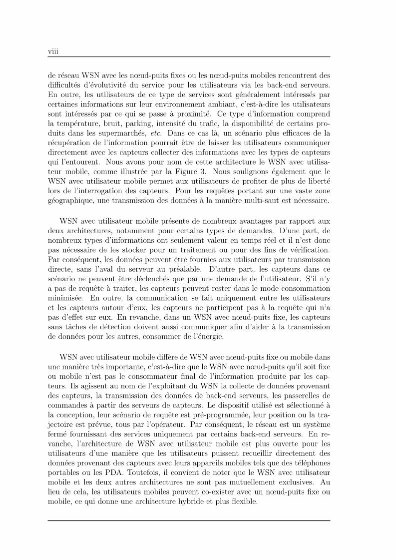
de reseau WSN avec les nœud-puits fixes ou les nœud-puits mobiles rencontrent desdifficultes d’evolutivite du service pour les utilisateurs via les back-end serveurs.En outre, les utilisateurs de ce type de services sont generalement interesses parcertaines informations sur leur environnement ambiant, c’est-a-dire les utilisateurssont interesses par ce qui se passe a proximite. Ce type d’information comprendla temperature, bruit, parking, intensite du trafic, la disponibilite de certains pro-duits dans les supermarches, etc. Dans ce cas la, un scenario plus efficaces de larecuperation de l’information pourrait etre de laisser les utilisateurs communiquerdirectement avec les capteurs collecter des informations avec les types de capteursqui l’entourent. Nous avons pour nom de cette architecture le WSN avec utilisa-teur mobile, comme illustree par la Figure 3. Nous soulignons egalement que leWSN avec utilisateur mobile permet aux utilisateurs de profiter de plus de libertelors de l’interrogation des capteurs. Pour les requetes portant sur une vaste zonegeographique, une transmission des donnees a la maniere multi-saut est necessaire.

WSN avec utilisateur mobile presente de nombreux avantages par rapport auxdeux architectures, notamment pour certains types de demandes. D’une part, denombreux types d’informations ont seulement valeur en temps reel et il n’est doncpas necessaire de les stocker pour un traitement ou pour des fins de verification.Par consequent, les donnees peuvent etre fournies aux utilisateurs par transmissiondirecte, sans l’aval du serveur au prealable. D’autre part, les capteurs dans cescenario ne peuvent etre declenches que par une demande de l’utilisateur. S’il n’ya pas de requete a traiter, les capteurs peuvent rester dans le mode consommationminimisee. En outre, la communication se fait uniquement entre les utilisateurset les capteurs autour d’eux, les capteurs ne participent pas a la requete qui n’apas d’effet sur eux. En revanche, dans un WSN avec nœud-puits fixe, les capteurssans taches de detection doivent aussi communiquer afin d’aider a la transmissionde donnees pour les autres, consommer de l’energie.

WSN avec utilisateur mobile differe de WSN avec nœud-puits fixe ou mobile dansune maniere tres importante, c’est-a-dire que le WSN avec nœud-puits qu’il soit fixeou mobile n’est pas le consommateur final de l’information produite par les cap-teurs. Ils agissent au nom de l’exploitant du WSN la collecte de donnees provenantdes capteurs, la transmission des donnees de back-end serveurs, les passerelles decommandes a partir des serveurs de capteurs. Le dispositif utilise est selectionne ala conception, leur scenario de requete est pre-programmee, leur position ou la tra-jectoire est prevue, tous par l’operateur. Par consequent, le reseau est un systemeferme fournissant des services uniquement par certains back-end serveurs. En re-vanche, l’architecture de WSN avec utilisateur mobile est plus ouverte pour lesutilisateurs d’une maniere que les utilisateurs puissent recueillir directement desdonnees provenant des capteurs avec leurs appareils mobiles tels que des telephonesportables ou les PDA. Toutefois, il convient de noter que le WSN avec utilisateurmobile et les deux autres architectures ne sont pas mutuellement exclusives. Aulieu de cela, les utilisateurs mobiles peuvent co-exister avec un nœud-puits fixe oumobile, ce qui donne une architecture hybride et plus flexible.

ix

Motivations et objectifs Cette these a ete motivee par la collecte d’informationin-site appliquees a des applications du service public a grande echelle. Nous noussommes interesses en particulier a l’architecture de WSN avec utilisateur mobile. Cesapplications presentent de plus en plus d’interets a la fois industriels et academiques.Une architecture a plusieurs nœud-puits de mobile a ete proposee dans [CM06]. Danscette architecture, les telephones cellulaires sont equipes de plusieurs interfaces sansfil: un reseau de base de communication mobile et l’autre pour communiquer avecd’autres peripheriques via les connexions sans fil courte distance, tels que Bluetoothet ZigBee. Sur la base de ces telephones cellulaires multi-radio, il est possible defournir des services de WSN utiles pour le grand public. Nous soulignons ici plusieursd’entre eux avec seulement leurs scenarios de base et les caracteristiques distinctes.

• Systeme d’information Omnipresent: Capteurs sans fil peuvent etre deployesle long des rues de la ville et les parkings afin que les pilotes puissent accedera l’information en temps reel sur le trafic a venir et les parkings disponiblesa proximite avec leurs telephones cellulaires. Apparemment, on se soucie plusgeneralement des informations de trafic sur une petite region, ou d’informationdu parking autour de la destination.

• Systeme Contre-Emergence: Un autre domaine d’application pour un WSNavec utilisateur mobile peut etre le recueil d’information pendent des operationsd’emergence. Nœuds de capteurs sans fil peuvent etre deployees a l’interieuret autour d’un feu afin de faciliter l’operation. Avec certains dispositifs porta-bles, les pompiers sont en mesure de recueillir diverses informations provenantde capteurs qui les entourent, afin de prendre des bonnes actions afin qu’ellespuissent se tenir a l’ecoute des explosions dangereuses, eviter d’etre pris aupiege ou a localiser les victimes.

Nous insistons sur plusieurs caracteristiques de ces types d’applications et leWSN avec utilisateur mobile ci-dessous:

• Le reseau de capteurs sans fil dans ce cas est plus oriente vers l’utilisateurque les applications militaires ou scientifiques. Pour le systeme d’informationomnipresent mentionne ci-dessus, les utilisateurs ont acces aux services par uncontrat, devenant ainsi les clients du reseau. En consequence, il est necessaireque les fournisseurs de services satisfont leurs clients. Pour les systemes contre-urgence, satisfaire les besoins fondamentaux de chaque agent est importantmeme s’il est plus probable qu’ils appartiennent a la meme organisation.

• Les utilisateurs ne sont pas geres par les operateurs du reseau. S’il est vraique les appareils en service doivent repondre a certains besoins fonctionnels,certains contrats entre les utilisateurs et l’operateur sont necessaires, les profilsutilisateur, tels que des mode d’acces, la position, etc. ne peuvent pas etrecontroles par l’operateur.

• Les utilisateurs sont autonomes et ils n’ont generalement pas de contact directles uns avec les autres. Au contraire, ils sont habituellement en concurrenceles uns avec les autres pour les ressources du reseau.

x

En vertu d’un tel environnement autonome, avec la contrainte de ressourcesstricte, de multiples utilisateurs doivent partager les ressources communes de manieresatisfaisante en vue d’exploiter le reseau dans un etat optimal en fonction de la pop-ulation d’utilisateurs et de la repartition geographique. En particulier, on voudraitempecher que certains utilisateurs soient bloques parce qu’ils entrent dans le reseauapres que les autres utilisateurs ont consomme toutes les ressources disponibles.Cela exige d’enqueter sur une serie de problemes d’optimisation, qui sont au centredes preoccupations de cette these.

Cette these vise les problemes d’optimisation de reseau de l’origine du WSNavec utilisateur mobile defini precedemment. Les problemes seront elabores avec laprogrammation mathematique et resolues de maniere analytique et algorithmique.Deux objectifs d’optimisation seront etudies, l’un est de maximiser la satisfaction detous les utilisateurs dans le reseau et l’autre est de donner a chaque utilisateur unepartie equitable du service fourni par le reseau. Les deux objectifs d’optimisationsoulignent davantage le cote utilisateur. Ce point de vue est considere comme l’unedes nouveautes de cette these. Lorsque le WSN doit fournir les services a ses clients,d’optimiser des parametres au cote client, par exemple, leur gamme de requete,est tout a fait logique. En consequence, les parametres au cote capteur qui sontconsideres comme critiques dans la litterature courante, comme l’efficacite de laconsommation d’energie et de la duree de vie du reseau, sont d’importance sec-ondaire dans cette these. Nous estimons que la limite des ressources sur le capteurseulement comme des contraintes dans la formulation des problemes d’optimisation.La ressource en cours d’examen est la bande passante effective du capteur.

De toute evidence, pour une architecture de reseau, tels que le WSN avec util-isateur mobile que nous etudions, toute solution doit etre capable de s’adapter a ladynamique de reseau. Par exemple, un utilisateur rejoint ou quitte, le changementde sa position, la quantite d’information il requit, etc. Cela exige essentiellement unesolution distribuee qui permet la cooperation entre les utilisateurs et les capteursa la realisation de certains objectifs d’optimisation. Par consequent, cette these seconcentrera principalement sur la formulation des problemes d’optimisation et lessolutions distribuees.

En resume, cette these a pour objectif de proposer des algorithmes distribuespour les utilisateurs et les capteurs dans un WSN afin d’allouer un rayon optimalde requete pour chaque utilisateur de facon adaptative et evolutive.

Allocation de Requete dans un WSN avec Utilisateur Mobile

Dans certains application contre-emergence, le reseau de capteur sans fil pour-rait considerablement aider les equipes d’intervention par notification a certainsevenements. Une application typique de ce reseau pourrait etre un systeme desurveillance avec des pompiers equipes de dispositifs portables qui collectent lesdonnees a partir d’une zone de combustion afin de determiner un perimetre desecurite, tandis que d’autres operent sur le foyer et sont en alerte en temps reel surles risques d’explosions a proximite. Les pompiers ont envoye des demandes pourrecueillir des donnees provenant des capteurs a l’interieur d’un domaine specifique.

xi

Ainsi, ils pourraient etre consideres comme les utilisateurs mobiles.Ce systeme de surveillance doit etre digne de confiance, afin que tous les evenements

dans une zone controlee doivent etre signales a l’utilisateur d’interrogation, et de-vraient etre adaptables, puisqu’il y a des changements de nombre d’utilisateurs aufil du temps. En outre, il est souhaite pour chaque utilisateur de controler la plusgrande zone possible pour assurer la securite individuelle. Toutefois, etant donneque le nœud de capteur a une bande passante limitee, de multiples requetes pour-raient congestionner les capteurs dans certaines zones, en fonction de la positiondes utilisateurs, la taille de la zone, etc. En outre, si les capteurs sont deja saturespar les requetes, les utilisateurs recemment arrives seront conserves dans un etatde faim et de l’impossibilite de recuperer les informations. Au contraire, si chaquepompier accepte de diminuer la taille de sa zone de requete, cela peut permettre auxnouveaux venus d’utiliser le reseau. Ainsi, l’equite entre les utilisateurs partageantle reseau est preferable. En consequence, les utilisateurs ont tendance a augmenterleurs rayons de requete tant que des regles d’equite sont conserves. Nous supposonsque les utilisateurs ne sont pas coordonnes par les liens de communication directs.

Un Modele de Requete Continu

Une requete emise par un utilisateur appartient a une zone supposee etre un disquede rayon variable centre sur l’utilisateur. Chaque capteur a l’interieur de la zonea demande de generer certaines quantite de donnees par seconde en reponse a larequete. Un capteur peut etre couvert par plusieurs requetes.

Le modele de la charge de trafic que nous utiliserons a ete propose dans [GK04]et etendu dans [LH05]. Avec ce modele de trafic, nous sommes en mesure d’obtenirune representation analytique du trafic genere par un capteur de n’importe quelleposition dans le reseau. C’est une fonction de la position du nœud et de l’utilisateurqui interroge le capteur, ainsi que d’autres parametres, montre comme suit:

δ(dki) =

br2

(r∗)2 k ∈ r∗ib+ 2br2

π(r∗)2 arcsin(r∗dki

)− 2bd2ki

π(r∗)2 arcsin(r∗dki

)k ∈ Qrib \ r∗i

0 otherwise

(1)

ou r∗ signifie la distance maximum de transmission d’un capteur, r∗i signifie la disquede rayon r∗ centree au capteur i et Qrib signifie la region couverte par la requete derayon ri d’utilisateur i avec b comme le trafic demande sur chaque capteur.

Configuration Equite Max-min: Une configuration est definie par un ensemblede paire rayon-utilisateur: C = (ri|i ∈ S) et nous disons que C est une configurationfaisable s’il n’y a pas de congestion dans le reseau. Nous nous sommes interesses al’equite max-min, c’est a dire que C possede des proprietes telles que les rayons pluspetits sont maximises, les rayons deuxiemes plus petits sont maximises et ainsi desuite. Une regle de base est que l’augmentation d’une requete ne devrait pas dimin-uer d’autres requetes deja plus petits. De toute evidence, la limite de la capacitedoit etre maintenue. Notez que dans le contexte que nous examinons, le trafic b estfixe et chaque utilisateur s’est interesse a maximiser son rayon de requete afin demaximiser la securite individuelle.

xii

Un Modele de Requete Discrete

La requete est mesuree par le nombre de sauts tels qu’une requete de rayon j couvretous voisins de j sauts de l’utilisateur.

Nous avons suppose que tous les nœuds inclus dans la requete de l’utilisateurdoivent fournir une certaine quantite de ressources. Notez que si un nœud k est dansune requete, alors tous les nœuds le long du chemin de transmission de donnees sontdans la meme requete et ils consomment des ressources en transmettant les donnees apartir de k. Comme nous avons egalement assume qu’un mecanisme de routage avecles chemins plus courts est en cours d’utilisation, le montant de ressource des nœudsle long de la route doit fournir, en raison de l’impact de l’utilisateur i, est egal ousuperieur a ce que le nœud k doit fournir, si le flux de donnees est vers l’utilisateur.A noter que nous supposons qu’il n’y a pas de compression ou d’agregation desdonnees sur les chemins.

Chaque nœud k admet des ressources quantifiables comme ck qu’il est en mesurede fournir a certains utilisateurs. Le montant de ressource sur le nœud k quel’utilisateur i consomme lorsque son rayon de requete est fixe a j est designee commewijk. Si le nœud i n’appartient pas a Vjib, nous avons wijk = 0.

Nous n’utilisons pas la fonction de trafic pour cette etude. Au lieu de cela, nousallons mettre en place des mecanismes pour chaque nœud pour mesurer le traficreel.

Nous definissons l’allocation de requete avec equite max-min (MMF) de la mememaniere que nous l’avons fait pour le modele continu. Par ailleurs, nous definissonsegalement un autre objectif d’optimisation afin de maximiser la somme des rayonsde requetes de tous les utilisateurs (MNU).

Nous modelisons le probleme avec un probleme sac a dos. Chaque requeted’utilisateurs i correspond a un element a etre selectionne et la valeur des elementspourrait etre le nombre de saut de 0 au diametre de G note DG. Etant donneque chaque utilisateur est autorise a choisir une seule valeur pour sa requete a lafois, les elements peuvent etre consideres comme regroupes en m classes et chaqueclasse correspond a un utilisateur. Ainsi, nous avons la contrainte de choix mul-tiples que exactement un element doit etre choisi au sein de chaque classe. Unevariable binaire xij est associee a la gamme de requete j de l’utilisateur i ou xij = 1indique que l’utilisateur i definit ses requete gamme j, et xij = 0 autrement. Lemontant des ressources fournies par un nœud k a un utilisateur i quand i prendchacune de ses requetes possible j ∈ (0, 1, . . . , DG) sera considere comme un ensem-ble (wi0k, wi1k, . . . , widGk), et chaque wijk pourrait etre associe a la ieme dimensiondu poids d’un element j de la classe i. Chaque nœud k forme une dimension decontrainte avec ses ressources disponibles ck. Comme il y a beaucoup de nœudsdans le systeme, nous avons enfin une contrainte multi-dimensionnelle, c’est-a-dire,un MMKP. Le probleme d’allocation de requete discret de maximiser la somme del’utilite de chaque utilisateur, est exactement le classique MMKP. Il pourrait etreresolu par des algorithmes MMKP. Cependant, tous ces algorithmes examinent laresolution du probleme dans un mode central. Etant donne la nature des problemesqui ont motive ce travail, un algorithme distribue est preferable. Nous allons pro-

xiii

poser un tel algorithme. En outre, nous avons egalement formule le probleme MMKPavec l’equite max-min. Cet objectif est nouveau et interessant car il demontre lapossibilite de formuler differents objectifs d’optimisation dans un cadre de MMKP.

Solution du Modele Continu

Calculer le rayon d’equite max-min. Si la requete prend une valeur continue,nous sommes en mesure de le calculer en fonction de l’equite max-min dans unreseau avec seulement deux utilisateurs. Nous considerons que deux utilisateurs dei et i′ sont dans le reseau.

Dans un WSN avec des nœuds a la distribution Poisson et un paradigme con-vergent de communication, le goulot est l’utilisateur lui-meme [MDMLN03]. Nousdisons que la requete est globalement maximisee quand la bande passante de tousles nœuds dans les ri est saturee par le trafic exclusivement dedie a i. Si on faitabstraction de la bande passante consommee par le protocole, la requete est glob-alement maximisee quand πriλ0b = W . Lorsque le debit de donnees demande (b) etla densite de capteurs (λ0) sont fixes, nous allons naturellement obtenir:

rmax =

√W

πbλ0

(2)

Dans ce cas, le montant maximum de donnees qu’un utilisateur peut recevoirest limite par sa bande passante et les deux requetes pourraient etre maximiseesavec la meme rayon rmax. De toute evidence, la configuration C = (ri, ri′) avecri = ri′ = rmax est max-min equite. On peut obtenir les memes resultats pour lescas suivants.

Deux utilisateurs pas si lointains: Dans ce cas la, deux utilisateurs peuvent fixerles requetes a rc et chaque utilisateur peut determiner rc en communiquant avec uncapteur de sa requete. Ainsi, la configuration max-min pour ce cas est C = (ri, ri′)ou ri = ri′ = rc, et:

rc =

√√√√( Wπ(r∗)2λ0

− b+ t1

)t2

, (3)

ou:

t1 =2b(d− r∗)2

π(r∗)2arcsin

(r∗

d− r∗

)(4)

t2 =b

(r∗)2+

2b

π(r∗)2arcsin

(r∗

d− r∗

)(5)

Deux utilisateurs a proximite: La configuration max-min est C = (ri, ri′) avec

rc =

√W

2πλ0b. (6)

Ca complete l’analyse de la configuration max-min pour le cas de deux utilisateurs.

xiv

Un algorithme distribue L’algorithme se compose de deux phases. Le premier,generalement appele demarrage lent, est utilisee jusqu’a ce qu’une approximationd’un rayon realisable est obtenue. Le rayon commence a une valeur unitaire etaugmente selon une certaine strategie jusqu’a ce que l’utilisateur soit prevenu parun message <saturated>. La fonction initRadius gere l’augmentation initiale derayon. Le initRadius est fonde sur une croissance exponentielle, c’est-a-dire lerayon de requete est initialise a 1 et double a chaque fois qu’il est appele. L’idee estde detecter le plus rapidement possible le goulot d’etranglement de capteurs.

A la reception du premier message <saturated>, le rayon est fixe a une valeurplus basse en fonction de certains criteres. Le nouveau rayon est obtenu par resetRadius.Le resetRadius emploie le resultat d’analyse pour les deux utilisateurs presentesci-dessus, et la fonction retourne un rayon proche de la solution optimale dans laplupart des cas. Dans la deuxieme phase, chaque utilisateur essaie d’augmenterson rayon de requete periodiquement, afin d’explorer le rayon optimal. Ceci estpris en charge par la fonction increaseRadius. Le increaseRadius fait une fonc-tion croissante lineaire du rayon apres chaque intervalle de temps predefini par uneetape de longueur predefinie. Finalement, l’utilisateur est prevenu par un message<saturated>, puis il diminue a nouveau son rayon et entre dans un nouveau cycle.

Solution du Modele Discrete

L’idee de base des algorithmes est de resoudre un probleme localise beaucoup pluspetit a chaque nœud. A cette fin, chaque nœud garde la trace de tout le trafic passantpar lui-meme. Avec cette information, quand un nœud est sature par plusieursrequetes d’utilisateurs, il est en mesure de formuler un MMKP locale avec seulementles utilisateurs concernant et une unique contrainte. Ce probleme est generalementbeaucoup plus petit et pourrait etre resolu rapidement. Puis le nœud avertit lesutilisateurs en relation avec la solution. Eventuellement, l’utilisateur adopte unedes solutions multiples en tant que son nouveau rayon de requete. Dans le restede cette section, nous donnons d’abord des discussions detaillees sur les techniquescles que nous emploierons, puis nous proposons un algorithme unifie pour les deuxobjectifs d’optimisation MMF et MNU.

Solution du MCKP Local

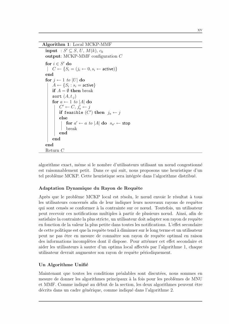
Lorsque le nœud est sature, il formule un petit probleme MMKP avec ses mesuresdu trafic local et une seule contrainte, ou de maniere equivalente, un problemeMCKP. Ce MCKP doit etre resolu d’une maniere centralisee ainsi des algorithmesexacts ou heuristiques peuvent etre exploites. Divers algorithmes ont ete proposespour resoudre un MCKP avec l’objectif de maximisation de la somme d’utilite detous les utilisateurs. Nous adoptons un outil GLPK pour resoudre ce problemeMCKP dans le cadre d’un algorithme distribue que nous allons proposer pour leprobleme de MNU. En revanche, aucun algorithme n’a ete propose pour un MCKPavec l’objectif MMF. Depuis que le MCKP est un cas particulier de MMKP, ilest possible d’appliquer directement l’algorithme exact que nous allons proposer aresoudre ce MCKP. Toutefois, le cout de calcul augmente de facon exponentielle d’un

xv

Algorithm 1: Local MCKP-MMF

input : S ′ ⊆ S, U , M(k), ckoutput: MCKP-MMF configuration C

for i ∈ S ′ doC ← {Si = (ji ← 0, si ← active)}

endfor j ← 1 to |U | do

A← {Si : si = active}if A = ∅ then breaksort (A, t·j)for a← 1 to |A| do

C ′ ← C, j′a ← jif feasible (C ′) then ja ← jelse

for a′ ← a to |A| do sa′ ← stopbreak

end

end

endReturn C

algorithme exact, meme si le nombre d’utilisateurs utilisant un nœud congestionneest raisonnablement petit. Dans ce qui suit, nous proposons une heuristique d’untel probleme MCKP. Cette heuristique sera integree dans l’algorithme distribue.

Adaptation Dynamique du Rayon de Requete

Apres que le probleme MCKP local est resolu, le nœud envoie le resultat a tousles utilisateurs concernes afin de leur indiquer leurs nouveaux rayons de requetesqui sont censes se conformer a la contrainte sur ce nœud. Toutefois, un utilisateurpeut recevoir ces notifications multiples a partir de plusieurs nœud. Ainsi, afin desatisfaire la contrainte la plus stricte, un utilisateur doit adapter son rayon de requeteen fonction de la valeur la plus petite dans toutes les notifications. L’effet secondairede cette politique est que la requete tend a diminuer sur le long terme et un utilisateurpeut ne pas etre en mesure de connaıtre son rayon de requete optimal en raisondes informations incompletes dont il dispose. Pour attenuer cet effet secondaire etaider les utilisateurs a sauter d’un optima local affectes par l’algorithme 1, chaqueutilisateur devrait augmenter son rayon de requete periodiquement.

Un Algorithme Unifie

Maintenant que toutes les conditions prealables sont discutees, nous sommes enmesure de donner les algorithmes principaux a la fois pour les problemes de MNUet MMF. Comme indique au debut de la section, les deux algorithmes peuvent etredecrits dans un cadre generique, comme indique dans l’algorithme 2.

xvi

Algorithm 2: Distributed Heuristic

Sink Part : Run at user isend < level, i, 1 >while no < adjust-level > message do

level← initLevel()

send < level, i, level >endlevel← adjustLevel()

while true dowhile no < adjust-level > message do

level← increaseLevel()

send < modify-level, i, level >endlevel← adjustLevel()

send < modify-level, i, level >end

Sensor Part: Run at sensor kwhile true do

if congested() thenC ← solveMCKP()

for ∀i : ji ∈ C dosend < adjust-level, ji > to i;

end

end

end

Le Probleme Derriere: Instance Difficile du MMKP

Nous avons formule la version discrete du probleme d’allocation de requete pourun WSN avec utilisateur mobile avec un probleme sac a dos multidimensionnel auxchoix multiples. Nous nous concentrons maintenant sur ce probleme combinatoirelui-meme.

MMKP a de nombreuses applications. Il a ete utilise pour modeliser le problemede gestion de la qualite de service (QoS) dans les reseaux informatiques [LLRS99] etles problemes de controle adaptatif d’admission dans le systemes multimedia [SIH05,Kha98, KLMA02]. Divers autres problemes d’allocation des ressources peuventegalement etre directement representes par le MMKP [KPP04, PHD05].

Nous etudions la relation entre les differents parametres d’un MMKP telles quele profit, le poids et la capacite afin d’identifier les facteurs cles qui rendent uneinstance difficile. En outre, les cas ou les elements sont non correles, faiblementcorreles et fortement correles au sein de chaque classe, entre les classes et a traversde multiples dimensions sont examines. A notre connaissance, aucun travail n’a etesignale dans la litterature. Une methode systematique pour generer les instances deMMKP est proposee. Plusieurs groupes de cas obtenues avec cette methode sont

xvii

evalues avec un algorithme exact et les outils GLPK [glp] et CPLEX [cpl]. Lesexperiences montrent que de nombreux cas sont de plusieurs ordres de grandeurplus difficiles que ceux traditionnellement utilises en terme de temps de calcul. Cesinstances dures du MMKP ont generalement une capacite moyenne et une fortecorrelation entre le poids et le profit. Les experiences suggerent egalement que lescas avec les profits similaires entre les classes et avec une forte correlation entre lepoids et le profit sont difficiles a resoudre.

Noter qu’il est tres important de tester les algorithmes afin de connaıtre leursperformances en pratique. Lorsque les algorithmes sont pour attaquer a un problemeparticulier, les instances ideales pour l’evaluation des performances sont ceux detraces du monde reel. Toutefois, comme les MMKPs proviennent habituellement descontextes applicatifs diversifies, les instances typiques a partir d’un certain domainene peuvent guere etre raisonnables pour les autres. En outre, il n’existe pas derapport systematique sur les instances de MMKP dans la litterature. En revanche,les cas de test peuvent etre generes pour couvrir les instances de type d’une gammebeaucoup plus large. En consequence, les instances generees jouent un role importantdans l’evaluation comparative des algorithmes et ont ete utilisees dans les recherchesde KP et MMKP.

Les chercheurs ont propose une librairie des instances de MMKP [OR-]. Bien queces instances ont ete largement utilisees dans la litterature, nos resultats de calculmontrent qu’ils ne sont pas suffisants pour demontrer les performances des algo-rithmes. Table 1 presente le temps utilise pour resoudre les six premieres instancesdans la librairie avec CPLEX, GLPK et l’algorithme BBLP [Kha98, KLMA02]. Ici,nous insistons sur le temps utilise a travers les instances. Notamment, les instancesI3 et I4 prennent plus de temps que I5 et I6, malgre qu’ils soient plus petits queles seconds. Cela implique effectivement que non seulement la taille d’une instance,mais aussi la structure d’une instance joue un role tres important dans le temps deresolution.

Table 1: Temps (second) utilise pour resoudre les instances dans “OR benchmarklibrary”.

Inst m n l CPLEX GLPK BBLPI1 5 5 5 0.005 0.028 0.016I2 10 5 5 0.006 0.029 0.033I3 15 10 10 1.983 16.036 67.260I4 20 10 10 31.045 1383.251 1532.059I5 25 10 10 0.018 0.046 0.660I6 30 10 10 0.204 0.190 2.369

xviii

Nouvelles Methodes pour Generer les Instances de

MMKP

Generer les Profits

Afin de selectionner les profits des elements dans chaque classe i, nous avons d’abordlimite les profits avec deux parametres pmin

i et pmaxi et choisi des valeurs dans cette

intervalle. Cela pourrait se faire de diverses manieres et ici, nous definissons quelquesfonctions generatrices pour les profits.

Fonction Generatrice Uniforme Profits aleatoires sont naturelles dans de nom-breux problemes et sont largement utilises dans la litterature. Dans une fonctiongeneratrice uniforme, nous tirons les profits de maniere uniforme et aleatoire dansun intervalle. On note la fonction generatrice uniforme:

pij = U(pmini , pmax

i

). (7)

Fonction Generatrice Lineaire Elements avec les profits lineaires sont moinsetudies dans la litterature. Toutefois, ce type de valeur est en fait assez com-mun. Par exemple, dans le probleme de QoS adaptative [AHHS05], les niveauxde qualite de service sont habituellement representes sur les profits d’elements etde valeurs entieres consecutives. Aussi dans le probleme d’allocation de requetemulti-sauts [HLS09], les rayons de requetes sont mis en correspondance avec lesprofits et se mesurent en nombre de sauts et ils prennent aussi des valeurs entieresconsecutives.

Dans la fonction generatrice lineaire, nous assignons pij avec une fonction lineairede l’indice j, i.e.

pij =j − 1

ni − 1

(pmaxi − pmin

i

)+ pmin

i . (8)

Pour plus de clarte, nous utilisons une notation courte pour cette fonction generatricelineaire comme suit:

pij = L(pmini , pmax

i

). (9)

Application des Fonctions Generatrices Les fonctions generatrices doiventetre appliquees sur chaque classe. Evidemment, on peut appliquer la meme fonc-tion pour toutes les classes ou modifier les fonctions de chaque classe. Pour unefonction generatrice uniforme, meme quand elle est appliquee a toutes les classesavec les memes parametres, la nature aleatoire de la fonction va donner differentesvaleurs pour les profits dans les differentes classes. Au contraire, lorsque la fonctiongeneratrice lineaire est appliquee a toutes les classes avec les memes parametres,toutes les classes auront le meme vecteur de profit pour leurs elements. Au lieud’appliquer la meme fonction generatrice a toutes les classes, nous proposons enoutre deux facons d’utiliser les fonctions generatrices. La premiere est de repro-duire le vecteur genere par une fonction generatrice uniforme sur toutes les classes.

xix

C’est typiquement le cas lorsque plusieurs utilisateurs (classes) peuvent acceder auxmemes ensembles d’objets (elements) avec plus ou moins de qualite du service (prof-its), mais le cout pour y acceder differe (poids). On designe explicitement les profitsgeneres par cette maniere:

pij = R(U(pmin

1 , pmax1

)). (10)

Ici, R signifie Reproduire le premier vecteur de profit genere pour d’autres classes.La deuxieme facon d’appliquer les fonctions de production est de prendre en comptel’indice de classe i au moment de decider de l’intervalle a partir de laquelle les valeurssont prises pour chaque classe, e.g. U(10(i−1), 10i) ou L(10(i−1), 10i). Lorsque lafonction generatrice uniforme est appliquee de cette facon, les profits dans chaqueclasse sont toujours choisis aleatoirement, mais les profits des differentes classessont disperses dans differents intervalles. Bien que la fonction generatrice lineaireest appliquee, les profits sont lineairement attribues a des intervalles differents. Onnote cette application particuliere des fonctions generatrices comme:

pij = C(F ), (11)

ou F est une fonction generatrice avec des parametres differents pour differentesclasses et C signifie que la fonction est dependante d’un classe.

Generer les Poids

Pour generer les poids, on peut appliquer une certaine correlation sur la fonctiongeneratrice pour chaque dimension. En particulier, nous definissons les fonctionsgeneratrices suivantes.

Fonction Generatrice Non-Correlee Dans une fonction generatrice non-correlee,nous attribuons simplement les poids de maniere uniforme et aleatoire dans un in-tervalle:

wijk = U(wminik , wmax

ik

). (12)

Fonction Generatrice Faiblement Correlee Cette fonction generatrice est mo-tivee par des resultats sur les instances du KP [Pis05]. La motivation est de genererles poids correles aux profits, mais toujours avec un degre de liberte pour chaquedimension. Dans notre proposition, les poids sont attribuees en fonction de:

wijk = U(

max

(0, pij −

pmaxi

δ

), pij +

pmaxi

δ

). (13)

Nous allons utiliser la notation suivante:

wijk =W(δ). (14)

xx

Fonction Generatrice Fortement Correlee Fonction generatrice fortementcorrelee est egalement motivee par les resultats precedents ou la correlation entreles profits et les poids est forte:

wijk = pij +pmaxi

δ. (15)

Nous utilisons la notation suivante pour cette fonction:

wijk = S(δ). (16)

Fonction Generatrice Fortement Inversee Correlee Pour une fonction generatricefortement inversee correlee, les poids sont attribuees en fonction de:

wijk = pmaxi − pij

δ, (17)

et sera denommee:

wijk = I(δ). (18)

Notez que la fonction generatrice fortement inversee correlee n’est pas interessantepour etre utilise seule. Les cas interessants se produisent lorsque les deux fonctions,fortement correlee et fortement inversee correlee coexistent sur les differentes dimen-sions de poids. Intuitivement, ces cas sont difficiles a resoudre parce qu’un choixattentif entre les poids a travers plusieurs dimensions doit etre fait. Bien que nousn’avons pas de connaissance de problemes realistes de ce type de MMKP, ils sontencore interessants d’un point de vue theorique.

Application des Fonctions Generatrices Similaires aux fonctions generatricespour les profits, on pourrait appliquer la meme fonction generatrice avec les memesparametres a toutes les dimensions. Mais il est egalement possible d’appliquer lameme fonction avec des parametres differents ou meme des fonctions differentes pourles dimensions. En plus d’appliquer simplement la meme fonction generatrice avecles memes parametres sur toutes les dimensions, ici nous vous proposons deux faconsd’appliquer les fonctions generatrices pour les poids. Le premier est d’inclure l’indicede dimension k comme un parametre dans la fonction generatrice. Par exemple,pour une fonction generatrice non-correlee, les poids d’une dimension k peuventetre choisis dans un intervalle qui depend de k, ou pour une fonction faiblement,fortement et fortement inversee correlee, le parametre δ peut etre choisi en fonctionde k. Il est commode d’utiliser une notation comme suit:

wijk = D(F ), (19)

ou F peut etre, par exemple, U(1, 10k) pour une fonction generatrice uniforme, ouW(k + 5) et S(k + 5) pour une fonction generatrice faiblement correlee et forte-ment correlee, respectivement. Ici, D, signifie que les fonctions generatrices sontDimension-dependantes. Nous pourrions egalement appliquer differentes fonctions

xxi

generatrices pour differentes dimensions. Par exemple, nous allons generer des in-stances avec la fonction generatrice fortement inversee correlee pour quelques di-mensions et la fonction generatrice fortement correlee pour les autres. Dans ce cas,on note:

wijk = D(F1F2 . . . ), (20)

ou F1, F2, . . . sont les fonctions generatrices que nous utilisons.

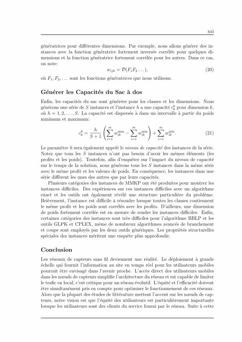
Generer les Capacites du Sac a dos

Enfin, les capacites du sac sont generees pour les classes et les dimensions. Nousgenerons une serie de S instances et l’instance h a une capacite chk pour dimension k,ou h = 1, 2, . . . , S. La capacite est dispersee a dans un intervalle a partir du poidsminimum et maximum:

chk =h

S + 1

(m∑i=1

wmaxik −

m∑i=1

wminik

)+

m∑i=1

wminik . (21)

Le parametre h sera egalement appele le niveau de capacite des instances de la serie.Notez que tous les S instances n’ont pas besoin d’avoir les memes elements (lesprofits et les poids). Toutefois, afin d’enqueter sur l’impact du niveau de capacitesur le temps de la solution, nous generons tous les S instances dans la meme serieavec le meme profit et les valeurs de poids. En consequence, les instances dans uneserie different les unes des autres que par leurs capacites.

Plusieurs categories des instances de MMKP ont ete produites pour montrer lesinstances difficiles. Des experiences sur ces instances difficiles avec un algorithmeexact et les outils ont egalement revele une structure particuliere du probleme.Brievement, l’instance est difficile a resoudre lorsque toutes les classes contiennentle meme profit et les poids sont correles avec les profits. D’ailleurs, une dimensionde poids fortement correlee est en mesure de rendre les instances difficiles. Enfin,certaines categories des instances sont tres difficiles pour l’algorithme BBLP et lesoutils GLPK et CPLEX, meme de nombreux algorithmes avances de branchementet coupe sont employes par les deux outils generiques. Les proprietes structurellesspeciales des instances meritent une enquete plus approfondie.

Conclusion

Les reseaux de capteurs sans fil deviennent une realite. Le deploiement a grandeechelle qui fournit l’information au site en temps reel pour les utilisateurs mobilespourrait etre envisage dans l’avenir proche. L’acces direct des utilisateurs mobilesdans les nœuds de capteurs simplifie l’architecture du reseau et est capable de limiterle trafic en local, c’est critique pour un reseau evolutif. L’equite et l’efficacite doiventetre simultanement pris en compte pour optimiser le fonctionnement de ces reseaux.Alors que la plupart des etudes de litterature mettent l’accent sur les nœuds de cap-teurs, notre vision est que l’equite des utilisateurs est particulierement importantelorsque les utilisateurs sont des clients du service fourni par le reseau. Suite a cette

xxii

vision, nous etudions des questions d’equite dans le reseau de capteurs sans fil dupoint de vue d’un utilisateur.

Nous avons identifie et etudie le probleme d’allocation equitable des requetespour un WSN avec utilisateur mobile. Plusieurs questions connexes, i.e. la capacitedes reseaux sans fil ad-hoc et des reseaux de capteurs sans fil, la couche MAC etla couche reseau pour les reseaux de capteurs sans fil, les caracteres du problemesac a dos multidimensionnel aux choix multiples et ses algorithmes et les definitionsde l’equite sont brievement etudies. Cette partie de l’etude sondage nous a fourniune bonne connaissance sur la base de laquelle les aspects suivants du probleme del’allocation de requete ont ete etudies.

(i) Le probleme d’allocation de requete a l’equite Max-Min dans un WSN estdefini et discute. L’analyse est basee sur un modele de requete continue et unmodele de trafic. En vertu de ces hypotheses, la region de requete d’un utilisa-teur est limitee par la bande passante des capteurs et des utilisateurs. Ainsi, lesutilisateurs ont a cooperer avec les capteurs pour atteindre les resultats souhaites.L’expression explicite de requete a l’equite max-min, pour le cas ou seulement deuxutilisateurs existent dans le reseau, est derivee. Et le probleme au cas ou plusieursutilisateurs sont dans le reseau est resolu avec un algorithme heuristique distribue.Nos simulations montrent l’efficacite de l’algorithme propose.

(ii) L’allocation equitable des requetes entre les utilisateurs est egalement etudieeavec un modele discret. Dans ce cas, la valeur discrete du rayon de la requete nepromet plus de l’existence d’une solution equitable max-min. Ainsi, l’equite max-min lexicographique doit etre exploitee. Nous avons egalement constate qu’il estcommode de representer le probleme de l’equite max-min lexicographique sur leMMKP. En outre, l’objectif traditionnel de l’optimisation, ce qui maximise la sommede l’utilite de tous les elements dans le sac, pourrait egalement etre utilise pourmaximiser la somme du rayon de requetes des utilisateurs. Sur la base de ces obser-vations, nous proposons une formulation unifiee pour les deux problemes. Cette for-mulation, d’une part, est en mesure de formuler differents problemes d’optimisationde l’origine d’un WSN avec utilisateur mobile, et d’autre part, implique la mise enœuvre d’un algorithme uniforme et simple pour resoudre les deux problemes. Lessimulations ont ete menees pour evaluer la performance de l’algorithme. Differentesproprietes entre les deux objectifs d’optimisation sont discutees.

(iii) Pour que l’etude ci-dessus soit pratiquement significative, nous etudions lafaisabilite de reformuler le probleme et mettre en œuvre nos solutions dans un WSNbase sur IEEE 802.15.4/ZigBee. Le mode d’arbre du ZigBee est envisage en raisonde son efficacite. En outre, l’attribution des adresses et la routage utilisee par l’arbreZigBee nous permettent un calcul plein localise. L’algorithme distribue que nousavons propose est efficace pour approcher de la solution optimale et pour controlerla congestion.

(iv) Le MMKP a ete utilise pour formuler le probleme d’allocation de requetepour un reseau de capteurs sans fil avec utilisateur mobile avec un modele de requetediscrete. De nombreuses experiences ont montre des proprietes particulieres desinstances du MMKP, i.e. le temps utilise pour resoudre des instances peut varierbeaucoup tel que les instances plus petites prennent beaucoup plus de temps que

xxiii

les grandes. Dans la derniere partie de cette these, nous avons etudie cette questionpar experiences. Une methode systematique pour generer les instances MMKP estproposee et plusieurs groupes d’instances qui representent une variete de types decorrelation entre les parametres du probleme sont generes. Ces instances sont testeesavec l’algorithme BBLP ainsi que deux outils d’optimisation, le GLPK et le CPLEX.Les resultats montrent que les profits lineaires et la correlation forte entre le poidset le profit font des instances tres difficiles pour l’algorithme BBLP et les outils,meme si certains mecanismes avances de la programmation en nombre entier sontintegres dans les deux outils.

Limites et Perspectives

L’etude de cette these a ete basee sur la vision que le WSN sera deploye a grandeechelle pour fournir des services en temps reel a de multiples utilisateurs mobiles quisont en mesure d’acceder directement aux nœuds de capteurs. Outre les problemesd’equite etudies dans cette these, il existe plusieurs autres questions discutables decette architecture du reseau tres particuliere.

Applicabilite La premiere question est de savoir si oui ou non le WSN avec util-isateur mobile est avere utile et sera deploye. Depuis les experiences des appli-cations deployees, de nombreux reseaux de capteurs sont d’une taille tres limiteeen ce qui concerne le nombre de nœuds (e.g. une dizaine de nœuds) et la zonegeographique qu’ils couvrent (des centaines de metres carres). D’un point de vuetechnique, les difficultes majeure pour un grand reseau de capteurs sont la connec-tivite et l’evolutivite. Alors que de nombreux chercheurs sont occupes a resoudre cesproblemes, d’autres remettent en question les besoins d’un grand reseau connecte enpermanence. L’argument c’est que de nombreux petits WSN independants reunisensemble seront suffisants pour des services omnipresentes. Avec ce debat a l’esprit,nous trouvons que le WSN avec utilisateur mobile peut satisfaire les deux parties.D’une part, il pourrait s’etendre a un reseau avec un grand nombre de nœuds cou-vrant une zone geographique tres vaste, tandis que d’autre part, il n’a pas besoind’etre entierement connecte comme les utilisateurs mobiles sont toujours en mesurede recuperer des donnees de nœuds de capteurs qui sont suffisamment proches. Enconsequence, nous avons un fort sentiment que le WSN avec utilisateur mobile aumoins offre une voie prometteuse pour de futures applications omnipresentes dedetection.

Reseau ou Service? Une autre question interessante est devrions-nous separer ouintegrer le reseau avec le service? Traditionnellement, les reseaux de capteurs sontresponsables de la collecte des donnees brutes (probablement avec un traitementtres limite dans le reseau), tandis que les donnees sont fournies aux utilisateurs viaun serveur back-end. En consequence, la plupart des recherches sont de l’aspectreseau sans tenir compte des utilisateurs. Nous avons etudie l’aspect d’utilisateursavec des limites du reseau comme des contraintes. Bien que l’architecture WSN avecutilisateur mobile est originale et realisable pour les applications ou la signification

xxiv

des donnees recueillies ont une forte dependance a l’egard spatial et temporel, i.e.les donnees sont significatives pour une courte periode de temps et fortement lieea l’endroit ou les donnees sont recuperees et elles ne doivent pas etre stockes engeneral, il est infaisable pour les scenarios ou les donnees doivent etre conservees.Pour ce dernier cas, neanmoins, il est possible de soutenir les utilisateurs mobilesavec une architecture traditionnelle.

Multicast et Traitement dans Reseaux Notre formulation du probleme etles algorithmes fonctionne avec un routage du plus court chemin ou un routageavec arbre hierarchique et nous ne considerons que le routage unicast avec aucuntraitement dans les reseaux. En realite, beaucoup de routages ou protocoles decollecte de donnees existent et certains ont un mecanisme inherent de l’agregationde donnees afin de reduire le trafic. Pour les protocoles de routage multicast quienvoient une seule copie de donnees vers des destinations multiples, ou des protocolesde routage avec l’agregation dans les reseaux, notre modele n’est plus valide. Enconsequence, un nouveau modele du trafic est necessaire en vertu de cette situationqui pourraient etre interessante pour les travaux futurs.

Bande Passante Variable Nous avons base notre etude sur les resultats theoriquesde la capacite du WSN qui ont leurs propres limites. Notamment, les resultats sontobtenus comme une valeur asymptotique lorsque le nombre de capteurs dans unezone determinee devient infini. En realite, la bande passante effective entre chaquepaire d’emetteur et le recepteur depend de nombreux facteurs, e.g. le regime de lamodulation, la puissance de transmission, l’etat de transmission des paires de prox-imite, le mecanisme d’acces au medium, etc. La formulation actuelle du problemeavec une bande passante constante partagee n’est pas capable de tenir compte deces facteurs. Alors que le modele complexe est necessaire pour gerer plus de details,les solutions actuelles pourraient etre etendues, sans trop d’effort. La mesure pro-posee dans cette these est capable de s’adapter a la dynamique de la bande passante.Etudier la performance des algorithmes d’allocation dynamique de requete sous sit-uation de la bande passante est une autre perspective sur laquelle le travail actuelpourrait etre prolonge.

Mobilite Meme si nous avons beaucoup insiste sur les utilisateurs mobiles, nousn’avons pas aborde les problemes poses par la mobilite dans cette these, i.e. tousles modeles, l’analyse, les algorithmes sont bases sur des capteurs et les utilisateursstatiques. Cela empeche une application directe des mecanismes proposes a desscenarios reels. Pour que cette etude soit plus pratique, nous allons etendre nospropositions a un environnement utilisateur mobile, qui peut ne pas etre triviallorsque la convergence des algorithmes distribues doit etre mise en œuvre.

Securite L’acces direct des utilisateurs mobiles aux nœuds de capteurs peut souleverdes questions de securite. De toute evidence, un contrat de service doit etre executeentre les utilisateurs et l’operateur du reseau. Une authentification simple protegee

xxv

par un mecanisme de cryptage leger doit etre mise en œuvre a la fois pour les cap-teurs et les utilisateurs.

Pourquoi MMKP est Dur? Enfin, compte tenu du probleme MMKP lui-meme,l’etude empirique presentee dans cette these n’est qu’une premiere etape vers lacomprehension de ses proprietes structurelles. Nous avons montre que les profitslineaires et correlation forte entre les profits et les poids font une instance de MMKPdure, des recherches plus approfondies sont necessaires pour dire pourquoi. Bienque l’algorithme exact BBLP et le GLPK et CPLEX sont des outils utilises pourmontrer ces instances difficiles, des experiences supplementaires de ces instances avecles heuristiques existantes peuvent fournir plus d’indices a la question mentionneeci-dessus. Bien que certaines experiences ont deja montre que certaines heuristiquessont parfois tres efficaces pour resoudre des instances difficiles avec des proprietesspeciales, ce sujet merite une etude en profondeur.

xxvi

xxvii

Abstract

A Wireless Sensor Network (WSN) is a wireless network consisting of spatially dis-tributed sensor nodes to gather information from the physical world. The promisingidea of WSN is to build an information gathering, processing and representing sys-tem that connects human with the physical world. Lots of efforts have been madein recent years on both the theoretical and applicative aspects of WSNs and we canexpect that large scale WSN deployment will be possible in the near future. Thisthesis focuses on the large scale WSN which may serve potentially many users in anopen architecture where each user has direct contact with the sensors. We will referto this architecture as the mobile user WSN. Large scale mobile user WSN providesa promising solution to many applications. Multiple users in the network couldact as data collectors working together for a common task or they could also beend users which have no direct contact between each other. In either case, fairnessamong these users is an important issue in practice.

We first investigate the fairness issues with a simple query model. In this model,multiple users query the sensors located within a circled area. The query circleis assumed to have a continuous variable diameter and centered at the queryinguser. Distributed optimization problem with congestion constraints is formulatedand heuristic algorithm is developed to approximate the optimal solution. Next,a similar problem with a discrete query model is further investigated. In the dis-crete query model, the query range is measured by hop numbers. This variationmakes the problem to be combinatorial and NP-hard. Multidimensional multiplechoice knapsack problem is used to model the problem with both lexicographicalmax-min fairness and maximal query cover objectives. Distributed solutions areproposed and their performance are demonstrated by simulations. Since the ZigBeespecification and IEEE 802.15.4 standard are two de facto standards of the wirelesssensor networks, we study our problems for a wireless sensor network based on suchtechnologies. Special properties of the ZigBee cluster tree structure are exploited tokeep the algorithm fully local thus only limited communications are involved in theproposed distributed algorithms. Efficiency of the algorithms are demonstrated byextensive simulations.

While all the subjects discussed so far are related with the fair capacity sharingproblem found in wireless sensor networks with multiple users, the combinatorialproblem behind the discrete version, namely the multidimensional multiple choiceknapsack problem, is very interesting and deserves special research efforts. Theinconsistency of the solution times of instances with similar parameters and the sharpcontrast between hard small problems and easy large problems motivated our furtherinvestigation on the problem itself. By first proposing methods to generate probleminstances with different properties, we try to solve several groups of instances withthe current algorithm/solvers. Special properties that make the instances hard havebeen identified.

xxviii

xxix

Contents

Acknowledgements iii

Resume v

Abstract xxvii

Contents xxxi

List of Figures xxxiv

List of Tables xxxv

1 Introduction 11.1 A Brief History . . . . . . . . . . . . . . . . . . . . . . . . . . . . . . 11.2 WSN Evolution . . . . . . . . . . . . . . . . . . . . . . . . . . . . . . 21.3 Motivations and Objectives . . . . . . . . . . . . . . . . . . . . . . . 61.4 Contributions . . . . . . . . . . . . . . . . . . . . . . . . . . . . . . . 81.5 Thesis Organisation . . . . . . . . . . . . . . . . . . . . . . . . . . . . 9

2 Background Knowledge 132.1 State-of-the-Art Researches on WSN . . . . . . . . . . . . . . . . . . 13

2.1.1 Supporting Mechanisms . . . . . . . . . . . . . . . . . . . . . 142.1.2 Communication Protocols . . . . . . . . . . . . . . . . . . . . 16

2.1.2.1 Physical Layer . . . . . . . . . . . . . . . . . . . . . 162.1.2.2 The Medium Access Control Layer . . . . . . . . . . 172.1.2.3 The Network Layer . . . . . . . . . . . . . . . . . . . 192.1.2.4 The Transport Layer . . . . . . . . . . . . . . . . . . 21

2.2 Capacity of Wireless Sensor Networks . . . . . . . . . . . . . . . . . . 232.3 The Knapsack Problems . . . . . . . . . . . . . . . . . . . . . . . . . 23

2.3.1 Exact Algorithms for MMKP . . . . . . . . . . . . . . . . . . 242.3.2 Heuristic Algorithms for MMKP . . . . . . . . . . . . . . . . . 25

2.3.2.1 Moser’s Heuristic . . . . . . . . . . . . . . . . . . . . 252.3.2.2 The HEU, M-HEU, I-HEU and MVRC Algorithms . 252.3.2.3 Parallel HEU and Multiprocessor M-HEU . . . . . . 262.3.2.4 The CP and CCP Algorithms . . . . . . . . . . . . . 272.3.2.5 The Der Algo, RLS, MRLS and Other Variations . . 27

xxx CONTENTS

2.3.2.6 The HMMKP Algorithm . . . . . . . . . . . . . . . . 28

2.3.2.7 The C-HEU Algorithm . . . . . . . . . . . . . . . . . 28

2.3.2.8 The CGBA Algorithm . . . . . . . . . . . . . . . . . 29

2.3.3 Summary . . . . . . . . . . . . . . . . . . . . . . . . . . . . . 30

2.4 Fairness . . . . . . . . . . . . . . . . . . . . . . . . . . . . . . . . . . 31

2.4.1 Max-min and Lexicographical Max-min Fairness . . . . . . . . 31

2.4.2 Proportional Fairness . . . . . . . . . . . . . . . . . . . . . . . 31

2.4.3 (p, α)−proportional Fairness . . . . . . . . . . . . . . . . . . . 32

3 Continuous Query Model 33

3.1 Introduction . . . . . . . . . . . . . . . . . . . . . . . . . . . . . . . . 33

3.2 Continuous Query Model . . . . . . . . . . . . . . . . . . . . . . . . . 34

3.3 Analysis of Two-user Case . . . . . . . . . . . . . . . . . . . . . . . . 36

3.4 Distributed Algorithms . . . . . . . . . . . . . . . . . . . . . . . . . . 38

3.4.1 Brute force algorithm . . . . . . . . . . . . . . . . . . . . . . . 38

3.4.2 Inspiration from two-user case . . . . . . . . . . . . . . . . . . 39

3.4.3 Distributed algorithm and protocol . . . . . . . . . . . . . . . 41

3.5 Performance Evaluation . . . . . . . . . . . . . . . . . . . . . . . . . 43

3.6 Related Works . . . . . . . . . . . . . . . . . . . . . . . . . . . . . . . 48

3.7 Summary . . . . . . . . . . . . . . . . . . . . . . . . . . . . . . . . . 48

4 Reformulating The Problem: A Discrete Query Model 51

4.1 Model and Problem Formulation . . . . . . . . . . . . . . . . . . . . . 51

4.1.1 System Model . . . . . . . . . . . . . . . . . . . . . . . . . . . 52

4.1.2 MMKP Formulation of Problems . . . . . . . . . . . . . . . . 52

4.1.2.1 General MMKP formulation . . . . . . . . . . . . . . 52

4.1.2.2 MNU problem formulated as MMKP . . . . . . . . . 53

4.1.2.3 MMF problem formulated as MMKP . . . . . . . . . 53

4.2 NP-hardness Proof . . . . . . . . . . . . . . . . . . . . . . . . . . . . 54

4.3 Algorithms . . . . . . . . . . . . . . . . . . . . . . . . . . . . . . . . . 56

4.3.1 An exact algorithm for MMF . . . . . . . . . . . . . . . . . . 57

4.3.2 Distributed algorithms for MNU and MMF . . . . . . . . . . . 60

4.3.2.1 Local MCKP solution . . . . . . . . . . . . . . . . . 60

4.3.2.2 Dynamic query range adaption . . . . . . . . . . . . 62

4.3.2.3 Unified algorithmic framework . . . . . . . . . . . . . 62

4.4 Performance Evaluation . . . . . . . . . . . . . . . . . . . . . . . . . 64

4.4.1 Simulation setup . . . . . . . . . . . . . . . . . . . . . . . . . 64

4.4.2 Time complexity of the exact algorithm . . . . . . . . . . . . . 65

4.4.3 Distributed heuristics in a large network . . . . . . . . . . . . 66

4.4.3.1 Quality of solutions . . . . . . . . . . . . . . . . . . . 67

4.4.3.2 Congestion resolution capability . . . . . . . . . . . . 67

4.4.3.3 Comparative study on MNU and MMF . . . . . . . . 67

4.4.4 A dynamic network example . . . . . . . . . . . . . . . . . . . 72

4.5 Summary . . . . . . . . . . . . . . . . . . . . . . . . . . . . . . . . . 75

xxxi

5 Extension To A Practical Context: ZigBee Based WSNs 775.1 The IEEE 802.15.4 and ZigBee Tree . . . . . . . . . . . . . . . . . . . 775.2 Algorithms Adapted to the ZigBee Network . . . . . . . . . . . . . . 79

5.2.1 Traffic estimation with the ZigBee tree . . . . . . . . . . . . . 795.3 Performance Evaluation . . . . . . . . . . . . . . . . . . . . . . . . . 81

5.3.1 Evaluation metrics . . . . . . . . . . . . . . . . . . . . . . . . 815.3.2 Simulation setup . . . . . . . . . . . . . . . . . . . . . . . . . 815.3.3 Query data arrival ratio . . . . . . . . . . . . . . . . . . . . . 825.3.4 Query data throughput . . . . . . . . . . . . . . . . . . . . . . 825.3.5 Control message overhead . . . . . . . . . . . . . . . . . . . . 845.3.6 Query range and fairness index . . . . . . . . . . . . . . . . . 84

5.4 Summary . . . . . . . . . . . . . . . . . . . . . . . . . . . . . . . . . 88

6 Hard MMKP Instances 896.1 Introduction . . . . . . . . . . . . . . . . . . . . . . . . . . . . . . . . 896.2 Existing Methods to Generate Benchmark Instances . . . . . . . . . . 92

6.2.1 Generating KP instances . . . . . . . . . . . . . . . . . . . . . 926.2.2 Generating MMKP instances . . . . . . . . . . . . . . . . . . 93

6.3 New Methods to Generate MMKP Problem Instances . . . . . . . . . 946.3.1 Generating the Profits . . . . . . . . . . . . . . . . . . . . . . 946.3.2 Generating the Weights . . . . . . . . . . . . . . . . . . . . . 966.3.3 Generating the Knapsack Capacities . . . . . . . . . . . . . . 976.3.4 Summary of Instance Notations . . . . . . . . . . . . . . . . . 97

6.4 Experiment Study . . . . . . . . . . . . . . . . . . . . . . . . . . . . . 986.4.1 Experiment Setup . . . . . . . . . . . . . . . . . . . . . . . . . 986.4.2 Average Solution Time . . . . . . . . . . . . . . . . . . . . . . 996.4.3 Capacity Level and Solution Time . . . . . . . . . . . . . . . . 1006.4.4 Non-trivial Infeasible Instances . . . . . . . . . . . . . . . . . 1026.4.5 The Critical Dimension . . . . . . . . . . . . . . . . . . . . . . 103

6.5 Conclusion . . . . . . . . . . . . . . . . . . . . . . . . . . . . . . . . . 104

7 Epilogue 1077.1 Conclusion . . . . . . . . . . . . . . . . . . . . . . . . . . . . . . . . . 1077.2 Limitations and Perspectives . . . . . . . . . . . . . . . . . . . . . . . 108

Bibliography 117

Publications 119

Glossary 121

xxxii CONTENTS

xxxiii

List of Figures

1 Un reseau de capteurs sans fil avec un nœud-puits fixe. . . . . . . . . vi2 Un reseau de capteurs sans fil avec un nœud nœud-puits mobile. . . . vii3 Un reseau de capteurs sans fil avec des utilisateurs mobiles. . . . . . . vii

1.1 Sensor node components. . . . . . . . . . . . . . . . . . . . . . . . . . 31.2 Fixed sink wireless sensor network. . . . . . . . . . . . . . . . . . . . 41.3 Mobile sink wireless sensor network. . . . . . . . . . . . . . . . . . . . 51.4 Mobile user wireless sensor network. . . . . . . . . . . . . . . . . . . . 6

3.1 Traffic load model. . . . . . . . . . . . . . . . . . . . . . . . . . . . . 343.2 Traffic load for sensors along X axis. . . . . . . . . . . . . . . . . . . 373.3 Common maximum query radius. . . . . . . . . . . . . . . . . . . . . 393.4 A WSN shared by eight users. . . . . . . . . . . . . . . . . . . . . . . 403.5 Query radii of OPT and LOCAL algorithms. . . . . . . . . . . . . . . . 413.6 Ratio of LOCAL radii to OPT radii. . . . . . . . . . . . . . . . . . . . 423.7 Overall bandwidth utilization. . . . . . . . . . . . . . . . . . . . . . . 453.8 Query radii dynamics. . . . . . . . . . . . . . . . . . . . . . . . . . . 463.9 Evolution of query radii decided by DIS algorithm. . . . . . . . . . . . 47

4.1 Construction of G from G′ . . . . . . . . . . . . . . . . . . . . . . . . 564.2 The fixing procedure . . . . . . . . . . . . . . . . . . . . . . . . . . . 584.3 Part of the execution paths of Algorithm 4 in a three-user case. . . . 594.4 Traffic measurement on node k. . . . . . . . . . . . . . . . . . . . . . 614.5 Time consumption of Algorithm 4. . . . . . . . . . . . . . . . . . . . 664.6 Congestion rate of nodes. . . . . . . . . . . . . . . . . . . . . . . . . . 684.7 Bandwidth utilization of nodes. . . . . . . . . . . . . . . . . . . . . . 694.8 Perimeter level of users. . . . . . . . . . . . . . . . . . . . . . . . . . 704.9 Distribution of users at each query range level. . . . . . . . . . . . . . 714.10 Fairness index. . . . . . . . . . . . . . . . . . . . . . . . . . . . . . . 714.11 Node distribution on the number of impacting users. . . . . . . . . . 724.12 Network topology with 10 users and the congested nodes. . . . . . . 734.13 Query level evolution of users. . . . . . . . . . . . . . . . . . . . . . . 74

5.1 Multi-user WSN based on ZigBee tree structure. . . . . . . . . . . . . 785.2 Two views of a ZigBee routing tree . . . . . . . . . . . . . . . . . . . 795.3 Application data arrival ratio. . . . . . . . . . . . . . . . . . . . . . . 835.4 Aggregated application data throughput. . . . . . . . . . . . . . . . . 85

xxxiv LIST OF FIGURES

5.5 Protocol overhead. . . . . . . . . . . . . . . . . . . . . . . . . . . . . 865.6 Query radius evolution of users. . . . . . . . . . . . . . . . . . . . . . 87

6.1 Solution times of G-U-∗ instances. . . . . . . . . . . . . . . . . . . . . 1016.2 Solution times of G-L-∗ instances . . . . . . . . . . . . . . . . . . . . 1016.3 Solution times of G-R-∗ instances. . . . . . . . . . . . . . . . . . . . . 1026.4 Solution times of G-R-D(∗) instances. . . . . . . . . . . . . . . . . . . 1026.5 Solution time of G-L-D(∗) instances. . . . . . . . . . . . . . . . . . . 1036.6 Nontrivial infeasible instances, G-C(U)-D(∗) as an example. . . . . . 1036.7 Solution times of single dimensional G-L-∗ instances. . . . . . . . . . 1046.8 Solution Time vs. Number of Dimensions for P (10, 5, ∗) instances. . . 105

xxxv

List of Tables

1 Temps (second) utilise pour resoudre les instances dans “OR bench-mark library”. . . . . . . . . . . . . . . . . . . . . . . . . . . . . . . xvii

3.1 Simulation parameters. . . . . . . . . . . . . . . . . . . . . . . . . . . 44

4.1 Simulation parameters. . . . . . . . . . . . . . . . . . . . . . . . . . . 644.2 Simulation scenarios. . . . . . . . . . . . . . . . . . . . . . . . . . . . 654.3 Average query range level comparison. . . . . . . . . . . . . . . . . . 66

5.1 Evaluation metrics. . . . . . . . . . . . . . . . . . . . . . . . . . . . . 815.2 Simulation parameters. . . . . . . . . . . . . . . . . . . . . . . . . . . 82

6.1 Solution time (second) of OR benchmark library instances I1 to I6. . 946.2 Generating Functions for Instances P (10, 5, 5) . . . . . . . . . . . . . 986.3 Solution Time (second) of Instances. . . . . . . . . . . . . . . . . . . 100

xxxvi LIST OF TABLES

1

Chapter 1

Introduction

“ Histories make men wise; poems, witty; the mathematics, subtle;natural philosophy, deep; moral, grave; logic and rhetoric, able tocontend. ”

– Francis Bacon

In this chapter, we first motivate our study by providing a brief retrospection on theevolution of the wireless sensor networks, with special emphasis on their networkarchitecture driven by the application scenarios. Then the main objectives andcontributions of the thesis are introduced, followed by a brief outline of the thesisorganization at the end of this chapter.

1.1 A Brief History

Wireless Sensor Network has emerged from the traditional sensor network. Thefirst research on the sensor network originated during the cold war, when sensorsystems were developed and used for airspace and under water surveillance for hos-tile aircrafts and submarines. At that time, the major techniques consist of radarand sonar and the whole system consists of multiple sensory units (radar or sonar)connected to a single central processing facility. From the 1980’s, sensor system hasfound its way to evolve towards a distributed network system. A representative isthe Distributed Sensor Network (DSN) project sponsored by the Defense AdvancedResearch Projects Agency (DARPA) of the U.S. This project has identified four keytechnologies for the sensor network: the sensor technologies, communication tech-nologies, processing algorithms and distributed software technologies. These keytechnologies have defined the sensor network to be a multidisciplinary research field.As sensor network has its deep root in the military applications and the Departmentof Defense (DoD) of the U.S. realized its importance in the future battlefield, mostof the research works were sponsored by the DoD of the U.S. Only after the year

2 1. Introduction

2000, with the rapid advances of two key technologies: one is the Micro-Electro-Mechanical System (MEMS) which has greatly reduced the size and price of sensorsof various sorts and the other is the wide application of the Very-Large-Scale Inte-gration (VLSI) which has made smaller and more powerful processors and wirelesstransceivers widely available, the sensor network paved its way to a fully networkedand autonomous system and finally gained its current name as the Wireless SensorNetwork (WSN).

A famous WSN project sponsored by the DARPA was the SensIT project andmany research agencies were funded under this huge framework. For example, thePODS project of the University of Hawaii, the sensor network research group of theUniversity of Wisconsin-Madison and the Self-Organizing Sensor Networks projectfrom the University of Auburn, etc. The main objectives of the SensIT project arethe networking technologies and networked information processing technologies forthe wireless sensor networks. The former emphasizes more on the autonomous anddynamic network formation while the latter aims on a more intelligent network withinformation processing capability.

At the meanwhile, more academic oriented researches had been carried out andthe industrial partners started to join. The Center for Embedded Networked Sensing(CENS) has been setup at the University of California, Los Angeles by the NationalScience Foundation (NSF) of the U.S. The CENS not only carries out theoreticalworks enabling better WSNs but also advocating civil applications of the WSN.Besides these efforts, some companies such as Intel, Crossbow, Moteiv etc. startedproducing their own WSN platform, which generally includes a set of sensor nodes,a gateway node and software package facilitating the development. Their effortshave greatly helped both the researchers from the academic point of view and thedevelopers from an industrial point of view.

1.2 WSN Evolution

Currently, the wireless sensor network is considered as a promising method formany applications including both the traditional military applications and the newlyemerged scientific and civilian ones. For the former, these include battlefield surveil-lance, country border monitor, mobile target tracking, etc. For the latter, environ-ment monitor, volcano monitor and wild animal or plant study are typical scientificapplication areas, while more applications such as to monitor architecture safety,machine malfunction, health of people and the motor traffic, or to facilitate duringhazard such as earthquake, flooding or fire. Obviously, one is unable to enumerateall these applications as they are expanding rapidly to many areas where traditional(wired) sensors are employed for monitoring purposes.

This diversification of WSN applications has provided an evidence about how theWSN is evolving and shed light on what future WSNs will look like. Actually, wenotice that the primal applications of the WSN in all of the three mentioned areasare still limited to highly specialized domains. In such applications, the wirelesssensor network is demanded, designed, deployed, used and maintained all by spe-

3

Power Module

Sens

ing

Mod

ule

Com

mun

icat

ion

Mod

ule

Storage

ProcessingModule

Figure 1.1: Sensor node components.

cialists. These WSNs are highly specialized by all aspects e.g. sensors are carefullyselected, functional modules of both hardware and software are tailored, devicesare manually deployed according to application requirements, wireless transmissionparameters are adjusted in combination of the deployed position to form a network.However, an overview on all applications which are really deployed nowadays doesgive us some signs that the WSN has already opened its way to a low cost, easyto use network providing versatile services to the general public. In the vineyardapplication [BBB04], the design and deployment phases are already made generalenough to support various situations and their experiences show that users withoutany knowledge about the wireless sensor network are able to operate and make useof such a network.

These observations recalled us the evolution of computers which has demon-strated a very similar trend: from centralized to paralleled or networked processing,and from specialized developer and users oriented to a standard office equipmentand a kind of consumer electronics used around the world. If this trend continuesfor the WSN, it is possible that the WSN will be applied to almost all perspectivesof our society in the near future, providing us many useful information including notonly the basic parameters of the physical world we are living in, but also any eventand state that we are interested in. We believe this trend will continue and finallylead to massively deployed interconnected networks of sensors and people will beable to retrieve reliable information everywhere.

Generally speaking, wireless sensor network is a data gathering and processingwireless network consisting of many sensor nodes and one or more sink nodes. Thesensor nodes should be able to carry out some basic functionalities such as sensingthe ambience environment, wireless transmission and reception, storing the senseddata and computation. Several modules are generally needed to fulfill these tasks:the sensing module, the processing module, the communication module, the storageand finally the power module as illustrated in the Figure 1.1. On the other hand,the sink node acts as a gateway connecting the networked sensors with the outsideworld where the back-end application server is located. Data is sent to the serverfor processing and then provided to the final users via the sink. While on the otherdirection, commands towards the sensor nodes are also forwarded through the sinks.These commands may include query, configuration and re-programming.

4 1. Introduction

WSN

Internet

Storage Server

Sink

User

Figure 1.2: Fixed sink wireless sensor network.

Wireless sensor network design depends heavily on its application. Actually, theselection of on-board sensors, size of the sensor nodes, type of the sink nodes, thecommunication mechanism, the network structure and the related software shouldbe carefully selected to meet the special requirements of the application. We willfocus only on the networking aspect of the whole system and identify three typicalWSN network architectures. While the first two have found their applications inthe real world, the third one is just emerging.

Fixed Sink WSN In some military and scientific WSN applications, the sensorsare installed manually at carefully designed positions to form a static network. Asink node is also installed at a fixed position and data is sent from the sensors tothe center server through the sink. We call this network architecture the fixed sinkWSN, as demonstrated in Figure 1.2. An obvious problem of the fixed sink WSNis the bottleneck formed around the sink, as a result of the aggregated data fromall sensors. This bottleneck effect will drain the energy on the sensors around thesink much faster than other sensors and finally when these sensors die out of energy,the rest part of the network is separated from the sink. Installing more sinks in thenetwork may alleviate the bottleneck effect, however, doing so increases both theinvestment of the network and the complexity of the network. In fixed sink WSN,the client or user access the services provided by the WSN through the back-endserver.

Mobile Sink WSN Under certain circumstances, it is impossible or unnecessaryto install each sensor node to an exactly controlled position and sometimes thesensors may not be able to form a fully connected network towards the sink. Forexample, sparsely deployed sensors are enough for the designed sensing task thusthe distance between sensors may be beyond their maximum transmission range.In contrast, a connected network is unnecessary or highly expensive. Under thiscase, researchers have proposed to use some mobile devices to collect the data fromthe sensors when the devices move within the transmission range of the sensors.We name these mobile devices the mobile sinks and the corresponding networkarchitecture the mobile sink WSN. The mobile sinks are also known as the datamules or data collectors in the literature. The data generated by the sensors isstored temporarily before a sink moves nearby, then transfered to the mobile sink,brought to the server for processing and finally provided to the users. In the mobilesink WSN, the mobile sink is a part of the network deployment, designed, deployed

5

CollectorWSN

Internet

Storage Server

User

Figure 1.3: Mobile sink wireless sensor network.

and managed by the WSN operator. Mobile sink WSN alleviated the bottleneckeffect found in the fixed sink WSN. Figure 1.3 serves as a brief illustration of themobile sink WSN architecture.

Mobile User WSN In the future WSN applications serving the general public,the number of potential users of the network will be very large. Current networkarchitectures with the fixed sinks or the mobile sinks may encounter scalabilitydifficulties as the service is finally provided to the users via back-end servers. Fur-thermore, the users of such kind of general public services usually are interested incertain information about their ambient environment, i.e. the users are interested inwhat is happening nearby. This kind of in-site information may include temperature,noise, parking slot, traffic intensity, availability of certain product in the supermar-ket, etc. Under this case, a more efficient information retrieval scenario could beletting the users communicate directly with the surrounding sensor network andgather information with only interested types from only the sensors around them.We name this architecture as mobile user WSN, as illustrated in Figure 1.4. Weemphasize also that the mobile user WSN allows the users to enjoy more freedomwhen querying the sensors and for the queries covering a large geographical area,multi-hop data forwarding is necessary.

Mobile user WSN has many advantages especially for certain types of applica-tions compared with the previous two architectures. On one hand, many types ofinformation only have real-time value thus there is no need to store them for furtherprocessing or for auditing purpose. Therefore, the data can be provided to the usersdirectly without being forwarded to the back-end server first. On the other hand,the sensors under this scenario could be triggered only by a request from the user.If there is no query to process, the sensors would stay at low-power mode. Besides,communication happens only between users and the sensors around them, sensorsnot involved in the query are not affected. In contrast, fixed sink WSN sensors withno sensing tasks may also have to communicate in order to help forwarding data orcommand for others, unnecessarily consuming energy.

Mobile user WSN differs from the fixed sink or mobile sink WSNs in a veryimportant way, i.e. the sinks in either fixed sink WSN or mobile sink WSN arenot the final consumer of the information generated by the sensors. They act onbehalf of the operator of the WSN collecting data from the sensors, forwarding thedata to back-end servers, bridging commands from the servers to the sensors. Thedevice in use is selected at the design time, their query scenario is pre-programmed,their position or trajectory is planned, all by the operator. Therefore, the resulting

6 1. Introduction

User

User

WSN

Figure 1.4: Mobile user wireless sensor network.

network is a closed system providing services only through some back-end servers.In contrast, the mobile user WSN architecture is more open to the users in a waythat the users may gather data directly from the sensors with their handhold devicessuch as cell phones or PDAs. However, it should be noticed that the mobile userWSN and the other two architectures are not mutually exclusive. Instead, mobileuser can co-exist with either a fixed or mobile sinks, resulting in a hybrid and moreversatile architecture.

1.3 Motivations and Objectives

This thesis has been motivated by the large scale, general public service oriented,in-site information gathering applications and the resulting mobile user WSN archi-tecture. These applications are gaining more and more interests from both industrialand academic organizations. An architecture with multiple mobile sinks has beenproposed in [CM06]. In this architecture, cell phones are equipped with multiplewireless interfaces: one for basic mobile network communication and the other forcommunicating with other devices via short distance wireless links such as Bluetoothand ZigBee. Based on these multi-radio enabled cell phones, it is possible to providesome useful services to the general public. We highlight several of them here withonly their basic scenarios and most distinct characteristics.

Pervasive Information System Wireless sensors could be deployed along thecity streets and the parking places so that the drivers may have access to real-timeinformation about the traffic ahead and the free parking slot nearby with their cellphones. Apparently, one usually cares more about the traffic information about asmall region ahead towards his destination, or the parking information around thedestination.

Counter-emergency Facilitating System Another potential application do-main for the mobile user WSN could be the emergency operations. Wireless sensornodes could be deployed within and around a fire site to facilitate the operation.With handhold devices, the firemen are able to gather various information fromsensors around them in order to make wise actions so that they can keep themselvesfrom dangerous explosions, avoid being trapped or locate the victims.

7

We emphasize several characteristics of these kinds of applications and the re-sulting mobile user WSN as follows:

- The wireless sensor network under these cases is more user-oriented than tradi-tional military or scientific applications. For the pervasive information systemmentioned above, the users gain access to the services likely through a con-tract, thus becoming clients of the network. As a result, it is necessary for theservice providers to satisfy their clients. For the counter-emergency facilitatingsystems, to satisfy the basic needs of each single agent is important althoughit is more likely that they belong to the same organization.

- The users are not managed by the network operators. While it is true that thedevices in use must meet some functional requirements and certain contractbetween the users and the operator is needed, the detailed user profile such asaccess pattern, position, etc. could not be controlled by the operator.

- The users are autonomous and they generally do not have direct contact witheach other. On the contrary, they usually compete with each other for thenetwork resources.

Under such an autonomous environment with strict resource constraints, multipleusers have to share the common resources in a satisfying way in order to operatethe network in an optimal state according to the user population and geographicaldistribution. Especially, one would like to prevent certain users from being starvedonly because they enter the network after other users have consumed all availableresources. This requires to investigate a series of optimization problems which arethe central concerns of this thesis.

This thesis aims at the optimization problems originated from the mobile userwireless sensor network defined previously. The problems will be formulated withmathematical programming and then solved analytically and algorithmically. Twooptimization objectives will be investigated, one is to maximize the satisfaction ofall users in the network and the other is to give each user a fair share of service pro-vided by the network. Both optimization objectives emphasize more on the users’side. This user centric point of view is considered one of the novelty of this thesis.When the network is supposed to provide services to its clients, to optimize clientside parameters such as their query range makes sense. As a result, sensor sideparameters that are pervasively considered critical in the current literature, such asthe power efficiency and life time, are of subordinate importance in this thesis. Weconsider the resource limitations on the sensor nodes only as constraints in formu-lating the optimization problems and the particular resource under consideration isthe effective bandwidth of the sensor nodes.

Obviously, for an open network architecture such as the mobile user WSN we arestudying, any practical solution must be capable to adapt to the network dynamics,e.g. user join or leave, position change, amount of information required, etc. Thisdemands basically a distributed solution that enables the cooperation between theusers and the sensors to achieve certain optimization objective. Therefore, this

8 1. Introduction

thesis will focus mainly on the distributed solutions of the optimization problemsformulated.

In summary, this thesis aims to propose distributed algorithms for theusers and sensors in a mobile user wireless sensor network to collabora-tively allocate an optimal query range for each user in an adaptive andscalable way.

1.4 Contributions

The major contribution of this thesis is that we identified, formulated and solvedthe multi-user resource sharing problem in the emerging mobile user wireless sensornetworks. This consists of four aspects.

As the first step, the problem is formulated as a nonlinear optimization problem.Max-min fairness is employed as the optimization objective. The formulation isbased on a disc-shaped query model where the sensors within a disc-shaped areaaround a querying user are assumed to send data at a constant bit rate to theuser. As a direct result of this query model, the traffic load on the sensors couldbe analyzed with the method proposed in [LH05]. This model allow us to obtainan explicit expression of the max-min fair query range allocation for the simplestnetwork setting where only two users are considered. Based on the solution to thetwo-user network, we developed a distributed algorithm to allocate max-min fairquery to multiple users in the network. The core idea of the distributed algorithm isto let users which are competing for common resources calculate fair query allocationbetween each pair of them. The calculation is based on the two-user results and isable to provide a very good heuristic starting point for further exploring the optimal.The merit of the algorithm is it adapts to a near optimal state very fast after anyquery modification happens in the network.

Based on this first result, we further investigated another query scenario wherethe query range is measured by the hop number that the query messages may travel.This small modification in the query model actually turned out to be fundamentalin that the optimization problem has to cope with discrete parameters. An im-mediate consequence is the max-min fairness for continuous parameters used inprevious model may not exist. Instead, lexicographical max-min fairness has to beused under this case and the problem becomes combinatorial thus should be solvedas integer programming problems. The combinatorial formulation of this resourcesharing problem with discrete parameters is considered as a part of our second con-tribution in this thesis and in particular, we consider two optimization objectives:maximization of all queries and lexicographical max-min fair queries. The combi-natorial problem behind is a member of the well known Knapsack Problem (KP)family, namely the Multidimensional Multiple choice Knapsack Problem (MMKP).Distributed algorithms are proposed for the MMKP for the two optimization objec-tives. The central idea is when the sensors are queried by many users thus about toexperience congestion, they solve a local problem to obtain locally optimal solutionfor the related users, then the users adapt to their new query ranges. Combined with

9

an adaptive exploration phase, the resulting distributed algorithm is demonstratedto be very effective by computer simulations.

The third contribution of this thesis is that the problem formulation and pro-posed solution are further extended to the de facto standards for wireless sensornetworks, namely, the ZigBee specification and the IEEE 802.15.4 standard. In par-ticular, the synchronized tree mode specified by the ZigBee is investigated. Thistree mode is specially designed for energy limited scenarios thus is ideal for wire-less sensor networks. The most important modification on the previously proposedmodel, in order to adapt to the ZigBee tree based wireless sensor networks, is howthe congested sensor nodes solve their local problems. More precisely, the ZigBeetree mode allows us to estimate the potential traffic load when a query grows larger,thus further enables a sensor to solve the local problem efficiently. In contrast, ourprevious model assumes a shortest path routing is in use and the solution relies oneach sensor to measure the traffic load it is handling.

The last contribution of this thesis focuses on the MMKP itself which has beenused in our previous problem formulations. MMKP is a very interesting problemmainly due to two aspects. Firstly, it is a complex problem thus is inherently hard.Actually, it has been proven to be NP-hard in general. Secondly, the MMKP hasmany real world implications. For example, it has been wildly used to model theadaptive QoS management problem [LLRS99]. Many heuristic and exact algorithmshave been proposed in the current literature and they achieved better and betterperformance. While the performance achievement is quite promising, they are basedon numerical experiments with very limited benchmark problem instances. Further-more, our experiences gained from solving our multi-user resource sharing problemproposed previously suggest that the hardness of certain MMKP instance not onlydepends on its size, i.e. the number of items, classes and dimensions, as widelybelieved, but also depends heavily on the exact values of the problem parameters,i.e. its structure. How the structural properties affect the hardness of the MMKPinstance remains unrevealed. Thus, the last part of this thesis intends to make afirst step towards showing what kind of structure makes the hard MMKP instances.Two contributions are made in this part: We proposed a method to generate com-prehensive benchmark MMKP instances which may facilitate future researches inthe area; Then we use it to generate several groups of instances with designed specialproperties and we test current exact algorithms with these instances. Experimentsshow instances with similar set of items for classes and with high correlation betweenprofits and weights are hard to solve. Constraint level also impact the hardness ofthe instances greatly and the impact is shown quite irregular in general. Therefore,a series of instances with constraint level covering the whole span of the solutionspace should be used when benchmarking the algorithms.

1.5 Thesis Organisation

This thesis is composed of seven chapters organized into three parts.

Chapter 1 and 2 belong to the first part which aims to provide an overview and

10 1. Introduction

necessary background information on the thesis.

Chapter 1, “Introduction”, i.e. the current chapter, provides a broad descriptionon the context based on which the research is carried out. With a brief illustrationof the wireless sensor network history, we identify several major evolutionary stepson the WSN architecture and motivate the thesis by advocating an emerging mobileuser WSN architecture which seems to be a better fit to the future applications.Major contributions of this thesis are also highlighted very briefly.

Chapter 2, “Background Knowledge”, as indicated by the title, provides somebackground knowledge which helps to understand how the main technical part isdeveloped and why certain selections and assumptions are made. The backgroundinformation mainly consists of four aspects. Firstly, a brief survey is given on the ad-vances achieved in the wireless sensor network as a general research and engineeringfield. Many of the technologies such as media access control, routing, deployment,in-network data processing, etc. are related with the solutions that will be proposedin this thesis. Secondly, we present current theoretical results on the capacity ofwireless ad-hoc networks, mainly because it is the bandwidth that we are sharingamong multiple users. The necessary background knowledge also consists of an in-troduction to the knapsack problems, in particular its multidimensional multiplechoice variant and the related algorithms. Finally, as fairness is a central concern ofthis thesis, we give a brief overview of some results related with this topic. Severalfairness notions are introduced with their applications.

In the second part of this thesis, we formulate the problems, develop the modelsand propose the solutions.

Chapter 3, “Fair Query Allocation In WSN Under A Continuous Query Model”,discusses the resource sharing problem formulation and the motivating applicationscenario in detail. Continuous query model is employed in the non-linear program-ming formulation. A simple network scenario is analysed for a max-min fair resourcesharing solution and the results are used as a building block of the distributed al-gorithm.

Chapter 4, “Reformulating the Problem: A Discrete Query Model”, investigatethe discrete version of the same resource sharing problem. Instead of the max-minfairness, it is necessary to employ the lexicographical max-min fairness as the opti-mization objective. Besides this, a global maximization objective is also investigated.Multidimensional multiple choice knapsack problem is used in the formulation anddistributed algorithm is proposed and evaluated.

Chapter 5, “Extension To A Practical Context: ZigBee Based WSNs”, intends tomake the problem formulation more specific such that the proposed methods adaptbetter to a realistic wireless sensor network. ZigBee synchronized tree networkinglayer and the related IEEE 802.15.4 MAC layer are investigated as they are designedespecially for energy constrained networks such as the WSN. While the generalproblem formulation keeps almost intact, some ZigBee details should be consideredin the proposed algorithm. Special techniques enabled by the ZigBee are furtherexploited. As a result, the algorithm has some nice properties with respect tomessage complexity and locality.

The third part of this thesis focuses on the MMKP problem itself which is the

11

core problem behind our problem formulation.Chapter 6, “The Problem Behind: Empirical Study On The Hard MMKP In-

stances”, offers an empirical study on the property of the MMKP instances, as areasonable extension from experiences gained in the previous chapters where algo-rithms solving the MMKPs have been proposed and evaluated. Systematic methodto generate benchmark MMKP instances is proposed which provides a better way forevaluating future algorithms. Numerical experiments reveal that there exist manyhard instances which should have been considered when benchmarking any algo-rithm, however not. Experiments also imply that certain properties on the problemparameters contribute to the hardness of the instances.

Chapter 7, “Epilogue”, summarizes the whole thesis. Pros and cons of the prob-lem formulation, analysis, solutions and the verifications are discussed. Possibledirections on which this work may be extended are highlighted.

12 1. Introduction

13

Chapter 2

Background Knowledge

“ The mechanic, who wishes to do his work well, must first sharpenhis tools. ”

– Confucius

This chapter provides necessary background information which helps reading themain technical parts. A brief survey of the wireless sensor network domain is pre-sented in Section 2.1, followed by a discussion of theoretical capacity results onwireless ad-hoc and sensor networks in Section 2.2. Detailed discussions on the al-gorithms for the multidimensional multiple choice knapsack problem can be foundin Section 2.3. Finally, three fairness definitions widely used in the literature arediscussed in Section 2.4.

2.1 State-of-the-Art Researches on WSN

From a researcher’s point of view, although the WSN is a multidisciplinary researchfield, an interesting fact is that most of the current research works have focusedon the energy efficiency of the sensor nodes. This is because most current sensornodes are powered by batteries and replace or recharge them for each node afterthe network is deployed is considered to be impossible or very expensive. A naturalobjective is to make the network usable as long as possible. This has been thedirection of almost all researches. On one hand, supporting hardwares, such asultra-low power sensors, processors, wireless transceivers and high power densitybatteries, etc., that enable a sensor node working for months or even years are beinginvented. On the other hand, software such as operating system, various layersof communication protocols, data processing algorithms, etc. which control thehardware in a more intelligent way to save power, are also a very fruitful researchfield.

In this thesis, we only focus on the software aspect and give a brief survey of somemajor achievements which have been made recently. We classify these achievements

14 2. Background Knowledge

into supporting techniques and communication protocols, mainly in order to givemore emphasis on the latter.

2.1.1 Supporting Mechanisms

Several mechanisms are generally needed to support a wireless sensor network. Theyinclude topology control, coverage control, localization, time synchronization andsecurity.

Topology and coverage control These are two highly related problems. Onone hand, sensor nodes should be dense enough to cover the monitored area to carryout their designed tasks and sparse enough to eliminate useless redundancy. Whileredundancy of certain degree is needed for various reasons such as resiliency, thuspreserved. How to make the working sensors cover the target area according tothe application demand is the core challenge of the coverage problem and this mayconsist of either a static design problem before the network deployment or a dynamicand autonomous adjustment in an operating network. On the other hand, the sensornodes have to be interconnected to form a network to retrieve information from themonitored area. Because it is often the case that the sensing range is smaller than thewireless transmission range, the deployment of sensor nodes should first meet thecoverage requirement then form an efficient communication network with certaintopology control algorithms. The aims of the topology control algorithm includeadjusting the wireless transmission power of the nodes to minimize interference,or scheduling redundant sensor nodes to low power mode and back to work whennearby nodes fail. Both operations should always keep the connection requirementof the network. More detailed discussions on the topology and coverage controlcould be found in [LY06, CW04, CK07].

Localization The problem of localization consists of two different but related as-pects. One is how to let each sensor node know its own position and the other ishow to know the position of certain event being monitored. Generally, the former isthe basis of the latter and emphasizes more on the WSN itself thus, is a fundamen-tal problem frequently investigated. Here we give a brief discussion on this aspectonly. Two reasons make the position information important for WSN. Firstly, manyWSN applications require some knowledge of where the data is retrieved from. Thisrequires either the geographical position in the real world or a relative position thenode represents, e.g. node number 1 is mounted on certain position of a build-ing. Secondly, the position information may be required by other protocols such asrouting, coverage control and in-network data processing. They sometimes employposition information simplify the protocol design and implementation. However,sensor node localization is a challenging topic. Static binding between nodes andtheir positions is applicable under very limited situations where the number of nodesis small and the exact position the node is deployed could be controlled. Otherwise,we may need more adaptable and scalable mechanisms to decide for each sensor

15

node (or a group of sensors) its position. A comprehensive overview on the problemcould be found in [MFA07].

Time Synchronization Time or clock synchronization is always an importantproblem for all distributed computer systems where a global time notion is gener-ally needed to facilitate other protocols. In wireless sensor networks, the data ismeaningful only when one knows when it is generated. Besides, some in-networkdata processing mechanisms require also some notions of time to merge multipleevents. One could use an absolute time to label the data and the GPS devices areusually used for this purpose. However, as the GPS device is generally expensive,for a WSN with large number of sensor nodes, it is less cost-effective to equip eachsensor node with a GPS. Therefore, many algorithms have been proposed to enablemost GPS-less nodes to synchronize their clocks with several GPS-equipped nodes.Besides the absolute time, one has several other time notions such as the networktime and even only a sequence number providing very limited information about arelative order of the data generation. Depending on the application requirement,time synchronization could be done at coarse-grained or fine-grained granularities,allowing a trade-off between protocol complexity, energy efficiency and synchroniza-tion error. Survey papers of recent advancement in solving the problem could befound in [SY04, YMG08].

Security Securing the wireless sensor networks has recently gained great emphasisas a result of its expanding applications. In more and more of these applications,security is not a plus any longer but becomes a basic requirement. A typical exampleof such applications would be the health care WSN where a malicious attacker tothe system may cause death to the patient. Several standard security mechanismshave been developed and applied to traditional wired or wireless networks. Theseinclude encryption, authentication, intrusion detection etc. However, because thecomputation and communication resources are very scarce on the sensor nodes,current mechanisms can not be directly applied to the WSN. As a result, lightweightprotocols that consumes very few system resources are under pursuit. Several bookson WSN contain chapters on this topic, for example in [RSZ04, ZG04].

Relations to our study The above mentioned topics are related with the queryallocation problem which is the central concern of this thesis. We make the followingassumptions about these issues throughout this thesis:

- The sensors have necessary and sufficient coverage of the monitored field. Thisimplies also that the data from any single sensor node is necessary thus thenetwork must try its best to deliver the data when requested. We notice a morerealistic case is that the generated data has certain redundancy thus some ofthe data could or should be dropped, or merged in the network. These caseswill not be investigated.

- The sensor nodes are assumed to be fully and densely connected to a singlenetwork in Chapter 3. Although the dense network assumption allows a suc-

16 2. Background Knowledge

cinct analytical solution of the problem, it is not practical. Therefore, thisassumption is relaxed in the following chapters. As a result, it allows the pres-ence of any topology control algorithm which generally makes the network assparse as possible in order to mitigate the interference, constrained only bythe network connectivity.

- We make no assumption about whether the sensor nodes know its positionor not. Actually, the shortest-path routing or tree based routing which willbe employed by our solutions could be position based or not. Our problemformulation and solution do not require any time synchronization mechanism.

- We do not consider security issues in this thesis although the application sce-narios that have motivated this research should be secured in a realistic de-ployment.

2.1.2 Communication Protocols

Wireless communication is generally considered expensive with respect to its energyconsumption compared with other tasks such as sensing and computing on a sensornode. Therefore, energy efficient communication protocols are critical to the lifetime of the sensor node. In this section, general discussions are given to the wire-less communication protocols for wireless sensor networks. Physical, media accesscontrol, network and transport layers will be discussed.

2.1.2.1 Physical Layer

Physical layer is responsible for selecting the transmission medium and proper signalmodulation, transmission, detection and reception. Radio and infrared are two mostemployed transmission media by the wireless sensor networks, while others such asoptical and acoustical media are occasionally used for special applications. Weconsider only the radio based technologies in this thesis.

As the radio spectrum is a precious resource and should be shared by all com-munication activities, its usage is strictly regulated by authorities such as the gov-ernment. As a result, wireless sensor network, as a newly emerging wireless com-munication participant, has to co-exist with other existing wireless communicationtechnologies. Currently, most wireless sensor devices employ a wireless transceiveroperating at the licence-free Industrial, Scientific and Medical (ISM) bands, withinwhich the two bands with center frequency at 915MHz and 2450MHz are frequentlyused.

Although many advanced modulation techniques have been developed and prac-tically used for various wireless communication systems, only the simplest ones havebeen incorporated in transceivers for wireless sensor networks. This is mainly due tothe low-power, low-cost requirement of the sensor nodes. As a result, simple modu-lations such as ASK, BPSK or QPSK, when accompanied by the low transmissionpower and a low speed micro controller, offer only very moderate data transmissionrate.

17

In this thesis, we do not consider the exact modulation schemes in use.

2.1.2.2 The Medium Access Control Layer

Many medium access control schemes have been proposed for the wireless sensornetworks in the literature. Most of them are adapted from the wireless ad-hocnetworks and enhanced with energy awareness. Although almost all state-of-the-art MAC protocols such as CDMA, FDMA, TDMA, CSMA have been reported inuse for wireless sensor networks, we consider CDMA and FDMA are generally tooheavy to fit in the sensor nodes as they require complex signal processing facilitiesthus results in expensive hardware. In contrast, TDMA and CSMA are simpler toimplement thus have been used for many practical WSN applications.

In Chapter 3, we assume an ideal MAC layer that schedules the neighboringnodes in a perfect way that achieves the link capacity. While in Chapter 4, ourproblem formulation is based on a general MAC layer and the effective bandwidthprovided by this general MAC layer is used as constraints in the problem. Finally,one more step to the reality, we build our model based on the IEEE 802.15.4 MAClayer in Chapter 5. Therefore, we now give the IEEE 802.15.4 more detailed discus-sions.

The IEEE 802.15.4 Standard The 802.15.4 is proposed by the IEEE as a stan-dard for the Low Power Wireless Personal Area Networks (LP-WPAN) [80206].

It requires a physical layer supporting multiple data rate, more precisely definedas follows: 250kbps at 915MHz with O-QPSK modulation and at 2450MHz with O-QPSK modulation, and optionally at 868MHz with ASK modulation and at 915MHzwith ASK modulation. An optional 100kbps data rate could be used at 868MHzband with O-QPSK modulation. A data rate of 40kbps should be supported at915MHz with BPSK modulation and another 20kbps data rate is supported at868MHz band with BPSK modulation. It defines 16 channels at 2450 MHz band,30 channels at 915 MHz band and 3 channel at 868 MHz channel.

Star and Peer to peer network topologies are supported by the standard, bothrequires a PAN Coordinator, which shall be a Full Functional Device (FFD). Othernodes can be either FFD or a Reduced Functional Device (RFD). However, a RFDcan only talk with a FFD. The FFD could be a Coordinator when it carry out certaincoordination functions for the RFDs attached to itself. The standard makes use ofthe standard 64bit MAC address, however, a network can use a short 16bit addresswhen provided by the coordinator, allowing more energy-efficient communications.

The basic MAC mechanism employed by the 802.15.4 is the CSMA-CA channelaccess, while it supports also the optional Guaranteed Time Slots (GTS). Otherphysical layer functionalities are also supported such as the low power mode, energydetection and link quality indication, which maybe used by upper layers to facilitatetopology control, routing, etc.

The 802.15.4 devices should be able to operate in either the Beaconed or theBeacon-less Mode. In the beaconed mode, the coordinator organizes the transmis-sion/receive as super-frames. A super-frame begins with a beacon frame, followed

18 2. Background Knowledge

by an active period and then an optional inactive period. The inactive period is forthe coordinator to go sleep. Within the active period, the time is divided into 16slots (the beacon itself uses the first slot). The slots can be allocated to a contentionaccess period (CAP) or an optionally Contention Free Period (CFP). The CFP, ifpresents, goes after the CAP. Within the CFP, the slots are allocated to severalGuaranteed Time Slots (GTS), a GTS could use multiple slots. The GTS is mainlydesigned for low latency applications. In the CAP, the nodes contend for the channelusing slotted CSMA-CA. The super-frame structure is defined by the coordinator,and the structure information is sent to the nodes in the beacon frame. Under thebeaconed mode, any data communication begins with a beacon frame and the ACKsare optional (on requirement of the initiator). In the beacon-less mode, there will beno super frames, but the beacons still have to be used for network discovery. Whenthe node wants to send data to the coordinator, it sends directly using un-slottedCSMA-CA.

The 802.15.4 devices communicate with each other in either one of the followingmodes: the Direct Mode, Indirect Mode or Peer-to-peer Mode. The first two arebasic communication modes while the third one makes use of the two basic modes.When the node wants to send data to the coordinator, it sends directly. When anode wants to get data from the coordinator, it has to send a request first, thenthe coordinator send the acknowledgement followed by the actual data transmission.For this scenario, the ACKs are mandatory. In short, direct mode is used for datafrom RFD to FFD or from FFD to FFD, while indirect mode is used for data fromFFD to RFD. As a result, receivers of RFDs will be able to go sleep while those ofthe FFDs has to keep alive in order to receive the pushed data. For peer-to-peermode, the nodes can send to any other node within its transmission rage and in thiscase, un-slotted CSMA-CA should be used.

The 802.15.4 standard defines a set of Primitives which could be generally sep-arated into two categories: data service and management service primitives. Theexecution of these primitives may trigger transmission of certain frames on the wire-less channel, or trigger upper layer actions such as message reception, or simplyreport certain status. The standard also defines four types of Frames, namely, Bea-con, Data, Acknowledgement and MAC Command. The type of a frame in indicatedwith the frame type field in the frame.

When the network is beacon enabled, the coordinators shall bound its channeltime using a Superframe structure separated by beacon frames. The network usesthe superframe by setting the BO value chosen from [0, 14] and setting the SOvalue chosen from [0, BO]. The combinations of these two values define differentsuperframe length and beacon interval. Networks do not use the superframe shallset BO = SO = 15. The BO and SO may be the most critical parameters affectingthe MAC performance.

All the coordinators in the same network should have the same BO values, so asto the SO values. The coordinators have to synchronize their beacon transmission.Actually, a coordinator can send his own beacon only during the inactive period ofits coordinator, as a result, synchronization can only be achieved when SO < BO.

CSMA-CA is the basic channel access method employed by the 802.15.4. De-

19

pending on the network is beacon enabled or non-beacon enable, the CSMA-CAcould be slotted or unslotted. The difference is in slotted CSMA-CA, all actionsshould be aligned to the slot boundary while in unslotted case, the actions aretaken immediately. Furthermore, slotted CSMA-CA uses CW parameter to controlthe number of CCA that should succeed before the channel access while unslottedCSMA-CA transmit immediately once the CCA is asserted as clear. Finally, theslotted version can support the battery life extension option.

The 802.15.4 defines several basic functions for the network maintenance. Thisincludes functions like channel scan, PAN ID assignment and PAN ID conflict res-olution, MAC address assignment, superframe configuration and so on. A 802.15.4network is initiated by the PAN coordinator. Devices wants to join an existing PANshould send an association request command to a coordinator, then the coordinatorshould send a response. If the association is successful, an MAC address will beassigned. Disassociation is done through a similar command and could be initiatedby either coordinator or a device.

In conclusion, 802.15.4 defines a CSMA-CA based MAC layer to control theoperation of the PHY layer. The MAC layer is further controlled through a set ofprimitives by the upper layer. 802.15.4 MAC supports both slotted CSMA-CA andunslotted CSMA-CA.

2.1.2.3 The Network Layer

The network layer answers two basic questions: the address assignment and datarouting. There is a huge volume of research works on the issues concerning thenetwork layer of wireless sensor networks. Among all proposed mechanisms, weemphasize a category of the shortest-path routing protocols due to their simplicity.It is argued that simple solutions should be used if they have sufficed in practice, andthey are really found so [RC08]. The Chapter 3 of this thesis assumes a shortest pathrouting protocol which has nice properties making the analytical model tractable.

Shortest-path routing could be combined with various addressing schemes. Onecan make use of geographical position information of the sensor nodes then makeposition-based shortest-path routing. Under this case, the geographical position isused as addresses of nodes. If geographical position is required also by the appli-cation, routing protocol can simply benefit from it without extra cost. For WSNswhere geographical position information is not available, shortest-path routing canbe realized by routing table managed by each node. This requires a proper address-ing scheme to identify each single sensor node and routing messages are necessary.

In Chapter 4, we do not consider the specific routing protocol in use. As aresult, the formulation is more general and the solution relies only on the bandwidthconstraints and the measured traffic load. We propose a solution to the multi-userresource sharing problem for the ZigBee based WSN in Chapter 5 since the ZigBeeis widely considered as a promising standard to be used for future short rangewireless communications. A tree based addressing scheme and the related routingmechanism has been incorporated in the ZigBee specification [zig08] proposed bythe ZigBee alliance.

20 2. Background Knowledge

The ZigBee Specification ZigBee specifies most of the necessary functionalitieson top of the 802.15.4 MAC layer for the LR-WPAN applications, but we consideronly its networking related aspects, namely, the addressing and routing functional-ities.

The ZigBee defines three network entities: the ZigBee Coordinators (ZC), theZigBee Routers (ZR) and the ZigBee End Devices (ZED), corresponding to thePAN coordinator, coordinator (FFDs) and devices (RFDs or FFDs that are notcoordinators), respectively. The ZC is responsible for the initial setup of the networkand may participate in the routing.

Two address assignment mechanisms are specified in the ZigBee specification.The default address assignment mechanism is the distributed address assignmentbased on the tree structure. The basic idea is to let parent assign address or asegment of addresses to its children according to the depth of associated with thedevice (d), the maximum number of children a device can have (nwkMaxChildren(Cm)), the maximum number of routers among these children (nwkMaxRouters(Rm)). Note that the maximum number of children, maximum number of routersand the maximum depth of the network (nwkMaxDepth (Lm))are defined by theZigBee coordinator at the network initiation phase. Then the address block thata router can use to assign to its routing capable children is computed as follows,suppose the router is in depth d.

Cskip(d) =

{1 + Cm(Lm− d− 1), if Rm = 11+Cm−Rm−Cm×RmLm−d−1

1−Rm , otherwise

A device with Cskip(d) = 0 can not accept any child device and is the end deviceitself. The Cskip(d) is used as an offset when assigning addresses to the childrendevices. If the device is supposed to be an end device, its address is assigned asfollows:

An = Aparent + Cskip(d)×Rm+ n, (2.1)

where d is the depth of the parent, n starts from 1. If the children devices arerouting capable, the first child is assigned to an address 1 greater than the parent,then the second is assigned to an address Cskip(d) greater than the first, and so on.

The assignment does not enforce any balancing, so the network may use up itsaddress before reaching the furthest devices, leaving them unable to join. One paperdeals with this problem and proposed an improvement [PT07].

The other address assignment scheme suggested in the ZigBee specification isthe stochastic address assignment. Under this case, the parent randomly choosesan address that does not appear in its Network layer Information Base (NIB) andassigns it to its child. The devices will keep an assigned address unless it is notifiedto change it as a result of a possible address confliction.

The ZigBee network layer (NWK) supports star, tree and mesh topologies, thisconforms with the 802.15.4 standard. We emphasize on the tree and mesh networkstructures which are considered scalable since we consider the WSN where thereare usually many devices participating in the network. In the tree network struc-ture, devices are organized with a parent-child relationship, addresses are assigned

21

accordingly and a hierarchical routing is used. Under this case, it is possible toemploy the beacon enabled mode of 802.15.4 with a lower duty cycle in order forenergy saving. In the mesh network structure, as there is no inbuilt way to helpidentifying the destination as in the tree structure, a table driven routing protocolis specified based on the AODV protocol. Furthermore, under this topology, ZigBeeforbids the beacons, so the MAC employs the un-slotted CSMA-CA.

The tree structure is essential because during the network formation procedure,the nodes are associated to a parent node and the addresses are assigned by thisparent node, this basically forms a tree. Furthermore, the routing algorithm usestree routing as its last resort if table based routing fails. The ZigBee routers shallmaintain a route table and a route discovery table. A device that does not have aroute table can still route its data by using hierarchical routing along the tree, ifpermitted.

In hierarchical routing, the next hop could be decided by simple calculationbased on the destination address and the current node address. If the destinationis not a descendent of the current router, the router sends the data to the parentand let it make the decision. Otherwise, the current router has to select one of itschildren that contains the destination. With the hierarchical address assignmentscheme, this could be quite simple. To decide if a destination D is the descendentof the current router which takes address A and at depth d of the tree, the routertests if the following condition is satisfied:

A < D < A+ Cskip(d− 1)

If this is true, then the destination is one of his descendent, so the next hop could begiven by: N = D for ZigBee end devices where D > A+Rm · Cskip(d), otherwise:

N = A+ 1 +

⌊D − (A+ 1)

Cskip(d)

⌋× Cskip(d).

2.1.2.4 The Transport Layer

The central functionalities of a transport layer are congestion resolution and packetloss recovery. Traditional transport protocols used in the wired or wireless networksmay not be applied to wireless sensor networks directly. This is either because theydo not provide special functions required or because they are less efficient underwireless sensor network environment. For example in the UDP, no reliability orcongestion control is promised. And in the case of TCP, its connection overhead isconsidered unacceptable for variable link qualities which is often the case consideringthe harsh operating environment of the WSN. Other problems related with TCPconsist of the unfairness for faraway sensors, slow end-to-end response time andmost importantly, the energy inefficiency.

Congestion Resolution Congestion resolution consists of three parts: congestiondetection, congestion notification and rate adjustment.

Several congestion detection methods have been proposed in the current liter-ature, e.g. timeout and duplicate ACK as in TCP; queue length has been used

22 2. Background Knowledge

in [HJB04, WEC03]; packet service time has been used in [EB04]; while a complexmeasurement that combines both the packet service time over packet inter-arrivaltime has been shown more effective in [WSL+06a]; finally, paper [WEC03] employsthe wireless channel load as an indicator of the congestion.

When a congestion state is detected, this information should be sent back tothe source, this process is known as congestion notification. Congestion notificationcould be achieved through several methods proposed in the current literature. Onebit congestion state notification in packet header is used in [SOBAA03, HJB04,WEC03]. Allowable data rate notification is used in the solution proposed by [EB04].A new notion namely the congestion degree is proposed in [WSL+06a].

Rate adjustment can be either AIMD like if only congestion state is provided orit can be accurate rate allocation if more information is available.

Packet Loss Recovery Packet loss recovery consists of three issues similar tocongestion resolution. One has to detect the possible packet loss, then notify thesender and finally the sender retransmit the lost packet.

Most frequently used mechanism is to let the sender wait for an acknowledge-ment message from the receiver. If the acknowledgement is not received before atimer expiration, a packet loss is asserted. Hop by hop packet loss recovery couldbe achieved in wireless networks by the sender overhearing the next hop node’stransmission activity. Employing the broadcast nature of the wireless channel, ifthe sender does not hear its neighbor node forwarding his packet within a periodof time, the packet is considered lost. Finally, packet loss could be detected on thereceiver by tracing the packet sequence number.

For the sender based packet loss detection mechanisms, there is no need for apacket loss notification mechanism. For the receiver based detection mechanisms,a special NACK message could be used to notify the sender. On noticing a packetloss event, the sender decides if it is necessary to really carry out the retransmission.Because under certain cases, retransmission may be energy inefficient. Under theregime of wireless sensor networks where the wireless links are usually consideredless reliable, end-to-end packet loss recovery may be infeasible as a packet has alarge chance to be dropped during the multi-hop forwarding path. Therefore, howto decide if a retransmission is necessary and where the retransmission should bereally carried out, i.e. where to cache the current packet so it can be retransmittedlater, become two challenging issues. By deciding to cache at the source or onlyat some nodes on the path, we can make a trade-off between efficiency and storagecost.

The main concern of this thesis is the bandwidth sharing between multiple usersin the wireless sensor networks. We formulate the problem with bandwidth limita-tion of the sensors as constraints and these constraints actually require there is nocongestion on the sensor nodes. Therefore, our solutions belong to the congestionresolution mechanisms. However, we tackle the problem from the user’s point ofview. The related works and novelties of our approach will be discussed in moredetail in the following chapters where each contribution is presented.

23

2.2 Capacity of Wireless Sensor Networks

Recent years have seen the burgeon of multi-hop wireless networks where deviceswith wireless interfaces can be connected to each other in pure ad hoc fashion orthrough infrastructures and communicate in a multi-hop fashion. As one of the mostbasic concerns, the capacity of such networks have received much attention from theresearchers, especially after the pioneer works done by Gupta and Kumar [GK00].

The main concern of this thesis is to share the bandwidth capacity among theusers. Theoretical results show that under the optimal case, the per-node transportcapacity of ad hoc networks scales as O(1/

√N) if independently and randomly

distributed traffic is assumed. However, in typical WSN applications, the datatraffic are usually directed to the same destination, making the traffic pattern inWSN quite different from traditional ad hoc networks. In [MDMLN03], the per-node throughput capacity was shown to scale as Θ(1/N). We adopt this resultas the basis of our derivation since it meets our assumptions of the network. Wemake use of the per-node throughput capacity as our capacity notion and we assumethere is a perfect scheduling. As a result, the physical layer details such as pathloss and interference are totally transparent to our problem formulation, i.e. wedo not consider interference models. Instead, we build our model on top of thenetwork with certain known per-node throughput capacity. Apparently, the multi-user wireless sensor network belongs to the hybrid network where two types of nodesexist. However, a basic distinction of the multi-user WSN is that there is no directlinks between the users. Instead, the users here are logically individual entities.Therefore, the traffic pattern in this network is an aggregated effect of multiplemany-to-one traffics. Throughout the thesis, we assume a static network althoughmobile users are more realistic for the application scenarios motivated this study.However, our problem formulation and solution have inbuilt mechanisms to handlelimited query dynamics, e.g. new query, modified query or a query is canceled. Thisproperty provides a naive way to incorporate user mobility: query when the user isin static state, stop the query and move, then start a new query. Full support ofuser’s query when it is moving requires more efforts and is left for future work. Adense network is assumed in Chapter 3 and this assumption is removed in Chapter 4and 5 where only connectivity is required.

2.3 The Knapsack Problems

Knapsack Problem (KP) has been studied for a long time. Together with severalvariations of its original form, they are successful in modeling problems from differentscientific and engineering fields. However, all of them are NP complete problems.Comprehensive discussions on the general KP family could be found in [MT90,KPP04].

MMKP is one of the most difficult variations of KP which could be seen asadding the multiple choice constraint to the multidimensional knapsack problem(MDKP). This problem has received more attention only recently. MMKP could be

24 2. Background Knowledge

described as follows. A number of items, each has a certain value, are to be selectedfrom a set of items grouped into several classes then put into several knapsacks witheach associated a certain capacity. Each item has a unique weight when put into acertain knapsack. The goal is to select exactly one item from each class such thatthe sum value is maximized and the sum weight in each knapsack is no more thanits capacity. Particularly, an MMKP with a single constraint degrades to a MultipleChoice Knapsack Problem (MCKP). The distributed algorithm we will propose inChapter 4 and 5 basically relies on solving the MCKP locally.

In general, MMKP could be seen as a mixed integer programming (MIP) problemwhich could be solved by applying the branch and bound strategy. Many algorithmshave been proposed to solve the MMKP and they could be divided into two classes:exact algorithms and approximate algorithms.

Exact algorithms are designed to find the optimal solution but with a highercost of computation effort. The algorithms proposed in [Kha98] and [Sbi07] be-long to this category. Due to its computation complexity, exact algorithms areusually unable to solve problems with large number of variables. Under this case,its linear programming relaxation could be used to obtain an upper bound of theoptimal solution. This method is useful in evaluating the approximate algorithmsas well as in developing faster algorithms. On the other hand, approximate al-gorithms only find a sub-optimal solution but they are usually much faster thanexact algorithms thus suitable for online applications which demand real time deci-sions. Thus, most literature deal with approximate algorithms, representative worksare [MJS97, Kha98, KLMA02, AMSK01, HMS04, HMS06, ARK+06] and [CH08].

Besides the algorithms specifically designed for MMKP, there are several off-the-shelf MIP solvers available, e.g. the GLPK package[glp]. These solvers integratemany complex optimization techniques used in general integer programming.

2.3.1 Exact Algorithms for MMKP

Only two exact algorithms have been proposed for the MMKP in the literature andboth of them are based on the branch-and-bound principle.

A straightforward extension of the branch-and-bound method for KP to MMKPis the BBLP algorithm [Kha98, KLMA02]. BBLP starts from a state that all vari-ables are undecided. At each round, all partial feasible solutions (some variableshave been decided while others are undecided) are examined and the best one withthe maximum upper bound is selected. The upper bound is obtained by solvingthe LP relaxation of a sub-problem containing only the undecided variables. BBLPthen tries to assign all possible values to one of the undecided variables. This maygenerate several feasible partial solutions while the unfeasible ones are dropped im-mediately. If at a certain round, the best partial solution selected has all variablesfixed, an optimal solution is obtained.

Another exact algorithm is the EMKP algorithm [Sbi07]. EMKP initially sortsthe items in each class in descending order of their profits. A tie between items isresolved by comparing the relative aggregated resource consumption of the itemswhich is obtained by summing up the weight-constraint ratios across all dimensions.

25

Then it starts the branch-and-bound procedure from the first item in the first class.Based on the current node, two nodes are further developed if they exist: a sonnode corresponding to selecting the first item of the next class and a brother nodecorresponding to selecting the next item in the same class. The bounding procedureemploys an upper bound obtained with an auxiliary MCKP problem and a sup-plementary KP. The auxiliary MCKP is formed with resources and constraints inthe original problem aggregated across multiple dimensions, and the supplementaryKP is formed with all items not selected and residual aggregated capacity. In orderto further trim the branches of the search tree, a feasible solution obtained by theMRLS heuristic [HMS06] is used as a lower bound. A node with a solution upperbound below the lower bound is dropped.

2.3.2 Heuristic Algorithms for MMKP

2.3.2.1 Moser’s Heuristic

The first heuristic algorithm for the MMKP has been proposed by [Mos96] and [MJS97]based on the Lagrange Multiplier Method.

The algorithm starts from a preprocessing step that normalizes the weights bythe constraints. Then an initial solution is constructed with the most valuable itemin each class. The algorithm then calculates the sum weight on all dimensions for themost valuable item in each class. If any constraint is violated in the initial solution,the algorithm identifies the most violated constraint dimension, i.e. a dimensionthat realizes the maximum sum weight. Based on the most violated dimension,the increase of the Lagrange Multiplier when the most valuable item is substitutedby another item in the same class is computed. After the computation, the itemthat realizes the minimum increment is selected to substitute the most valuableitem in the corresponding class. The Lagrange Multiplier and the sum weight isupdated according to the substitution. The substitution procedure continues untilno constraint is violated or no item can be used for the substitution. For the formercase, the current solution is feasible and an improvement phase is followed. For thelatter case, no feasible solution is found and the algorithm fails.

The improvement phase works as follows: for every class, the possible incrementby exchanging the current selected item with a not-yet-selected item is computed.The item which realizes the largest increment is selected to substitute the currentselected item. This improvement procedure repeats until no item is available for thesubstitution and the final solution is obtained.

Moser’s algorithm has the worst-case run time of O(ln2), where n =∑m

i=1 niis the total number of items, m is the number of classes and l is the number ofdimensions.

2.3.2.2 The HEU, M-HEU, I-HEU and MVRC Algorithms

The heuristic HEU has been proposed by [Kha98] and then enhanced by [AMSK01]and [KLMA02]. They are used to solve the QoS problem found in the adaptivemultimedia systems. We describe the basic ideas of the enhanced version, namely,

26 2. Background Knowledge

the M-HEU [AMSK01]. M-HEU algorithm is based on the idea of feasibility factor,value-resource ratio, aggregate resource consumption, etc. proposed by [Toy75].

The basic idea of the M-HEU algorithm is to start with a minimum feasiblesolution, then further explore better solutions by exchanging repeatedly currentselected items with other items. The objective of the exchange is to reduce theresource consumption or, in case that this objective is unachievable, to maximizethe profit gain. The key problem is how an item is selected for the exchange. Thisis achieved by applying the aggregate resource notions used by [Toy75].

As the first step of the M-HEU, the minimum feasible solution is constructedby selecting the items with the least profit in each class. The resource usage vectoris computed for this initial solution. M-HEU then checks the feasibility of thissolution and if all dimensions of resource constraints are satisfied, the algorithmproceeds with the iterative improvement phase. Otherwise, it finds an exchangethat realizes the maximum saving in aggregate resource. This step is repeated untilno exchange is possible. Whenever a feasible solution is found, the M-HEU then triesto improve it by feasible exchanges. The objective of this phase is to first find anexchange that is feasible and realizes the maximum saving in aggregate resource. Incase this objective is unachievable, it finds an exchange that is feasible and realizesthe maximum utility gain of per-unit-of-extra-resource.

A hybrid improvement procedure with both upgrade and downgrade operationsis applied to the results obtained by the previous phase. It begins with an upgradethat finds an exchange that maximizes the utility gain per unit of total-per-unit-resource. The obtained solution is further exchanged by a downgrade operation thatminimizes the utility gain per unit of total-per-unit-resource and increases the totalprofit. If the exchange is possible and the resulted solution is feasible, then M-HEUaccepts it and enters the next iteration of improvement. If the exchange is possiblebut the resulted solution is infeasible, M-HEU keeps to downgrade it. Finally, if theexchange is impossible, the M-HEU exit with the current solution.

M-HEU has time complexity of O(m2(n − 1)2l) with m the number of classes,n the number of items in each class and l the number of dimensions. Experimentsshow that M-HEU finds solution within 96% of the optimal in average.

Based on the M-HEU, an incremental version of the algorithm, namely the I-HEU algorithm, is also proposed by [AMSK01], which aims to be used for real-timeapplications with large number of variables. The merit of I-HEU is that the resultsfrom previous computations are used as basis of the current computation and onlynew classes are added into the computation. The system needs only to adapt thesenew users from previous state instead of recompute for all users.

Besides, the MVRC algorithm is proposed by [CA06], which is based on the HEUand with only minor modifications.

2.3.2.3 Parallel HEU and Multiprocessor M-HEU

A parallel MMKP algorithm proposed by [SIH05] is also based on the idea used inthe M-HEU. The authors adapted the M-HEU to the Concurrent Read ConcurrentWrite Parallel Random Access Machine (CRCW PRAM). The basic modification

27

is to assign one class of items for each processor. The calculations on necessaryparameters such as the saving in aggregate resource, etc. could be done in parallel.The item is fixed according to the same criteria as in M-HEU but only with help ofparallel sort algorithms.

A multiprocessor algorithm based on M-HEU is proposed by [SARN08]. The

algorithm has time complexity of O(Tp

+ s(p))

, where T is the time required by

the algorithm using single processor, p is the number of processors and s(p) is thesynchronization overhead.

2.3.2.4 The CP and CCP Algorithms

How to find a good initial feasible solution seems to be important for the heuristic al-gorithms. [HMS04] proposed a Constructive Procedure (CP) and a ComplementaryConstructive Procedure (CCP) for this purpose.

In the CP algorithm, the pseudo-utility of each item is first computed. Thenit selects the item with the highest pseudo-utility in each class to be the initialsolution. If the solution is feasible, CP terminates with this solution. Otherwise,CP tries to drop an item and add another repeatedly to get a feasible solution. Themost violated constraint is then decided and the item with the highest weight at thecorresponding dimension is dropped. At the add stage, another item in the sameclass is selected trying to make the solution feasible, if there exists no such an item,the item with the lowest weight at the most violated dimension is selected. Underthe latter case, another round of drop and add is needed as the current solution isinfeasible.

The CCP aims to improve the solution obtained form CP with simple operations.It tries every class to substitute the current selected item with a not-yet-selectedone that generates a feasible solution with larger profit. If this swap operation turnsout to give more total profit, the CCP accepts it and enters the next iteration. Thenumber of iterations is controlled by a predefined condition.

The CP has run time complexity of O(max{nmaxl,m}), while the CCP has runtime complexity of O(nmax max{l,m}), where nmax denotes the maximum numberof item among all classes. Therefore, they could be used for obtaining an initialsolution.

2.3.2.5 The Der Algo, RLS, MRLS and Other Variations

Several heuristic algorithms have been proposed based on the CP and CCP, forexample, the Der Algo proposed by [HMS04] and the RLS and MRLS proposed by[HMS06].

In Der Algo, the CP is first used to obtain an initial feasible solution. Thenat each iteration, a better solution is obtained by CCP. Based on this solution, apenalize technique is applied to bring diversity into the searching process. The mainidea is to randomly decrease the profit of some items and then solve the new problemwith CCP. If a feasible solution is obtained, the items are restored with their originalprofit values and this transformation keeps the feasibility of the solution since it does

28 2. Background Knowledge

not change the weights of the items. This penalize-normalize procedure is repeatedfor several times and the best result is kept. The worst case time complexity ofDer Algo is O(n2

max max{l,m}).The RLS and MRLS are two similar algorithms proposed by [HMS06]. Both

consist of an initial constructive procedure to get a feasible solution to the prob-lem by using a constructive procedure CP and CCP [HMS04] and a degradationprocedure (which exchange the items within a certain class) trying to escape fromlocal optima. The RLS then applies a deblock procedure to provide diversity tothe searching process. While for the MRLS, the deblock procedure is replaced bya memory list which remembers the visited solution. With this list, the searchingprocess is able to avoid revisit the solutions which give the same objective value.The RLS and MRLS has the same worst cast complexity of O(mnmaxl

2).

Several heuristic algorithms are proposed by [Hir08]. However, there is no fun-damental difference between the first two algorithms proposed and the CP and CCPproposed by [HMS04]. The last heuristic algorithm proposed by [Hir08] is a meta-heuristic which applies the tabu search. The resulted FLTS algorithm is very similarto the MRLS proposed by [HMS06].

2.3.2.6 The HMMKP Algorithm

The HMMKP algorithm is proposed by [PHD05] where the MMKP is first relaxedinto a MDKP, then Lagrange Multipliers are calculated for the MDKP. The LagrangeMultipliers are further used to determine the pseudo-utility of the items. The mainsearch process is then guided by pseudo-utility and the resource value coefficient.

The HMMKP starts with calculating the pseudo-utility and the resource valuecoefficient. Based on these two sorted lists, the items are selected in a greedy way.HMMKP checks all solutions obtained till now, if there are feasible solutions, theone that realizes the best objective function is remembered. Otherwise, a greedysolution construction process similar to the one above is used, but this time withthe resource value coefficient information.

Whenever a feasible solution is obtained in the steps described above, the solutionis further improved by iteratively applying a local feasible exchange twice: once withthe pseudo-utility and once with the profit directly.

The complexity of the HMMKP is O((mn)3.5t), assuming all classes contain thesame number n of items and t is a precision-time trade-off parameter introduce bythe interior-point algorithm employed when solving the LP relaxation.

2.3.2.7 The C-HEU Algorithm

C-HEU is proposed by [ARK+06]. The algorithm is based on constructing convexhull on the items which are put in a resource-value coordination. This convex hullapproach is first proposed by [LLRS99] in solving resource allocation in QoS manage-ment, which could be transformed into a MMKP. However, in Lee’s problem settings,the profit is monotone to the resource consumption which makes their algorithm notfit the general MMKP case. So [ARK+06] modified the Lee’s algorithm making it fit

29

for general MMKP problems where the value could be non-monotone to the resourceconsumption. The C-HEU has a time complexity of O(nlm+ nl log l + nl log n).

The basic idea of both the C-HEU and Lee’s algorithm is to aggregate the mul-tidimensional resource into one dimension then construct a convex hull for items ineach class by putting the items into a aggregate resource-profit coordinate. The firststep employs a different way than the aggregate resource consumption defined forthe HEU by [Kha98] and M-HEU by [AMSK01]. In C-HEU, the multidimensionalresource consumption of an item is first penalized with the resource consumptionof the current solution as the penalty vector on initialization of the algorithm. Thepenalty vector is updated at each iteration according to the residual resource.

The second step is to construct convex hull based on the aggregate resource-profit coordinate. Many convex hull algorithms could be used for this step. C-HEUthen sorts the line segments which define the convex hull by their gradients (usedby [LLRS99]) or by the angles they form with the positive direction of the resourceaxis (by [ARK+06]). The advantage of using the angles is that it could be usedfor non-monotone resource consumption cases. Finally, the items on the hull areselected according to the order of the segments related with them.

Although C-HEU achieves very low time complexity, it is still insufficient to beapplied to run-time critical situations such as the multi-processor scheduling problemstudied by [YCNCC06]. Therefore, the authors proposed another MMKP algorithmbased on similar ideas of aggregate resource. A Pareto filtering pre-process is appliedby [YCNCC06] which keeps only the items that satisfies the Pareto condition. Basedon experiences, many items could be removed by this step for the popular probleminstances reported in [OR-]. Then the resource consumption is aggregated into onedimension with a slightly different penalty vector as used in C-HEU. Then all itemsin all classes are sorted by their profit-resource ratios in non-decreasing order. Thisgives priority to the items with higher profit but consumes less resources. Thena greedy selection procedure is applied for each item. The time complexity of theresulted algorithm is O(l + 2mn+mn log(mn)).

2.3.2.8 The CGBA Algorithm

Recently, [CH08] investigated the feasibility to apply Column Generation in solvingthe MMKP. The resulted CGBA algorithm combines the column generation with aheuristic search.

Column Generation was first proposed by [GG61, GG63] for solving the cuttingstock problem which is a linear programming problem with several rows and a largenumber of columns. The idea of column generation comes from the simplex methodfor LP problems. In the simplex method, we look for a non-basic variable whichimproves the solution and put it in the basis which consists of calculation for allvariables. This calculation can be prohibitive when the number of variables arelarge. Instead of considering all the variables during the pricing procedure, columngeneration works with only a subset of columns of variables. The problem composedof this subset of columns is referred to as the restricted master problem. Solvingthe LP of the restricted master problems produces a first solution. Then similar

30 2. Background Knowledge

to the simplex method, one looks for new variable that has negative reduced cost(for minimization problem) and this step is usually referred to as solving the sub-problem that minimizes the reduced cost. If no such variable can be found, theLP of the master problem is optimized already, otherwise, the new variable entersto the restricted master problem and column generation continues. For integerprogramming problems, the column generation should be combined with a branch-and-bound procedure.

The major steps of the CGBA could be described as follows:

• Construct an initial solution and restrict the master problem to variables ap-pear in the initial solution. The initial solution is obtained with the CP orCCP procedure proposed by [HMS04].

• Column generation is applied to the restricted master problem related witheach node in the search tree.

• A greedy rounding procedure is performed on one part of the variables resultedfrom the column generation while a specialized solution procedure is performedon the other part of the variables, in order to obtain an integer solution.

• Generate new branches and remove inspected and unpromising nodes. Thebranching strategy could be one of the following as suggested in the paper:(i) to branch on the most fractional variable or, (ii) simply split variables inone class into two parts and let all variables in one part be zero and let onein the other part be one. The split item could be the first fractional variableor, (iii) branch only on the newly added variables by the column generationprocedure.

• Exit when no more node has to be inspected or stop condition is satisfied.

Experiments on the OR Library instances show that CGBA is very effective insolving large instances.

2.3.3 Summary

In this thesis, we consider the problem of allocating query ranges for the users, whichis formulated into the MMKP in Section 4.1.2. As the users are geographicallydistributed in the network of sensors, we would like to find a distributed algorithmwhich enables the users and the sensor nodes to solve the problem in a collaboratedand dynamical way. However, most of the existing algorithms are supposed to runin a centralized way with only the Parallel HEU and Multiprocessor M-HEU for asexceptions. The Parallel HEU is designed for the CRCW PRAM which has no real-world implementation, while the multiprocessor M-HEU is not efficient to handleuser join and leave. The I-HEU is designed to recalculate the MMKP solution afteruser joins or leaves the multimedia system, however, it is a centralized algorithm.

31

2.4 Fairness

Several fairness notions, namely the max-min fairness, lexicographical max-min fair-ness, proportional fairness and the (p, α)−proportional fairness, have been usedwidely in the network flow related studies. We give each of them a very brief intro-duction in this section.

2.4.1 Max-min and Lexicographical Max-min Fairness

Max-min fairness is defined as a special feasible state when sharing certain amountof resources among multiple parties, such that any party can not increase its sharewithout decreasing that of the others which is already of less amount. Max-minfairness gives absolute priority to the parties consuming less resources and it couldbe achieved by simple water filling algorithm [RD]. However, implementing thisalgorithm in packet switching networks, which is distributed in nature such that eachnode has to schedule its packet transmission rate, requires global state informationand timing.

The above discussions are based on the assumption that the resources shared areof continuous values. This is generally true for most problems such as the transmis-sion rate allocation problem. However, under situations such that the resources tobe shared are of fixed sizes, we have to use the number of potions as a notation of theresources obtained by each party, which is often an integer value. For example, inthe layered transmission scheme considered by [LMC04], the bandwidth is allocatedin discrete fashion. Under this case, the max-min fairness may not exist (as theoptimal may require fractional resource allocations to some party). In contrast, lex-icographical max-min fairness exists under this case. The lexicographical max-minfairness is defined as the following (feasible) state: the sorted allocation of resourcesfor each party (resources obtained by each party are sorted in increasing order),is the largest among all possible allocations, where the “largest” is defined by thelexicographical order. Because of the lexicographical order plays a fundamental rolein defining the optimal state, the lexicographical max-min fairness is also referredto as, classically, the leximin maximality, i.e. a feasible state of resource allocationis lexicographical max-min fair if and only if it is leximin maximal.

Although very similar to the (continuous) max-min fairness, the lexicographicalcase is basically a combinatorial optimization problem which is NP-hard.

2.4.2 Proportional Fairness

Proportional fairness is proposed by [Kel97] as a compensate fairness definition thatgive less aggressive priority to the parties that receive less resource as max-minfairness does.

If an allocation of resources to each party i is denoted as xi, then a specialallocation x∗i is said to be proportionally fair if x∗i is feasible and the aggregated

32 2. Background Knowledge

proportional change is zero or negative, i.e.:∑i

xi − x∗ix∗i

≤ 0. (2.2)

Proportional fair allocation could be obtained by solving a constrained opti-mization problem whose objective is to maximize the sum of the logarithm of eachallocation. Under the bandwidth allocation problem regimes, [KMT98] have shownthat simple rate control algorithms with additive increase, multiplicative decreaseconverge to proportional fairness.

2.4.3 (p, α)−proportional Fairness

(p, α)−proportional fairness proposed by [MW00] is a generalization of the propor-tional fairness such that the proportional change is augmented by positive parame-ters p and α as follows: ∑

i

pixi − x∗ix∗i

α ≤ 0. (2.3)

Obviously, (p, α)−proportional fairness reduces to proportional fairness when p1 =p2 = · · · = 1 and α = 1.

Similarly to proportional fairness, (p, α)−proportional fairness could be obtainedby solving an optimization problem whose objective is to maximize the sum of aspecial function of each allocation defined as follows:

fα(x) =

{log x if α = 1,

11−αx

1−α otherwise.(2.4)

The above objective function corresponds to proportional fairness when α = 1and corresponds to max-min fairness otherwise. A formal proof of the latter case isprovided by [MW00].

33

Chapter 3

Fair Query Allocation In WSNUnder A Continuous Query Model

“ Anticipate the difficult by managing the easy. ”– Lao Zi

This chapter is organized as follows. In Section 3.1, we first describe in more detail anexample application scenario for the counter-emergency facilitating system discussedin Section 1.3. The problem is formally defined and the notations are introduced inSection 3.2. Theoretical results when only two users share the network are derivedin Section 3.3. Then Section 3.4 describes a distributed algorithm which will beanalyzed extensively by simulations in Section 3.5. We review the related works inSection 3.6 before drawing a conclusion in Section 3.7.

3.1 Introduction

In certain critical areas such as those regulated by the Seveso directive, the densityof sensors is expected to be high enough to build a self-organized multi-hop wirelesssensor network (WSN) [CES04]. During crisis, such networks could substantiallyhelp the intervention teams by notifying selected events [LMFJ+04]. A typicalapplication of this network could be a monitoring system with some device-equippedfiremen gathering data from a burning area in order to determine a safe perimeter,while others operating on the hearth are under real-time alert about risks of nearbyexplosions. The firemen send requests to and collect data from the sensors within aspecific area in a multi-hop fashion. Thus they could be seen as mobile users.

This monitoring system should be trustworthy so that all events within a moni-tored area must be reported to the querying user, and should be adaptable since thenumber of users changes over time. Besides, it is desired for each user to monitorthe largest possible area to ensure individual security. However, since the sensor

34 3. Continuous Query Model

OX

r r + d

d

r∗

r∗

r∗i

S1

S2

r

i i′

k

k′

Figure 3.1: Traffic load model.

nodes have limited data transmission capability, multiple data requests could con-gest sensors in certain area, depending on the position of the users, the size of therequested area, etc. Furthermore, if the sensors are already saturated by currentqueries, newly joined users will be kept in a starved state and unable to retrieveinformation from those sensors until some of the existing users leave. On the con-trary, if each fireman accepts to decrease the size of its query area, it may enablenewcomers to use the network as well. Thus, fairness among users when sharing thenetwork is preferred. As a result, the users tend to increase their queries as long assome fairness rules are kept. We assume that users do not coordinate through directcommunication links because this will form a complex network structure which willbe studied in future work.

The contributions of this chapter are threefold. First, we introduce a simplemodel for the capacity sharing problem. We give a formal definition of supportedusers and feasible network configurations, then we describe immediate results ob-tained from previous works. Second, we present a distributed algorithm allowingusers to determine their query radii with respect to nearby sensors and users. Thealgorithm is designed to be adaptive to the number of users. Finally, some relatedissues are illustrated and the validity of the algorithms proposed is justified withsimulations.

3.2 Continuous Query Model

In this section, we introduce our system model with the definitions and notations.Some of them with geometrical meanings are presented in Figure 3.1.

Wireless sensor network: A WSN consists of a set V of l sensor nodes de-ployed in a fixed area according to a Poisson distribution with density λ0 and aset S of m user nodes. Each node is assumed to have an omnidirectional wireless

35

transceiver that is able to transmit or receive W bits of data per second to or froma fixed maximum distance r∗ > 0. Nodes are unable to receive simultaneous mes-sages. It is natural to assume the wireless transmission range is unable to cover thewhole network, thus for the communications between sensors and users, a multi-hoprouting protocol has to be employed. Furthermore, we assume the routing protocolensures shortest path and load balancing for packets. Finally, we do not considermalicious behaviors in this study.

Query model: A query emitted by a user i ∈ S pertains to a sub-area assumedto be a disk of radius ri centered at the user and will be referred to as Qrib, whereb denotes that each sensor within the queried area will generate b bits of data persecond in response to this query. We assume there is no aggregation or compressionwhen the data is collected and restrict each user always has one running query, thusthere are exactly m running queries in the network.

We say that a sensor is covered by a query if it generates data for the query.The set of sensors covered by query Qrib is noted as Vrib ⊆ V . A sensor may becovered by more than one queries and the set of queries sensor k has to process isnoted as Q(k). The circle with radius r∗ around the user i is noted as r∗i , as shownin Figure 3.1, and will also be referred to as the critical region of i, since it is usuallythe busiest region within the query. User i is a (ri, b)-supported user by the networkif for a query Qrib, all data emitted by sensors in Vrib arrive to i.

Obviously, the positions of sensors and users are necessary for this kind of areabased query model. However, GPS capability is not mandatory since several local-ization protocols are available, e.g. [AS01], as a result of intensive studies on suchmechanisms.

Traffic load model: The traffic load model we will employ has been proposedin [GK04] and extended in [LH05]. The authors of [GK04] observed that for twosensors k, k′ and a user i such that k′ is outside the one-hop region r∗i of the user,the data generated by k′ destined to i is forwarded by k if the distance from k tothe line k′i is less than r∗k and the projection of k on k′i lies between k′ and i.Figure 3.1 is largely depicted from [LH05], where i and i′ are users and k and k′ aretwo representative sensor nodes. Two cross marks denote the most loaded points.When sensor k is outside r∗i , it is responsible for forwarding the data generated by allsensors within the sector S1 behind it (gray shadowed sector of ring in Figure 3.1),whose sides are the tangents from the user to the circle centered at sensor k withradius r∗. Since we assumed that the underlying routing protocol would provide uswith shortest path and load balancing properties, a single sensor k is unlikely tohandle all the traffic from S1. Rather, the traffic load from both S1 and S2 regionswill be shared by all sensors within S2 region. Let dik denote the distance betweenuser i and node k, the region S2 is a sector of ring whose inner and outer radii aredik − r∗ and dik, respectively, and whose sides are the same tangents as that of S1,as shown by the area shadowed with horizontal line pattern in Figure 3.1. Thus,the average traffic load of k is proportional to (S1 + S2)/S2. On the other hand,sensors within the r∗i will share the traffic from all over the query region. Let δ(dki)the traffic load of a sensor k at distance dki to a user i, we have:

36 3. Continuous Query Model

δ(dki) =

br2

(r∗)2 k ∈ r∗ib+ 2br2

π(r∗)2 arcsin(r∗dki

)− 2bd2ki

π(r∗)2 arcsin(r∗dki

)k ∈ Qrib \ r∗i

0 otherwise

(3.1)

Max-min fair configuration: A configuration is defined by a set of radius-userpairs: C = {ri|i ∈ S} and we say that C is a feasible configuration if ∀ri ∈ C, useri is (ri, b)-supported. Although there exists many feasible configurations for a givennetwork topology, we are interested in the one with max-min fair properties suchthat smallest radii are maximized, then the second smaller radii are maximized andso on. A basic rule is that maximizing a query should not shrink other alreadysmaller queries. Obviously, the capacity constraint should be kept at the same time.Note that in the context we are considering, the traffic b is fixed and each user isinterested in maximizing its query radius to maximize individual security.

3.3 Analysis of Two-user Case

Now we consider only two users i and i′ are in the network. This simple case providesa good introduction to our capacity sharing problem. Intuitively, the max-min fairradius for each user should take the same value. We distinguish three cases based onthe relative position of the two users: distant users, not-so-distant users and nearbyusers. For each case, we shall analyze the traffic load and then derive the max-minfair query radius for each user.

Distant users: In a WSN with Poisson node distribution and all-to-one com-munication paradigm, the bottleneck is the user itself [MDMLN03]. We say thata query Qrib is globally maximized when the bandwidth of all nodes within r∗i aresaturated by traffic exclusively dedicated to i. If we ignore the bandwidth consumedby protocol overheads, query Qrib is globally maximized when πr2

i λ0b = W . Whenthe queried data rate b and the density of sensors λ0 are fixed, we naturally obtain:

rmax =

√W

πbλ0

(3.2)

The users i and i′ are considered as distant when the critical region of one querydoes not overlap with the other query. This happens when dii′ > rmax + r∗. In thiscase, the maximum amount of data a user can receive is bounded by its bandwidthand the two queries could be both globally maximized with the same radius rmax.Obviously, the configuration C = {ri, ri′} with ri = ri′ = rmax is max-min fair.

Not-so-distant users: When 2r∗ < dii′ ≤ rmax + r∗, the critical region of onequery may be covered by the other query but r∗i and r∗i′ do not overlap. Underthis case, if either of the two queries is globally maximized, the other query has toshrink accordingly. On the other hand, the two users may coordinate to achieve anequilibrium state such that they have the same query radius. This state is exactlythe max-min fairness we want to achieve. Under this configuration, both users i and

37

0

200

400

600

800

1000

1200

0 d r-r* r r+r* r+d 2r 2r+d

Tra

ffic

Load

X

Figure 3.2: Traffic load for sensors along X axis.

i′ experience similar queries and sensor throughput. The total traffic handled by asensor k is δ(dki)+δ(dki′). Due to the bottleneck effect of the user, the total traffic ofthe sensors within the critical region of either user should not exceed the bandwidthof the user. Note that the traffic generated or forwarded by sensors in r∗i , whether itis for i or i′, consumes the bandwidth of i because all sensors in r∗i share the wirelessmedium with i. Thus, in order to avoid congestion within the critical region, thesum traffic in this region should always be kept under W . The calculation of the sumtraffic within the critical region requires integration of the traffic load function (3.1)within the region, which gives no explicit solution of the max-min fair query radius.However, the characteristics of the traffic function produces two most loaded pointslying at the intersection of the line joining i and i′ and the two circles delimitingr∗i and r∗i′ , as shown in Figure 3.1 with two cross marks. If we setup a coordinatesystem with X axis and origin O as shown in Figure 3.1, the traffic load of sensorson X could be plotted in Figure 3.2, where two users lie at x = r and x = r+ d andwe see two maximum at x = r + r∗ and x = r + d − r∗. Note that the traffic loadfor other sensors not on X is always lighter than those on X. As a result, we couldlimit the traffic of these two busiest sensors under the shared bandwidth of sensorswithin the critical region to make sure that no congestion occurs.

The shared bandwidth of sensors within r∗i is Wπ(r∗)2λ0

. Together with (3.1), the

total traffic T (k) handled by a sensor k, when maximized with max-min fairness,should be:

T (k) = δ(r∗) + δ(dii′ − r∗) =W

π(r∗)2λ0

(3.3)

Solving this equation for r, we obtain a common radius for both users, noted as

38 3. Continuous Query Model

rc:

rc =

√√√√( Wπ(r∗)2λ0

− b+ t1

)t2

, (3.4)

where:

t1 =2b(d− r∗)2

π(r∗)2arcsin

(r∗

d− r∗

)(3.5)

t2 =b

(r∗)2+

2b

π(r∗)2arcsin

(r∗

d− r∗

)(3.6)

As a result, two users can be (rc, b)−supported and each user is able to determinerc by communicating with a sensor within its query. Thus the max-min configurationfor the not-so-distant case is C = {ri, ri′} where ri = ri′ = rc.

Nearby users: In this final case, two users are even nearer, i.e. dii′ ≤ 2r∗,meaning that the critical regions of i and i′ overlap. The reasoning is the same asin previous cases, except that all sensors in the area r∗i ∩ r∗i′ are bottlenecks. Thus,each sensor within this area should handle a total traffic load as:

T (k) =2br2

(r∗)2=

W

π(r∗)2λ0

. (3.7)

Solve the above equation for r which is actually the common radius rc for the twousers:

rc =

√W

2πλ0b. (3.8)

The max-min fair configuration is C = {ri, ri′}.We should note here that in our firemen application scenario, due to the various

situations of the fire site, all of the three cases discussed above could exist. Forexample, firemen could operate separately in the forest on fire, or form small groupssearching for survivors inside a building.

As a conclusion of this section, we present in Figure 3.3 the max-min radius forboth users with respect to the distance between them. The transmission range ofnodes is set to r∗ = 10m. We see that the query radius does not increase linearlywith the distance between two users, instead, when the distance is short, increasingit by even a small value will substantially enlarge the common radius.

3.4 Distributed Algorithms

In this section, we develop algorithms and a protocol to solve the max-min fairnessproblem under generic cases when more than two users are in the network.

3.4.1 Brute force algorithm

It is known that there exists a simply algorithm based on brute force to achievemax-min fairness, which is as known as the water filling algorithm [Bou06]. This

39

180

190

200

210

220

230

240

250

260

270

0 2r* 50 100 150 200 250

Max

imum

Que

ry R

adiu

s (m

)

Distance Between Two Users (m)

Figure 3.3: Common maximum query radius.

algorithm, we note it as OPT, works as follows: all users are simultaneously switchedon, then increase their query radii with the same step length in a perfect synchronousmanner until a sensor is saturated (this sensor will be referred to as a bottlenecksensor). When a sensor is saturated, the users querying this sensor stop increasingtheir queries, while others keep increasing. The algorithm ends when no query canincrease. Although this algorithm is not realistic, it is helpful to understand thebehavior and evaluate the performance of other algorithms.

3.4.2 Inspiration from two-user case

From the discussions on the two-user case, we know that if both users want tomaximize their queries while keeping max-min fairness in mind, the resulting radiimust converge to a common value. Based on this observation, we can imagine thatwhen more than two users are in the network, each pair of users can agree on amax-min fair radius between them. As a result, if there are m users in the network,each user will have a maximum of m − 1 common radii with other users. If eachuser set its radius to the minimum one of its common radii with others, no sensorwill be overloaded. Moreover, this mechanism also ensures that the minimum queryis maximized. However, we found this is not true for non-minimum radii.

This problem could be better explained with help of Figure 3.4, which illustratesa typical WSN with eight users with numbers as their labels. The small circlesaround the numbers denote critical regions of each user while the larger ones denotethe query boundaries and the crosses denote bottleneck sensors. Other sensors areomitted in this figure. For user 2 and 3, the radii of their queries are bounded bya bottleneck sensor between them, so the users adopt the same query radius with

40 3. Continuous Query Model

1

23

4

5

6

78

Figure 3.4: A WSN shared by eight users.

respect to the max-min fairness policy. Now let us consider user 1. The proximityof user 1 with 2 let it assume a bottleneck between them which lies at one of theintersections of the boarder of Q(1) and r∗2 in Figure 3.4. Thus, user 1 determinesa radius based on this bottleneck and thinks that 2 acts accordingly. But, user 2does not because the bottleneck with user 3 is more constraining. Therefore, user 1is unable to achieve its maximum query radius.

Let us associate a bottleneck node β(i) ∈ V ∪ S with each query Qrib. When auser is (rmax, b)−supported, the bottleneck β(i) is i itself, otherwise, the bottleneckis a certain sensor. As shown in Section 3.3, when there are only two users i and i′,the two bottlenecks experience the same traffic with the same bandwidth sharing.By notation abuse, we claim β(i) = β(i′). For example, in Figure 3.4, the users 5, 6,7 and 8 have the same bottleneck sensor. The problem occurs when a user i adjustsits radius without being informed that the radius of its buddy i′ does not dependon β(i).

However, it is intuitively expected that the problem discussed above is infrequentso an algorithm based on their own bottlenecks may be sufficient for each user. Thisidea inspires an algorithm, which will be referred to as LOCAL and can be stated asfollows. A saturated sensor k considers itself as a potential bottleneck for all users inQ(k). Therefore, it notifies these users with the following information: all the radiiof the queries in Q(k), the positions of each user in Q(k) as well as the position ofitself. When a user receives such a notification, it computes a common radius withrespect to all the users contained in the notification and adjusts its query radius tothe minimum one.

An experiment was carried out over a WSN with different number of users forboth LOCAL and OPT algorithms. The minimal, average and maximal query radiiover all users are plotted in Figure 3.5. As expected, the minimum radius are

41

100

150

200

250

300

10 20 30 40 50 60 70 80 90 100

Que

ry R

adiu

s (m

)

Number of Users

maxOPT: avg

minmax

LOCAL: avgmin

Figure 3.5: Query radii of OPT and LOCAL algorithms.

always the same for both algorithms, but average and maximum values of the LOCALalgorithm are below those of the OPT algorithm.

Another observation is illustrated in Figure 3.6. For three distinct contexts: 30,60 and 90 users, we sort the users by their OPT radii in ascendant order, so thatthe users with smaller radius have a lower rank. Then for each user, we computethe ratio between the LOCAL radii and OPT radii. On one hand, LOCAL algorithmachieves max-min fair query for users with minimum radius but the performance getsworse for users with larger radius. Under the worst cases, the ratio could be less than0.8, indicating that the area covered by this user would have been 1.56 times largerwere OPT algorithm used instead. On the other hand, still shown in Figure 3.6, only10% of queries are notably smaller (≤ 90%) than their OPT counterparts, implyingthat searching for OPT values based on LOCAL algorithm could be efficient.

3.4.3 Distributed algorithm and protocol

Now we propose a distributed algorithm (DIS) and a protocol realizing it to achievemax-min fairness for all queries in the network by combining the two algorithmsdiscussed in the previous section.

The idea of the algorithm is quite simple and widely known in congestion controlalgorithms [WDM01]. The pseudo code is shown in Algorithm 3, where several mes-sages carrying control information are defined: <query, i, ri> message, sent to thesensors within circle (i, ri) by user i to start a query with radius ri; <modify-query,i, rmod> message, sent by i to the sensors within a circle whose radius equals tomax{ri, rmod} to modify the query radius to rmod; <saturated> message, sent by a

42 3. Continuous Query Model

0.75

0.8

0.85

0.9

0.95

1

0 10 20 30 40 50 60 70 80 90

Rad

ius

LOC

AL

/ Rad

ius

OP

T

Rank of Query Radius

30 users60 users90 users

Figure 3.6: Ratio of LOCAL radii to OPT radii.

saturated sensor k to the users in Q(k) when:

T (k) =∑i∈Q(k)

δ(dki) >W

π(r∗)2λ0

(3.9)

and it carries all the radii of the queries in Q(k), the positions of each user in Q(k)as well as the position of itself.

The algorithm consists of two phases. The first one, usually called slow start,is used until an approximation of the achievable radius is obtained. The radiusstarts at a unit value and increases according to a certain strategy until the user isalerted by a <saturated> message. The function initRadius manages the initialradius increasing. On receiving the first <saturated> message, the radius is set toa lower value according to some criteria, then the system enters the second phase.In the second phase, each user tries to increase its query radius periodically, inorder to explore the OPT radius. This is handled by the increaseRadius function.Eventually, the user is alerted by a <saturated> message, then it decreases itsradius again and resumes increasing. The new radius is obtained by resetRadius.

Various implementations of initRadius, increaseRadius and resetRadius

functions could be used. We propose one as follows. The initRadius is basedon exponential growth, i.e. the query radius is initialized to 1 and increased bydoubling its previous value each time it is called. The idea is to detect as quicklyas possible the bottleneck sensors. Then, the resetRadius employs the LOCAL al-gorithm which returns a radius close to the optimal one in most of the cases aspreviously discussed. Finally, the increaseRadius function makes a linear increas-ing of the radius after every predefined time interval by a predefined step length.

43

Algorithm 3: Distributed Algorithm (User Part)

Data: radius

send <query, i, 1 >while no <saturated> message do

radius =initRadius ()send <query, i, radius >

endradius =resetRadius ()do

while no <saturated> message doradius =increaseRadius ()send <modify-query, i, radius >

endradius =resetRadius ()send <modify-query, i, radius >

loop

By choosing these implementations, the users see their query radii oscillate be-tween the values of the LOCAL algorithm and the OPT algorithm. In fact, from theobservation of Figure 3.6, it is expected that a large part of users experience smallvariations because these two values are very close. Meanwhile a small fraction ofthe users, those with the largest radius, benefit from a larger area for most of thetime.

3.5 Performance Evaluation

In this section, we shall present several simulation results to further illustrate theproblems encountered when multiple users try to share the network capacity, andanalyze the ability of our algorithm in solving these problems.

First of all, we describe briefly our simulation implementation. We implementedDIS algorithm in a simplified simulator, where a round based message passing mech-anism with hop delay is provided. At each simulation round, events are scheduledto be processed at each user and sensor and this procedure may generate new eventsto be scheduled later. We did not implement the data traffic nor the lower MAClayer. Instead, the bandwidth utilization is computed by the traffic load function(3.1) and we assume a perfect scheduling mechanism is employed by the underlyingMAC layer which achieves the link capacity. All simulations follow a common set ofnetwork settings depicted in Table 3.1.

Our first simulation studies the overall capacity utilization µ of the networkunder a OPT configuration, where µ is defined as:

µ =

∑k∈V

∑i∈S δ(dki, ri)lW

π(r∗)2λ0

(3.10)

44 3. Continuous Query Model

Table 3.1: Simulation parameters.

Network area 1000m× 1000mNumber of sensors (l) 3000Number of users (m) Variable

Sensor distribution PoissonUser distribution Poisson

Wireless Tx/Rx bandwidth (W ) 12.8kbpsWireless Tx/Rx radius (r∗) 50m

Query data rate (b) 20bpsQuery radius increase interval 10 simulation rounds

Query radius increase step 10mTotal simulation rounds 400

Note that the traffic load function δ defined in (3.1) becomes a function of both dkiand ri since the users may have different query radii.

In order to eliminate random effects, we run the simulation with a hundreddifferent topologies. Figure 3.7 shows the results. We see that the bandwidth utilitygrows with the user number but at a decreasing rate. On the other hand, the utilityis quite low especially when less users are in the network. This is due to the querymodel we have employed. Future works will have to consider different query modelsin order to achieve a higher network utility.

The second simulation focuses on the distributed algorithm. We observe thequery radius during a simulation run and show how DIS algorithm copes with usersjoining and leaving the network. So, 30 users are initially deployed and they start aquery at the beginning of the simulation. Then at simulation round 200, three usersjoin the network and start their queries. We record the radii of each user at eachsimulation round and compare it with the OPT query radii under the same networktopology.

Figure 3.8(a) shows the OPT radius before and after three users are added inthe network. Gray plates denote queries not affected by user addition or removal.Dotted and solid circles denote the affected optimal query radii before and aftertopology change, respectively. Most of the affected queries shrink in order to sharethe network capacity with the newcomers, for example query 1 and 8 are forced toshrink by query 31. However, some affected queries enlarge. This may happen whentheir neighboring queries are forced to shrink. Such behavior is expressed by user 26since query 2 is further limited by a new query 32. Similar behaviour was observedwhen users leave the network in Figure 3.8(b), where most of the impacted usersexperience an enlarged query radius, while a few others have to shrink, e.g. user 21.

Now we analyze how the query radii evolve with time. In Figure 3.9(a), fourpairs of users are selected for demonstration: user 1 with 31, 9 with 30, 2 with 32and 26 with 32. In each pair, the query of the first (original) user is affected by thesecond (newly added) user. The OPT values are also plotted as references.

The two plots in Figure 3.9(a) show that the slow start procedure eventuallyreaches the OPT value. After that, the distributed algorithm will determine an

45

0

0.2

0.4

0.6

0.8

1

10 20 30 40 50 60 70 80 90 100

Ove

rall

Ban

dwid

th U

tiliz

atio

n

Number of Users

Figure 3.7: Overall bandwidth utilization.

approximation to the OPT value with LOCAL algorithm. The approximation is goodsince it coincides with the OPT value for most of the cases, e.g. for user 9 and 30.Although the approximation is below the OPT value for user 1 and 31, the differencebetween them is small. Thus, based on this approximation, the increaseRadius

procedure is able to achieve the OPT value very quickly. Besides, we could seethat query radius of the original users (user 1 and 9) begin to drop when the newquery grows large enough to produce an interaction between them. For user 1,the interaction takes place when the new query 31 is above the OPT value. Asa result, they immediately find the bottleneck between them (also for user 8, asshown in Figure 3.8(a)). However, the interaction happens quite early for users 9and 30. This could be explained by the fact that different sensors emit <saturated>messages at different time when the query is expanding until the actual bottleneckis found. Once the first <saturated> message is received, user 30 quits the slowstart procedure and increases its query linearly, so the time required to achieve theOPT value is significantly increased (from round 250 to 350).

The two plots in Figure 3.9(b) records the query radii of user 2, 26 and 32 inFigure 3.8(a). The higher one shows the interaction between query 2 and 32. It isshown in order to be compared with the lower one, which is more interesting. Inthis plot user 26 and 32 have different OPT values because they are not sharing acommon bottleneck sensor, thus, not directly interacting with each other. Howeverwe see that once the new user 32 achieves its OPT values, query 26 increases itsradius and adjusts it to its own OPT values, which is higher than its original OPTvalue. This can happen because user 2 is forced to shrink its query, which eliminatesthe bottleneck between user 2 and 26, as shown in Figure 3.8(a).

46 3. Continuous Query Model

1

2

8

916

26

30

31

32

(a) User 30, 31, 32 added.

0

79

1016

2122

2426

2728 29

(b) User 27, 28, 29 removed.

Figure 3.8: Query radii dynamics.

47

0

50

100

150

200

250

300

0 50 100 150 200 250 300 350 400

Que

ry R

adiu

s (m

)

Simulation Round

User 1: OPTDIS

User 31: OPTDIS

0

50

100

150

200

250

300

0 50 100 150 200 250 300 350 400

Que

ry R

adiu

s (m

)

Simulation Round

User 9: OPTDIS

User 30: OPTDIS

(a) User 1 and 9 with user 31 and 30 affecting them, respectively.

0

50

100

150

200

250

300

0 50 100 150 200 250 300 350 400

Que

ry R

adiu

s (m

)

Simulation Round

User 2: OPTDIS

User 32: OPTDIS

0

50

100

150

200

250

300

0 50 100 150 200 250 300 350 400

Que

ry R

adiu

s (m

)

Simulation Round

User 26: OPTDIS

User 32: OPTDIS

(b) User 2 and 26 with user 32 affecting them.

Figure 3.9: Evolution of query radii decided by DIS algorithm.

48 3. Continuous Query Model

3.6 Related Works

A basic requirement of the query allocation problem is congestion control which hasbeen studied in WSN in recent years. Most proposed solutions have focused on thetransport layer [WSL+06b], and dealt with providing fairness for sources (sensors)i.e. allocating for each sensor a fair amount of bandwidth [RGGP06]. In contrast, weinvestigate both maximality and fairness objectives in favor of users, i.e. allocatingfor each user a proper query range to achieve global optimality. We emphasize thatit is not necessary to cover every sensor with at least one query, instead, data fromsensors within a reasonable query range should not be dropped due to congestion.As a consequence, some sensors far from any fireman do not have to generate data.The idea behind this is obvious: only when a fireman is near to a certain position,the data from this position is meaningful, under the considered application scenario.

Although we have employed a mechanism similar to the slow start procedurein TCP, there exists an important difference. On detecting a potential congestionstate, our protocol shrinks the related queries to a theoretically safe value based onthe LOCAL algorithm to avoid the congestion, while TCP-like mechanisms set thenew contention window to an empirical value, for example, to the minimum value,half of the current value or the slow start threshold.

Paper [MA06] also deals with the problem of sharing a WSN among multipleusers but it emphasizes more on the efficiency. Algorithms have been proposed tomerge the queries from different users to meet the bandwidth constraint of the WSN.This work and ours are complementary since we have dealt with different aspects ofthe same problem. In fact, it could be interesting to apply fairness constraints to aWSN with merged queries.

Max-min fairness has been studied within different contexts such as in wirelessad hoc networks [HB01] or wireless mesh networks [AB06]. Especially, it has beenstudied for WSNs in [SK04], but at the MAC layer. Besides, network utilizationhas been maximized with max-min fairness in [SK07]. This last paper is very closeto ours in that both achieve a maximum network utilization under bandwidth con-strains and provide max-min fairness. However, fairness is based on traffic flowson each sensor and only one user is considered in [SK07]. Fair capacity sharingbetween multiple users has never been formalized and studied before, to the best ofour knowledge.

3.7 Summary

In this chapter, we have dealt with the problem that multiple users have to adjusttheir query ranges according to max-min fair rules in order to meet the capacityconstraint of a WSN.

We have proposed a query model based on a disk centered at a user with variableradius and derived analytically the max-min fair radius for each user for two-usercase. For general multi-user case, a distributed algorithm was proposed to enableeach user determining a near-optimal radius most of the time with information

49

provided by sensors under its query coverage.Some future work is necessary to solve the problem thoroughly. First, simulations

show that the overall bandwidth is not fully utilized. The query model could bemodified to match better the capacity of a region. Besides, the relationship betweenfairness and bandwidth utilization in WSN with multiple users deserves furtherinvestigation. Research efforts are needed if user mobility is considered. Simulationresults show that the algorithm sometimes reacts slowly to topology changes, whichwould hardly be acceptable in mobile user scenario.

50 3. Continuous Query Model

51

Chapter 4

Reformulating The Problem: ADiscrete Query Model

“ They must often change, who would be constant in happiness orwisdom. ”

– Confucius

In previous chapters, the mobile user WSN and one of its most typical applications,namely, the counter-emergency facilitating application, have been discussed. Anexample fireman scenario has been given in Chapter 3. Max-min fair query allocationproblem has been formulated with a continuous query model and analytical resultsand distributed algorithm have been given. In this chapter, we discuss a discreteversion of the same problem which is more complex than its continuous counterpart.

This chapter is organized as follows. The problem is reformulated with a hop-based query model in Section 4.1. Then we present the hardness result and its prooffor one of the problems in Section 4.2. Distributed algorithms are presented andevaluated in Section 4.3 and Section 4.4, respectively. We summarize this chapterwith Section 4.5.

4.1 Model and Problem Formulation

This section presents a model dedicated to mobile-user wireless sensor networkswhere some users have a local query on the sensor nodes. We confine our studywith the following assumptions: (i) Each user tends to set its query range as largeas possible. The query range is measured by hop numbers such that a j hop queryrange will cover all j hop neighbors of the user. As now the query range is discrete,we use j instead of r in the previous chapter. (ii) Shortest path routing is assumedand users do not forward data for sensors. (iii) The requested data reporting rateshould at least be equal to a predefined threshold in order to detect certain real timeevents and no in-network data aggregation or compression is employed.

52 4. Reformulating The Problem: A Discrete Query Model

4.1.1 System Model

We consider a set V of l nodes and a set S of m users. A communication graphG = (V ∪S,E) could be formed where there is a link between two elements of V ∪Sif the distance between them is less than a fixed value. Each node k admits a limitedand quantifiable amount of resources ck it is able to provide to some users.

The set of nodes providing resources to a user i is noted as Vjib. The amount ofresources on node k that user i consumes when its query range is set to j is denotedas wijk. If the node i does not belong to Vjib, we have wijk = 0. We assumed that allnodes at less than ji hops to user i have to provide a certain amount of resources.Note that if a node k ∈ Vjib, then all nodes along the data forwarding path (k →G i)are also in Vjib since they consume resources in forwarding the data from k. As wealso assume a shortest path routing mechanism is in use, the amount of resourcesa node k has to spend, as a result of the impact of i, is equal or larger than itsupstream nodes along the route if the data flows towards the user. This holds aslong as we assume there is no compression or aggregation on the data along thepaths. This model could be seen as a special case of the traffic model proposedin [LH05], which, together with another well-known result on the capacity of sensornetworks [MDMLN03], shows that the number of supported nodes is bounded bythe capacity of the user and its immediate neighbors.

Similarly to Chapter 3, a configuration is a set of query ranges chosen by allusers, noted as C = {ji|i ∈ S}. We say that a configuration is feasible if ∀ji ∈ C,user i is (ji, b)-supported. This implies that the amount of bandwidth capturedby users on every node is less than the node capacity and could be expressed as∀k ∈ V,

∑i∈S wijk ≤ ck. The set of feasible configurations will be referred to as C.

4.1.2 MMKP Formulation of Problems

The discrete query allocation problem with maximizing the sum utility of each user,as will be presented soon, is exactly the classical MMKP and could be solved byexisting MMKP algorithms. However, all of the these algorithms consider solvingthe problem in a centralized fashion. Since the problems that motivated this workare distributed in nature, a distributed algorithm is preferred. We shall proposesuch an algorithm in this chapter. Besides, we also formulate the MMKP problemwith max-min fairness as its objective which is novel and interesting since it showsthe possibility of formulating different optimization objectives under a uniformedMMKP framework.

4.1.2.1 General MMKP formulation

Let each possible query range of user i corresponds to an item to be selected andthe value of the items could be the hop-distances in G from 0 to the diameter ofG noted dG. Since each user is allowed to select only one query range at a time,items could be seen as grouped into m classes and each class corresponding to acertain user. Thus we actually have the multiple choice constraint that exactly oneitem is to be selected within each class. A binary variable xij is associated with

53

query range j for user i where xij = 1 indicates that user i sets its query range toj and xij = 0 otherwise. The amount of resources provided by a node k to a useri when i takes each of its possible query range j ∈ {0, 1, . . . , dG} will be referred toas a set {wi0k, wi1k, . . . , widGk} and each wijk could be mapped to the kth dimensionof weight of an item j in class i. Each node k forms a constraint dimension withits available resource ck. As there are many nodes in the system, we finally havemulti-dimensional constraints of MMKP.

In general, we are interested in maximizing the query range of all users. However,other optimization objectives are possible, such as achieving various kinds of fairconfigurations among the users. Thus a generalized MMKP could be formulatedwith a general objective:

Achieve: General Objective

Subject to:∑i∈S

dG∑j=0

wijkxij ≤ ck, k ∈ V (4.1)

dG∑j=0

xij = 1, i ∈ S (4.2)

xij ∈ {0, 1} (4.3)

We suggest in the following two special objectives dealing with different opti-mization goals.

4.1.2.2 MNU problem formulated as MMKP

Maximizing the sum of users’ query range is our first optimization objective. Thequery range reflects the utility a user could get from the network, so we define theMaximal Network Utility (MNU) problem which find the feasible configurationwhere

∑i∈S ji is maximized. This problem is known to be NP-complete and could

be expressed as:

Achieve: MNU(C) (4.4)

Subject to: (4.1), (4.2), (4.3)

4.1.2.3 MMF problem formulated as MMKP

Another global objective deals with fairness since allowing a fair sharing of resourcesis a constant concern of network designers against selfish behaviors. We are inter-ested in max-min fairness. However, as already mentioned, the max-min fair solutiondefined in [RB06] may not exist in a discrete feasible solution set [HB01]. The Lexi-cographic Max-Min Fairness concept generalizes the above definition. The meritof the lexicographic max-min fairness is that it is equivalent to the previous defini-tion on convex solution sets and exists on general solution sets as well, although theuniqueness of the solution is not ensured [ST00]. Since under our problem settings,the parameter under consideration is the hop numbers which are discrete thus the

54 4. Reformulating The Problem: A Discrete Query Model

solution space is non-convex, we shall adopt the lexicographic max-min fairness asour max-min fair notion. In the sequel, we shall use MMF for short of lexicographicMax-Min Fairness.

The MMF has been employed in formulating various resource allocation problemsin the networking area and general MMF concepts and formal problem formulations,algorithms as well as example design problems could be found in [NPar, OPT05].Lexicographic max-min fairness is also used in [CFX07] as the fairness notion forallocating bandwidth to the sensors and an iterative linear programming solution isproposed. Unfortunately, none of their algorithms apply to non-convex problems,which is the case in this chapter.

How to allocate discrete bandwidth shares to the users in a multicast network wasstudied in [ST00]. However, as searching the MMF allocation is proved to be NP-hard, a weaker form of max-min fairness, named as maximal fairness, was introduced.The optimization problem so formed could be solved by a polynomial complexityalgorithm. The MMF problem was solved by a genetic algorithm in [LMC04] andlater through a dual-objective tabu search in [LC07]. Both algorithms obtain niceapproximate to the MMF allocation of discrete bandwidth layers in a multicastnetwork. Auxiliary linear variables and inequalities have been introduced in [OS06]to reformulate the MMF problem so that it could be solved efficiently. Althoughremarkable results have been obtained by the proposed algorithms, it could be verydifficult to implement them in a distributed way in a networking environment. Thus,in the following, we shall formulate the MMF optimization problem within theMMKP framework then propose a distributed algorithm to solve it.

Consider two feasible configurations C1, C2 ∈ C. Define now an ordering operator〈·〉 on a configuration C that sorts the elements of C in ascending order. Theconfiguration C1 is lexicographically greater than C2, noted as C1 � C2, if thereexists an index i such that the ith element of C1 is greater than the ith element ofC2 and for all indexes j < i, the jth elements of both C1 and C2 are equal. We sayC1 is greater than or equal to C2 if C1 � C2 or C1 = C2, noted as C1 � C2. TheMMF optimization problem is to search for the configuration CMMF such that, forall other configurations C ∈ C, we have CMMF � C. The MMKP formulation ofthis problem is shown as follows:

Achieve: MMF(C) (4.5)

Subject to: (4.1), (4.2),(4.3)

Searching for MMF solutions in discrete solution spaces has been proved to be NP-hard [ST00].

4.2 NP-hardness Proof

While searching for MMF solutions in discrete solution spaces has been proven tobe NP-hard [ST00], we will prove that MMKP-MNU is also NP-hard.

Note that the NP-hardness of MMKP-MNU seems straightforward as it is relatedwith MMKP. However this is misleading because, (i) the amount of bandwidth a

55

sensor k has to spend, as a result of the impact of i, is equal to or greater than itsupstream sensors along the data gathering path. This holds as long as we assumethere is no compression or aggregation is in use. (ii) for a given sensor, its bandwidthconsumption as a result of impact of i, is non-decreasing when the query range of iincreases, i.e. wijk ≥ wij′k if j ≥ j′. These unique characteristics make the resultedMMKP a special case thus possibly easier to solve. Thus, a rigorous proof is needed.

Theorem 1. MMKP-MNU problem is NP-hard.

We prove Theorem 1 by proving the corresponding decision problem is NP-complete.

For a graph G = (V,E) and a subset A ⊆ V , we denote by G[A] the subgraphinduced by A, i.e. G[A] = (A,E ∩ (A× A)).MMKP-MNU Decision ProblemInstance: A graph G = (V ∪S,E) such that E ∩ (S ×S) = ∅, a capacity functionc : V −→ R+, for each sensor k ∈ V and for each sink i ∈ S a path k →Gi

i withGi = G[V ∪ {i}] of length dki and a positive integer K ∈ N.Question: Is there an impact function j : S −→ N such that:

(i)∑

i∈S j(i) ≥ K, i.e. the sum of impact is at least K,

(ii) for every k ∈ V we have that the number of data forwarding path whichgo through the sensor k is lower or equal to the capacity of this sensor, i.e.|{(k′, i) ∈ V × S : dk′i ≤ j(i) and k ∈ k′ →Gi

i}| ≤ c(k).

Independent Set Decision ProblemInstance: A graph G = (V,E) and a positive integer K ≤ l.Question: Does G contain an independent set of size K or more, i.e. a subsetV1 ⊆ V such that |V1| ≥ K and such that no two vertices in V1 are joined by anedge in E, or more formally E ∩ (V1 × V1) = ∅?

Proof. Given an instance of impact range allocation problem and an impact functionj, verifying the conditions (i) and (ii) is clearly polynomial in the size of the problem.Hence, MMKP-MNU problem belongs to NP.

We now transform independent set problem to our problem. Without lost ofgenerality, we can assume that the graph from the independent set instance doesnot have isolated vertex. Given a graph G′ = (V ′, E ′) and a positive integer K ≤ l,we construct the incidence graph G from G′ by adding a vertex α connecting it toevery edge of G′ as follows.

- Let S = V ′, V = E ′ ∪ {α} and let G = (V ∪ S,E) where E = {{x, e} : x ∈V ′, e ∈ E ′ : x ∈ e} ∪ {{e, α} : e ∈ E ′}, as shown in Figure 4.1. Notice that wehave E ∩ (S × S) = ∅.

- Define the capacity c as ck = 1 for k ∈ V ′.

- For any edge e ∈ E ′ and for any vertex u ∈ V ′, we define the path e →G

u = [e, u] if u ∈ e and otherwise we take any shortest path from e to u inG[V ′ ∪ {u}]. Notice that we have α ∈ e→G u if and only if u /∈ e.

56 4. Reformulating The Problem: A Discrete Query Model

α

E′ V ′

Figure 4.1: Construction of G from G′. G′ is composed of solid nodes (V ′) anddotted edges (E ′). E ′ is also used to denote auxiliary nodes (empty circles) sinceeach auxiliary node corresponds to an edge in G′.

- For any x ∈ V ′, we take an arbitrary e ∈ E ′ such that x ∈ e and we defineα→G x as [α, e, x].

Notice that by construction and as G has no isolated vertex, for any vertex v ∈ Vwe have dαx = 2 and that, for any edge e ∈ E and for any vertex v ∈ V it holdsdev = 1 if and only if x ∈ e. Notice also that it is clear that the instance of queryrange allocation problem can be constructed in polynomial time. We claim thatG has an independent set of size at least K if and only if there exists an impactfunction j : S −→ N which fulfills the conditions (i) and (ii).

For the forward implication, let V1 ⊆ V an independent set of size at least K,then we define the impact function j : V ′ −→ N such that jv = 1 if v ∈ V1 andjv = 0 otherwise. As V1 is an independent set of size at least K, it follows that thecondition (i) is clearly fulfilled. On the other hand, for any e ∈ E ′ it holds |e∩V1| ≤ 1.Thus, for any e ∈ E ′, we have that |{(x, i) ∈ V ×S : dxi ≤ ji and e ∈ x→G i}| ≤ 1.As for any i ∈ S we have dαi = 2, we can conclude that condition (ii) is fulfilled.

For the backward implication, let j an impact function j : S −→ N which fulfillsthe conditions (i) and (ii). First of all, we show that for any i ∈ S, we havej(i) ∈ {0, 1}. Indeed, assume by contradiction that there exists i ∈ S such thatj(i) ≥ 2, thus we have dαi = 2 as we have no isolated vertex. As a result, thereexists e ∈ E ′ such that α →G i = [α, e, i]. But now as dei = 1, we have that{(α, i), (e, i)} ⊆ {(x,m) ∈ V ×S : d(x,m) ≤ j(m) and e ∈ x→G m} which leads toa contradiction with the fact that ce = 1. Now, we can conclude that the set V1 ={x ∈ V ′ : j(x) = 1} is an independent set of size at least K. Indeed, assume thatV1 is not an independent set, then there exists x, y ∈ V1 such that e = {x, y} ∈ E ′,which implies that {(e, x), (e, y)} ⊆ {(x,m) ∈ V ×S : dxm ≤ j(m) and e ∈ x→G m}which leads to a contradiction with the fact that ce = 1. Now, as

∑i∈S j(i) ≥ K

and as for any i ∈ S, we have j(i) ∈ {0, 1}, it is clear that |V1| ≥ K.

4.3 Algorithms

In this section, we propose several algorithms to solve the problems discussed inSection 4.1. We are interested in developing distributed algorithms that run oneach user and node enabling the users to decide proper query ranges dynamically.

57

Algorithm 4: Exact Algorithm for MMKP-MMFInput : V , S, dG, wijk (i ∈ S, j ∈ U), ck (k ∈ V )Output: MMF configuration set CMMF

C0 ← {Si = (ji ← 0, si ← active)}, i ∈ SCMMF ← {C0}for j ← 1 to dG doC′MMF ← ∅for ∀C ∈ CMMF do

A← ∅for ∀Si ∈ C and si = active do ji ← jfor ∀k ∈ V do

if ck <∑

i wijik thenA← A ∪ {Si : wijik > 0, si = active}

endendfor t← 1 to |A| do

for ∀A′ ∈ P(A) and |A′| = t doC ′ ← Cfor ∀a ∈ A′ do

ja ← ja − 1, sa ← stopif feasible (C ′) thenC′MMF ← C′MMF ∪ {C ′}feasiblefound← true

endend

endif feasiblefound then break

endendCMMF ← lexopt(CMMF ∪ C′MMF )if ∀C ∈ CMMF , ∀Si ∈ C, si = stop then break

end

However, since the problems are NP-hard, approximate but fast algorithms are prac-tically needed. Nevertheless, we shall also discuss the centralized exact algorithmsfor demonstrating the quality of solutions obtained by the distributed approximatealgorithms.

4.3.1 An exact algorithm for MMF

In the MNU problem, the objective is to maximize the sum of the utility whichmakes the problem exactly same as the traditional MMKP studied in previous works.Different types of exact algorithms have been developed to solve this problem and off-the-shelf general solvers could be used. While on the contrary, no effective algorithmhas been proposed for the MMF problem. We propose an algorithm which is ableto find all the exact solutions to this problem.

The proposed algorithm is based on the branch and bound idea and it operatesby obtaining feasible partial solutions at each round and selecting only the lexico-graphically largest ones for the next round of branching. Each round is divided

58 4. Reformulating The Problem: A Discrete Query Model

6 6 6

5 6 6 6 5∗ 6 6 6 5∗

5 5 6 5 6 5 6 5 5

5 5 5

Level 0 (current)

Level 1

Level 2

Level 3 (previous)

Unvisited

Figure 4.2: The fixing procedure checks the solutions between the previous (feasible)solution and the current (infeasible) one.

into two stages: a greedy lower bound discovering stages and a fixing stage. Thealgorithm starts at a trivial solution where the query ranges are set to the lowestlevels and all users are marked as ‘active’. Each round begins with a discoveringstage where the algorithm simply increases the levels of all active users simultane-ously. Then the current configuration is checked for its feasibility against all theconstraints. If any violation is found, the algorithm enters the second stage. At thisuser, we know that (i) the previous solution is feasible but the current one is notand it tries to fix the current configuration with the fixing stage. Since we assumethat the resource consumption is a non-decreasing function of the query range level,the only way to fix the current solution is to decrease the query range level of oneor more users. (ii) We should decrease only one level for a particular user due tothe max-min fairness constraint. (iii) If a feasible solution could be derived fromthe current one by decreasing only one user, we do not need to check further to seeif there are feasible solutions could be possibly derived from the current solution bydecreasing two or more users, since it is impossible to develop a better solution fromthose already lexicographically smaller partial solutions. The fixing procedure isshown in Figure 4.2. In the figure, the number in each cell denotes the query rangeof the user and it has an asterisk if the user is ‘stopped’. The gray configurationsare feasible ones while others are infeasible. At level 1, the algorithm tries each userto see if decreasing its query range level by one will generate a feasible solution. Ifno feasible solution is found, the algorithm continues trying level 2, where all com-binations of 2 users are examined to see if decreasing the levels of both will generatea feasible solution. This procedure continues until all feasible solutions are foundat a certain level (since they are lexicographically identical) and higher levels areno longer visited. The users whose query range levels are decreased at the currentround will be marked as ‘stopped’, meaning they will not be increased in the nextround because they have achieved their max-min fair query range levels.

After the fixing procedure, some partial solutions are obtained. Then the algo-rithm enters the next round and tries to increase the levels of the active users. Then

59

5 5 5 Feasible

6 6 6 Infeasible

5 6 6Discarded

6 5∗ 6Selected

6 6 5∗Selected

Roundk

Roundk + 1 7 5∗ 7

6 5 7Discarded

7 5∗ 6∗Selected

7 7 5∗

6∗ 7 5∗Selected

7 6∗ 5∗Selected

Roundk + 2 8 5∗ 6∗

7∗ 5∗ 6∗Discarded

6∗ 8 5∗Selected

8 6∗ 5∗Selected

Figure 4.3: Part of the execution paths of Algorithm 4 in a three-user case.

the constraints are checked and if violated, the same selecting and decreasing stepsare followed. This procedure should be applied for each partial solution obtained inthe previous round. As a result, all the partially optimal solutions are found at eachround and the algorithm ends with all the optimal solutions. Figure 4.3 shows partof the execution paths of the algorithm when applied to a problem with three users.Solid arrows in the figure indicate a greedy exploration and dotted arrows indicatea fix operation. The resulted algorithm is formally presented in Algorithm 4. Somenotations deserves more explanations. A structure is associated with a user i andwe denote it as Si = (ji, si), which keeps the query range level of i in ji and itscurrent state i.e. active or stopped, in si. A configuration of query ranges of allusers is noted as C. All active users that contributes to a congested node found ata certain round are put into set A and P(A) denotes the power set of A. Finally, Uis the set of query range levels which is assumed identical for all users.

At the end of a certain round, all the solutions from the same branch are lex-icographically identical, but this is not necessarily true for those solutions derivedfrom different branches. So only the lexicographically largest ones are selected to befurther developed. As at the round k + 2 in Figure 4.3, three feasible solutions arederived from three branches, but only two of them are selected for the next round.The solution (7, 5, 6) is lexicographically sub-optimal thus is discarded. Functionlexopt sorts all the configurations lexicographically and returns the largest ones.

60 4. Reformulating The Problem: A Discrete Query Model

4.3.2 Distributed algorithms for MNU and MMF

As stated in previous sections, fast and distributed algorithms are preferred if onewants to solve the two optimization problems online. We propose two such algo-rithms in this section. Both algorithms require only local information from nearbynodes and can be formulated into one uniformed framework. The basic idea of thealgorithms is to solve a much smaller localized problem at each node. To this end,each node keeps track of all the traffic passing through itself. With this informa-tion, when a node is impacted by several users thus has to provide bandwidth morethan its capacity, it is able to formulate a local MMKP with only the related usersas parameters and a single bandwidth constraint. This problem is usually muchsmaller and could be solved quickly. Then the node notifies the related users withthe solution. Finally, a user adopts one of the possibly multiple solutions as its newquery range. In the rest of this section, we first give detailed discussions on the keytechniques we shall employ, then we propose a unified algorithm for both MNU andMMF problems.

4.3.2.1 Local MCKP solution

When the node is required to provide resources more than its capacity, it formu-lates a smaller MMKP problem with its local traffic measurements and a singleconstraint, or equivalently, an MCKP problem. This MCKP is to be solved ina centralized fashion thus either exact algorithms or heuristics can be exploited.Various algorithms have been proposed to solve an MCKP with sum utility maxi-mization objective (MKP-MNU). We again adopt the GLPK mixed integer solverto solve this MCKP-MNU problem as part of distributed algorithm to be proposedfor the MNU problem. On the other hand, no algorithm has been proposed for anMCKP with MMF objective (MKP-MMF). Since the MCKP is a special case ofMMKP, it is possible to apply the exact algorithm we previously proposed directlyto solve this MCKP. However the exponentially growing computation cost of theexact algorithm may be hardly supported by the nodes, even if the number of usersimpacting a congested node is reasonable. In the following, we propose a heuristicfor such an MCKP problem. This heuristic will be integrated into the distributedalgorithm to be proposed.

The basic idea of the heuristic is to start at a trivial configuration C = (0, . . . , 0)with all users marked as ‘active’. Then it discovers a partial feasible solution greed-ily round by round. When a node examines the partial solutions, it relies on anestimation of the traffic it should carry. Figure 4.4 illustrates an issue related withthis estimation. Suppose there are two users i = 1 and i = 2 having impact on thenode k with a current configuration C = {j1 = 4, j2 = 5}. The matrix Mk is thetraffic load measured by node k where the number of rows is the number of usersimpacting k and the number of columns is the number of different query rangesthese users may choose. Each element tih of Mk denotes the bandwidth the node khas to spend in forwarding traffic from all nodes at exactly h hops away of the useri. In other words, for a user i with query range j, the total bandwidth consumptionof k may be expressed as

∑h∈[0...j] tih. As illustrated in the Figure 4.4, the node k

61

1

j1 = 4

k 2

j2 = 5

M(k)h 1 2 3 4 5 6

i = 1 0 10 20 10 10∗ 10∗i = 2 0 0 0 10 10 10∗

Figure 4.4: Traffic measurement on node k.

does not have to spend bandwidth for user 2 for all values of h = 1, 2, 3 because it isactually located at 4 hops away of user 2. The real issue occurs for t1,h=5, t1,h=6 andt2,h=6. In fact, node k can only estimate the traffic for these ranges because it hasnot experienced such configurations yet. In the current study, we suggest to use avery basic estimation which is the traffic load for the last known hop number. Butwe could also expect the number of nodes at h hops from a user and whose traffichas to be carried by a node is growing with h. This traffic estimation seems to bestill an open problem.

The way to detect this approximate solution is based on the measurement ofthe saving presented in [KLMA02]. The tih is equivalent to the saving but betterexpressed as the extra cost when the query range j − 1 becomes j. Recall thealgorithm is round-based, and at each round, a query range level j is examined tosee if it is possible to generate a feasible solution with all or some users set to j.The active users are sorted by their extra costs at the corresponding query rangein ascending order. Then the algorithm increases their query range levels by one,one user after another, from the less costly user to the most costly one. If all usersare increased without violating the bandwidth constraint, the algorithm enters thenext round. Otherwise, the first user that violates the constraint and all users afterit are marked as ‘stopped’ before entering the next round. The whole algorithmstops once all users are marked as ‘stopped’. Algorithm 5 formally describes thisheuristic.

The input S ′ of the algorithm is a subset of the users which have impact on thenode. Since the algorithm runs on each node k, it considers only one constraint ck.The sort function in the algorithm sorts the active users in A in ascending orderwith t·j as keys. Finally, the function feasible tests if the constraint ck is violated.

The algorithm is heuristic because at each round, only one possibility of queryrange assignment is inspected, thus the procedure is prone to be trapped by a localoptima. The merit of the heuristic is its polynomial time complexity as comparedwith an exact algorithm, which is critical for a distributed online algorithm. It isuserless for each node to spend too much efforts to reach an optimal local solutionbecause this solution is probably not globally optimal. Thus, we suggest to firstgive a local solution quickly, which is not necessarily optimal but is expected to be

62 4. Reformulating The Problem: A Discrete Query Model

Algorithm 5: Local MCKP-MMF

input : S ′ ⊆ S, U , M(k), ckoutput: MCKP-MMF configuration C

for i ∈ S ′ doC ← {Si = (ji ← 0, si ← active)}

endfor j ← 1 to |U | do

A← {Si : si = active}if A = ∅ then breaksort (A, t·j)for a← 1 to |A| do

C ′ ← C, j′a ← jif feasible (C ′) then ja ← jelse

for a′ ← a to |A| do sa′ ← stopbreak

end

end

endReturn C

a fairly good approximation of the optimal solutions. Then, we further explore theglobal optimal by applying a dynamic query range adaption procedure at each user,as will be discussed soon.

4.3.2.2 Dynamic query range adaption

After the local MCKP problem is solved, the node sends the result to all related usersindicating them their new query range levels which are expected to conform withthe constraint on this node. However, a user may receive multiple such notificationsfrom multiple nodes. Thus, in order to make the most stringent constraint satisfied,a user needs to adjust its query range level according to the smallest one of allnotifications. The side effect of this policy is the query range levels tend to decreasein the long run and a user may not be able to know its optimal query range due tothe incomplete information it has. To mitigate this side effects and help the usersto jump out of a local optima assigned by Algorithm 5, each user should increaseits query range level periodically. Similar effects have been observed and the samecountermeasure has been employed in [HS07].

4.3.2.3 Unified algorithmic framework

Now that all the prerequisites are discussed, we are able to give the main algorithmsfor both the MNU and MMF problems. As stated at the beginning of the thissection, the two algorithms could be described in one generic framework, as shownin Algorithm 6.

63

Algorithm 6: Distributed Heuristic

Sink Part : Run at user isend < level, i, 1 >while no < adjust-level > message do

level← initLevel()

send < level, i, level >endlevel← adjustLevel()

while true dowhile no < adjust-level > message do

level← increaseLevel()

send < modify-level, i, level >endlevel← adjustLevel()

send < modify-level, i, level >end

Sensor Part: Run at sensor kwhile true do

if congested() thenC ← solveMCKP()

for ∀i : ji ∈ C dosend < adjust-level, ji > to i;

end

end

end

In this algorithm, when a user wants to set its query range in the network, a queryrange message < query range, i, j > will be sent. It notifies any node who receivesit that a user i has set its query range to level. The < modify-level, i, level >message is used by i to modify its query range to level when needed. The <adjust-level > message is sent by the congested nodes to the users associatedwith them to notify the users their new query range levels.

At the user side, the algorithm consists of two phases. The first one is a well-known slow start phase and it is used to initially discover a congested node. Thequery range starts at the unit level and increases according to a certain strategyuntil the user is alerted that one or more nodes covered by its impact is congested.The function initLevel manages the initial query range increasing and it usesan exponential growth strategy, i.e. the query range is initialized to level 1 andincreased by doubling its previous value each time it is called. On receiving the firstmessage indicating a congestion on the node, the user sets its query range to thesuggested level if it is smaller than the current one, then the system enters the secondphase. Function adjustRadius fulfills this operation by returning the smaller of thecurrent query range level and the one suggested by a congested node. In the secondphase, a user tries to increase its query range periodically, in order to explore the

64 4. Reformulating The Problem: A Discrete Query Model

Table 4.1: Simulation parameters.

Node distribution UniformUser distribution Uniform

MAC layer 802.11Wireless Tx/Rx radius 30mBandwidth constraint 2pkt/s

Requirement data rate 1/60pkt/sSimulation time 800s

optimal levels. This is handled by the increaseLevel function and it increases thequery range linearly. Eventually, the user is alerted again by an overloaded node,then it decreases its query range according to the level indicated in the message andresumes increasing later.

At each node, the measureTraffic function makes the measurements for trafficcoming from nodes at a certain hops away to each user, as discussed in 4.3.2.1. Thefunction solveMKP is called when the node finds itself congested by all the usershaving impact on it. Different algorithms should be used according to the objectiveof the main algorithm, i.e. MNU or MMF. Besides, various algorithms could beused for either objective. For example in this chapter, we use GLPK solver for theMNU objective and Algorithm 5 for the MMF case.

4.4 Performance Evaluation

In this section, we evaluate the proposed algorithms by comprehensive simulations.To this end, we need to implement the algorithms as well as some basic network-ing functionalities on both the users and the nodes. Here we briefly recall how thenetwork works: the users send their query ranges by constrained flood to the net-work. Routes to the corresponding users are built at the same time on each nodeby recording the upstream nodes from which the query range message is received.Then the nodes start to generate data at a certain rate and send it back to the users.Meanwhile, the nodes measure the traffic and calculate the query range levels forusers according to the optimization objective. This procedure is implemented in thens-2 simulator [ns2].

4.4.1 Simulation setup

We consider a densely connected network with uniformly deployed nodes and users.Thus, the network area, number of nodes and the wireless transmission range areselected to create a densely connected network in a rather large region. Table 4.1summarizes the common parameters. We shall examine the algorithms under severalnetwork scenarios with different sizes, as listed in Table 4.2. The density of nodesis fixed and we vary the number of users, number of nodes and the network area.

Please note that the bandwidth constraints are manually set as how many packets

65

Table 4.2: Simulation scenarios.

Scenario Number of Nodes Network Area1 100 320m×200m2 200 400m×320m3 400 640m×400m4 800 800m×640m5 1000 800m×800m

a node can transmit per second. With this virtual bandwidth constraint, we nolonger need to consider the real bandwidth of the links, the collisions and other linklayer issues since we want to concentrate to the algorithmic aspect. Actually, weset the real bandwidth to 1 Mbps which can effectively eliminate most collisionsand the overall packet loss is controlled under 5%. In order to demonstrate thebehavior of the algorithms, the constraint value should allow most users have areasonable dynamic range of query range levels, depending on the other parameters.Obviously, if the constraint is too low, most of the users will be limited by the trafficof themselves so that they choose almost the same levels. On the contrary, users arefree to choose the largest levels if the constraint is too high.

Finally, in order to eliminate random effects, average results are taken from 100randomly generated topologies for each simulation and the error bars in the figuresshow the ±1 Standard Error of the Mean (SEM) of the data set.

4.4.2 Time complexity of the exact algorithm

Our first simulation focuses on the time consumption of Algorithm 4. To do this,we randomly generate 100 topologies for each of the scenarios 1, 2, 3, 4 in Table 4.2and put 5, 10, 15, 20, 25 users in each scenario. Besides, each simulation is run withmaximum query range level set to 5, 10 or 15 in order to show how different param-eters impact the time consumption of the algorithm. A personal computer with aCPU at 3.2GHz and 1GB memory is dedicated for the simulations and Figure 4.5shows the results with each sub-plot corresponding to a maximum query range levelsetting. As expected, the time consumption grows exponentially with the numberof users. Besides, there is no significant difference in the time consumption of dif-ferent network scenarios when the number of users keeps the same. Furthermore,examine vertically through the sub-plots, we see no significant difference betweenthe time consumption when varying the maximum query range level, provided thenumber of users is fixed. These results conform with the previous analysis. Finally,the error bars are higher for larger number of users, indicating that the time con-sumption could be very different and increasing the number of users increases thisdiversity. Note that we are unable to solve the 25-user case in reasonable time thusno corresponding results could be presented.

66 4. Reformulating The Problem: A Discrete Query Model

10-2

100

102

104

5 10 15 20

Tim

e (s

econ

d)

Number of Users

sce: 1, dG=5sce: 2, dG=5sce: 3, dG=5sce: 4, dG=5

10-2

100

102

104

5 10 15 20

Tim

e (s

econ

d)

Number of Users

sce: 1, dG=10sce: 2, dG=10sce: 3, dG=10sce: 4, dG=10

10-2

100

102

104

5 10 15 20

Tim

e (s

econ

d)

Number of Users

sce: 1, dG=15sce: 2, dG=15sce: 3, dG=15sce: 4, dG=15

Figure 4.5: Time consumption of Algorithm 4.

Table 4.3: Average query range level comparison.

mMNU MMF

jDIS jOPT jUP jDIS jOPT jUP5 12.27 12.22 12.89 11.29 11.97 12.8410 11.47 11.93 12.46 10.44 11.4 12.3720 10.55 11.81 12.10 9.44 10.52 11.7330 9.76 − 11.78 8.75 − 11.2440 9.47 − 11.52 8.38 − 10.9050 8.67 − 11.21 7.96 − 10.5960 8.48 − 11.07 7.75 − 10.4570 8.31 − 10.94 7.55 − 10.2880 8.03 − 10.71 7.39 − 10.2290 7.88 − 10.59 7.23 − 10.14

4.4.3 Distributed heuristics in a large network

All the following simulations concern the distributed Algorithm 6. Besides showingthe effectiveness of the algorithm, we shall emphasize more on how the two opti-mization objectives, MNU and MMF, impact on the behavior of the network. Weuse scenario 5 for all the simulations below since the network is scaling free. Thenumber of users is chosen from the set {5, 10, 20, . . . , 90}.

67

4.4.3.1 Quality of solutions

First, we would like to demonstrate the quality of configurations obtained by thedistributed Algorithm 6 through comparing with those obtained by the exact al-gorithms. To this end, we run two simulations with or without the distributedalgorithms turned on. For the latter case, the query range of users are set to themaximal. The approximated solutions could be obtained directly by running thesimulation with the distributed algorithms. While on the other hand, the trafficinformation obtained from the simulation without distributed algorithms is fed tothe exact algorithms and the results are considered as optimal solutions.

Average query range levels are shown in Table 4.3. The column m shows thenumber of users and the column jDIS and jOPT denote the average query rangeobtained by the distributed algorithm 6 and by the centralized exact algorithms,respectively. Please recall that we use GLPK for the MNU problem and Algorithm 5for the MMF one. We indicate that the algorithm is unable to finish within areasonable time for problems with a larger m, e.g. m > 20, under current simulationsettings. For these cases, a bar is put in the corresponding cells in the table and theaverage query range levels obtained by solving the linear programming relaxationof the original problems are shown in the column jUP . Although such relaxationprovides good upper bounds for the MNU problems, it gives very loose upper boundto the MMF ones. Nevertheless, they give us some hints on the solution quality ofthe distributed algorithm. As shown in Table 4.3, for a small size of user populationwhen the optimal solution could be obtained, i.e. m = 5, 10, 20, Algorithm 6 achievesfairly good solutions.

4.4.3.2 Congestion resolution capability

Now we show the effectiveness of Algorithm 6 on eliminating congested nodes withthe two introduced optimization objectives. We run the simulations with or withoutquery range level control and the query range is set to its maximum on each userfor the latter case. The average number of congested nodes are calculated and theresults are shown in Figure 4.6. We clearly see that if the network runs uncontrolled,there will be many congested nodes and the ratio of congested nodes increases asmore users come into the network. When the query range level is controlled by theAlgorithm 6, with either MMF or MNU objective, we see most of the congestednodes are eliminated and the ratio of such nodes increases with the number of usersin the network, but now at a lower speed. It is interesting to observe that the MNUalgorithm gives a lower congested node ratio than MMF algorithm does and we willdiscuss about this later.

4.4.3.3 Comparative study on MNU and MMF

In the following, we investigate in detail the differences between configurations ob-tained by the MNU and MMF algorithm, by comparing the average bandwidthutilization, average query range level, the distribution of users at each query rangelevel and finally, the distribution of nodes on the number of users impacting them.

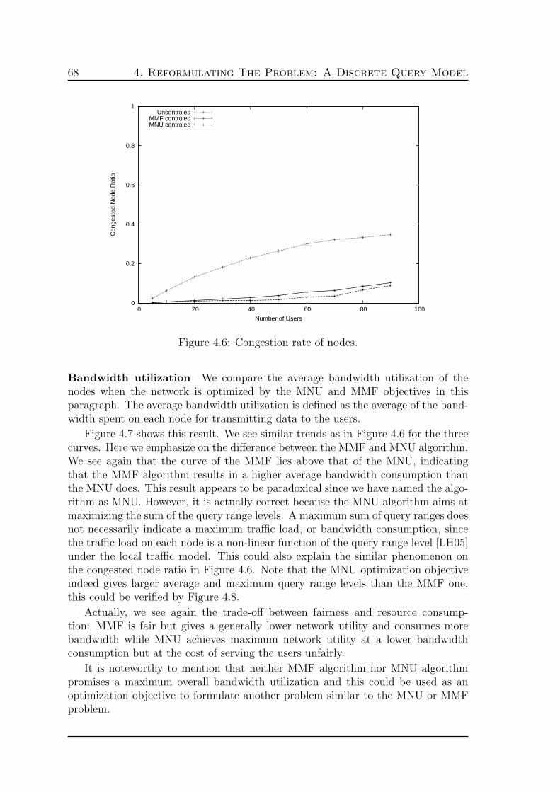
68 4. Reformulating The Problem: A Discrete Query Model

0

0.2

0.4

0.6

0.8

1

0 20 40 60 80 100

Con

gest

ed N

ode

Rat

io

Number of Users

UncontroledMMF controledMNU controled

Figure 4.6: Congestion rate of nodes.

Bandwidth utilization We compare the average bandwidth utilization of thenodes when the network is optimized by the MNU and MMF objectives in thisparagraph. The average bandwidth utilization is defined as the average of the band-width spent on each node for transmitting data to the users.

Figure 4.7 shows this result. We see similar trends as in Figure 4.6 for the threecurves. Here we emphasize on the difference between the MMF and MNU algorithm.We see again that the curve of the MMF lies above that of the MNU, indicatingthat the MMF algorithm results in a higher average bandwidth consumption thanthe MNU does. This result appears to be paradoxical since we have named the algo-rithm as MNU. However, it is actually correct because the MNU algorithm aims atmaximizing the sum of the query range levels. A maximum sum of query ranges doesnot necessarily indicate a maximum traffic load, or bandwidth consumption, sincethe traffic load on each node is a non-linear function of the query range level [LH05]under the local traffic model. This could also explain the similar phenomenon onthe congested node ratio in Figure 4.6. Note that the MNU optimization objectiveindeed gives larger average and maximum query range levels than the MMF one,this could be verified by Figure 4.8.

Actually, we see again the trade-off between fairness and resource consump-tion: MMF is fair but gives a generally lower network utility and consumes morebandwidth while MNU achieves maximum network utility at a lower bandwidthconsumption but at the cost of serving the users unfairly.

It is noteworthy to mention that neither MMF algorithm nor MNU algorithmpromises a maximum overall bandwidth utilization and this could be used as anoptimization objective to formulate another problem similar to the MNU or MMFproblem.

69

0

0.2

0.4

0.6

0.8

1

0 20 40 60 80 100

Ave

rage

Ban

dwid

th U

tiliz

atio

n

Number of Users

UncontroledMMF controledMNU controled

Figure 4.7: Bandwidth utilization of nodes.

Query levels The query range level indicates the utility of a user. We show thedifferences between the networks optimized by the two objectives in this paragraph,by studying the average and the maximum query range of the users. Figure 4.8shows that the MNU optimization objective gives larger average and maximumquery range levels than the MMF does, as already mentioned. More interestingly,we see different trends of the maximum and average query range level as the numberof users increases: the average is monotonically decreasing; the maximum is aroundthe maximum allowed level.

The monotonically decrement of the average query range level is a reasonableeffect of bandwidth sharing among multiple users: as more users are in the network,each user has to shrink its impacted area. In general, the MMF policy requiresnearby users have similar query range levels and a user is able to have a remarkablyhigher query range level only when it is geographically far from the others. As aresult, MMF objective generally gives users smaller chance to achieve maximumallowed level than the MNU objective does. This explains why the former alwaysgives a maximal query range to the users lower than the latter.

Fairness among users More information about how the users are satisfied couldbe provided by demonstrating how the users are distributed in the query rangelevel domain, as shown in Figure 4.9. Three cases with 10, 50 and 90 users areinvestigated and the height of the bar in the figure represents the ratio of the usersthat have the corresponding query range level. Results of the MMF algorithm andthe MNU algorithm are grouped for comparison. We can observe that the MMFalgorithm results in a more concentrate distribution than the MNU algorithm doesunder all the three cases. Actually, the distribution could be used as an indicator of

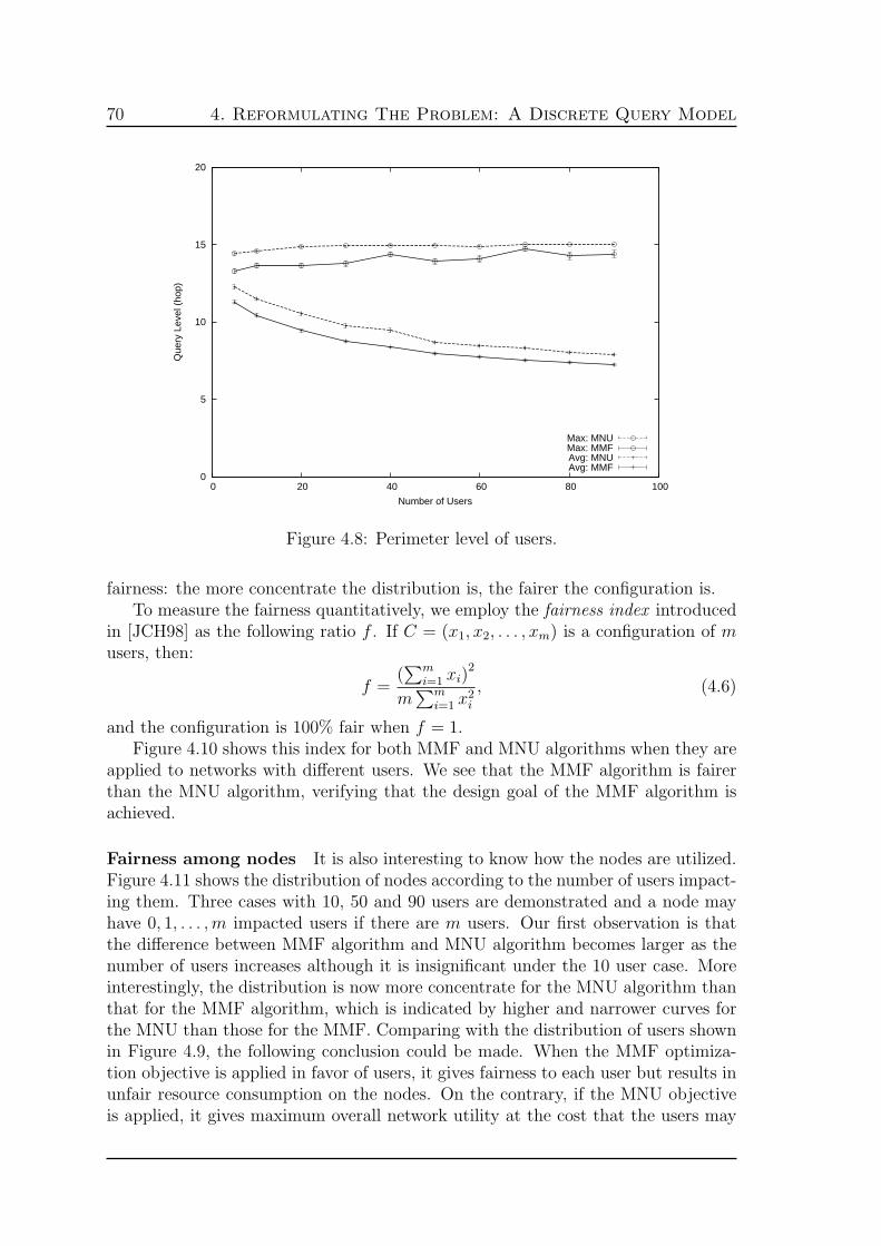
70 4. Reformulating The Problem: A Discrete Query Model

0

5

10

15

20

0 20 40 60 80 100

Que

ry L

evel

(ho

p)

Number of Users

Max: MNUMax: MMFAvg: MNUAvg: MMF

Figure 4.8: Perimeter level of users.

fairness: the more concentrate the distribution is, the fairer the configuration is.To measure the fairness quantitatively, we employ the fairness index introduced

in [JCH98] as the following ratio f . If C = (x1, x2, . . . , xm) is a configuration of musers, then:

f =(∑m

i=1 xi)2

m∑m

i=1 x2i

, (4.6)

and the configuration is 100% fair when f = 1.Figure 4.10 shows this index for both MMF and MNU algorithms when they are

applied to networks with different users. We see that the MMF algorithm is fairerthan the MNU algorithm, verifying that the design goal of the MMF algorithm isachieved.

Fairness among nodes It is also interesting to know how the nodes are utilized.Figure 4.11 shows the distribution of nodes according to the number of users impact-ing them. Three cases with 10, 50 and 90 users are demonstrated and a node mayhave 0, 1, . . . ,m impacted users if there are m users. Our first observation is thatthe difference between MMF algorithm and MNU algorithm becomes larger as thenumber of users increases although it is insignificant under the 10 user case. Moreinterestingly, the distribution is now more concentrate for the MNU algorithm thanthat for the MMF algorithm, which is indicated by higher and narrower curves forthe MNU than those for the MMF. Comparing with the distribution of users shownin Figure 4.9, the following conclusion could be made. When the MMF optimiza-tion objective is applied in favor of users, it gives fairness to each user but results inunfair resource consumption on the nodes. On the contrary, if the MNU objectiveis applied, it gives maximum overall network utility at the cost that the users may

71

0 0.1 0.2 0.3 0.4 0.5

1 2 3 4 5 6 7 8 9 10 11 12 13 14 15

Rat

io

Query Level (hop)

MMF, 10 usersMNU, 10 users

0 0.1 0.2 0.3 0.4 0.5

1 2 3 4 5 6 7 8 9 10 11 12 13 14 15

Rat

io

Query Level (hop)

MMF, 50 usersMNU, 50 users

0 0.1 0.2 0.3 0.4 0.5

1 2 3 4 5 6 7 8 9 10 11 12 13 14 15

Rat

io

Query Level (hop)

MMF, 90 usersMNU, 90 users

Figure 4.9: Distribution of users at each query range level.

0.5

0.6

0.7

0.8

0.9

1

0 20 40 60 80 100

Fai

rnes

s In

dex

Number of Users

MMFMNU

Figure 4.10: Fairness index.

72 4. Reformulating The Problem: A Discrete Query Model

0

0.05

0.1

0.15

0.2

0.25

0.3

0 5 10 15 20 25 30 35 40

Rat

io o

f Sen

sors

Number of Querying Users

MNU 10 usersMMF 10 usersMNU 50 usersMMF 50 usersMNU 90 usersMMF 90 users

Figure 4.11: Node distribution on the number of impacting users.

be served unfairly, but the resulted configuration makes use of the resources on eachnode more evenly. Thus, the MNU may be favorable in particular network designs.For example, in some wireless sensor networks with multiple data collectors, theenergy consumption on each node should be well balanced in order to maximize thenetwork lifetime.

Another interesting observation on the Figure 4.11 is about the ratio of the nodeswith no user impacting them. Over 20% of nodes are not impacted by any user when10 users are in the network while this ratio decreases quickly to about 5% for 50users and 2% for 90 users. This observation may be valuable when the networkcoverage is concerned. Suppose the users are the service providers as the accesspoints in a mesh network while the nodes are the users of such mesh networks. Onedesign concern is how to cover maximum number of the users within a certain regionwith minimum number of randomly deployed access points. However, Figure 4.11shows us that if a certain coverage is required, the number of access points mustachieve a certain threshold. It is impossible to cover the network only by enlargingthe coverage of a few access points.

4.4.4 A dynamic network example

In this final simulation, we try to show how the users cooperate according to Al-gorithm 6 in order to achieve a certain global optimization objective, by a simpleexample. We use the scenario 5 in Table 4.2 and a network topology with 10 users isgenerated for it. The simulation runs for 5000 seconds, however, at the beginning ofthe simulation, only 5 users start working while the rest stay idle until the simula-tion time 1500s. The topologies after 1500s is shown in Figure 4.12(a) and 4.12(b),

73

0

12

3

4

5

6 7

8

9

(a) MMF

0

12

3

4

5

6 7

8

9

(b) MNU

Figure 4.12: Network topology with 10 users and the congested nodes.

for the MMF and MNU cases, respectively. The topologies before 1500s are trivialthus not shown. The congested nodes and the users related with them are depictedwhile other nodes are omitted for clarity.

The users are connected by a link with the congested nodes if their query rangelevels are actually modified by the nodes. These users could be seen as the mostcritical impacting users to the corresponding nodes. Other users around a congestednode may have impacts on it as well, but as their impacts could be so weak thatdecreasing them will not generate a better solution, their query ranges are notmodified by the node. As user 7 to the congested node between user 2 and 6 inFigure 4.12(a). It has impact on the node but its impact level is not modifiedby the node. This phenomenon may be used in developing smarter distributedheuristics. Besides, the number of the congested nodes shown in the figures is trivialas compared to the total population of nodes which is set to 1000 in this example.Together with the limited number of users related with each congested node, onecan expect a limited computation effort has to be spent on the nodes, as well as amodest number of messages have to be generated by those nodes.

Finally, we present Figure 4.13(a) and 4.13(b) to show how the query rangelevels of users evolve, under the MMF and MNU optimization objective, respectively.A common observation is whenever a congestion is detected, the algorithm needssome time to adjust the query range levels between users and then converges atan approximate optimal configuration. Long term evolution of the MMF and theMNU optimized users could be easily distinguished within each clique of users, e.g.{0, 4, 8} and {2, 6}. In the MMF case, query range levels tend to converge to similarvalues while they diverge in the MNU case.

74 4. Reformulating The Problem: A Discrete Query Model

0

2

4

6

8

10

12

14

0 1000 2000 3000 4000 5000

Que

ry L

evel

(ho

p)

Simulation Time (second)

s0s4s8

0

2

4

6

8

10

12

14

0 1000 2000 3000 4000 5000

Que

ry L

evel

(ho

p)

Simulation Time (second)

s2s6s7

(a) MMF

0

2

4

6

8

10

12

14

0 1000 2000 3000 4000 5000

Que

ry L

evel

(ho

p)

Simulation Time (second)

s0s4s8

0

2

4

6

8

10

12

14

0 1000 2000 3000 4000 5000

Que

ry L

evel

(ho

p)

Simulation Time (second)

s2s6s7

(b) MNU

Figure 4.13: Query level evolution of users.

75

4.5 Summary

MMF and MNU optimization objectives have been studied in the chapter. Both ofthem conform with the MMKP formulation which takes the resources constraintson each node into consideration. In consequence, the resulted algorithms are able toprevent the nodes from being congested. Although we consider only bandwidth inthis study, it is possible to generalize to other types of resources e.g. energy, storage,computation power, etc.

The average and maximal query range levels have been inspected and they pro-vide precious indication which may help for dimensioning the wireless sensor net-works. The comparative study on the bandwidth utilization of the two optimizationobjectives has shown that although the MNU maximizes the network utility, theaverage bandwidth consumption on the nodes are not necessarily maximized at thesame time. On the contrary, under all of our simulation scenarios, the bandwidthconsumption of the nodes in a network optimized for MNU is lower than in thoseoptimized for MMF. Furthermore, the distribution of query range levels are moreconcentrate among users under the MMF objective than under the MNU objective,indicating the former gives more fairness to the users. More interestingly, as thenumber of users in the network grows, the distributions tend to concentrate firstinstead of shifting leftwards and this holds for both MNU and MMF objectives al-though it is more obvious for the latter case. This phenomenon implies that thenetwork under local traffic model tries to give more users a medium query rangewhen the number of users grows.

It will be interesting to cope with dynamic networks: transient users and mov-ing nodes are the first challenges on the way to a realistic network. Finally, thedistributed heuristic could be improved by investigating new ways to estimate thetraffic in wireless sensor networks.

76 4. Reformulating The Problem: A Discrete Query Model

77

Chapter 5

Extension To A Practical Context:ZigBee Based WSNs

“ He, who every morning plans the transactions of the day, andfollows that plan, carries a thread that will guide him through alabyrinth of the most busy life. ”

– Victor Hugo

Query allocation problems have been formulated and studied with both continuousand discrete query models for multi-user WSN in previous chapters. In this chapter,we adapt the algorithms for the discrete version of the problem, namely the MMKP-MNU and MMKP-MMF, to a ZigBee cluster tree based wireless sensor network.The rest of the chapter is organized as follows: How to build mobile user WSNsbased on the IEEE 802.15.4 and ZigBee standards is discussed in Section 5.1. Thedistributed algorithm (Algorithm 6) proposed in Section 4.3.2.3 is then adapted tothe ZigBee cluster tree structure, with special considerations on the addressing androuting mechanisms which make the resulted algorithms more efficient with respectto the amount of control messages involved. The adapted algorithms are evaluatedvia simulation in Section 5.3 and we conclude this chapter in Section 5.4.

5.1 The IEEE 802.15.4 and ZigBee Tree

A general description on the IEEE 802.15.4 standard [80206] has been given inSection 2.1.2.2. Specifically designed for low power devices, it allows devices tosleep during the inactive period in a superframe bounded by the beacons. Thesleep mode, which is only available when the network works on a synchronized treestructure, is appealing when energy saving is desired. On the contrary, if the networkworks on a peer-to-peer mode, the lack of synchronization makes the devices keepalive in order to receive from neighbors.

78 5. Extension To A Practical Context: ZigBee Based WSNs

Based on the 802.15.4, the ZigBee specification [zig08] defines addressing, net-work maintenance and routing for unicast, multicast or broadcast packets at networklayer. We have discussed the basic functionalities provided by the ZigBee specifi-cation in Section 2.1.2.3. Especially, the cluster tree routing does not employ anyrouting discover packets thus it is more appealing for energy constrained networkssuch as WSNs.

Building multi-user WSN based on ZigBee network is straightforward. However,some choices have to be made to fit the special requirements of multi-user WSN.In a WSN, the routers are usually at the same time the sensor nodes, thus aresupposed to be battery powered. This energy issue advocates for the tree operationmode proposed by ZigBee. Network maintenance when multiple users join and leavecan be easily implemented in the ZigBee infrastructure with full conformance. Forexample, a user may use the ZigBee join procedure to connect to the network andfollow the leave procedure when it moves outside the parent and later reconnect toother nodes with the rejoin procedure.

Furthermore, a user may act as either end devices or routers in the ZigBeenetwork. If mobility is considered, the movement of the user router may result inreconstruction of the subtree rooted at itself. In this study, we confine the users toact only as end devices, thus the backbone of the cluster tree can be kept intacteven when the users move.

A user initiates a query in order to collect data from the sensors. Motivated bythe application scenarios introduced previously, we suppose the query is sent to allsensor nodes within a certain number of hops to the user then all such sensors willsend data back to the user at the required rate repeatedly until modified by anotherquery. The queries are sent via hop-bounded flooding on the tree and data is sentback via unicast cluster tree routing, both supported by the ZigBee specification.Specifically, the former can be done by checking the query message header for theradius field on the router, and rebroadcasting the message if radius is positive, toits on-tree neighbors except the one from which the message is received. For thelatter, we assume sensors send a copy of the same data to each querying user ratherthan using multicast. Figure 5.1 illustrates an example multi-user WSN with twousers and a query at radius of 3 hops.

ZigBee Coordinator

UsersZigBee RouterZigBee End DevicesQuery

Data

Figure 5.1: Multi-user WSN based on ZigBee tree structure.

79

Lm− 1

d

(a)

Representative

EQ1

(h, hs) = (d, 0)

(d− 1, 1)

(d− 2, 2)

(1, d− 1)

(0, d)

(1, d + 1)

(d, 2)

(Lm− 1, Lm− d + 1)

(Lm− 1, Lm− d + 3)

(Lm− 1, Lm + d− 3)

(Lm− 1, Lm + d− 1)Rm− 1

(b)

Figure 5.2: Two views of a ZigBee routing tree. (a) Tree T , rooted at the coordina-tor, (b) Tree Ts, rooted at the user, labels assigned to devices.

5.2 Algorithms Adapted to the ZigBee Network

The distributed algorithms (the Algorithm 6) for both MMKP-MNU and MMKP-MMF have been proposed in Chapter 4. The basic idea is to solve a MCKP ateach congested sensor and then feed the results back to the related querying users.The adaptation of these algorithms to the ZigBee tree network consists of only anew traffic estimation mechanism that exploits the special property offered by thecluster tree addressing and routing mechanisms.

5.2.1 Traffic estimation with the ZigBee tree

When the sensor notices a congestion is about to happen, the traffic estimation isemployed to calculate optimal query allocation for the users querying it. Trafficcould be estimated through various ways and here we propose a local estimationprofiting the ZigBee address structure. The aim is to give an estimation about theincrement of the number of devices involved if the query range becomes one hoplarger. Intuitively, the additional traffic load comes from those devices.

Consider the ZigBee network which is a tree T rooted at the ZigBee coordinator,as shown in Figure 5.2(a). For the querying user s, the whole network could beseen as a tree Ts rooted at itself. Thus for a router, the additional traffic passingthrough comes from the to-be-covered devices that are his descendent on Ts. Alogical structure of Ts is illustrated in Figure 5.2(b). We assign a label (h, hs) toeach device in the network, where h and hs denote the depth of the device on T andTs, respectively. Note that every device knows h on joining the network. On theother hand, for a given device, hs is actually its hop distance to s, which could beobtained simply by inspecting the received query message originated from s.

Then we divide the routers (including the ZigBee Coordinator) into several equiv-alent classes according to their labels. Each equivalent class consists of a sub-treerooted at a router on the path from the user to the coordinator. Obviously, there

80 5. Extension To A Practical Context: ZigBee Based WSNs

∆nR(i, hs, k) =

{Rmk−hs+1, if hs − 1 ≤ k ≤ Lm− d+ 2i− 20, otherwise (5.4)

∆rR(1, 1, k) =

Rm∆nR(1, 2, k) + ∆r

R(2, 2, k), if 0 < k ≤ Lm+ d− 21, if k = 00, otherwise

(5.5)

∆rR(i, i, k) =

(Rm− 1)∆nR(i, i+ 1, k) + ∆r

R(i+ 1, i+ 1, k), if i− 1 < k ≤ Lm− d+ 2i− 21, if k = i− 10, otherwise

(5.6)

are d such equivalent classes. Let EQi be the ith equivalent class and we have:

EQi = {r|h− hs = d− 2i}, (1 ≤ i ≤ d). (5.1)

The router with hs = i is referred to as the representative router of the equivalentclass, noted as ri. For example the routers with label (d − 1, 1), (d, 2), . . . , (Lm −1, Lm− d+ 1) belongs to EQ1 and (d− 1, 1) is the representative router. As shownin Figure 5.2(b), the routers of EQ1 are grouped into a shadowed area.

Now consider a router in r ∈ EQi with label (h, hs), let ∆R(i, hs, k) be thenumber of additional routers and ∆E(i, hs, k) the number of end devices that willbe handled by r when the query range increases from k to k + 1. If every devicesend data at constant rate b, the additional traffic load ∆T (i, hs, k) should be:

∆T (i, hs, k) = b (∆R(i, hs, k) + ∆E(i, hs, k)) . (5.2)

Now we derive ∆R(i, hs, k), then ∆E(i, hs, k) could be obtained as the following:

∆E(i, hs, k) = ∆R(i, hs − 1, k − 1)(Cm−Rm). (5.3)

In order to calculate ∆R(i, hs, k), we further separate the non-representativerouters and the representative routers and denote the corresponding ∆R function as∆nR and ∆r

R.Then we have (5.4) for a non-representative router, where 1 ≤ i ≤ d and i+ 1 ≤

hs ≤ Lm − d + 2i − 1. For a representative router, which implies hs = i, we have(5.5) and (5.6) for i = 1 and i > 1 cases, respectively.

One remark about the estimation proposed above is that it obtains an upperbound of the additional traffic and this upper bound is reached only when thenetwork address is fully used by the devices. However, this condition is hardly metin practice, thus the estimation usually deviates from reality. As a countermeasure,we propose to apply a scaling parameter to the estimated traffic to account foraddress utilization. For example, routers may obtain such a scaling parameter fromthe number of addresses allocated to its children and its available address block.

The new traffic estimation method could be applied directly by each node k tocalculate M(k). As a result, Algorithm 5 and 6 could be used with minor modifica-tions.

81

Table 5.1: Evaluation metrics.Parameter Definition

Tapp = Query data receive bit rate at users

γ = Tapp

Query data sent bit rate

Omac = MAC layer control message sent bit rateTapp

Oapp = Application layer control message sent bit rateTapp

I = sum of query level of usersnumber of users ,

at a certain simulation time.

I∗ same as I, obtained by an exact algorithm.

f = (Pmi=1 xi)2

mPm

i=1 x2i

,m: number of queries,xi: query radius of user i.

5.3 Performance Evaluation

In this section, we evaluate the proposed algorithms by comprehensive simulations.We implemented the proposed algorithms and the basic functionalities of the Zig-Bee network layer on top of IEEE 802.15.4 implementation [ZL] in the ns2 simula-tor [ns2].

5.3.1 Evaluation metrics

We will evaluate the following metrics: query data throughput (Tapp), query dataarrival ratio (γ), MAC layer control message overhead (Omac), application layercontrol message overhead (Oapp), query radius and fairness index (f). The definitionsare presented in Table 5.1.

5.3.2 Simulation setup

Table 5.2 summarizes the simulation parameters. We evaluate our algorithm in twokinds of networks: a grid network and a network with uniformly deployed nodes.The size of the network are chosen to cover a small network and a large network,with 50 nodes in 100 by 100 meters square, 100 nodes in 140 by 140 meters square,respectively.

We also select two representative values of the queried data rate: for a light loadnetwork, each node on query send data at 100bps, which corresponds to sending a28 bytes of data every 2.24 seconds; for a heavy load network, the query data rateis 800bps or 28 bytes of data every 0.42 seconds. We use this fixed data message

82 5. Extension To A Practical Context: ZigBee Based WSNs

Table 5.2: Simulation parameters.

Topology 1: 50 nodes at 100m×100m, 2 users2: 100 nodes at 140m×140m, 4 users

Node distribution Grid with 14m interval / UniformMAC layer IEEE 802.15.4, BO = SO = 6,

Lm = 10, Cm = 3, Rm = 3MWK layer ZigBee cluster tree routing

Wireless Tx/Rx 15m transmission range,two ray ground,omniscient antenna model

Bandwidth 250kbps at 2.4GHz bandQuery data rate Light load: 100bps, High load: 800bpsSimulation time Query start: 70s,

query stop 300s,simulation stop: 350s

length in our simulation, following the default data length defined in TinyOS [Lev]for CC2420 transceiver.

We start the nodes at the beginning of the simulation with random jitters andthe nodes will continue trying to join the network until it succeeds, except node 0who will create the ZigBee network. The network formation takes about 60 secondsthus we start the queries at 70 seconds. To let the simulation shut down gracefully,we stop all the queries 50 seconds before the simulation stops.

5.3.3 Query data arrival ratio

Let us consider how well multiple queries are handled in the network controlled bythe distributed algorithms, by inspecting the query data arrival ratio. As compari-son, we also run the network without control algorithm. The results are presented inFigure 5.3. We see that the uncontrolled network delivers the queried data at a rela-tively low ratio than the controlled network. The arrival ratio dropped very quicklyafter the queries are diffused in the network. For a heavy load network (b = 800),less of congestion control is generally detrimental: the arrival ratio could be as low as0.3 for large grid network and around 0.4 for both large and small uniform networks.This is unfavorable. On the contrary, a query radius control with either MNU orMMF objective could prevent the network from congestion, thus resulted in higherdata arrival ratio. In a small network with light query load, the query control didnot gave noticeable improvement on the arrival ratio compared with uncontrolledcase. Actually, there is almost no congestion in the network under this case and theeffect of the query control is not obvious.

5.3.4 Query data throughput

The aggregated throughput of the query data provides more information aboutthe performance of the network. Figure 5.4 presents this result. Intuitively, the

83

0

0.2

0.4

0.6

0.8

1

γ small network, light load

MMFMNU

uncontrolled

0

0.2

0.4

0.6

0.8

1

100 150 200 250

γ

Time (second)

small network, heavy load

large network, light load

100 150 200 250 300

Time (second)

large network, heavy load

(a) Grid

0

0.2

0.4

0.6

0.8

1

γ small network, light load

MMFMNU

uncontrolled

0

0.2

0.4

0.6

0.8

1

100 150 200 250

γ

Time (second)

small network, heavy load

large network, light load

100 150 200 250 300

Time (second)

large network, heavy load

(b) Uniform

Figure 5.3: Application data arrival ratio.

84 5. Extension To A Practical Context: ZigBee Based WSNs

control algorithm will confine the query radii from going too large, so will limit thetotal number of sensor nodes under query. This may result in a lower throughput.However, if the network is congested, the throughput may be even lower than anuncongested network with smaller queries. This phenomenon can be observed in thelarge grid network under heavy load case (bottom right plot of Figure 5.4(a)).

5.3.5 Control message overhead

We are interested in how much it costs to achieve query control in the proposed queryscheme and the distributed algorithm. We shall investigate this issue by inspectingboth the MAC layer and the application layer control overhead. Note that thenetwork layer does not impose any overhead after the network formation thanksfor the cluster tree routing. Even during the network formation period, the networklayer requires only several message exchange for one device to join the network. Thisoverhead is negligible comparing with those in the normal operation period.

In MAC layer, the overhead comes from the beacon message, the acknowledg-ment and the ARP packets, while in application layer, it comes from the querymessage and the adjust-level message as described in Algorithm 6. Figure 5.5 showsthe overhead for both layers in different network settings. The values could be in-terpreted as how many bits of control message is needed for successfully deliveringone bit of query data. At MAC layer, we observe a sharp decrement of the overheadwhen the query load goes high, for both grid and uniform networks.

In application layer, the uncontrolled networks always have negligible overhead,independent to the network size, the node distribution or the query load. In contrast,the control overhead goes abruptly for networks with either MNU or MMF whenthe query load is light. However, under heavy load case, the overhead could be keptalmost constant when the network size increases. Combined with Figure 5.3 and 5.4previously discussed, the query control mechanisms are more efficient under heavyload case than under light load case.

5.3.6 Query range and fairness index

The average query range of the 4 users in the large network, obtained by both thedistributed algorithms and an external problem solver is plotted in Figure 5.6. Theexternal problem solver obtains an optimal solution for both MNU and MMF withthe traffic information traced from the uncontrolled network. We see that for MMFcase, the approximation is quite near to the optimal. While for MNU in a light loadnetwork, the optimal is further above what the distributed algorithm can achieve.Furthermore, we can observe that the difference between optimal and simulationvalues is larger under light load cases than heavy load cases, under MNU cases thanMMF cases. The explanation is as follows. Normally, the ‘select the minimum’strategy used in Algorithm 6 gives a user more chances to follow a smaller queryrange, especially when the users have more possibility to choose different queryrange values. This is actually a cavity of the ‘select the minimum’ strategy. Byinspecting more carefully on the local solutions found on the congested sensors, we

85

0

1

2

3

Tap

p (1

0Kbp

s)

small network, light load

MMFMNU

uncontrolled

0

1

2

3

100 150 200 250

Tap

p (1

0Kbp

s)

Time (second)

small network, heavy load

large network, light load

100 150 200 250 300

Time (second)

large network, heavy load

(a) Grid

0

1

2

3

Tap

p (1

0Kbp

s)

small network, light load

MMFMNU

uncontrolled

0

1

2

3

100 150 200 250

Tap

p (1

0Kbp

s)

Time (second)

small network, heavy load

large network, light load

100 150 200 250 300

Time (second)

large network, heavy load

(b) Uniform

Figure 5.4: Aggregated application data throughput.

86 5. Extension To A Practical Context: ZigBee Based WSNs

0

1

2

3

4

5

6

Οm

ac

light loadheavy load

0

1

2

3

4

5

uncontrolled MMF MNU

Οap

p small network

uncontrolled MMF MNU

large network

(a) Grid

0

1

2

3

4

5

6

Οm

ac

light loadheavy load

0

1

2

3

4

5

Uncontrolled MMF MNU

Οap

p small network

Uncontrolled MMF MNU

large network

(b) Uniform

Figure 5.5: Protocol overhead.

87

0

4

8

12

Que

ry L

evel

(ho

p)

MNU, light load

Ι∗ = 8.5

0

4

8

12

100 150 200 250

Que

ry L

evel

(ho

p)

Time (second)

MMF, light load

Ι∗ = 8.0algorithm Ι

fairness indexoptimal (Ι∗ )

0.8

0.85

0.9

0.95

1

Fairness Index

MNU, heavy load

Ι∗ = 4.5

100 150 200 250 0.8

0.85

0.9

0.95

1

Fairness Index

Time (second)

MMF, heavy load

Ι∗ = 4.5

(a) Grid

0

4

8

12

Que

ry L

evel

(ho

p)

MNU, light load

Ι∗ = 8.0

0

4

8

12

100 150 200 250

Que

ry L

evel

(ho

p)

Time (second)

MMF, light load

Ι∗ = 7.5

algorithm (Ι)fairness index

optimal (Ι∗ )

0.8

0.85

0.9

0.95

1

Fairness Index

MNU, heavy load

Ι∗ = 4.75

100 150 200 250 0.8

0.85

0.9

0.95

1

Fairness Index

Time (second)

MMF, heavy load

Ι∗ = 3.25

(b) Uniform

Figure 5.6: Query radius evolution of users.

88 5. Extension To A Practical Context: ZigBee Based WSNs

found that the obtained query ranges are quite dispersed sometimes. However theaverage is near to the optimal value, e.g. at certain time in a simulation run, thequery range calculated on two sensors could be (6, 5, 10) and (5, 10, 6) for 3 users,both resulting an average of 7. However, this diversity is eliminated at the users byalways choosing the minimal, e.g. users have to choose 5, 5, 6 as their final results.This problem becomes less obvious when the local solution gives users similar queryranges. Finally, one may wonder why the approximation over-performs the optimalin the MMF heavy load case. This is actually due to the linear increment usedto further explore the potential larger feasible query range. If the local solutionsuggested by the congested sensors is already very near the optimal, the explorationprocedure may generate transient congestion state in the network. We leave theseproblems for future works.

Finally, fairness index of the 4 users in the network is plotted for MNU and MMF.Since MMF generally gives similar query range to the users, its f values are higherthan those of MNU under the same network situation. This could be examined bycomparing the f plots in Figure 5.6 vertically, justifying the optimization objectiveof MMKP-MMF.

5.4 Summary

Mobile user network structure hence the resulted direct interaction between usersand sensors can be implemented on IEEE 802.15.4 and ZigBee standards in thischapter. Algorithms for MMF and MNU, proposed in Chapter 4, have been adaptedto the ZigBee cluster tree in this chapter. By exploiting the ZigBee cluster treestructure, the computation was done fully locally. Simulation results have shownthat: firstly, the new algorithms do well in congestion control with little overheadand they are especially efficient in large networks with heavy queries; secondly,MMKP-MMF algorithm works better than MMKP-MNU in approximating theiroptimal solutions on the ZigBee cluster tree.

89

Chapter 6

The Problem Behind: EmpiricalStudy On The Hard MMKPInstances

“ Nothing in life is to be feared. It is only to be understood. ”– Marie Curie

We have formulated the discrete version of the query allocation problem for themobile-user wireless sensor networks with the multidimensional multiple choice knap-sack problem in Chapter 4. An overview on the KP and MMKP problems has beengiven in Section 2.3. Exact and heuristic algorithms for MMKP proposed in previousworks have been discussed in Section 2.3.1 and Section 2.3.2, respectively.

In this chapter, we focus on this hard combinatorial problem itself. We developour idea in this chapter with the following sections: A brief introduction is givenin Section 6.1, mainly to motivate the empirical study presented in this chapter.Then we give a brief survey of existing benchmarking methods in Section 6.2. Thenin Section 6.3, we propose new methods to generate MMKP benchmark instances.Section 6.4 is dedicated to evaluating the difficulty of these instances using the exist-ing exact algorithm and solvers. Finally, we draw conclusion and propose importantfuture works in Section 6.5.

6.1 Introduction

Multidimensional Multiple choice Knapsack Problem (MMKP) is one of the mostcomplex members of the Knapsack Problem (KP) family. It could be stated asfollows: We are given m classes with each class i containing ni items. The jth itemof class i has profit pij. Each item has l dimensions of weight, and the weight atdimension k is denoted as wijk. The knapsack has capacity ck on each dimension k.The goal is to select one item in each class to maximize the sum of their profits and

90 6. Hard MMKP Instances

to keep the total weight on each dimension no more than the corresponding capacity.Formally, MMKP could be expressed with an integer programming model:

(MMKP) maximizem∑i=1

ni∑j=1

pijxij (6.1)

subject tom∑i=1

ni∑j=1

wijkxij ≤ ck, k = 1, . . . , l (6.2)

ni∑j=1

xij = 1, i = 1, . . . ,m (6.3)

xij ∈ {0, 1}, i = 1, . . . ,m, j = 1, . . . , ni (6.4)

where the binary variable xij indicates the jth item of class i is selected or not.For clarity, we assume all classes have the same number of items in this study, i.e.n1 = · · · = nm = n.

MMKP has many applications. It has been used to model the Quality of Service(QoS) management problem in computer networks [LLRS99] and the admissioncontrol problem in the adaptive multimedia systems [SIH05, Kha98, KLMA02].Various other resource allocation problems can also be mapped directly to MMKP,please refer to [KPP04, PHD05] and the references wherein.

Most academic efforts related with MMKP have been put on finding heuristicalgorithms due to the NP-hard nature of the problem [KLMA02, MJS97, HMS06,ARK+06]. However, computing exact MMKP solutions can also be of interest whenthe computation time constraint is not critical, e.g. exact solution is the mostvaluable benchmark for the heuristic algorithms. More important, when the exactalgorithms can solve most problem instances quickly and only fall into exponentialtime in rare cases, they can be applied to some practical problems. Thus, for anyexact algorithm, it is important to know how often it falls into the trap.

Great efforts have been taken in analyzing the structure of many KP family mem-bers, e.g. simple KP, Bounded KP (BKP), Multiple KP (MKP), Multiple ChoiceKP (MCKP), Multidimensional KP (MDKP) etc. Comprehensive discussions onthese problems could be found in [HMS75, KPP04]. It has been demonstrated thatall of them are highly structured. Exploiting their special structural properties usu-ally leads to efficient algorithms that are able to solve certain category of probleminstances in reasonable time, although the problems are NP-hard. Moreover, it ap-pears that some instances are particularly hard to solve not because of the size ofthe problem (number of input variables or the magnitude of the variable values),but because of the special combination of variable values, i.e. even a small probleminstance can require a long time to solve. Generally, the relationship between theprofits and weights of the items plays a very important role in the solution time ofcertain problem instances. Besides, a very important observation has been made onsimple KP that the relationship between the capacity and the weight also has greatimpact on the hardness of the instances [Pis99].

91

In contrast, little work has been done on MMKP in analyzing its structure. Tothe best of our knowledge, besides many proposed algorithms, the only theoreticalanalysis is presented in [DW98]. The authors show that the proportion of thedominated variables can be estimated as a probability function of the number ofdimensions and the number of items in each class. The results could be used toreduce the problem size during the pre-process stage. However, it is still unclear howthe parameters such as profit, weight and capacity interact in making the problemdifficult. Furthermore, almost all MMKP algorithms proposed in the literature areevaluated against very limited problem instances which may belong to special easycases.

In this chapter, we study the relationship between various parameters of theMMKP such as profit, weight and capacity in order to identify the key factors thatmake a hard instance. Furthermore, uncorrelated, weakly correlated and stronglycorrelated cases for items within each class, between classes and across multiple di-mensions are investigated. To the best of our knowledge, no such work has beenreported in the current literature. A systematic method to generate comprehen-sive MMKP test instances is proposed. Several groups of instances generated withthe proposed methods are evaluated with the exact algorithm and solvers. The ex-periments show that many instances are several orders of magnitude harder thantraditionally used ones in terms of the computing time. These hard MMKP instancesusually have medium knapsack capacity and high correlation between weights andprofits. The experiments also suggest that instances with similar set of profits acrossclasses and with strong correlations between weights and profits are hard to solve.

Two exact algorithms are currently available for solving the MMKP, namely theBBLP algorithm [Kha98, KLMA02] and the EMKP algorithm [Sbi07], which havebeen discussed in Section 2.3.1. Besides, two integer programming solvers, ILOGCPLEX [cpl] and GLPK [glp] exist. However, we have identified some fundamentalproblems of the EMKP algorithm [Sbi07]. First of all, the EMKP algorithm employsbasically a sequential search strategy, i.e. the development of a certain node dependson its previous brother nodes. This prevents pruning the infeasible nodes effectivelyas some feasible nodes may have to be developed from them. Secondly, the EMKPalgorithm selects the best node to develop at each round, but the paper does notstate how the selection is made. A common way is to select the node with thehighest upper bound. However, for the infeasible nodes which are kept in the searchtree, there is no natural way to calculate an upper bound. Finally, the sequentialsearch strategy implicitly requires generating the brother node for every node whohas a brother. This is true even for the unpromising nodes whose upper boundis below the lower bound. However, EMKP tries to reduce the search space bypruning these unpromising nodes (line 17 of the algorithm in [Sbi07]). This willbreak the searching process and the algorithm will not be able to find the optimalsolution which have to be reached through the pruned node. Even worse, the betterthe quality of the lower bound is (approaching the optimal from below), the moreoften the improper prune may happen. As a result, we will consider only the BBLPalgorithm and two generic MIP solvers GLPK and CPLEX in this study.

92 6. Hard MMKP Instances

6.2 Existing Methods to Generate Benchmark In-

stances

It is very important to test the algorithms with problem instances in order to knowtheir performance in practice. When algorithms are tackling a particular problem,ideal instances for performance evaluation are those from traces of the real world.However, as MMKPs usually originate from a diverse applicative background, typi-cal instances from a certain domain may hardly be reasonable for another. Moreover,there is no systematic report on real world MMKP problem instances in the litera-ture. In contrast, test instances can be generated to cover a much wider range of in-stance types. As a result, generated instances play an important role in benchmark-ing the algorithms and have been used in most KP and MMKP related researches.In the following, we first describe how the KP instances are usually generated, thenwe give a brief review on the current method to generate the MMKP instances. Thelatter is basically a straightforward extension of the former.

6.2.1 Generating KP instances

In order to generate a KP instance with certain number of items, the idea is to firstassign values to both profit and weight of each item, then to set the capacity of theknapsack. Several groups of instances have been identified for KP considering thecorrelation between the profits and weights [Pis05].

- uncorrelated instances. For this category, the profit of an item is independentto its weight. A commonly used method is to select profits (pj) and weights(wj) randomly in a certain interval, e.g. [1, R]. These instances are generallyeasy to solve.

- weakly correlated instances. In weakly correlated instances, the profit of anitem is related with its weight, e.g. to select wj randomly in [1, R] and pj in[wj −R/10, wj +R/10] while ensuring pj ≥ 1.

- strongly correlated instances. For these instances, the profit of an item is alinear function of its weight plus a certain shift, e.g. to select wj randomly in[1, R], but let pj = wj + R/10. This category of KP instances are generallyhard to solve.

- sub-set sum instances. For this category of instances, the profit of an item isa linear function of its weight. As a result, only weight need to be consideredwhen packing the knapsack.

Instances with other types of correlation can be defined similarly [Pis05].

Finally, the capacity of the knapsack is set to a certain percentage of the sumweight. However, this has been shown to be inadequate as it generates the easiestKP instances under certain situations [Pis99]. Thus the idea consists of generating

93

a series of S test instances with the capacity c of the hth instance selected as:

c =h

S + 1

n∑j=1

wj. (6.5)

6.2.2 Generating MMKP instances

To generate an MMKP instance with a given number of classes, a given number ofitems in each class and a given number of dimensions, the problem is to assign aprofit value to each item, a weight value to each item at each dimension, and finally,a capacity value to each dimension of the knapsack. This can be done in variousways.

In [KLMA02], weights of items are uniformly selected in the interval [0, R] in-different to the dimensions or which class the item belongs to, where R denotesthe maximum resource consumption by an item. Let P denote the maximum costof unit resource, then the value R × P could be considered as the maximum cost(weight) of an item. Then uncorrelated instances are generated with profits assignedaccording to the item index in the class:

pij = U(

0, l × R

2× P

2

)× j + 1

ni. (6.6)

For correlated instances, the profit is a linear function of the sum weight:

pij =l∑

k=1

Pkwijk × U(

0, l × 3× R

10× P

10

), (6.7)

where Pk = U(0, P ) is a uniform random number between 0 and P .Finally, the capacity of dimension k is set to half of the maximum possible

resource consumption:

ck =1

2×m×R. (6.8)

The same set of instances have been used in [Kha98, PHD05, ARK+06, CA06].Instances generated with the same principle have been used in [HMS04, HMS06,CH08]. These instances are available at the OR Benchmark Library [OR-].

In [Sbi07], test instances are generated as follows: pij and wij are randomlyselected in intervals [0, 150] and [0, 50], respectively. Capacities are set as:

ck =1

2

m∑i=1

(wminik + wmax

ik

), (6.9)

where

wminik = min

1≤j≤n{wijk}, (6.10)

wmaxik = max

1≤j≤n{wijk}. (6.11)

94 6. Hard MMKP Instances

In [AHHS05], domain related values are considered in the test instances. Thenumber of classes, items in each class and dimensions are set according to a typicalVideo on Demand (VoD) system. The variable values are also set with respect tothe typical values of a VoD system. For example, the weight of each item is set tothe typical resource consumption of a session. The value is then scaled by a randomnumber chosen from the interval [0.75, 1.25] to mimic system dynamics. Similarly,the capacities are set to typical available resources scaled by a random value chosenfrom the interval [0.95, 1.05].

Although these instances have been widely used in the literature, our computa-tional results show that they are insufficient in demonstrating the performance ofthe algorithms. Table 6.1 presents the time used to solve the first few instances inthe OR benchmark library with CPLEX, GLPK and the BBLP algorithm. Here weemphasize on the relative solution time across the instances. Notably, instances I3and I4 take much more time than I5 and I6, despite they are smaller than the latter.This actually implies that not only the size of the instance, but also the structureplay very important role in the solution time.

Table 6.1: Solution time (second) of OR benchmark library instances I1 to I6.

Inst m n l CPLEX GLPK BBLPI1 5 5 5 0.005 0.028 0.016I2 10 5 5 0.006 0.029 0.033I3 15 10 10 1.983 16.036 67.260I4 20 10 10 31.045 1383.251 1532.059I5 25 10 10 0.018 0.046 0.660I6 30 10 10 0.204 0.190 2.369

6.3 New Methods to Generate MMKP Problem

Instances

Experiences from KP suggest that the correlation between profits and weights iscritical to the hardness of an instance. Extending this idea to MMKP, we need tohandle the correlation between the profits and multiple dimensions of weights. Onedirect way is to select the profit for each item then select the weights according tothe profits. Given the number of classes (m), the number of items in each class (n,assuming all classes have the same number of items), and the number of dimensions(l), the MMKP is denoted as P (m,n, l). We will also refer to a mapping from aclass of n items to n values informally as a generating function.

6.3.1 Generating the Profits

In order to select the profits for items in each class i, we first bound the profitswith two parameters pmin

i and pmaxi and select profit values within the interval. This

could be done in various ways and here we define some generating functions for theprofits.

95

Uniform Generating Function Uniform random profits are natural in manyreal world problems and are widely used in the literature. In uniform generatingfunction, we draw profit uniformly and randomly within the interval. We denotethe uniform generating function as:

pij = U(pmini , pmax

i

). (6.12)

Linear Generating Function Items with linear profits are less studied in theliterature. However, this kind of profit value assignment is actually quite common.For example in the QoS adaption problem [AHHS05], the QoS levels are usuallymapped to the profit of items and their values are often consecutive integers. Alsoin the multi-hop query allocation problem [HLS09], the query range is mapped to theprofit and is measured in hop numbers which take also consecutive integer values.

In the linear generating function, we assign pij with a linear function of the itemindex j, i.e.

pij =j − 1

ni − 1

(pmaxi − pmin

i

)+ pmin

i . (6.13)

For clarity, we use a short hand notation for this linear generating function as follows:

pij = L(pmini , pmax

i

). (6.14)

Applying the Profit Generating Functions The generating functions shouldbe applied on each single class to generate the profits. Obviously, one can apply thesame function to all classes or change the functions for each class. For the uniformgenerating function, even when it is applied to all classes with the same parameters,the random nature of the function will give different values for profits in differentclasses. On the contrary, when the linear generating function is applied to all classeswith the same parameters, all classes will have the same profit vector for their items.Therefore, besides applying the same generating function to all classes, we furtherpropose two ways to use the generating functions. The first one is to reproduce therandom profit vector generated by a uniform generating function on all classes. Thisis typically the case when several users (classes) can access the same set of objects(items) with varying quality of service (profits) but the cost of accessing them differs(weights). We explicitly denote the profits generated via this way as:

pij = R(U(pmin

1 , pmax1

)). (6.15)

Here, R signifies Reproducing the first generated profit vector for other classes.The second way to apply the generating functions is to take into account the classindex i when deciding the interval from which the values are taken for each class,e.g. U(10(i − 1), 10i) or L(10(i − 1), 10i). When the uniform generating functionis applied this way, the resulted profits in each class is still randomly selected butprofits of different classes are dispersed into different intervals. While the lineargenerating function is applied, the profits are linearly assigned in different intervals.We denote this special application of generating functions as:

pij = C(F ), (6.16)

96 6. Hard MMKP Instances

where F is a generating function with different parameters for different classes andC signifies that the generating function is Class-dependent.

6.3.2 Generating the Weights

To generate the weights, we can apply a certain correlation on the generating func-tion for each dimension. In particular, we define the following generating functions.

Uncorrelated Generating Function In uncorrelated generating function, wesimply assign weights with values uniformly and randomly selected within a certaininterval:

wijk = U(wminik , wmax

ik

). (6.17)

Weakly Correlated Generating Function This generating function is moti-vated by previous results on KP instances [Pis05]. The motivation is to slightlyassociate profits to weights, but still with a degree of freedom for each dimension.In our proposal, weights are assigned according to:

wijk = U(

max

(0, pij −

pmaxi

δ

), pij +

pmaxi

δ

). (6.18)

We will use the following shorthand notation:

wijk =W(δ). (6.19)

Strongly Correlated Generating Function Strongly correlated generating func-tion is also motivated by previous results where the correlation between profits andweights is strong:

wijk = pij +pmaxi

δ. (6.20)

We use the following short hand notation for this function:

wijk = S(δ). (6.21)

Inversed Strongly Correlated Generating Function For inversed stronglycorrelated generating function, weights are assigned according to:

wijk = pmaxi − pij

δ, (6.22)

and will be referred to as:wijk = I(δ). (6.23)

Note that the inversed strongly correlated generating function is not interestingto be used alone. Interesting cases occur when both strongly correlation and in-versed strongly correlation coexist on different weight dimensions. Intuitively, theseinstances are hard to solve because careful trade-off between weights across dimen-sions has to be made. Although we are not aware of any realistic MMKP problemsof this type, they are still interesting from a theoretical point of view.

97

Applying the Weight Generating Functions Similar to the profit generatingfunctions, one could apply the same generating function with the same parameter toall dimensions. But it is also possible to apply the same function with different pa-rameters or even different generating functions for dimensions. In addition to simplyapplying the same generating function with the same parameters on all dimensions,here we propose two ways to apply the weight generating functions. The first one isto include the dimension index k as a parameter of the generating function so thatthe weight for a dimension k can be chosen in a range that depends on k for theuniform generating function, or the parameter δ can be a function of k for weakly,strongly and inversed strongly correlated generating functions. It is convenient touse a shorthand as follows:

wijk = D(F ), (6.24)

where F can be, for example, U(1, 10k) for the uniform generating function, orW(k+5) and S(k+5) for weakly correlated and strongly correlated generating func-tions, respectively. Here, D signifies that the generating functions are Dimension-dependent. We could also apply different generating functions to different dimen-sions, for example, we will generate instances with the inversed strongly correlatedgenerating functions on some dimensions and strongly correlated generating functionon others. Under this case, we denote:

wijk = D(F1F2 . . . ), (6.25)

where F1, F2, . . . are the generating functions in used.

6.3.3 Generating the Knapsack Capacities

Finally, knapsack capacities are generated by extending (6.5) to multiple classes andmultiple dimensions. We generate a series of the S instances and the capacity ofthe kth dimension of the hth generated instance (h = 1, 2, . . . , S), denoted as chk, isdispersed from the minimum possible weight to the maximum possible weight:

chk =h

S + 1

(m∑i=1

wmaxik −

m∑i=1

wminik

)+

m∑i=1

wminik . (6.26)

The parameter h will also be referred to as the capacity level of the instance in theseries. Note that all the S instances do not need to have the same items (profitand weight assignment). However, in order to investigate the impact of the capacitylevel on the solution time, we let all S instances in the same series have the sameprofit and weight values. As a result, instances in a series differ from each otheronly by their capacities.

6.3.4 Summary of Instance Notations

We denote G-x-y a group of instances. The parameter x indicates the gener-ating function that is chosen to allocate the profits, so x should be picked in

98 6. Hard MMKP Instances

{U ,L,R, C(U), C(L)}. In the same idea, the parameter y indicates how the weightsare computed. The set of generating functions considered in this chapter is

{U ,W ,S,D(U),D(W),D(S),D(SU),D(SI),D(SUI)}.

And for the group names, we use the corresponding normal fonts instead of thecalligraphic fonts used for the generating functions. For example G-U-W stands forthe group of instances with profits generated with the uniform generating functionU and weights generated with the weakly generating function W . Among all com-binations, we focus on the instances that either exhibit an interesting behavior, orappear to be standard families of instances. This subset of instance families are de-tailed in Table 6.2. Note in particular that we create two groups of instances usingthe I generating function for some dimensions. These two combinations have beenchosen because, as we will show later, they exhibit especially interesting hardnessnature. Other combinations are obviously possible and hard instances other thanthose discussed in this study must exist. Discover more such instances could be aninteresting future work.

Table 6.2: Generating Functions for Instances P (10, 5, 5)

Group Profits (pij) Weights (wijk)Uncorr. Weakly Corr. Strongly Corr.

G-U-∗ U(1, 50) U(1, 10) W(10) S(10)G-L-∗ L(1, 50)G-U-D(∗) U(1, 50) U(1, 10k) W(k + 5) S(k + 5)G-L-D(∗) L(1, 50)G-C(U)-∗ U(10(i− 1), 10i) U(1, 10) W(10) S(10)G-C(L)-∗ L(10(i− 1), 10i)

G-C(U)-D(∗) U(10(i− 1), 10i) U(1, 10k) W(k + 5) S(k + 5)G-C(L)-D(∗) L(10(i− 1), 10i)G-R-∗ R(U(1, 50)) U(1, 10) W(10) S(10)

G-R-D(SU) R(U(1, 50)) S(10),∀k = 1; U(1, 10),∀k ∈ {2, 3, 4, 5}G-R-D(SI) R(U(1, 50)) S(10),∀k ∈ {1, 2}; I(10),∀k ∈ {3, 4, 5}G-L-D(SU) L(1, 50) S(10),∀k = 1; U(1, 10),∀k ∈ {2, 3, 4, 5}G-L-D(SI) L(1, 50) S(10),∀k ∈ {1, 2}; I(10),∀k ∈ {3, 4, 5}

G-L-D(SUI) L(1, 50) S(10),∀k ∈ {1, 2}; U(1, 10), k = 3; I(10),∀k ∈ {4, 5}

6.4 Experiment Study

6.4.1 Experiment Setup

We implemented the BBLP algorithm with C++ programming language and builtthe binary with GNU g++ version 4.3.0. For the standard solvers, we employed theILOG CPLEX version 11.2.0 1 and GNU GLPK version 4.31. For both solvers, wekeep the default parameters related with the algorithms.

1The CPLEX is licensed to “AMPL Student Edition”, which is able to solve problems with upto 300 variables and this is enough for our example problems.

99

All experiments have been carried out on the same computation platform, whichis a Fedora 7 running on an IBM Thinkpad with an Intel Pentium M processor at1.86GHz and with 1GB memory and 1GB swap space on the hard disk.

We generate the instances described in Table 6.2 with the proposed method,then we challenge the algorithms with these instances. In particular, we generateinstances for P (10, 5, 5), which are of the same size as I2 from the OR benchmarklibrary. We have similar results for P (5, 5, 5) and P (15, 10, 10) which correspondto I1 and I3, respectively. However, the former is so easy that the differences aretoo small, while for the latter, most instances we generated can not be solved inreasonable time. Therefor, only results for P (10, 5, 5) are presented in this chap-ter. Since both the number of input variables and the values that the variablestake have impact on the solution time of an instance, we select the variable valueswithin the same range as I2 so the effects of different variable values are mini-mized. Notice also that some of the generating functions previously defined haverandom factors. For groups using these generating functions, we generate 20 se-ries for each group to account for the random effects. For the groups that containonly the deterministic generating functions, e.g. linear profits with strongly cor-related weights, the parameters of the generating functions determine the unique-ness of the instance, so only one series is evaluated. For each series, we generate100 instances, i.e. S = 100. The instance generating program, the configurationfiles, the generated instances, their solutions and the solution time are available athttp://enstb.org/~gsimon/Resources/MMKP/.

Some generated instances may be infeasible while others may be too hard to besolved to optimal in reasonable time. For the latter case, the execution time of thealgorithm is limited to 600 seconds 2. As a result, the solution time that will bepresented in the following part of this section could be the time for either obtainingthe optimal solution, or asserting infeasibility, or the time used when the algorithmis aborted.

6.4.2 Average Solution Time

We first give an overview of the solution time of the generated instances to highlightthe existence of hard instances. In Table 6.3, both average and solution timesare presented where the average is taken across capacity levels and across multipleseries, and the maximum is taken from the average values across multiple series.Comparing with the solution time of I2 presented in Table 6.1, we find that certaingroups of instances such as G-L-W, G-L-S, G-L-D(W) and G-L-D(S), etc. are muchharder.

We can roughly classify these instances into three categories as indicated inthe three separated parts in Table 6.3. From top to bottom, results for instancesgenerated with uncorrelated, weakly correlated and strongly correlated generating

2We implemented a timing mechanism in the BBLP algorithm. For CPLEX and GLPK, one canspecify a time limit by feed the program with a command line parameter. However, the CPLEXand our BBLP implementation use the CPU time while the GLPK uses real time, thus the machineis dedicated to the simulations and the difference is minimized.

100 6. Hard MMKP Instances

functions are listed and a clear trend of increasing solution time could be observed.We conclude that high correlation between weights and profits generally makes

an instance harder. If the profits are chosen according to the linear generatingfunction, instances with weakly and strongly correlated weights become very hardeven for the advanced solvers such as CPLEX and GLPK.

Table 6.3: Solution Time (second) of Instances.

Group CPLEX GLPK BBLPAvg. Max. Avg. Max. Avg. Max.

G-U-U 0.0051 0.0400 0.0124 0.0770 0.0168 0.2180G-U-D(U) 0.0068 0.1190 0.0148 0.1820 0.0220 0.5179G-C(U)-U 0.0047 0.0380 0.0130 0.0810 0.0180 0.3090G-C(L)-U 0.0046 0.0430 0.0124 0.1470 0.0173 0.3210

G-C(U)-D(U) 0.0053 0.0580 0.0141 0.1140 0.0251 0.2690G-C(L)-D(U) 0.0058 0.0700 0.0139 0.1040 0.0213 0.2620

G-R-U 0.0052 0.0410 0.0126 0.1130 0.0157 0.1930G-L-U 0.0056 0.0500 0.0134 0.1020 0.0194 0.3350

G-L-D(U) 0.0070 0.0670 0.0143 0.1700 0.0241 0.6559G-U-W 0.0243 0.2510 0.0789 0.5049 0.2277 1.6068

G-U-D(W) 0.0282 0.1940 0.0788 0.7339 0.2382 2.4456G-C(U)-W 0.0105 0.0310 0.0269 0.1560 0.3069 4.6063

G-C(U)-D(W) 0.0101 0.0390 0.0242 0.1840 0.2420 2.6426G-C(L)-W 0.0121 0.0460 0.0310 0.2150 0.3371 4.8203

G-C(L)-D(W) 0.0118 0.0420 0.0304 0.2270 0.3295 4.7473G-R-W 0.0437 0.7389 0.1239 1.3708 0.2940 6.9169G-L-W 0.6814 23.6984 20.5166 598.0341 3.8108 61.2037

G-L-D(W) 0.3460 10.9843 4.2153 587.2337 2.0304 35.4606G-U-S 0.0051 0.0360 0.0203 0.1130 1.5901 63.4574

G-U-D(S) 0.0094 0.0710 0.0268 0.1470 0.9968 31.5992G-C(U)-S 0.0025 0.0100 0.0112 0.0350 2.4810 49.7544

G-C(U)-D(S) 0.0042 0.0130 0.0130 0.0810 1.1158 84.2942G-R-S 0.0252 0.2810 1.1301 51.5342 56.0733 184.0700

G-R-D(SU) 0.0086 0.1770 0.0418 0.8419 35.0805 161.3765G-R-D(SI) 0.0036 0.0220 0.3080 29.4125 45.3696 169.8772

G-L-S 0.0963 0.6049 227.6951 600.0000 44.0825 186.1967G-L-D(S) 0.0386 0.7069 300.3657 598.0401 50.9872 186.3017

G-L-D(SU) 7.1919 117.7880 113.2350 594.3146 13.5551 101.1256G-L-D(SI) 0.0503 0.6669 80.9059 555.7105 14.1198 152.3548

G-L-D(SUI) 9.4867 235.9370 79.9511 592.1970 12.6077 137.0432G-C(L)-S 35.7737 384.3760 154.1470 597.6111 68.4683 209.6621

G-C(L)-D(S) 25.6856 422.6000 158.5421 598.0471 60.3072 209.4772

6.4.3 Capacity Level and Solution Time

Now we show the relationship between capacity level and solution time of the in-stances. Figure 6.1 presents the solution time of G-U-∗ instances according to thecapacity level. We can observe that for uncorrelated cases, instances with lowercapacity levels are generally very easy while hardest instances emerge at capacitylevels between 40 and 50. The easiest uncorrelated instances with lower capacity

101

1e-04

1e-03

1e-02

1e-01

1e+00

1e+01

1e+02

1e+03

0 10 20 30 40 50 60 70 80 90 100

Tim

e (s

econ

d)

Uncorrelated

BBLPGLPK

CPLEX

0 10 20 30 40 50 60 70 80 90 100

Capacity Level

Weakly

0 10 20 30 40 50 60 70 80 90 100

Strongly

Figure 6.1: Solution times of G-U-∗ instances.

1e-04

1e-03

1e-02

1e-01

1e+00

1e+01

1e+02

1e+03

0 10 20 30 40 50 60 70 80 90 100

Tim

e (s

econ

d)

Uncorrelated

BBLPGLPK

CPLEX

0 10 20 30 40 50 60 70 80 90 100

Capacity Level

Weakly

0 10 20 30 40 50 60 70 80 90 100

Strongly

Figure 6.2: Solution times of G-L-∗ instances

level are due to their infeasibility while those with highest capacity level are triv-ial. While on the other hand, for weakly and strongly correlated cases shown in themiddle and right most plots in Figure 6.1, respectively, the hardest instances usuallyappear at the center of the capacity level. Similar observations could be made fromthe G-L-∗ cases in Figure 6.2. However, when the linear generating function is used,the weakly and strongly correlated instances become harder.

Figure 6.2 demonstrates also high variability of relative hardness within one se-ries. This is especially obvious for the G-L-W/S instances. Some non-trivial stronglycorrelated instance could be extremely easy for CPLEX, GLPK and sometimes alsofor BBLP. The very special combination of capacity level, profit and weight admitsvery efficient branch-and-bound operation. Furthermore, thanks to the special mech-anisms employed by GLPK and CPLEX, these instances can be solved even faster.These mechanisms consist of pre-process that may possibly reduce the number ofvariables, various branching heuristics and various cutting algorithms. By applyingthe default parameters of CPLEX and GLPK, these advanced algorithms are en-abled and both solvers apply them dynamically during the search process. However,it is quite surprising that BBLP is generally faster than GLPK on strongly corre-lated instances, and it even achieves similar performance as CPLEX does on weaklycorrelated instances. Both imply that the additional efforts taken by CPLEX or

102 6. Hard MMKP Instances

1e-04

1e-03

1e-02

1e-01

1e+00

1e+01

1e+02

1e+03

0 10 20 30 40 50 60 70 80 90 100

Tim

e (s

econ

d)

Uncorrelated

BBLPGLPK

CPLEX

0 10 20 30 40 50 60 70 80 90 100

Capacity Level

Weakly

0 10 20 30 40 50 60 70 80 90 100

Strongly

Figure 6.3: Solution times of G-R-∗ instances.

1e-04

1e-03

1e-02

1e-01

1e+00

1e+01

1e+02

1e+03

0 10 20 30 40 50 60 70 80 90 100

Tim

e (s

econ

d)

Capacity Level

G-R-D(SU)

BBLPGLPK

CPLEX

0 10 20 30 40 50 60 70 80 90 100

Capacity Level

G-R-D(SI)

Figure 6.4: Solution times of G-R-D(∗) instances.

GLPK do not help much in solving these instances.The positions of hard instances are hard to predict when certain correlations

exist. Notably, the G-U-W/S, G-L-W/S and G-R-W/S (shown in Figure 6.3) gen-erally have similar properties that the hardest instances appear at 50% capacityand the advanced algorithms could solve certain instances very quickly. Howeverexperiments on G-R-D(SI) and G-L-D(∗) (in Figure 6.4 and Figure 6.5, respectively)show different properties. For example, the inversed strongly correlated dimensiongives a clear cut on the feasible instances, making the hardest ones appear at ashifted position. The hardest instances of G-R-D(SU) and G-L-D(SU) appear alsoat positions shifted to the higher capacity levels, as shown in the left most figuresof Figure 6.4 and Figure 6.5. Therefore, a rule of thumb is to use the whole seriesto benchmark the algorithms, instead of with only a few samples.

6.4.4 Non-trivial Infeasible Instances

The instances may be infeasible and they appear often in uncorrelated cases. Aswe show in Figure 6.6, if an instance is infeasible, it is generally easy for all thethree algorithms to detect this fact, partially due to the fact that the LP relaxationfor these instances are also infeasible. However, there exist infeasible instances that

103

1e-04

1e-03

1e-02

1e-01

1e+00

1e+01

1e+02

1e+03

0 10 20 30 40 50 60 70 80 90 100

Tim

e (s

econ

d)

G-L-D(SU)

BBLPGLPK

CPLEX

0 10 20 30 40 50 60 70 80 90 100

Capacity Level

G-L-D(SI)

0 10 20 30 40 50 60 70 80 90 100

G-L-D(SUI)

Figure 6.5: Solution time of G-L-D(∗) instances.

1e-03

1e-02

1e-01

1e+00

0 5 10 15 20 25 30 35

Tim

e (s

econ

d)

BBLP

0 5 10 15 20 25 30 35

Constraint Level

GLPK

0 5 10 15 20 25 30 35

CPLEX

UncorrelatedWeakly correlated

Strongly correlatedI2

Figure 6.6: Nontrivial infeasible instances, G-C(U)-D(∗) as an example.

are non-trivial to detect. The same observation has also been claimed in [KPP04].These hard infeasible instances usually appear at intermediate capacity levels atwhich both infeasible and feasible instances exist.

6.4.5 The Critical Dimension

In Figure 6.8(a), we could see that the solution time increases linearly with thenumber of dimensions for the considered P (10, 5, ∗) G-L-U instances. However, ifthe dimensions have mixed correlation properties, the impact of strongly correlationdimension may be dominant. Actually, one strongly correlated weight dimension isenough to make the instance hard. On one hand, results for the G-L-∗ instanceswith a single dimension are presented in Figure 6.7, which are very similar to theirmulti-dimension counterparts presented in Figure 6.2, suggesting that instances witha single strongly correlated dimension is already hard. On the other hand, in Fig-

104 6. Hard MMKP Instances

1e-04

1e-03

1e-02

1e-01

1e+00

1e+01

1e+02

1e+03

0 10 20 30 40 50 60 70 80 90 100

Tim

e (s

econ

d)

G-L-U

BBLPGLPK

CPLEX

0 10 20 30 40 50 60 70 80 90 100

Capacity Level

G-L-W

0 10 20 30 40 50 60 70 80 90 100

G-L-S

Figure 6.7: Solution times of single dimensional G-L-∗ instances.

ure 6.8(b), solution time of instances with a single strongly correlated dimension andseveral uncorrelated dimensions are presented. We find that the solution time gener-ally decreases when more uncorrelated dimensions are added and finally, when thereexist many uncorrelated dimensions, the effects of a strongly correlated dimensionmay be diminished.

6.5 Conclusion

We have proposed systematic methods to generate more comprehensive MMKP in-stances for benchmarking the algorithms. Several categories of MMKP instanceshave been produced to demonstrate that some MMKP instances are hard. Experi-ments on these hard instances with present exact algorithm and solvers also revealedsome special structure of the problem. Briefly, the instance is hard to solve when allclasses contain the same profit vector and the weights are correlated with the profits.Besides, one strongly correlated dimension of weight is able to render the resultedinstances hard to solve. Finally, certain categories of instances are very hard for allconsidered algorithm and solvers: BBLP, GLPK and CPLEX, even many advancedbranching and cutting algorithms are employed by the two generic solvers. Specialstructural properties of these instances deserve further investigation.

105

0 0.1 0.2 0.3 0.4 0.5 0.6

1 2 3 4 5 6 7 8 9 10

Tim

e (s

econ

d)

Number of Dimensions

BBLPGLPK

CPLEX

(a) G-L-U instances

0 100 200 300 400 500 600

1 2 3 4 5 6 7 8 9 10

Tim

e (s

econ

d)

Number of Dimensions

BBLPGLPK

CPLEX

(b) G-L-D(SU) instances, with a single strongly correlated dimension.

Figure 6.8: Solution Time vs. Number of Dimensions for P (10, 5, ∗) instances.

106 6. Hard MMKP Instances

107

Chapter 7

Epilogue

“ The golden age is before us, not behind us. ”– William Shakespeare

Wireless sensor networks are becoming a reality. Large scale deployment that pro-vides real-time in-site information to mobile users could be envisioned in the nearfuture. Direct access of mobile users to the sensor nodes simplifies the overall net-work architecture and is able to keep the traffic local, which is critical for a scalablenetwork. Fairness and efficiency should be simultaneously considered when opti-mizing the operation of such networks. While most current literature studies theseissues with emphasis on the sensor nodes from a networking point of view, our vi-sion is that the fairness of users is especially important when the users are clientsof a service providing network. Following this vision, we study the fairness issues inwireless sensor network from a user’s point of view.

7.1 Conclusion

We have identified and studied the fair query allocation problem for the multi-userwireless sensor networks. Several related issues, i.e. the capacity of general wirelessad-hoc networks and wireless sensor networks, the medium access and networkinglayer standards for wireless sensor networks, the multidimensional multiple choiceknapsack problem and its algorithms and the fairness definitions are briefly surveyed.This part of survey study has provided us a sound knowledge based on which thefollowing aspects of the multi-user query allocation problem have been studied.

(i) Max-min fair query allocation problem in a WSN with densely deployed sensornodes is defined and discussed. The analysis is based on a disc-shaped continuous-diameter query model and a stream based traffic model. Under these assumptions,the query region of a user is limited by the bandwidth of both the sensors andthe users. Thus, user have to cooperate with the sensors in order to achieve the

108 7. Epilogue

desired results. Explicit expression of max-min fair query radius under two-usercase is derived and the problem under multi-user case is solved with a distributedheuristic. Extensive simulations show the effectiveness of the proposed algorithmsand reveal some interesting new problems as well.

(ii) Fair query allocation among the users is also studied with a hop based querymodel. Under this case, the discrete value of the query radius no longer promises theexistence of the max-min fair solution, thus lexicographical max-min fairness has tobe exploited instead. We also found it is convenient to model the lexicographicalmax-min fairness problem as a Multi-dimensional Multiple choice Knapsack Prob-lem. Furthermore, the traditional optimization objective, which maximizes the sumutility of all items in the knapsack, could also be used to maximize the overall queryrange of users in our case. Based on these observations, we propose a unified frame-work for the problem description. This framework, firstly, is able to formulate dif-ferent optimization problems originated in multi-user WSNs; and secondly, impliessimple implementation of a uniformed algorithm solving both problems. Extensivesimulations have been carried out to evaluate the performance of the algorithms.Different properties between the two optimization objectives are discussed.

(iii) In order for the study above being practically meaningful, we investigate thefeasibility of reformulating the problem and implementing the proposed solutions ina IEEE 802.15.4/ZigBee based wireless sensor network. The ZigBee cluster treemode is considered because of its energy efficiency. Besides, the cluster tree andthe related addressing and routing mechanisms allow a fully localized computationwhen solving the query allocation problem. The proposed distributed algorithmsare shown to be effective in approaching the optimal solutions and in controlling thecongestion.

(iv) The multidimensional multiple choice knapsack problem has be used toformulate the query allocation problem for a multi-user wireless sensor networkwith hop-based queries. Many experiments have shown bizarre properties of theMMKP instances, i.e. the time used in solving the instances may vary greatlysuch that smaller instances takes much longer time than larger instances. In thelast part of this thesis, we investigated this issue by experiments. A systematicmethod for generating MMKP instances is proposed and several groups of instanceswhich represent a variety of correlation types between the problem parameters aregenerated. These instances are tested with the existing BBLP algorithm as wellas two optimization software tools, namely the GLPK and CPLEX. The resultsshow that linear profits and high correlation between weights and profits make theinstances specially hard to solve for all the three algorithm/solvers, even thoughsome advanced integer programming mechanisms are integrated in the two solvers.

7.2 Limitations and Perspectives

The whole study is based on the vision that large scale wireless sensor network isto be deployed to provide real-time in-site services to multiple mobile users who areable to access the sensor nodes directly. Besides the fairness issues studied in this

109

thesis, there are several other debatable issues considering this very special networkarchitecture.

Applicability The first question is whether or not the so-called mobile user WSNwill be proven useful and indeed get deployed. From current application deploymentexperiences, many WSNs are of a very limited size with respect to the number ofnodes (e.g. a dozen of nodes) and the geographical area they are covering (hundredsof square meters). From a technical point of view, the major difficulty for largeWSNs are connectivity and scalability. While many researchers are busy solvingsuch problems, other are questioning the needs for a large continuously connectednetwork. They argue that many independent small wireless sensor networks togetherwill be sufficient in providing pervasive services to users. With this debate in mind,we find that the mobile user WSN may satisfy both sides. On one hand, it couldscale to large number of nodes covering vast geographical area, while on the otherhand, it does not need to be fully connected as the mobile users are always able toretrieve data from sensor nodes which are sufficiently near. As a result, we have astrong feeling that the mobile user WSN at least provides a promising way to futurepervasive sensing applications.

Networking or Service? Another interesting issue is should we separate or in-tegrate the networking issues with the service issues? Traditionally, the WSNs areresponsible for gathering the raw data (probably with limited in-network process-ing), while the data are provided to the users via a back-end server. As a result,most researches study the networking aspect without considering the users. We havestudied the user aspect with networking limitations as constraints, thus effectivelymixed both issues into one problem formulation. While the proposed mobile userWSN architecture is novel and feasible for applications where the significance of thegathered data has strong spacial-temporal dependence, i.e. data is meaningful fora short period of time and highly related to where the data is from and they do notneed to be stored in general, it is infeasible for scenarios where the data should besaved for any reason. For the latter case, nevertheless, it is possible to support themobile users with the traditional sink based architecture.

Multicast and In-network Processing Our problem formulation and the pro-posed algorithms work with either shortest path routing or cluster tree hierarchicalrouting and we consider only unicast routing without in-network processing. In re-ality, many routing or data gathering protocols exist and some have in-built dataaggregation mechanisms to reduce the data traffic. For routing protocols that multi-cast same copy of data to multiple destinations, or routing protocols with in-networkaggregation, our model is no longer valid. As a result, new traffic model is neededunder such situations which could be an interesting direction for the future works.

Variable Bandwidth We have based our study on a theoretical capacity resultsof wireless sensor networks, which have its own limitations. Notably, the results are

110 7. Epilogue

scaling laws obtained as an asymptotic value when the number of sensors in a fixedarea goes to infinity. In reality, the effective bandwidth between each pair of senderand receiver depends on many factors, e.g. the modulation scheme, the transmissionpower, the transmission state of nearby pairs, the medium access mechanism inuse, etc. The current problem formulation with a constant shared bandwidth asconstraints is not able to reflect these factors. While complex model is requiredto handle more details, the current solutions could be extended without too mucheffort. The measurement based approach proposed in this thesis is able to adapt tothe dynamics in the bandwidth. To investigate the performance of query allocationalgorithms under dynamic bandwidth situation is another perspective on which thecurrent work could be extended.

Mobility Although we have emphasized very much on the mobile users, we havenot tackled the issues posed by the mobility in this thesis, i.e. all the models,analysis, algorithms are based on static sensors and users. This prevents a directapplication of the proposed mechanisms to a real scenarios. In order for this studyto be more practically significant, we shall extend our proposals to a mobile userenvironment, which may not be trivial especially when the convergence of the dis-tributed algorithms has to be enforced.

Security Let mobile users access the sensor nodes directly may raise securityissues. Obviously, certain service contract has to be enforced between the users andthe network operator. Simple authentication protected by lightweight encryptionmechanisms should be implemented on both the sensors and the users.

Why MMKP is Hard? Finally, considering the MMKP problem itself, the em-pirical study presented in this thesis is only a first step towards understanding itsstructural properties. We have shown that linear profits and strong correlation be-tween profits and weights make a hard MMKP, however, more investigation is neededto answer why. While the BBLP exact algorithm and the GLPK and CPLEX solversare used to show these hard instances, further testing these instances with existingheuristics may provide more hints to the question mentioned above. Although someexperiences have already shown that certain heuristics are sometimes very efficientin solving the hard instances with special properties, this topic may deserve in-depthstudy.

111

Bibliography

[80206] IEEE 802.15.4 standard, September 2006.

[AB06] Bassam Aoun and Raouf Boutaba. Max-min fair capacity of wirelessmesh networks. In IEEE International Conference on Mobile Ad-hocand Sensor Systems (MASS), 2006.

[AHHS05] S. Alam, M. Hasan, M. Hossain, and A.S.M. Sohail. Heuristic solutionof mmkp in different distributed admission control and qos adaptationarchitectures for video on demand service. Broadband Networks, 20052nd International Conference on, pages 896–903 Vol. 2, Oct. 2005.

[AMSK01] M. Mostofa Akbar, Eric G. Manning, Gholamali C. Shoja, and Shaha-dat Khan. Heuristic solutions for the multiple-choice multi-dimensionknapsack problem. In ICCS ’01: Proceedings of the International Con-ference on Computational Science-Part II, pages 659–668, London,UK, 2001. Springer-Verlag.

[ARK+06] Md. Mostofa Akbar, M. Sohel Rahman, M. Kaykobad, E. G. Man-ning, and G. C. Shoja. Solving the multidimensional multiple-choiceknapsack problem by constructing convex hulls. Comput. Oper. Res.,33(5):1259–1273, 2006.

[AS01] Mani B. Strivastava Andreas Savvides, Chih-Chieh Han. Dynamicfine-grained localization in ad-hoc networks of sensors. In ACM Mo-bicom, 2001.

[BBB04] J. Burrell, T. Brooke, and R. Beckwith. Vineyard computing: sen-sor networks in agricultural production. Pervasive Computing, IEEE,3(1):38–45, Jan.-March 2004.

[Bou06] J.-Y. Le Boudec. Rate adaptation, congestion control and fairness: atutorial. In Technical report., 2006.

[CA06] Maria Chantzara and Miltiades E. Anagnostou. Mvrc heuristic forsolving the multi-choice multi-constraint knapsack problem. In In-ternational Conference on Computational Science (1), pages 579–587,2006.

112 BIBLIOGRAPHY

[CES04] David Culler, Deborah Estrin, and Mani Srivastava. Overview of sen-sor networks. IEEE Computer, 37(8):41–49, 2004.

[CFX07] Shigang Chen, Yuguang Fang, and Ye Xia. Lexicographic maxminfairness for data collection in wireless sensor networks. IEEE Trans.on Mobile Computing, 6(7):762–776, 2007.

[CH08] N. Cherfi and M. Hifi. A column generation method for the multiple-choice multi-dimensional knapsack problem. Comput. Optim. App.online first, Springer Netherlands, 2008.

[CK07] Jie Chen and Xenofon Koutsoukos. Survey on coverage problems inwireless ad hoc sensor networks. In the IEEE SouthEastCon Conf.,March 2007.

[CM06] Canfeng Chen and Jian Ma. Mobile enabled large scale wireless sensornetworks. In International Conference on Advanced CommunicationTechnology (ICACT), 2006.

[cpl] http://www.ilog.com/products/cplex/.

[CW04] Mihaela Cardei and Jie Wu. Handbook of Sensor Networks. CRCPress, Boca Raton, FL, USA, 2004.

[DW98] M. E. Dyer and J. Walker. Dominance in multi-dimensional multiple-choice knapsack problems. Asia-Pacific Journal of Operational Re-search, 15(2):159–168, 1998.

[EB04] Cheng Tien Ee and Ruzena Bajcsy. Congestion control and fairness formany-to-one routing in sensor networks. In SenSys ’04: Proceedingsof the 2nd international conference on Embedded networked sensorsystems, pages 148–161, New York, NY, USA, 2004. ACM.

[GG61] P. C. Gilmore and R. E. Gomory. A linear programming approach tothe cutting-stock problem. Operations Research, 9(6):849–859, 1961.

[GG63] P. C. Gilmore and R. E. Gomory. A linear programming approach tothe cutting stock problem-part ii. Operations Research, 11(6):863–888,1963.

[GK00] P. Gupta and P. R. Kumar. The capacity of wireless networks. IEEETransactions on Information Theory, 46(2):388–404, 2000.

[GK04] Y. Ganjali and A. Keshavarzian. Load balancing in ad hoc networks:Single-path routing vs. multi-path routing. In IEEE INFOCOM, 2004.

[glp] http://www.gnu.org/software/glpk/.

113

[HB01] Xiao Long Huang and Brahim Bensaou. On max-min fairness andscheduling in wireless ad-hoc networks: analytical framework and im-plementation. In ACM MobiHoc, 2001.

[Hir08] Chaitr S. Hiremath. New Heuristic And Metaheuristic ApproachesApplied To The Multiple-choice Multidimensional Knapsack Problem.PhD thesis, School of Graduate Studies, Wright State University, 2008.

[HJB04] Bret Hull, Kyle Jamieson, and Hari Balakrishnan. Mitigating conges-tion in wireless sensor networks. In SenSys ’04: Proceedings of the2nd international conference on Embedded networked sensor systems,pages 134–147, New York, NY, USA, 2004. ACM.

[HLS09] Bing Han, J. Leblet, and G. Simon. Query range problem in wirelesssensor networks. Communications Letters, IEEE, 13(1):55–57, Jan-uary 2009.

[HMS75] Cornelis A. De Kluyver Harvey M. Salkin. The knapsack problem: Asurvey. Naval Research Logistics Quarterly, 22(1):127–144, 1975.

[HMS04] M. Hifi, M. Michrafy, and A. Sbihi. Heuristic algorithms for themultiple-choice multi-dimensional knapsack problem. J Operat ResSoc, 55(12):1323–1332, 2004.

[HMS06] M. Hifi, M. Michrafy, and A. Sbihi. A reactive local search-based al-gorithm for the multiple-choice multi-dimensional knapsack problem.Computational Optimization and Applications, 33(2-3):271–285, 2006.

[HS07] Bing Han and Gwendal Simon. Fair capacity sharing among multiplesinks in wireless sensor networks. In the IEEE MASS Conf., pages1–9, Oct. 2007.

[JCH98] R. Jain, D. Chiu, and W. Hawe. A quantitative measure of fairnessand discrimination for resource allocation in shared computer systems.DEC Research Report TR-301, 1998.

[Kel97] Frank Kelly. Charging and rate control for elastic traffic. EuropeanTransactions on Telecommunications, 8:33–37, 1997.

[Kha98] Shahadat Khan. Quality Adaptation in a Multisession MultimediaSystem: Model, Algorithms and Architecture. PhD thesis, Universityof Victoria, 1998.

[KLMA02] Shahadat Khan, Kin F. Li, Eric G. Manning, and Md. Mostofa Akbar.Solving the knapsack problem for adaptive multimedia systems. Stud.Inform. Univ., 2(1):157–178, 2002.

[KMT98] F. Kelly, A. Maulloo, and D. Tan. Rate control in communicationnetworks: shadow prices, proportional fairness and stability. 49, 1998.

114 BIBLIOGRAPHY

[KPP04] Hans Kellerer, Ulrich Pferschy, and David Pisinger. Knapsack Prob-lems. Springer, October 2004.

[LC07] Chae Y. Lee and Hee K. Cho. Discrete bandwidth allocation consider-ing fairness and transmission load in multicast networks. Computersand Operations Research, 34(3):884–899, 2007.

[Lev] Philip Levis. TEP 111: message t. http://www.tinyos.net/

tinyos-2.x/doc/pdf/tep111.pdf.

[LH05] Jun Luo and Jean-Pierre Hubaux. Joint mobility and routing forlifetime elongation in wireless sensor networks. In IEEE INFOCOM,2005.

[LLRS99] Chen Lee, John Lehoczky, Ragunathan (Raj) Rajkumar, and DanSiewiorek. On quality of service optimization with discrete qos options.In RTAS’99: Proceedings of the Fifth IEEE Real-Time Technologyand Applications Symposium, page 276, Washington, DC, USA, 1999.IEEE Computer Society.

[LMC04] Chae Y. Lee, Young P. Moon, and Young Joo Cho. A lexicographicallyfair allocation of discrete bandwidth for multirate multicast traffics.Computers and Operations Research, 31(14):2349–2363, 2004.

[LMFJ+04] Konrad Lorincz, David J. Malan, Thaddeus R. F. Fulford-Jones, AlanNawoj, Antony Clavel, Victor Shnayder, Geoffrey Mainland, MattWelsh, and Steve Moulton. Sensor networks for emergency response:Challenges and opportunities. IEEE Pervasive Computing, 3(4):16–23, 2004.

[LY06] Mo Li and Baijian Yang. A survey on topology issues in wirelesssensor networks. In the 2006 International Conf. on Wireless Networks(ICWN), June 2006.

[MA06] Rene Muller and Gustavo Alonso. Efficient sharing of sensor networks.In IEEE International Conference on Mobile Ad-hoc and Sensor Sys-tems (MASS), 2006.

[MDMLN03] Daniel Marco, Enrique J. Duarte-Melo, Mingyan Liu, and David L.Neuhoff. On the many-to-one transport capacity of a dense wirelesssensor network and the compressibility of its data. In IEEE/ACMIPSN, 2003.

[MFA07] Guoqiang Mao, Barıs Fidan, and Brian D. O. Anderson. Wirelesssensor network localization techniques. Comput. Netw., 51(10):2529–2553, 2007.

115

[MJS97] Martin Moser, Dusan P Jokanovic, and Norio Shiratori. An algorithmfor the multidimensional multiple-choice knapsack problem. IEICEtransactions on fundamentals of electronics, communications and com-puter sciences, 80(3):582–589, 1997.

[Mos96] Martin Moser. Declarative scheduling for optimally graceful qos degra-dation. In ICMCS ’96: Proceedings of the 1996 International Confer-ence on Multimedia Computing and Systems (ICMCS ’96), page 0086,Washington, DC, USA, 1996. IEEE Computer Society.

[MT90] Silvano Martello and Paolo Toth. Knapsack problems: algorithms andcomputer implementations. John Wiley & Sons, Inc., New York, NY,USA, 1990.

[MW00] Jeonghoon Mo and Jean Walrand. Fair end-to-end window-based con-gestion control. IEEE/ACM Trans. Netw., 8(5):556–567, 2000.

[NPar] D. Nace and M. Pioro. A tutorial on max-min fairness and its appli-cations to routing and load-balancing in telecommunication networks.IEEE Communications Surveys and Tutorials, to appear.

[ns2] http://www.isi.edu/nsnam/ns/.

[OPT05] Wlodzimierz Ogryczak, Michal Pioro, and Artur Tomaszewski.Telecommunications network design and max-min optimization prob-lem. Journal of Telecom. and Information Tech., 3:43–56, 2005.

[OR-] ftp://cermsem.univ-paris1.fr/pub/CERMSEM/hifi/

OR-Benchmark.html.

[OS06] Wlodzimierz Ogryczak and Tomasz Sliwinski. On direct methods forlexicographic min-max optimization. In the ICCSA Conf., volume3982 of LNCS, pages 802–811, May 2006.

[PHD05] R. Parra-Hernandez and N.J. Dimopoulos. A new heuristic for solvingthe multichoice multidimensional knapsack problem. Systems, Manand Cybernetics, Part A, IEEE Transactions on, 35(5):708–717, Sept.2005.

[Pis99] David Pisinger. Core problems in knapsack algorithms. Oper. Res.,47(4):570–575, 1999.

[Pis05] David Pisinger. Where are the hard knapsack problems? Comput.Oper. Res., 32(9):2271–2284, 2005.

[PT07] Meng-Shiuan Pan and Yu-Chee Tseng. The orphan problem in zigbee-based wireless sensor networks. In Proceedings of the 10th ACM Inter-national Symposium on Modeling Analysis and Simulation of Wirelessand Mobile Systems (MSWiM), pages 95–98, 2007.

116 BIBLIOGRAPHY

[RB06] Bozidar Radunovic and Jean-Yves Le Boudec. A Unified Frameworkfor Max-Min and Min-Max Fairness with Applications. ACM/IEEETrans. on Networking, 15(5):1073–1083, 2006.

[RC08] Bhaskaran Raman and Kameswari Chebrolu. Censor networks: a cri-tique of ”sensor networks” from a systems perspective. SIGCOMMComput. Commun. Rev., 38(3):75–78, 2008.

[RD] Gallager Robert and Bertsekas Dimitri. Data Networks. Prentice Hall,2nd edition.

[RGGP06] Sumit Rangwala, Ramakrishna Gummadi, Ramesh Govindan, andKonstantinos Psounis. Interference-aware fair rate control in wirelesssensor networks. In ACM SIGCOMM, 2006.

[RSZ04] Cauligi S. Raghavendra, Krishna M. Sivalingam, and Taieb Znati,editors. Wireless Sensor Networks. Springer, 2004.

[SARN08] Abu Zafar Shahriar, M. Mostofa Akbar, M. Sohel Rahman, andMuhammad Abdul Newton. A multiprocessor based heuristic formulti-dimensional multiple-choice knapsack problem. J. Supercom-put., 43(3):257–280, 2008.

[Sbi07] Abdelkader Sbihi. A best first search exact algorithm for the multiple-choice multidimensional knapsack problem. Journal of CombinatorialOptimization, 13(4):337–351, 2007.

[SIH05] Md Waselul Haque Sadid, Md Rabiul Islam, and S M Kamrul Hasan. Anew strategy for solving multiple-choice multiple-dimension knapsackproblem in pram model. In Asian Applied Computing Conference,2005.

[SK04] Avinash Sridharan and Bhaskar Krishnamachari. Max-min faircollision-free scheduling for wireless sensor networks. In IEEE In-ternational Performance Computing and Communications Conference(IPCCC), 2004.

[SK07] Avinash Sridharan and Bhaskar Krishnamachari. Maximizing networkutilization with max-min fairness in wireless sensor networks. In In-ternational Symposium on Modeling and Optimization in Mobile, AdHoc, and Wireless Networks (WiOpt), 2007.

[SOBAA03] Yogesh Sankarasubramaniam, Ozgur B. Akan, and Ian F. Akyildiz.Esrt: event-to-sink reliable transport in wireless sensor networks. InMobiHoc ’03: Proceedings of the 4th ACM international symposiumon Mobile ad hoc networking & computing, pages 177–188, New York,NY, USA, 2003. ACM.

117

[ST00] Saswati Sarkar and Leandros Tassiulas. Fair allocation of discretebandwidth layers in multicast networks. In the IEEE INFOCOMConf., volume 3, pages 1491–1500, Mar. 2000.

[SY04] F. Sivrikaya and B. Yener. Time synchronization in sensor networks:a survey. Network, IEEE, 18(4):45–50, July-Aug. 2004.

[Toy75] Yoshiaki Toyoda. A simplified algorithm for obtaining approximatesolutions to zero-one programming problems. Management Science,21(12):1417–1427, 1975.

[WDM01] J. Widmer, R. Denda, and M. Mauve. A survey on TCP-friendlycongestion control. IEEE Network, 15(3):28–37, 2001.

[WEC03] Chieh-Yih Wan, Shane B. Eisenman, and Andrew T. Campbell. Coda:congestion detection and avoidance in sensor networks. In SenSys ’03:Proceedings of the 1st international conference on Embedded networkedsensor systems, pages 266–279, New York, NY, USA, 2003. ACM.

[WSL+06a] Chonggang Wang, Kazem Sohraby, Victor Lawrence, Bo Li, andYueming Hu. Priority-based congestion control in wireless sensor net-works. In SUTC ’06: Proceedings of the IEEE International Con-ference on Sensor Networks, Ubiquitous, and Trustworthy Computing-Vol 1 (SUTC’06), pages 22–31, Washington, DC, USA, 2006. IEEEComputer Society.

[WSL+06b] Chonggang Wang, Kazem Sohraby, Bo Li, Mahmoud Daneshmand,and Yueming Hu. A survey of transport protocols for wireless sensornetworks. IEEE Network, 20(3):34–40, 2006.

[YCNCC06] Ch. Ykman-Couvreur, V. Nollet, Fr. Catthoor, and H. Corporaal. Fastmulti-dimension multi-choice knapsack heuristic for mp-soc run-timemanagement. In System-on-Chip, 2006. International Symposium on,pages 1–4, Nov. 2006.

[YMG08] Jennifer Yick, Biswanath Mukherjee, and Dipak Ghosal. Wirelesssensor network survey. Computer Networks, 52(12):2292 – 2330, 2008.

[ZG04] Feng Zhao and Leonidas Guibas. Wireless Sensor Networks: An In-formation Processing Approach. Morgan Kaufmann, 2004.

[zig08] ZigBee alliance document 053474r17: Zigbee specification, Jan. 2008.

[ZL] J. Zheng and J. Myung Lee. Low rate wireless personal area networks- ns2 simulation platform. http://www-ee.ccny.cuny.edu/zheng/

pub/.

118 BIBLIOGRAPHY

119

Publications

International Journals

[1] Bing Han, Jimmy Leblet, Gwendal Simon, Hard Multidimensional MultipleChoice Knapsack Problems, an Empirical Study, to appear in Computers & Op-erations Research.

[2] Bing Han, Jimmy Leblet, Gwendal Simon, Query Range Problem in WirelessSensor Networks, in IEEE Communications Letters, Vol. 13, No. 1, pp. 55-57,January 2009.

International Conferences

[3] Yiping Chen, Bing Han, Jimmy Leblet, Gwendal Simon, Gilles Straub, Network-Friendly Box-Powered Video Delivery System, to appear in the 21st InternationalTeletraffic Congress (ITC 21).

[4] Bing Han, Gwendal Simon, Optimizing Multi-hop Queries in ZigBee Based Multi-sink Sensor Networks, in the 10th International Conference on Distributed Comput-ing and Networking (ICDCN’09), Hyderabad, India, January 3-6, 2009. (Regularpaper, acceptance rate: 24/176)

[5] Bing Han, Gwendal Simon, Fair Capacity Sharing Among Multiple Sinks inWireless Sensor Networks, in the Fourth IEEE International Conference on MobileAd-hoc and Sensor Systems (MASS’07), Pisa, Italy. October 8-11, 2007. (accep-tance rate: 67/265)

[6] Bing Han, Dongliang Xie, Le Tian, Biao Ren, Shiduan Cheng, An Adaptive Lo-cation Service for Wireless Sensor Networks with Mobile Sinks, in the InternationalConference on Wireless and Mobile Communications, (ICWMC’06), Bucharest, Ro-mania, July 29-31, 2006.

Internal Workshops

[7] Bing Han, Jimmy Leblet, Gwendal Simon, On Sharing the Capacity of HybridAd-Hoc Networks, in the Autonomous and Spontaneous Networks Symposium, Tele-com ParisTech, Paris, November 20-21, 2008. (poster)

120 Publications

[8] Bing Han, Gwendal Simon, On the Optimality of Max-min Fair Query in Multi-Sink Wireless Sensor Networks, in the Internal Workshop of Programme Initiativeof GET, on Reseaux Spontanes, Paris, Octobre 30-31, 2007.

Working Papers

[9] A Box-Powered Video Delivery Network Paying Attention to Network Operators,with Yiping Chen, Jimmy Leblet and Gwendal Simon.

[10] Optimal Distribution of Media Descriptions in Large Networks, with JacobChakareski, Pascal Frossard, Jimmy Leblet and Gwendal Simon.

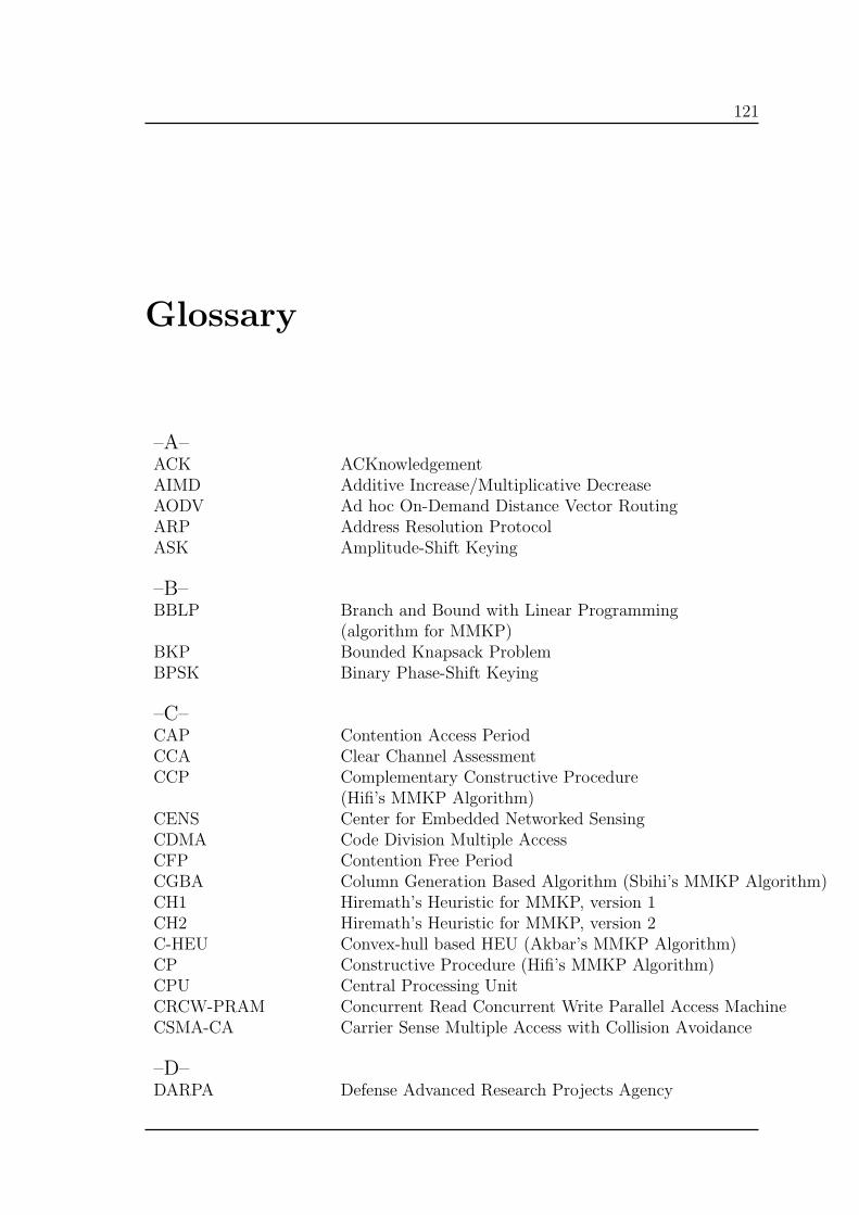
121

Glossary

–A–ACK ACKnowledgementAIMD Additive Increase/Multiplicative DecreaseAODV Ad hoc On-Demand Distance Vector RoutingARP Address Resolution ProtocolASK Amplitude-Shift Keying

–B–BBLP Branch and Bound with Linear Programming

(algorithm for MMKP)BKP Bounded Knapsack ProblemBPSK Binary Phase-Shift Keying

–C–CAP Contention Access PeriodCCA Clear Channel AssessmentCCP Complementary Constructive Procedure

(Hifi’s MMKP Algorithm)CENS Center for Embedded Networked SensingCDMA Code Division Multiple AccessCFP Contention Free PeriodCGBA Column Generation Based Algorithm (Sbihi’s MMKP Algorithm)CH1 Hiremath’s Heuristic for MMKP, version 1CH2 Hiremath’s Heuristic for MMKP, version 2C-HEU Convex-hull based HEU (Akbar’s MMKP Algorithm)CP Constructive Procedure (Hifi’s MMKP Algorithm)CPU Central Processing UnitCRCW-PRAM Concurrent Read Concurrent Write Parallel Access MachineCSMA-CA Carrier Sense Multiple Access with Collision Avoidance

–D–DARPA Defense Advanced Research Projects Agency

122 Glossary

Der Algo Derived Algorithm (Hifi’s MMKP Algorithm)DIS the DIStributed algorithm for max-min fairnessDoD Department of DefenseDSN Distributed Sensor Network

–E–EMKP Exact algorithm for MMKP (Sbihi’s Algorithm)

–F–FDMA Frequency-Division Multiple AccessFFD Full Functional DeviceFLTS First Level Tabu Search (Hiremath’s MMKP Algorithm)

–G–GLPK GNU Linear Programming KitGLS Geographic Location ServiceGPS Global Positioning SystemGTS Guaranteed Time Slot

–H–HEU HEUristic Algorithm for MMKP (Khan’s Algorithm)HMMKP Heuristic for MMKP (Parra-Hernandez’s Algorithm)

–I–IEEE Institute of Electrical and Electronics EngineersI-HEU Incremental HEU (Akabar’s MMKP Algorithm)ISM Industrial, Scientific and Medical

–K–KP Knapsack Problem

–L–LOCAL the LOCAL algorithm for max-min fairnessLP Linear ProgrammingLP-WPAN Low Power Wireless Personal Area Network

–M–MAC Media Access ControlMEMS Micro-Electro-Mechanical SystemMCKP Multiple Choice Knapsack ProblemMDKP Multiple Dimension Knapsack ProblemM-HEU Modified HEU algorithm (Akabar’s MMKP Algorithm)MIP Mixed Integer ProgrammingMKP Multiple Knapsack ProblemMMF Max min Fairness

123

MMKP Knapsack ProblemMNU Max Network UtilityMRLS Modified Reactive Local Search (Hifi’s MMKP Algorithm )MSE Mean Squared ErrorMVRC Maximizing Value per Resource Consumption heuristic

(Chantzara’s MMKP Algorithm)

–N–NACK Negative ACKnowledgementNIB Network Information BaseNP Non-deterministic PolynomialNSF National Science FoundationNWK NetWorK (layer)

–O–OPT the OPTimal algorithm for max-min fairnessOR Operations Research

–P–PAN Personal Area NetworkPDA Personal Digital AssistantPHY PHYsical (layer)

–Q–QoS Quality of ServiceQPSK Quadrature Phase-Shift Keying

–R–RFD Reduced Functional DeviceRLS Reactive Local Search (Hifi’s MMKP Algorithm)

–S–SEM Standard Error of the Mean

–T–TCP Transmission Control ProtocolTDMA Time-Division Multiple AccessTTDD Two-Tier Data Dissemination

–U–

–V–VLSI Very-Large-Scale IntegrationVoD Video on Demand

124 Glossary

–W–WSN Wireless Sensor Networks

–Z–ZC ZigBee ControllerZED ZigBee End DeviceZR ZigBee Router