alkf - irc · influence of the interest rate on the break-even prices ... us $ 0.25/1 for diesel...
TRANSCRIPT

AlKf STEERING COMMITTEE ON WIND-ENERGY FOR DEVELOPING COUNTRIES (Stuurgroep Wind-energie Ontwikkelingslanden)
P.O. BOX 85 / AMERSFOORT / THE NETHERLANDS
international A f e , ) - C'^rr
1323-T8co

\0ob
ZS2-3
COST COMPARISON OF WINDMILL AND ENGINE PUMPS
By L. Marchesini and S.F. Postma
tf&-:ffi£,::s:Vi: §7?:r.-z?. Contrc %i lxv<:ii>':.h: iVstsr Supply
SWD Steering Committee for Windenergy in Developing Countries P.O. Box 85/Amersfoort/The Netherlands Tel. 33/689111 cable dehave Amersfoort, telex 79348 dhv nl

PUBLICATION SWD 7 7 - 2
This publication was realized under the auspices of the Steering Committee on Wind-energy for Developing Countries S.W.D., by DHV, Consulting Engineers, Amersfoort.. The S.W.D. is financed by the Netherlands Ministry for Development Cooperation and is staffed by:
the Eindhoven University of Technology, the Twente University of Technology, the Netherlands Organization for Applied Scientific Research, and DHV, Consulting Engineers, Amersfoort
and collaborates with other interested parties.
The S.W.D. tries to help governments, institutes and private parties in the Third World, with their efforts to use wind-energy and in general to promote the interest for wind-energy in Third World Countries.

2
CONTENTS PAGE
SUMMARY
1. SUMMARY OF THE IRRIGATION EXAMPLE 9
1.1. Introduction 9 1.2 Size of Windmill and Reservoir 9 1.3. Break-even Analysis 9
2. GENERAL MODEL 12
2.1. Introduction 12 2.2. The Model 12 2.3. Sizing-Probleras 15 2.3.1. introduction 15 2.3.2. available energy from windmill pump set 16 2.3.3. required energy for water lifting 17 2.3.4. windmill diameter 17 2.3.5. reservoir capacity 18 2.4. Sensitivity Analysis 18 2.4.1. investment level and lifetime 18 2.4.2. operation and maintenance 18 2.4.3. interest rate 18
3. CALCULATION EXAMPLE 19
3.1. Introduction 19 3.2. Basic Data and Assumptions 19 3.2.1. data on windspeed and distribution 19 3.2.2. water requirements 19 3.2.3. groundwater depth and pumping head 20 3.2.4. efficiency 21 3.3. Determination of Windmill Diameter 21 3.4. Determination of Reservoir Capacity 22 3.5. Considerations on the Calculation Example 25 3.5.1. introduction 25 3.5.2. the influence of wind speed distribution and pumping
head on the size of the windmill 25 3.5.3. the windmill diameter 27 3.5.4. the relation windmill diameter to reservoir capacity 27 3.5.5. the capacity of the reservoir 28 3.5.6. conclusion 32 3.6. Break-even Analysis 33 3.7. Economic Comparison 34 3.8. Sensitivity Analysis on the Break-even Prices of Energy 37
3
CONTINUATION
3.8.1. 3.8.2.
3.8.3.
3.8.4.
3.8.5.
introduction sensitivity to variation pump set sensitivity to variation the windmill pump set sensitivity to variation windmill pump set sensitivity to variation
of investment in windmill
of technical life time of
of maintenance costs of the
of interest rate
PAGE
37
37
40
40 50

4
List of tables
Table S.l. Windmill/reservoir combinations supplying water with the same reliability as the motor pump sets
Table S.2. Cost elements of the windmill alternatives and the motor pump sets
Table S.3. Break-even water volumes of windmill alternatives
Table 2.1. Form for cost comparison of water pumping by windmills and other engines
Table 3.1. Windspeed distribution as registered for month 1, 1976 at Hambantota (Sri Lanka)
Table 3.2. Monthly water requirements of 1 hectare of crops
Table 3.3. Calculation of the required windmill diameter
Table 3.4. Daily useful wind distribution for the critical month
Table 3.5. Calculation method required reservoir
Table 3.6. Simplified daily useful windspeed distribution alternatives
Table 3.7. Relation windspeed distribution to pumping head and required windmill diameter
Table 3.8. Considerations on required reservoir and windmill diameter
Table 3.9. The base situation
Table 3.10. Base situation annual costs
Table 3.11. Base situation break-even prices for energy
Table 3.12. Break-even water volumes (base situation)
Table 3.13. Investigated alternatives
Table 3.14. Break-even prices as a function of investment level
Table 3.15. Break-even water volumes, windmill pump set US $ 1400
5
Table 3.16. Influence of investment level and technical life time of the windmill pump set on the break-even prices for energy
Table 3.17. Influence of windmill pump set maintenance costs, technical life time and investment level on the break-even prices for energy
Table 3.18. Break-even water volumes as a function of investment and maintenance costs
Table 3.19. Influence of the interest rate on the break-even prices for energy
6
List of figures
Fig. 1 Relation break-even price for energy to outflow
Fig. 2 Relation windmill diameter to required reservoir capacity
Fig. 3 Relation break-even prices to annual useful outflow, base situation
Fig. 4 Break-even price sensitivity for investment level windmill pump set
Fig. 5 Diesel break-even prices as a function of investment level and technical life time windmill pump set at various useful annual outflows
Fig. 6 Petrol break-even prices as a function of investment level and technical life time windmill pump set at various useful annual outflows
Fig. 7 Electricity break-even prices as a function of investment level and technical life time windmill pump set at various useful annual outflows
Fig. 8 Diesel break-even prices as a function of operation and maintenance cost windmill pump set
Fig. 9 Petrol break-even prices as a function of operation and maintenance costs windmill pump set
Fig. 10 Electricity break-even prices as a function of operation and maintenance costs wind mill pump set
Fig. 11 Break-even prices of energy as a function of interest rate

7
Symbols and abbreviations
A__. = annual cost of conventional engine = annual costs of windmill
> CE = conventional engine Cp = power coefficient of windrotor D = diameter of windrotor (m) E = energy (wh or kWh) F = annuity factor g = gravitional constant (9.81 m/s2) H = pumping head I_F = investment of conventional engine Ij-, = investment of windmill i = rate of interest n = number of years lifetime 0 + M = operation and maintenance P = power (W) q = outflow of water (m3/s) Q = total outflow of water (m3) W, = windspeed^duration (hours) WH = windmill H = efficiency of pump r£ = efficiency of transmission tp = density of air (~ 1.25 kg/m3)
conversion
factor = 1 US$ = Dfl 2.20 /Feb. 1978)

8
SUMMARY
In this paper a method is given to compare the costs of irrigation with windmills and with conventional engines (diesel, petrol engines or electric motors). The method results in graphs of break-even prices for fuel or electricity as a function of the annual quantity of irrigation water required. The choice of a windmill then is economically justified if the local prices for fuel a alectricity are higher than the break-even prices.
The necessary calculations of the output of windmills on the basis of windregime data are explained. They are demonstrated in an exampte with wind data from Hambantota in Sri Lanka. In this exampte also the sensitivity of variations of different parameters is analyzed.
For the hasty reader a summary of this example and some of its main conclusions are given below.
9
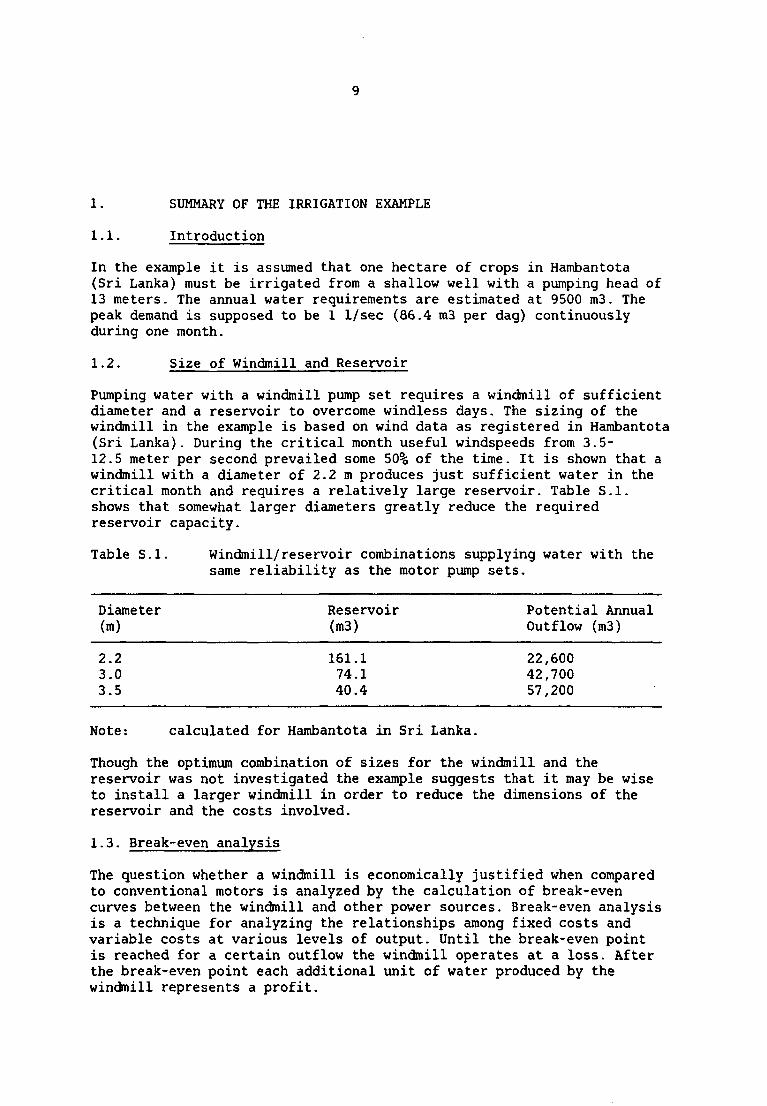
1. SUMMARY OF THE IRRIGATION EXAMPLE
1.1. Introduction
In the example it is assumed that one hectare of crops in Hambantota (Sri Lanka) must be irrigated from a shallow well with a pumping head of 13 meters. The annual water requirements are estimated at 9500 m3. The peak demand is supposed to be 1 1/sec (86.4 m3 per dag) continuously during one month.
1.2. Size of Windmill and Reservoir
Pumping water with a windmill pump set requires a windmill of sufficient diameter and a reservoir to overcome windless days. The sizing of the windmill in the example is based on wind data as registered in Hambantota (Sri Lanka). During the critical month useful windspeeds from 3.5-12.5 meter per second prevailed some 50% of the time. It is shown that a windmill with a diameter of 2.2 m produces just sufficient water in the critical month and requires a relatively large reservoir. Table S.l. shows that somewhat larger diameters greatly reduce the required reservoir capacity.
Table S.l. Windmill/reservoir combinations supplying water with the same reliability as the motor pump sets.
Diameter Reservoir Potential Annual (m) (m3) Outflow (m3)
2.2 161.1 22,600 3.0 74.1 42,700 3.5 40.4 57,200
Note: calculated for Hambantota in Sri Lanka.
Though the optimum combination of sizes for the windmill and the reservoir was not investigated the example suggests that it may be wise to install a larger windmill in order to reduce the dimensions of the reservoir and the costs involved.
1.3. Break-even analysis
The question whether a windmill is economically justified when compared to conventional motors is analyzed by the calculation of break-even curves between the windmill and other power sources. Break-even analysis is a technique for analyzing the relationships among fixed costs and variable costs at various levels of output. Until the break-even point is reached for a certain outflow the windmill operates at a loss. After the break-even point each additional unit of water produced by the windmill represents a profit.
10
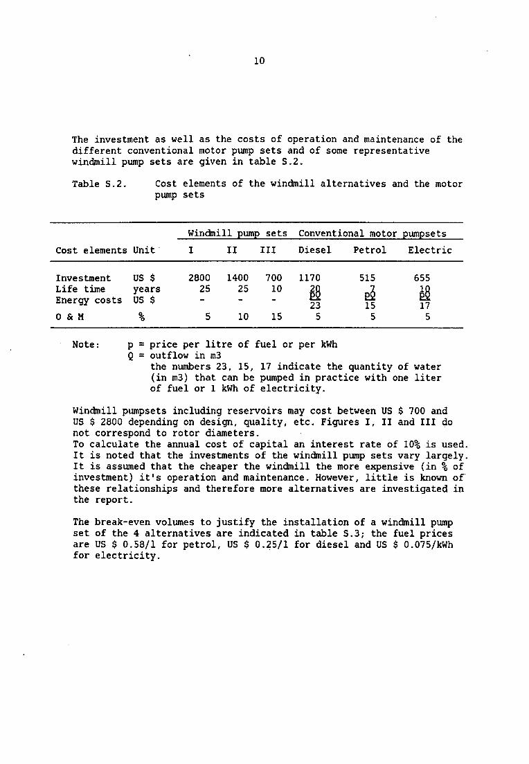
The investment as well as the costs of operation and maintenance of the different conventional motor pump sets and of some representative windmill pump sets are given in table S.2.
Table S.2. Cost elements of the windmill alternatives and the motor pump sets
Cost elements Unit
Windmill pump sets Conventional motor pumpsets
I II III Diesel Petrol Electric
Investment US $ Life time years Energy costs US $
0 & M %
2800 1400 700 1170 25 25 10
10 15 23 5
515
15 5
655
17 5
Note: p = price per litre of fuel or per kWh Q = outflow in m3
the numbers 23, 15, 17 indicate the quantity of water (in m3) that can be pumped in practice with one liter of fuel or 1 kWh of electricity.
Windmill pumpsets including reservoirs may cost between US $ 700 and US $ 2800 depending on design, quality, etc. Figures I, II and III do not correspond to rotor diameters. To calculate the annual cost of capital an interest rate of 10% is used. It is noted that the investments of the windmill pump sets vary largely. It is assumed that the cheaper the windmill the more expensive (in % of investment) it's operation and maintenance. However, little is known of these relationships and therefore more alternatives are investigated in the report.
The break-even volumes to justify the installation of a windmill pump set of the 4 alternatives are indicated in table S.3; the fuel prices are US $ 0.58/1 for petrol, US $ 0.25/1 for diesel and US $ 0.075/kWh for electricity.

11
Table S.3. Break-even water volumes of windmill alternatives windmill pumpsets become attractive when more water than the break even volumes has to be pumped.
(m3/annum)
Conventional alternative
Petrol Diesel Electric
I $ 2800
9,900 23,200 69,900
Windmill pumpsets
II $ 1400
5,100 9,000 35,000
III $ 700
2,700 2,100 17,900
The following conclusions emerge from this table:
For a small scale irrigation project in Hambantota with an annual water demand of 9500 m3 windmills are nearly always cheaper than petrol pump sets. Only the $ 2800 windmill is slightly more expansive than the petrol set.
The higher break-even volumes of diesel pumpsets indicate that they are cheaper than petrol sets. However the $ 1400 and $ 700 type windmills are cheaper (per m3 water pumped) than the diesels.
The still higher break-even values of electric pumpsets indicate that electricity in this case is cheaper than all three windmill alternatives. Windmills only become attractive when more water is needed than the break-even volumes.
It is noted that these conclusions are drawn on the basis of certain energy prices and are valuable only for a specific (and moderately favourable) windspeed distribution. The break-even curves and the simplified formulas in this paper allow the comparison of windmill and conventional power sources for different wind and price information.

12
2. GENERAL MODEL
2.1. Introduction
This paper tries to find an answer to the question of the attractiveness of windmill pump sets compared with their most probable substitutes such as conventional engine driven pump sets.
It compares the cost of energy generated by windmills and conventional prime movers like diesel, petrol and electric engines.
The comparison is executed according to a model which allows to compare investments and recurring annual costs on a single basis.
The model takes into account water supply for irrigation on a small scale as this application is most frequent in developing countries.
Political considerations as well as sociological, cultural and strategical ones, which in practice can heavily influence the decision making process as to what type of pump set should be installed, are not taken into account.
The choice criterion according to which decisions are taken is given by the break-even price for fuel. Break-even analysis is basically a technique for analyzing the relationships between fixed costs and variable costs. Until the break-even point is reached at the intersection of the total cost lines of engine driven pump sets and the windmill pump set, the latter operates at a loss. After the break-even point, each unit of water produced by the windmill represents a profit. The break-even price of fuel at the required outflow rate is compared with the market price for fuel. In case the break-even price which results from the calculation is lower than the market price for fuel, the application of a windmill pump set can be considered favourable.
It should be realised, that the outcome of the comparative analysis depends for an important part on the prevailing wind conditions on the one hand, as well as on the local prices for fuel and the useful annual outflow of the pump set on the other hand.
2.2. The Model
The model is limited to the comparison of those aspects that nececessari-ly differ between windmill and other power source driven pump sets (see table 2.1.). Costs related to the construction of the well and piping system to reach the land to be irrigated are left out of the investigation as these costs are the same for all sources of power.
It is noted that some items are applicable only to the windmill, e.g., tower construction and reservoir. The reservoir is included to allow for comparison of the windmill pump set with conventional engine driven pump sets at the same level of confidence with a view to water supply.

13
Table 2.1. Form for cost compasion of water pumping by windmills and other engines
Windmill (WM)
windmill + tower pump reservoir installation operation and maintenance
Total
Conventional Engine (CE)
prime mover pump installation operation and maintenance
Total
Investment
(N.A.)
IWM
Investment
(N.A.)
:CE
Annual Costs
*WM
Annual Costs (without fuel costs)
ACE
Note: N.A. = Not Applicable.
C. Calculated useful quantity of irrigation water: m3 Local price of petrol
dieseloil electricity
In order to make investments with different life time comparable to annual costs like operation and maintenance, the investments are converted into an annual equivalent, the so called annuity. This annual equivalent includes depreciation and interest and is obtained by means of annuity factors, which can be calculated by the following formula: In annex .. one finds some annuity tables.
It will be clear that windmills are economically attractive if its annual costs are lower than the annual costs of the conventional engine

14
included its fuel costs:
*»! < ACE+ Afuel in which:
. , , price of 1 liter fuel , ... A fuel = r . -i rr- ^—r x annual quantity
outflow per liter fuel In the break-even analysis the price of 1 liter of fuel is calculated for which the annual costs of windmills and of conventional engines are equal:
*WM = ACE + Afuel or:
price of 1 liter fuel = (A^ - ACE) x totfl^nnual^uantitj1
F =
in which F = annuity factor i = interest n = technical life time (years)
i (1 + i)"
(1 + Dn-1
The resulting pf , is the break-even price of one liter of fuel. In case of electricupump set the break-even price is given per kWh.
i

15
Fig. 1 shows the general shape of a curve resulting from the described break-even analysis.
This presentation is a useful yardstick to determine whether the windmill pump set has an advantage over conventional engine driven pump sets at the running prices for energy.
FIG. 1 RELATION BREAK-EVEN PRICE FOR ENERGY TO OUTFLOW
0 5000 Annual uieful outflow (m3) -»•
10000 15000 20000
It is noted however that different windspeed regimes result in different break-even curves as they influence the required size of the windmill diameter, windmill tower construction and reservoir capacity and thus the required investments.
2.3. Sizing-Problems
2.3.1. introduction
Before an economic comparison can be made the windmill and the conventional pump sets should be sized according to water requirements. This problem may be solved by taking the water availability of a well as the basis.

16
In case the availability of water does not form a constraint, the size of the area to be irrigated and the water requirement of the crops may be taken as a starting point. In the calculation example it is assumed that the (shallow) well has enough capacity to irrigate one hectare of land.
2.3.2. available energy from windmill pump set
The power produced by a windmill pump set depends on wind speed, windmill diameter and the efficiency in combination with a pump, as defined by the following formula:
p = \ a v3 ̂ D 2 c n*. n (w) 2 4 p 't p v '
P = available (mechanical) power (W) p = density of air (kg/m3) V = windspeed (m/s) D = diamater of windrotor iy) Cp = power coefficient of windrotor (-) r)t = efficiency of transmission (-) HP = efficiency of pump (-) For each windspeed interval the corresponding power can be calculated by taking the average windspeed of the interval: V =3.5 m/s for the interval between 3 and 4 m/s, etc.
The energy generated by the windmill can be calculated for each interval by multiplying the power found above with the duration of that interval, i.e. the number of hours that the wind had a speed within the interval:
E = P.Wd (Wh) (2) in which: E = energy (Wh) P = power (W) W, = windspeedduration (hours)
The total energy generated is the sum of all fractions generated at each interval:
V=z
i h s , . v3 . |̂ . D 2 • cp nt np _ wd (wh) (3)
in which a and 2 are respectively the lower and upper mind speed limits between which the windmill operates.

17
2.3.3. required energy for water lifting
The energy required to lift the water depends on the pumping head, the required quantity of water to be pumped and the gravitation according to the following formula, in which the mass of water is assumed at 1 gram/cm3:
F = o - q - H (wh) (4) R 3.6
in which: E = Energy required (Wh) Q = quantity of water (m3) g =9.81 (m/sec2) H = head (m)
The required power to be installed is calculated according to:
p = q - 9 - H (W) (5) R
in which: P = power required (W) q = outflow rate (1/sec) g =9,81 (m/sec2) H = head (m)
2.3.4. windmill diameter
The windmill pump set should be able to meet water requirements during any month given the wind distribution.
Therefore the windmill should be sized bearing in mind that for every . month the following equation should at least be fulfilled:
Total energy required Total energy available for water lifting = for water lifting
(6) (in Wh) (in Wh)
Given a fixed wind distribution, pumping head, air density and windmill pump set efficiencies this means that according to formula (4) and formula (3) the windmill diameter can be calculated by solving D from the equation.
The calculation of the diameter should be executed for each month on the hand of the corresponding water requirement and wind distribution data.
The calculations result in various diameters of which the largest should be taken.

18
2.3.5. reservoir capacity
The energy available for pumping purposes generated by a windmill pump set depends on the wind speed and its duration and is therefore not firm.
In order to be comparable to pumping with conventional engine driven sets the windmill pump set should include a reservoir to overcome calm days.
The dimension of the reservoir is based on the water requirements and the daily wind fluctuations during the critical month, which is the month in which the diameter required by the windmill to fulfill water demand under the given wind regime is set at its maximum value. Other criteria such as equalisation of marginal costs (for windmill diameter increase and risk of crop failure) and marginal benefits (deriving from the reduction in reservoir capacity) are considered, but not worked out in detail as this would require laborious information on cropping patterns, crop response to water gifts and on market prices (all items which are beyond the scope of this paper).
2.4. Sensitivity Analysis
2.4.1. investment level and life time
Prices of windmill pump sets may vary considerably from one country to another. Also the probable technical life time of different designs and construction methods is largely unknown. Therefore sensitivity to variation in investment and life time should be tested.
2.4.2. operation and maintenance
Costs of maintenance are estimated on a percentage basis of the investment. Presently no reliable data are available on these costs for windmill pump sets. Therefore the influence of variation of these costs is also tested.
2.4.3. interest rate
The basic interest rate to be included in the economic comparison among technical alternatives is generally taken as the opportunity cost of capital. As this can vary in different countries because of marginal investment opportunities (national economic point of view) or market rate for interest (private point of view), the influence of deviation from this basic interest rate will also be evaluated.

19
3 . CALCULATION EXAMPLE
3.1. Introduction
The calculation example is based on the elaboration of a small scale irrigation project. The data concerning windspeed and their distribution are taken from windspeed records registered in Hambantota (Sri Lanka) over a period of one year (July 1975 - June 1976).
The prices of conventional pump sets refer to those prevailing in The Netherlands. The life time of the various engines is estimated on the basis of practical experience.
The cost of a windmill pump set varies considerably with the materials used, the costing procedure and the design.
The relation between the investment level of windmill pump sets and the technical life time as well as the operation and maintenance costs is unknown.
However assumptions are made on these subjects.
3.2. Basic Data and Assumptions
3.2.1. data on windspeed and distribution
In table 3.1. an example of the windspeed data underlying the calculation is given for one month.
3.2.2. water requirements
As the model will be applied to small scale irrigation of agricultural . crops it is assumed that water will be taken from a shallow well. The water that can be pumped from this well is assumed to be sufficient for the irrigation of 1 ha of crops. The peak requirement of these crops is set at 1 liter/second during 24 hours for one month, equivalent to 8.6 mm/day. The resulting water requirement of the peakmonth and assumptions on requirements during the other months of the growing season are indicated in table 3.2. (the requirements refer to 1 crop a year).
Table 3.2. Monthly water requirements of 1 hectare of crops (m3)
Month March April May June July August Sept Year Total
535 1036 1607 2592 1607 1607 518 9502

20
3.2.3. groundwater depth and pumping head
The average groundwater level in the shallow well is assumed to be at 13 meters below surface. The head for the conventional engine driven pump sets therefore is 13 meters. For the windmill pump sets 15 m is taken in view of the waterdepth in the reservoir.

21
3.2.4. efficiency
According to formula (3) only part of the wind energy can be transformed by the windmill and used for pumping purposes. The coefficients which influence the available power and energy are indicated in formula (1) and (3); they are the air density factor (p), the power coefficient (C ) of the windmill rotor and the pumping and transmission efficiencies " (resp. n and r\ ). Though the values of these items vary from place to place ( and should be measured on the spot for exact calculations) this paper takes into account the following figures:
C x P
^air n
"P X
\ —
=
=
0.
1.
3
.16
.250
.14
Formula (1) therefore can be reduced to:
P = 0.078 V3 D2 (W) (8)
Formula (3) can be reduced to:
E = ZP.Wd = I 0.078 V 2 D2 W d (wh) (g)
3.3. Determination of the Windmill Diameter
The windmill should be sized in such a way that the monthly available energy at least meets the monthly required energy for lifting water. The windmill diameter can be calculated by solving D from the following equation
Energy required Energy available for for water lifting = water lifting (in Wh) (in Wh)
or
<* x s:8l x 15 = ViYo78 v3 D 2 w„ (io) B 3.6
•) n = / Q 40-87
V=a
D = V I 0.078 V3 D2 W
or
d
V=z I
V=a
Q = 0.0019 I VJ Wd D (m ) (11)

22
In principle the diameter must be calculated for each month using the monthly water requirement and wind speed distribution data.
The results of the calculation are shown in the following table.
Table 3.3. Calculation of Required Windmill Diameter
Energy Required Energy Resulting Month available water required diameter
(kWh) (m3) (kWh) (meter)
535 21.87 2.02 1036 42.35 2.20 1607 65.69 1.60 2592 105.95 1.88 1607 65.69 1.89 1607 65.69 1.76 518 21.17 1.02
Total 190.89 x D 9502 388.41
Potential water supply: approx 22600 m3 (based on a diameter of 2.2 m)
It follows from table 3.3. that in order to meet monthly water requirements at any time the windmill diameter should be set at 2.20 meter (the windmill diameter as calculated for month 4).
Introduction of this diameter in the total energy available equation shows that the potential water supply by the windmill pumpset largely exceeds the required annual volume of 9502 m3. The total annual potential water supply (assuming the capacity of the well is no constraint) is about 22600 m3.
3.4. Determination of the Reservoir Capacity
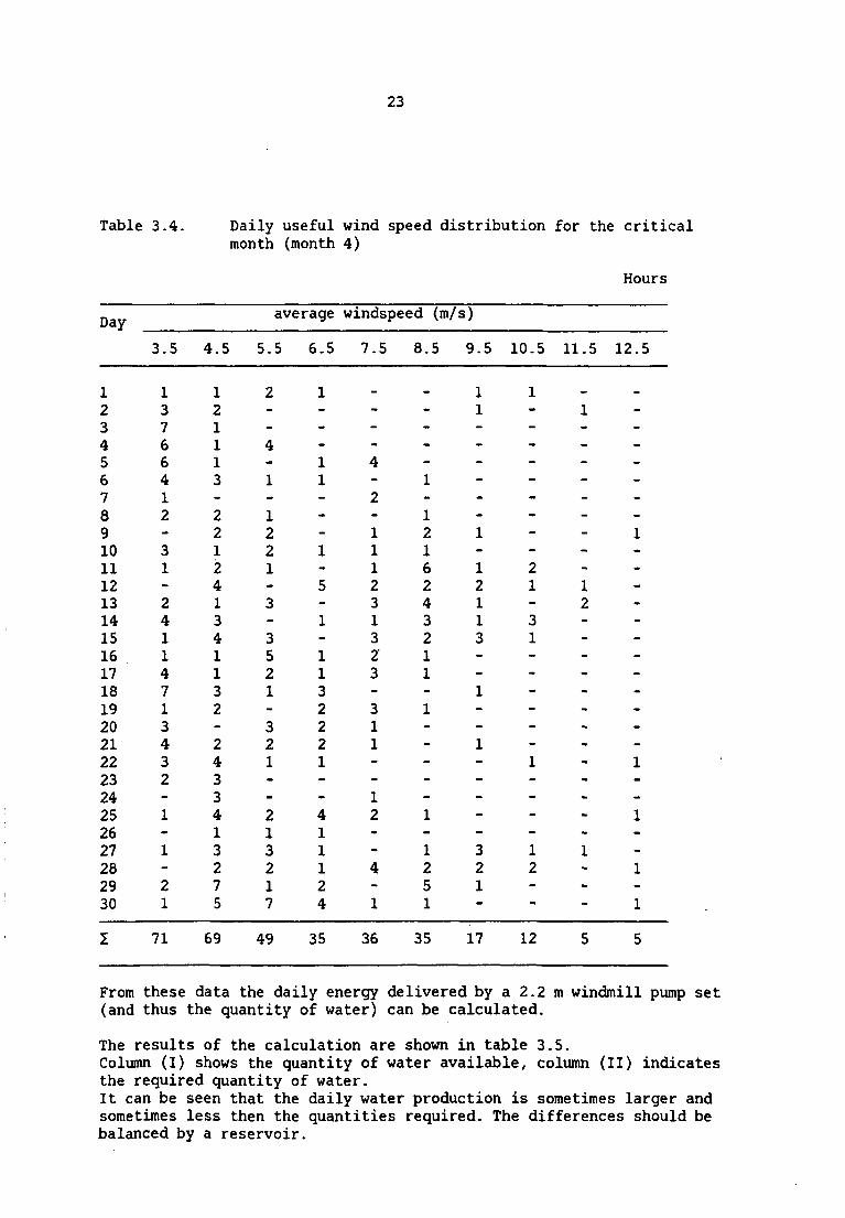
The calculation of the reservoir capacity is based on daily wind distribution data of month 4, as shown in table 3.4.
1 2 3 4 5 6 7 8 9 10 11 12
14.36 x 11.15 X 5.35 X 8.69 x 25.75 X 29.90 x 18.44 X 21.15 x 20.11 x 18.90 x 7.87 x 9.22 X
23
Table 3.4. Daily useful wind speed distribution for the critical month (month 4)
Hours
Day
1 2 3 4 5 6 7 8 9 10 11 12 13 14 15 16 17 18 19 20 21 22 23 24 25 26 27 28 29 30
I
3.5
1 3 7 6 6 4 1 2 -
3 1 -
2 4 1 1 4 7 1 3 4 3 2 -
1 -
1 -
2 1
71
4.5
1 2 1 1 1 3 -
2 2 1 2 4 1 3 4 1 1 3 2 -
2 4 3 3 4 1 3 2 7 5
69
ave
5.5
2 --
4 -
1 -
1 2 2 1 -
3 -
3 5 2 1 -
3 2 1 --
2 1 3 2 1 7
49
>rage
6.5
1 ---
1 1 ---
1 -
5 -
1 -
1 1 3 2 2 2 1 --
4 1 1 1 2 4
35
windspeed (m/:
7.5
_
---
4 -
2 -
1 1 1 2 3 1 3 2 3 -
3 1 1 --
1 2 --
4 -
1
36
8.5
»
----
1 -
1 2 1 6 2 4 3 2 1 1 -
1 -----
1 -
1 2 5 1
35
s)
9.5
1 1 ------
1 -
1 2 1 1 3 --
1 --
1 -----
3 2 1 -
17
10.5
1 ---------
2 1 -
3 1 ------
1 ----
1 2 --
12
11.5
_
1 ---------
1 2 -------------
1 ---
5
12.5
_
-------
1 ------------
1 --
1 --
1 -
1
5
From these data the daily energy delivered by a 2.2 m windmill pump set (and thus the quantity of water) can be calculated.
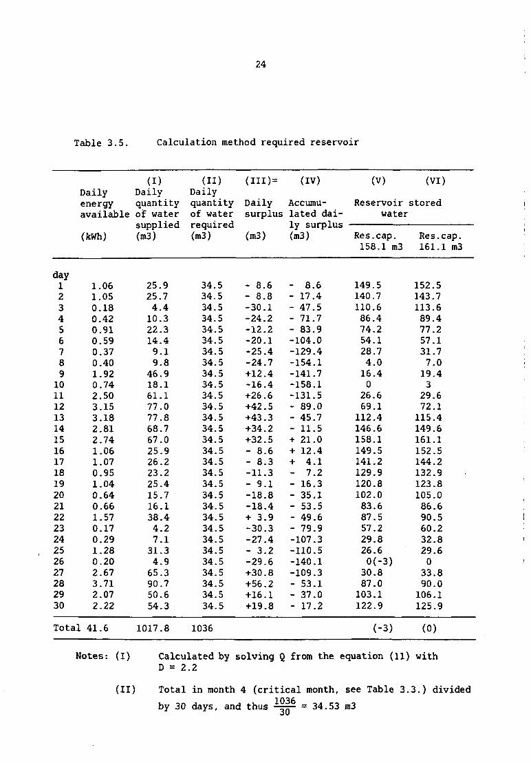
The results of the calculation are shown in table 3.5. Column (I) shows the quantity of water available, column (II) indicates the required quantity of water. It can be seen that the daily water production is sometimes larger and sometimes less then the quantities required. The differences should be balanced by a reservoir.
24
Table 3.5. Calculation method required reservoir
day 1 2 3 4 5 6 7 8 9 10 11 12 13 14 15 16 17 18 19 20 21 22 23 24 25 26 27 28 29 30
Daily energy available
(kWh)
1.06 1.05 0.18 0.42 0.91 0.59 0.37 0.40 1.92 0.74 2.50 3.15 3.18 2.81 2.74 1.06 1.07 0.95 1.04 0.64 0.66 1.57 0.17 0.29 1.28 0.20 2.67 3.71 2.07 2.22
Total 41.6
(I) Daily quantity of water supplied (m3)
25.9 25.7 4.4 10.3 22.3 14.4 9.1 9.8 46.9 18.1 61.1 77.0 77.8 68.7 67.0 25.9 26.2 23.2 25.4 15.7 16.1 38.4 4.2 7.1 31.3 4.9 65.3 90.7 50.6 54.3
1017.8
(II) Daily quantity of water required (m3)
34.5 34.5 34.5 34.5 34.5 34.5 34.5 34.5 34.5 34.5 34.5 34.5 34.5 34.5 34.5 34.5 34.5 34.5 34.5 34.5 34.5 34.5 34.5 34.5 34.5 34.5 34.5 34.5 34.5 34.5
1036
(IH)=
Daily surplus
(n>3)
- 8.6 - 8.8 -30.1 -24.2 -12.2 -20.1 -25.4 -24.7 +12.4 -16.4 +26.6 +42.5 +43.3 +34.2 +32.5 - 8.6 - 8.3 -11.3 - 9.1 -18.8 -18.4 + 3.9 -30.3 -27.4 - 3.2 -29.6 +30.8 +56.2 +16.1 +19.8
(IV)
Accumulated daily surplus (m3)
- 8.6 - 17.4 - 47.5 - 71.7 - 83.9 -104.0 -129.4 -154.1 -141.7 -158.1 -131.5 - 89.0 - 45.7 - 11.5 + 21.0 + 12.4 + 4.1 - 7.2 - 16.3 - 35.1 - 53.5 - 49.6 - 79.9 -107.3 -110.5 -140.1 -109.3 - 53.1 - 37.0 - 17.2
(V)
Reservoir water
Res.cap. 158.1 m3
149.5 140.7 110.6 86.4 74.2 54.1 28.7 4.0 16.4 0 26.6 69.1 112.4 146.6 158.1 149.5 141.2 129.9 120.8 102.0 83.6 87.5 57.2 29.8 26.6 0(-3) 30.8 87.0 103.1 122.9
(-3)
(VI)
stored
Res.cap. 161.1 m3
152.5 143.7 113.6 89.4 77.2 57.1 31.7 7.0 19.4 3 29.6 72.1 115.4 149.6 161.1 152.5 144.2 132.9 123.8 105.0 86.6 90.5 60.2 32.8 29.6 0 33.8 90.0 106.1 125.9
(0)
Notes-. (I) Calculated by solving Q from the equation (11) with D = 2.2
(II) Total in month 4 (critical month, see Table 3.3.) divided
by 30 days, and thus 1036 30
= 34.53 m3

25
(III) Daily surplus: Quantity of water supplied (I) - Quantity of water required (II)
(IV) Cumulation of daily surpluses as given in column (III)
(V) Reservoir stored quantity of water is based on a start with a full reservoir, dimensioned as given by the minimum figure in column (IV)
(VI) Reservoir stored based on col. V, increased in capacity with 3 cubic meters
Rounding of windspeeds to the nearest half resulted in an error of one percent in the energy available and thus in the quantities delivered.
The capacity of the reservoir is determined by trial and error along the following steps. First take the largest cumulated deficit (table 3.5. col. IV: 158.1 m3 in day 10) and calculate the reservoir operations starting with a reservoir completely filled up (col. V).
The calculation shows that there still is a deficit (shown by the figure in brackets) of 3 m3 in day 26 which should be avoided in order to make the windmill pump set strictly comparable to conventional engine driven pump sets. Therefore the capacity of the reservoir should be increased with 3 m3 to 161.1 m3.
3.5. Considerations on the Calculation Example
3.5.1. introduction
In the following paragraphs simplified examples of various
windspeed distributions pumping heads
are given in order to demonstrate the influence on the calculations assuming a daily water requirement of 86.4 m3 in the peak month (2592 m2 in month 6, see table 3.3). Furthermore some considerations on the sizing problem, as executed on the basis of the Hambantota windspeed data, are worked out with special attention to the sizing of the windmill diameter and the reservoir (par. 3.5.3. to 3.5.5.).
3.5.2. the influence of windspeed distribution and pumping head on
the size of the windmill
In the following examples it is assumed that useful windspeeds prevail during 12 hours a day, so 50% of the time. Table 3.6. indicates 3 simplified examples of windspeed distributions (1), (2) and (3).

26 j i
Table 3.6. Simplified daily useful windspeed distribution alternatives
(m/s)
Windspeed durat (hours/day)
4 4 4
Average useful speed
:ion
wind-
Windspeed distribution
(1)
3.5 4.5 5.5
4.5
(2)
4.5 5.5 6.5
5.5
(3)
5.5 6.5 7.5
6.5
Introduction of the water quantity, the windspeeds and their duration into the equation:
Energy required = Energy delivered
or, 0.235 x H = I 0.079 x V3 x Wd x D2
in which H stands for pumping head, V for windspeed, Wd for windspeed duration and D for diameter. This results in the daily energy available (kWh) and the required windmill diameters for 3 different pumping heads as indicated in table 3.7.
Table 3.7. Relation windspeed distribution to pumping head and required windmill diameter (based on a water demand of 86.4 m3/day)
Windspeed distribution
(1) (2) (3)
Available energy (kWh) '• 0.0949 D 0.1682 D 0.2727 D
pumping head Required v Required diameter (m) (H in meters) energy (kWh) '
15 m 3.525 6.10 4.58 3.60 10 m 2.350 4.98 3.74 2.94 5 m 1.175 3.53 2.65 2.08
Daily energy
It is noted that the diameters for 15, 10 and 5 m pumping head are related to each other by the square root of the ratio of the pumping heads.

27
For instance, pumping from 10 in stead of 5 m depth requires twice as much energy resulting in a windmill diameter of ̂ 2 times larger. The available energy has the same relation, e.g., the energy under the windspeed distribution as«prevailing under alternative 1 to alternative 2 increases from 0,0949 D to 0.1682 D , or by a factor 1.77. The diameter capable to deliver the same amount of energy under windspeed distribution 2 can be obtained by dividing the one as resulting from the windspeed distribution 1 by ̂ 1-77 or 1.33.
3.5.3. the windmill diameter
The sizing of the windmill was discussed in paragraph 3.3. The calculation resulted in a windmill diameter of 2.2 m given the specific environmental circumstances (windspeed distribution, pumping head of 15 m).
Despite this calculation it is reasonable to assume that manufacturers who produce windmills on a large (industrial) scale standardize their products.
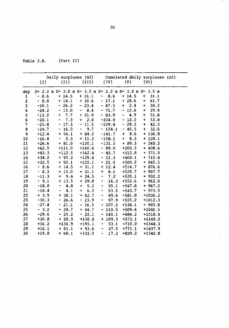
In the following the operation of a windmill of 3.0 m and 3.5 m diameter is evaluated and compared to the windmill with a diameter of 2.2 m.
Table 3.8., part I, column (I) to (VI) shows the energy available for pumping purposes and the quantities of water pumped.
It is worth noting that once the complete calculation is executed for a specific windmill diameter the corresponding figures for other diameters can be found by multiplication of the calculated figures with the ratio of the squares of the windmill diameters.
For the windmill with a rotor of 3.5 m diameter the multiplication factor, taking,,the figures of the 2.2 m windmill as the base, showed to be (3.5r/2.2) or 2.53.
An increase in windmill diameter from 2.2 m to respectively 3.0 m and 3.5m results in a considerable increase in water supply as shown by the total figures in table 3.8, part I (page 27).
3.5.4. the relation windmill diameter to reservoir capacity
The calculation of the reservoir capacity required by the windmill pump set system in order to supply water with the same level of confidence as the conventional engine driven pump sets was shown in paragraph 3.4. for a windmill with a rotor diameter of 2.2 m (reservoir of 161.3 m3).
The reservoir can be calculated according to the same procedure for the windmills with rotor diameters of 3,0 m and 3.5 m.
Based on the intermediate results of table 3.8., part II, part III shows the reservoir as required in these latter cases (col. II and col. Ill) as well as the reservoir required for the 2.2 m windmill (col. I).

28
It can be seen that increasing the windmill diameter from 2.2 m to 3.0 m and 3.5m has a reducing effect on the required reservoir. The reservoir decreases from 161.1 m3 to respectively 74.1 m3 and 40.4 m3. It is quite possible that this will reduce the total cost of windmill plus reservoir.
3.5.5. the capacity of the reservoir
In the calculation example of paragraph 3.4. a 2.2. m windmill pump set requires a reservoir of 161.1 m3. If the reservoir would be reduced to 80 m3 without increasing the windmill diameter a deficiency of 107.1 m3 will occur. A reservoir of 40 m3 causes a dificiency of 176.0 m3 (see Table 3.8., part III, column IV and V). These difficiencies are calculated as follows:
irrigation takes place twice a month; this implies 15 plots, irrigated at intervals of 15 days when the reservoir fails, part of the area cannot be irrigated, the crop will fail and further irrigation after 15 days is not worthwhile. Hence, the waterrequirement is reduced by the part of the area that fails in the first half of the month
In case the reservoir is reduced to 80 m3 a deficiency of 107.1 m3 occurs (table 3.8., part III, col. IV). This may result in damage to the crop. The damage may be estimated by determining the area reduction on the basis of deficiencies in water supply during the first irrigation (the first 15 days of the month). The water requirements for the second half of the month must be reduced accordingly. The area reduction as a result of deficiency in first irrigation is of (3.9 + 20.1 + 25.4 + 24.7)/34.5 x 1/15 or about 14% of the area irrigated.
An additional reduction in cropped area is caused by a deficiency in water supply on the 26th day, being 29.0 m3. This deficit which occurs during the second irrigation period can cause a crop loss of at maximum 29/34.5 x 1/15 or 6% of the area irrigated. The total area reduction due to a decrease of the reservoir capacity from 161.1 m3 to 80 m3 is therefore 14% + 6% = 20% of the cropped area.
In case of a reservoir of 40 m3 (table 3.8., part III, col. (V)) the water deficiency during the first half of the month is 118.1 m3, which causes a reduction in cropped area of 118.1/34.5 x 1/15 or 23%. A further reduction caused by insufficient second watering reduces the crop area once more by at maximum (1.7 + 27.4 + 28.8)/34.5 x 1/15 or some 11%. The total maximum area reduction in this case is 23% + 11% = 34% of the cropped area.

29
Table 3.8. (Part I) Consideration diameter
Energy available for pumping water
(I) (ID
day D= 2.2 m D= 3.0 m D 1 2 3 4 5 6 7 8 9 10 11 12 13 14 15 16 17 18 19 20 21 22 23 24 25 26 27 28 29 30
Total Total
1.06 1.05 0.18 0.42 0.91 0.59 0.37 0.40 1.92 0.74 2.50 3.15 3.18 2.81 2.74 1.06 1.07 0.95 1.04 0.64 0.66 1.57 0.17 0.29 1.28 0.20 2.67 3.71 2.07 2.22
volume annual
1.97 1.95 0.33 0.78 1.69 1.12 0.70 0.76 3.63 1.40 4.73 5.95 6.01 5.31 5.18 2.00 2.02 1.80 1.97 1.21 1.25 2.97 0.32 0.55 2.42 0.38 5.05 7.01 3.91 4.20
month 4 volume
(kWh)
(III)
= 3.5 m 2.68 2.65 0.45 1.84 2.30 1.52 0.95 1.03 4.94 1.90 6.43 8.09 8.17 7.22 7.04 2.72 2.75 2.45 2.68 1.65 1.70 4.04 0.44 0.75 3.29 0.52 6.87 9.53 5.35 5.71
on required reservoir and windmill
Quantity of water supplied (m3)
(IV)
D= 2.2 25.9 25.7 4.4 10.3 22.3 14.4 9.1 9.8 46.9 18.1 61.1 77.0 77.8 68.7 67.0 25.9 26.2 23.2 25.4 15.7 16.1 38.4 4.2 7.1 31.3 4.9 65.3 9.7 50.6 54.3
1017.8 22600
(V)
m D= 3.0 49.0 48.6 8.3 19.5 42.2 27.2 17.2 18.5 88.6 34.2 115.5 145.5 147.0 129.8 126.6 49.0 49.5 43.9 48.0 29.7 30.4 72.6 7.9 13.4 59.2 9.3
123.4 171.4 95.6 102.6
1923.6 42700
(VI)
m D= 3.5 65.6 65.1 11.1 26.1 56.4 36.5 23.0 24.8 118.7 45.8 154.6 194.9 196.9 173.9 169.6 65.6 65.6 58.7 64.3 39.7 40.8 97.2 10.6 18.0 77.2 12.4 165.3 229.6 128.1 137.4
2575.5 57200
Quantity of water required (m3)
(VII)
m 34.5 34.5 34.5 34.5 34.5 34.5 34.5 34.5 34.5 34.5 34.5 34.5 34.5 34.5 34.5 34.5 34.5 34.5 34.5 34.5 34.5 34.5 34.5 34.5 34.5 34.5 34.5 34.5 34.5 34.5
1036 9506
30
Table 3.8. (Part I I )
day 1 2 3 4 5 6 7 8 9 10 11 12 13 14 15 16 17 18 19 20 21 22 23 24 25 26 27 28 29 30
Dai (I)
D= 2.2 m - 8.6 - 8.8 -30.1 -24.2 -12.2 -20.1 -25.4 -24.7 +12.4 -16.4 +26.6 +42.5 +43.3 +34.2 +32.5 - 8.6 - 8.3 -11.3 - 9.1
. -18.8 -18.4 + 3.9 -30.3 -27.4 - 3.2 -29.6 +30.8 +56.2 +16.1 +19.8
ly surpluses (m3)
(ID
D= 3.0 m + 14.5 + 14.1 - 26.2 - 15.0 + 7.7 - 7.3 - 17.3 - 16.0 + 54.1 - 0.3 + 81.0 +111.0 +112.5 + 95.3 + 92.1 + 14.5 + 15.0 + 9.4 + 13.5 - 4.8 - 4.1 + 38.1 - 26.6 - 21.1 + 24.7 - 25.2 + 88.9 +136.9 + 61.1 + 68.1
(III)
D= 3.5 m + 31.1 + 30.6 - 23.4 - 8.4 + 21.9 + 2.0 - 11.5 - 9.7 + 84.2 + 11.3 +120.1 +160.4 +162.4 +139.4 +135.1 + 31.1 + 31.1 + 24.5 + 29.8 + 5.2 + 6.3 + 62.7 - 23.9 - 16.5 + 44.7 - 22.1 +130.8 +195.1 + 93.6 +102.9
Cumulated daily (IV)
D= 2.2 m - 8.6 - 17.1 - 47.5 - 71.7 - 83.9 -104.0 -129.4 - 154.1 -141.7 -158.1 -131.5 - 89.0 - 45.7 - 11.5 + 21.0 + 12.4 + 4.1 - 7.2 - 16.3 - 35.1 - 53.5 - 49.6 - 97.9 - 107.3 - 110.5 - 140.1 + 109.3 - 53.1 - 37.0 - 17.2
(V)
D= 3.0 m + 14.5 + 28.6 + 2.4 - 12.6 - 4.9 - 12.2 - 29.5 - 45.5 + 8.6 + 8.3 + 89.3 +200.3 +312.8 +408.1 +500.2 +514.7 +529.7 +539.1 +552.6 +547.8 +543.7 +581.8 +555.2 +534.1 +509.4 +484.2 +573.1 +710.0 +771.1 +839.2
surpluses (m3) (VI)
D= + + + + + + + + + + + + + + + + + + + + +
3.5 m 31.1 61.7 38.3 29.9 51.8 53.8 42.3 32.6 136.8 128.1 248.2 408.6 571.0 710.4 845.5 876.6 907.7 932.2 962.0 967.2 973.5
+1036.2 +1012.3 + 995.8 +1040.5 +1018.4 +1149.2 +1344.3 +1437.9 +1540.8

31
Table 3.8. (Part III)
Reservoir stored water
(I) (ID (HI) (IV) (V)
Day
1 2 3 4 5 6 7 8 9
10 11 12 13 14 15 16 17 18 19 20 21 22 23 24 25 26 27 28 29 30
D = 2.2 m Res. cap. = 161.1 m3
152.5 143.7 113.6
89.4 77.2 57.1 31.7
7 19.4
3 29.6 72.1 15.4
149.6 161.1 152.5 144.2 132.9 123.8 105.0
86.6 90.5 60.2 32.8 35.6
0 33.8 90
106.1 125.9
D = 3.0 m Res. cap. = 74.1 m3
74.1 74.1 47.9 32.9 40.6 33.3 16.0
0 54.1 53.8 74.1 74.1 74.1 74.1 74.1 74.1 74.1 74.1 74.1 69.3 85.2 74.1 47 .5 26.4 51.1 25.9 74 74.1 74.1 74.1
D = 3.5 m Res. cap. = 40.4 m3
39.7 40.4 17.0 8.6
30.5 32.5 21.0 11.3 40.4 40.4 40.4 40.4 40.4 40.4 40.4 40.4 40.4 40.4 40.4 40.4 40.4 40.4 16.5
0 40.7 18.6 40.7 40.7 40.7 40.7
D = 2. .2 m Res . cap . = 80 m3
71 .4 71.4 32 .5
8.3 0 ( - 3 0( -20 0( -25 0 ( -24 12.4 0 ( - 4 26.6 69 .1 80.0 80.0 80.0 80.0 71.4 63 .1 51.8 46 .6 44 .0 30 .9 34 .1
3 .8 0.6
0( -29 30 .8 80.0 80.0 80.0
•9) •1) • 4 )
•7)
• 0)
• 0 )
D = 2.2 m Res. cap. = 40 m3
31.4 31.4 0 ( - 7 . 5 ) 0 ( -24 .2 ) 0 ( -12 .2 ) 0 ( -20 .1 ) 0 ( -25 .4 ) 0 ( -24 .7 ) 12.4 0 ( - 4 .0) 26.6 40.0 40.0 40.0 40.0 31.4 23 1 III 3-8 26.9 23.0 24.7 28.6 0 ( - 1.7) 0 ( -27 .4 ) + 0 .8 0 ( -28 .8 ) 30 .8 40.0 40.0 40.0
Total deficit (0) (0) (0) (-107.1) (-176.0)

32
3.5.6. conclusion
Once the windspeed distribution and pumping head are known the sizing of the windmill diameter cannot be seen separately from the sizing of the reservoir. The approach of minimising the windmill diameter after which the matching reservoir is calculated does not necessarily result in the least cost alternative. Reductions in the investment level of the windmill may well be offset by the increase in investment required by the reservoir. The calculation example showed the following relation between windmill diameter and reservoir capacity.
FIG. 2 RELATION WINDMILL DIAMETER TO RESERVOIR CAPACITY
reservoir capacity (nv*)
Note: Figure not general applicable. (Bated on Hambantota wind data)
The least-cost combination of the windmill and the reservoir which supplies water at a same level of confidence as the conventional engine driven pump sets can be calculated by trial and error.

33
The windmill diameter may be increased as long as the additional total costs for the windmill are offset by the total additional savings resulting from the smaller reservoir (the totals refer to annual figures).
Once the windmill/reservoir combination as calculated above has been established a further reduction of the reservoir may be allowed. It is obvious that this implies the risk of water deficiency, resulting in crop damage. The reduction however is allowed as long as the total additional savings in construction costs for the reservoir are larger than the total net-income foregone resulting from crop damage.
3.6. Break-even analysis
The base situation for the different pump sets is defined by the following table:
Table 3.9. The base situation
windmill diesel petrol electric pump set pump set pump set pump set
power 0.38 ^ kW 3.5 hp 3 hp 1.20 kW
investment level (US $) life time (years) interest rate
operation and maintenance
energy costs (US $)
2800 25 10%
5%
-
1170 20 10%
5%
E2 2 )
23
515 7
10%
5%
E2 2 )
15
655 10 10%
5%
E22>
17
notes: 1)
2)
power of the windmill is calculated at a windspeed of 10 m/s, windmill diameter 2.2 m p stands for price of fuel. Q stands for total annual useful outflow. In case of the diesel pump set and the petrol pump set the price is given per liter. In case of the electric pump set the price is given per kWh. The numbers 23, 15 and 17 stand for the quantity of water which can be pumped with 1 liter of fuel (diesel and petrol) or with one kilowatthour from a depth of 13 meters.
The investment levels represent the totals of the relevant parts of the water supply system alternative. The investments required by the water distribution system as well as the drilling costs are excluded from these figures.

34
In case of the windmill driven pump sets the investment figure includes the construction of a reservoir. Little consistency exists in the costing methods which are applied for windmills. Construction methods vary considerably from one place to another (from labour intensive to capital intensive).
The analysis is limited to global investment levels without going into detail of the components of the system considered, such as the windmill, the windmill tower, the pump and the reservoir.
The investments required by the windmill pump sets as well as the conventional engine driven sets and their technical life time is fixed after consulting manufacturers, dealers and documentation.
The technical life time of different designs and construction methods is largely unknown for windmill pump sets. In the analysis of the base situation the life time of 25 years is taken into account.
Energy costs are a function of outflow and pumping head and of course apply only to the conventional engine driven pump sets. The operation under partial load conditions is taken into account in the calculations of the fuel consumption rates.
The interest rate is set at 10%, the annual operation and maintenance costs of the base situation are set at 5% of the investment level.
3.7. Economic Comparison
The attractiveness of a windmill pump set as compared to a conventional motor driven pump set is warranted from an economic point of view when the windmill pump set's total annual costs are offset by savings of fuel.
The following table shows the annual cost data to calculate the break-even prices at various outflows.
Table 3.10. Annual costs of the Base situation (Q = annual outflow in m3) (US$)
Annuity 0 + M
Energy
windmill pump set
308 140
diesel pump set
137 59
£2 23
petrol pump set
106 26
E2 15
electric pump set
107 33
E2 17
The resulting break-even prices are shown in table 3.11. and in figure 3.

35
FIG. 3 RELATION BREAK-EVEN PRICES TO ANNUAL USEFUL OUTFLOW (BASE SITUATION)
5000 Annus! utaful Outflow (m^) - »
10000 1S000 20000 25000 30000 35000

36
Table 3.11. Base situation Break-even prices for energy
useful annual outflow diesel petrol electricity (m3) (US$ cts/1) (US$ cts/1) (US$ cts/kWh)
264 105 53 35 26 21 18 15
Introduction of the prevailing prices of energy shows the minimum annual water production that renders the use of the windmill profitable.
Introduction of the prevailing energy prices (1978) in The Netherlands shows that the windmill as defined by the base situation becomes attractive starting from the following water quantities:
Table 3.12. Break-even water volumes (base situation)
fuel price (US$ cts/liter) water quantity (US$ cts/kWh) (m3/annum)
petrol 48 9,900 diesel 25 23,200 electricity 7.5 69,900
The conclusion that follows from Table 3.11. is that the windmill pump set of the base situation is not an attractive proposition for small scale irrigation with one crop per year (required water: 9502 m3/annum) in countries with energy prices similar to those in The Netherlands. The potential water production of the windmill is much larger (22,600 m3/annum), but still below the break-even quantity of the diesel pump set and the electric pump set. However, when volumes of more than 40,000 m3/annum are required a larger windmill would be attractive compared to the diesel pump set. For instance a 3 meter diameter windmill. The volume of 69,900 cannot be attained by windmills of 3.5 m. An electric pump set therefore must be considered always more economic to operate at an electricity price of 7.5 US $ cts/kWh than any windmill (unless the diameter of the windmill is further increased).
2000 5000 10000 15000 20000 25000 30000 35000
292 117 58 39 29 23 19 17
238 95 48 32 24 19 16 14

37
The influence of a possible lower investment level together with a shorter technical life time and higher maintenance costs is investigated in the following chapter.
3.8. Sensitivity analysis on the break even prices of energy
3.8.1. introduction
The windmill pump set of the base situation was assumed to require an investment of US$ 2800, to last 25 years and have annual maintenance and operation costs of 5% of the investment with an interest rate of 10%. It was shown for this base situation that the costs are such that the useful outflow rate should be rather high to be economically attractive. It may be quite possible however that less expensive windmills with a shorter life time may change the balance in favour of the windmill pump set.
In order to analyse the sensitivity of the break-even prices a calculation is executed for the cases indicated in table 3.13.
Table 3.13. Investigated alternatives
Item
Investment (US$) life time (years) maintenance interest
Base situation
2800 25 5%
10%
Inves
2800 5-25
5% 6-14%
tigated alternatives
1400 5-20
5-10% 6-14%
700 5-20
5-20% 6-14%
The items to which the interest rate is added are analysed separately. For the investment level and life time combinations have been considered. The conventional power sources are similar to those of the base situation.
3.8.2. sensitivity to variation of investment in the windmill
pump set
The investment required by the windmill pump set has been reduced from US$ 2800 to respectively US$ 1400 and US$ 700. It is clear that these important reductions have considerable influence on the economic attractivity of the windmill as a power source. The resulting break-even prices of respectively diesel, petrol and electricity at the various outflow rates are given in table 3.14.

38
Table 3.14. Break even prices as a function of investment level (technical life time windmill pump set 25 years, interest rate of 10%)
Useful
annual outflow (m3)
2000 5000 10000 15000 20000 25000 30000 35000
Break-even price Diesel (US$ cts/1)
Windmill pump set investmentlevel US$ 2800
292 117 58 39 29 23 19 17
US$ 1400
33 13 7 4 3 3 2 2
Break-even price Petrol (US$ cts/1)
Windmill pump set inve s tmentleve1 US$ 2800
238 95 48 32 24 19 16 14
US$
69 28 14 9 7 6 5 4
1400
Break-even price Electric (US$ cts,
Windmill
ity /kWh)
pump set investmentlevel US$2800
264 105 53 35 26 21 18 15
US$ 1400
72 29 14 10 7 6 5 4
It follows from these break-even prices that the cheaper windmill alternatives become of economic interest at much lower outflows than the expensive ones. This can be seen also in figure 4 where the 1400 and the 700 dollar windmill alternatives are compared to the base situation.
Table 3.15. Break-even water volumes, windmill pump set US $ 1400 (5% 0 + M, lifetime windmill 25 years)
fuel price (US $ cts/liter) (US $ cts/kWh)
water quantity (m3/annum)
petrol diesel electricity
48 25 7.5
2800 3250
20.000
The conclusion from table 3.15. is that the windmill pump set of US $ 1400 is an attractive alternative to petrol and diesel engine driven pump sets when applied to small scale irrigation with one crop per year (required water: 9502 m3/annum) in countries with energy prices as indicated in the table. In case almost the total annual potential volume can be applied usefully (e.g. the 22600 m3 delivered by a windmill pump set of 2.2 m diameter) the windmill is also an attractive alternative to the electric engine driven pump set.
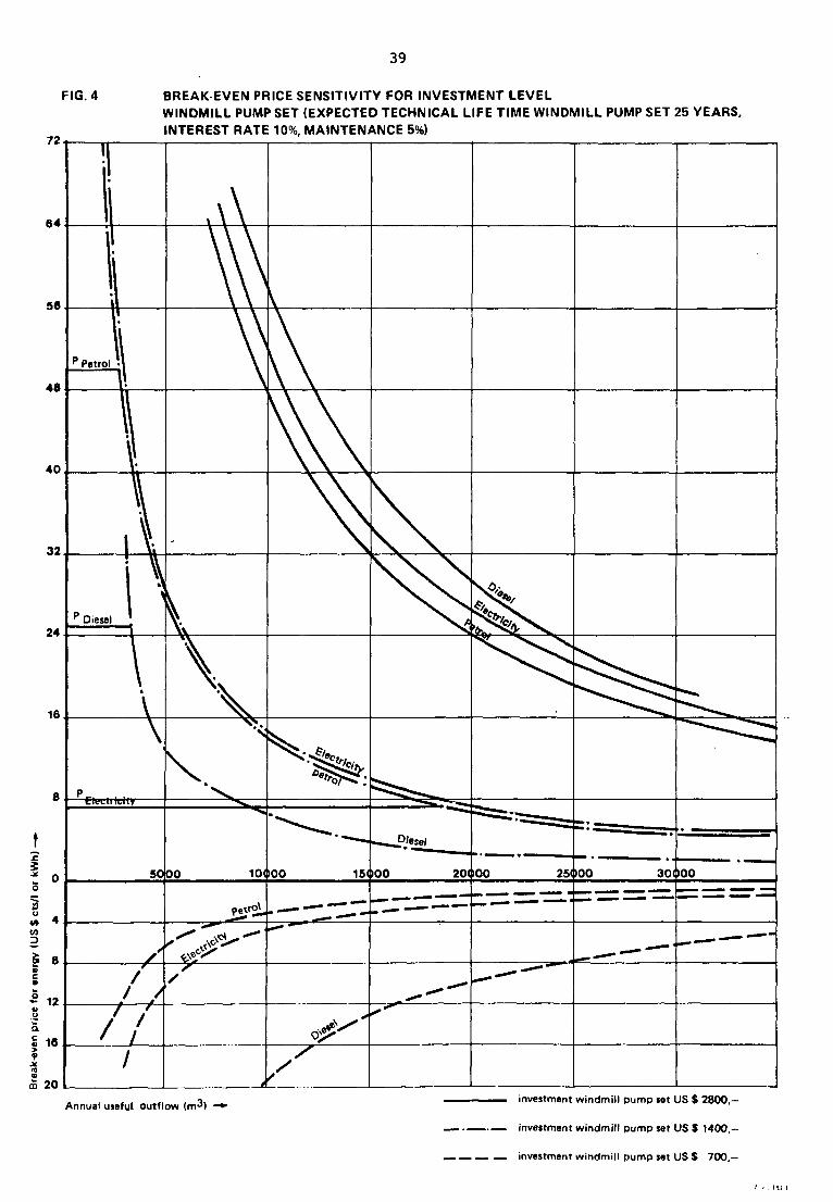
39
FIG. 4 BREAK-EVEN PRICE SENSITIVITY FOR INVESTMENT LEVEL WINDMILL PUMP SET (EXPECTED TECHNICAL LIFE TIME WINDMILL PUMP SET 25 YEARS, INTEREST RATE 10%, MAINTENANCE 5%)
Annual useful outflow (m3) -* • investment windmill pump set US $ 2800,
investment windmill pump set US $ 1400,-
_ _ _ _ _ _ investment windmill pump set US $ 700,-
40
Figure 4 shows negative break-even curves in case the investment of the windmill pump set drops to a level of US$ 700. This means that this windmill pump set is always preferable to its conventional engine driven alternatives. This is caused by the fact that for the US$ 700 windmill pump set the sum of the fixed annual costs (= annuity) and the variable costs of operation and maintenance 5% of the investment is less than the sum of the same items for the conventional engine driven pump sets. Even if the fuel price drops to zero the windmill pump set remains more attractive from an economic point of view. The negative break-even price for fuel indicates that the fixed costs advantage of the windmills is a bonus on top of the fuel savings.
It is noted that the assumed life time of the cheaper windmill in this comparison is maintained at 25 years. This may be considered too optimistic and therefore the influence of shorter technical life times of the windmill pump set is analysed in paragraph 3.8.3.
3.8.3. sensitivity to variation of technical life time of the
windmill pump sets
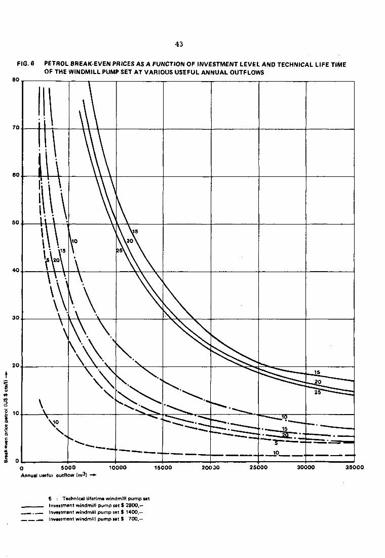
A relation is assumed to exist between the investment level and the life time of a windmill pump set. The construction of the 2800 dollar windmill pump set of the base situation may warrant a 25 years life time, while a 700 dollar windmill may last considerably snorter. Break-even prices are calculated for the three investment levels at various life times in Table 3.16. The influence of life time variation on the economic attractiveness of windmill pump set by means of a break-even price analysis at the running prices for fuel in The Netherlands is clearly shown by the thick line "stair case" in Table 3.16. Not all combinations of investment level and life time are relevant. A selection of realistic combinations is presented in figures 5, 6 and 7, assuming a positive relation between the investment level and life time of the windmill pump set. It follows from these figures that operation of the cheaper windmills remains favourable, even when considering relatively short technical life times.
3.8.4. Sensitivity to variation of maintenance costs
For the base situation maintenance and operation costs (excluding fuel costs) were estimated at 5% of the required investment. The influence of increasing the maintenance of the windmill pump set to 10% and more of the investment while keeping the maintenance costs of the conventional engine driven pump sets at the same level is shown in table 3.17. It follows from this table that the windmill pump sets of US $ 1400 and US $ 700 constitute interesting alternatives even with high levels of operation and maintenance costs. In case of the 700 dollar windmill pump set quadrupling of maintenance costs may be allowed, provided that by doing so a life time of 25 years can be attained.

Table 3.16 Influence of investment level and technical lifetime of the windmill pump set on the break - even prices for energy
(interest rate 10%).
Annual
useful out f low
(m3 )
2.000
5.000
10.000
15.000
20.000
25.000
30.000
35.000
Diesel (US$c ts / l )
investment windmil l pump set
US $ 2800
lifetime
5
788
315
158
105
79
63
53
45
10
461
184
92
61
45
37
31
25
15
362
145
72
48
35
29
24
21
20
316
127
63
42
32
25
21
18
25
292
117
58
39
29
23
19
17
U S $ 1400
lifetime
5
282
113
56
38
28
23
19
16
10
118
47
24
16
12
9
8
7
15
69
28
14
9
7
6
5
4
20
40
18
9
6
5
4
3
3
US $ 700
lifetime
5
29
12
6
4
3
2
2
2
10
neg
neg
neg
neg
neg
neg
neg
neg
15
neg
neg
neg
neg
neg
neg
neg
neg
20
neg
neg
neg
neg
neg
neg
neg
neg
Petrol (US $ Cts/I)
investment windmil l pump set
US $ 2800
lifetime
5
561
224
112
75
56
45
37
32
10
348
139
70
46
•35
28
23
20
15
284
113
57
38
28
23
19
16
20
254
101
51
34
25
20
17
15
25
238
95
48
32
24
19
16
14
US $ 1400
lifetime
5
231
92
46
31
23
18
15
13
10
125
50
25
17
12
10
8
7
15
92
37
18
12
9
7
6
5
20
77
31
15
10
8
6
5
4
US $ 700
lifetime
5
66
26
13
9
7
5
4
4
10
13
5
3
2
1
1
1
1
15
neg
neg
neg
neg
neg
neg
neg
neg
20
neg
neg
neg
neg
neg
neg
neg
neg
Electricity (US $ Cts/KWh)
investment windmil l pump set
US $ 2800
lifetime
5
630
252
126
84
63
50
42
36
10
388
155
78
52
39
31
26
22
15
315
126
63
42
32
25
21
18
20
281
113
56
38
28
23
19
16
25
264
105
53
35
26
21
18
15
USS 1400
lifetime
5
256
102
51
34
25
20
17
14
10
135
54
27
18
14
11
9
8
15
99
39
20
13
10
8
7
6
20
82
35
16
11
8
7
5
5
US $ 700
lifetime
5
69
28
14
9
7
5
5
4
10
9
3
2
1
1
1
1
1
15
neg
neg
neg
neg
neg
neg
neg
neg
20
neg
neg
neg
neg
neg
neg
neg
neg
1. Negative break-even prices indicate that the windmill pump set is always preferable to the other energy sources. 2. The "staircase" line indicates the break-even volumes at prevailing energy prices (1978). 3. Lifetime refering to technical lifetime of windmill pump set.

42
FIG. 5
80
DIESEL BREAK-EVEN PRICES AS A FUNCTION OF INVESTMENT LEVEL AND TECHNICAL LIFE TIME OF THE WINDMILL PUMP SET AT VARIOUS USEFUL ANNUAL OUTFLOWS
0 5000 annual Useful outflow (m^) .
10000 15000 20000 ?5000 30000 35000
5 Technical lifetime windmill pump tat Investment windmill pump set $ 2800,-Investment windmill pump set $ 1400,-
. __ Investment windmill pump set $ 700,—
43
FIG. 6 PETROL BREAK-EVEN PRICES AS A FUNCTION OF INVESTMENT LEVEL AND TECHNICAL LIFE TIME OF THE WINDMILL PUMP SET AT VARIOUS USEFUL ANNUAL OUTFLOWS
80.
0 5000 Annual useful outflow (m3)
10000 15000 20000 25000 30000 35000
6 : Technical lifetime windmill pump set Investment windmill pump set $ 2800,—
___ . _ _ Investment wlndmUl pump set $ 1400,— _ _ _ _ _ Investment windmill pump set $ 700,—

44 F I& 7 ELECTRICITY BREAK-EVEN PRICES AS A FUNCTION OF INVESTMENT LEVEL AND
TECHNICAL LIFE TIME OF THE WINDMILL PUMP SET AT VARIOUS USEFUL ANNUAL OUTFLOWS
5000 Annual useful outflow (m^) •
10000 15000 20000 25000 30000 35000
\
5 : Technical lifetime windmill pump set i Investment windmill pump set $ 2800,-
Investment windmill pump set $ 1400,-— — Investment windmill pump set $ 700,-
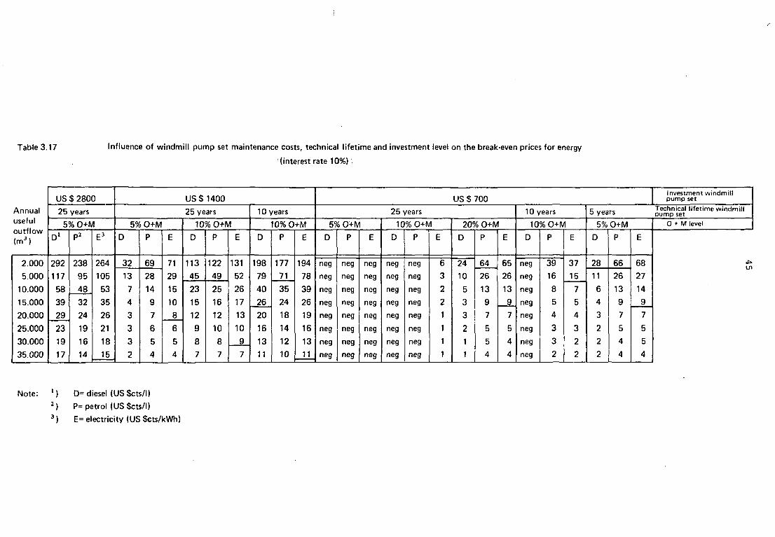
Table 3.17 Influence of windmill pump set maintenance costs, technical lifetime and investment level on the break-even prices for energy
(interest rate 10%).
Annual
useful
out f low (m3)
2.000
5.000
10.000
15.000
20.000
25.000
30.000
35.000
US $ 2800
25 years
5% O+M
D1
292
117
58
39
29
23
19
17
P2
238
95
48
32
24
19
16
14
E3
264
105
53
35
26
21
18
15
U S $ 1 4 0 0
25 years
5% O+M
D
32
13
7
4
3
3
3
2
P
69
28
14
9
7
6
5
4
E
71
29
15
10
8
6
5
4
10% O+M
D
113
45
23
15
12
9
8
7
P
122
49
25
16
12
10
8
7
E
131
52
26
17
13
10
9
7
10 years
10% O+M
D
198
79
40
26
20
16
13
11
P
177
71
35
24
18
14
12
10
E
194
78
39
26
19
16
13
11
US $ 700
25 years
5% O+M
D
neg
neg
neg
neg
neg
neg
neg
neg
P
neg
neg
neg
neg
neg
neg
neg
neg
E
neg
neg
neg
neg
neg
neg
neg
neg
10% O+M
D
neg
neg
neg
neg
neg
neg
neg
neg
P
neg
neg
neg
neg
neg
neg
neg
neg
E
6
3
2
2
1
1
1
1
20% O+M
D
24
10
5
3
3
2
1
1
P
64
26
13
9
7
5
5
4
E
65
26
13
9
7
5
4
4
10 years
10% O+M
D
neg
neg
neg
neg
neg
neg
neg
neg
P
39
16
8
5
4
3
3
2
E
37
15
7
5
4
3
2
2
Investment windmil l pump set
c . , „ _ r c Technical l i fet ime windmil l 3 yeo'S pump set
5% O+M
D
28
11
6
4
3
2
2
2
P
66
26
13
9
7
5
4
4
E
68
27
14
9
7
5
5
4
O + M level
•c*
Note: ' ) D=diesel (US$cts/l) ^) P= petrol (US $cts/l) 3) E= electricity (US $cts/kWh)

46
Introducing the energy prices in figures 8, 9 and 10 results in the corresponding annual useful outflows required to break-even.
For the energy prices as prevailing in The Netherlands the results are shown in table 3.18.
Table 3.18. Break-even water volumes as a function of investment and maintenance costs
Windmill pump set
US $ 2800 US $ 1400 US $ 700 US $ cts/liter 0 + M = 5% 0 + M = 10% 0 + M = 20% US $ cts/kWh (25 years) (25 years) (25 years)
Petrol 48 9,900 5,500 2,500 Diesel 25 23,200 8,900 1,700 Electricity 7.5 69,900 > 35,000 20,500
In 4 out of the 9 combinations the use of windmill pump sets (annual water demand: 9,502 m3) is profitable. In case all the potential water of the 2.2 m windmill can be applied (e.g. for the irrigation of 3 crops/year) the desirability of installing windmills increases to 5 out of 9 combinations.
Finally, if the potential water production of a 3 meter windmill could really be used (42,700 m3/annum) the windmill would be preferable to all alternatives.

47
FIG. 8 DIESEL BREAKEVEN PRICES AS A FUNCTION OF OPERATION AND MAINTENANCE COSTS OF THE WINDMILL PUMP SET
\ ?
X4-N ^ ,
^
^ - 2 2 * 25 „
Xo
>2
/̂
c
5000 Annual utaful outflow (m^) •
10000 15000 20000 25000 30000 35000

48
FIG. 9 PETROL BREAK EVEN PRICES AS A FUNCTION OF OPERATION AND MAINTENANCE COSTS OF THE WINDMILL PUMP SET
5000 Annual useful outflow (m3) •
O000 15000 20000 25000 30000 35000
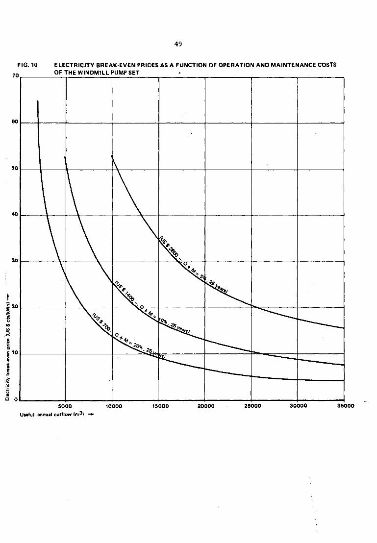
49
FIG. 10 ELECTRICITY BREAK-EVEN PRICES AS A FUNCTION OF OPERATION AND MAINTENANCE COSTS OF THE WINDMILL PUMP SET
nn
5 0
40
rv>
?0
m
0
I 1
> ,
^
x̂
K*/
<&«, ^ 5 ^ /
5000
UMful annual outflow (m3)
10000 15000 20000 25000 30000 35000

50
3.8.5. sensitivity to variation of interest rate
The economic analysis took into account an interest rate of 10% per annum in order to calculate the cost of capital. It may be considered that this interest rate is too high as a government might decide to provide credit on soft terms, for instance 6% per annum. It is also possible that no credit is available at 10% interest and that a farmer who wants to install a windmill will have to pay a higher interest rate, for instance 14%. The influence of a variation of the interest rate on the break-even prices for energy is analysed in table 3.19.
7i'able 3.19. Influence of the interest rate on the break-even prices for energy
Useful annuel 1 outflow (m3)
2000 5000
IOOOIO 15000 20000 25000 300DO 35000
Diesel (US $ xts/1)
interest
6
229 92 46 31 23 18 15 13
10
292 117 58 39 29 23 19 17
rate
14
363 145 73 48 36 29 24 21
Break-even
Petrol (US
price
$ cts/1)
interest
6
182 73 36 24 18 15 12 10
10
238 95 48 32 24 19 16 14
rate
14
303 121 60 40 30 24 20 17
Elect (US $
rici ty cts/kWh)
interest
6
202 81 41 27 20 16 14 12
10
264 105 53 35 26 21 18 15
rate
14
332 133 66 44 33 27 22 19
Note: all pump sets are defined as in the base situation
It follows from this table that variation of the interest rate has a relatively small influence on the feasibility of the windmill pump set. This is due to the fact that the variation of the interest rate was taken into account for the investment in the windmill as well as for the alternative sources of power. The influence of interest variation amounts to some 25% (plus or minus) as compared to the base situation. See also figure 11.

51
FIG. 11 BREAK-EVEN PRICES OF ENERGY AS A FUNCTION OF INTEREST RATE
e
\
0 Interest ratt •
6% 10% 14%
Outflow : 10000rr)3 Outflow : 35000 m3

52
Annuity factors to convert an including interest
6% lifetime in years
1 2 3 4 5 6 7 8 9 10
15 20 25 30 40 50
1.0600 0.5454 0.3741 0.2886
: 0.2374 0.2034 0.1791 0.1610 0.1470 0.1359
0.1030 0.0872 0.0782 0.0726 0.0665 0.0634
stment into an annual equivalent
8%' 10% 12%
1.0800 0.5608 0.3880 0.3019 0.2505 0.2163 0.1921 0.1740 0.1601 0.1490
0.1168 0.1019 0.0937 0.0888 0.0839 0.Q8L7
1.1000 0.5762 0.4021 0.3155 0.2638 0.2296 0.2054 0.1874 0.1736 0.1627
0.1315 0.1175 0.1102 0'l061 0.1023
•• 0.1009 J
1.1200 0.5917 0.4163 0.3292 0.2774 0.2432 0.2191 0.2013 0.1877 0.1770
0.1468 0.1339 0.1275 0.1241 0.1213 0.-1204

SWD 77-2: Cost comparison of windmill and engine pumps
Errata:
gage
3 Add: 3.8.6. Annuity factors (page 52)
8 line 7: change "a" into "or" and "alectricity" into "electricity",
line 11: change "exampte" into "example".
10. Add: (at the end of the note) over"a head of 13 m.
16. Change the formula into.-
P = h p V3 Q D 2 C nt % (W)
V=z
ih p.v3.n.D2.c .nv.n .w, (wh) V=a 4 P 't 'p d
32 Add: (beside figure) "scale"
33 Add: (at the top of the page) "3.8.6.".