Alireza Mousavi

Brunel University

1

» Computers in Control Systems

» Digital Control

» The z-Transform

» Discrete Time Systems

2

» autopilots for aeroplanes

» satellite altitude control

» industrial and process control

» Robotics and automation

» navigational systems and radar

» energy management and control in buildings and manufacturing

Advantages of computer control are:

» inherent reliability.

» ability to control many loops simultaneously.

» flexibility of control (i.e. control algorithm can be easily modified).

» increasing cost effectiveness of implementation.

» “intelligent” or “smart” control.

3

» real-time computer control first proposed in 1950 [Brown & Campbell, Mechanical Eng., 72: 124 (1950)]

» 1954 Digitrac digital computer

» closed-loop control: Texaco oil refinery, 15 March 1959.

» supervisory control: steady state optimizations to determine set points

» direct digital control: ICI plant at Fleetwood, UK, using Ferranti Argus 200

- provision for 120 control loops, 256 measurements

» 1974 microprocessor introduced

- distributed computer control systems

- microcontrollers (8051, 6811, PIC etc.)

4

Typical Digital Control System Or If digital control is used, it cannot be analysed as if it were a continuous control loop.

5

digital controller

actuator Processoutputset

point

measurement

+

-

digital controller

actuator Processoutputdigital set

point

measurement

However time and/or the value of the signal may be quantized.

6

t

(a) continuous time analog signal

y (t )

y (t )

t(b) continuous time quantized signal

y kT

t(c) sampled data signal

A discrete-time signal is one defined only at discrete instants of time (c & d).

» Normally assume

If the amplitude can assume a continuous range of values it is termed a sampled-data signal.

7

y * kT

t(d) digital signal

y * kT y kT k 0,1, 2, 3,

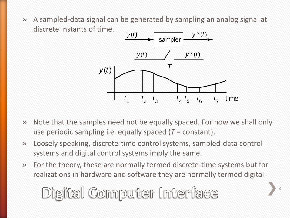
» A sampled-data signal can be generated by sampling an analog signal at discrete instants of time.

» Note that the samples need not be equally spaced. For now we shall only use periodic sampling i.e. equally spaced (T = constant).

» Loosely speaking, discrete-time control systems, sampled-data control systems and digital control systems imply the same.

» For the theory, these are normally termed discrete-time systems but for realizations in hardware and software they are normally termed digital.

8

y t y * t

y t y * t sampler

T

)

time

y (t )

t1

t2

t3

t4

t5

t6

t7

» Now consider the digital controller in more detail:

» Note: other parts of the loop may be discontinuous with respect to time - e.g. digital measuring device.

9

A/D converter

digital processor

D/A converter

Hold circuit

digital controller

continuous analog

discrete analog

discrete digital

continuous analog

discrete analog

discrete digital

e(t ) u (t )T

continuous controller

actuator Processoutputset

point

measurement

+

-

Thold

» Analog measurements and reference signals need to be sampled before digital processing in controllers

» Digital processing can be used for signal conditioning (DSP chips can function as Digital Controllers)

» Note that analog signals need to be preconditioned using analog circuitry before digitising to reduce:

˃ the problem of aliasing distortion (aliasing distortion: high frequency components above half the sampling frequency appearing as low frequency components. Happens when data are sampled from an analog (continuous) signal

˃ leakage (error due to signal truncation)

˃ noise reduction

10

The drive system of a plant normally takes an analog signal

Therefore the digital output from the controller has to be converted to analog

» Analog to digital converter (ADC, A/D)

- simultaneous A/D

- closed loop A/D (counter, successive approximation)

» Digital to analog converter (DAC)

» Hold devices: are analog devices that sample the voltage of a continuously varying analog signal and holds its value at a constant level for a specified minimum period of time (e.g. analog memory devices). - used in analog-to-digital converters to eliminate variations in input signal that can corrupt the conversion process.

» Digital Actuator: for example a stepper motor which responds with incremental motion steps when driven by pulse signals. A two position (position)solenoid (binary state).

11

» Digital control of flow can be achieved using digital control valve

12

spring-and-diaphragm actuator and FIELDVUE Digital Valve Controller Source Rotary Fischer)

A typical valve would have a number of Orifices each proportioned to the value Of binary word i.e. 20, 21, …

Digital Control Advantages:

1. Less susceptible to noise (presentable as discrete units)

2. Lends itself better to hardware software interfaces (fast-reliable)

3. Highly Programmable

4. Data can become compact (in case of large scale data handling)

5. Fast data transmission over long distances without excessive dynamic

delays compared to analog systems

6. Low operational voltage and cost effectiveness.

13

» We need to sample signals in computer control systems.

Nyquest-Shanon Sampling Theorem:

If a signal 𝑦(𝑡) (time signal) has no frequencies higher than its bandlimit 𝜔𝑐 and the sampling frequency to be 𝜔𝑠 ≥ 2𝜔𝑐 then the continuous signal 𝑦(𝑡) can be completely characterised by its sampled discrete signal 𝑦∗ 𝑡 .

Or: The Nyquest sampling criterion requires that the sampling rate for signal to be at least twice the highest frequency of interest.

Nyquest frequency 𝜔𝑁 = 1/2𝜔𝑠 of a discrete signal

14

Sampling of a pure sinusoid signal with frequency of 𝜔

𝑠𝑎𝑚𝑝𝑙𝑖𝑛𝑔 𝑖𝑛𝑡𝑒𝑟𝑣𝑎𝑙 𝑇 =2𝜋

𝜔 in other words 𝜔𝑠 = 𝜔

𝑠𝑎𝑚𝑝𝑙𝑖𝑛𝑔 𝑖𝑛𝑡𝑒𝑟𝑣𝑎𝑙 𝜋

𝜔< 𝑇 <

2𝜋

𝜔 in other words 𝜔 < 𝜔𝑠 < 2𝜔

15

t

y

y sint

0 𝜋

2 𝜋 3𝜋

2

2𝜋

t

y

y sint

𝑠𝑎𝑚𝑝𝑙𝑖𝑛𝑔 𝑖𝑛𝑡𝑒𝑟𝑣𝑎𝑙 𝑇 =𝜋

𝜔 in other words 𝜔𝑠 = 2𝜔

𝑠𝑎𝑚𝑝𝑙𝑖𝑛𝑔 𝑖𝑛𝑡𝑒𝑟𝑣𝑎𝑙 𝑇 <𝜋

𝜔 in other words 𝜔𝑠 > 2𝜔

16

t

y

y sint

t

y

y sint

» The functionality of a digital controller is similar to that of an analog one,

the only thing is that the I/O is in digital form.

» The control rules can be expressed by a set of differential equations.

» The differential equations relate the discrete outputs to the discrete

inputs of the controller.

» The challenge is to formulate the correct form of the difference equation

that could produce the required control signal.

» A digital controller can be defined as a number of discrete transfer

functions. Then those transfer functions can be turned into difference

equations.

17

» The discrete transfer functions depends on the sampling period 𝑇 to

convert analog signals into discrete data.

» The objective of a digital controller is to develop a deference equation

that represent the analog compensator, z-transform is used.

» When 𝑇 → 0 the digital control action approaches analog i.e. higher

frequency of sampling increases accuracy and lessens aliasing errors.

» Obviously faster rates of sampling imposes computational and

communication load on the computer system.

18

An infinite sequence of data:

𝑦𝑘 = {…𝑦−𝑘 , 𝑦−𝑘+1, … , 𝑦0, 𝑦1, … , 𝑦𝑘 , 𝑦𝑘+1, … }

Can be represented by a polynomial function of complex variable z:

∴ 𝑌 𝑧 = 𝑦𝑘𝑧−𝑘∞

𝑘=−∞ bilateral z-transform

𝑧 = 𝐴𝑒𝑗𝜑 = 𝐴(𝑐𝑜𝑠𝜑 + 𝑗𝑠𝑖𝑛𝜑)

Or Unilateral (single sided) z-transform: 𝑌 𝑧 = 𝑦(𝑘𝑇)𝑧−𝑘∞𝑘=0

as 𝑧 = 𝑒𝑠𝑡

multiplication by z is equivalent to a pure time advance of T seconds (i.e. 1 sample).

Or multiplication by 𝑧−1 is equivalent to a pure time delay of T seconds (i.e. 1 sample).

19

magnitude phase

Example 1. A unit step function:

𝑦 𝑡 = 1 𝑓𝑜𝑟 𝑡 ≥ 0

= 0 𝑓𝑜𝑟 𝑡 < 0 sampling period of T and the corresponding data sequence

to be 𝑦𝑘 = {0,0, … , 0,0,1,1, … , 1,1, … }

Find the z-transform of this sequence:

𝑌 𝑧 = 𝑧−𝑘 =1

1−𝑧−1=

𝑧

1−𝑧∞0

Example 2. find the z-transform of 𝑒−𝑎𝑡 , 𝑧{𝑒−𝑎𝑡}

𝑦 𝑡 = 𝑒−𝑎𝑡 ⇒ 𝑦 𝑘𝑇 = 𝑒−𝑎𝑘𝑇

∴ 𝑌 𝑧 = 𝑒𝑎𝑘𝑇𝑧−𝑘 = (𝑒−𝑎𝑇𝑧−1)𝑘= 1 + 𝑒−𝑎𝑇𝑧−1 + 𝑒−2𝑎𝑇𝑧−2 +⋯∞𝑘=0

∞𝑘=0

=1

1 − 𝑒−𝑎𝑇𝑧−1=

𝑧

𝑧 − 𝑒−𝑧𝑇

20

» Difference equations are discrete-time models.

» The Discrete-time model can be expressed by the nth order linear

difference equation:

𝑎0𝑦𝑘 + 𝑎1𝑦𝑘−1 +⋯+ 𝑎𝑛𝑦𝑘−𝑛 = 𝑏0𝑦𝑘 + 𝑏1𝑦𝑘−1 +⋯+ 𝑏𝑚𝑦𝑘−𝑚

» Provided that the 𝑢𝑘 is known the {𝑦𝑘} can be computed starting with

the first n values.

» The initial n values can be considered as the IC.

» 𝑎𝑖 and 𝑏𝑖 depend on sampling period.

21

Discrete-Time Model

{𝑢𝑘} Input seq.

{𝑦𝑘} output seq.

𝑍 𝑥𝑡 = 𝑋(𝑧)

Linearity :

Time Shift:

Final Value Theorem:

𝑍 𝑌 𝑠 = 𝑓 𝑒𝑇𝑠 𝑋 𝑠 = 𝑌 𝑧 = 𝑓 𝑧 𝑋(𝑧)

22

Z ay1 t by2 t aY1 z bY2 z

Z y t kT z kY z

limk

y kT limz1

1 z 1 Y z

Delay of k sampling period

In a series expansion the definition of Y(z) can be expressed as:

The expanded form of Y(z) the coefficients of the equation represent the

y(kT).

Example: Find y(kT) when

» Simplify using partial fraction, then use standard transforms.

» Note: many standard transforms have a zero at z=0

» Better to expand 𝑌(𝑧)

𝑧 and later multiply both sides of the equation by z.

» For no zeros at z = 0, use time-shift property

i.e. expand Y(z) as usual

then let 𝑌1 𝑧 = 𝑧(𝑌𝑧) and find 𝑦1(𝑘𝑇)

and then 𝑦 𝑘𝑇 = 𝑦1((𝑘 − 1)𝑇)

23

Y z y 0 y T z 1 y 2T z 2

Y z 0.3z

z 1 z 0.7

24

Y z 0.3z

z 1 z 0.7 𝑦 𝑘𝑇 =?

Y z

z

0.3

z 1 z 0.7

1

z 1

1

z 0.7

Y z z

z 1

z

z 0.7∴

y kT 10.7k , k 0,1, 2, 3,∴

» For a continuous-time system:

» If the input is sampled

» Now introduce a fictitious sampler on the output. It can be shown that:

∴

is defined as the pulse or z-transfer function of the system.

25

G(s)U(s) Y(s)

Y s G s U s or G s Y s

U s

G(s)U(s) Y(s)U*(s)

Y*(s)T

T (synchronised)

Y s G s U * s

Y * s G s U * s * G * s U * s

Y z G z U z

G z g kT z k

k 0

system impulse response sequence.

» Systems with samplers in cascade:

(assume all samplers are synchronised)

From the previous result:

And ∴

Overall z-transform function:

26

U(s) Y(s)U*(s)

Y*(s)T

T

E(s) E*(s)

TG1 s( ) G2 s( )

E z G1 z U z

Y z G2 z E z

Y z G1 z G2 z U z

G z G1 z G2 z

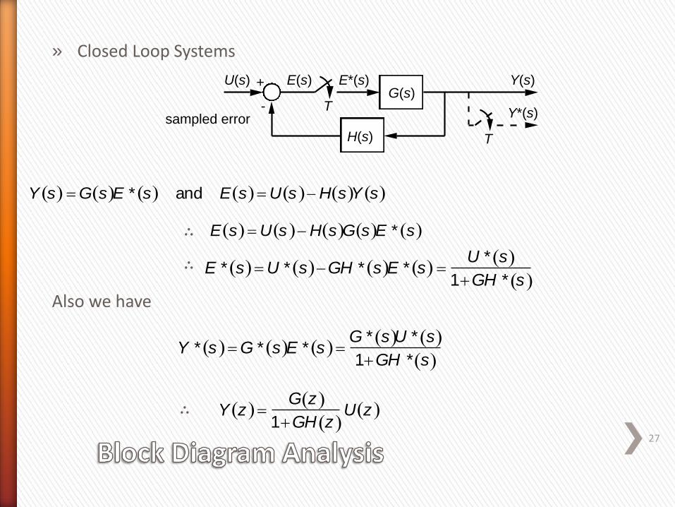
» Closed Loop Systems

∴

∴

Also we have

∴

27

U(s) Y(s)

H(s)

Y*(s)

T

E(s) E*(s)

TG(s)

sampled error

+

-

Y s G s E * s and E s U s H s Y s

E s U s H s G s E * s

E * s U * s GH * s E * s U * s

1GH * s

Y * s G * s E * s G * s U * s

1GH * s

Y z G z

1GH z U z

» The equation demonstrating the mapping between complex z-plane and

complex s-plane can be represented as:

𝑧 = 𝑒𝑇𝑠 (a)

The nature of this mapping.

Imagine a simple oscillator with undamped natural frequency 𝜔𝑛 and

damped natural frequency 𝜔𝑑 and damping ratio of ζ.

The complex poles (s-plane):

𝑠 = −ζ𝜔𝑛 ± 𝑗𝜔𝑑 (b)

28

jω

σ

Pole

Pole

𝜔𝑑

−𝜔𝑑

𝜔𝑛

𝜔𝑛

−ζ𝜔𝑛

𝜑

ζ=cos𝜑

Complex conjugate poles on the s-plane

From equations (a) and (b)

∴ 𝑧 = 𝑒𝑇(−ζ𝜔𝑛±𝑗𝜔𝑑) (c)

The magnitude of these two poles on the z-plane:

𝑧 = 𝑒−(𝑇ζ𝜔𝑛) (d)

Phase angle: ⦟𝑧 = ±𝑇𝜔𝑑

29

Three conditions:

1. Constant ζ𝝎𝒏 lines: based on equation (d), when ζ𝜔𝑛 is a constant.

Then 𝑧 is constant. Therefore ζ𝜔𝑛 constant lines on the s-plane (lines

parallel to imaginary vector of the s-plane. Maps to circles from the

origins of the z-plane.

30

𝑗𝜔

𝜎

𝐵− 𝐵+

0

0

𝐴 𝐵+

𝐵−

𝐴

−1 1

s- plane z- plane

𝑧 = 1 unit circle

Conditions continued:

2. Constant 𝝎𝒏 lines: from the angle phase equation (⦟𝑧 = ±𝑇𝜔𝑑), constant 𝜔𝑛(lines parallel to the real axis) map onto constant phase angles on the z-plane.

- Note that ⦟𝑧 = ±𝑇𝜔𝑑 refers to the many-to-one relationship.

𝑇𝜔𝑑 = 2𝜋𝑟 + 𝑐

- The fact that for any change in the integer value of r (a constant c) relates to a phase change by 2𝜋 in the z-plane which returns the line to the original position.

31

0

𝐵+

𝐵−

𝐴

𝑗𝜔

𝜎

𝐵−

𝐵+

0

𝐴

s- plane

z- plane 𝐴+

𝐴−

𝐴 𝐵

𝐴+

𝐵

𝑧 = 1 unit circle

Three conditions:

3. Constant ζ lines: constant ζ lines on the s-plane (straight lines through the origin) map into spiral lines on the z-plane

32

0

𝐴

𝑗𝜔

𝜎 0

𝐴

s- plane

z- plane

𝐴−

unit circle

𝐴−

stable

» With constant ζ𝜔𝑛 we note that the left hand side of the s-plane (representing stability) corresponds to the unit circle of the z-plane.

33

0 1

𝑗𝜔

𝜎 0

s- plane

z- plane

unit circle

−1

stable

» closed-loop stability is the most important consideration of control system design.

» For continuous-time systems, there are several methods to determine stability of a closed-loop system:

˃ Routh-Hurwitz criterion

˃ Nyquist criterion

˃ Bode plot

˃ root locus plot

(i.e. locations of the CL poles/eigenvalues in the s-plane)

» Only root locus can be applied directly in the z - plane.

34

» Recall the discrete signal :

Where

35

Y * s y kT e ksT

k 0

s s jns n 0, 1, 2,

Y * s jn s y kT e kT s jns

k 0

y kT e ksTe jknTs

k 0

Y * s

Y * s js\

is periodic with period

\

36

ZOH2

s2

Y(s)U(s)

G(z)

+

-

G z Z1 e sT

s

2

s 2

Z

2

s 3e sT 2

s3

Z2

s 3

z 1 Z

2

s 3

1 z 1 Z2

s 3

G z 1 z 1 ZG s

s

z 1

z

T 2z z 1 z 1

3let T 1

z 1

z 1 2

1G z 0

1z 1

z 1 2

z 1 2 z 1

z 1 2

0

z2 z 2 0 z 1 1 8

2

1

2 j

7

2

z 12

2 7

2 2

14

74 2 1

Generally

CLCE:

\

\

\

UNSTABLE

» Please refer to the annex of this lecture slides Lectures (no. 7b).

37