algorithms for pipe network analysis and their reliability
TRANSCRIPT

University of KentuckyUKnowledge
KWRRI Research Reports Kentucky Water Resources Research Institute
3-1981
Algorithms for Pipe Network Analysis and TheirReliabilityDigital Object Identifier: https://doi.org/10.13023/kwrri.rr.127
Don J. WoodUniversity of Kentucky
Click here to let us know how access to this document benefits you.
Follow this and additional works at: https://uknowledge.uky.edu/kwrri_reports
Part of the Theory and Algorithms Commons, and the Water Resource Management Commons
This Report is brought to you for free and open access by the Kentucky Water Resources Research Institute at UKnowledge. It has been accepted forinclusion in KWRRI Research Reports by an authorized administrator of UKnowledge. For more information, please [email protected].
Repository CitationWood, Don J., "Algorithms for Pipe Network Analysis and Their Reliability" (1981). KWRRI Research Reports. 76.https://uknowledge.uky.edu/kwrri_reports/76

Research Report No. 127
ALGORITHMS FOR PIPE NETWORK ANALYSIS AND THEIR RELIABILITY
By
Dr. Don J. Wood
Principal Investigator
Project Number: B-060-KY (Completion Report)
Agreement Number: 14-34-0001-9114 (FY 1979)
Period of Agreement: October 1978 - March 1981
University of Kentucky Water Resources Research Institute
Lexington, Kentucky
The work upon which this report is based was supported in part by funds provided by the Office of Water Research and Technology, United States Department of the Interior, Washington, D.C., as authorized by the Water Research and Development Act of 1978. Public Law 95-467.
March 1981


D IS CLAL111E R
Contents of this report do not necessarily reflect the views and
policies of the Office of Water Research and Technology, U.S. Department
of the Interior, Washington, D.c., nor does mention of trade names or
commercial products constitute their endorsement or recommendation for
use by the U.S. Government.


ABSTRACT
Algorithms for analyzing steady state flow conditions in pipe
networks are developed for general applications. The algorithms are
based on both loop equations expressed in terms of unknown flowrates and
node equations expressed in terms of unknown grades. Five methods,
which represent those in significant use today, are presented. An
example pipe network is analyzed to illustrate the application of the
various algorithms. The various assumptions required for the different
methods are presented and the methods are compared within a common
framework.
The reliabilities of these commonly employed algorithms for pipe
network analysis are investigated by analyzing a large number of pipe
networks using each of the algorithms. Numerous convergence and
reliability problems are documented. It is shown that two methods based
on loop equations have superior convergence characteristics. Methods
based on node equations are less reliable and these methods are often
unable to adequately handle low resistance lines. A discussion of
convergence criteria and solution reliability is presented for the
various algorithms. The results presented in this report will allow
engineers to accurately carry out pipe network analyses.
Descriptors: water distribution, piping systems, networks, convergence,
reliability
-2-

ACKNOWLEDGEMENTS
This work was supported by a grant from the Kentucky Water
Resources Research Institute under project A-076-KY and a grant from the
Office of Water Research and Technology, U,S, Dept, of Interior, under
project B-060-KY, Abid Rayes served as a graduate research assistant on
this project and provided much valuable assistance.
-3-

TABLE OF CONTENTS
Page
DISCLAIMER 2
ABSTRACT 2
ACKNOWLEDGEMENTS 3
LIST OF TABLES 6
LIST OF FIGURES 7
INTRODUCTION 8
ANALYSIS 12
Pipe Network Geometry 12
Basic Equations 12
Loop Equations 13
Node Equations 15
Algorithms for the Solution of Loop Equations 17
Single Path Adjustment (P) Method 18
Simultaneous Path Adjustment (SP) Method 19
Linear (L) Method 20
Algorithms for the Solution of Node Equations 21
Single Node Adjustment (N) Method 21
Simultaneous Node Adjustment (SN) Method 22
EXAMPLE CALCULATIONS 25
Algorithms Based on the Loop Equations 26
Single Path Adjustment Method 26
Simultaneous Path Adjustment Method 28
Linear Method 28
Algorithms Based on the Node Equations 29
Single Node Adjustment Method 30
Simultaneous Node Adjustment Method 30
Comparison of Final Results 31
COMMENTS ON METHODS 3 3
DATA BASE FOR STUDY 34
COMPUTER PROGRAMS FOR COMPARISONS 36
Convergence Criterion 37
Accuracy of Solutions 37
COMPARISON OF SOLUTIONS 39
-4-

DISCUSSION AND ADDITIONAL RESULTS
CONCLUSIONS
REFERENCES
NOTATION
APPENDIX
APPENDIX 1
APPENDIX 2
APPENDIX 3
APPENDIX 4
APPENDIX 5
Computer Programs
Single Path Adjustment Method
Simultaneous Path Adjustment Method
Linear Method
Single Node Adjustment Method
Simultaneous Node Adjustment Method
-5-
Page
41
46
49
52
54
59
66
74
81
89

Number
l
2
3
4.
5
6
7
8
9
10
11
12
13
14
15
16
17
18
19
20
21
LIST OF TABLES
Title
Pipe System Constants
Initial Values for Gi and Hi
Calculations for SP Method
Values of Qi, Gi and Hi for L Method
Calculations for SN Method
Comparison of Solutions for Example
Systems Under 100 Pipes
Systems Over 100 Pipes
Comparisons of Flowrates and Grades - 14 Pipe
System
Checks on Accuracy and Convergence - 14 Pipe
System
Summary of Failures - SP Method
Summary of Failures - P Method
Summary of Failures - SN Method
Summary of Failures - N Method
Results for Land SP Methods - Over 100 Pipes
Results for SP Method - Higher Accuracy
Results for Tank Flows - 79 Pipe System
Documentation of Convergence Problem - SN Method
Results for SN Method - More Trials - Higher
Accuracy
Results for N Method - Higher Accuracy
Results for N Method - More Trials
-6-

Number
l
2
3
4
5
6
LIST OF FIGURES
Title
Pump Notation for Node Equations
Example Pipe System
Initial Conditions for Example Calculations
Pipe and Node Numbering - SN Method
Pump Operation Characteristic Curve
Fourteen Pipe System
-7-
INTRODUCTION
Steady state analysis of pressure and flow in piping systems is a
problem of great importance in engineering. The basic hydraulics
equations describing the phenomena are non-linear algebraic equations
which can not be solved directly. These equations have been expressed
in two principal fashions. They have been written in term of the
unknown flowrates in the pipes herein referred to as loop equations.
Alternately, they have been expressed in terms of unknown grades at
junctions throughout the pipe system (node equations). Several
algorithms have been proposed for solving these equations and these
techniques are in wide use today.
In this report the principal algorithms are developed for
applications to piping systems of general configuration and systems
which contains pumps and other common hydraulic components. In most
situations the algorithms have been previously presented with
limitations on pipe system configurations and components which can be
considered. An example system is analyzed using each of the algorithms
to illustrate the required computational procedures. The efficiency and
reliability of these algorithms are examined by solving a large number
of actual pipe network problems with each algorithm and comparing the
results.
There is a considerable amount of published material dealing with
pipe network analysis, all of which can not be reviewed here. However,
an attempt will be made to cite some principal contributions of
historical interest. Hardy Cross authored the original and classic
paper (1). In that article, which considered only closed loop networks
with no pumps, a method for solving the loop equations based on
adjusting flowrates to balance the energy equations is described. This
method is very widely used today and is often referred to as the Hardy
Cross method. Although it is not as widely used, Hardy Cross described
a second method for solving the node equations by adjusting grades so
that the continuity equations are balanced. A number of subsequent
papers have appeared which further describe these methods or computer
-8-

programs utilizing these methods (2, 3, 4, 5, 6).
Because the adjustments are computed independently from each other,
convergence problems using the methods described by Hardy Cross were
frequently noted and procedures developed to improve convergence.
Martin and Peters (7) and Epp and Fowler (8) described a procedure to
simultaneously compute the flow adjustments for closed loop systems.
This procedure had much improved convergence characteristics and forms
the basis for more general applications (5, 9).
Both the methods just described for solving the loop equations
require an initial balanced set of flowrates and the convergence depends
to a degree on how close this initial set of flowrate is to the correct
solution. A third method, developed by this writer solves the entire
set of hydraulics equations simultaneously after linearizing the energy
equations. This procedure was first described for closed loop systems
(10) and has subsequently been modified for more general applications
(11, 12). A similar approach has been developed for the node equations
where all the equations are linearized and solved simultaneously, and
this method is described for closed loop systems by Shamir and Howard
(13). Additional references to this method have been published (14,
15).
The five methods just described are developed in detail in the next
section for general applications. No restrictions on network geometry
are required and pumps may be included anywhere in the network. Certain
special components such as check valves and pressure regulating valves
are not considered since these components require special treatment.
Each of these methods for pipe network analysis discussed in this
report require iterative computations whre the solution is improved
until a specified convergence criterion is met. If a sufficiently
stringent convergence criterion is met, the solutions normally will be
essentially identical for all five methods. In some cases, however, it
is not possible with certain algorithms to meet a specified convergence
criterion regardless of the number of trials completed. In other cases
a seemingly stringent convergence criterion may be met but the solution
is still in considerable error. Convergence difficulties such as these
have been previously noted and reported. In this report, results are
presented of a detailed study that documents convergence problems and
-9-

program efficiency.
obtained with the
This study was carried out by comparing solutions
various algorithms using an extensive data base
describing a variety of actual piping systems operating under widely
varying conditions ••
In the original paper by Hardy Cross he noted that "convergence was
slow and not very satisfactory" when employing the single node
adjustment method he developed (1). This was attributed to using
initial grade estimates which were not very good. Of the two methods
described by Hardy Cross, the method of balancing heads (single path
adjustment method) became the most widely taught and used method.
Convergence problems using this method were also recognized, however,
and several suggestions were made for improving convergence.
Investigators have advocated the use
multiply the flow adjustment factor
of an over-relaxation factor to
(16, 17). Hoag and Weinberg
suggested using a selective procedure for choosing paths as a means of
accelerating convergence (18). It appears that these and other
procedures suggested for improving convergence of the single path
adjustment method will improve it only in certain situations and will
not assure convergence.
Convergence problems are
methods developed for solving
largely unreported for the
the loop equations. These
improved
are the
simultaneous path adjustment and the linear methods which are included
in the current study. However, additional convergence problems have
been reported for methods based on the node equations since Hardy Cross
first alluded to such problems in his original paper. Dillingham (4)
stated that when the single node adjustment method is applied to a large
network it may not converge or may converge very slowly. He described
some procedures for improving convergence. Robinson and Rossum (6) who
developed a computer program based on the single node adjustment method
state that, "convergence is slow when a network contains short lengths
of large diameter mains and cnvergence is not assured if there are dead
end mains." They further state that "convergence may not occur if
check valves are present." The simultaneous node adjustment method
normally converges much more rapidly which lead Lemieux to state that
convergence was assured (14). However, it appears that this assessment
is optimistic and problems have been noted with this method.
-10-

Oscillations have been noted by Shamir and Howard (13) who also report
that there is a possibility that a solution can not be obtained. Liu
also stated "for poor initial input the method (simultaneous node
adjustment) may diverge from the true solution or converge slowly" (15).
Collins and Kennington presented some data which documented convergence
problems for a large network using this method. (19).
The reliability of the algorithm employed for pipe network analysis
if of great importance and the most single significant consideration.
Failure to obtain a solution is a great inconvenience and the failure to
recognize a poor solution may be even a greater problem because this may
lead to poor design or management of water distribution systems. The
purpose of this study is to document reliability problems which may
occur using the various popular algorithms so that the frequency and
severity of such problems will be known.
-11-

ANALYSIS
Pipe Network Geometry
Basic geometric considerations for a pipe network are summarized as
follows, A pipe network is comprised of a number of pipe sections which
are constant diameter sections which can contain pumps and fittings such
as bends and valves. The end points of the pipe sections are nodes
which are identified as either junction nodes or fixed grade nodes. A
junction node is a point where two or more pipe sections joins and is
also a point where flow can enter or leave the system, A fixed grade
node is a point where a constant grade is maintained such as a
connection to a storage tank or reservoir or to a constant pressure
region. In addition primary loops can be identified in a pipe network
and these include all closed pipe circuits within the network which have
no additional closed pipe circuits within them. When junction nodes,
fixed grade nodes, and primary loops are identified the following
relationship holds:
where
p = j + i + f - 1
p • number of pipes
j = number of junction nodes
£ = number of primary loops
f = number of fixed grade nodes
(l)
It turns out that this identity is directly related to the basic
hydraulics equations which describe steady state flow in the pipe
network,
Basic Equations
Pipe network equations for steady state analysis have been commonly
expressed in two ways. Equations which express mass continuity and
energy conservation in terms of the discharge in each pipe section have
been referred to as loop equations and this terminology will be followed
-12-

here, A second formulation which expresses mass continuity in terms of
grades at junction nodes produces a set of equations referred to as node
equations.
Loop Equations - Eq. l which defines the relationship between the
number of pipes, primary loops, junction nodes and fixed grade nodes
offers a basis for formulating a set of hydraulic equations to' describe
a pipe system. In terms of the unknown discharge in each pipe, a number
of mass continuity and energy conservation equations can be written
equaling the number of pipes in the system. For each junction node a
continuity relationship equating the flow into the junction (Qin) to the
flow out (Q ) is written as: out
(j equations) (2)
Here Q represents the external inflow or demand at the junction node, e
For each primary loop the energy conservation equation can be written
for pipe sections in the loop as follows:
where
l:h. = l:E L p
(t equations)
~=energy loss in each pipe (including minor loss)
E = energy put into the liquid by pumps p
(3)
If there are no pumps in the loop then the energy equation states that
the sum of the energy losses around the loop equals zero,
If there are f fixed grade nodes, f l independent energy
conservation equations can be written for paths of pipe sections between
any two fixed grade nodes as follows:
(f-1 equations) (4)
where 6E is the difference in total grade between the two fixed grade
nodes. Any connected path of pipes within the pipe system can be chosen
between these nodes. When identifying these f - l energy equations care
must be taken to avoid redundant paths, The best method to avoid this
-13-

difficulty is to either choose all parallel paths starting at a common
node (like A-B, A-C, A-D, etc) or to use a series arrangement where the
previous ending node for a path is the starting node for the next path
(like A-B, B-C, C-D, etc,). Either of these methods will results inf -
l equations with no redundancy.
As an additional generalization Equ. 3 can be considered to be a
special case of Equ. 4 where the difference in total grade (Ii E) is zero
for a path which forms a closed loop. Thus, the energy conservation
relationships for a pipe network are expressed by t + f - l energy
equations of the form given by Equ. 4. The continuity and energy
equations constitut a set of p simultaneous nonlinear algebraic
equations referred to as loop equations which describe steady state flow
conditions within a system of pipes. A steady state flow analysis based
on the loop equations requires the solution of this set of equations for
the flowrate in each line. To do this the terms in the energy equations
must be expressed as functions of the flowrate which is done as follows.
The energy loss in a pipe (1,.) is the sum of the line loss (1\p)
and the minor loss (1,.M). The line loss expressed in terms of the
flowrate is given by:
(5)
where ~ is a pipe line constant which is a function of line length,
diameter, and roughness, and n is an exponent. The values of~ and n
depend on the energy loss expression used for the analysis. Commonly
used expression for this include the Darcy-Weisbach, Hazen Williams and
Manning Equations.
The minor loss in a pipe section (1\M) includes losses at fittings,
valves, meters and other components which disturb the flow and is given
as
(6)
where ~ is the minor loss constant which is a function of the sum of
the minor loss coefficients for the fittings in the pipe section (EM)
-14-

and the pipe diameter and is given by
~ = EM/2gA2 (7)
where A is the cross-sectional pipe area,
Pumps are described several ways. In some cases a constant power
input is specified, In other cases a curve is fit to actual pump
operating data. A variety of functions have been suggested for the
curve chosen to fit the data and a common choice is a second order
polynominal. For all the applications involving pumps the relationship
between the pump energy, EP' and discharge, Q, can be specified by a
reasonably simple expression
E = P(Q) (8) p
Utilizing Equs, 5-8 the energy equations expressed in terms of the
flowrate are
(9)
The continuity equations (Equ, 2) and the energy equations (Equ. 9)
form the set of p simultaneous equations in terms of unknown flowraes
which are termed the loop equations. Since these are nonlinear
algebraic relationships no direct solution is possible. Three
algorithms for solving the loop equations are presented in this paper.
Node Equations - The analysis is carried out in terms of an unknown
total grade, H, at each junction node in the piping system. The basic
relationship used is the continuity relationship (Equ. 2)
The flowrate in a pipe section connecting nodes labeled a and b is
expressed in terms of the grade at junction node a, Ha' the grade at the
other end of the pipe section,!\, and the resistance of the pipe, Kab'
-15-

This is
1/n (10)
This expression assumes that the pipe section contains no pumps and a
head loss relationship is used of the form
(11)
where the term K is the loss coefficient for the pipe section and is a
function of pipe parameters and flow conditions and depends on the head
loss expression used and may include minor loss terms. The exponent n
also depends on the head loss expression used.
Combining Equs. 2 and 10 gives:
N + E
b=l
H - H a b
Kab
1 n
(j equations) (12)
This expresses continuity at junction node a where N pipes connect in
terms of the grade at a, H and the grades at adjacent nodes, H.. The a' --b
sign of the term in the summation depends on whether the flow is into or
out of junction node a. A total of j equations are written in this
manner.
The basic set of equations can be expanded to incorporate pumps.
For each pump junction nodes are identified at the suction and discharge
sides of the pump as shown in Figure l. Two additional equations can be
written in terms of the two additional unknown grades at the suction and
discharge sides of the pump and the adjacent grades.
Using the notation shown in Figure l, one equation utilizes flow
-16-

a
A 50psi
j1001j
EA •215.38f
b c
Figue I Pump Notation for Node Equations
200'6"
d
B
'J,1=10 ( globe valve)
C• 130 (all pipes)
O Junction node numbe~
D elevations
(> pipe numbers
Figure 2 Example Pipe Sys1em(lf.•.3048m,I in.=2.54cm,Jf31\1 •.028m31\1 ,l#"/in 2 =689.5N/m 2 ,I Hp•.746 KW)

continuity in the suction and discharge lines to give
(13)
A second equation relates the head change across the pump to the flow in
either the discharge-or suction line, For pumps operating at constant
power this relation in terms of the discharge line flow is
H - H = P( c b
Equations 12-14 represent the
equations which are expressed in terms
nodes and pump suction and discharge
(14)
full set of pipe network node
of the unknown grades at junction
grades at all pumps in the pipe
system, Like the loop equations, these are nonlinear algebraic
equations and no direct solution is possible,
Algorithms for the Solution of the Loop Equations
Three methods for the solution of the loop equations have been
developed and are in significant use today. Each of these use gradient
methods to handle the non-linear flowrate (Q) terms in the energy
equation (Equ, 9), The right side of Equ, 9 represents the grade
difference across a pipe section carrying a flowrate Q. This is
f(Q) = ~Qn + ~z - P(Q) (15)
The function and its gradient evaluated at an approximate value of the
flowrate, Qi' are used in all the algorithms presented for solving the
loop equations. The grade difference in a pipe section based on Q=Qi
is:
2 = K...Q. - P(Q.) --p ]. ]. (16)
-17-

and the gradient evaluated at Q
(17)
Q=Q. 1.
The terms Hi and Gi as defined above are referenced in the
following discussion of the algorithms for the loop equations and the
example calculations which illustrate the application of these
algorithms to pipe network problems.
Single Path Adjustment (P) Method. - This method of solution was
described by Hardy Cross (1) and is the oldest and most widely used
technique. The original method was, however, limited to closed loop
systems and · included only line losses. Herein the procedure is
generalized. The method of solution is summarized as follows:
1. Determine an initial set of flowrates which satisfy continuity
at each junction node.
2. Compute a flow adjustment factor for each path ( £ + f - 1) in
the pipe system which tends to satisfy the energy equation written for
that path. The application of this correction factor will not disturb
the continuity balance.
3. Using improved solutions for each trial repeat step 2 until the
average correction factor is within a specified limit.
The adjustment factor for a path is computed from equation 9 using
a gradient method for solving a nonlinear equation for a single unknown.
This method is based on the following approximation for the terms in
equation 9 which are functions of the flowrate Q.
:lf
:lQ LIQ
Q=Q. 1.
(18)
where Qi is an approximate value of the flowrate. Applying Equ. 18 to
the line loss, minor loss and pump energy terms in Equ. 9 and solving
-18-

for LIQ gives:
LIQ = LIE - EH.
l.
EG. l.
(19)
The E means that the contribution from each pipe in the path must be
included. The terms LIQ represents the flowrate adjustment factor which
must be applied to each pipe in the path. The numerous represents the
unbalance in the energy relationship due to the incorrect flowrates and
the procedure is developed to reduce this to a negligible quantity, A
trial with this method requires a flow adjustment to all paths in the
pipe network ( t loop and f - 1 paths between fixed energy nodes).
Simultaneous Path Adjustment (SP) Method. - In order to improve the
convergence characteristics a method of solution was devised which
simultaneously ad justs the flowrate in each path of pipes representing
an energy equation (2), This method can be summarized as follows.
1, Determine an initial set of flowrates which satisfy continuity
at each junction mode.
2, Simultaneously compute a flow adjustment factor for each path
which tends to satisfy the energy equations without disturbing the
continuity balance.
3. Using the improved solutions repeat step 2 until the average
flow adjustment factor is within a specified limit,
The simultaneous determination of the path flow adjustment factors
requires the simultaneous solution of t + f 1 equations. Each
equation accounts for the unbalance in the energy equation due to
incorrect values of flowrate. The equation includes the contribution
for a particular path as well as contributions from all other paths
which have pipes common to both paths. Gradient techniques are used to
formulate these equations. For path j, the head change required to
balance the energy equation is expressed in terms of the flow change in
path j (LIQj) and the flow changes in adjacent paths (6QK) and is given
as:
-19-

oH L\H = aQ L\Q.
J
Q=Q. 1.
+ aH aQ
(20)
This can be expressed in terms of Hi and Gi for 'the pipes in the path as
follows
(21)
Here rn. represents the algebraic sum of the head changes for all the l.
pipes in path j, (EGi)L\Qj represents the sum of all the gradients for
the same pipes times the flow change for that path and E (Gi L\QK)
represents the sum of the gradients for pipes common to paths j and K
times the flow change for path K, The last term is repeated for all
paths with pipes common to path j,
In this manner a set of simultaneous linear equations are formed in
terms of flow adjustment factors for each path representing an energy
equation, ~ese linear equations can be solved using standard
procedures and the solution provides an improved set of balanced
flowrates which can be used for another trial.
until a specified accuracy is attained.
Trials are repeated
Linear (L) Method. - This method is based on a simultaneous
solution of the basic hydraulics equations for the pipe system and has
been reported for closed loop systems (3) and general systems (4).
Since the energy equations for the paths are non-linear, these equations
are first linearized in terms of an approximate flowrate, Q., in each l.
pipe. This is done by taking the derivative of the variables in Equ. 9
with respect to the flowrate and evaluating them at Q = Q. using the 1.
following approximation
When this relationship is applied to the energy equation (Equ. 9)
the following linearized equation results:
EG.Q = E(G.Q. - H.) + L\E ]. 11 l.
(22)
The E refers to each pipe in the path. Equ, 23 is employed to
formulate i + f - l energy equations which combine with the j continuity
equations (equs. 2) to form a set of p simultaneous linear equations in
terms of the flowrate in each pipe.
-20-

The technique used to solve the system equations follows. Based on
an arbitrary initial value for the flow in each line the linearized
equations are solved using routing matrix procedures for solving linear
equations. This set of flowrates is used to linearize the equations and
a second solution is obtained. The procedure is repeated· until the
change in flowrates obtained in successive trials is insignificant.
Algorithms for the Solution of Node Equations
Two methods for solving the node equations are widely used and
these are described here.
Single Node Adjustment (N) Method - This method was also described
in the paper written by Hardy Cross (1). However, the method has never
been widely used as the single path adjustment method. It is,
nevertheless, in significant use today. The method is summarized as
follows:
1. Assume a reasonable grade for each junction node in the system.
This assumed grade does not have to satisfy any conditions. However,
the better the initial assumption the fewer the required trials.
2. Compute a grade adjustment factor for each junction node which
tends to satisfy flow continuity.
3; Repeat step 2 until the average correction factor for grades is
within a specified accuracy or some other specified convergence
criterion is satisfied.
The grade adjustment factor is the change in grade at a particular
node ( AH) which will results in satisfying continuity (Equ. 2)
considering the grades at the adjacent nodes as fixed. Again a gradient
approximation is used to compute the required grade change. This is:
f(H) = f(H.) + _l_i__ l. a H AH
H=H. l.
(25)
It is convenient to express the grade correction factor in terms of Q. l.
which is the flowrate based on the values of the grades at adjacent
-21-

nodes before adjustment. This gives the following factor for the grade
adjustment factor:
6.H = + EQ. - Q 1 e
E _! G.
1
(26)
where the E indicates the contribution from each pipe section connecting
the node and these are added algebraicly with inflow positive. The
numerator represents the unbalanced flowrate at the junction node.
The value of flowrate in a pipe section prior to adjustment, Qi is
computed based on the initial values of the grades at the ends of the
pipe section. For sections with minor loss components this calculation
is simplified if the loss coefficient for the pipe section is modified
to include the minor loss term as suggested previously.
flowrate is
Q = (6.H /K)l/n i i
The initial
(27)
where 6.Hi is the grade change across the pipe section based on the
initial values of grade. If pumps are included then Qi must be
determined from the expression
(28)
Equ. 28 is not difficult to solve but may require the employment of an
approximation procedure to solve this non-linear expression. A single
trial for this method requires the adjustment of the grade for each
junction node within the pipe system. The trials continue until the
specified convergence criterion is met.
Simultaneous Node Adjustment ( SN) Method. - This me tt,od is based on
a simultaneous solution of the basic pipe network node equations and
requires a linearization of these equations in terms of approximate
values of the grade(l3). Equ. 12 can be linearized with respect to the
-22-

grades if the flowrates are written in terms of some approximate or
initial values of the total grades, Hai and ~i, and the changes in
these grades. This uses the following to calculate the flowrate in pipe
section ab.
Q = Q +-1L tiH +!1-H- t,Hb i :lH a o (29)
When the flowrate is expressed by Equ. 10, this can be solved to give:
(30)
The initial value of flowrate, Qi, in computed based on the initial
values of the grades and is
1 (31) -n
where Kab is the loss coefficient for line ab including minor losses if
any.
Using Equ. 30, the continuity equation for each junction can be
written as a linear function of the variable and fixed grades of the
adjacent nodes and the variable grade of junction, a. This is:
N 1-n N 1-n v G. Q.
i: ].
~- H i: ].
b=l nKab a b=l nKab
N N Qi
NF 1-n Q + l: Q. + l: v - I\ i: Qi (32) e-
b=l1 b=l n b=l nKab
-23-

Here N refers to all adjacent nodes, N refers to all adjacent variable v
grade nodes and NF refers to all adjacent fixed grade nodes. The:!:: sign
depends on whether Qi is into or out of -junction a and is positive for
inflow.
Equ. 32 is written for each junction node in the system resulting
in a set of linear equations in terms of junction node grades. For each
pump in the system two additional equations are introduced which are
functions of the pump suction and discharge pressure. Equ. 13 is linear
and can be incorporated directly into the linearized equation set. Equ.
14 is non-linear but can be linearized using gradient methods and
results in the following linearized equation:
H ( l +'<) - ll - H .B = a c - -0 d . (33)
Here c,. and S depend on the relationship used to describe the pump, P(Q),
and are given by
a = P(Qi) + Qi p• (Qi) n
s P' (Qi)
nK Q':'-1 cd 1
The preceeding procedure produces a set of
linear equations (where n is the number of pumps). p
solved as follows: Starting with Qi' s based on
values for the junction node grades these linear
{34)
(35)
j + n simultaneous p
These equations are
any assumed set of
equations are solved
simultaneously for an improved set of junction node grades. These are
used to compute an improved set of Qi's and the procedure repeated until
subsequent calculations satisfy a stated convergence or accuracy
criterion.
-24-

EXAMPLE CALCULATIONS
The use of the five methods of analysis presented are best
illustrated by an example water distribution system which is analyzed by
each of the methods. The calculations are illustrated for one trial for
each method. Additional trials were carried out and the solutions are
compared after each method met a specified convergence criterion. The
system utilized is shown in Fig. 2. All the necessary data is presented
and numbers are assigned to the pipe sections and junction nodes.
English units are employed for this example and appropriate conversion
factors for SI units are noted on Fig. 2. This system includes one
component, a globe valve in pipe no. 7, which has a significant minor
loss coefficient. Other minor losses are neglected. A pump which
inputs a constant power into the system is included in pipe no. 2. The
useful horsepower (HP) u
for this pump is given. For this pump
representation Equ. 8 becomes
Ep = P(Q) = Z/Q (36)
where the pump constant Z = 550 HP /62 .4 = 44 .07 for this pump. The u
pump terms in the various solution procedures are
(37)
and (38)
For the example the Hazen Williams equation is employed for head
loss calculations. For this expression the pipe line contant is
4.73 L KP= Cl.852 D4.87 (39)
and n = 1 .852 where L is the length, D is the pipe diameter. The
roughness value C is defined in Fig. 2 as 130 for all the pipes. Table
1 summarizes values of pipe line, minor loss and pump constants for each
pipe in the example system.
-25-

Pipe No. KP \r z
l 3.36 0 0 2 18.18 0 44.1 3 73.78 0 0 4 76.24 0 0 5 2.69 0 0 6 24.23 0 0 7 122.97 64.44 0
Table 1 - Pipe System Constants
These are used for all of. the algorithms which are illustrated in the
following sections.
Algorithms Based on the Loop Equations
For the example systems the loop equations include four mass
continuity for the four junction nodes noted and three energy equations.
The energy equations include one for each of the two loops noted (t, E •
0) and one additional energy equation for pipes connecting the two fixed
grade nodes {ll.E • 25.38f). Two of the three methods discussed for
solving the loop equations require an initial set of balanced flowrates
and the values used for this example are shown in Fig. 3. Values for
the initial grade change, Hi' and the initial gradients, Gi' computed
using Equs. 16 and 17 using the initial flowrates are shown in Table 2.
Q. G. H. Pioe No. 1 1 1
1 2 11.24 12. 14 2 1.5 67. 14 9.13 3 .6 88.43 28.64 4 .4 64.68 13.97 5 .5 2.76 .75 6 . 1 6.31 .34 7 .4 155.88 32.84
Table 2 - Initial Values for G. and H. 1 1
Single Path Adjustment Method - A trial for this method involves
adjusting each of the three energy equations using Equ. 19. The
calculations for the first trial are shown in Table 3. Path AB is first
adjusted using pipes 1, 2, 3 and 4. Alternate pipes connecting AB could
have bee~ chosen. T~e computed flow adjustment of .178f3/s is applied
immediately to the pipes in path AB and subsequent calculations using
-26-

A
HA= 215.38f.
* -Grade - - Flowrate (in direction indicated)
200*
®
Figure 3 Initial Flowrates (inf3/s l and Grades (inf) for Example Calculations
B
Figure 4 Pipe and Node Numbering and Initial Pump Grades{*) for Simultaneous Node Method

these pipes will enploy the adjusted flowrate Qf, and values of G1 and
Hi based on these, The second adjustment shown for loop I is carried
out in the sense depicted in Fig. 3 and flows in that sense are taken as
positive. The sign for . the grade change, Hi, is the same as the
flowrate while all the gradient terms, Gi' have positive signs. Loop II
is then adjusted in the same fashion and this completes the first trial,
A second trial is carried out in the same manner using the most recently
determined values for flowrate for determining each flow adjustment.
The trials continue until a specified convergence condition is met.
PATH AB(6E=25.38f)
Pipes Qi G. H. Qf l 1
1 2 11. 2 12 .1 1.82 2 1.5 67.2 9.2 1.32 3 .6 88.4 28.6 .42 7 .4 155.9 32.8 .22 --
322. 7 82.7
t.QAB = (25. 38 - 82.7)/322.7 = -.178
.
LOOP I (6E=O)
2 1. 32 67.9 -2.85 1. 37 6 - . 1 6.3 - .34 - . 05 5 - . 5 2. 7 - . 75 - . 45
76.9 -3.93
6QI = -(-3.93/76.9) = . 051
LOOP II (6E=O)
3 .42 65.5 14.94 .41 4 - .4 64.7 -13. 97 - . 41 6 . 05 3.4 . 09 . 04
133.6 1. 06
t.QII = -(1.06/133.6) = -.008
Table 3 Calculations for Single Path Adjustment Method
-27-

Simultaneous Path Adjustment Method - The application of Equ, 21
will result in three simultaneous equations for calculating the flow
adjustment factors for the three energy equations (LIQAB, LI Q1 ,t.Q11), For
this example the equations are
23,58 - l:Hi(AB) = l:Gi(AB)LIQAB + Gi(2).!.QI + G/3)LIQII
The terms in parentheses denote either the path considered for a
summation or the pipe considered which is common to other energy
equations, The sign of terms representing contributions from common
pipes is positive if the sense of the corrections are the same for both
equations and negative if they are opposite, Using the values for Gi
and Hi presented in Table 2 these equations become.
25,38 - 82,75 = 322,69.!.QAB + 67 ,14LIQ1
+ 88.43t.Q11
O - 8,05 = 67 ,14.!.QAB + 76,2MQ1
- 6,31LIQ11
0 - 15,03 = 88.43.!.QAB - 6,31LIQI + 159,42LIQ11
and the solution is: .!.QAB = - ,197, t.Q1
= .069, and t.Q11
= 0,18,
These flow adjustment factors are applied to the initial flowrates to
obtain a new set of balanced flowrates which are used for Qi to compute
the values of Gi and Hi to formulate the three equations for the second
trial, The procedure continues until a specified convergence criterion
is met.
Linear Method - An arbitrary set of initial flowrates is defined to
start the procedure. A flowrate based on a mean flow velocity of 4f/s
is used for this purpose, The initial flowrates and corresponding
values for Gi
equations and
and H. are shown in Table 4, 1
three energy equations are to
-28-
A total of four continuity
be solved simultaneously,

Qi G. H. Pine No. 1 1
1 .7854 5. 072 2.151
2 . 3491 375.42 -123.66
3 .1963 34.14 3.619
4 .1963 35.278 3.740
5 .7854 4.057 1. 721
6 .3491 18.308 3.451
7 .1963 82.204 8.517
Table 4 Values of Qi, Gi and Hi for Linear Method
The continuity equations (Equ. 2) are:
-Qi+ Q2 + Q5 = 0 (junction 1)
-Q2 + Q3
- Q6
= -1 (junction 2)
-Q3 - Q4 + Q7 = -.6 (junction 3)
(junction 4)
The energy equations (Equ. 23) using the values in Table 4 are
5.072 Q1
+ 375.42 Q2
+ 34.14 Q3 + 82.204 Q7 = 292.63 (Path AB)
375.42 Q2
- 4.057 QS - 18.308 Q6 = 250.304 (Loop I)
34.14 Q3 - 35.278 Q4 + 18.308 Q6 = 2.837 (Loop II)
The solution of these equations (in f 3/s) is: Q1 = 1.725, Q2 = .705, Q3 = .262, Q
4 = .463, Q
5 = 1.020, Q
6 = .557, and Q7 = .125. These are used
to formulate a second set of equations (only the energy equations
change) and a second solution is obtained. The procedure continues
until a specified convergence criterion is met.
Algorithms Based on Node Equations. - Methods based on the node
equations solve for junction node grades and reqnire an initial value of
grade to start the solution. The values chosen are arbitary and need
not satisfy any specified condition. The values used are shown on Fig.
-29-

3.
Single Node Adjustment Method - Equ. 26 is applied at each junction
node to obtain a grade adjustment factor. The initial flowrates are
computed from the grades at the end of the pipe section.
callculations, summarized in Table 5,
Node 1 2 3 4
Initial Grade 210f 200 195 200
Pipes 1 2 5 2 3 6 3 4 7 4 5 6
Qi 1.29 -!. 51 2.03 I. 38 -.23 0 .31 .23 -.15 -.29 .62 .36
Gi 7.73 67. li 9.1 67.45 39.1 0 50.4 40.4 64.6 49.2 3.32 18. 8
~H -8.88=-2.25/.254 3.67=.15/.041 -3.5=-.21/.06 I. 84' .69/. 375
Adjusted Grade 201.12 203.67 191.5 201. 84
Table 5 Calculations for Single Node Adjustment Method
These
are very simple if the line contains no pump and only a loss coefficient
is considered. Equ. 27 is applied in this case. If the line contains a
pump Equ. 28 is solved, employing any convenient method for analyzing
flow in a single pipe with a pump. Additional trials are carried out
employing the adjusted grades and following the steps presented in Table
S. This procedure is continued until a specified convergence criterion
is satisfied.
Simultaneous Node Adjustment Method - For the example system a
total of six node equations are written. This includes equations for
the four junction nodes and two additional nodes for the pump. The line
containing the pump must be divided and the pump is assumed to be at the
midpoint of the line. The schematic for this analysis if showed in Fig.
4. The
numbered
additional pipe is numbered 8 and the additional nodes are
5 (pump suction) and 6 (pump discharge). The initial grades
are the same used in the previous illustration (Fig. 4) with the
-30-

addition of the grades noted for the pump on Fig. 4. Based on these
grades the initial flowrate
27). These are (in f 3/s):
Q6 = 0 , Q7 = .15 , and q8
in each section is easily computed (Equ.
Q1
= 1.24, q2
= 1.s3, q3
= .23, q5 = 2.03,
= 1.53. With these the linearized node
equations are easily written for junction nodes 1-4. These are
- .28H 1 + .11 H4 + .041 HS = -26.81
- .067 H2
+ .02SH3
+ .041 H6 = .403
.025 H2 - .66 H3 + .025 H4 = -2.57
.11 H1
+ .25 H3
- .134 H4 = .829
Two additional equations for the pump are:
H1 + Hz - HS - H6 = 0
For the pump description P(Q) = Z/Q the terms a and Sare
o = Z(l + 1/n)/Qi • 44.l (1 + 1/1,852)/1,53 = 44,33
s = Z/nKQ n+l = 44/(1.852 9.09 1,532•852 ) = ,777 i
Here the pipe line constant K used is half the oringal value for line 2
given in Table 1, A simultaneous solution of these six linear equations
gives the following values for H (inf,): H1 = 206.15, H2 = 207,05, H3 = 197.41, H
4 = 210.70, H
5 = 190.51 and H6 = 222.69. These values of
grade are used to compute a new set of flowrates which
formulate an improved set of equations. These are
are employed to
solved and the
procedure continued until a specified convergence criterion is met,
Comparison of Final Results - In each situation illustrated the
calculations were continued until a specified convergence criterion was
met. The convergence criterion used was
( 40)
This is applied each trial where Q is the flowrate obtained that trial
-31-

and Qi was the initial value used to carry out the calculations. This
criterion roughly states that trials will continue until the relative
change in flowrate between two trials is less than .1%. The results
obtained for this example for each of the methods illustrated are
summarized in Table 6. It can be
PATH S-PA11! LINEAR NOOE S-NODE 8 trials S trials S trials 23 trials 23 trials
PIPE NUMBER FLOWRATE
1 1. 73 1. 73 1. 73 1. 75 1. 73 2 1.37 1.37 1.37 1.37 1.37 3 .37 .37 .37 .38 .36
·4 .36 .36 .36 .37 .36 s. .36 .36 .36 .38 .36 6 .001 .001 .001 .004 .02 7 .13 .13 .131 .14 .13
NODE NUMBER GRADE
1 206.07 206.08 206.08 205.88 206.08 2 205.66 205.67 205.67 205.43 205.69 3 193. 98 194.01 194.01 193.41 194. 02 4 205.66 205.67 205.67 205.43 205.67
Table 6 COMPARISON OF SOLUTIONS FOR EXAMPLE
relative accuracy= .001
seen that the results are nearly identical for all the methods with only
slight discrepensies for the single node adjustement method. The
computer programs presented in the APPENDIX were employed for this
comparison.
-32-

COMMENTS ON METHODS
The five algorithms described herein for solving pipe network
problems can be readily applied to systems with a variety of
configurations and containing most components including pumps• If
convergence problems are not encountered, the solutions obtained by each
of the methods will be identical if the number of trials carried out are
sufficient.
Two methods, the single path adjustment and the single node
adjustment, are suitable for hand calculations. The others require the
solution of sets of simultaneous linear equations which can not be
readily carried out without the aid of a digital computer.
Node equations are easier to formulate because the equations
include only contributions from adjacent nodes. The loop equations
require the identification of an appropriate set of energy equations
which include terms for all pipes in primary loops and between fixed
grade nodes. Computer formulation of this set of equations is
considerably more difficult than formulation of the node equations.
Each of the procedures described requires an iterative solution and
the calculations terminate when a specified convergence criterion is
met. Therefore, the solutions are only approximate although the can be
very accurate and represent an exact solution in some cases. The
ability of an algorithm to produce an acceptable solution is of
principal concern and there is significant evidence that demonstrates
that convergence problems exist and an accurate solution is not always
possible. The reliability of the algorithms presented in this report
differ significantly and this should be considered when selecting the
appropriate method. Considerable data has been obtained pertaining to
the reliability of the various algorithms and this documentation will be
presented.
-33-

DATA BASE FOR STUDY
A comprehensive comparison of the algorithms was possible because
an extensive data base was available. These data were provided mostly
by consulting engineers and water distribution engineers and represents
actual or proposed distribution systems from all over the United States.
In many cases these data were sent to the author because analysis
difficulties were encountered. The data is summarized in Tables 7 and
8. In many cases the data include changes for additional analyses. The
changes include demand changes, addition of fire demands, pipe
characteristic changes, pump changes, and grade changes for fixed grade
nodes (tank water surfaces elevation changes, changes in pressure level
of feed lines, etc.) Table 7 summarizes the data for pipe systems under
100 pipes. - There are thirty such systems with a total of sixty
analyses. Table 8 summarizes the data for systems over 100 pipes.
There are 21 additional systems with a total of 31 analyses.
The number of pumps, fixed grades nodes (FGN's) and changes for
each system are noted in Tables 7 and 8. Some systems for which data
was collected also contained check valves and pressure regulating
valves. These components require special handling which differs for the
various algorithms. The principal objective of the study was to
evaluate the ability of the algorithms to solve the basic network
hydraulic equations.
handling may affect
The inclusion of components which require special
the reliability of the solution procedure.
Therefore, systems containing pressure regulating valves and check
valves are not used in the comparison and are not included in the
tables.
Pumps can be described in a variety of ways using the general
representation previously given
Ep = P(Q) (41)
where Ep is the energy per unit weight input by the pump which is a
function of the flowrate, Q. Two methods of describing pumps were
utilized in this study. A constant power input was sometimes specified
which gives
-34-

E = Z/Q (42) p
where Z is a function of the useful power in horsepower (or kilowatts)
of the pump, P , and the specific gravity of the fluid, S, and is u
Z = 8.814 P /S u
Z = 0.10197 P /S u
(English units)
cs.I. units)
(43)
Pumps were also represented by three points of operating data as
depicted in Fig. 5. For this second degree polynominal was passed
through the three points to represent the pumps. This gives
E =A+ BQ + CQ2 (44) p
where A, B, and C are easily determined from the pump data used.
Procedures for fitting
representation of the
a function to operating data provide a good
pump only in the vicinity of the data. An
extension of the fitted curve (dashed line) may represent the pump very
badly outside the range of this data. Thus, an alternate procedure was
employed for pump operations out of the range of the input data. For
operational flows less than the first input flow, Q1
, a constant head
operation is assumed
E = E (Q < Q1
) p pl (45)
For operation at flows above the third data point, Q3
, a constant power
input is assumed with the power equal to that at the third data point.
Thus, the pump representation employed in the comparisons for pumps
described by operating data is depicted by the solid line in Fig. 5
For head loss calculations neither the Hazen Williams or Darcy
Weisbach relationship was employed. Most of the data required the use
of the Hazen Williams equation which is the most widely used expression
for water distribution system analysis. A few of the comparisons were
made using the Darcy Weisbach equation.
-35-
COMPUTER PROGRAMS FOR COMPARISONS
Computer programs were developed for each of the five algorithms
studied. These programs were designed to solve the basic loop and mode
equations using the calculation procedures developed and illustrated in
the previously. Simplified BASIC programs are presented in the APPENDIX
for each of the algorithms. These programs are intended to clearly
illustrate the required computational procedures and require various
input data depending on the algorithm. Data preparation instructions
are included and several example systems are analyzed and compared using
these programs. It can be noted that the results compare well for each
example. FORTRAN programs were prepared for the actual study. These
programs carried out essentially the same calculations but were
considerably more sophisticated. Identical input data was used for all
algorithms and this data includes the minimum required information. The
connecting nodes for each pipe was the only geometic data input and no
initial data was input for values of flowrates or grades. Therefore,
the programs included algorithms to formulate the equations (determine
pipes connecting junctions forming loops and connecting fixed grade
nodes) form the connecting node data for the pipes. The programs also
generated the necessary initial conditions. This required a balanced
initial flowrate for the single and simultaneous path methods. An
algorithm was developed that was designed to generate an arbitrary but
reasonable initial balanced flowrate for these two methods. For · the
linear method an initial flowrate is needed but was not required to
satisfy continuity. For this method an initial flowrate based on a mean
flow velocity of 4f/ s in an arbitrary direction was assigned. For the
single and simultaneous node adjustment methods some initial values for
grade are required to initiate the solution, and an algorithm was
developed to provide an arbitrary but reasonable initial value.
However, with pumps and other factors it is difficult to arbitrarily
assign reasonable initial values for grades and flowrates so the oneR
assigned were sometimes in considerable error. Therefore, the
calculations were often initiated with values which are significantly
-36-

l(Ep1,01)
Cutoft-1----::::~0.... ...... Head .,,.,,.. I
/ I I /
I Ep
I Normal-<*'l4operating I Region
0 Input Data Points
_,-Ep=A+ BO +C0 2
(Ep3,03) Constant Power
Operation
I
Q \
Figure 5- Pump Operation Characteristic Curve
1524- 40.6 ----'-..,..__,
~
pump operating data
Ep (ml O(R/s)
165.6 200 131.9 600
17.8 1000
57 l/s
HW roughness=IOO(all pipes)
pipe numbers- (> junction numbers - Q minor loss coeffcient - O junction elevatioos - C)
[fil 610-35.6
914-35.6
.9,:,,
~~ ·;j-
914-35.6
~
610-35.6
6 @ 0 "'· 0 ~~ • 6 ~
~¢
5\-1<,."I.. [§]
7 610-35.6
57Us
113 J.ts
<D.
"' '? "' <D .....
<D. "' "' .. 0 io
57Vs
Fig. 6 Fourteen pipe system SJ.units p= 14 j=8 t =3 f=4 (all lengths in meters and diameters in centimeters)
@

different from the correct results.
The programs were designed to analyze the original input data and
additional situations using data describing changes. Changes in
pipeline data (dimeters, lengths, roughnesses), pump characteristics,
flow demands and grades for fixed grade nodes were allowed. Systems
analysed with changes are noted in Tables 7 and 8. For changes , the
initial values used for flowrates or grades were the final values
obtained in the previous analysis. This generally gives excellent
initial values.
Convergence Criterion - For each method, the trials are continued
until the specified convergence criterion was met. In this study the
same convergence criterion was applied for each method. Since an
updated flowrate is computed for each method the change in flowrate
between successive trials was used to check convergence. The specific
convergence criterion employed was
E IQ - Qil l: Q
< o. 005 (46)
Here Q is the flowrate obtained for a trial and Q. is the initial ].
flowrate used which was computed from the previous trial. The numerator
represents the absolute sum of the flowrate changes for a trial and this
is divided by the absolute sum of the flowrates to make the criterion a
more general relative condition. This criterion roughly states that
when the average change in flowrates between successive trials is less
than 0.5% the calculations cease. This would appear to be a quite
stringent requirement which would assure good accuracy if this condition
is satisfied. This convergence criterion is more stringent than ones
normally applied in practice. It does not, however, assure that the
flowrates are within O .5% of the correct values. Numerous other
criterion can be applied to determine the acceptability of a solution
and many have been suggested and employed. Additional discussion of
convergence criterion will be presented later. However, the one
employed appears to be the most suitable for comparing the various
algorithms on a common basis and this criterion herein is referred to as
the relative accuracy.
Accuracy of Solutions - All of the methods for analyzing pipe networks
yield approximate solutions. A solution is accurate when all the basic
-37-

PIPES FGN"S PUMPS CHANGES 7 6 0 0 12 2 0 0 14 4 l 0 17 10 l 2 17 2 l 0 22 2 l l 24 3 0 0 26A 7 5 0 26B 2 0 2 27 5 2 0 32 3 0 2 39 5 0 3 40A 2 0 2 40B 11 l 0 42 3 0 l 43 4 0 l 45 3 2 2 46 4 2 3 52A 3 0 2 52B 3 l 0 57 3 0 2 60 7 3 0 66 3 ,0 2 75 2 l 0 76 3 0 2 78 2 l 2 79 5 0 0 88 8 2 l 92 6 0 0 97 4 l 0
_ 30(SYSTE!!S) JO(CHANGES)
TABLE 7 SYSTEMS OF UNDER lOQ PIPES
PIPES FGN'S PUMPS CHANGES 117 3 l 0 119 2 0 0 124 14 10 0 125 13 3 0 132 4 0 2 133 8 l l 135 4 0 0 136 7 0 l 180A 7 0 0 !BOB 8 0 0 189 3 l 0 198 25 6 0 213 10 4 0 225 7 0 0 235 5 11 0 254 4 0 3 280 9 0 0 305 13 0 3 381 7 2 0 400 l 0 0 509 3 3 0
21 (SYSTEMS) lO(Clill!GES)
TABLE 8 SYSTEMS OF OVER 100 PIPES

equations are satisfied to a high degree of accuracy. The mass
continuity equations are exactly satisfied for the three methods based
on the loop equations. Each of these methods are then designed to
satisfy the energy equations through an iterative procedure and the
unbalanced heads for the energy equations is evidence of solution
accuracy. If these are satisfied to a high degree of accuracy then the
solution is essentially exact. In this paper an exact solution of the
loop equations will be assumed to be one where the average unbalanced
head for the energy equations is less than O .Olf ( .00328m). For the
methods based on the node equation, iterations are carried out to
satisfy mass continuity at junction nodes and the unbalance in
continuity is the most significant indication of the solution accuracy.
In this study the linear method was capable of meeting the
requirements for an exact solution for every situation investigated.
This solution satisfies continuity exactly and the average unbalanced
head in the energy equations was less than O .O lf in every case and
usually much smaller. This exact solution forms a basis for comparing
the results obtained by each of the methods which met the stated
convergence criterion (relative accuracy i 0.005).
-38-

COMPARISONS OF SOLUTIONS
All five methods were compared to an exact solution for all the
situations depicted in Table 7. This involved a total of 60 comparisons
and the results for each comparison were tabulated and compared as
depicted in Table 9. These are the results for the 14 pipe system which
is depicted in Fig. 6. The exact solution was obtained in every case by
carrying out the linear method one additional trial after the relative
accuracy of 0.005 was reached. This table summarizes information which
is essential in evaluating the effectiveness of each algorithm. The
average flowrate (138.81 t/s) and grade range (30.16 m) for this
solution is output. Next the flowrates and grades are compared to exact
solutions for the pipes and junction nodes and average and maximum
differences given for each method. The percent average and percent
maximum differences are based on the average flowrate and grade range
and these values are more useful for relative comparisons. Following
this, additional data is given in Table 10 which further relates to the
accuracy of these solutions. The unbalanced heads for each of the six
energy equations for this example are summarized for the four solutions
(including the exact one) obtained using the loop equations. Maximun
and average values are also given. For the two solutions based on the
node equations the unbalanced flows at the eight junction nodes are
summarized along with maximun and average values. Percent maximun and
average values were also given by dividing by the average flowrate.
Finally the number of trials required and the accuracy attained for each
of the six solutions is summarized. All the solutions for this example
are quite good which is indicated by the good comparisons with the exact
solution and also the small unbalanced heads and unbalanced flows
obtained. The w9rst solution was attained with the single node
adjustment method for which the average error in flowrate was only 1.23%
and in grade was only 0.6%.
Similar comparisons were made for all 60 situations included in
Table 7. Since attainment of the convergence criterion is not assured
some liberal upper limits on the number of trials allowed were imposed.
-39-

'fflE AVERNIB FI..CMRATE co 138.81
THE HEAD RI\NlE • 30,16 FlarnATES
PIPE 00, EKACl' ru::,,s LINF.AR DIFFERENCE SPAW DIFFERENCE PAnl DIFFERENCE SOODE DIFFERENCE NOOE DIFFERENCE l 273,35 273.35 0.0 273,36 0.01 273,31 0.04 273.36 0,01 272.60 0, 75
2 149,21 149,21 121,0 149,21 0.0 149,25 0.04 149,22 0.01 149.16 0,05
3 36,21 36.21 0,0 36,21 0,0 36,25 0,04 36.22 0.01 36,72 0.51 4 1.66 1.66 0,0 1.66 0.0 1,71 0.05 --4,04 5.70 -6.87 8.53
5 -55.34 · -55.34 0,0 -55.34 0,0 -55.29 0.05 -55.25 0.09 -56.40 1.06 6 95,23 95.23 0,0 95.23 0,0 95.07 0.16 95,18 0.05 95.68 0,45
7 -139.21 -139,21 0.0 -139.21 0,0 -139.24 0,03 -139.24 0.03 -141.01 1.80 8 -110,29 -110.29 0.0 -110,29 0.0 -110.26 0.03 -110.28 0.01. -110.54 0.25 9 258,24 2~8.24 0,0 258.24 0.0 258.23 0.01 258,24 0.0 258.44 0,20
10 124,15 124,15 0,0 124,15 0.0 124.06 0.09 124,14 0.01 124.09 0,06 11 60.76 60,76 0.0 60.76 0,0 60.79 0.03 60,72 0,04 67.61 6,85 12 -17,ll -17.12 0.01 -17,ll 0.0 -17.22 0.11 -17.08 0.03 -15. 78 1.33 .3 531.59 531.59 0,0 531.59 0.0 531,54 0.05 531.59 0,0 530.85 0.74 14 90.95 90,95 0,0 90,95 0.0 90,97 0,02 90.95 0,0 92,30 1,35
AVERl'GE DIFFERF.NCES 0.00 0.00 0,05 0.43 1.71
i AVERl'GE DIFIBRENCES 0.00 0.00 · 0,04 0.31 1.23
M!\XJMJM DIFFERENCES 0,01 I! .Ill 0,16 5.70 8.53
i M!\XIM.JM DIFFERENalS 0,01 0,01 0,12 4,11 6.15
IIE!\l'.l6
JUNCTIW EXACJ' HEl\t6 LINEAR DIFFE111:l>Ol SPAffl DIFFE111:l>Ol PAffl DIFFERE!Cl SOODE DIFFERFNCE NODE DIFFERENCE l 61.49 61.49 0 .0 61.49 0.ll 61.51 0.02 61,49 0 ,0 61. 73 0,24 2 40,58 40.58 0.0 40.57 0.01 40.61 0.03 40.58 0.0 40.84 0.26 3 31.86 31.86 0,0 31.86 0.0 31.66 · 0,0 31.86 0.0 32.06 0.20 4 31.33 31.33 0.0 31.33 0.0 31.33 0.0 31.33 0,0 31,47 0,14 5 31.33 31.33 0,0 31.33 0.0 31.33 0.0 31.34 0.01 31.45 0.12 6 36.44 36.44 0.0 36.44 0.0 36.44 0.0 36.44 0.0 36.64 0.20 7 32.41 32.41 0 .0 32,41 0,0 32.40 0.01 32,42 0,01 32,53 0,12 8 41.42 41.42 0 .0 ·41,42 0.0 41.42 0.0 41.42 0.0 41,58 0.16
AVERl'GES DIFFERF.NCES 0,0 0.00 0.01 0,00 0,18
M!\XlfolJM DIFFERENCES 0,0 . 0,01 0,03 0.01 0,26
AVG, DIFF/HEAD RI\NlE-IN I 0.0 0,00 0.02 0.01 0.60
Ml\X. DIFF/HEAD IU\OOE-IN I 0.0 0.03 0.10 0,03 0,86
TABLE ·9 WIPARIOONS OF l'LCMRATE!\ND GRADES roR 14 PIPE SYS'lDI

UNBI\IAN= llEl\llS
EXACT LlNEAA SPATH PATH
0 .0 0,0 0,0 0,02 0.0 0.0 0,0 ~-01 0,0 0.0 0.0 ~-05 0.0 0 ,0 0,0 0 .05 0,0 0.0 0,0 ~.08 0.0 0,0 0,0 0.03
M!OCIKlMS 0,0 0.0 0.0 ~.08
AVERI\GES 0.0 0.0 0.0 0.04
UNB!\I.J\N= FLOWS - NOOE 0,0 1.42 0.0 3.02 0.0 2,94
-5.78 11,40 5.79 8.55 0,3 3.71
~-01. 1,94 0 .0 1.40
IWCIMllMS 5.79 ll.40
I Mi\X, UNB, FLC>iS 4.17 6,21
AVERIIGES 1,45 4.30
I AVG, UNB, FLOWS l.04 3,10
NOMBER OF TRIALS
= LINFAA SPA'!H PA'!H SNJDE NOOE 7 6 9 9 8 9
== = LlNEAA SPATH PA'!H SNCOE NCDE
0 ,000010 0.000967 0 .000280 0,002503 0.002408 0.003465
TABLE 10. CllECKS 00 ACDJFM:l AND CXlNVER3ENCE - 14 PIPE SYSTEM

The limits used are
single path adjustment (P) - zoo trials
simultaneous path adjustment (SP) - 30 trials
linear (L) - 20 trials
single node adjustment (N) - 200 trials
simultaneous node adjustment (SN) 40 trials
Calculations were terminated when the accuracy of 0.005 was attained or
the limit on the number of trials was reached. The abbreviations noted
for each method are employed in the following discussions.
The solutions were considered to compare favorable with the exact
solution if the average percent deviations from the correct solution for
flowrates and grades did not exceed 10% and the maximun percent
deviations did not exceed 30%. A failure was considered to have oeeured
if the specified relative accuracy is reached and those conditions are
not met or the maximum number of trials are run without attaining the
specified accuracy. For all 60 situations the solutions obtained at an
accuracy of 0.005 with the linear method were practically the exact
solution. The largest average deviation in flowrates oeeured with the
79 pipe system where the average flowrate deviation was 0.1%. For the
SP method convergences were also excellent with only one situation
failing to reach the required accuracy and very small deviations from
the correct solution were obtained. Information on failures for the SP
method is summarized in Table 11. For the P method eight failures
oeeured and these are sumarized in Table 12. In all of these eases the
required accuracy was reached but the solution failed to compare
satisfactorily with the correct solution. For the SN method failures
were noted for 10 systems and a total of 18 situations. In the majority
of eases the maximum number of trials were carried out without attaining
the pres er i bed accuracy. Table 13 summarizes these results. For the
node (N) method failures were noted in the majority of situations (51 of
60). In most of these the specified accuracy was attained but the
solution did not favorably compare to the correct solution.
results are summarized in Table 14.
-40-
These

ERROR IN NO. OF ACCURACY FLOWRATES
SYSTEM TRIALS ATI'AINED %AVG. lMAX.
ERROR IN GRADES
%AVG. %MAX,
UNBALANCED HEADS
AVG. MAX.
52B 30 l .2085 976.8 5511. 2353. 5416. 5908. >15,000.
TABLE 11 SUMMARY OF FAILURES FOR TRE SIMULTANEOUS PATH ADJUSTMENT METHOD
ERROR IN ERROR IN UNBALANCED NO. OF ACCURACY FLOWR.ATES GRADES READS
SYSTEM TRIALS ATTAINED %AVG. %MAX. %AVG. %MAX. AVG. MAJ[.
39-1 44 .00475 8.7 50.9 .34 !.16 .29 1.04 39-2 7 .00443 5.9 34.0 .22 • 72 .rs ,59 52B 22 .00402 31.2 166.6 28.10 63.70 8.10 92.60 66-2 8 .00443 2.4 31.4 .44 1.13 • 73 1.53 76-1 13 .00474 2.8 52.2 .09 1.08 .rs .42 79 43 .00490 26.0 541.6 4.41 11. 74 .21 2.oa 88-1 36 .00489 5.5 30.6 • 93 2.79 .so .67 92 16 ,00387 40.6 564.8 30.90 167.80 34.30 175.10
TABLE 12 SUMMARY OF FAILURES FOR THE SINGLE PATH ADJUSTMENT METHOD
ERROR IN ERROR IN UNBALANCED NO. OF ACCURACY FLOWRATES GRADES FLOWS
SYSTEM TRIALS ATTAINED %AVG. %MAX. %AVG. %MAX. %AVG. %MAX.
39-1 40 .05390 19.6 750.0 .o .o 25.2 736.0 39-3 40 ,01989 1.9 60.5 .o .! 2.6 56.7 39-4 25 .00447 6.1 231.0 .o .o 7.8 223.4 408-1 13 .00359 2.1 53.3 2.9 3.2 3.8 56.6 45-1 29 .00411 .a 33.9 .o .o 1.0 34.0 46-1 25 .00345 !. 9 as. 7 .o .o 2.5 as.s 52A-l 19 .00179 13.6 203.0 5.4 8.9 13. 9 210.6 52A-3 40 .43348 343.l 1807,2 538.4 631.S 56.! 1777.0 52B 10 .00478 ll2.5 651.2 159. 9 237.2 3.0 48.8 57-1 40 .03011 18. 7 75,2 12. l 31.2 s.1 54.0 57-2 24 .00412 15.! 61.3 13.0 36.6 3.7 30.6 57-3 . 1 .00488 13.7 55.7 12.0 33.3 3.7 34.0 66-1 40 .02496 2.5 61. 6 • 2 .3 2.6 39.4 66-3 40 .08787 533.8 23536.0 3367.0 3895.0 1190.2 20000.0 75 38 .00480 1.a 55.9 .9 1.2 2. 7 58.7 88-1 40 .01160 383.5 12748.9 29.6 !04.S 2.a 153.S 88-2 40 .00858 339.5 11535.2 31.l 104.S 3.o 94.2 92 8 .00462 2.6 162.9 .9 40.6 1.1 162.9
TABLE 13 SUMMARY OF FAILURES FOR THE SIMULTANEOUS NODE ADJUSTMENT METHOD

DISCUSSION AND ADDITIONAL RESULTS
The linear method proved to be the most reliable method studied.
It converged in every situation to the correct solution and for all
practical purposes the solution reached using a relative accuracy of
0.005 was exact. The number of trials required does not depend on the
size of the system and averaged around 6 for the sixty comparisons.
The SP method also has excellent convergence characteristics and
only one failure occured. For this case a constant power pump was
present which operated on a very steep head-discharge curve. This was a
low horsepower pump operating at a very low discharge. The steep
gradient caused convergence problems for all but the linear method.
This problem probably would not occur for the SP method if the pump
operated on a flatter head-discharge curve. Additional trials will not
result in the attainment of an acceptable solution. A second failure
which was not reported occured when running the data for the 92 pipe
system. The data received included some very high resistance lines
where small diameters ( .1 in -. 254 cm) were used to stimulate closed
lines. This again caused a convergence problem for all algorithms
except the linear method. When the diameters were increased to a small
but more reasonable diameter ( .5 in) the convergence problem was
eliminated for the SP method and so this data was used. In this manner
the goal of producing negligible flow was accomplished without causing a
convergence problem for the SP method.
The larger systems of greater than 100 pipes for which data is
summarized in Table 8 were analyzed using the linear and SP methods and
all attained a good solution in a reasonable number of trials. These
results are summarized in Table 15 along with the required computer
times. This shows that both methods obtain accurate results with few
trials and use very comparable computer times. The linear method was
somewhat more efficient due to better convergence characteristics
resultingin fewer required trials. The costs per trial was quite
similar for the two methods. This was the case in spite of the fact
that the linear method requires the simultaneous solution of more
-41-

ERROR IN ERROR IN UNBALANCED NO. OF ACCURACY FLOWRATES GRADES FLOIIS
SYSTEM TRIALS ATTAINED %AVG. %MAX. %AVG. %MAJ{. %AVG. %MAX·
17-1 10 .00424 10.0 41.3 61.4 63. 9 9.5 21.1 17-2 34 .00482 15.J 41.9 48.4 53.8 !4.2 38.2 12 49 .00488 14.4 32.5 122.0 131.0 19.5 38.0 22-1 56 .00427 28.8 71.4 21.2 30.8 16.4 88. 9 22-2 3 .00447 28.5 71.4 21.1 -JO. 8 14.8 89.3 24 26 .00434 16.6 74.3 58.8 69.0 16.8 36.l 26-1 24 .00497 8.8 39.8 9.9 37.4 4.4 21.1 26-2 47 .00456 7. 9 33.1 7.3 29.2 J.4 15.8 26-3 48 .00459 16.0 57.8 13. 7 33.6 5.6 26.0 26-4 23 .00398 12.9 37. 7 13.7 21.0 5.8 52.6 32-1 37 .00476 13· 6 69.5 32.3 38.6 12. 7 33.0 32-2 2 .00400 13.0 66.7 31.2 36. 9 12.0 30.2 32-3 21 .00381 7. 7 34.0 26.0 34.l 8.1 20.0 39-1 29 .00393 8.2 75.2 .J • 7 5.0 42.3 39-2 9 .00470 7.0 157.6 .1 .3 7.6 160.3 39-3 28 .00460 8.3 45.8 .8 3.5 4.4 21.9 39-4 17 .00486 7.0 48.l .4 1.1 3.7 23. 6 408-1 132 .00426 49.7 193· 3 124.5 136.2 44.2 .312.9 40B-2 91 .00471 J0.9 149.0 86.7 93.0 24. 7 203.6 40B-3 200 .05109 56.2 266.7 323.6 340.3 39.0 254.0 42-1 120 .00379 24.8 104.2 12.8 16.0 11.1 77.8 42-2 147 .00391 17 .6 57.8 30.0 35.3 10.4 37.8 45-1 33 .00362 17.2 103.0 8.7 17.4 12.0 33.8 45-2 42 .00389 18.-2 128. 7 5.9 ll.3 14.5 178. 3 45-3 11 .00414 34.0 285.4 20. 7 36.5 21.2 195.4 46-1 35 .00452 7. 7 71, l 1.8 6. 7 5.5 29.6 46-2 21 .00492 10.4 76.3 2. 6 9.4 6,2 38.! 46-3 18 .00494 12.2 74.0 2.0 8.4 6.8 34.6 46-4 11 .00499 6.3 42.4 1. 3 4.7 4.0 30.3 52A-l 200 .02585 1564.0 5612.8 7414. 0 9231.0 420.1 3375. 0 52A-2 200 .01796 200.0 804.0 333.4 426.0 58.2 554.0 52A-3 84 .00464 349.4 1357. 8 324.7 423.6 83.4 700.5 528 67 .00460 36.6 164.9 62.2 83.6 20.0 75.1 57-1 200 .02841 1098.0 4500.0 4226.0 5551. 0 328. l 2567.3 57-2 200 ,02146 769.0 3130.0 2415. 0 4433.0 250.0 1991.0 57-3 200 .02103 568,8 2249.0 1463,0 3023.0 166.9 ll81.l 60 99 .00404 Jl.9 153.8 71.0 96.2 15,9 102,6 66-1 76 .00397 138.8 1242.0 77.0 98. 0 85,2 1218, 1 66-2 133 .00485 57.8 497.4 25.1 44.3 31.0 471,2 66-3 118 .00437 49.6 549. 7 10. 8 33.5 36.1 592.0 75 41 .00462 21.4 147.3 11.0 15.8 20.9 79.8 76-1 142 .00469 163.1 1067.0 269.3 438.3 44.7 243.4 76-2 200 .03175 44. 7 306.9 44.9 61.0 15.8 93, l 76-3 133 ,00409 31.4 223.6 37.5 47.8 12.1 54.6 78-1 20 .00418 23.5 129.1 53,7 75.3 8,7 44.3 78-2 11 .00274 13.3 103,3 22.7 31,4 4.7 24.3 78-3 14 .00432 20.8 121.1 88.5 !19.3 6,9 65.8 79 131 .00348 16.6 84.0 11. 7 21.4 9.8 56.8 88-1 87 .00484 23.2 261.4 5.8 8.4 13, l 91,9 88-2 5 .00476 4.6 40.2 ,6 2. 0 5.2 62.2 92 33 .00463 12.6 96.8 14.l 62. 0 5.8 116. 3
TABLE 14 SUMMARY OF FAILURES FOR THE SINGLE NODE ADJUSTMENT METHOD

equations than the SP method. However the basic equations contain
mostly zero terms and the total non zero terms for the two methods does
not differ greatly. If sparse matrix methods which deal only with the
non zero terms are employed to solve the linear equations then very
comparable computer times per trial are required for the two methods•
Sparse matrix routines were employed in this study. If full matrix
methods are employed then the SP method would be faster.
The three other methods studied exhibited significant covergence
problems, and the frequency of problems increases as larger systems are
analyzed. Since adequate documentation of convergence problems were
obtained for these methods using systems of leff than 100 pipes, results
for the larger systems were not compared for the P, N and SN methods. A
number of these larger systems were analyzed with these methods and a
significant number of convergence problems were encountered. However,
excessive computer times would be required to completely document these
results so the comparisons for these methods were limited to the smaller
systems.
The eight failures obtained for the P method all reached the
specified accuracy. In addition, with the exception of the 52B and 92
,pipe systems all the solutions attained a relatively low average
unbalanced head for the energy equations with an average unbalanced head
for these six cases of o. 37f. Yet significant errors exist in these
solutions. These eight cases were rerun with relative accuracy of
0.0005 specified, and with additional trials, all attained this. The
results are summarized in Table 16. Five of the cases improved to an
acceptable degree. The three failures include the 52B system with the
steep pump curve and the 92 pipe system with high resistance lines, and
the failures are due to these factors and evidenced by the large
unbalanced heads. However, the one additional failure was documented
for the 79 pipe system which by all indications reaches a very good
solution. The average unbalanced head is only 0.06f. Yet many
flowrates are in great error. This was especially evident for flow into
and out of storage tanks and these results are presented in Table 17.
It can be seen that for each of the three solutions the computed
net inflow into the system was 2350 gpm but the predicted distribution
from the tanks is in great error for tanks A and B.
-42-
Since this

SYSTEM
39-1 39-2 52B 66-2 76-1 79 88-1 92
TABLE
L METHOD SP METHOD NO.OF NO. OF TIME NO. OF TIME PIPES TRIALS (SECS) TRIALS (SECS) 117 7 2,0 7 1. 9 !19 7 2. 2 B 2.3 124 B 2,7 9 4.0 125 7 2,3 22 6.1 132-1 B 5.! 10 s.s 132-2 4 4 132-3 4 s 133-1 4 2,5 7 2, 7 133-2 3 5 135 7 2. 3 9 2. 6 136-1 8 6.4 7 8.0 136-2 4 4 !BOA 6 2,B 6 2. 7 !BOB s 3,9 7 4.5 189 10 5,5 9 s.2 198 s 3.5 9 7.1 213 7 s.o 14 6.0 225 6 1.0 10 10.0 235 6 6,2 8 8.1 254 7 9.8 9 10.0 280 6 9,7 7 11.! 305 6 11,3 8 1s.s 381 6 11,1 7 15.4 400 8 15,5 9 22.0 509 6 17.6 12 22.8
AVERAGE 6,4 s.3a 8.s 6.94
TABLE15 RESULTS FOR LAND SP MET1!0DS SYSTEMS OF MORE THAN 100 PIPES
ERROR IN ERROR IN UNBALANCED
HO. OF ACCURACY FLOWRATES GRADES HEADS TRIALS ATTAINED %AVG. %MAX, %AVG. %MAX. AVG. MAX,
88 ,000496 ,9 5,3 ,04 ,12 ,03 , 11
13 ,000408 ,2 1,3 ,OJ .04 .01 .04 263 .000499 10,9 59,4 12,30 18.90 2.80 28,50
22 ,000480 ,2 3. 0 .OS .13 ,07 .IS 30 ,000474 ,2 4. 0 ,01 .JS ,02 ,OS
163 .000500 16.8 377. l 2,30 4.20 ,06 ,70
67 ,000468 .s 5,4 ,06 ,20 .07 ,57
23 .000498 40.6 564,8 31.00 169.50 34, 10 175,90
16 RESULTS FOR THE SINGLE PATH ADJUSTMENT METHOD-HIGHER ACCURACY(,0005)
FLOW FROM SOURCE TANK A TANK B TANK C TANK D
CORRECT SOLUTION
812, 2 IN 175.7 IN
91,5 IN 399,2 IN 871. 3 IN
SOLUTION FROM P METHOD (,005) (,0005)
811,6 IN 813,5 IN 626.9 OUT 385,5 OUT 897,4 IN 632,5 IN 419,9 IN 405,2 II! 848, l IN 884. l IN
TABLE 1 7 RESULTS FOR TANK FLOWS - 79 PIPE SYSTEM - FLOWS IN GPM

TRIAL RcLA T!Vtc A,ijfkAbc. C.HANt;.E IN Rt;LAllVI: A.¥1::R.l'l.i..H .. NO. ACCUH.A(. Y h~i,; Uf'iBALAh{.cLJ FL;,.;"'
l o.aoa0ti5 «:.062292 0 • .£2"to'°l'i 2 1.11<.o~o 0. 714327 0.7174~'7 3 0.304\;)51 u.29074., 0 • ..,.3~0::,::
" 0 • .59 c.-.oo 1...,l9031Y 0.0109:::'.3. 5 0.110:,.0, O.l0Yt.7l 0 • .39.::.~ i~
• 0.3 .. 103> u.0 ... 2.131 0.5.i.~l.Ue 7 0.1'+:>7,l:i O.OL4t-.t.t.~°"" O.J.G.&a-= ... t. ~ 0.339~0> O.O"'i"'t3ll 0.4.l~',15 ... 9 0 • .2"t !>,.,.:, ts u.o~J.33:i: 0.2. .. 1 ... ~.,.
LO 0 .2.1 'i'tOU ~.c,1:,,4 .. O.i'f.7J::O:; ll 0.0110,, 0.00~030 O .. GoZ9ti:;;; lZ 0.03:,,.:,.0 o.o .... 3iZ4 o.us·,a~i l.3 0 • .11. J.3l4 u.Ui-'f.5b't- 0.05!:>l-''t l'> o.o,o,e3 u.oo5obci 0.0 ... 02"1, 15 0.023-7.;),3 O.Ot.0171:> O.Gi ... oJr...7 lO 0.09710"" u.(i,~'75o C. C~L:.,o -, l7 o.o3obl.., U.0'."3710.,. 0 • O~'i9vv l& 0.00 :,17H U.UO'IC79 :J.U~._ ... v:::, H o.o ... 9::.i.:i u.4.611io~:Z u.u.,1~~ .. 20 O.US!>.300 ... o ll 937 0.01 :.::>.:'.::-
! l i L lal 0.042277 0.020120 :O.C&U~4o !.d.C. o.o:.o.&:.:, c..0...::.5074 0. Cl.t-4 ... o* 183 o.oo::;c;So 0.02.c 278 o.coo.....,.c lli" C>.ObC>b92 0.030050 0.0014.=..;;. 11:15 O.Ob<>l'>l o.o~otaz o.04tittl; 18<> 0.0500:,o U.03.Y783 o.049to ... .i.87 O.Oo4!,L~ o.o54CrOO o.o-+7~!,,.,. iaa 0.081>900 o.cia .... ~3: C.C5o~~~ lij9 o.o ..... ,u 0.03£25 l D.04.l.7"t-!i 190 O.O"t-70"i',,- o.o;.01oa 0.0400 .. 0 l'll o.032ti90 o.0;312s 0.04"iC 17 H2 O.U82&33 u.oz,;,v:j3 0.1..i,...2.co .... li;t3 o.r.:-.0,1.sz 0.04.;_2!:!7 0.03fil'1'7.! 19'> 0 .O.L 1 l4L 0.0174<;7 C.C,4c,;,t.,c
195 0.03;371 o.01Zlto O.C..3ou•,.:. l9b o.u2 ... tiL.:i O.U2:-4lU9 O.Gl.,.~ ..... l97 0.04t-C411'1 o.olSboJo o.c,;~="-=· l'>'~ o.o3o47'1' u.o~Jot11 0.0.:i'1ve..; l '19 0 .08.i:..l'r'l' u.OJ333.9 0 • .102:. • ..;
TABLE 18 DOCUMENTATION OF CONVERGENCE PROBLEM - SN METHOD

prediction is of significant engineering importance the results from the
P method are unacceptable. This is in spite of the very high degree of
relative accuracy attained and the low value of unbalanced head reached.
All indicators point to an excellent solution when, in fact, it is not.
The reason that this happens is that some lines with high and low head
losses are included in the same energy equations. This is not a highly
unusual in water distribution systems and yet the P method encounters
difficulty with this situation.
When the SN method is successful a highly accurate solution is
obtained in relatively few trials. However, a significant number of
failures were summarized in Table 13 for this method. The patterns of
failures is the most varied of the methods investigated. Six of the 18
failures noted attained an extremely accurate calculation of the grades.
In these cases the calculation of most flowrates were also accurate.
However, a few exhibit large errors. This occurs when lines which carry
significant flows at very low head losses are present. This is not
uncommon in many water distribution systems and occurs frequently for
analyses made during periods of slack demands. Lines to storage tanks
often are low resistance lines and small errors in grade calculations
can result in highly inaccurate calculations of flowrate in these lines.
A second type of failure is one where the specified accuracy is not
attained regardless of the number of trials carried out. Failures of
this type have been noted for this method and previously published
references to this type of convergence difficulty were cited (8, 9, 10).
Table 18 gives some typical results for this situation which show that
after a point the relative accuracy no longer improves but tends to
oscillate, and an acceptable solution is never attained even though 200
trials are completed. The average change in head and average unbalanced
flow also exhibit the same tendency as show in Table 17. This behavior
which is illustrated for the 57 pipe system, was exhibited frequently.
For two systems, failures of this type occured for several situations at
the same time that a very accurate solution was obtained for other
situtations. For the 66 pipe system a convergence failure occured for
the first situation. A second situation where a single additional
inflow representing a new storage tank was added and an excellent
solution was obtained in four trials which satisfied the required
-43-

relative accuracy and had an average error in flowrate of 0.18%. A
third situation where this inflow as reduced by half was analyzed
starting with very good values of grades (those just obtained) and yet a
convergence failure occured with a few extremely poor results. A
similar situation occured with the 52A pipe system where an accurate
solution was obtained for the second of three situations while the other
two failed. In this case the third situation introduced a pump which
produces a more significant change and led to a severe convergence
problem. These results document the very sensitive behavior of this
algorithm.
A number of situations that failed for the SN method were rerun
with more trials allowed or with a higher accuracy spcified or both and
these results are summarized in Table 19. Six of the nine cases still
could not meet the convergence condition after 400 trials. Only one
system (39 pipes) improved due to additional trials. A second system
(75 pipes) which met the original relative accuracy specification but
was not an acceptable solution, was run with higher accuracy (0. 0005)
and did not attain the specified accuracy. The maximum allowable trials
were rerun and an improved solution was attained which met the required
standards. Failures for the SN method are evidenced by relatively high
values for unbalanced flows at junctions, and this is probably the most
reliable indicator for this method.
Based on the criterion for a successful solution the N method was
the least reliable of the methods studied. Although the specified
accuracy was reached
required standards.
in most cases, the solution failed to meet the
It is not summarized in Table 14 but the solutions
which failed often reached a very low value for the average head change
between trials which indicates that the grade adjustments were very
small. For example the 40 pipe system which failed for three situations
reached an average grade change of 0.03f along with a relative accuracy
of less than 0.005, and yet the solutions contained very large errors.
In many of the situations listed in Table 14 average grade changes of
less than O. lf were attained. It appears that neither the relative
flowrate accurcy or the average head change is a reliable indicator of
an acceptable solution for this method. The relative average and
maximum unbalanced flowrates at the junction nodes are more reliable
-44-

ERROR IN ERROR IN UNBALANCED NO. OF ACCURACY FLOWRATES GRADES FLOWS
SYSTEM TRIALS ATTAINED %AVG. %MAX. %AVG. :IHAJ[. %AVG. :IMAX·
39-1 104 .00306 .8 12.6 .o .o 1.1 9.1 39-3 14 .00481 .7 11.8 .o .o .8 9.1 52A-l 400 ,06810 14.6 so. 7 8. 2 11. I 2.6 24.3 52A-3 SI .00048 66.9 274, 7 39.S 86,1 6.4 236.0 57-1 400 .06270 NO IMPROVEMENT 57-2 400 .02414 NO IMPROVEMENT 57-3 400 .09877 NO IMPROVEMENT 75 400 .00382 1.2 13,2 1. 2 1. 6 1.1 12. 5 88-1 400 ,01141 NO IMPROVEMENT
TABLE 19 RESULTS FOR THE SIMULTANEOUS NODE ADJUSTMENT METHOD WITH ADDITIONAL TRIALS ( AND/OR HIGHER ACCURACY)
ERROR IN ERROR IN UNBALANCED NO. OF ACCURACY FLOWR.ATES GRADES FLOWS
SYSTEM TRIALS ATTAINED %AVG. %MAX, %AVG. %MA)t. %AVG, %MA)t.
26-1 70 ,000464 3.1 16,8 4.4 18,3 1.6 11.6 26-2 105 .000427 4,3 16.4 4.4 18,6 1.s 14.2 26-3 128 .000486 7.0 23,9 6.9 18,9 1. 9 11.0 26-4 84 .000482 1,4 4,4 1.6 2.6 ,7 4.1 39-1 56 .000461 1,6 16.1 .1 ,2 .9 S.5 39-2 63 .000010 .3 6.2 0,0 .o .3 s.8 39-3 62 ,000422 .8 s.8 .o .2 .s 3,2 39-4 43 .000468 1.1 6.5 ,I .2 ,S 2,9 46-1 83 .000339 .1 8.9 .2 .6 .1 6,2 46-2 91 .000446 1.2 8.9 .J ,9 ,6 2.5 46-3 51 .000448 1.5 12.3 .2 .9 .9 9,0 46-4 73 .000453 1.2 9.4 ,3 1.1 .6 4.5 79 266 .000471 3,3 14.4 2.4 4.6 I, 7 24.4 88-1 237 ,000477 4. I 58.o .1 1.2 2,6 27.6 88-2 117 .000476 4.7 62.2 1.7 2.8 2,7 30.8
TABLE 20 .RESULTS FOR THE SINGLE NODE ADJUSTMENT METHOD FOR SELECTED SYSTEMS-ACCURACY• .• 0005
ERROR IN ERROR IN UNBALANCED NO. OF ACCURACY FLOIIRATES GRADES FLOWS
SYSTEM TRIALS ATTAINED %AVG. %MAX. %AVG. %MA)t. %AVG. %MAX.
52A-l 1000 .016910 NO IMPROVEMENT 52A-2 1000 ,008600 NO IMPROVEMENT 52A-3 536 ,000424 NO IMPROVEMENT 57-1 !000 ,009510 NO IMPROVEMENT 57-2 1000 .004540 NO IMPROVEMENT
TABLE 21 RESULTS FOR THE SINGLE NODE ADJUSTMENT METHOD FOR SELECTED SYSTEMSADDITIONAL TRIALS

indications.
A number of the failures note in Table 14 for the N method did
appear to be converging although the solutions did not meet the required
standard satisfactorily. It appeared that an acceptable solution for
the N method could be attained in these situations if more trials were
attempted. Some selected systems which reached the specified accuracy
of O. 005 in a reasonable number of trials were run at an accuracy of
.0005, and in all but one case (two situations) a good solution was
attained. These results are summarized in Table 20. The solution for
the 88 pipe system still failed to meet the required conditions with
relative flowrate errors of around 60% documented. The average
unbalanced flows were around 2. 7% which seems very reasonable. It
appears that most of the solutions which failed at a relative accuracy
of O. 005 but reached that accuracy in a reasonable number of trials
could be improved to provide an acceptable result if a more stringent
and perhaps different convergence criterion is met. Convergence may be
slow, however, and· it may be difficult to provide assuranc·e that the
solution is a good one. In the cases where the relative accuracy of
O. 005 was not met in the allowable limit of trials (200), additional
trials did not tend to improve the solution even if a more stringent
relative accuracy could be met. Table 21 summarizes a few situations
where were run up to 1000 trials with very poor results. This implies
that the N method is not capable of solving these systems regardless of
the number of trials carried out. It appears that the most significant
factor adversly affecting convergence of the N method is the presence of
low resistance lines.
-45-

CONCLUSIONS
Significant convergence problems were documented for the P, N, and
SN methods, These methods are widely used and the results of this study
indicate that greatcare must be exercised when employing these methods,
The single adjustment methods {P and N) which are usually employed if a
hand solution or a small computer is used must be carried out to much
greater accuracy than normally called for to increase the probability
that a good solution is attained, Attainment of a relative accuracy of
0,0005 with these methods greatly reduce the chances of failure,
Stringent convergence requirements for unbalanced heads for the P method
and unbalanced flows for the N method also may be employed to improve
reliability, However, the attainment of a stringent convergence
criterion does not assure that the solution is accurate and a
significant mnnber of situations were d·ocumented for both methods where
substantial and serious errors occured after meeting stringent
convergence criterion, A few situations were documented where the
specified accuracies could not be attained and the solutions were not
acceptable, It is concluded that if a specified stringent convergence
criterion cannot be met using single adjustment methods, the solution is
not reliable,
Failures for the SN method were characterized by the inability to
meet a reasonable convergence criterion and if this occurs in a limited
number of trials {40 in this study) additional trials are usually of no
benefit, The failure rate was quite high with this method and the use
of results obtained using this method is not recommended unless a good
accuracy is attained in a reasonable number of trials, The best
indication of an acceptable solution appears to be the average relative
unbalanced flow at the junction nodes, The indications. are that this
value should be less than 2%,
Each of the three methods which experienced significant convergence
problems requires a set of flowrates or grades to initate the solution
and failure can be reduced if initial values are employed which are
closer to the correct values, However, there appears to be no reliable
-46-

means of consistently determining better initial values. In addition,
starting with an excellent set of initial conditions does not assure
convergence as evidenced by failures for situations starting with
solutions for similar situations. In some cases where line losses vary
greatly or pumps operate on steep curves the correct solution can not be
attained unless the initial values are very close to the correct ones
and this clearly is not possible. Many of the reliability problems
documented using algorithms based on
methods) are due to the inability of
the node equations (N and SN
these methods to handle low
resistance lines. For these lines small errors in grade calculations.
The inability to handle this situation is inherent for algorithms based
on node equations and this is due to the fact that solution algorithms
for these equations do not incorporate an exact continuity balance.
Both the SP and L methods provide excellent convergence where
flowrates and grades are computed with great accuracy and the attainment
of a relative flowrate accuracy of 0.005 is adequate to assure this.
There is, however, no absolute assurance of convergence, although
convergence failure will be rare using the SP method and occur less
frequently using the L method. The situations included in this study
represent a wide variety of systems, some of which incorporate features
which increase convergence difficulties. The SP and L methods attained
very accurate solutions in relatively few trials with only one failure
noted for the SP method. However, since gradient methods are used to
handle non linear terms, convergence problems are always a possibility,
particularly if ill conditioned data such as poor pump descriptions are
employed. The author has had numerous contacts with engineers using the
L method and has no evidence of convergence difficulties if reasonable
system data is employed.
It is concluded that, if possible, either the SP or L method should
be employed for pipe network analysis and that convergence is virtually
assured if reasonable data is employed. Of the two methods the L method
has slightly better convergence characteristics and does offer some
advantages. A balanced initial set of flowrates is not required for the
L method since the continuity conditions are incorporated into the basic
set of equations. This also allows a more direct and reliable
incorporation of hydraulic components such as check valves, closed lines
-47-

and pressure regulating valves. These components were not included in
the systems studied but must be handled by a pipe network analysis
algorithm if it is to be of general use. These features affect
continuity and their effect can be incorporated into the basic set of
equations solved by the L method. The SP method requires less direct
methods for these components since only the energy relationships are
solved and the initial continuity balance must be maintained. The SP
method does require the solution of significantly fewer equations which
will be a benefit if full matrix methods are employed. If sparse matrix
methods dealing only with non zero terms are employed this benefit is
lost and the L method is somewhat more efficient as demonstrated in this
study.
-48-
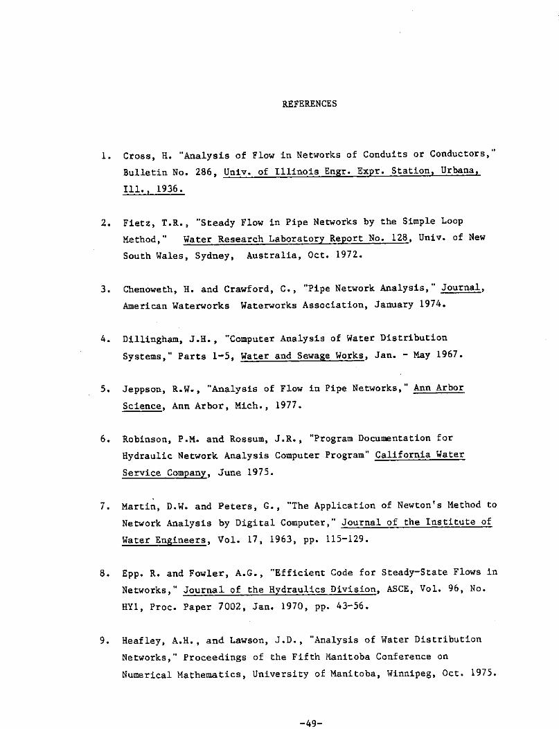
REFERENCES
l. Cross, H. "Analysis of Flow in Networks of Conduits or Conductors,"
Bulletin No. 286, Univ. of Illinois Engr. Expr, Station, Urbana,
Ill., 1936.
2. Fietz, T.R., "Steady Flow in Pipe Networks by the Simple Loop
Method," Water Research Laboratory Report No. 128, Univ. of New
South Wales, Sydney, Australia, Oct. 1972.
3. Chenoweth, H. and Crawford, C., "Pipe Network Analysis," Journal,
American Waterworks Waterworks Association, January 1974.
4. Dillingham, J .H. , "Computer Analysis of Water Distribution
Systems," Parts 1-5, Water and Sewage Works, Jan. - May 1967.
5. Jeppson, R.W., "Analysis of Flow in Pipe Networks," Ann Arbor
Science, Ann Arbor, Mich,, 1977.
6. Robinson, P .M. and Rossum, J .R., "Program Documentation for
Hydraulic Network Analysis Computer Program" California Water
Service Company, June 1975.
7, Martin, D. w. and Peters, G., "The Application of Newton's Method to
Network Analysis by Digital Computer," Journal of the Institute of
Water Engineers, Vol. 17, 1963, pp. 115-129.
8. Epp. R. and Fowler, A.G., "Efficient Code for Steady-State Flows in
Networks," Journal of the Hydraulics Division, ASCE, Vol. 96, No.
HYl, Proc. Paper 7002, Jan. 1970, pp, 43-56.
9. Heafley, A.H., and Lawson, J.D., "Analysis of Water Distribution
Networks," Proceedings of the Fifth Manitoba Conference on
Numerical Mathematics, University of Manitoba, Winnipeg, Oct. 1975.
-49-

10. Wood, D.J. and Charles, C.O.A., "Hydraulic Network Analysis Using
Linear Theory," Journal of the Hydraulics Division, ASCE, Vol. 98,
No. HY7, Proc. Paper 9031, July 1972, pp. 1157-1170.
11. Fietz, T.R., "Steady Flow in Small Pipe Networks Using Linear
Theory," Water Research Laboratory Report No. 130, Univ. of New
South Wales, Sydney, Australia, Jan. 1973.
12. Wood. D.J., "Users Manual - A Computer Program for the Analysis of
Pressure and Flow in Pipe Distribution Systems," Office of Engr.
Cont. Education, Univ. of Kentucky, Lexington, Kentucky, 1974,
(Revised 1975, 1977, and 1979).
13. Shamir, U. and Howard, C.D,D., "Water Distribution Systems
Analysis," Journal of the Hydraulics Division, ASCE, Vol. 94, No.
HYl, Proc. Paper 5758, Jan. 1968, PP• 219-234.
14. Lemieux, P .F., "Efficient Algorithm for Distribution Networks,"
Journal of the Hydraulics Division, ASCE, Vol. 98, No. HYll, Proc.
Paper 9336, Nov. 1972 pp. 1911-1920.
15. Liu, K.T.H., "The Numerical Analysis of Water Supply Networks by
Digital Computer," Proceeding, 13th Congress of the International
Association for Hydraulic Research, Vol. 1, Subject A. Sept. 1969,
PP• 35-42.
16. Barlow J.F. and Markland, E., "Computer Analysis of Pipe
Networks," Proceedings I.C.E., Vol. 43, June 1969, pp. 249-259.
17. Fietz, T .R., "Steady Flow in Pipe Networks by the Simple Loop
Method," Water Research Laboratory Report No. 128, Univ. of New
South Wales, Sydney, Australia, Oct. 1972.
-50-

18, Hoag, L,N, and Weinberg, G., "Pipeline Network Analysis by
Electronic Digital Computer," Journal of the American Water Works
Association, Vol, 49, 1957, pp. 517-524.
19. Collins, M.A., and Kennington, J. L., discussion of "Extended Period
Simulation of Water Systems--Part B." by H,S, Rao, L.C. Markel, and
D,W. Brue, Jr., Journal of Hydraulic Division, ASCE, Vol, 103, No.
HY12, Proc. Paper 13378, Dec, 1977, pp. 1496-1500,
-51-

The following symbols are used in this paper:
A
c
D
f
g
H
j
K
K p
JI,
L
M
n
ff p
N
P(Q)=
=
=
=
=
=
=
=
=
=
=
=
=
=
=
=
=
=
=
=
=
=
=
=
=
=
=
line area
Hazen Williams Roughness Coefficient
line diameter
energy input by pump
number of fixed grade nodes
gravitational constant
gradient for head change based on approximate flowrate
energy loss due to minor losses
energy loss in pipe section
energy loss due to wall shear
grade (head) at junction node
head change in pipe section based on approximate flowrate
useful horsepower for pump
number of junction nodes
loss coefficient for pipe section
loss coefficient due to minor losses
loss coefficient due to line loss
number of primary loops
line length
minor loss coefficient
exponent for head loss expression
number of pumps in system
number of nodes adjacent to given node
number of FGN's adjacent to given node
number of variable grade nodes adjacent to given node
number of pipes, in system
function for pump description (depends on flowrate, Q)
-5~2-

Q = flowrate in pipe section
Qe = enternal flowrate at junction node
Qf = flowrate in pipe section after adjustments
Qi = flowrate in pipe section prior to adjustments
Qin = flowrate into junction node
Qout = flowrate out of junction node
z = ccn st ant for constant power pump description
" = constant for pump description SN method
a = constant for pump description - SM method
ll.E = constant grade difference for energy equation
ll.H = grade adjustment for N and SN methods
ll.Q = flow adjustment for P and SP methods
The following subscripts are used for flowrates, Q, grades, H, and loss coefficiaits, K:
a, b, c, d
j, k
1, 2, 3, 4, 5, 6, 7, 8

APPENDIX
Computer Programs - Common Information
The computer programs which are appended were written to illustrate the application of the various algorithms to pipe network analysis. Each program is written assuming that for a system of P pipes and J junction nodes, the pipes are numbered from l to P and the data is input in this order and the junction nodes are numbered from l to J and input data for junction nodes, if required, is input in this order. Some notation is common to the five programs. This is summarized below. The first eight items are input data for all programs.
P - number of pipes in pipe system J - number of junction nodes in system Cl - flow conversion factor (f3/s to units used) Ll - length of pipe section (ft) Dl - diameter of pipe section (in.) Rl - Hazen Williams Roughness Coefficient Ml sum of minor loss coefficients in pipe section Pl - useful horsepower for pump X - exponent for head loss equation - 1.852 D(N) - diameter fo pipe Nin feet (Dl/12) Z(N) - pl.llllp energy term for pipe N - Pl(SS0/624) Q(N) - flow rate in pipe N H(N) - grade at junction node N Q8 - sum of absolute changes in flowrate between trials Q9 - sum of absolute"flowrates for trial QS - relative change in flowrate between trials TS - trial counter
Additional notation will be defined for each sample program. The input data requirements depend on the algorithm used and are summarized for each program.
Each program uses the same criterion for terminating the calculations and this occurs when the relative change in flowrate (absolute) between the last two trials is less than .1 percent. This is
where i refers to the last trial and i-1 to the next to the last trial.
Each program is used to analyze five examples which appear in the USERS MANUAL and the flowrates and grades obtained for these examples are output along with an indication of the convergence characteristics of each solution as the solution trials are carried out. Schematics for these examples were also appended. For systems with pumps, useful power is given.
The solution obtained by the various algorithms are in quite good agreement althourh some discrepancies occhr. The solutions obtained by the linear method are the most accurate ones.
-54-

t
"' .. a.
0 <O
- -200• • 4• 200'- 4' so'-_ 4 •
IA: C•IIO(Al.L.PIPES) 0
SG • I.O(WATER)
-.. I b t <@)
/6.
Example I
0 .. STORAGE TANK
Distribution system fed by large pressure main - required discharge pressures specified. p=7, L=O, j=2, t=6
C • 100 (all pipes)
2000'- 14' 4cfs.
• :t • !:
8 "' "'
2cfa. 3000• • 14 •
2cfs.
Example 2A Fourteen pipe distribution system changes for second analysis shown in ( ). English units p=14, L=3, i=B. t=4
Schematics - Examples cc

@ 3801 .. "
510'- 2'
© ® @)
• N
b N ., • m @
635 1- 4• 615'-4• @)
@) H.P., SU • ...
-., .,.,, o,
a>
"' ... [II • ® d· 'I, '!,~
@ ® @)
• N
-· . .!!:! ...
Hazen Wiiiiams Coefficient C• 130 for all pipes
Qdenotes sprinkle~-M~23
Example 4 17 pipe tree type watering system. p= 17, t=O, j=8, t= 10
5C.F.S.
,o ooo'- 2.4"
H.P.• 1950
,, ..
2 cf1
... 2200-I,
g "' ...
2C.F.S.
• N
~ "' .,
(@:)
.4 C.F.S .
4C.F.S.
C • 110 ( ALL PIPES)
Example 5A 17 pipe wot er distribution sys tern. p= 17, L = 4, j = 12, t = 2
Schematics - Examples (cont.)

.Junction 4
@ Regulator
p•50pslg
~ 0 o.
-o.
@
• 2 b 0
"'
® • 0
b "' ...
C•l20 (cllpipol
2CFS
4001 10• 600 1 10· I CFS
@ <@)
• 2 • "' b b
0 0
"' "' 4~0· 10·
2 CFS I CFS
<@.') sso' a• @ • "' ·o 0 ...
1000 1 10· I CFS
@
• • ,o .,o Exam pie 6 , ... Low pressure system -connected
to high pressure system (example 5 l ot junctions 4 and 5. p=!2, L=3, j=S, t=2
® Junction 5 regulator pa 50 pslg
Schematics - Examples (cont.)

Computer Programs - Loop Equations
The BASIC programs written for algorithms based on the loop equations are very similar and use some additional coIIL~on nomenclature. This is:
P2 O(N) C(N) G2 E(N) Gl
Hl
Ql I T(N) W(N, M)
- number of paths (£ + f - 1) - KM (Equ. 8) for pipe N - ~ (Equ. 6) for pipe N
grade at a reference fixed grade node - energy difference for path N - Gi (gradient for pipe section based on Qi,
Equ. 19) - Hi (head change for pipe section based on
Qi, Equ. 18) - absolute value of the flowrate - absolute value of pipe number - head change for pipe section N - array for storing geometric data
The W(N, M) array stores the required geometric data for the network and the required data depends on the algorithm used. For all methods it is necessary to know the flow direction in each pipe section at all times because the required. head summations depend on the flow direction in the pipe sections. This is done by designating an assumed flow direction in each pipe section. If the algorithm requires an initial flow assumption then the assumed flow direction is in the direction of the initial value used. If an assumed initial flowrate is not required an arbitrary direction is assumed. The initial assumed direction is indicated on the numbering schemes included with the computer results for each example. As the calculations are carried out, the direction of the flowrate is positive if it is in the initial assumed direction and negative if it reverses directions. Input geometric data requires a sign based on the initial assumed flow direction in order to specify the direction assumed. For example, all algorithms require input data specifying assigned pipe numbers for the paths of pipe sections making up primary loops and between fixed grade nodes. The pipe numbers are input with a postiive sign if the assumed flow direction is in the path direction taken to input the data and with a negative sign if it is not. This is illustrated using the loop shown below with a path direction (clockwise) as sepcified and the assumed flow directions noted. The data input would be 10,7,-6,8,-3. Additional sign convention for input geometric data are noted in the discussions and data specifications for the various algorithms.
~ 10
3
8
7
6 :,.,;v-
-58-
:\

APPENDIX 1 - Single Path Adjustment Method
The BASIC program uses the procedure described in pages 6-7 and the listing that follows. Additional pertinent notation used in the program is defined below with reference to the program line where it is first used.
270 Y(N)
330 Y (NJ 430 Bl 440 Al 530 Q2
number of pipes in path between junction N and junction N-1 number of pipes in path N numerator for flow correction factor (Equ. 21) denomenator for flow correction factor (Equ. 21) i'>Q (Equ. 21)
Note in line 510 the initial head changes, Hi, are added algebraicly and the correct sign is obtained by multiplying the head change by the flowrate and pipe number (with sign) and dividing by the absolute values of those quantities.
The data requirements are summarized below. An initial flowrate which satisfies continuity is required and the flow direction for these assumed flowrates are indicated on the example schematics. Pipe numbers are input for paths of pipes for the energy equation and paths of pipes between junction nodes and these are input with a positive sign if the initial flow direction is in the path direction and negative if it is opposite.
The required data is:
1 first line: no. of pipes, no. of junction nodes, flow conversion factor
2 next P lines (one for each pipe section): . length (ft), diameter (in), roughness, l: minor loss coefficients, useful pump power, initial flowrate
3 next line : reference grade for grade calculations, number of pipes from reference grade to junction node #1, pipe numbers (with sign) in path from reference grade to junction node #1 (repeat for each pipe), number of pipes between junction node #1 and #2, pipe numbers (with sign) in path from junction node #1 to #2 (repeat for each pipe), repeat last two items for each junction node in pipe system
4 next P-J lines (one for each energy equation). energy difference between starting and ending node (zero for loop), number of pipes in path, pipe numbers (with sign) in path from starting to ending node
The program listing and examples follow:

BASIC LISTING- SINGLE PATH ADJUSTMENT METHOD 100 DIM D<20),C<20),0<20>,Z<20>,V{20) 110 DIM E(20),Qi20>,HC20)1T<20),Y(20) 120 DIM W<20,20) 130 READ P,J,C1 140 P2=P-J 150 X•l.852 160 FOR N=l TO P 170 READ L1,D1,Rl,M1,P1,Q(N) 180 QCN)=Q(N)/Cl 190 D(Nl=Dl/12 200 Q(N)=.02S17tH1/DCN>**4 210 CCN)=4.73*L1/(R1**X*D<N>**4•87} 220 Z<Nl .. P1*550/62.4 230 VCN)=-QCN) 240 NEXT M 250 READ G2 260 FOR N=t TO J 270 READ YCN) 280.FOR M=1 TO YCN) 290 READ tJ<N,M> 300 NEXT M 310 NEXT N 320 FOR N•J+l TOP 330 READ ECN>,YCN) 340 FOR M=l TO Y<N> 350 READ W<N,M) 360 NEXT M 370 NEXT N 380 PRINT'TRIAL NO, RELATIVE FLOW CHANGE AVERAGE FLOW CHANGE' 390 FOR T5=1 TO 100 400 QB=O 410 Q9 .. 0 420 FOR N=J+t TOP 43'0 Bl=-E<N> 440 Al=O 450 FOR H•l TO Y(N) 460 I=ABS<W<N,M)) 470 Ql=ABS(O<I>>' 480 Gl=X*C(Il*01**CX-1)+2*D<I>*01+Z<Il/01**2 490 H1•C(ll*01**X+O<I>*01**2-!Cll/01 500 A1=A1+G1 510 B1•B1-H1*W<N,Ml*O(ll/(01*1) 520 NEXT M 530 Q2•B1/A1 540 FOR M•l TO Y<N) 550 I•ABSCWCN,H)) 56o_a(I)=Q(I)+02*W<N,M)/I 570 NEXT M 580 NEXT N 590 FOR N•1 TO P 600 Q8•08+ABS<ABS(O(Nll-ABS(V<N))) 610 09•09+ABS(O(Nll 620 VCN>=-G<NJ 630 NEXT N 640 IJ5=08/Q9 650 08=08*C1/P 660 PRINT T5,G5,GS 670 IF 05<,001 GO TO 690 680 NEXT T5
·690 FOR N•i TO? 700 Ql=ABS<O<N)) 710 T(Nl=O(Nl*<C<Nl*01**<X-1l+O(N)*Oll-Z(Nl/O(Nl 720 NEXT N 730 FOR N=l TO J 740 FOR M=1 TO Y(N) 750 I=ABS<W<N,Mll 760 G2:G2-T(I)*IIW<N,M) 770 NEXT H 780 H<N)=G:? 790 NEXT N 800 PRINT 810 PRINT 820 PR!NT•F'IF•E NUMBER FLOtJRATE• 830 FOR N=l TOP 840 D<N>=Cl*ABS(Q(Nl) 850 PRINT N,tJ(N) 860 NEXT N 870 PRINT 880 PRINT 'NODE NUMBER 890 FOF< N= 1 TO J 900 PRINT N,H(N) 910 NEXT N
GRADE•

TRIAL NO, RELATIVE FLOW CHANGE AVERAGE FLOW CHANGE
1 .269477 63,3179
2 6,07418E-02 14,4689
3 1. 75503E-<)2 4.18537
4 5.54139E-03 1,31961
5 t.47662E-03 .3514.39
6 3.21299E-04 7.64595E-02
920 DATA 7,2,448.86
PIPE NUMBER FLOWRATE 930 DATA 200,4,110,0,0,500
1 608.556 940 DATA 1so,2,110,2,o,100
2 95.~9 950 DATA 200,4,110,0,0,300
3 448,674 960 DATA 100,2,110,11,0,100
4 82 .193 970 DATA 200,2,110,6,0,100
5 64.2974 980 DATA 300,2,110,4,0,100
6 80.5535 990 DATA B0,4,110,3,0,100
7 285.928 1000 DATA 188.46,1,1,1,3 1010 DATA 102.3,2,1,2
NODE NUMBER GRADE 1020 DATA 123.84,3,t,3,4
1 130,434 1030 DATA 99.23,3,1,3,7
2 97.4365 1040 DATA 155.39,3,1,3,6 1050 DATA 88.46,2,1,5
Ea• 86.15 B
C Ec•64.62
_g_ l l~ NUMBERING A l CD 3 ® D
SCHEME EA•IBB.46 :z Ee• 89.23
jl! I ..§
EF • 100 F E EE• 33.08
Example 1 - Single Path Adjustment Method

TRIAL NO, 1 2 3 4 5
PIPE 1 2 3 4 5 6 7 8 9 10 11 12 13 14
NODE 1 2 3 4 5 6 7 8
NUMBER
NUMBER
RELATIVE FLOW CHANGE 7,82287E-02 3,36596E-02 4.10239E-03 1,00661E-03 4,61483E-04
FLOWRATE 9.65522 5.2743 1,2743 0.24794E-02 1,93752 3.36247 4,9054 3,88695 9,11653 4,38092 2.11722 ,575045 18,7716 3,22958
GRADE 202,543 133.575 104,774 103,046 103.04 119.833 106,58 136,198
AVERAGE FLOW CHANGE ,383143
13
, 16466 2.00776E-02 4.92770E-03 2,25960E-03
1240 DATA 14,B,1 1250 DATA 2000,14,100,8,0,9 1260 DATA 3000,14,100,0,0,5 1270 DATA 2500,14,100,0,0,1 1280 DATA 2000,14,100,0,0,.5 1290 DATA 2000,14,100,i0,0,1.5 1300 DATA 1500,12,t00,0,0,3 1310 DATA 2000,14,100,0,0,5 1320 DATA 3000,14,100,0,0,4 1330 DATA 2500,14,100,0,0·9 1340 DATA 2000,14,100,0,0,4 1350 DATA 100,0,100,0,0,1.s 1360 DATA 200,6,100,10,0,.5 1370 DATA 5000,16,100,S,1000,18 1380 DATA 3200,12,100,0,0,3 1390 DATA 10,1,13,1,1,1,2,1,3,1,4,2,-4,-7,1,6,2,-6,-8 1400 DATA 0,4,1,10,-8,-9 1410 DATA 0,4,2,3,-7,-10 1420 DATA 0,4,7,4,-5,--6 1430 DATA -90,5,tJ,1,2,3,11 1440 DA Tr; -100,3,13,9,14 1450 DATA -100,5,13,1,10,6,-12
2 @
i 311 aEe•IOO
© i 4
Ec•IIO ® Eo •110 0 5
NUMBERING SCHEME
Example 2 - Single Path Adjustment Method

TRIAL NO. RELATIVE FLOW CHANGE AVERAGE FLOW CHANGE 1 6.26541E-02 10.6004 2 2+32765£-02 3.94101 3 1.29302£-02 2.18964 4 8.09564E-03 1.37038 5 4.88977E-03 ,827152 6 2.87395E-03 ,485851 7 1+80289E-03 ,304653 8 1.23531E-03 .208695 9 9.16092E-04 ,154755
PIPE NUMBER FLOWRATE 1 635,671 1460 DATA 17,8,448,86 2 105,634 1470 DATA 635,4,130,0,54,2,600 3 52,4156 1480 DATA 520,2,130,5,0,100 4 53,218 1490 DATA 380,2,130,23,0,50 5 530,041 1500 DATA 510,2,130,23,0,50 6 325,386 1510 DATA 615,4,130,Q,QpSQO 7 204,667 1520 DATA 425,4,130,0,0,300 a 108,839 1530 DATA 385,4,130,10,0,200 9 95,8279 1540 DATA 195,2,130,23,0,100 10 160,563 1550 bATA 270,2,130·23,0,100 11 164.824 1560 DATA 540,4,130,2,0,t50 12 87.8722 1570 DATA 335,4,130,0,0,150 13 72.6905 1580 DATA 210,2,130,23,0,75 14 55.4857 1590 DATA 415,2,130,23,0,75 15 109,338 1600 DATA 375,2,130,23,0,50 16 52.5974 1610 DATA 255,4,130,0,0,100 17 56.7408 1620 DATA 180,2,130,23,0,50
1630 DATA 200,2,130,23,0,50 NODE NUMBER GRADE 1640 DATA 100,1,1,1,2,2,-2,5,1,7,2,-7,6,1,10,2,-10·11,1,15
1 290.753 1650 DATA -20,3,1,2,3 2 155.302 1660 DATA -10,3,1,2,4 3 189.361 1670 DATA 20,4,1,5,7,8 4 174.228 1680 DATA 15,4,1,5,7,9 5 160,978 1690 DATA 20,5,1,5,6,10,13 6 150,708 1700 DATA 15,5,1,5,6.·10,12 7 154,63 1710 DATA -15,5,1,5j6,11,14 8 152.37 1720 DATA -30,6,1,5,6,11,15,16
1730 DATA -25,6,1,5,6,11,15,17
B 3 @ 4
""" -- c
I 2 H
~ @ 6
A ~
© ..... I i 7 @) 9
8:;-©- E I D
13
NUMBERING SCHEME J
Example 4 - Single Path Adjustment Method

TRIAL NO. RELATIVE FLOW CHANGE AVERAGE FLOW CHANGE 1 .331088 2.36868 2 ,141433 .907504 3 8.27044E-02 .508281 4 4.39672E-02 .266733 5 1.78693E-02 .108027 6 6.32577E-03 3.81919E-02 7 2.16323E-03 t.30:548E-02 8 7,37755E-04 4.45161£-03
PIPE NUMBER FLOWRATE 1 29.6052 2 16.4996 3 6,16067 4 2.60526 1740 DATA 17,12,t s 3.55541 1750 DATA 10000,24,110,10,1950,40 6 .496099 1760 DATA sooo,1s~110,o,o,2s 7 4.4961 1770 DATA 5000,16,110,0,0,15 8 1.41175 1780 DATA 1000,6,110,5,0,13 9 .588243 1790 DATA 5500,14,110,0,0,2 10 2.58824 1800 DATA 3soo,12·,110,o,o,1 11 8.5173 1810 DATA 5500,14,110,0,0,5 12 13.1055 1820 DATA 4500,12,110,0,0,1 13 5,33903 1830 DATA 2500,6,110,0,0,1 14 2.60945 1840 DATA 3500,12,110,0,0,3 15 2.94848 1850 DATA 2200,1s,110,o,o,10 16 5.15128E-02 1860 DATA 6500,18,110,Q,0,15 17 ·2 1870 DATA 5000,14,110,0,0,5
1880 DATA 5300,12,110,0,0,4 NODE NUN BER GRADE 1890 DATA 3000,14,110,0,0,4
l 474.483 1900 DATA 4000,12,110,0,0,1 2 376.676 1910 DATA 4000,16,ito,o,o,2 3 348,679 1920 DATA 50, 1, 1, 1,2-, 1,3, 1,5, 1,-6,2,6,-16 4 327.359 1930 DATA 1,-15,1,-14,1,8,1,-9,1,-10,1,17 5 328.108 1940 DATA 0,5,2,13,-14,-11,-1~ 6 327.346 1950 DATA 0,5,3,S,-16,-15,-13 7 335,568 1960 DATA 0,5,15,L6,-6,-7,14 8 361.037 1970 DATA 0,4,11,8,-9,-10 9 354,357 1980 DATA -150 ,4,1,2,3,4 10 375,804 11 391.769 12 388,98
B i::.· 200
@
NUMBERING SCHEME
Example 5 - Single Path Adjustment Method·

TRIAL NO, 1 2 3 4 5 6
PIPE NUMBER 1 2 3 4 5 6 7 8 9 10 11 12
NODE NUMBER 1 2 3 4 :; 6 7 B
RELATIVE FLOW CHANGE AVERAGE FLOW CHANGE .434211 .727235 .159398 .264427 4.35456£-02 7.13925£-02 1.25796£-02 2.05487E-02 2.82026£-03 4.60345£-03 5,78349E-04 9,43894E-04
FLOWRATE 4.29332 3.0762 ,891887 1060 DATA 12,8,1 ,108113 1070 DATA 1500,10,120,0,0,3 ,631613 1080 DATA 400, 10, 120, 0, 0, 2 1,63161 1090 DATA 600,10,120,0,0,1+6 1,07506 1100 DATA 800,8,120,0,0,.6 2.29218 1110 DATA 700,8,120,0,0,1.5 ,476499 1120 DATA 1000,10,120,0,0,2.5 ,184317 1130 DATA 750,10,120,0,0,t.5 1.21711 1140 DATA 450,10,120,0,0,2.5 3,70668 1150 DATA 550,9,120,0,0,1.1
1160 DATA soo,10,120,0,0,1.6 GRADE 1170 DATA 800, 10, 120,0,0, 1
239.251 1180 DATA 1450,10,120,0,0,5 234+055 1190 DATA 275,38,1,1,1,2,1,3,1,4,1,9,1,-8,1,-7,1,6 233.268 1200 DATA 0,4,2,-10,-8,-11 233,33 1210 DATA 0,4,3,4,9,10 234, 1220 DATA 0,5,8,-9,-5,-6,7 237,39 1230 DATA 10,4,1,11,-7,-12 239.78 234.766
E• • 275.38 A
PR
~I
0 2 ® 3 @ ~ ~
I II 1 10 1 4
© a 9 © ~ ® 1 7 5 -0 6 ©
12~ NUMBERING SCHEME
B E9 • 265.38
Example 6 - Single Path Adjustment Method

APPENDIX 2 - Simultaneous Path Adjustment Method
The BASIC program which is listed on the next page uses the procedure described on pages 7-8. Additional pertinent notation used in the program is defined below along with reference to the program number where is it first used.
170 MATA 180 MATR 190 MAT B
200 MATG 290 V(N) 330 Y(N)
390 Y(N) 390 U(N) 510 Nl 590 Al 600 Bl 670 Il 680 I2 720 A(Nl, Il)
coefficient matrix for flow adjustment equations inverse of A constant matrix (vector) for right side of flow adjustment equations solutions of flow adjustment equations (6Q's) initial flowrate for pipe section N(Q.) number of pipes in path between junction node N and N-1 number of pipes in path N number of pipes common to other paths path number l:Gi for path Nl (also A(Nl, Nl))
- 6E - l:Hi for path Nl (also B(Nl, 1)) path number for common pipe pipe number for common pipe contribution from path Il to flow adjustment for path Nl
Note in lines 600.and 720 contributions are added algebraically depending on assumed flow directions and path directions.
The data requirements are summarized below. An initial flowrate which satisfies continuity is required and the flow direction for these assumed flowrates are indicated on the example schematics. Pipe numbers are input for paths of pipes for the energy equation and paths of pipes between junction nodes and these are input with a positive sign if the initial flow direction is in the path direction and negative if it is opposite. For each path, path numbers (with a sign) and pipe numbers are input for all pipes common to other paths and the path number is input with a positive sign if the two paths are in the same direction with respect to the common pipe.
The required data is:
1. first line: no. of pipes, no. of junction nodes, flow conversion factor
2. next P lines (one for each pipe section): length (ft), diameter (in), roughness, i: minor loss coefficients, useful pump power, initial flowrate
3. next line : reference grade for grade claculations, nur.ber of pipes from reference grade to junction node #1, pipe numbers

(with sign) in path from reference grade to junction node #1 (repeat for each pipe), number of pipes between junction node #1 and #2, pipe numbers (with sign) in path from junction node #1 to #2 (repeat for each pipe), repeat last two items for each junction node in pipe system
4. next P-J lines (one for each energy equation): energy difference between starting and ending node (zero for loop), number of pipes in path, number of pipes common to other paths, pipe numbers (with sign) in path from starting to ending node, path number (with sign) for common pipe, pipe number for common pipe (repeat last two items for all common pipes in path).
A program listing and examples follow.
BASIC LISTING - SIMULTANEOUS PATH ADJUSTMENT METHOD
100 DIM A(20,20>,R(20,20),B<20,1),G(20,1) 110 DIM D<20>,CC20>,0C20),Z(20),U{20) 120 DIM U(20) 130 DIM EC20),0(20),H(20),T(20),Y(20) 140 DIM IJ(20,20l 150 READ P,J,Cl 160 P2=P-J 170 HAT A =ZERCP2,P2) 180 MAT R =ZER<P2,P2) 190 MAT B =ZERCP2,1) 200 MAT G =ZER<P2,1) 210 X=l.852 220 FOR N=l TOP 230 READ L1,D1,R1,Ml,P1,Q(N) 240 G(N)=Q(N)/Cl 250 D<N>=Dl/12 260 OCN>=.02517*M1/D(N)**4 270 C CN l =4. 73*Ll./ < Rl**X*I• < N l 04, 87 l 280 ZCN)=P1*550/62.4 290 V CN l =Q CN l 300 NEXT N 310 READ G2 320 FOR N=l TO J 330 READ Y <N l 340 FOR M=l TO Y(N) 350 READ WCN,M) 360 NEXT M 370 NEXT N 380 FOR N=J+l TO F' 390 READ E(Nl,Y(N),UCN) 400 N1=YCN)f2*UCN) 410 FOR M=l TO Nl 420 READ lJCN,M) 430 NEXT M 440 NEXT N
. 450 PRINT"TRIAL NO. RELATil)E FLOW CHANGE AVERAGE FLOLJ Cl·IANGE• 460 FOR T5=1 TO 20 470 MAT A =ZER(F'2~F'2) 480 08=0 490 09=0
-67-

500 FOR N=J+l TOP 510 Nl=N-.J 520 :E(l=E(N} 530 Al=O 540 FOR M=l TO Y<N> 550 I=ABS(W(N~M)) 560 Ql=ABS(Q(I)) 570 Gl=X*C<I)*Q1**CX-1>+2*0(t)*Q1+Z(I)/01**2 580 H1=C<I>*01**X+O<I>*01*%2-Z<l)/Q1 590 Al=Al+Gl 600 11=B1-H1*W<N,M>*O<I)/IQ1*I> 610 NEXT M 620 A(Nl,N1)=A1 630 B<Nl,l>=Bl 640 N'2=Y(N>+1 650 N3=Y(N)t2*U(N) 660 FOR M=N2 TO N3 STEP'::? 670 Il=W<N,M) 680 I2=tJ(N,Mt1) 690 I=ABS(I2> 700 Ql=ABS<a(!)) 710 G1=X*CII>*01**1X-1)+2*0<I>*Q1+Z(l)/Q1**2 720 ACN1,I1>=A(N1,I1>+G1*I2/I 730 NEXT M
.740 NEXT N 750 MAT R=INV<A> 760 MAT G=R*B 770 FOR N=J+l TOP 7BO Nl=N-J 790 FOR M=l TO Y(N) BOO I=ABS(W<N,M)) 810 Q<I)=Q<I>+G<Nl,l)*WIN,M)/I 820 NEXT H 830 NEXT N 840 FOR N=l TOP 850 QB=OB+ABS<ABS(Q(N)>-ABSCV(N))) 860 Q9=09+ABS<G<N>) 870 V<N>=Q<N> 880 NEXT N 890 QS=QB/09 900 QB=QB*C1/P 910 PRINT T5~Q5,08 920 IF Q5<,001 GO TO 940 930 NEXT T5 940 FOR N=l TOP 950 Ql=ABS(Q(N)) 960 TIN)=QIN>•<C<N)*01**<X-1)t0(N>*01)-ZIN)/QCN) 970 NEXT N 980 FOR N=l TO J 990 FOR M=l TO Y(N) 1000 I=ADS(W(N,M)) 1010 G2=G2-T(I)*I/W(N,M) 1020 NEXT M 1030 H<N)=G2 1040 NEXT N 1050 PRINT 1060 PRINT 1070 PRINT"PIPE NUMBER FLOWRATE' 1080 FOR N=l TOP 1090 Q(N)=Cl*ABSIOIN)> 1100 PRINT N,OIN) 1110 NEXT N 1120 PRINT 1130 PRINT •NODE NUME1F.f~ GRAUE• 1140 FOR N=l TO J 1150 PRINT N•H(N) 1160 NEXT N

TRIAL NO. RELATIVE FLOW CHANGE AVERAGE FLOW CHANGE 1 .346501 86.663 2 5.49169E-02 13.0842 3 1.33345E-03 ,317296 4 1.28497E-06 3.05762E-04
1170 DATA 7,2,448.86 PIPE NUMBER FLOWRATE 1180 DATA 200,4,110,0,0,500
1 608,524 1190 DATA 150,2,110,2,0,100 2 95.6187 1200 DATA 200,4,110,0,0,300 3 448.614 1210 DATA 100,2,110,11,0,100 4 82,1591 1220 DATA 200,2,110,6,0,100 5 64.2924 1230 DATA 300,2,110,4,0,100 6 80.5549 1240 DATA B0,4,110,3,0,100 7 .285.9 1250 DATA 188.46,1,1,1,3
1260 DATA 102.3,2,1,1,2,2,-2 NODE NUMBER GRADE 1270 DATA -13.85,2,2,-2,5,1,-2,3,-5
1 130.439 1280 DATA 35.38,3,2,-5,3,4,2,-5,4,-4 2 97,4503 1290 DATA 31.54,2,2,-4,6,3,-4,5,-6
1300 DATA -56.15,2,1,-6,7,4,-6
Eo•89.23
Example 1 - Simultaneous Path Adjustment Method
-69-
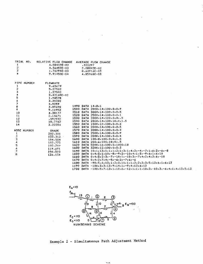
TRIAL NO. 1 2 3 4
PIPE 1 2 3 4 5 6 7 8 9 10 11 12 13 14
NODE 1 2 3 4 5 6 7 8
NUMBER
NUMBER
RELATIVE FLOW CHANGE AVERAGE FLOW CHANGE 6.58459E-02 .322297 4.26452E-03 2.08892E-02 1.76294E-03 8.6391.6E-03 9.91450E-04 4.85968E-03
FLOWRATE 9.65679 5.27502 1.27502 5,4214BE-02 1,94578 3.35285 4.9259 3,89698 9.11953 4,38177 2,14671 ,592932 18,7762 3.22254
GRADE 202.301 133.312 104.504 102.773 102,769 119.691. 106.508 136.134
1490 DATA 1500 ·DATA 1510 DATA 1520 DATA 1530 DATA 1540 DATA 1550 DATA 1560 DATA 1570 DATA 1580 DATA 1590 DATA 1600 DATA 1610 DATA 1620 DATA 1630 DATA 1640 DATA 1650 DATA 1660 DATA 1670 DATA 1680 DATA 1690 DATA 1700 DATA
Ee• 110
14,8,1 2000,14,100,8,0,9 3000,14,100,0,0,5 2500,14,100,0,0,1 2000,14,100,0,0,,5 2000,14,100,10,0,1,5 1soo,12,100,o,o,3 2000,14,100,0,0,5 3000,14,100,0,0,4 2500,14,100,0,0,9 2000,14,100,0,0,4 100,a,100,0,0,1.s 200,6,100,10,0,.5 5000,16,100,5,1000,18 3200,12,100,0,0,3 10,1,13,1,1,1,2,1,3,1,4,2,-4,-7,1,6,2,-6,-8 0,4,5,1,10,-8,-9,2,-10,4,1,5,-9,6,1,6,10 0,4,5,2,3,-7,-10,1,-10,3,-7,4,2,4,3,6,-10 0,4,2,7,4,-5,-6,2,-7,6,-6 -90,5,6,13,1,2,3,11,1,1,2,2,2,3,5,13,6,1,6,13 -100,3,3,13,9,14,1,-9,4,13,6,13 -100,5,7,13,1,10,6,-12,1,1,1,10,2,-10,3,-6,4,1,4,13,5,13
Eo•IIO
NUMBERING
Example 2 - Simultaneous Path Adjustment Method

TRIAL NO. 1 2 3 4
PIPE NUMBER 1 2 3 4 5 6 7 8 9 10 11 12 13 14 15 16 17
NODE NUMBER 1 2 3 4 5 6 7 8
.RELATIVE FLOW CHANGE AVERAGE FLOW CHANGE S.74509E-02 9.64187 1.Q6125E-O~ 1.79142 1+53770E-03 .259765 2+06060E-04 3.49134E-02
FLOWRATE 1710 DATA 17,8,448.86 635.783 1720 DATA 635,4,130,0,54.2,600 105.559 1730 DATA 520,2,130,5,0,100 52.3444 1740 DATA 380,2,130,23,0,50 53.2148 1750 DATA 510,2,130,23,0,50 539.223 1760 DATA 615,4,130,0,0,500 325,615 1770 DATA 425,4,130,0,0,300 204.609 1790 DATA 385,4,130,10,0,200 108,746 1790 DATA 195,2,130,23,0,100 95,9634 1800 DATA 270,2,130,23,0,100 160. 992 1810 DATA 540,4,130,2,0,150 164,633 1820 DATA 335,4,130,0,0,150 88.1425 1830 DATA 210,2~130,23,0,75 72.8398 1840 DATA 415,2,130,23,0,75 55.699 1850 DATA 375,2,130,23,0,50 108.934 1860 DATA 255,4,130,0,0,100 52.4047 1870 DATA 180,2,130,23,0,50 56.529 1880 DATA 200,2,130,23,0,50
1890 DATA 100,1,1,1,2,2,-2,s,1,7,2,-,,6,1,10,2,-10,11,1,1s .GRADE 1900 DATA -20,3,2,1,2,3,3,-2,2,-3 290.645 1910 DATA 10,2,2,-3,4,1,-3,3,-4 155.:5-72 1920 DATA 30,5,4,-4,-2,5,7,8,2,-4,1,-2,5,-7,4,-8 189, 189 1930 DATA -5,2,2,-8,9,3,-8,5,-9 174,063 1940 DATA S,5,3,-9,-7,6,10,13,4,-9,7,-10,6,-13 160,769 1950 DATA -5,2,2,-13,12,S,-13,7,-12 150,448 1960 DATA -30,4,3,-12,-10,11,14,6,-12,B,-14,5,-10 154,434 1970 DATA -10,3,2,-14,1S,f7,7,-14,9,-17 152 .189 1990 DATA -5,2,1,-17,16,8,-17
B 3 ® 4 c -....::: ....,...
I 2 H
' @ 6 A
<D ~ --..
j 7 ® 10 I
9 ",: I~ 8 v©~ E ©
0 j 13
NUMBERING SCHEME J
Example 4 - Simultaneous Path Adjustment Method

TRIAL NO, 1 2 3 4 5
PIPE NUMBER 1 2 3 4 5 6 7 8 9 10 11 12 13 14 15 16 17
NODE NUMBER 1 2 3 4 5 6 7 8 9 10 11 12
RELATIVE FLOW CHANGE ,274315 .125239 3.26663E-02 2.61657£-03 1,67876E-05
FLOWRATE 29.6046 16,5049 6,16393 2.60463 3,5593 .49289 4,49289 1,41217 .587826 2,58782 8,51183 13,0997 5,34104 2,60676 2,94781 5,21863£-0~ 2
GRADE 474,502 376,637 348,613 327,25 327,99 327,236 335.455 360.875 354,191 375,611 391.57 388.782
AVERAGE FLOW CHANGE 1.89649 ,778823 .197532 1,57874£-02 1,01288E-04
1990 DATA 17,12,1 2000 DATA 10000,24,110,10,1950,40 2010 DATA 5000,18,110,0,0,25 2020 DATA 5000,16,110,0,0,15 2030 DATA 1000,6,110,5,0,13 2040 DATA 5500,14,110,0,0,2 2050 DATA 3500,12,110,0,0,1 2060 DATA 5500,14,110,0,0,5 2070 DATA 4500,12,110,0,0,1 2080 DATA 2500,6,110,0,0,1 2090 DATA 3500,12,110,0,0,3 2100 DATA 2200,15,110,0,0,10 2110 DATA 6500,18,110,0,0,15 2120 DATA 5000,14,110,0,0,5 2130 DATA 5500,12,110,0,0,4 2140 DATA 3000,14,110,0,0,4 2150 DATA 4000,12,110,0,0,1 2160 DATA 4000,16,110,0,0,2 2170 ItATA so,1,1,1,2,1,3,1,s,1,-6,2,6,-16 2180 DATA 1,-15,t,-14,1,B,1,-9,1,-10,1,17 2190 DATA 0,5,4,2,13,-14,-11,-12,5,2,2,-13,3,-14,4,-11 2200 DATA 0,5,4,3,5,-16,-15,-13,S,3,3,-16,3,-15,1,-13 2210 DATA 0,5,3,15,16,-6,-7,14,2,-15,2,-16,1,-14 2220 DATA 0,4,1,11,8,-9,-10,1,-11 2230 DATA -150,4,2,1,2,3,4,1,2,2,3
E0 •200
NUMBERING SCHEME
Example 5 - Simultaneous Path Adjustment Method

TRIAL NO, 1 2 3 4 5
PIPE 1 2 3 4 5 6 7 8 9 10 11 12
NODE 1 2 3 4 s 6 7 8
NUMBER
NUMBER
RELATIVE FLOW CHANGE ,401845 .125886 4.35776E-02 3.94722E-03 6,10902E-05
FLOWRATE 4,29337 3,07668 .892329 , 107671 ,631427 1.63142 1.0752 2,29189 ,476243 , 184349 1,21669 3,70662
GRADE 239,25 234.052 233,265 233.327 233,996 237,385 238. 776 234.763
AVERAGE FLOW CHANGE ,690139
PR
B
.203871 7.12019E-02 6,44193E-03 9,96987E-05
1310 DATA 12,e,1 1320 DATA 1500,10,120,0,0,3 1330 DATA 400,10,120,0,0,2 1340 DATA 600, 10,·120,0·,-o-,----i ·,6 1350 DATA 800,8,120,0,0, .6 1360 DATA 700,B,120,0,0,1.5 1370 DATA 1000,10,120,0,0,2.5 1380 DATA 750,10,120,0,0,1,5 1390 DATA 450,10,120;0,o,2.s 1400 DATA 550,8,120,0,0,1.1 1410 DATA soo,10,120,0,0,1.6 1420 DATA soo,10,120,0,0,1 1430 DATA 1450,10,120,0,0,5 1440 DATA 275,38,1,1,1,2,1,3,1,4,1,9,1,-8,1,-7,1,6 1450 DATA 0,4,3,2,-10,-B,-11,2,-10,3,-8,4,-11 1460 DATA 0,4,2,3,4,9,10,1,-10,3,-9 1470 DATA 0,5,2,8,-9,-5,-6,7,1,-8,2,-9 1480 DATA 10,4,2,1,11,-7,-12,1,-11,3,-7
E• • 275.36 A
'\: I
© 2 ® 3 @ ~ ...,..
j II 1 10 l 4
© 6 9 © ....... ® -i 7 1 5 ~
0 6 ® 120 .
NUMBERING SCHEME
E 8 • 265.36
Example 6 - Simultaneous Path Adjustment Method
-73-

APPENDIX 3 - Linear Method
This program is based on the procedure given on page 8. The listing of the BASIC program for this is shown on the next page. Additional pertinent notation along with the line number where it first appears is defined below.
150 MATA 160 MATR 170 MAT B 180 !!,AT G 300 Nl 300 Fl 330 Pl 370 Y(N)
430 Y(N) 530 Bl
coefficient matrix for linear equations inverse of A constants for linear equations solution for flowrates (Q) number of pipes connecting at junction external demand or inflow at junction pipe number (with sign) connecting junction number of pipes connecting junction N to junction N-1 number of pipes in path N E(G.Q.-H.) Equ.21
1 1 1
The data requirements are summarized below. Pipe numbers are input for pipes connecting junction nodes, pipes in a path between junction nodes and pipes in a path for the energy equations. An assumed flow direction is made for each pipe section (as noted on the examples) and the following sign convention is applied. For pipes connecting a junction node the sign of the pipe number is input as negative for the assumed flow direction into the junction node and positive if it is out. For pipes in a path the sign of the pipe number is input as positive if it is in the path direction and negative if it is opposite.
The required data is:
1 first line: no. of pipes, no. of junction nodes, flow conversion factor.
2 next P lines (one for each pipe section): length (ft), diameter (in), roughness, t minor loss coefficients, useful pump power
3 one line: grade for reference
4 next J lines (one for each junction node): no. of pipes connecting node, external flowrate, pipe numbers (with sign) of pipes connecting this junction node, number of pipes in path connecting this junction node with last one input (reference grade for first junction node input), pipe numbers (with sign) of pipes in this path
5 next P-J lines (one for each energy equation): energy difference between starting and ending node (zero for loop), no. of pipes in path, pipe numbers (with sign) in path from starting to ending node
The program listing and examples follow.

lOO DIH A(20,20),R(20,20),B(20,1),G(20,1) 110 DIM D(20),C(20),0(20),Z(20) 120 DIM E<20),0(20),H(20),T(20),Y(20) 130 DIM W(20,10> l.40 READ P, .. J,Cl 150 MAT A =ZER\F',-P) 160 MAT R =ZERIP,Pl 170 HAT B :::ZER<P,1) 180 MAT G =ZER<P,1) 190 X=t.852 200 FDR N•• 1 TO P 210 READ L1,D1,Rl,M1,Pl 220 D(N)=J)1/12 230 OINl=,02517*Ml/DINl**4 240 CCN)=4.73ill/(R1**X*D<N>**4•87) 250 ZCN)=P1*550/62,4 260 QINl•3,1416*D1Nl*DIN) 2'/0 NEXT N 280 READ G2 2 170 FOR N:::1 TO J 300 F~EAD N1, F 1 310 BIN,1)=-Fl/Cl :320 FOf< Mao! TO Nl 330 READ Pl 340 .I:::ABS<P1> 350 A<N,Il•Plll 360 NEXT M 370 READ YIN) 380 FOR M•l TO YINI 390 RE:All WCN,Ml 400 NEXT M 410 NEXT N 420 FOR N•~tl TOP 430 READ E<N>,Y(N) 440 FOR M•l TO YIN) 450 REAi) W<N,M) 460 NEXT M 470 NEXT N 4BO PRINT"TRIAL NO. 490 FOR T5=1 TO 20 soo aa:::,o
RELATIVE FLOW CHANGE AVERAGE FLOW CHANGE•
BASIC LISTING - LINEAR METHOD
51() 09=0 520 FOR N=.ltl TO P 530 54() 5SO 560 570 580 590 600 610 620 630 640 650 660 670 680 690 700 710 720 730 740 750 760 770 780 790 EIOO 81() 820 El30 840 85() 860 870 800 El90 900 910 920 930 940 950 9b0 970 9DO
Bl=O FOR M=1 TO YIN> I=ABSIW(N,Hll e11~=t1ftS(O<I) > Gl•X*C<Il*G1**1X-1)+2*0<I)tGltZIIl/G1**2 Hl•CIIl*Ul**X+OIIl*01**2-ZIII/QJ A<N,I)=G1*WCN,M>II B1•Blt1Gl*OI-Hll*Glll*WIN,HI/IG1*I> NEXT M B<N,i>=Bl+E(N) NEXT N MAT R=INVIA) HAT G=R:t::B FOR N=l TOP 08•08tABSIABSIOIN)l-ABS(GIN,1l)) ll9=09+ABS 1G IN, 1) ) ll(N)=G<N,1) NEXT N l15=08/09 ClB=l10*Cl.lP PRINT T5,05,C18 IF G'.l<,001 00 TO 760 NEXT TS FOR N=l TOP fll=ABSIOINI) TIN)•01Nl*ICINl*l11**1X-llt01Nl*Gll-ZINI/GIN) NEXT N FOR N=I ,TQ J FOR M•1 TO YIN) I=ABS(W(N,M)) G2=G2-T(I>*WCN,M)/I NEXT M U < N > ==G2 NEXT N PRINT PRINT PRINT.PIP!:: NUMBER FllR N=l TOP QIN)•Cl*ABSIG(N)I PRINT N,O<NI NEXT N Pi:~INT PfUNT 'N0[1E NUHBER FOR N=l TO J ~-=-n:rNT N,H<N> NEXT N
FLOWf<ATE•
13RAnE•

TRIAL NO, RELATIVE FLOW CHANGE AVERAGE FLOW CHANGE 1 ,763143 288,47 2 ,449275 117,181 3 9.19791E-02 21,9694 4 3,72790E-03 ,88711 5 7,01801E-06 1.67022£-03
PIPE NUHBER FLOWRATE 1010 DATA 7,2,448.86 1 600,566 1020 DATA 200,4,110,0,0 2 95,61 1030 DATA 150,2,110,2,0 3 448,616 1040 DATA200,4,110,0,0 4 82.1092 1050 DATA 100,2,110,11,0 5 64,3402 1060 DATA 200,2,110,6,0 6 80.5695 1070 DATA 300,2,110}'4,0 7 205,936 1080 DATA 80,4,110,3,0
1090 DATA 188,46 NODE NUMBER GRADE 1100 DATA 4,0,-1,2,J,5,1,1
1 130.432 1110 DATA 4,0,-3,4,6,7,1,3 2 97.4426 1120 DATA 102.3,2,1,2
1130 DATA 123.8,3,1,3,4 1140 DATA 99.23,3,t,3,7 1150 DATA 155.4,3,1,3,6 1160 DATA aa.s,2,1,:s
E9 •86.15
.z B
C Ee• 64.62
'~ SCHEME
PR l. CD 3 2 A I t--::::::-=-r---::""""+'-"!"-- 0
:!. Eo • 89.23
NUMBERING
.§
Example 1 - Linear Method
-7F,-

TRIAL NO, 1 2 3 4 5 6
PIPE NUMBER 1 2 3 4 5 6 7 9 9 10 11 12 13 14
NODE NUMBER l 2 3 4 5 6 7 8
TIME 0 SECS,
RELATIVE FLOW CHANGE AVERAGE FLOW CHANGE ,996948 .554163 ,285895 1,86452E-02 .t .21S49E-03 1. 35507E-05
FLOWRATE 9,65666 5,27246 1,27246 3,44235E-02 1,96557 3,36371 4.91862 3,99913 9, 11977 4,3842 2,15665 ,601954 19,7764 3.22164
GRADE 202.294 133,306 104.525 102.a 102.799 119.672 106.41 136.124
Ee •110
Eo•IIO NUMBERING
2.52863 2.37176 1,41931 9+14687E-02 S.95961E-03 6.64395E-05
1500 DATA 1510 DATA 1520 DATA 1530 DATA 1540 DATA 1550 DATA 1560 DATA 1570 DATA 1590 DATA 1590 DATA 1600 DATA 1610 DATA 1620 DATA 1630 DATA 1640 DATA 1650 DATA 1660 DATA 1670 DATA 1680 DATA 1690 DATA 1700 DATA 1710 DATA ].720 DATA 1730 DATA 1740 DATA 1750 DATA 1760 DATA 1770 IIATA 1780 DATA 1790 DATA
Example 2 - Linear Method
-77-
14,8,t 2000,14,100,B,O 3000,14,100,0,0 2500,14,100,0,0 2000,14,100,0,0 2000,14, 100, 10,0 1500,12,100,0,0 2000,14,100,0,0 3000,14,100,0,0 2500,14,100,0,0 2000,14,100,0,0 100,s,100,o,o 200,6, 100, 10,0
5000,16,100,5,1000 3200,12,100,0,0 10 3,0,1,9,-13,1,13 3,0,-1,2,10,1,1 2,4,-2,3,1,2 4,4,-3,4,7,11,1,3 2,2,-4,5,1,4 4,0,6,-7,8,-10,2,5,-6 3,2,-5,-6,12,1,6 3,2,-B,-9,14,2,-6,8 0,4,1,10,8,-9 0,4,2,3,7,-10 0,4,-7,4,5,-6 -90,5,13,1,2,3,11 -10,-4,-11,4,5,12 0,4,-14,-8,6,12

TRIAL NO. RELATIVE FLOW CHANGE AVERAGE FLOW CHANGE 1 ./,19864 48.3676 2 .439292 61,1331 3 .171004 28.6778 4 7.40561E-03 1. 2512 s :5.53590E-05 9,35293E-03
PIPE NUMBER FLOWRATE 1800 DATA 17,8,448 .. 86 ! 635.787 1810 DATA 635,4,130,(),54.2 2 105,558 1820 DATA 520,2,130,5,0 3 52.3438 1830 DATA 380,2,130,23,0 4 53.2143 1840 DATA 510,2,130,23,0 5 530.229 1850 DATA 615,4,130,0,0 6 325.627 1860 DATA 425,4,130,0,0 7 204.603 1870 DATA 385,4, 130, 10,0 8 108.743 1880 DATA 195,2,130,23,0 9 95,8601 1890 DATA 270,2,tJ0,23,0 10 160,979 1900 DATA 540,4,130,2,0 11 164,648 1910 DATA 335,4, 130,0,0 12 88.1411 1920 DATA 210,2,130,23,0 13 72,8383 1930 DATA 415,2,130,23,0 14 55.7034 1940 DATA 375,2,130,23,0 15 108.944 1950 DATA 255,4,130,0,0 16 52.4102 1960 DATA 180,2, 130,23,0 17 56.5344 1970 DATA 200,2,130,23,0
1975 DATA 100 NODE NUMBER GRADE 1980 DATA J,0,-1,2,5,1,1
1 290.642 1990 DATA 3,0,-2,3,4,1,2 2 155.372 2000 DATA 3,0,-5,6,7,2,-2,5 3 189.183 2010 DATA 3,0,-7,8,9,1,7 4 174.059 2020 DATA 3,0,-6,10,11,2,-7,6 5 160.762 2030 DATA 3,o,-10,12,1J,t,10 6 150,441 2040 DATA 3,o,-11,14,1s,2,-10,11 7 154.426 2050 DATA 3,0,-15,16,17,1,15 8 152.181 2060 DATA -20,3,1,2,3
2070 DATA -10,3, 1,2,4 2080 DATA -3'0,6,l ,5,6",11,15,16 2090 DATA -25,6,t,S,6,11,15,17 2100 DATA -15,5,1,5,6,11,14 2110 DATA 15,5,1,5,6,10,12 2120 DATA 20,5,1,5,6,10,13 2130 DATA 15,4,1,S,7,9 2140 DATA 20,4,1,5,7,8
Example 4 - Linear Method
-78-

TRIAL NO. RELATIVE FLOW CHANGE AVERAGE FLOW CHANGE 1 .52431 2.6705 2 .200505 1.10147 3 .176449 1.13216 4 6.3J941E-02 .385538 5 9.16941E-03 5.53335E-02 6 2.02230E-04 1.22016E-03
PIPE NUMBER FLOWRATE 2150 DATA 17,12,1 1 29.6046 2160 DATA 10000,24,110,10,1950 2 16.5049 2170 DATA 5000,18,110,0,0 3 6, 16392 2180 DATA 5000,16,110,0,0 4 2.60463 2190 DATA 1000,6,110,5,0 5 J.55929 2200 DATA 5500,14,110,0,0 6 .492892 2210 DATA 3500,12,110,0,0 7 4.49289 2220 DATA 5500,14,110,0,0 B 1,41217 2230 DATA 4500,12,110,0,0 9 .587825 2240 DATA 2500,6,110,0,0 10 2.58793 2250 DATA 3500, 12, 110,0,0 11 8.51182 2260 DATA 2200,1s,110,o,o 12 13.0997 2270 DATA 6500,18,110,0,0 13 5.34103 2280 DATA S000,14,110,0,0 14 2,60676 2290 DATA 5500,12,110,0,0 15 2,9478 2300 DATA 3000,14,110,0,0 16 5.21917E-02 2310 DATA 4000,12,110,0,0 17 2 2320 DATA 4000,16,110,0,0
232'!"i DATA 50 NODE NUMBER GRADE 2330 DATA 3,0,-1,2,12,1,1
1 474,503 2340 DATA 3,5,-2,3,13,1,2 2 376.638 2350 DATA 3,0,-3,4,5,1,3 •. 3 348.613 2360 DATA 3,4,-5,6,-16,1,5 4 327.25 2370 DATA 2,4,-6,-7,1,6 5 327.99 2380 DATA 2,3,-15,16,2,-6,-16 6 327.237 2390 DATA 3,5,-13,-14,15,1,-15 7 335.455 2400 DATA 4,0,7,B,-11,14,t,-14 8 360.875 2410 DATA 2,2,-8,-9,1,8 9 354.192 2420 DATA 2,2,9,-10,1,-9 10 375,611 2430 DATA 4,0,10,11,-12,17,t,-to 11 391.571 2440 DATA 1,2,-17,1,17 12 388.782 2450 DATA O,S,2,13,-14,-11,-12
2460 DATA O,S,3,5,-16,-15,-13 2470 DATA 0,5,14,15,16,6,-7 2480 DATA 0,4,11,8,-9,-10 2490 DATA 150~4,-4,-3,-2,-1
8
E1 •200
NUMBERING SCHEM~.
Example 5 - Linear Method
_70_

TRIAL NO, 1 2 3 4
PIPE NUMBER 1 2 3 4 s 6 7 8 9 10 11 12
NODE NUMBER 1 2 3 4 5 6 7 8
RELATIVE FLOW CHANGE AVERAGE FLOW CHANGE .726257 , 111484 5,26916E-03 1,03049E-04
FLOWRATE 4.29337 3.07667 ,892328 .107672 .631429 1,63143 1.0752 2.29189 .476242 ,184349 1.21669 3.70662
GRADE 239.25 234.053 233.265 233.327 233.996 237,385 238,776 234,763
E• • 27e.3B A
t.18223 .181558 8,S9965E-03 1,68175E-04
2500 DATA 2510 DATA 2520 DATA 2530 DATA 2540 DATA 2550 DATA 2560 DATA 2570 DATA 2530 DATA 2590 DATA 2600 DATA 2610 DATA 2620 DATA 2630 DATA 2640 DATA 2650 DATA 2660 DATA 2670 DATA 2680 DATA 2685 DATA 2690 DATA 2700 DATA 2710 DATA 2720 DATA 2730 DATA 2740 DATA 3000 END
0 6 ® 12 '/ NUMBERING SCHEME
B E 1 • 26e.3B
Example 6 - Linear Method
12,8,1 1500, 10, 120, 0, 0 400,10,120,0,0 600,10,120,0,0 800,8,120,0,0 100,a,120,o,o 1000, 10, 120,0,0 750,10,120,0,0 450,10,120,0,0 550,8,120,0,0 800, 10, 120,0,0 000,10,120,0,0 1450,10,120,0,0 275,38 3,0,-1,2,11,1,1 3,2,-2,3,10,1,2 2,1,-3,4,1,3 3,1,-4,-5,-9,1,4 3,2,-8,9,-10,1,-9 3,0,-7,B,-11,1,-8 3,t,6,7,-12,1,-7 2,1,5,-6, 1,6 0,4,2,10,-8,-11 0,4,3,4,-9,-10 0,5,8,9,-5,-6,7 10,4,1,11,-7,-12

Appendix 4 Computer Program for Single Node Adjustment Method -Node Equations
The program listing (BASIC) which utilizes the procedure presented on pages .9 to 10 is shown on the next page. Additional pertinent notation along with the line number where it first appears is defined below.
140
180
195
210
220
260
300
300
330
420
440
450
460
600
610
Nl - number of pumps
U(N), V(N) - connecting nodes for pipe
O(N) - ZM F(N) - grade for pipe connecting fixed grade node
C(N) - KP (Equ. 6)
N2 - number of line with pump
Y(N) - number of pipes connecting junction node N
E(N) - external flowrate, junction node N
W(N, M) - pipes connecting junction node N
K(N) - loss coefficient pipe N (Equ. 23)
HS - summation of Grade Changes
QB - summation of flow changes
Q9 - summation of flows
QO - initial assumption - line with pump (Equ. 31)
Bl - denominator of Equ. 29
620 H4 - numerator of Equ. 29-
720 Al - ZQ (numerator of Equ. 28)
780 Bl - denominator of Equ. 28
The data requirements are summarized below. Pipes are numbered from 1 to P and junction nodes from 1 to J. Fixed grade nodes are numbered zero. The required data is:
1 first line: no. of pipes, no. of junction nodes, number of pumps, flow conversion factor
2 next P lines ( one for each pipe section): first node, second node, length (ft.), diameter (in.), roughness, Z minor loss coefficients, value for fixed grade if this pipes connects a fixed grade node (otherwise omit this data).
3 next line: repeat this pumps)
pipe number for line with pump, useful pump power, data for each pump (omit this line if system has no
-81-

4 next J lines (one for each junction node), number of pipes connecting this junction node, assumed grade for this node, external demand for this node, pipe numbers for pipes connecting this node.
The program listing and examples follow.
BAS>)'.C- t.ISTillG __ ~" .:.;i,:t,GLE NODE ADJUSTl:ENT ~iETHGD -- ·::--
100 DIH H(20),Z(20),B(20> 110 DIM U<20),V(20),D(20),C(20>,0(20> 120 DIH K<20>,E<20),Y(20),f(20> 130 DIM WC20,~),0(20> 140 READ P,J,Nl,Cl 150 T6•50 160 X=l .852 170 FOR N=l TOP 180 READ U<N),V<N>,Ll,D1,R1,M1 190 DCN>=Dl/12
-195 O<Nl=HI 200 IF U<Nl+V<N><>ABS(U<N>-V<N>> GO TO 220 210 READ F<N> 220 C(Nl=4,73*L1/(Rl**X*D<N>**4,87> 230 NEXT N 240 IF Nl=O GO TO 290 250 FOR N•l TO Nl 260 READ N2,Pl 270 Z<N21=P1*550/62,4 2BO NEXT N 290 FOR N•l TO J 300 READ Y<N>,H<N>,E<N> 310 E<N>=E<Nl/Cl 320 FOR H=I TO Y(N) 330 READ W<N,H) 340 NEXT H 350 NEXT N 360 TS•O 370 PRINT 'TRIAL NO, RELATIVE FLOW CHANGE AVERAGE HEAD CHANGE' 380 TS=T5+1 390 IF T5>T6 GO TO 970 400 FOR N•I TOP 410 Q3•ABS(Cl<N>l 420 K<N)=C(N)+,02517*0<N>*Cl3**•148/D<N>**4 "130 NEXT N 440 H8=0 450 08=0 460 09=0 470 FOR C=l TO J 480 Al=E<C> 490 B!=O 500 FOR H•I TO Y<C> 510 N=W<C,H) 520 J3=U<Nl+V(N>-C 530 Hl=H<C> 540 IF J3=0 GO TO 570 550 H2=H(J3> 560 GO TO 580 570 H2=F<N> 580 H3=ABS<H1-H2) 590 IF ZCN)=O GO TO 740 600 QO=CZCN)/KCN>l**(l/(l+X>> 610 B=l/CX*K<N>*OO**<X-1>+Z(Nl/U0**2l 620 H4=Hl-H2+ZCN)/DO-KCN>*OO**X 630 IF U<N>=C GO TO 650 640 H4=H2-Hl+Z(N)/OO-K<N>~OO*~X 650 Ql=H4*B 660 OO=l10+Dl 670 IF ABS(Qll>,001 GO TO 610 680 Bl=Bl+B
_Q')_

690 G<N>=GO 700 IF U(N>=C GO TO 720 710 G<N>=-00 720 A1=.Alt11<N> 730 GO TO 800 740 G(N>=<H3/KCN>>**<1IX> 750 IF H1>H2 GO TO 780 760 G(N>=-G(N) 770 IF H3=0 GO TO 790 780 B1=B1+<H3/K<N>>**(1/X-1l/<X*<K<Nlll 790 Al=AHIH N l 800 NEXT M 810 H<C>=H<C)-A1/B1 820 HB=H8+ABSCA1/B1) 830 NEXT C 840 FOR N=l TOP 850 IF T5=1 GO TO 890 860 07= ABS<G<Nll 870 G8=QB+G7 880 G9=G9+ABS<B<Nl-G7l 890 B<Nl=ABS<G<N)l 900 NEXT N 910 IF TS=1 GO TO 960 920 QS=09/ll8 930 H9=H8/J 940 PRINT T5,05rH9 950 IF GS<.001 GO TO 970 960 GO TO 380 970 PRINT 980 PRINT 990 PRINT 'PIPE NUMBER FLOWRATE' 1000 FOR N=l TOP 1010 G<N>=Cl*ABSCGCNl) 1020 PRINT N,G<N> 1030 NEXT N 1040 PRINT 1050 PRINT 'NODE NUMBER GRAUE' 1060 FOR N=l TO J 1070 PRINT N,H<Nl 1080 NEXT N
-83-

TRIAL ND, RELATIVE FLOW CHANGE AVERAGE HEAD CHANGE 2 3 4 5 6
PIPE 1 2 3 4 5 6 7
NODE 1 2
NUHBER
NUHBER
,202666 2.10941 5,10954E-02 .730122 9.05142E-03 ,119714 2.02572£-03 3.20134£-02 4,41792E-04 s.924t4E-03
FLOWRATE 1090 DATA 7,2J0,448.80 608,616 1100 DATA 0,1,200,4,110,0,188.46 95,612 1110 DATA 1,0,150,2,110,2,aa.15 448,653 1120 DATA 1,2,200,4,110,0 82.155 1130 DATA 2,o,100,2,110,11,64.62 64.2859 1140 DATA 1,0,200,2,110,0,100 80.5526 1150 DATA 2,0,300,2,110,4,33.08 285,84 1160 DATA 2,0,80,4,110,3,89.23
1170 DATA 4,140,0,1,2,3,5 GRADE 1180 DATA 4,100,0,3,4,6,7
130,431 97,4404
B Ea•B6.15 C Ec•64.62
~1 '~ NUMBERING A .1 CD 3 2 l--:::;--""''f-~~-1-=':!!'-D
SCHEME EA•ISB.46 .:t. Eo • 89.23
.2 j l!
Example 1 - Single Node Adjustment

TRIAL 2 3 4 5 6 7 8 9
PIPE 1 2 3 4 5 6 7 8 9 10 11 12 13 14
NODE 1 2 3 4 5 6 7 B
NO. RELATIVE FLOW CHANGE AVERAGE HEAD CHANGE
NUHBER
NUHBER
.221078 J.74231 7,14057E-02 1,69595 2.81430E-02 .713241 1,63690E-02 .256435 7.16994E-03 .111002 2.83070E-03 7.31062E-02 t.26856E-03 4.41590E-02 5.68328E-04- 2.54497E-02
FLOWRATE 1420 DATA 14,B,1,1 9.65339 1430 DATA 1,2,2000,14,100,B 5.27404 1440 DATA 2,3,3000,14,100,0 1.27564 1450 DATA 3,4,2500,14,100,0 t.5187SE..;.02 1460 DATA 4,5,2500,14,100,0 t.96641 1470 DATA 5,7,2000,14,100,10 3.36627 1480 DATA 6,7,1500,12,100,0 4.92659 1490 DATA 4,6,2000,14,100,0 3.90005 1500 DATA 6,8,3000,14,100,0 9 .. 12071 1510 DATA 1,S,2500,14,100,0 4.38304 1520 DATA 2,6,2000,14,100,0 2,18904 1530 DATA 4,o,100,a,100,0,100 .595121 1540 DATA 7,0,200,6,100,10,110 ta. 7729 1550 DATA o,1,sooo,10,100,s,10 3.22902 1560 DATA e,o,3200,12,100,0,110
"1570 DATA 13,1000 GRADE 1580 DATA 3,160,0,1,9,13
202,413 1590 DATA 3,120,0,1,2,10 133.421 1600 DATA 2,100,4,2,3 104,607 1610 DATA 4,100,4,3,4,7,11 102.871 1620 DATA 2,100,2,4,5 102 .869 1630 DATA 4,110,0,6,7,S,10 119 ,764 1640 DATA 3,105,2,5,6,12 106,473 1650 DATA 3,130,2,8,9,14 136.2
EA•IO
13 ® 2 @
10 3 B Ee•IOO
7 II
© Ee• 110
4
Eo•IIO D 5 ® NUMBERING
Example 2 - Single Node Adjustment
~as-
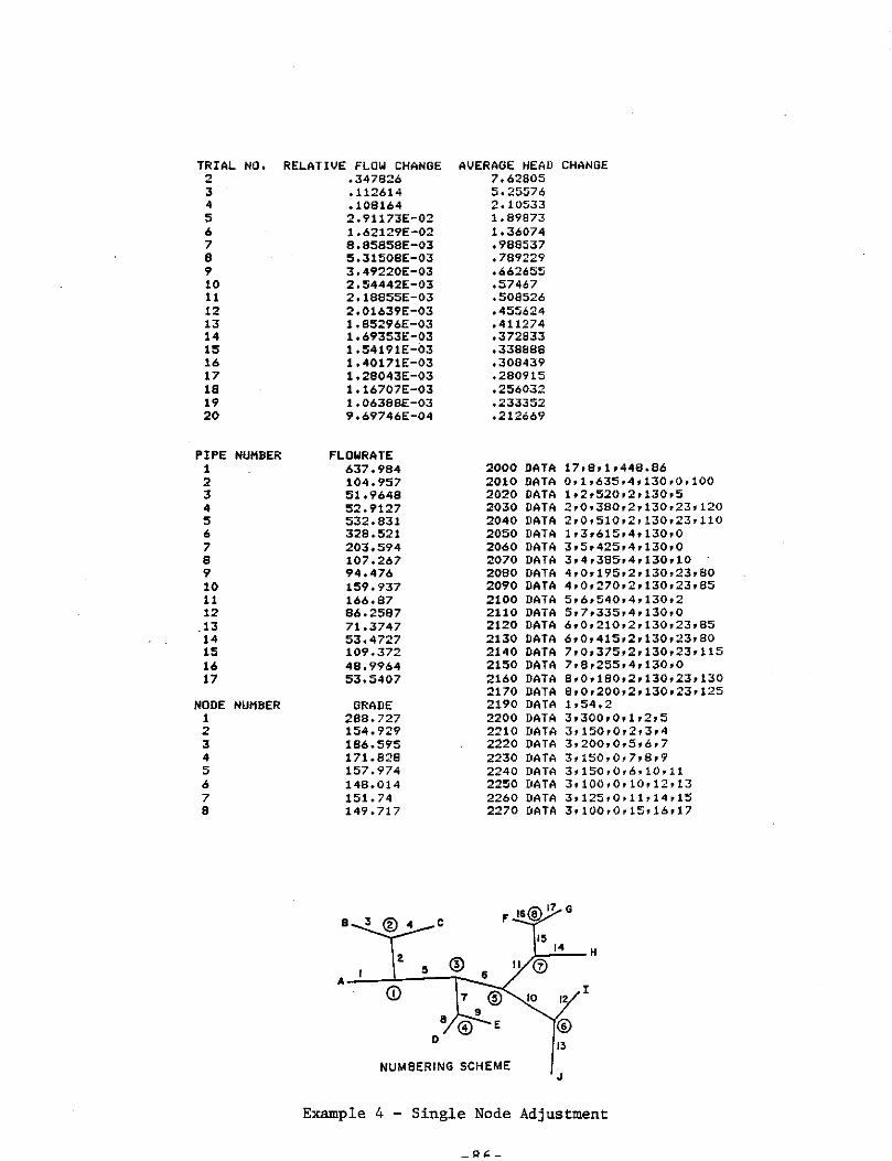
TRIAL NO, RELATIVE FLOW CHANGE AVERAGE HEAD CHANGE 2 .347826 7,62805 3 .112614 5.25576 4 , 108164 2.10533 5 2,91173E-02 1, 89873 6 1.62129E-02 1,36074 7 8,85858E-03 ,988537 8 5,31508E-03 • 789229 9 3,49220E-03 .662655 10 2,54442E-03 ,57467 11 2, 18855E-03 ,508:526 12 2,01639E-03 ,455624 13 1.85296E-03 ,411274 14 1,69353E-03 ,372833 15 1,54191£-03 ,338888 16 1,40171E-03 ,308439 17 1,28043E-03 ,280915 18 l,16707E-03 ,256032 19 1,06388E-03 ,233352 20 9,69746E-04 ,212669
PIPE NUMBER FLOWRATE 1 637,984 2000 DATA 17,8,1,448,86 2 104,957 -2010 DATA 0,1,635,4,130,0,100 3 51,9648 2020 DATA 1,2,520,2,130,5 4 52,9127 2030 DATA 2,0,380,2,130,23,120 5 532,831 2040 DATA 2,0,510,2,130,23,110 6 328,521 2050 [1ATA 1,3,615,4,130,0 7 203,594 2060 DATA 3,5,425,4,130,0 8 107,267 2070 DATA 3,4,385,4,130,10 9 94,476 2080 DATA 4,0,195,2,130,23,80 10 159,937 2090 DATA 4;0,270,2,130,23,85 11 166,87 2100 DATA 5,6,540,4,130,2 12 86,2587 2110 DATA 5,7,335,4,130,0 13 71,3747 2120 DATA 6,0,210,2,130,23,85 14 53,4727 2130 DATA 6,0,415,2,130,23,80 15 109,372 2140 DATA 7,0,375,2,130,23,115 16 48,9964 2150 DATA 7,B,255,4,130,0 17 53,5407 2160 DATA a,o,1ao,2,1Jo,23,130
2170 DATA a,o,200,2,130,23,12s NODE NUMBER BRADE 2190 DATA 1,54.2
1 288.727 2200 DATA 3,300,0,1,2,5 2 154.929 2210 DATA 3,150,0,2,3,4 3 196.595 2220 DATA 3,200,0,5,6,7 4 171.828 2230 DATA 3,150,0,7,8,9 5 157,974 2240 DATA 3,150,0,6,10,11 6 148,014 2250 DATA 3, 100,0, 10, 12, 13 7 151. 74 2260 DATA 3,125,0,11,14,15 8 149,717 2270 DATA 3, 100,0, 15, 10, 17
B 3 @4 c F
2 H
s @ 6
A <D I
7 12
a E © D
13
NUMBERING SCHEME J
Example 4 - Single Node Adjustment
_Q,:._
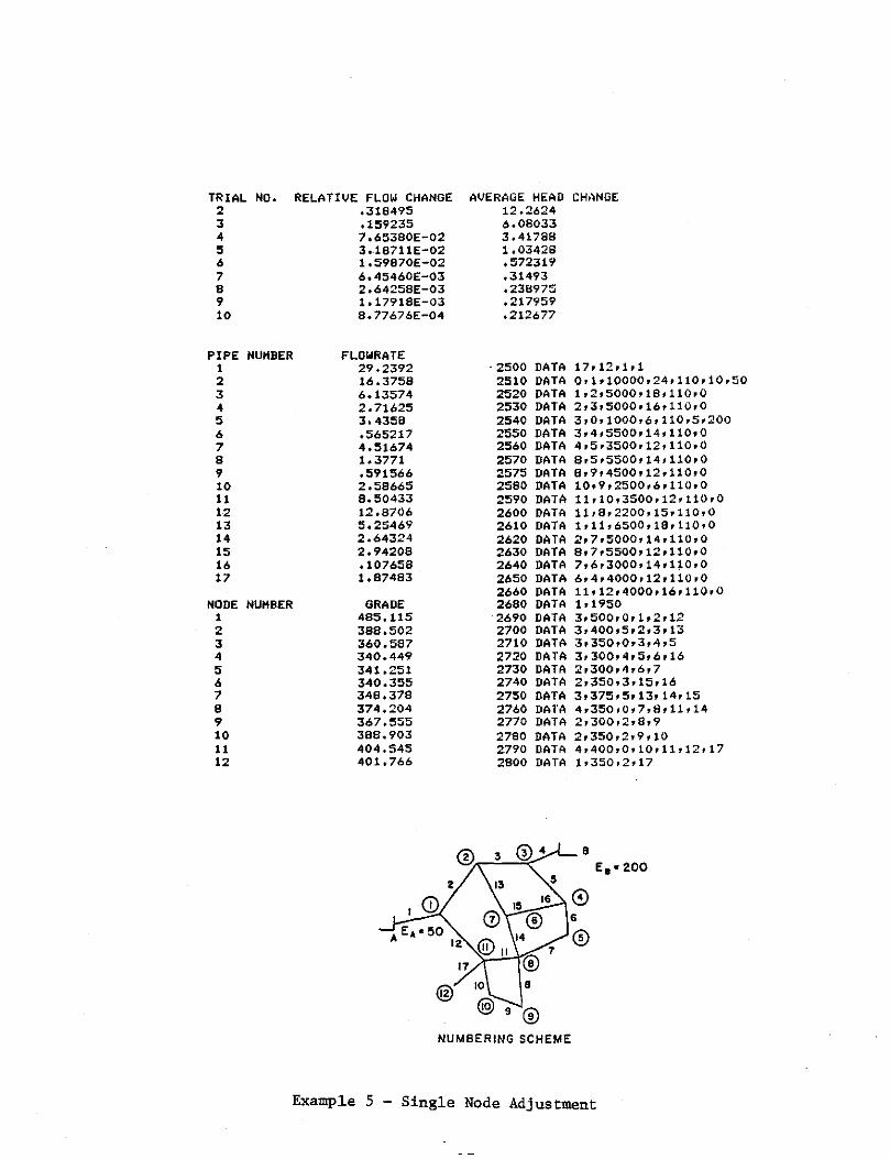
TRIAL NO. 2 3 4 5 6 7 8 9 10
PIPE NUHBER 1 2 3 4 5 6 7 8 9 10 11 12 13 14 15 16 17
NODE NUHBER 1 2 3 4 5 0 7 8 9 10 11 12
RELATIVE FLOW CHANGE AVERAGE HEAD .318495 12.2624 .159235 6.08033 7o65380E-02 3.41788 3.18711E-02 1.03428 1,59870E-02 ,572319 6,45460E-03 ,31493 2,64258E-03 .238975 1,17918E-03 .217959 8,77676E-04 .212677
FLOWRATE 29.2392 · 2500 DATA 16,3758 2510 DATA 6.13574 2520 DATA 2.71625 2530 DATA 3,4358 2540 DATA .565217 2550 DATA 4,51674 2560 DATA 1,3771 2570 DATA ,591566 2575 DATA 2.58665 2580 DATA B,50433 2590 DATA 12.8706 2600 DATA 5.25469 2610 DATA 2.64324 2620 DATA 2,94208 2630 DATA ,107658 2640 DATA t.87483 2650 DATA
26o0 DATA GRADE 2680 DATA
485.115 2o90 DATA 388.502 2700 DATA 300,587 2710 DATA 340,449 2720 DATA 341.251 2730 DATA 340,355 2740 DATA 348,378 2750 DATA 374.204 27o0 DATA 367.555 2770 DATA 388,903 2780 DATA 404.545 2790 DATA 401,760 2800 DATA
9® NUMBERING SCHEME
CH,'tNGE
17,12,1,1 o,1,10000,24,110,10,~o 1,2,5000,18,110,0 2,3,5000,16,110,0 3,0,1000,6,110,5,200 3,4,5500,14,110,0 4,5,3500,12,110,0 8,5,5500,14,110,0 8,9,4500,12,110,0 10,9,2500,0,110,0 11,10,3500,12,110,0 11,a,2200,1s,110,o 1,11,6500,18,110,0 2,7,S000,14,110,0 8,7,5500,12,110,0 7,6,3000,14,110,0 6,4,4000,12,110,0 11,12,4000,16,110,0 1,1950 3,500,0,1,2,12 3,400,5,2,3,13 3,350,0,3,4,5 3,300,4,5,6,16 2,300,4,6,7 2,350,3,15,16 3,375,5,13,14,15 4,350,0,7,8,11,14 2,300,2,8,9 2,350,2,9,10 4,400,0,10,11,12,17 t,350,2,17
a
Example 5 - Single Node Adjustment

TRIAL NO, 2 3 4 5 6 7 a 9
PIPE NUHBER 1 2 3 4 5 6 7 8 9 10 11 12
NODE NUHBER 1 2 3 4 5 6 7 8
RELATIVE FLOW CHANGE .235817 .287243 .109522 4,60690E-02 1.82453E-02 6,27008E-03 2,06382E-03 8,35856E-04
AVERAGE HEAD CHANGE 2.63599
FLOWRATE 4,32484 3,10138 .905732 ,102327 ,640531 1.64572 1.09048 2,30686 +474756 +190984 1.223 3,74085
GRADE 238,765 233.501 232.706 232.776 233,452 236.892 238,329 234,261
E• • 275.38 A
© 2
II
© a
7
0
1.03603 .250238 6.67058E-02 3,40214E-02 1.17870E-02 1+06792E-02 1,09384£-02
1200 DATA 12,a,o,1 1210 DATA 0,1,1500,10,120,0,275.38 1220 DATA 1,2,400,10,120,0 1230 DATA 2,3,000,10,120,0 1240 DATA 3?4,800,8,120,0 1250 DATA B,4,700,B,t20,0 1260 DATA 1,a,1000,10,120,0 1270 DATA 7,6,.750,10,120,0 1280 DATA 6,S,450,10,120,0 1290 DATA 5,4,550,8,120,0 1300 DATA 2,s,aoo,10,120,0 1310 DATA 1,6,800,10,120,0 1320 DATA 0,7,1450,10,120,0,265.38 1330 DATA 3,240,0,1,2,11 1340 IIATA 3,.230,2,2,3,10 1350 DATA 2,23e,1,3,4 1360 DATA 3,237,1,4,5,9 1370 DATA 3,236,2,8,9,10 1380 DATA 3,235,0,7,8,11 1390 DATA 3,234,1,6,7,12 1400 DATA 2,233,1,5,6
® 3 @
10 4 9 © © 5
6 ® 12
NUMBERING SCHEME
B E 0 •265.38
Example 6 - Single Node Adjustment

Appendix 5 Computer Program for Simultaneous Node Adjustment Method -Node Equations
The programs listing (BASIC) which utilizes the procedure presented on pages 10 to 12 in shown on the next- page. To help clarify the program Equ. 35 is written as
=
where A1, A5, B2, B3 and B4 are program variables which represent the respective summations shown in Equ. 35. The program notation for this program is very similar to notation presented in Appendix 4 for the single node adjustment method. The notations defined in lines 140 through 460 in Appendix 3 are identical and will not be repeated here. Additional pertinent notation along with the line number where it first appears.
310
490
530
590
860
970
980
1010
1020
1030
1040
1050
1060
T(N), T(N+N) - pipe numbers for suction and discharge lines for pump number N
Hl - grade at one end of pipe section
H2 - grade at other end of pipe section
S (NJ - a for pipe N (Equ. 34).
A(N,J3) - linearized equation coefficient for 1b A(N,N) - linearized equation coefficient for H a B(N,l) - constant (right side) for linearized equation
Ll - suction line number for pump
L2 - discharge line number for pump
L3 - upstream node number for suction line
L4 - downstream node number for suction line
LS - upstream node number for discharge line
L6 - downstream node number for discharge line
1160 Bl - B (Equ. 371
1170 B(N3,l) - W(Equ. 38)
For data input the pipes are numbered 1 to P and junction nodes 1 to J noting that a pump requires a separate suction and discharge line and junction nodes must be identified at the suction and discharge sides of the pump. When this is done the data coding is carried out using the same instructions as given in Appendix 4· for the single node adjustment method with one exception which is noted for item 3:
3 pipe number for suction line, pipe number for discharge line, useful pump power - repeat this data for each pump (omit this line if system has no pumps).
-89-
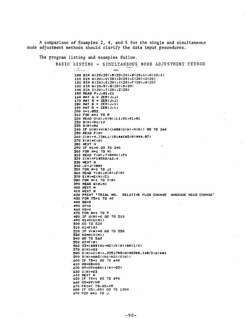
A comparison of Examples 2, 4, and S for the single and simultaneous node adjustment methods should clarify the data input procedures.
The program listing and examples follow. BASIC LISTING - SIMULTANEOUS NODE ADJUSTMENT ~ETHOD
100 DIH A(20,20>,R<20,20>,B<20,1),G(20,1) 110 DIH U<20),V(20),D(20),C(20>,0C20) 120 DIH K<20),E(20),Y(20),F(20>,SC20) 130 DIH WC20,5>,0<20),H<20> 140 DIH I<20),T(20),Z(20) 150 READ P,J,N1,C1 160 HAT A= ZER<J,J) 170 HAT R = ZER<J,J) 180 HAT B = ZERCJ,1) 190 HAT G = ZER<J,ll 200 X=l.852 210 FOR N=I TOP 220 READ U(N),V<N>,Ll,Dl,Rl,Ml 230 D<N>=Dl/12 235 O<N>=Hl 240 IF U<N>+V<N><>ABSCU(Nl-V(Nll GO TO 260 250 READ F<N> 260 C<Nl=4.73*Ll/(Rl**X*D<N>**4•87l 270 K<N>=C<Nl 280 NEXT N 290 IF Nl=O GO TO 340 300 FOR N=l TO NI 310 READ TlN>,T<N+Nll,Pl 320 Z<N>=Pl*550/62,4 330 NEXT N 340 Jl=J-2*N1 350 FOR N=I TO Jl 360 READ Y<N>,H<N>,E<N> 370 E<N>=E<Nl/Cl 380 FOR H=I TO YCN) 390 READ W<N,HJ 400 NEXT 11 410 NEXT N 420 PRINT "TRIAL NO. RELATIVE FLOW CHANGE AVERAGE HEAD CHANGE' 430 FOR T5=1 TO 40 440 08=0 4:0:0 Q5'=0 460 HB=O 470 FOR N=l TOP 480 IF U<Nl=O GO TO 510 490 Hl=H<U(N) l 500 GO TO 520 510 Hl=F<Nl 520 IF V<N>=O GO TO 550 530 H2=H<V(Nl) 540 GO TO 560 550 H2=F<N> 560 03=<ABS<HI-H2l/K<N>l**<1/Xl 570 Q<Nl=03 580 K<N>=C<N>+.02517*0CNl*03**•148/D<Nl**4 590 S<Nl=ABS<<Hl-H2l/K(Nl)
_600 IF T5=1 GO TO 640 610 08=08+03 620 09=09+ABS(I(N)-Q3)
'630 ICNl=03 640 NEXT N 650 IF TS=l GO TO 690 660 05=09/08 670 PRINT T5,0S,H9 680 IF 05<.00I GO TO 1300 690 FDR M=l TO J
-90-

700 FOR H=1 TO J 710 A(N,H)=O 720 NEXT 11 730 NEXT N 740 FOR N=1 TO J1 750 Al=O 760 Bl=O 770 FOR H=1 TO Y(N) 780 L=W<N,11> 790 J3=U(Ll+V<L>-N 800 IF S(Ll=O, GO TO 960 810 AS=S<L>**(l/X-ll/(K(L>*X> 820 A1=A1+A5 830 B2=-<S<L>**(l/Xl> 840 B4=-B2/X 850 IF J3=0 GO TO 920 860 A<N,J3)=A<N,J3)+A5 870 IF H(J3>>H<Nl GO TO 900 880 B2=-B2 890 B4=-B4 900 B1=B1+B2+B4 910 GO TO 960 920 B3=-H(Nl*A5 930 IF F<L>>H<N> GO TO 950 940 B2=-B2 950 B1=B1+B2+B3 960 NEXT 11 970 A<N,N>=-Al 980 B(N,l>=Bl+E(Nl 990 NEXT N 1000 FOR N=l TO Nl .1010 Ll=T <N > 1020 L2=T(N+N1> 1030 L3=U(l1) 1040 L4=V<Ll) 1050 L5=U<L2> 1060 L6=V<L2) 1070 N2=J1+2•N-1 1080 N3=N2+1 1090 IF L3<>0 GD TO 1120 1100 BCN2,1)=-FCL1) 1110 GO TO 1130 1120 A<N2,L3l=l 1130 A<N2,L4>=-1 1140 A(N2,LS>=--KCL1)/K<L2> 1150 A<N2,L6>=K<L1>/K(L2> 1160 B1=Z<Nl/(X*K(L2l*S<L2l**(1/X+1l) 1170 B<N3,ll=Z<N>*<1+1/Xl/S(L2>**(1/X) 1180 A<N3,L4)=-1 1190 A<N3,L5)=1+B1 1200 A<N3,L6)=-B1 1210 NEXT N 1220 HAT R=INV<A) 1230 HAT G =R*B 1240 FOR N=1 TO J 1250 H8=H8+ABS(H(N)-G(N,1)) 1260 H<N>=G(N,1> 1270 NEXT N 1280 H9=H8/J 1290 NEXT TS .1300 PRINT 1310 PRINT 1320 PRINT "PIPE NUMBER FLOWRATE" 1330 FOR N=l TOP 1340 Q(N)=Cl*ABS(O(Nl) 1350 PRINT N,Q(N) 1360 NEXT N 1370 PRINT 1380 PRINT 'NODE NUl1BER GRADE' 1390 FOR N=l TO J 1400 PRINT N,H(Nl 1410 NEXT N
-91-

TRIAL NO, RELATIVE FLOW CHANGE AVERAGE HEAD CHANGE
2 1 6,00331 3 1.2012SE-03 6,05087E-02 4 2.41S63E-05 1,06812E-03
PIPE NUMBER FLOWRATE 1420 DATA 7,2,0,448.86
1 608,558 1430 DATA 0,1,200,4,110,0,188.46
2 95.6236 1440 DATA 1,0,150,2,110,2,86.15
3 448,636 1450 DATA 1,2,200,4,110,0
4 82.16 1460 DATA 2,o,100,2,110,11,64.62
5 64,2971 1470 DATA 1,0,200,2,110,6,100
6 80,5557 1480 DATA 2,0,300,2,110,4,33.08
7 285.918 1490 DATA 2,0,80,4,110,3,B9.23 1520 DATA 4,140,0,1,2,3,5
NODE NUMBER GRADE 1530 DATA 4,100,0,3,4,6,7
1 130.433 2 97,4412
Ea• 86.15 B
C Ee• 64.62
.! 1 '~ NUMBERING
PR l <D 3 ® A D
SCHEME EA•l88.46 .l Eo • 89.23
12 .!i
EF • 100 F E EE •33.08
Example 1 - Simultaneous Node Adjustment
-92-

TRIAL NO. RELATIVE FLOW CHANGE AVERAGE HEAD CHANGE 2 1 87,0873 3 .203535 118,659 4 .307593 73,6377 5 ,184764 31,8814 6 ,159278 11,9253 7 6,16838E-02 8.85837 8 5,08917E-02 3,38077 9 1.77257E-02 ,640245 10 1.13498E-02 .422391 11 7.54545E-03 .292046 12 6,25869E-03 ,21102 13 3,92097E-03 ,154053 14 3,77411E-03 .116092 15 2,13284E-03 8,72378E-02 16 2,47577E-03 6,75436E-02 17 1,16367E-03 5,15275E-02 18 1,73981E-03 4,06568E-02 19 7,39667E-04 3,14178E-02
PIPE NUMBER FLOWRATE 1 9,65661 1800 DATA 15,10,1,1
2 5,27136 1810 DATA 1,2,2000,14,100,8
3 1. 27136 1820 DATA 2,3,3000,14,100,0 4 ,249994 1850 DATA 3,4,2500,14,100,0
5 1.97422 1860 DATA 4,5,2500,14,100,0 6 3,36835 1870 DATA 5,7,2000,14,100,10 7 4,91548 1880 DATA 6,7,1500,12,100,0
8 3,89862 1890 DATA 4,6,2000,14,100,0 9 9,11989 1900 DATA 6,8,3000,14,100,0 10 4,38526 1910 DATA 1,8,2500,14,100,0
11 2.16105 1920 DATA 2,6,2000,14,100,0
12 .605895 1930 DATA 4,o,100,s,100,0,100 13 18.7765 1940 DATA 7,0,200,6,100,10,110
14 3,22128 1950 DATA 10,1,4800,16,100,S 15 18. 7765 1960 DATA 8,0,3200,12,100,0,110
1965 DATA 0,9,200,16,100,0,10 NODE NUMBER GRADE 1970 DATA 15,13,1000
1 202.286 1980 DATA 3,160,0,t,9,13 2 133,299 1990 DATA 3, 120,0,1,2, 10 3 104,528 2000 DATA 2,100,4,2,3 4 102,807 2010 DATA 4,100,4,3,4,7,11 5 102.722 2020 DATA 2,100,2,4,5
6 119,659 2030 DATA 4,110,0,6,7,8,10
7 106,362 2040 DATA 3,105,.2,5,6,12 8 136.114 2050 DATA 3,130,2,S,9,14 9 -.52384 10 468,897
~ EA•IO ~
@O 13 CD ® 2 @ ® 9 10 3
B Ee•IOO II 8 7
®e © 4
Ee• 110 ® Eo•IIO 5
NUMBERING SCHEME
Example 2 - Simultaneous Node Adjustment
-93-

TRrAL NO, RELATIVE FLOW CHANGE AVERAGE HEAD CHANGE 2 1 108,884 3 .775802 130,019 4 , 41116 153.76 5 .281012 127 .139 6 .796696 49,2704 7 .316552 40,2987 8 ,206562 10.051 9 2,86635E-02 1,73391 10 3.23405E-03 , 107019 11 1,25353E-04 3.92456E-03
PIPE NUHBER FLOWRATE 1 635,786 2 105,558 2100 DATA 18,10,1,448.86 3 52,3437 2110 DATA 10,1,535,4,130,0 4 53,2143 2120 DATA 1,2,520,2,130,5 5 530,23 2130 DATA 2,0,380,2,130,23,120 6 325.627 2140 DATA 2,0,510,2,130,23,110 ? 204.602 2150 DATA 1,3,615,4,130,0 8 108,743 2160 DATA 3,5,425,4,130,0 9 95,8605 2170 DATA 3,4,385,4,130,10 10 160,979 2180 DATA 4,0,195,2,130,23,80 11 164,647 2190 DATA 4,0,270,2,130,23,85 12 88,1411 2200 DATA 5,6,540,4,130,2 13 72,8387 2210 DATA 5,7,335,4,130,0 14 55,7038 2220 DATA 6,0,210,2,130,23,85 15 108,944 2230 DATA 6,0,415,2,130,23,80 16 52,4118 2240 DATA 7,0,375,2,130,23,115 17 56,5353 2250 DATA 7,8,255,4,130,0 18 635,785 2260 DATA 8,0,180,2,130,23,130
2270 DATA a,o,200,2,130,23,125 NODE NUHBER GRADE 2275 DATA 0,9,100,4,130,0,100
1 290.641 2290 DATA 18,1,54.2 2 155.371 2300 DATA 3,300,0,1,2,5 3 189.182 2310 DATA 3,150,0,2,J,4 4 174,058 2320 DATA 3,200,0,5,6,7 5 160,76 2330 DATA 3,150,0,7,8,9 6 150,44 2340 DATA 3,150,0,6,10,11 7 154.425 2350 DATA 3, 100, 0, 10, 12, 13 8 152, 18 2360 DATA 3,125,0,11,14,15 9 76,9093 2370 DATA 3,100,0,15,16,17 10 414,177
B 3 @4 c
2 14 H
~Q I ~
@ <D I ® e 9
© E © 0
13
NUMBERING SCHEME J
Example 4 - Simultaneous Node Adjustment
-94-

TRIA.L NO. RELATIVE FLOW CHANGE AVERAGE HEAD CHANGE
2 1 a20.a22 3 .736709 933,51 4 ,289404 . 688.393 5 ,556325 629,608 6 ,267509 169,345 7 .108602 110,453 8 7,04484E-02 14.0286 9 3,27783E-02 4,76694 10 2,75472E-02 3,63112
11 1,59273E-02 2,46052 12 1.61131E-02 1,85413 13 1,01767E-02 1.22515 H 1.17714E-02 .884266 15 7.17961E-03 .466602 16 3.90817E-03 .320872 17' 3.39971E-03 .232746 18 1.70053E-03 .168585 19 2.11461E-03 .126763 20 1.03697E-03 9.2059SE-02 21 1,46189E-03 7,10275E-02 22 7.26101E-04 5.16030E-02
PIPE NUMBER FLOWRATE 1 29,6046 2 16,5054 2500 DATA 18,14,1,1
3 6,15971 2510 DATA 14,1,9900,24,110,10
4 2.60488 25:?0 DATA 1,2,sooo,1s,110,o 5 3,55491 2530 DATA 2,3,5000,10,110,0
6 ,488296 2540 DATA 3,0,1000,6,110,5,200
7 4.48843 2550 DATA 3,4,5500,14,110,0
8 1.41212 2560 DATA 4,5,3500,12,110,0
9 .587806 2570 DATA 9,S,5!500,14,110,0
10 2.58768 2575 DATA B,9,4300,12,110,0
11 8,51142 2580 DATA 10,9,2500,6,110,0
12 13,0994 2590 DATA 11,10,3500,12,110,0 13 5.34551 2600 DATA 11,a,2200,1s,110,o 14 2.6109 2610 DATA 1,11,6500,18,110,0
15 2.95645 2620 DATA 2,7,5000,14,110,0
16 .229796 2630 DATA 8,7,5500,12,110,0
17 1.99969 2640 DATA 7,6,3000,14,110,0
18 29,6045 2650 DATA 6,4,4000,12,110,0 2670 DATA 0,13,100,24,110,0,50
NODE NUMBER GRADE 2680 DATA 18'1'1950
1 474.498 2690 DATA 3,500-,0,1,2,12 2 376.627 2700 DATA 3,.400,5,2,3,13
3 348,638 2710 DATA 3,350,0,3,4,S
4 327,324 2720 DATA 3,300,4,5,6,16
~ 328.052 2730 DATA 2,300,4,0,7
6 327, 118 2740 DATA 2,350,3,15,16
7 335.382 2750 DATA J,,375,5, 13, 14, 15
8 360.877 2760 DATA 4,350,0,7,8,11,14
9 354,194 2770 DATA 2,Joo,2,a,9 10. 375.612 2780 DATA 2,350,2,9,10
11 391.57 2790 DATA 4,400,0,10,11,12,11
12 388,783 28t'O DATA 1,3~0,2,17 13 48.5772 2810 END 14 629.142
8
~O@ A Eol•50
@ 9 ®
NUMBERING SCHEME
Example 5 - Simultaneous Node Adjustment

TRIAL NO. 2 3 4 s 6 7 8 9 10 11
PIPE NUHBER 1 2 3 4 5 6 7 8 9 10 11 12
NODE NUHBER 1 2 3 4 s 6 7 8
RELATIVE FLOW CHANGE 1 .374602 .149486 .178418 7.026SBE-02 ,140007 6,97266E-02 3,56S91E-02 1,20965E-02 5.72392£-04
FLOWRATE 4.2934 3.07665 ,892172 ,107563 ,631397 1,63141 1.07516 2.29106 .476224 .18419 1.21667 3.70666
GRADE 239.25 234,052 233,265 233,327 233,996 237,305 238,775 234.762
E4 • 275.38 A
PR
2
II
© 8
7
0 12
AVERAGE HEAD CHANGE 5,24186 3,65636 2.27042 1.41315 ,070077 .554546 .160944 .121954 4,00423E-02 2.40090E-03
1540 DATA 12,e,o,.1 1550 DATA o,1,1soo,10,120,o,27s.3s 1560 DATA 1,2,400,10,120,0 1570 DATA 2,J,.600,10,120,0 1580 DATA 3,4,800,8,120,0 1590 DATA 8,4,700,8,120,0 1600 DATA 7,8,1000,10,120,0 1610 DATA 7,6,750,10,120,0 1620 DATA 6,S,450•10,120,0 1630 DATA s,4,.530,e,120,o 1640 DATA 2,5,800,10,120,0 1650 DATA 1,o,aoo,.10,120,0 1660 DATA 0,7,1450,10,120,0,265.38 1670 DATA 3,240,0,t ,2, 11 1680 DATA 3,230,2,2,3,10 1690 DATA 2;238,1,3,4 1700 DATA 3r237,1,4,:S,9 1710 DATA 3,236,2,8,9,10 1720 DATA 3,235,0,7,8,11 1730 DATA 3,234,1,6,7,12 1740 DATA 2,233,t,S,6
® 3 @
10 4 9 © © 5
6 ® NUMBERING SCHEME
B E, • 265.38
Example 6 - Simultaneous Node Adjustment
-96-