algorithms for molecular biology biomed central

BioMed CentralAlgorithms for Molecular Biology

ss
Open AcceResearchSMOTIF: efficient structured pattern and profile motif searchYongqiang Zhang and Mohammed J Zaki*
Address: Department of Computer Science, Rensselaer Polytechnic Institute, Troy, New York 12180, USA

Email: Yongqiang Zhang - [email protected]; Mohammed J Zaki* - [email protected]

* Corresponding author

AbstractBackground: A structured motif allows variable length gaps between several components, whereeach component is a simple motif, which allows either no gaps or only fixed length gaps. The motifcan either be represented as a pattern or a profile (also called positional weight matrix). We proposean efficient algorithm, called SMOTIF, to solve the structured motif search problem, i.e., given oneor more sequences and a structured motif, SMOTIF searches the sequences for all occurrences ofthe motif. Potential applications include searching for long terminal repeat (LTR) retrotransposons andcomposite regulatory binding sites in DNA sequences.

Results: SMOTIF can search for both pattern and profile motifs, and it is efficient in terms of bothtime and space; it outperforms SMARTFINDER, a state-of-the-art algorithm for structured motifsearch. Experimental results show that SMOTIF is about 7 times faster and consumes 100 timesless memory than SMARTFINDER. It can effectively search for LTR retrotransposons and is wellsuited to searching for motifs with long range gaps. It is also successful in finding potentialcomposite transcription factor binding sites.

Conclusion: SMOTIF is a useful and efficient tool in searching for structured pattern and profilemotifs. The algorithm is available as open-source at: http://www.cs.rpi.edu/~zaki/software/sMotif/.

BackgroundSearching biological sequence(s) for motifs is a funda-mental task in bioinformatics. Motifs can be representedas either patterns over a specific alphabet, or profiles (alsocalled positional weight matrix (PWM)), which give theprobability of observing each symbol in each position.Motifs can be classified into two main types. If no variablegaps are allowed in the motif, it is called a simple motif. Forexample, in the genome of Saccharomyces cerevisiae, thebinding sites of transcription factor, GAL4 [1], can becharacterized by the simple motif shown in Table 1, whichillustrates the pattern over the IUPAC alphabet (ΣIUPAC;see Table 2), as well as its profile (which gives the fre-quency of each DNA base at each position). The motif in

Table 1 only consists of one component and thus is a sim-ple motif. Since the symbols in the first 3 positions (CGS)and in the last 3 positions (SCG) are well conserved, wecan also represent this motif as CGS[11,11]SCG, where[11,11] means that there is a fixed "gap" of length 11between the two components. If variable gaps are allowedin a motif, it is called a structured motif. A structured motifcan be regarded as an ordered collection of simple motifswith gap constraints between each pair of adjacent simplemotifs. For example, the LTR retrotransposons from theCopia group, corresponding to genes encoding reverse tran-scriptase, in A. thaliana can be characterized by the struc-tured motif M1 [2,5] M2 [6,7] M3, as shown in Table 3[2].Here M1, M2 and M3 are three simple motifs; [2,5] and

Published: 21 November 2006

Algorithms for Molecular Biology 2006, 1:22 doi:10.1186/1748-7188-1-22

Received: 21 May 2006Accepted: 21 November 2006

This article is available from: http://www.almob.org/content/1/1/22

© 2006 Zhang and Zaki; licensee BioMed Central Ltd. This is an Open Access article distributed under the terms of the Creative Commons Attribution License (http://creativecommons.org/licenses/by/2.0), which permits unrestricted use, distribution, and reproduction in any medium, provided the original work is properly cited.

of 24(page number not for citation purposes)

http://www.almob.org/content/1/1/22

http://creativecommons.org/licenses/by/2.0

http://www.ncbi.nlm.nih.gov/entrez/query.fcgi?cmd=Retrieve&db=PubMed&dopt=Abstract&list_uids=17118189

http://www.cs.rpi.edu/~zaki/software/sMotif/

http://www.biomedcentral.com/

http://www.biomedcentral.com/info/about/charter/

Algorithms for Molecular Biology 2006, 1:22 http://www.almob.org/content/1/1/22

[6,7] are variable gap constraints ([minimum gap, maxi-mum gap]) allowed between the adjacent simple motifs.Note that each simple motif Mi (with 1 ≤ i ≤ 3) can eitherbe a pattern over ΣIUPAC or a profile over ΣDNA. Searchingfor structured motifs is more complicated than searchingfor simple motifs, and is an ongoing research area [3-7].The sequence to be searched can be very long, e.g., chro-mosome 1 of Homo Sapiens contains 245 million (245M)base pairs. The structured motif can also be as long as sev-eral kilobases. All these factors need to be consideredwhen designing an efficient structured motif search algo-rithm.

More formally, a structured motif , is specified in theform: M1 [l1, u1] M2 [l2, u2] M3 ... Mk-1 [lk-1, uk-1] Mk,

where Mi, 1 ≤ i ≤ k, is a simple motif component; and li

and ui (with 0 ≤ li ≤ ui), 1 ≤ i <k, are the minimum andmaximum length of the gap allowed between Mi andMi+1, respectively. Note that a gap is defined to be thenumber of intervening positions after Mi but before Mi+1.In other words if si and ei represent the start and end posi-

tions of component Mi, then for i ∈ [1, k - 1], the lengthof the gap between Mi and Mi+1 is given as gi = ei+1 - si -

1, and we require that gi ∈ [li, ui]. We use |Mi| to denotethe number of symbols/positions in component Mi, alsocalled the length of the component, and we use

to denote the total length of the struc-

tured motif (not counting gaps). The maximum span,

L, of the motif is the maximum number of positionsthat can be occupied by the structured motif, which is

given as . The structured motif

can be either specified as a pattern or a profile. When

denotes a pattern, we use the notation j to denote

the symbol at position j in the motif, and when

denotes a profile, we use the notation xj to denote the

frequency of symbol x ∈ ΣDNA at position j, where j ∈ [1,

| |]. Table 3 shows both the pattern and profile repre-sentation of an example structured motif with three com-ponents.

Given a collection of sequences, , over the DNA alpha-

bet ΣDNA = {A,C,G,T}, and a structured motif, , the

structured motif search problem is to report all the occur-

rences (or matches) of in . The occurrence set of the

structured motif, given as , can be reported in twoforms: a) full positions: list of the positions for each symbol

in , for all possible matches in , or b) start positions:

list of the starting positions of for each match in .

Table 4 shows an example sequence and a structured

motif , where M1 = CG, M2 = TTA and M3 = CAT, and

[0, 1] and [1,4] are the intervening gap ranges between M1

and M2, and M2 and M3, respectively. The motif has k = 3

components, it length is | | = 8 and its maximum span

is L = 13. The occurrence set of full positions is ={(5,6,8,9,10,12,13,14), (5,6,8,9,10,15,16,17)}, and of

start positions is = {5}.

Depending on the application, the structured motif searchproblem can have several variations:

• Missing Components: The matching motifs can consist of

some, instead of all, the simple motifs in , allowing forat most q missing components.

• Approximate Matches: The matching motifs may consistof similar motifs (as measured by Hamming or Levenshteindistance [8]), instead of exact matches, to the simple

motifs in , allowing for at most εi errors for simple

motif Mi (when is expressed as a pattern).

• Overlapping Components: The variable gap constraints (liand ui) can take on a limited range of negative values,

| | | | = =∑ iik

1

L M ui iik

ik= + =

−= ∑∑ | |

11

1

Table 1: A Simple Motif

Symbols Motif

A 0 0 0 4 1 1 7 0 5 1 0 2 0 2 0 0 0C 10 0 1 2 3 5 0 7 0 4 2 5 5 1 9 10 0G 0 10 9 4 5 3 2 3 0 3 1 1 4 1 1 0 10T 0 0 0 0 1 1 1 0 5 2 7 2 1 6 0 0 0

IUPAC C G S V N N D S W N B N B N S C G

The binding sites for the transcription factor GAL4 in S. cerevisiae satisfy this motif [1]. Rows 2–5 show the profile (the frequency of observing a DNA base in a given position). The last row shows the corresponding pattern over the IUPAC alphabet.



allowing search for overlapping simple motifs. We allowtwo adjacent components Mi and Mi+1 to overlap, but werequire that Mi+1 does not precede Mi. This condition canbe satisfied by the following constraints on the gap range[li, ui]: - |Mi| ≤ li ≤ ui, for i ∈ [1, k). For example the searchfor motif ACG[-2,2]CGA, can discover the overlappedoccurrence ACGA, as well as the non-overlapped occur-rence ACG- -CGA, at the two extremes of the gap range.

• Profile Search: The components of the motif can be

specified as a pattern in either the DNA (ΣDNA) or IUPAC

(ΣIUPAC) alphabets, or as a profile over ΣDNA.

In this paper, we focus on the problem of searching for agiven structured motif in one or more sequences. We pro-pose SMOTIF, an efficient algorithm for structured motifsearches. It uses an inverted index of symbol positions,and it finds all occurrences by positional joins over thisindex. For structured pattern search problem, we proposetwo main variants of our approach: i) a direct search forsimple motifs and the structured motif via positionaljoins, and ii) a two-step approach, where we use a suffixtree to search for simple motifs and then use positionaljoins for the structured motif. For structured profile searchproblem, we first search each simple motif by aligning itsprofile with the sequences, and then search structuredmotifs with positional joins. SMOTIF allows missing com-ponents, overlapping motifs, and also approximatematches (when using the two-step approach). SMOTIFalso allows flexible matches using IUPAC symbols.

We apply SMOTIF for searching long DNA sequences forLTR retrotransposons, which constitute a substantial frac-tion of most Eukaryotic genomes and are believed to havea significant impact on genome structure and function[9,10]. We show that SMOTIF is effective in searching forcomposite regulatory patterns, and it can also suggestpotentially new binding sites. We experimentally demon-strate the superiority of SMOTIF over SMARTFINDER, astate-of-the-art method for structured motif search, bothin terms of time and space; SMOTIF can be up to 7 timesfaster and can consume 100 times less space.

Related workMany existing pattern matching algorithms [8,11-18] canbe used to solve the simple pattern search problem. Giventhe sequence length, n, and the pattern length, m, exactmatching algorithm can run in O (n + m) [11]; approxi-mate matching algorithm can run in O (rn) [16,17] or O(nm/w) [18], where r is the error threshold and w is thesize of a computer word. The space complexity is O (n) forboth exact matching and approximate matching.

Several previous efforts have focused on the structuredpattern search problem. Anrep [3,4] provides a unifiedbiosequence pattern representation by using networkexpressions with spacers, where a network expression is a reg-ular expression without Kleene closure. With networkexpressions, one can specify the scoring scheme and thethreshold of approximate matching for each simple motifseparately, the positional weights which express the rela-tive importance of different parts of a motif, and whethera simple motif is optional. Anrep introduces a two-stepapproach: first it searches for simple motifs by a thresh-old-sensitive motif matching algorithm and then it findsthe structured motif by an optimized backtracking match-ing algorithm. However, as compared by [6], Anrep ismuch slower than SMARTFINDER.

In [5], the structured motif is called a Classes of Charactersand Bounded Gaps (CBG) expression and is represented by

Table 3: A Structured Motif

Symbols M1 M2 M3

A 2 12 17 1 11 1 35 0 24 1 0 3 1 35C 0 10 8 5 2 0 0 19 0 0 25 5 35 1G 2 5 5 2 10 34 1 0 0 26 11 0 0 0T 32 9 6 28 13 1 0 17 12 9 0 28 0 0

IUPAC D N N N N D R Y W D S H M M

We aligned the 36 A. thaliana LTR retrotransposons from Repbase Update [2] database which belong to Copia group corresponding to genes encoding reverse transcriptase to obtain the structured motif M1 [2,5] M2 [6,7] M3. Rows 2–5 show the profile (the frequency of observing a DNA base in a given position), and the last row shows the corresponding pattern over the IUPAC alphabet.

Table 2: IUPAC Alphabet (ΣIUPAC)

Symbol A C G T U R Y KBases A C G T U A,G C,T G,T

Symbol M S W B D H V NBases A,C G,C A,T C,G,T A,G,T A,C,T A,C,G A,C,G,T



a non-deterministic ε-automaton with bit parallelism.Two algorithms are proposed for CBG expression search:forward search and backward search. Bit parallelismspeeds up the search, but is adequate only for a patternwhose maximum span is smaller than the length of thecomputer word. Also the implementation of CBG canonly handle such pattern. This limits the application ofCBG to searching for patterns with small number of sym-bols and gaps.

SMARTFINDER [6,7], which is currently the most efficientmethod for structured motif search, is also a two-stepapproach. In the first step each simple motif is searchedseparately by building a suffix tree for the sequence. Thisstep outputs the ordered occurrence lists of all simplemotifs. The second step solves a constraint satisfaction prob-lem by considering constraints individually in three sub-steps. First it considers the gap constraints and builds aconstraint graph whose nodes are the simple motif occur-rences and edges connect all possible pairs of nodes thatlocally satisfy the gap constraints. It then considers theconstraint for the maximum number of missing compo-nents and shrinks the graph to contain only the nodes thatcan be in the structured motif occurrences. Finally it enu-merates all the valid occurrences by a depth first search(DFS). Notable differences in SMOTIF and SMART-FINDER are as follows: we search patterns directly by posi-tional joins over an inverted index, we consider variablegap constraints during the positional joins as opposed tobuilding a constraint graph, and we handle missing com-ponents more efficiently by considering them over pat-terns instead of over each occurrence as in SMARTFINDER.Note also that like Anrep and SMARTFINDER, SMOTIFcan also mine approximate patterns, when using the two-step approach, which we describe later.

For profile search, MATCH [19], P-Match [20], and MatIn-spector [21,22] search DNA sequences against a positionweight matrix library (such as TRANSFAC database [23])and report the occurrences that satisfy given score thresh-olds. They compute the matrix score by multiplying thebase frequency with the information content value at eachposition, in order to emphasize the fact that mismatchesat less conserved positions are more easily tolerated thanmismatches at highly conserved positions. Besides the

matrix score, they define a core region, which is usually thefirst 4–5 most conserved consecutive positions of thematrix, and perform the core score threshold check. Thenthey align the matrix to each position of the sequence andcalculate the core score and matrix score. However, thesealgorithm don't consider the prior probability of eachbase when calculating the matrix (or core) score, and thecore region is required to be consecutive. They need tocheck all positions of each subsequence (at least all thecore positions) in order to calculate the matrix (core)score. Moreover, these algorithms only work on simpleprofile with one single matrix component. For structuredprofile search, only Anrep [3,4] provides the capability tomodel structured profiles, with its general network expres-sions. However, Anrep doesn't give a solution on scorecalculation and fast search for structured profiles. Moreo-ver, its implementation doesn't support structured profilesearch. To our knowledge, SMOTIF is the only imple-mented method that can handle structured profile search.

MethodsWe first introduce our basic approach for structured pat-tern search, and successively optimize it for various prac-tical scenarios. We then present our approach forstructured profile search.

Structured pattern search: basic approach

Let us assume that we are searching for a structured motif

over a single sequence S ∈ . We assume that S is

over ΣDNA, whereas, is over ΣIUPAC to allow for more

flexible matches. SMOTIF first converts S into an equiva-lent inverted format [24,25], where we associate with eachsymbol in the sequence its pos-list, a sorted list of the posi-tions where the symbol occurs in S. More formally, for a

symbol X ∈ ΣIUPAC, its pos-list is given as (X, S) = {i | S

[i] = X, i ∈ [1, |S|]}, where S [i] is the symbol at position iin S, and |S| denotes the length of S. When S is obvious,we drop it, and denote the pos-list as (X). For our

example sequence S in Table 4, the pos-lists for X ∈ ΣDNA

are given in Table 5.

Depending on whether we compute the pos-lists forIUPAC symbols or not, SMOTIF uses two approaches: (a)DNA pos-lists: Here we keep (in memory) the pos-lists onlyfor the four DNA symbols. For the other IUPAC symbols,we obtain their pos-lists by taking a union over the pos-lists of their constituting DNA symbols, e.g., (R) =

(A) ∪ (G) = {1, 3, 5, 7, 10, 11, 13, 16}. (b) IUPACpos-lists: Here we keep (in memory) the pos-lists for the

IUPAC symbols that actually appear in . These pos-lists are computed directly by scanning S once.

Table 4: Structured Motif Search

Sequence (S ∈ ): GCATGCGTTAGCATCATC

Structured Motif ( ): GC[0,1]TTA[1,4]CAT

Occurrences of in are marked in bold.



Positional joins

We first extend the notion of pos-lists to cover structured

motifs. The pos-list of is given as the set of start posi-

tions of all the matches of in S. Let X, Y ∈ ΣIUPAC be

any two symbols, and let = X [l, u] Y be a structured

motif. Given the pos-lists of X and Y, namely, (X) and

(Y), the pos-list for can be obtained by a positional

join as follows: For a position x ∈ (X), if there exists a

position y ∈ (Y), such that l ≤ y - x - 1 ≤ u, it means thatY follows X within the variable gap range [l, u] in thesequence S, and thus we can add x to the pos-list of motif

X [l, u] Y. Let d be the length of the gap between x ∈ (X)

and y ∈ (Y), given as d = y - x - 1. Then, in general, thereare three cases to consider in the positional join algo-rithm, as shown in Figure 1,

• d <l: Advance y to the next element in (Y).

• d > u: Advance x to the next element in (X).

• l ≤ d ≤ u: Save this occurrence in (X [l, u] Y), and thenadvance x.

The pos-list for X [l, u] Y can be computed in time linearin the lengths of (X) and (Y). In essence, each time

we advance x ∈ (X), we check if there exists a y ∈ (Y)that satisfies the given gap constraint. Instead of searchingfor the matching y from the beginning of the pos-list eachtime, we search from the last position used to comparewith x. This results in fast positional joins, and also allowsoverlaps among occurrences. For example, during thepositional join for the motif T[0, 1]A, with l = 0 and u = 1,we scan the pos-lists of T and A in Table 5. Initially, x = 4and y = 3. This gives d = 3 - 4 - 1 = -2 <l, thus we advancey to 10. Next, d = 10 - 4 - 1 = 5 > u, thus we advance x to 8.

Next, d = 10 - 8 - 1 = 1 ∈ [0, 1]. So we store x = 8 in (T[0,1] A) and advance x to 9. By continuing the process, we getthe final pos-list as (T[0,l] A) = {8, 9, 14}.

Given a longer motif , the positional joins start withthe last two symbols, and proceed by successively joiningthe pos-list of the current symbol with the intermediatepos-list of the suffix. Formally, let H [l, u] T be an interme-diate pattern, with symbol H as the head symbol, and a suf-fix structured motif T as tail. The pos-list of H [l, u] T isobtained by doing positional join on the pos-list of H andthe pos-list of T. As the computation progresses the previ-ous tail pos-lists are discarded. Combined with the factthat only start positions are kept in a pos-list, this savesboth time and space.

SMOTIF handles both simple and structured motifs uni-formly, by adding the gap range [0, 0] between adjacentsymbols within each simple motif Mi. For our example in

Table 4, the structured motif becomes:G[0,0]C[0,1]T[0,0]T[0,0]A[1,4]C[0,0]A[0,0]T. Further-more, SMOTIF treats the IUPAC symbol N (which standsfor any of the four bases: A,C,G,T) as a gap, [1,1], andmerges it with adjacent gaps in the motif. For example, themotif A[0,0]N[0,0]N[0,0]C will be first converted to A[0,0][1,1][0,0][1,1][0,0]C, and then the adjacent gaps will becombined to obtain A[2,2]C as the final motif.

Figure 2 shows how the positional joins work for our(expanded) motif from Table 4. At any stage in the proc-ess, the head symbol's pos-list corresponds to the full listof positions shown, whereas the tail's pos-list consistsonly of the positions shown in bold. For example, whencomputing A[1,4]CAT, the pos-list of the tail CAT is {2,12, 15}, and that of the head symbol A is {3, 10, 13, 16}.Also, for illustration, we add a link between any two posi-

Positional Joins AlgorithmFigure 1Positional Joins Algorithm.

Positional-Joins(P(X),P(Y ), l, u)1 i← j ← k ← 1;2 while (i ≤ |P(X)| and j ≤ |P(Y )|) do3 d← P(Y )[j]− P(X)[i]− 1;4 if (d < l) then5 j ← j + 1;6 else if (d > u) then7 i← i + 1;8 else9 P(X [l, u]Y )[k]← i;

10 i← i + 1;11 k ← k + 1;

12 return P(X [l, u]Y );

Table 5: Pos-lists

A C G T

3 2 1 410 6 5 813 12 7 916 15 11 14

18 17



tions (x and y) in adjacent columns if their difference (d =y - x - 1) falls within the corresponding gap range. Thejoins begin with the last two symbols, with A as the headand T as the tail with a gap of [0,0]. The only positions x

∈ (A) that satisfy the adjacent gap constraint are 3, 13and 16 (marked in bold), that form the pos-list of A[0,0]T.Next we join (C) with (A[0,0] T) to get the validpositions 2,12 and 15. At the next step we need to con-sider A as the head, with constraint [1,4], followed by thetail C [0,0] A [0,0] T. The only positions in (A) that sat-isfy the gap constraint of l = 1 and u = 4 are 10 and 13.Note also how position 2 that was in the tail's pos-list can-not be extended, since there is no position where A occurswithin a gap of [1,4] before the tail CAT. The join processcontinues until the first symbol, and we finally get 5 as theonly start occurrence for the full structured motif.

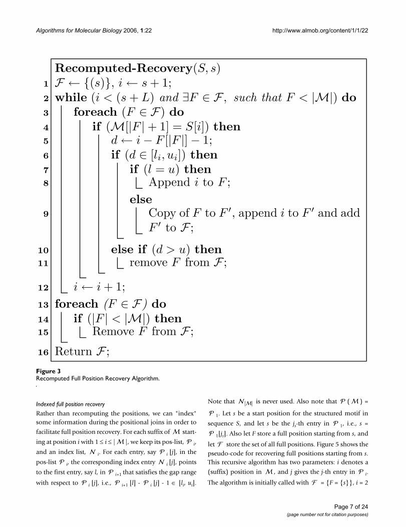
Full position recoveryIn our positional join approach, to save time and space weretain only the motif start positions, however, in someapplications, we may need to know the full position ofeach occurrence, i.e., the set of matching positions foreach symbol in the motif. We describe two approaches torecover the full positions: recomputed or indexed full-position recovery.

Recomputed full position recovery

For recomputing the full positions SMOTIF needs access

to only the sequence S and the post-list ( ). Let s ∈

( ) be a start position for the structured motif insequence S. Figure 3 shows how to recompute the fullpositions starting from s. Note that a structured motif withmaximum span L must be found within position range [s,s + L - 1], so we can stop searching from s after the maxi-

mum span is reached. During the full position recovery,

we maintain a list of intermediate position prefixes

that match the prefix of . For an intermediate prefix F

∈ , let |F| denote the number of positions in F. Initially

= {(s)}. For each symbol S [i] with i ∈ [s + 1, s + L - 1]

in sequence S, we consider each candidate prefix F ∈

and check whether [|F| + 1] = S [i] and d = i - F [|F|] ∈

[l, u]. If yes, S [i] is a valid occurrence of [|F| + 1], andwe append position i to F. If there are multiple positions i

that are valid occurrences for [|F| + 1], we add as many

copies of F appended with the i positions to . A prefixF is removed if there are no symbols in S which matchwithin the maximum gap. The algorithm stops once all F

∈ are full positions or if the maximum span L has beenreached.

As an example, let's assume we want to recover the full

position for the motif = GC[1,2]T in our the sequenceS from Table 4, starting from position s = 5. The recoveryprocess is illustrated in Figure 4. Since the maximum span

of is L = 5 the figure shows positions 5 through 9 in S,

which are the only valid positions where may be

found. Initially, = {(5)}, and we know that [1] = S

[5]. Next S [6] = C = [2] match and are also adjacent in

S, so we update = {(5, 6)}. We discard S [7] since it

doesn't match [3]. However, both S [8] = T = [3]

and S [9] = T = [3] are valid matches within the gap

constraints. Thus we update = {(5, 6, 8), (5, 6, 9)}. Atthis point we have reached the maximum span, and also

all F ∈ are full positions, so we stop.

Positional Joins ExampleFigure 2Positional Joins Example. The figure shows how the positional joins work for the (expanded) motif from Table 4.

[0, 0][0, 0][1, 4]

10139

867

G [0, 0] C [0, 1] T [0, 0] T [0, 0] A C A

1

11

2

1518

12

17 17

4

914

48

14

3

16

6

18

10 89

2 3 4

1215

13141617

5

T



Indexed full position recovery

Rather than recomputing the positions, we can "index"some information during the positional joins in order to

facilitate full position recovery. For each suffix of start-

ing at position i with 1 ≤ i ≤ | |, we keep its pos-list, i,

and an index list, i. For each entry, say i [j], in the

pos-list i, the corresponding index entry i [j], points

to the first entry, say l, in i+1 that satisfies the gap range

with respect to i [j], i.e., i+1 [l] - i [j] - 1 ∈ [li, ui].

Note that is never used. Also note that ( ) =

1. Let s be a start position for the structured motif in

sequence S, and let s be the js-th entry in 1, i.e., s =

1[js]. Also let F store a full position starting from s, and

let store the set of all full positions. Figure 5 shows thepseudo-code for recovering full positions starting from s.This recursive algorithm has two parameters: i denotes a

(suffix) position in , and j gives the j-th entry in i.

The algorithm is initially called with = {F = {s}}, i = 2

| |

Recomputed Full Position Recovery AlgorithmFigure 3Recomputed Full Position Recovery Algorithm.

Recomputed-Recovery(S, s)1 F ← {(s)}, i← s + 1;2 while (i < (s + L) and ∃F ∈ F , such that F < |M|) do3 foreach (F ∈ F) do4 if (M[|F |+ 1] = S[i]) then5 d← i− F [|F |]− 1;6 if (d ∈ [li, ui]) then7 if (l = u) then8 Append i to F ;

else9 Copy of F to F ′, append i to F ′ and add

F ′ to F ;

10 else if (d > u) then11 remove F from F ;

12 i← i + 1;13 foreach (F ∈ F) do14 if (|F | < |M|) then15 Remove F from F ;

16 Return F ;



and with j = 1[js]. Since we have 2[j] - F [1] - 1 ∈ [l1,

u1] we set F [2] = 2[j]. In the next call we can follow the

index 2[j] to get the next position in F, namely F [3].

Thus in each call we keep following the indices from onepos-list to the next and finally we can get a full position

starting from s when we reach the last pos-list, . Fur-

thermore, at each suffix position i, since j only marks thefirst position in i+1 that satisfies the gap constraints, we

also need to consider all the subsequent positions j' > jthat may satisfy the corresponding gap range.

Consider the example shown in Figure 6 to recover the fullpositions for our example motif from Table 4. Under eachsymbol we show two columns. The left column corre-sponds to the intermediate pos-lists i (compare to Fig-

ure 2), whereas the right column stores the indices i

into the pos-list i+1. For example, (A[0,0]T) = 7 =

{3, 13, 16}, and 7 = {1, 4, 5}. For example, for entry

7[2] = 13, we have 7[2] = 4, which means that the

first position in 8 = (T) that satisfies the gap range

[0,0] is 14, which occurs at index 4, i.e., 8[4] - 7[2] -

1 = 14 - 13 - 1 = 0 ∈ [0,0]. To recover the full position forour example motif, from start position 5, we follow index

1 to get position 6 in the next pos-list, to obtain = {(5,

6)}. Then we keep following the indices and get = {(5,6, 8, 9)}. In the next step, we follow to position 10 (atindex 1); a quick check for the gap range [0,0] discards

position 13. We now have = {(5, 6, 8, 9, 10)}. In thenext step we immediately jump to position 12 (at index2). However, both 12 and 15 are within the gap range[1,4]. From 12, we will eventually get F = (5, 6, 8, 9, 10,12, 13, 14), whereas from 15, we will eventually get F = (5,6, 8, 9, 10, 15, 16, 17), as the two possible full-positions.

Sequence segmentation

The SMOTIF approach as described above works well forsearching a motif in a relatively short sequence. For a verylong sequence S (e.g., searching for (LTR) retrotransposonsin an entire chromosome) the pos-lists can get very longin the initial stages, consuming a lot of memory. SMOTIFhandles a long sequence by splitting it into several seg-ments and searches each segment separately for the struc-tured motif. That is, the sequence S is split into p equalpartitions (except for the last one). Handling each smaller

segment Si (i ∈ [l, p]) instead of the original S can save a

lot of space and also reduces the total search time. Aftersegmentation, to avoid missing any occurrence, we

require that each partition Si, with i ∈ [l, p - 1], include the

| |

Indexed Full Position Recovery AlgorithmFigure 5Indexed Full Position Recovery Algorithm.

Indexed-Recovery(i, j, F )1 if (i > |M|) then2 Add F to F ;3 foreach (|Pi| ≥ j′ ≥ j such that (Pi[j′]− F [i− 1]− 1) ∈ [li, ui]) do4 F [i]← Pi[j′];5 Indexed-Recovery(i + 1, Ni[j′], F );6 if (i=2) then7 Return F ;

Recomputed Full-position Recovery ExampleFigure 4Recomputed Full-position Recovery Example. The fig-ure shows how recomputed full-position recovery, using the structured example shown.

Full−positions

PositionSymbol

5G

6 7 8 9C G T T

G[0,0]C[1, 2]T

(5, 6, 8) (5, 6, 9)

Structured Motif



first L - 1 symbols from partition Si+1. Finally, to avoid

duplicate occurrences, we discard all occurrences with astart position in the overlap region, since it would bereported when we process segment Si+1. For example, let S

be the sequence in Table 6, and let the structured motif be

= GC[1,2]T with maximum span L = 5. If p = 3, thenwe would have three segments of length 6 each. After add-ing the overlap region of L - 1 = 4 positions at the end ofeach segment, we obtain the final three segments shown

in Table 6. Two start positions of would be found inS1 (namely 1 and 5), and one in S2 (namely 11). Note that

start positions 5 and 11 would have been missed if we hadno overlap.

So far we have assumed that we are searching for the struc-tured motif in a single sequence. SMOTIF can easily han-

dle a collection of sequences. We simply search eachsequence separately using segmentation when necessary.

Missing components

In some applications a partial match of the structuredmotif might still be of interest. SMOTIF allows up to qsimple motif components to be missing during the search.

Let be a structured motif with k components. SMOTIFfirst enumerates all possible sub-motifs having k' compo-

nents, where k' ∈ [k - q, k]. Next, the gap ranges areadjusted in each sub-motif to account for skipping overthe missing components. The new gap range, [li,j, ui,j],

between components Mi and Mj (with 1 ≤ i <j ≤ k) in a sub-

motif, is calculated as follows: , and

.

For example, if we allow one (q = 1) missing componentfor our structured motif in Table 4, the set of sub-motifsthat need to be searched for are: GC[0,1]TTA[1,4]CAT,GC[1,8]CAT, GC[0,1]TTA and TTA[1,4]CAT. Note that itis straightforward to incorporate other approaches tocompute new ranges into SMOTIF since it would onlychange the gap constraints. For example, li,j = minn ∈ [i,j-1]{ln} and ui,j = maxn ∈ [i,j-1] {un} is another possible way tocompute the adjusted gap ranges.

Instead of searching each sub-motif separately, we do anoptimized search. We reuse the partial pos-lists createdwhen using a depth first search to enumerate and searchthe sub-motifs. The idea is to re-use the pos-lists createdfor common suffixes when enumerating their sub-motifextensions.

Two-step approach for structured pattern search

So far we have described the direct method used by SMO-TIF to search for the structured motif by positional joinsover the symbols. In fact, SMOTIF, can also follow a two-step approach like in Anrep [4] and SMARTFINDER [6]. In

the first step, given and , we search for each sim-

ple motif in , i.e., M1, M2, ..., Mk. This task can be

solved by existing pattern matching algorithms. In the sec-ond step, we do positional joins on the pos-lists of thesimple motifs. Let (Mi [li, ui] ) be an intermediate

l li j nnj

, = =−∑ 11

u u u Mi j i n nn ij

, ( | |)= + += +−∑ 11

Table 6: Segmentation into p = 3

S G C A T G C G T T A G C A T C A T CS1 G C A T G C G T T AS2 G T T A G C A T C AS3 A T C A T C

Indexed Full-position Recovery ExampleFigure 6Indexed Full-position Recovery Example. The figure shows how indexed full-position recovery, using the (expanded) motif from Table 4.

13

G [0, 0] C [0, 1] T [0, 0] T [0, 0] A A[1, 4] [0, 0] [0, 0] TC5 6 8 9 10 3

3131512 2

41 1 1 1

16

1 −2 2 1

3−

17

89

−−

−514

4



pos-list, with simple motif Mi as the head, and a suffix

structured motif = Mi+1 � Mk as tail. Since (Mi)

stores only the start positions, we need convert them intoend positions to check the gap constraints. There are twocases to consider.

Exact matching

Many algorithms [11-14] exist for exact pattern matching.Like in SMARTFINDER we use a lazy suffix tree [11] toextract the pos-lists for all simple motifs. The matchingoccurrences are sorted after extracting them from the suf-fix tree to obtain the pos-list in sorted order. For an inter-

mediate pattern Mi [li, ui] , each start position s ∈ (Mi

[li, ui] ) is converted into an end position s + |Mi| - 1.

Figure 7(a) shows an example of the pos-list join usingexact matches for simple motifs. Each column shows thepos-list for a simple motif in the structured motif fromTable 4. We first join the pos-lists of TTA and CAT, check-

ing for gap range [1,4]. The start position 8 ∈ (TTA) isconverted to end position 8 + 3 - 1 = 10. We find that bothpositions 12 and 15 lie within the minimum and maxi-mum gap range (indicated by the links), and thus 8 isretained in the resulting pos-list. Likewise 5 is in the finalpos-list, since after obtaining its end position 5 + 2 - 1 = 6,

we find d = 8 - 6 - 1 = 1 ∈ [0, 1].

Approximate matchingSeveral algorithms [8, 12, 15–18] exist for approximatepattern matching. For consistency, we used Sellers'dynamic programming algorithm [26], as implementedin SMARTFINDER, to extract the pos-lists for all simplemotifs with approximate matches. This algorithm is notoptimal and it can be replaced by more efficient ones [16-

18]. Since we allow a specific Levenshtein distance [8](i.e., insertions, deletions and substitutions) between theoccurrences and the motif, the length of the occurrencescan be different from the component length |Mi|. Thus weaugment the pos-list to explicitly store the end position, inaddition to the start position, for each occurrence. Figure7(b) shows how the pos-list joins work for approximatematches of simple motifs. In the structured motif fromTable 4, we consider the exact matches of GC and CAT,and the approximate matches of TTA within Levenshteindistance of 1. Each column in (b) shows the pos-list of asimple motif: the left sub-column is a list of its start posi-tions and the right sub-column is a list of its end posi-tions. We first join the pos-lists of TTA and CAT, checkingfor gap range [1,4]. We compare the end positions of TTAand the start positions of CAT and find that the pairs(9,12), (10,12), (10,15), and (11,15) all lie within the gaprange (indicated by the links), and thus the pairs, (7, 10),(8, 9), (8, 10) and (8, 11) are retained in the resulting pos-list. Likewise (5, 6) is in the final pos-list, since after com-paring the end position of GC, 6, with the start position ofTTA, 7 and 8, we find d = 7 - 6 - 1 = 0 ∈ [0,1] and d = 8 - 6- 1 = 1 ∈ [0, 1].

Structured profile search

Having outlined our approach for structured patternsearch, here we tackle the problem of structured profilesearch. The profile (also called a position weight matrix)

for a structured motif gives for each position in eachcomponent, the frequency of occurrence for each symbol

in ΣDNA, i.e., xj gives how often symbol x ∈ ΣDNA occurs

at position j. Note that, as in the case of pattern motifs, for

a structured profile motif , we have to specify the gapconstraints between its simple profile motif components.Profiles are able to better capture the variability in the

Simple Motif Positional Joins ExampleFigure 7Simple Motif Positional Joins Example. The figure shows an example of positional joins on simple motifs, using the motif from Table 4.

16

[0, 1]

10

[1, 4]

91511

8 21215

14

[0, 1]

8

[1, 4]

71511

2612

21215

4

17148

811

(b)(a)

10GCCATTTAGC TTA CAT



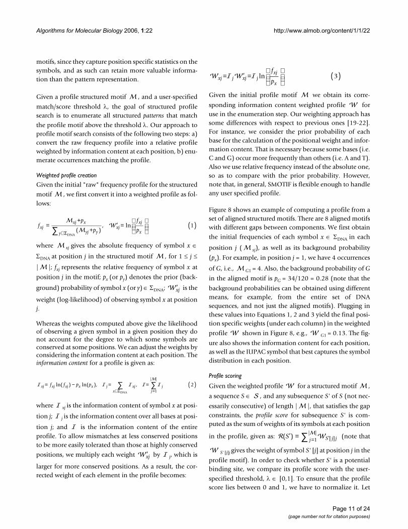
motifs, since they capture position specific statistics on thesymbols, and as such can retain more valuable informa-tion than the pattern representation.

Given a profile structured motif , and a user-specified

match/score threshold λ, the goal of structured profilesearch is to enumerate all structured patterns that match

the profile motif above the threshold λ. Our approach toprofile motif search consists of the following two steps: a)convert the raw frequency profile into a relative profileweighted by information content at each position, b) enu-merate occurrences matching the profile.

Weighted profile creation

Given the initial "raw" frequency profile for the structured

motif , we first convert it into a weighted profile as fol-lows:

where xj gives the absolute frequency of symbol x ∈

ΣDNA at position j in the structured motif , for 1 ≤ j ≤

| |; fxj represents the relative frequency of symbol x at

position j in the motif; px (or py) denotes the prior (back-

ground) probability of symbol x (or y) ∈ ΣDNA; is the

weight (log-likelihood) of observing symbol x at positionj.

Whereas the weights computed above give the likelihoodof observing a given symbol in a given position they donot account for the degree to which some symbols areconserved at some positions. We can adjust the weights byconsidering the information content at each position. Theinformation content for a profile is given as:

where xj is the information content of symbol x at posi-

tion j; j is the information content over all bases at posi-

tion j; and is the information content of the entireprofile. To allow mismatches at less conserved positionsto be more easily tolerated than those at highly conserved

positions, we multiply each weight by j, which is

larger for more conserved positions. As a result, the cor-rected weight of each element in the profile becomes:

Given the initial profile motif we obtain its corre-

sponding information content weighted profile foruse in the enumeration step. Our weighting approach hassome differences with respect to previous ones [19-22].For instance, we consider the prior probability of eachbase for the calculation of the positional weight and infor-mation content. That is necessary because some bases (i.e.C and G) occur more frequently than others (i.e. A and T).Also we use relative frequency instead of the absolute one,so as to compare with the prior probability. However,note that, in general, SMOTIF is flexible enough to handleany user specified profile.

Figure 8 shows an example of computing a profile from aset of aligned structured motifs. There are 8 aligned motifswith different gaps between components. We first obtain

the initial frequencies of each symbol x ∈ ΣDNA in each

position j ( xj), as well as its background probability

(px). For example, in position j = 1, we have 4 occurrences

of G, i.e., G1 = 4. Also, the background probability of G

in the aligned motif is pG = 34/120 = 0.28 (note that the

background probabilities can be obtained using differentmeans, for example, from the entire set of DNAsequences, and not just the aligned motifs). Plugging inthese values into Equations 1, 2 and 3 yield the final posi-tion specific weights (under each column) in the weighted

profile shown in Figure 8, e.g., G1 = 0.13. The fig-

ure also shows the information content for each position,as well as the IUPAC symbol that best captures the symboldistribution in each position.

Profile scoring

Given the weighted profile for a structured motif ,

a sequence S ∈ , and any subsequence S' of S (not nec-

essarily consecutive) of length | |, that satisfies the gapconstraints, the profile score for subsequence S' is com-puted as the sum of weights of its symbols at each position

in the profile, given as: (note that

S' [j]j gives the weight of symbol S' [j] at position j in the

profile motif). In order to check whether S' is a potentialbinding site, we compare its profile score with the user-

specified threshold, λ ∈ [0,1]. To ensure that the profilescore lies between 0 and 1, we have to normalize it. Let

fp

p

f

pxjxj x

yj yyxj

xj

x=

++

′ =

( )

∈∑

( ), ln

ΣDNA

1

′xj

xj xj xj x x j xjx

jj

f f p p= − = = ( )∈ =∑ ∑ln( ) ln( ), ,

| |

ΣDNA 1

2

′xj

xj j xj jxj

x

f

p= ′ =

( )ln 3

( ) [ ]| |′ = ′=∑S S j jj 1



min and max be the minimum and maximum

weights, and let µ and σ be the mean and standard devia-tion of the weights, across all the positions in theweighted profile. The normalized profile score n canthen be calculated using any of the following formulas:

Note that whereas Equations 4(a) and 4(b) are strictly inthe range [0, 1], for 4(c) n is in the range [0, 1] only

99.7% of the time (within a range ± 3σ of the mean µ).

When applying the score threshold for an occurrence S',we require that its normalized score is above the thresholdλ. For example, for Equation 4(b),

In other words, instead of normalizing the score for each

match, we take λn as the new normalized threshold for

scoring the potential matches. Likewise we can get thenew thresholds for Equations 4(a) and 4(c). For example,

for 4(a) the normalized threshold would be λn = λ ·max.

Partial scores

For profile matching problem, we are only given the score

threshold λ for the whole structured motif. We heredevelop a method to compute a partial score threshold forany sub-profile, which can lead to great pruning effi-

ciency. For a sub-profile of profile , let λn ( )

denote its minimum score threshold and let max be itsmaximum weight, i.e., the sum of the maximum weights

(regardless of the symbol) across all positions in .

Then the minimum (partial) score threshold for iscalculated as:

( ). ( )( )

( ). ( )( )

( ).max

min

max mina S

Sb S

Scn n

′ =

′ ′ =′ −

−nn S

S

( )

( )

′ =

′ − +( )

µσ3

1

24

n nSS

S( )( )

( ) ( )min

max minmax min min′ =

′ −−

≥ ⇒ ′ ≥ − + =λ λ λ

′ ′′

′′

λ λn n( ) ( )max max′ = − − ′ ( ) 5

Structured ProfileFigure 8Structured Profile. A set of 8 aligned structured motifs yield the initial profile motif = M1 [0, 5] M2 [0, 9] M3, (where |M1|

= 4, |M2| = 6, and |M3| = 5), which is converted into the information content weighted profile . The highest weights at each position are given in bold. The penultimate row shows the position specific information content (IC), and the core positions with highest IC are given in brackets. The last row shows the IUPAC symbol that best captures the position specific symbol occurrences.

1.36

A

0GT

0 8 0 8 0 0 10 0 0 5 0 6 0 02 0 5 1 7 0 0 3 3 1 0 0 2 4 04 0 3 7 1 0 5 2 2 0 0 0 2 82 0 0 0 0 0 8 0 2 5 3 8 0 2 0

C28283430

GACG

GACG

TACGGACCCAGGCACGGAGG

[1,1][3,3][4,4]

Aligned Motifs

C

T

TAGG

S 9A

G

IUPAC

0.230.280.25

0.23 1.36

1.000.24

0.460.13

0.51 0.75 0.74 1.001.311.01

0.37

0.51

0.02

0.05 0.35

0.45

1.311.01

0.62

0.57

0.17

0.24

1.20

1.02

5 6 7 8 10 11 12 13 14 151 2 3 4

AB S S S A T S N B0.50W T M B G

Pr

0.13

[2,2][5,5][0,0]

[1,1]

CATGCTCATGGTCATCCGGATCTGCATGCCCATCATCATGGTCATGTT

[4,4][2,2][9,9][6,6][0,0][7,7][5,6][8,8]

ATACGATAGGATCGGTTCTGTTACGATATGTTACGATACG

Sum

IC

[5,5]

Initial Profile (M)

Weighted Profile (W)

0.780.30−1.62 −2.19

−2.19

−2.19−2.21

−2.21

−2.21

−2.21

−2.21

−1.26

−1.26

−0.03

−2.24

−2.24

−2.24−1.64−1.11−2.19

−2.19

−2.19

−1.11 −1.64

−0.400.01

−0.53

0.00

−1.62

−0.50

−1.12

0.22

−1.12 −0.03

−0.01

0.00

−0.04

−0.19

−0.78−1.09

−1.09

0.18

−2.21

0.04

0.00

−0.53

0.91



In another word, the minimum threshold for any sub-

profile is calculated as the difference of the minimumthreshold for the whole structured motif and the maxi-

mum weight of the motif excluding the sub-profile .For example, consider the weighted profile M1 [0, 5] M2

[0, 9] M3 shown in Figure 8. Assume that λ = 0.8, then

using Equation 4(a), we have λn = λ max = 0.8 × 10.75

= 8.60. Note that max = 10.75 is obtained by adding allthe highest weights (in bold) at each position in the pro-

file. Now consider the sub-profile of consisting only

of component M3. Then the score threshold for ' = M3

is given as λn (M3) = 8.6 - (10.75 – 3.75) = 1.60. Likewise,

we can compute the minimum score threshold for any

sub-profile (composed of any set of positions) of . Wuet al. [27] proposed a (permuted) lookahead profile scor-ing approach similar to our partial scoring method. How-ever, their method is only for simple motif scoring, whileour method is applied for both simple motif scoring andstructured motif scoring.

Core scores

In many biologically relevant motifs, some positions aremore conserved than others. We call them core positions,and these are precisely those positions with high informa-tion content. We choose the top h (usually 4 to 6) posi-tions in the profile with highest information content asthe core positions. For any potential match S', we cancompute its core score c (S') to be the sum of theweights over only the core positions, and we require that

c (S') satisfy a user-specified normalized core score

threshold λc. Just like the score threshold, we use the nor-

malized core score threshold for pruning, and further-

more, we can compute the core threshold for any sub-profile of the core positions. Note that we compute sepa-rate (partial) core scores for each component. For exam-ple, assuming we restrict our attention to only component

M1 in Figure 8, with λc = 1, we have c (M1) = 1.36 + 0.78

= 2.14.

Motif enumerationSimple motif scoring

Given a profile motif , score threshold λ, core score

threshold λc, and a sequence set , for each sequence S ∈

, we first compute the potential matches for each com-ponent Mi separately. That is, for each component Mi, for

each consecutive subsequence S' of length |Mi| starting at

each position j in S (i.e., S' = S [j, j + |Mi| - 1]) we compute

its component core score c (S'), and partial score (S'). If these scores are larger than the corresponding score

thresholds (Mi) and λn (Mi), respectively, we record

this position j into the component's pos-list (Mi).

To prune matches S' that will eventually not meet thescore threshold, we check the score threshold as each posi-tion in S' is being considered. If the score for any prefix ofS' falls below the score threshold, we can discard S'. Infact, before applying scores over all positions, we first con-sider the scores for the prefixes of the core positionswithin the component. This continuous check for the corepositions and regular positions leads to very effectivepruning. Note that as opposed to previous methods [19-22], our approach does not require the core positions beconsecutive so as to find the most conserved parts in theprofile.

Figure 9 shows how we search for the example profilemotif from Figure 8, namely M1 [0, 5] M2 [0, 9] M3. In Fig-

ure 9(a), under each component Mi, 1 ≤ i ≤ 3 a set of tuples

are listed in the format (j, S', (S'), C (S')), where j is aposition in the given sequence S, S' is the subsequence S[j, j + |Mi| - 1], (S') is the profile score for S', and c

(S') is the core score for S'. In this example we use the core

score threshold λc = 1 and the score threshold λ = 0.8. We

use Equation 4(a) for normalization. In Figure 9(b)–(c)the minimum thresholds are given: (b) gives the scorethresholds for each prefix of a given component. Forexample, looking at the 1st position of M2, we have the

score threshold λn (M2 [1]) = 8.60 - (10.75 - 0.91) = -1.24

(using Equation 5). (c) gives the core thresholds for eachprefix over core positions in each component. For exam-

ple, for the 1st core position of M1, we have (M1 [2])

= 2.14 - (2.14 - 1.36) = 1.36. Consider component M1,

whose core positions are 2 and 4, and consider the subse-quence S' = AACG starting at position j = 1 in S. We first

check position 2 and get its core score c (S') = A2 =

1.36, which indeed passes the corresponding threshold

= 1.36. Thus we continue checking position 4 and get

c (S') = A2 + G4 = 2.14 ≥ = 2.14. Thus we con-

tinue to check the whole score. Checking for position 1

gives A1 = -0.53 > -2.02; then a check for the prefix up

to position 2 gives A1 + A2 = 0.83 > -0.66. By con-

tinuing this process, we see that AACG satisfies the core

′

′

′

λcn

λcn

λcn

λcn

λcn



3

score threshold as well as the score threshold. Figure 9(a)shows all the matching positions, i.e., the pos-list, for eachcomponent in the profile.

Structured motif scoring and positional joinsAfter obtaining the pos-lists of simple motif components,we can enumerate structured motifs by doing positionaljoins on these pos-lists, as already outlined for structuredpattern search. We compute the positional joins with Mias the head and Mi+1 � Mk as the tail, as we start from Mkas the head and end at M1 as the head. During the posi-tional joins we also check the partial structured scorethresholds λn (Mi � Mk). If the check fails at any stage weprune the match candidate. We keep a pattern (along withits score) only if it satisfies the full structured score thresh-old λn.

Figure 9(a) shows how to enumerate structured motifs viapositional joins. The pos-list of each component is simplythe set of positions (1st element of the quadruples) underit. For example, (M1) = {1, 5, 10, 21, 25, 32}. As before

the joins proceed from M3 to M1, i.e., first we obtain the

pos-list for M2 [0,9] M3, and then for M1 [0, 5] as head and

M2 [0, 9] M3 as the tail. At any stage, the head motif's pos-

list corresponds to the full list of positions shown,whereas the tail's pos-list consists only of the shaded posi-tions. For illustration, we add a link between any twopositions, x and y, in adjacent columns if their difference(d = y - x - 1) falls within the corresponding gap range. Ifthe current partial motif starting at position x also satisfies

the corresponding (partial) score threshold, the link issolid; otherwise, the link is dashed. When joining M2 as

the head and M3 as the tail with a gap of [0, 9], the posi-

tions x ∈ (M2) that satisfy the gap constraint are 10, 19

and 25 (marked in bold), which thus form the pos-list ofM2 [0, 9] M3. We then check whether each occurrence sat-

isfies the corresponding structured score threshold. Figure9(d) shows the minimum partial scores required for each

component suffix. For example the threshold λn (M2 [0, 9]

M3) = 5.87. Checking the score for CATACG[0,9]TTACG,

we get 2.44 + 3.48 = 5.92 > 5.87, so we keep it. The otheroccurrences also satisfy the partial score threshold. Nextwe join (M1) with (M2 [0, 9] M3) to get the valid

positions 1, 5, 10 and 21. When checking with the scorethreshold, we find that the score of CATG[0,5]CAT-

ACG[0,9]TTACG is 1.05 + 5.87 = 6.97 < 8.60 = λn, so wediscard this motif (as a result the corresponding linkbetween the positions is dashed.) Finally, we get (M1

[0, 5] M2 [0, 9] M3) = {1, 5, 21} as the pos-list for the full

structured motif.

Full position recovery

Once the pos-list for the profile has been computed,we can then recover the full positions from each start posi-tion, using the approach already outlined for the struc-tured pattern search, i.e., we use an index i for each

component to speed up the full position recovery. For

Profile Positional Joins and Full Position RecoveryFigure 9Profile Positional Joins and Full Position Recovery. The example sequence S has length 36. (a) Under each component Mi, 1 ≤ i ≤ 3 a set of tuples are listed in the format (start position, subsequence, score, core score). (b) Minimum Simple Scores row gives the minimum score threshold for any prefix of a component; (c) Minimum Core Scores gives the minimum core score threshold for any prefix of core positions for each component; (d) Minimum Structured Scores gives the minimum score threshold for each (component-wise) suffix of the structured motif; (e) The final pos-lists and the index for each component; (f) The motifs (M) that satisfy the profile, along with their full positions (F).

−1.24

5 6 7 8 9 10 11 12 13 14 15 16 17 18 19 20 21 22 23 24 25 26 27 28 30 31 33 34 62 3 29 32 351

A C G G A C G T C A T G C T G A C C A T A C G C A T G C C T T A C G CA

TACG21

M1

10

25

32

GACG

CATG

CATG

TACG

2.73

1.05

2.61

1.05

2.61

CATGCC

AACG

19

25

CATGCT

CATACG 2.44

3.78

2.67

2.67

31

ATACG

TTACG 3.48

3.75

2.50

2.08

M2

5

1 10 2.67 2.5020

0.58

1.36

8.60

1.31 2.67

5.87

1.20

M3

Minimum Simple Scores

Minimum Structured Scores

M2 M3M1

20

19 2 31

25

5

1

1

3

1

2

1

21

10

Simple Motifs

2.50 Minimum Core ScoresTACG

FM

4.27

Pos−Lists & Scores of

[0,0]

ATACG[4,4]CATGCT[5,5]AACG

GACG [1,1]CATGCT[4,4]ATACG

CATGCC[0,0]TTACG

(5, 10, 20)

(21, 25, 31)

(1, 10, 20)

2.14

2.14

2.14

2.14

2.14

2.14

2.14

1.60

S=j =

Positional Joins Indexed Full−position Recovery(a)

(d)

(c)

(b)

(e)

(f)

−

−

−1.70−0.20−0.66−2.02 0.40 1.600.23−0.392.121.821.801.430.12

4



example, in Figure 9(e), to recover the full position for theoccurrence starting at position 1, we follow index 1 to get

position 10 in M2's pos-list, to obtain = {(1, 10)}.

Then we follow index 1 to position 20 in M3's pos-list, to

get = {(1,10, 20)} as a full position and its corre-sponding sequence is AACG[5]CATGCT[4]ATACG. Bycontinuing this process, we can get the other two full posi-tions, as shown in Figure 9(f).

The complete SMOTIF algorithm: complexity analysis

The pseudo-code for the complete SMOTIF algorithm isshown in Figure 10. We distinguish three cases: the direct(or one-step) approach, and the two-step approach forstructured pattern search are denoted as SMOTIF-1, andSMOTIF-2, respectively. The approach for structured pro-

file search is called SMOTIF-P. Let be the

total length over all sequences in , let and m = maxi

{|Mi|} be the maximum component length, and assume

that all patterns/profiles are over ΣDNA. In Figure 10, line

2 takes O (| | · |ΣDNA|) time and space to compute the

weighted profile and O (| |) time/space to compute the(core) score thresholds. Line 4 reads one segment eachtime and takes O (n) time and space over all sequences.Line 7 also takes O (n) time and space since SMOTIF-1scans the input sequences only once to create the pos-lists.For SMOTIF-2 with exact matching, line 9 builds the suffixtree in O (n) time and space. In line 10, to get the occur-rences for all components, takes time O (km) to search inthe suffix tree, and in the worst case, O (n) time/space toextract all the occurrences. To sort the occurrences takes O(n log n) using comparison-based sorting, or O (n) timeusing counting sort, for example. The total time is then O(km + n log n) (or O (km + n) if using counting sort). ForSMOTIF-2 with approximate matching, line 11 appliesSellers' dynamic programming algorithm [26] which

takes O (| | · n) time/space over all components. ForSMOTIF-P, line 12 considers O (n) starting positions and

the scoring takes total time O (| | · n) over all compo-nents. Line 13 enumerates all the possible sub-motifs of

with q missing components. The number of sub-

motifs to be searched for is with i ∈ [k -

q, k] simple motifs, which in the worst case is T = 2k - 1(when q = k - 1). Since the positional joins take linear timein the length of the pos-lists (the length is O (n) in the

worst case), the time for pos-list joins is O (| | · n) forSMOTIF-1, and O (kn) for SMOTIF-2 and SMOTIF-P,

when there are no missing components; these times haveto be multiplied by T when there are q missing compo-nents. The number of final occurrences of the structured

motif in the sequences is given as . Lines 14–15 scan aregion of span L from each starting position, taking O (L

· | |) time over all occurrences. Note that in the worst

case, for any sequence S ∈ , the number of full occur-

rences of the motif can be | | = .

Overall, the total time for SMOTIF is O (| | · |ΣDNA| +

n · (| | + k) + L · | |), except when we use a compar-ison based sorting in SMOTIF-2 exact matching case, in

which case the second term becomes n · (| | + k + logn).

Results and discussionPerformance comparisonWe have implemented the SMOTIF algorithm in standardC++. We compare our results with SMARTFINDER, thebest previous algorithm for structured motif search. Forfair comparison, the suffix tree used in SMOTIF-2 for find-ing the pos-list of simple motifs is the same as the oneused in SMARTFINDER, namely the lazy mode suffix tree[11], and we apply Sellers' dynamic programming algo-rithm [26] for approximate matching. The programs werecompiled with g++ v3.2.2 at the optimization level 3 (-O3). Unless indicated otherwise, we did the experimentson an Apple G5 with dual 2.7Ghz processors and 4GBmemory running Mac OS X; the timings reported are totaltimes for all steps of the algorithms; all our experimentsuse exact matching for the simple motifs, and we reportthe full position for the occurrences.

SMOTIF: parameter settings

In the first set of experiments we used the 5 chromosomesof Arabidopsis thaliana as our sequence set. These five chro-mosomes have lengths 29M, 19M, 22.7M, 16.9M and

25.7M base pairs, respectively. The structured motif tosearch for includes a well conserved feature of a Copia ret-rotransposon [6,7], shown in Table 7.

Figure 11 shows how SMOTIF performs on the A. thalianachromosome 1, while searching for the Copia retrotrans-poson. We study the impact of allowing 0, 1 or 2 missingcomponents out of the 6 simple motifs in the Copia struc-tured motif. Figure 11(a) and 11(b) show the effect ofsequence segmentation on SMOTIF-1 and SMOTIF-2,respectively. The x-axis shows the length of the segments,whereas the y-axis shows the time. The rightmost endpoint on the x-axis shows the case when the sequence isnot segmented. For these experiments we used the IUPACpos-list approach. The different curves in each figure show

n SS

= ∈∑ | |

Tk

ii k qk=

= −∑

O u li ii

k( ( ))− +=

−∏ 111




Table 7: Real Motifs

Copia Motif TNGA [12,14] TWNYTNNA [19,21] TNTMYRT [4,6] WNCCNNNNRG [72,95] TGNNA [100,125] TNTANRTNRAYGA

Motif 1HNGTNYDNHDNBTNNDNA [0,3] YNHTNYRHGGNBTNAR [0,2] ARDBNBH

Motif 2TNVRNKAYNKNVVNDV [9,11] HNRR [6,8] YDNNVNNV [9,13] HB [4,5] TNNNNRBNYDBDNNRR

Motif 3DNNNNDRYW [2,5] DS [6,7] HMM [1,2] TNDB

Motif 4DBNNNND [48,102] KRRYMYNNNMRNHYNDVNYAYVH [7,10] VNNNYNNND [34,63] WD [2,8] KNNH [3,5] VNDDRNNNNNNHVNNNNNNNHHH

SMOTIF AlgorithmFigure 10SMOTIF Algorithm.

sMOTIF (S,M, q, h, λ, λc)1 if (structured profile search) then2 Select h core positions, calculate the weighted profileW , and normalized thresh-

olds λn, λnc for all (core) positions and components;

3 foreach (S ∈ S) do4 foreach (segment G of S) do5 if (structured pattern search) then6 if (one-step approach) then

//sMOTIF-17 Obtain the pos-list of each symbol from G;

else//sMOTIF-2: two-step approach

8 if (exact matching) then9 Build suffix tree from segment G;

10 Obtain the sorted pos-list of each simple motif, Mi, for 1 ≤ i ≤ k;else

//approximate matching11 Apply Sellers’s algorithm to obtain the pos-list of each simple

motif, Mi, for 1 ≤ i ≤ k;

else//sMOTIF-P: structured profile search

12 For each component Mi, and for each consecutive subsequence of G oflength |Mi|, check core scores and overall scores, and store valid occur-rences into the pos-list of Mi;

13 Perform pos-list joins to start positions for motif M with up to q missingcomponents;

14 foreach (i ∈ [1, |P(M))|) do15 Recover full positions starting from P(M)[i];


the effect of 0,1, or 2 missing components. Both figuressuggest the best segment length is 10,000 base pairs. Atthat segment length, sequence segmentation can speed upthe search around 2 to 3 times for SMOTIF-1 (dependingon the number of missing components) and 4 times forSMOTIF-2. In the following experiments, we use 10,000as the default segmentation length.

Figure 11(c) and 11(d) compare the time and memoryusage for SMOTIF-1 when we use the recomputed orindexed full position recovery. We find that the indexedapproach is about 2 times faster than recomputing the fullpositions, and at the same time it can consume up to 20times less memory! The effects are more pronounced formore missing components. Henceforth, we use theindexed approach to full position recovery.

Figure 11(e) compares the two methods for handlingIUPAC symbols in SMOTIF-1, namely DNA pos-lists orIUPAC pos-lists. We find that there is not much differencebetween the two when 0 or 1 missing components areallowed; but for 2 missing components, IUPAC pos-listshave a slight advantage. In terms of memory space, eventhough the IUPAC pos-lists approach stores the pos-listsfor each distinct symbol that appears in the structuredmotif, since only one segment is processed at one time,the space utilization of the two approaches is comparable.For example, with no missing components, the IUPACand DNA pos-lists consume 2.98MB and 2.82MB mem-ory, respectively. Henceforth, we use the IUPAC pos-listsapproach.

Figure 11(f) shows the time for SMOTIF-1 and SMOTIF-2on each of the 5 chromosomes of A. thaliana, with nomissing components. The chromosomes are arranged byincreasing length on the x-axis. We find that the searchtime increases linearly with the lengths of the sequences.We also observe that the direct approach, SMOTIF-1, out-performs the two-step approach, SMOTIF-2, when search-ing for the Copia retrotransposon.

SMOTIF and SMARTFINDER: comparisonComparison on A. thalianaFigure 12(a) and 12(b) compare time and memory usage,respectively, for SMOTIF-1, SMOTIF-2 and SMART-FINDER, when searching for the Copia retrotransposon inchromosome 1 of A. thaliana. We can see that SMOTIF-2is around 5 times faster and takes around 8 times lessmemory than SMARTFINDER. Their running time andmemory usage increase slowly with the number of miss-ing components. This is because in both approaches, thesimple motif search step is the same for different numberof missing components and usually takes most of the timeand memory. SMOTIF-1 always outperforms SMART-FINDER, both in time and memory usage. SMOTIF-1 is

more than 7 times faster and takes 100 times less memorythan SMARTFINDER! Its time increases linearly with thenumber of missing components. While SMOTIF-1 is fasterwhen there are no missing components, SMOTIF-2 doesbetter when there are two missing components. This isbecause SMOTIF-1 does the positional joins on the pos-lists of individual symbols, rather than simple motifs, so overall the sub-motifs of the structured motif, the pos-lists ofsimple motifs may be redundantly computed severaltimes in SMOTIF-1, whereas these are computed onlyonce in SMOTIF-2. Thus the time of SMOTIF-1 variesdepending on the number of missing components. How-ever, since we keep one pos-list per DNA/IUPAC symbol,the memory usage remains almost unchanged for SMO-TIF-1 algorithm.

To directly evaluate SMARTFINDER's constraint graphapproach with our positional join approach, in Figure12(c), we compare the time for the second step of SMO-TIF-2 and SMARTFINDER, after the suffix tree is built inthe first step. We observe that SMOTIF-2 is orders of mag-nitude faster than SMARTFINDER in finding all the occur-rences that satisfy the structured gap constraintsdepending on the number of missing componentsallowed. We conclude that doing positional joins on theinverted index is an efficient way of enumerating all occur-rences.

We also multiply aligned 36 A. thaliana LTR retrotrans-posons from Repbase Update [2] database, which belongto Copia repeat class, and have reverse transcriptase as thekeyword. We then extracted four conserved features from

the alignment results, shown as i (i ∈ [1, 4]) in Table

7. We searched chromosome 1 of A. thaliana for the fourextracted motifs using SMARTFINDER, SMOTIF-1 andSMOTIF-2, respectively. Table 8 shows the number of

occurrences | | found, and the search times. We canobserve that since we allow no missing components,SMOTIF-1 can be 4 to 5 times faster than SMOTIF-2, and4 to 18 times faster than SMARTFINDER. Note also that

for the longest motif 4, SMARTFINDER ran out of

memory.

Searching motifs with long gapsOne application of SMOTIF is to find structured motifswith long gaps. For example, we extracted the motifDNNNNDRYW [2578, 4202]RNNGVHVY, from the same36 LTRs of A. thaliana mentioned above. Here we retainonly the first and last conserved components in the result-ing alignment of the 36 sequences. Note the relativelylong gap ranges, with minimum gap l = 2578 and maxi-mum gap u = 4202. SMOTIF was able to extract theapproximately 83 million full positions, corresponding to




SMOTIF Performance: Comparing SMOTIF-1 and SMOTIF-2Figure 11SMOTIF Performance: Comparing SMOTIF-1 and SMOTIF-2. The figure shows how SMOTIF performs while search-ing for the Copia retrotransposon on Chromosome 1 from A. thaliana. (a) and (b) show the effect of sequence segmentation on SMOTIF-1 and SMOTIF-2, respectively. (c) and (d) compare the time and memory usage, respectively, for SMOTIF-1, when we use the recomputed or indexed full position recovery (e) compares the DNA versus IUPAC pos-lists for handling IUPAC symbols in SMOTIF-1. (f) shows the time for SMOTIF-1 and SMOTIF-2 on each of the 5 chromosomes of A. thaliana, with no missing components.

0

2

4

6

8

10

12

14

16

18

1000 10000 100000 1e+06 1e+07

Time(s)

Segment Length (#bases)

sMOTIF-1

no missing components1 missing component2 missing components

0

2

4

6

8

10

12

14

16

18

1000 10000 100000 1e+06 1e+07

Time(s)

Segment Length (#bases)

sMOTIF-2

no missing components1 missing component2 missing components

(a) (b)

1

2

3

4

5

6

7

8

9

2 1 0

Time(s)

#Missing Components (q)

sMOTIF-1

RecomputedIndexed

0

10

20

30

40

50

60

2 1 0

Memory Usage(MB)


sMOTIF-1

RecomputedIndexed

(c) (d)

0

5

10

15

20

0 1 2

Time(s)


sMOTIF-1

DNA pos-listsIUPAC pos-lists

1

1.5

2

2.5

3

18 20 22 24 26 28

Time(s)

Chromosome Length (Mb)

sMOTIF-1sMOTIF-2

(e) (f)


3 million start positions, in just 35.75s (SMOTIF-1) and15.72s (SMOTIF-2).

Comparison on random motifsHere we used chromosome 20 of Homo Sapiens as thesequence; it has length 61M base pairs. We generate 100random structured motifs in the ΣIUPAC alphabet, with k ∈[3,8] simple motifs of length l ∈ [5,10] (k and l areselected uniformly at random within the given ranges).The gap range between each pair of simple motifs is a ran-dom sub-interval of [-5, 100]. Note that the negative min-imum gap shows that SMOTIF can mine overlappingsimple motifs. Here we also compare the structured pro-file search approach SMOTIF-P, as follows: for each ran-dom motif, we form a profile by first expanding theIUPAC symbols into their corresponding DNA symbols

and assign them a random probability of occurrencewhich accounts for 90% of the share, whereas the otherDNA symbols randomly share in the remaining 10%. Weuse SMOTIF-P to search for the profiles with 2 as thenumber of core positions in each simple motif, λc = 0.1 asthe core score threshold and λ = 0.6 as the total scorethreshold. We use random motifs mainly to demonstratethe effects of various parameters on SMOTIF and SMART-FINDER.

Figure 13(a)–(d) show the results. Here we do not allowmissing components. As noted before, we may find over-lapping occurrences if a negative gap is present in a motif.Figure 13(a) shows how the running time varies with thesum of the number of occurrences of the simple motifs ineach of the 100 random motifs. For clarity, each point

Table 8: Search Time for Several Real Motifs

| | SMARTFINDER SMOTIF-1 SMOTIF-2

1 27 17.44s 3.98s 3.80s2 446 85.68s 4.98s 19.73s3 507911 84.11s 4.69s 21.98s4 283676 Out of memory 10.61s 50.86s

SMOTIF and SMARTFINDER Comparison: Copia MotifFigure 12SMOTIF and SMARTFINDER Comparison: Copia Motif. The figure compares SMOTIF-1, SMOTIF-2 and SMART-FINDER, when searching for the Copia retrotransposon in chromosome 1 of A. thaliana. (a) and (b) compare time and memory usage. (c) compares the constraint graph approach of SMARTFINDER with the positional joins in SMOTIF.

0

5

10

15

20

0 1 2

Time(s)


SMaRTFindersMOTIF-1sMOTIF-2

1

10

100

1000

2 1 0

Memory Usage(MB)


SMaRTFindersMOTIF-1sMOTIF-2

0.001

0.01

0.1

1

10

2 1 0

Time(s)


SMaRTFindersMOTIF-2

sMOTIF-2 (non-segmented)

(a) (b) (c)



reflects the average time for the number of occurrences inthe given range on the x-axis. For example, the first pointon the x-axis [0, 1) corresponds to the case when there arebetween 0 and 1 million occurrences found. The generaltrend is that it takes more time as the number of occur-rences increases. Figure 13(b) shows the time with respectto the number of occurrences of the whole structuredmotif (again, for clarity, only average times are plotted foroccurrences in the given ranges in the x-axis). We observethat the time increases slightly with increase in the occur-rences. In general, the times are more sensitive to thenumber of intermediate (simple) occurrences. Figure13(c) shows the effect of the number of simple compo-nents in the structured motif. Each point shows the aver-age time over all motifs having the given number ofsimple motifs. Here again the time increases with increas-ing components. Finally Figure 13(d) shows the impact ofthe number of IUPAC symbols in the structured motifs;the trend being that the more the symbols the more timeit takes to search. We also observe that the approachesscale linearly, on average, with respect to the differentparameters. Also SMOTIF remains about 5–10 times fasterthan SMARTFINDER over all these experiments.

Table 9 shows the mean and variance of the search timesover all the 100 structured motifs. It also shows the timefor finding only the start positions or the full positions forSMOTIF. Overall, for these random motifs, we find thaton average SMOTIF-1 is the fastest, SMOTIF-2 and SMO-TIF-P are comparable, and all three outperform SMART-FINDER by a factor of 4 to 6.

It is interesting to note that SMOTIF is more stable thanSMARTFINDER: SMOTIF-P has around 8 times less vari-ance than SMARTFINDER, SMOTIF-2 has around 5 timesless variance than SMARTFINDER, whereas SMOTIF-1 hasaround 17 times less variance than SMARTFINDER. Notealso that the overhead in recovering the full positionsfrom the start positions is negligible.

Application: composite regulatory patternsThe complex transcriptional regulatory network inEukaryotic organisms usually requires interactions ofmultiple transcription factors. A potential application ofSMOTIF is to search for such composite regulatory bind-ing sites in DNA sequences. We took two such transcrip-tion factors, URS1H and UASH, that are known tocooperatively regulate 11 yeast genes [28]. These 11 genesare also listed in SCPD [1], the promoter database of Sac-charomyces cerevisiae. In 10 of those genes the URS1Hbinding site appears downstream from UASH; in theremaining one (HOP1) the binding sites are reversed. Wetook the binding sites for the 10 genes, and after theirmultiple alignment, we obtained the composite motifNNDTBNGDWGDNNDH[5,179]WBRGCSGCYVW,

where we represent each column in the alignment withthe IUPAC symbol corresponding to the bases that appearat that position. We also extracted the profile for these 10binding sites. Table 10 shows the binding sites for the 10genes, their alignment, and the start positions and the dis-tances between the sites (the difference of start positions).The smallest distance is 20 and the largest is 194. Sincethese are start positions, the variable gap range is obtainedby subtracting the length (15) of UASH to obtain l = 20 –15 = 5 and u = 194 – 15 = 179. Notice also how the align-ment preserves the highly conserved GCSGC region inURS1H.

We then searched for the structured motif in the upstreamregions of all 5873 genes in the yeast genome. We used the-800 to -1 upstream regions, and truncated the segment ifit overlaps with an upstream open reading frame (ORF).As a result, 5794 sequences with average length of 497bases are left. By searching for the IUPAC pattern, wefound 65 occurrences, including the 10 originally knownsites, within 1 second. By searching for the profile with 5as the number of core positions in each simple motif, λc =0.6 as the core score threshold and λ = 0.8 as the totalscore threshold, we found 56 occurrences in 0.18 seconds.For each occurrence, we then extracted its actual sequencesegment in the matching upstream regions. Since thestructured motif represented by IUPAC symbols may betoo general, for each matching segment, we calculated itshamming distance to one of the 10 known binding sites.We then selected an occurrence as a possibly new bindingsite if the minimum hamming distance to any of the 10known sites is within a given maximum threshold value.Table 11 lists the 12 newly found occurrences in the entireyeast genome (upstream regions) using a hamming dis-tance threshold of 5. The sites discovered using both pat-tern and profile search are listed. These new occurrencescould be putative binding sites for the two transcriptionfactors UASH and URS1H.

Upon further analysis, we found that in fact, the newoccurrence in MEK1 (at positions -233,-136) that wefound is also listed in the SCPD database as a binding site.SCPD lists one site for UASH at position -233, and twosites for URS1H at positions -136 and -150. To constructthe motif, we had used -150 as the site for URS1H, with-out knowledge of the other site. SMOTIF was thus able toautomatically find the other site based on the extractedmotif! For REC114, we also found another occurrence atpositions -158 (UASH) and -94 (URS1H). However, thisis not reported in SCPD.

To further analyze the remaining new occurrences, weconsulted the SGD (Saccharomyces Genome Database)Gene Ontology Term Finder [29] to find the inter-rela-tionships between the genes. The first three rows of Table




SMOTIF and SMARTFINDER Comparison: Random MotifsFigure 13SMOTIF and SMARTFINDER Comparison: Random Motifs. The figure compares SMOTIF-1, SMOTIF-2 and SMART-FINDER, when searching for 100 randomly generated structured motifs in chromosome 20 of Homo sapiens. (a) shows how the running time varies with the sum of the number of occurrences of the simple motifs in each of the 100 random motifs. (b) shows the time with respect to the number of occurrences of the whole structured motif. (c) shows the effect of the number of simple motif components in the structured motif. (d) shows the impact of the number of IUPAC symbols in the structured motifs.

0

20

40

60

80

100

120

140

160

[20,30)[10,20)[9,10)[8,9)[7,8)[6,7)[5,6)[4,5)[3,4)[2,3)[1,2)[0,1)

Time(s)

#Simple Motif Occurrences (in millions)

SMaRTFindersMOTIF-1sMOTIF-2sMOTIF-P

0

10

20

30

40

50

60

70

[105,106[104,105)[103,104)[102,103)[101,102)[0,101)Time(s)

#Structured Motif Occurrences


(a) (b)

0

10

20

30

40

50

60

70

8 7 6 5 4 3

Time(s)

#Simple Motif Components


0

10

20

30

40

50

60

70

[60,65)[55,60)[50,55)[45,50)[40,45)[35,40)[30,35)[25,30)[20,25)[15,20)

Time(s)

#IUPAC Symbols


(c) (d)


12 show the significant GO terms (biological process ormolecular function) that are common to the genes corre-sponding to a new occurrence and its closest (known)gene. The rest of the table shows the significant termsamong the 18 genes. These results indicate that at leastsome of the new occurrences (such as SPO1, HSP60,MES1, and GNT1) have a potential to be binding sitessince they share some significant processes with theknown sites' genes. Out of these SPO1 has the highestpotential to be a new binding site, since it is known thatUASH and URS1H are involved in early meiotic expres-sion, during sporulation [28]. Table 12 shows that SPO1shares meiosis and M phase of meiotic cell cycle with the restof the genes. After searching for SPO1 in SGD database,we found that SPO1 is a transcriptional regulator involvedin sporulation, and required for middle and late meioticexpression. This increases our confidence that SPO1 hashigh potential to be a previously unknown binding site.

Finally, since we knew that in gene HOP1, the URS1Hbinding site appears upstream from UASH, we wanted tosee if we could extract the "reversed" binding site. We

search for the original and the reversed motifs using ahamming threshold of 6. We found 34 new binding siteswhere UASH can appear either up-or down-stream fromURS1H. Among these we found two possible potentialbinding sites for the gene HOP1, with UASH at position -201 and URS1H at positions -534 and -175. The formerpair (-201,-534) is in fact a known binding site as reportedin the SCPD database [1]. This once again showcases theability of SMOTIF to find potential new binding sites.

ConclusionWe introduced SMOTIF, a fast and efficient algorithm tosearch structured pattern and profile motifs in biologicalsequences. We showed its applications in searching forcomposite regulatory patterns, long terminal repeat retro-transposons, and for searching long range motifs. SMOTIFis also computationally more efficient than previous state-of-the-art methods like SMARTFINDER [6].

In biosequence analysis there are four related structuredmotif problems depending on whether the simple motifsand gap ranges in the structured motif are known or not:

Table 10: UASH and URS1H Binding Sites

Genes UASH URS1H Distance

Site Pos Site Pos

ZIP1 GATTCGGAAGTAAAA -42 ==TCGGCGGCTAAAT -22 20MEI4 TCTTTCGGAGTCATA -121 ==TGGGCGGCTAAAT -98 23DMC1 TTGTGTGGAGAGATA -175 AAATAGCCGCCCA== -143 32SPO13 TAATTAGGAGTATAT -119 AAATAGCCGCCGA== -100 19MER1 GGTTTTGTAGTTCTA -152 TTTTAGCCGCCGA== -115 37SPO16 CATTGTGATGTATTT -201 ==TGGGCGGCTAAAA -90 111REC104 CAATTTGGAGTAGGC -182 ==TTGGCGGCTATTT -93 89RED1 ATTTCTGGAGATATC -355 ==TCAGCGGCTAAAT -167 188REC114 GATTTTGTAGGAATA -288 ==TGGGCGGCTAACT -94 194MEK1 TCATTTGTAGTTTAT -233 ==ATGGCGGCTAAAT -150 83

Motif NNDTBNGDWGDNNDH ==WBRGCSGCYVW== [5,179]

Table 9: Random Motifs: Mean and Variance

Algorithm Mean(s) Variance (s)

SMARTFINDER 44.42 24.85SMOTIF-1 (full) 6.97 1.45

SMOTIF-1 (start) 6.93 1.46SMOTIF-2 (full) 10.83 5.07

SMOTIF-2 (start) 10.81 5.07SMOTIF-P (full) 9.67 2.95

SMOTIF-P (start) 9.66 2.97

full gives the time for full position recovery, whereas start gives the time for reporting only the start positions.




Table 12: Genes and Significant Gene Ontology (GO) Terms

Genes Significant GO Terms p-value

MES1, MER1 RNA metabolism 5.7e-3

HSP60, MER1 nucleic acid binding 7.9e-3

SPO1, RED1 M phase-meiotic cell cycle, meiotic cell cycle, meiosis, M phase

1.1e-3

‡ MMS1, REC114 DNA recombination, DNA metabolism 6.0e-3

MES1, REC114, † GNT1, MEK1, MEI4, DMC1, MER1, REC104 biopolymer metabolism, macromolecule metabolism

2.3e-4

REC114, SPO1, MEK1, ZIP1, MEI4, DMC1, SPO13, MER1, REC104, RED1, HOP1 meiosis, M phase of meiotic cell cycle, meiotic cell cycle, M phase, cell cycle

1.6e-14

HSP60, DMC1, RED1, HOP1 DNA binding 6.7e-7

HSP60, DMC1, RED1 structure-specific DNA binding 3.1e-8

HSP60, DMC1 single-stranded DNA binding 3.7e-6

MEI4, DMC1, REC104, REC114, ‡ MMS1 DNA recombination, DNA metabolism 2.8e-6

MEI4, DMC1, MER1, REC104, REC114, MEK1, MES1, ‡ MMS1 biopolymer metabolism, macromolecule metabolism

2.3e-4

† : found only by IUPAC pattern. search, ‡ : found only by profile search.

Table 11: Potential Binding Sites

Genes UASH URS1H Hamming Distance

Site Pos Site Pos

MES1 GATTTTGAAGTAGGA -438 TTAGCCGCCGA -246 5:MER1

YJL045W TTTTGTGAAGAGATA -407 TTAGCCGCTCA -273 4:DMC1

HSP60 GTTTTTGTAGGTATA -329 ATAGCCGCCCA -252 5:MER1

SPO1 ATTTTTGAAGTTAAC -192 TCAGCGGCTAT -90 5:RED1

MEK1 TCATTTGTAGTTTAT -233 TCGGCGGCTAT -136 3:MEK1

YIG1 ATTTCCGGAGTTTTC -183 TCGGCGGCTAT -140 5:RED1

†AGP1 CCTTTTGATGACTTT -786 TCGGCGGCTAA -699 5:SPO16

†AGPl CCTTTTGATGACTTT -786 TCGGCGGCTAA -668 5:SPO16

†REC114 CATTTTGGTGGGTTC -158 TGGGCGGCTAA -94 5:SPO16

†GNTl TCATTTGGAGAATAT -340 ATAGCCGCCAT -299 5:SPO13

‡MEK1 TTATATGCAGTATAT -276 ATGGCGGCTAA -150 4:MEK1

‡MMS1 AACTCTGTAGTTATA -643 TGGGCGGCTAA -497 5:REC114

For each occurrence we give the gene names corresponding to the upstream region, the sites and positions for UASH and URS1H, and also the hamming distance and the closest known gene with the cooperative binding sites. For example, 5:SPO16 in the first row means that the hamming distance between AGP1 and SPO16 was 5. †: found only by IUPAC pattern search, ‡: found only by profile search.


Publish with BioMed Central and every scientist can read your work free of charge

"BioMed Central will be the most significant development for disseminating the results of biomedical research in our lifetime."

Sir Paul Nurse, Cancer Research UK

Your research papers will be:

available free of charge to the entire biomedical community

peer reviewed and published immediately upon acceptance

cited in PubMed and archived on PubMed Central

yours — you keep the copyright

Submit your manuscript here:http://www.biomedcentral.com/info/publishing_adv.asp

BioMedcentral

(i) Structured motif search [4-6]: all simple motifs and gapranges are known; (ii) Structured motif extraction [30-32]:all simple motifs are unknown and all gap ranges areknown; (iii) Extended structured motif search: all simplemotifs are known and all gap ranges are unknown; and(iv) Extended structured motif extraction: all simple motifsand gap ranges are unknown. In this paper we tackledproblem (i). A companion paper [33] tackles problem(ii). In the future, we plan to develop efficient algorithmsfor the other two motif problems as well.

Authors' contributionsAll authors contributed equally to this work.

AcknowledgementsThis work was supported in part by NSF CAREER Award IIS-0092978, DOE Career Award DE-FG02-02ER25538, and NSF grants EIA-0103708 & EMT-0432098. We thank the anonymous reviewers for their many helpful suggestions.

References1. Zhu J, Zhang M: SCPD: A Promoter Database of the Yeast Sac-

charomyces Cerevisiae. Bioinformatics 1999, 15(7–8):607-11.2. Jurka J, Kapitonov V, Pavlicek A, Klonowski P, Kohany O, Walichie-

wicz J: Repbase Update, a database of eukaryotic repetitiveelements. Cytogenet Genome Res 2005, 110(l–4):462-467.

3. Mehldau G, Myers G: A System for Pattern Matching Applica-tions on Biosequences. Computer Applications in the Biosciences1993, 9(3):299-314.

4. Myers E: Approximate Matching of Network Expressions withSpacers. J Comput Biol 1996, 3(1):33-51.

5. Navarro G, Raffinot M: Fast and Simple Character Classes andBounded Gaps Pattern Matching, with Applications to Pro-tein Searching. J Comput Biol 2003, 10(6):903-23.

6. Policriti A, Vitacolonna N, Morgante M, Zuccolo A: StructuredMotifs Search. Int'l Conf on Research in Computational Molecular Biol-ogy 2004:133-139.

7. Morgante M, Policriti A, Vitacolonna N, Zuccolo A: StructuredMotifs Search. In Tech Rep UDIMI/15/2003/RR University of Udine;2003.

8. Michailidis P, Margaritis K: On-line Approximate String Search-ing Algorithms: Survey and Experimental Results. Interna-tional Journal of Computer Mathematics 2002, 79(8):867-888.

9. McCarthy E, McDonald J: LTR_STRUC: A Novel Search andIdentification Program for LTR Retrotransposons. Bioinfor-matics 2003, 19(3):362-367.

10. Feschotte C, Jiang N, Wessler S: Plant transposable elements:where genetics meets genomics. Nature Reviews Genetics 2002,3(5):329-41.

11. Giegerich R, Kurtz S, Stoye J: Efficient Implementation of LazySuffix Trees. 3rd Workshop on Algorithmic Engineering 1999:30-42.

12. Gusfield D: Algorithm on Strings, Trees, and Sequences: Computer Scienceand Computational Biology Cambridge University Press; 1997.

13. Inenaga S: String Processing Algorithms. In PhD thesis Universityof Zurich, Department of Informatics; 2003.

14. Karp RM, Miller RE, Rosenberg AL: Rapid identification ofrepeated patterns in strings, trees and arrays. ACM symposiumon Theory of computing 1972:125-136.

15. Ukkonen E: Approximate String-Matching over Suffix Trees.Combinatorial Pattern Matching Conference 1993:228-242.

16. Ukkonen E: Finding Approximate Patterns in Strings. J Algo-rithms 1985, 6:132-137.

17. Landau GM, Vishkin U: Fast String Matching with k Differences.J Comput Syst Sci 1988, 37:63-78.

18. Myers G: A fast bit-vector algorithm for approximate stringmatching based on dynamic programming. Journal of the ACM1999, 46(3):395-415.

19. Kel A, Gossling E, Reuter I, Cheremushkin E, Kel-Margoulis O, Win-gender E: MATCH: A tool for searching transcription factor

binding sites in DNA sequences. Nucleic Acids Research 2003,31(13):3576-3579.

20. Chekmenev D, Haid C, Kel A: P-Match: transcription factorbinding site search by combining patterns and weight matri-ces. Nucleic Acids Research 2005:W432-W437.

21. Quandt K, Frech K, Karas H, Wingender E, Werner T: MatInd andMatInspector: new fast and versatile tools for detection ofconsensus matches in nucleotide sequence data. Nucleic AcidsResearch 1995, 23(23):4878-4884.

22. Cartharius K, Frech K, Grote K, Klocke B, Haltmeier M, KlingenhoffA, Frisch M, Bayerlein M, Werner T: MatInspector and beyond:promoter analysis based on transcription factor bindingsites. Bioinformatics 2005, 21(13):2933-2942.

23. Matys V, Fricke E, Geffers R, Gossling E, Haubrock M, Hehl R, Hor-nischer K, Karas D, Kel AE, Kel-Margoulis OV, Kloos DU, Land S,Lewicki-Potapov B, Michael H, Munch R, Reuter I, Rotert S, Saxel H,Scheer M, Thiele S, Wingender E: TRANSFAC: transcriptionalregulation, from patterns to profiles. Nucleic Acids Research2003, 31:374-378.

24. Zaki M: SPADE: An Efficient Algorithm for Mining FrequentSequences. Machine Learning Journal 2001, 42(1/2):1-31.

25. Zaki M: Sequence Mining in Categorical Domains: Incorpo-rating Constraints. ACM Int'l Conference on Information and Knowl-edge Management 2000:422-429.

26. Sellers PH: On the theory and computation of evolutionarydistances. SIAM J Appl Math 1974, 26:787-793.

27. Wu T, Nevill-Manning C, Brutlag D: Fast Probabilistic Analysis ofSequence Function Using Scoring Matrices. Bioinformatics2000, 16(3):233-244.

28. Thakurta D, Stormo G: Identifying target sites for coopera-tively binding factors. Bioinformatics 2001, 17(7):608-621.

29. Saccharomyces Genome Database Gene Ontology TermFinder [http://www.yeastgenome.org]

30. Marsan L, Sagot M: Extracting Structured Motifs Using a suffixTree – Algorithms and Application to Promoter ConsensusIdentification. Journal of Computational Biology 2000, 7:345-354.

31. Carvalho A, Freitas A, Oliveira A, Sagot M: Efficient Extraction ofStructured Motifs Using Box-links. String Processing and Informa-tion Retrieval Conference 2004:267-278.

32. Carvalho A, Freitas A, Oliveira A, Sagot M: A highly scalable algo-rithm for the extraction of cis-regulatory regions. Asia-PacificBioinformatics Conference 2005:273-283.

33. Zhang Y, Zaki MJ: EXMOTIF: Efficient Structured MotifExtraction. Algorithms for Molecular Biology 2006, 1:21.


































http://www.yeastgenome.org







http://www.biomedcentral.com/info/publishing_adv.asp


algorithms for molecular biology biomed central

Documents