algorithms for ad hoc and sensor networks roger wattenhofer herfstdagen, 2004
Post on 21-Dec-2015
213 views
TRANSCRIPT

Algorithms for Ad Hoc and Sensor Networks
Roger WattenhoferHerfstdagen, 2004

Roger Wattenhofer, ETH Zurich @ Herfstdagen 2004 2
Overview
• Introduction– Ad-Hoc and Sensor Networks
– Routing / Broadcasting
• Clustering• Topology Control• Geo-Routing• Conclusions

3
Power
Processor
Radio
SensorsMemory

Roger Wattenhofer, ETH Zurich @ Herfstdagen 2004 4
What are Ad-Hoc/Sensor Networks?

Roger Wattenhofer, ETH Zurich @ Herfstdagen 2004 5
Ad-Hoc Networks vs. Sensor Networks
• Laptops, PDA’s, cars, soldiers
• All-to-all routing
• Often with mobility (MANET’s)
• Trust/Security an issue– No central coordinator
• Maybe high bandwidth
• Tiny nodes: 4 MHz, 32 kB, …
• Broadcast/Echo from/to sink
• Usually no mobility– but link failures
• One administrative control
• Long lifetime Energy

Roger Wattenhofer, ETH Zurich @ Herfstdagen 2004 6
Open Problem #1: Positioning and Virtual Coordinates
• Unit Disk Graph: Link if and only if Euclidean distance at most 1.
• Positioning: Some nodes know their position (“anchor nodes”).
• Virtual Coordinates: Unit Disk Graph Embedding– Graph Drawing? (Edge crossings no problem)– Known to be NP-hard [Breu & Kirkpatrick 1998]– There is no PTAS [Kuhn et al., 2004]– Approximation algorithms?
• Minimize ratio of longest edge over shortest non-edge.• Polylogarithmic approximation ratio [Moscibroda et al., 2004]
– Mobile/dynamic nodes Local updates, stability
Roger Wattenhofer, ETH Zurich @ Herfstdagen 2004 7
Routing in Ad-Hoc Networks
• Multi-Hop Routing– Moving information through a network from a source to a
destination if source and destination are not within mutual transmission range
• Reliability– Nodes in an ad-hoc network are not 100% reliable– Algorithms need to find alternate routes when nodes are failing
• Mobile Ad-Hoc Network (MANET)– It is often assumed that the nodes are mobile (“Moteran”)
Roger Wattenhofer, ETH Zurich @ Herfstdagen 2004 8
Simple Classification of Ad-hoc Routing Algorithms
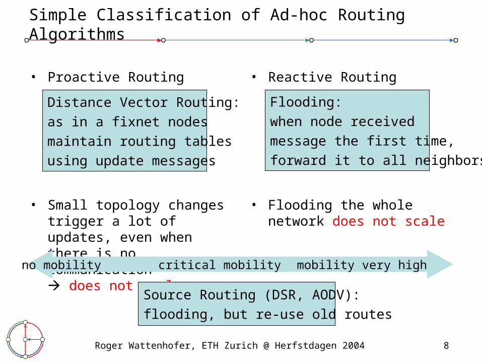
• Proactive Routing
• Small topology changes trigger a lot of updates, even when there is no communication does not scale
Flooding:
when node received
message the first time,
forward it to all neighbors
Distance Vector Routing:
as in a fixnet nodes
maintain routing tables
using update messages
• Reactive Routing
• Flooding the whole network does not scale
no mobility mobility very highcritical mobility
Source Routing (DSR, AODV):
flooding, but re-use old routes

Roger Wattenhofer, ETH Zurich @ Herfstdagen 2004 9
Discussion
• Lecture “Mobile Computing”: 10 Tricks 210 routing algorithms• In reality there are almost that many!
• Q: How good are these routing algorithms?!? Any hard results?• A: Almost none! Method-of-choice is simulation…• Perkins: “if you simulate three times, you get three different results”
• Flooding is key component of (many) proposed algorithms• At least flooding should be efficient

Roger Wattenhofer, ETH Zurich @ Herfstdagen 2004 10
Overview
• Introduction
• Clustering– Flooding vs. Dominating Sets
– Algorithm Overview
– Phase A
– Phase B
– Lower Bounds
• Topology Control• Geo-Routing• Conclusions
Roger Wattenhofer, ETH Zurich @ Herfstdagen 2004 11
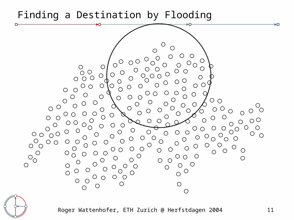
Finding a Destination by Flooding

Roger Wattenhofer, ETH Zurich @ Herfstdagen 2004 12
Finding a Destination Efficiently
Roger Wattenhofer, ETH Zurich @ Herfstdagen 2004 13
(Connected) Dominating Set
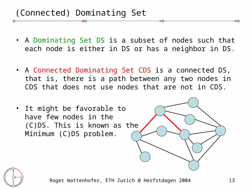
• A Dominating Set DS is a subset of nodes such that each node is either in DS or has a neighbor in DS.
• A Connected Dominating Set CDS is a connected DS, that is, there is a path between any two nodes in CDS that does not use nodes that are not in CDS.
• It might be favorable tohave few nodes in the (C)DS. This is known as theMinimum (C)DS problem.
Roger Wattenhofer, ETH Zurich @ Herfstdagen 2004 14
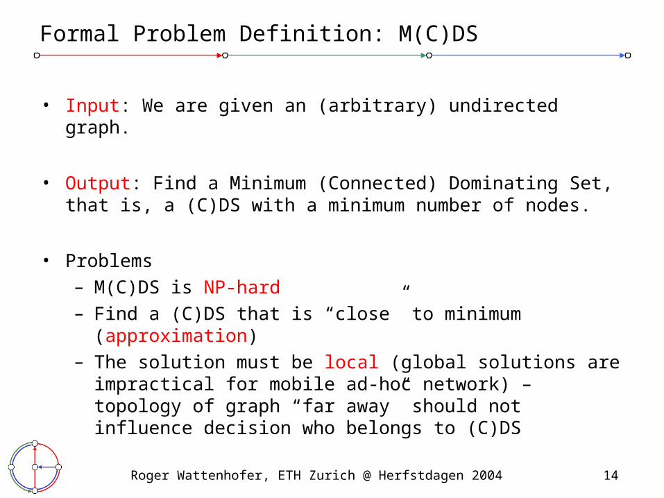
Formal Problem Definition: M(C)DS
• Input: We are given an (arbitrary) undirected graph.
• Output: Find a Minimum (Connected) Dominating Set,that is, a (C)DS with a minimum number of nodes.
• Problems– M(C)DS is NP-hard– Find a (C)DS that is “close” to minimum (approximation)– The solution must be local (global solutions are impractical for
mobile ad-hoc network) – topology of graph “far away” should not influence decision who belongs to (C)DS
Roger Wattenhofer, ETH Zurich @ Herfstdagen 2004 15
Overview
• Introduction
• Clustering– Flooding vs. Dominating Sets
– Algorithm Overview
– Phase A
– Phase B
– Lower Bounds
• Topology Control• Geo-Routing• Conclusions

Roger Wattenhofer, ETH Zurich @ Herfstdagen 2004 16
Algorithm Overview
0.20.5
0.2
0.80
0.2
0.3
0.1
0.3
0
Input:
Local Graph
Fractional
Dominating Set
Dominating
Set
Connected
Dominating Set
0.5
Phase C:
Connect DS
by “tree” of
“bridges”
Phase B:
Probabilistic
algorithm
Phase A:
Distributed
linear programrel. high degree
gives high value

Roger Wattenhofer, ETH Zurich @ Herfstdagen 2004 17
Overview
• Introduction
• Clustering– Flooding vs. Dominating Sets
– Algorithm Overview
– Phase A
– Phase B
– Lower Bounds
• Topology Control• Geo-Routing• Conclusions

Roger Wattenhofer, ETH Zurich @ Herfstdagen 2004 18
Phase A is a Distributed Linear Program
• Nodes 1, …, n: Each node u has variable xu with xu ¸ 0
• Sum of x-values in each neighborhood at least 1 (local)• Minimize sum of all x-values (global)
0.5+0.3+0.3+0.2+0.2+0 = 1.5 ¸ 1
• Linear Programs can be solved optimally in polynomial time• But not in a distributed fashion! That’s what we do here…
0.20.5
0.2
0.80
0.2
0.3
0.1
0.3
0
0.5
Linear Program
Adjacency matrix
with 1’s in diagonal
Roger Wattenhofer, ETH Zurich @ Herfstdagen 2004 19
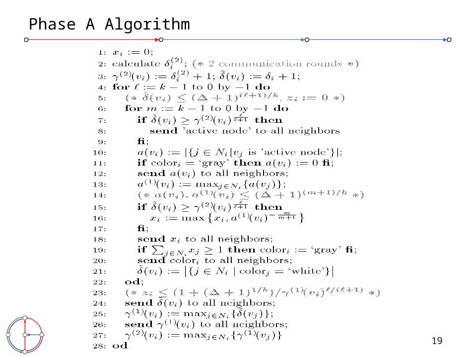
Phase A Algorithm
Roger Wattenhofer, ETH Zurich @ Herfstdagen 2004 20
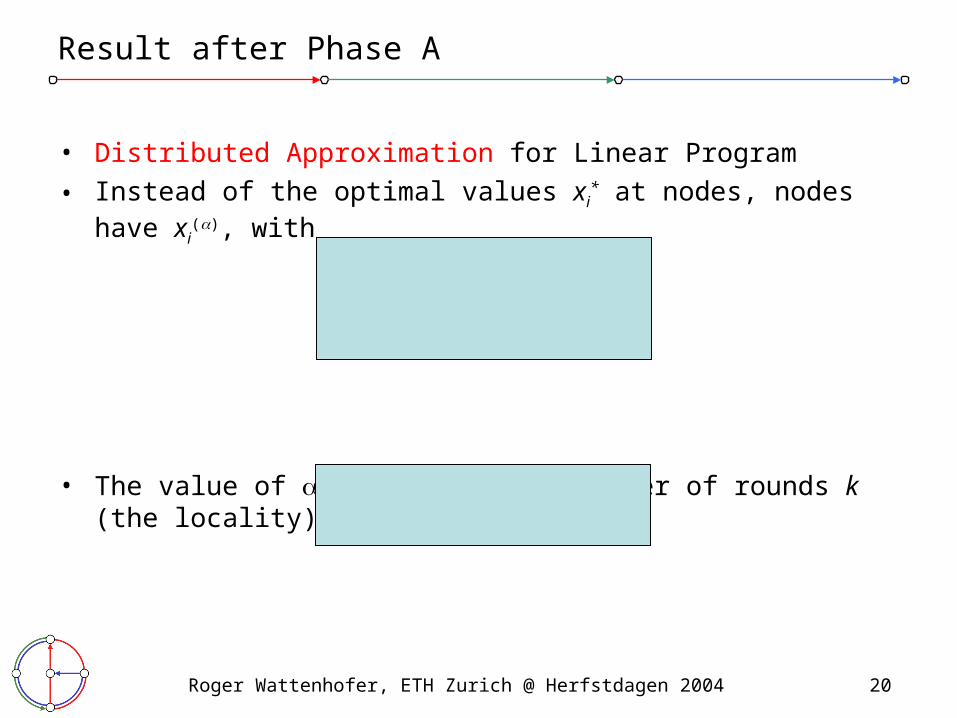
Result after Phase A
• Distributed Approximation for Linear Program
• Instead of the optimal values xi* at nodes, nodes have xi
(), with
• The value of depends on the number of rounds k (the locality)

Roger Wattenhofer, ETH Zurich @ Herfstdagen 2004 21
Overview
• Introduction
• Clustering– Flooding vs. Dominating Sets
– Algorithm Overview
– Phase A
– Phase B
– Lower Bounds
• Topology Control• Geo-Routing• Conclusions

Roger Wattenhofer, ETH Zurich @ Herfstdagen 2004 22
Dominating Set as Integer Program
• What we have after phase A
• What we want after phase B

Roger Wattenhofer, ETH Zurich @ Herfstdagen 2004 23
Phase B Algorithm
Each node applies the following algorithm:
1. Calculate (= maximum degree of neighbors in distance 2)
2. Become a dominator (i.e. go to the dominating set) with probability
3. Send status (dominator or not) to all neighbors
4. If no neighbor is a dominator, become a dominator yourself
From phase A Highest degree in distance 2

Roger Wattenhofer, ETH Zurich @ Herfstdagen 2004 24
Result after Phase B
• Randomized rounding technique
• Expected number of nodes joining the dominating set in step 2 is bounded by log(+1) ¢ |DSOPT|.
• Expected number of nodes joining the dominating set in step 4 is bounded by |DSOPT|.
Theorem: E[|DS|] · O( ln ¢ |DSOPT|)

Roger Wattenhofer, ETH Zurich @ Herfstdagen 2004 25
Related Work on (Connected) Dominating Sets
• Global algorithms – Johnson (1974), Lovasz (1975), Slavik (1996): Greedy is optimal– Guha, Kuller (1996): An optimal algorithm for CDS– Feige (1998): ln lower bound unless NP 2 nO(log log n)
• Local (distributed) algorithms– “Handbook of Wireless Networks and Mobile Computing”: All
algorithms presented have no guarantees– Gao, Guibas, Hershberger, Zhang, Zhu (2001): “Discrete Mobile
Centers” O(loglog n) time, but nodes know coordinates– MIS-based algorithms (e.g. Alzoubi, Wan, Frieder, 2002) that
only work on unit disk graphs.– Kuhn, Wattenhofer (2003): Tradeoff time vs. approximation

Roger Wattenhofer, ETH Zurich @ Herfstdagen 2004 26
Recent Improvements
• Improved algorithms (Kuhn, Wattenhofer, 2004):– O(log2 / 4) time for a (1+)-approximation of phase A with
logarithmic sized messages.– If messages can be of unbounded size there is a constant
approximation of phase A in O(log n) time, using the graph decomposition by Linial and Saks.
– An improved and generalized distributed randomized rounding technique for phase B.
– Works for quite general linear programs.
• Is it any good…?
Roger Wattenhofer, ETH Zurich @ Herfstdagen 2004 27
Overview
• Introduction
• Clustering– Flooding vs. Dominating Sets
– Algorithm Overview
– Phase A
– Phase B
– Lower Bounds
• Topology Control• Geo-Routing• Conclusions

Roger Wattenhofer, ETH Zurich @ Herfstdagen 2004 28
Lower Bound for Dominating Sets: Intuition…
m
n-1
complete
n
m m
…
n n n
• Two graphs (m << n). Optimal dominating sets are marked red.
|DSOPT| = 2.|DSOPT| = m+1.

Roger Wattenhofer, ETH Zurich @ Herfstdagen 2004 29
Lower Bound for Dominating Sets: Intuition…
• In local algorithms, nodes must decide only using local knowledge.• In the example green nodes see exactly the same neighborhood.
• So these green nodes must decide the same way!
m
n-1
n
m
…

Roger Wattenhofer, ETH Zurich @ Herfstdagen 2004 30
Lower Bound for Dominating Sets: Intuition…
m
n-1
complete
n
m m
…
n n n
• But however they decide, one way will be devastating (with n = m2)!
|DSOPT| = 2.
|DSOPT without green| ¸ m.|DSOPT| = m+1.
|DSOPT with green| > n
Roger Wattenhofer, ETH Zurich @ Herfstdagen 2004 31
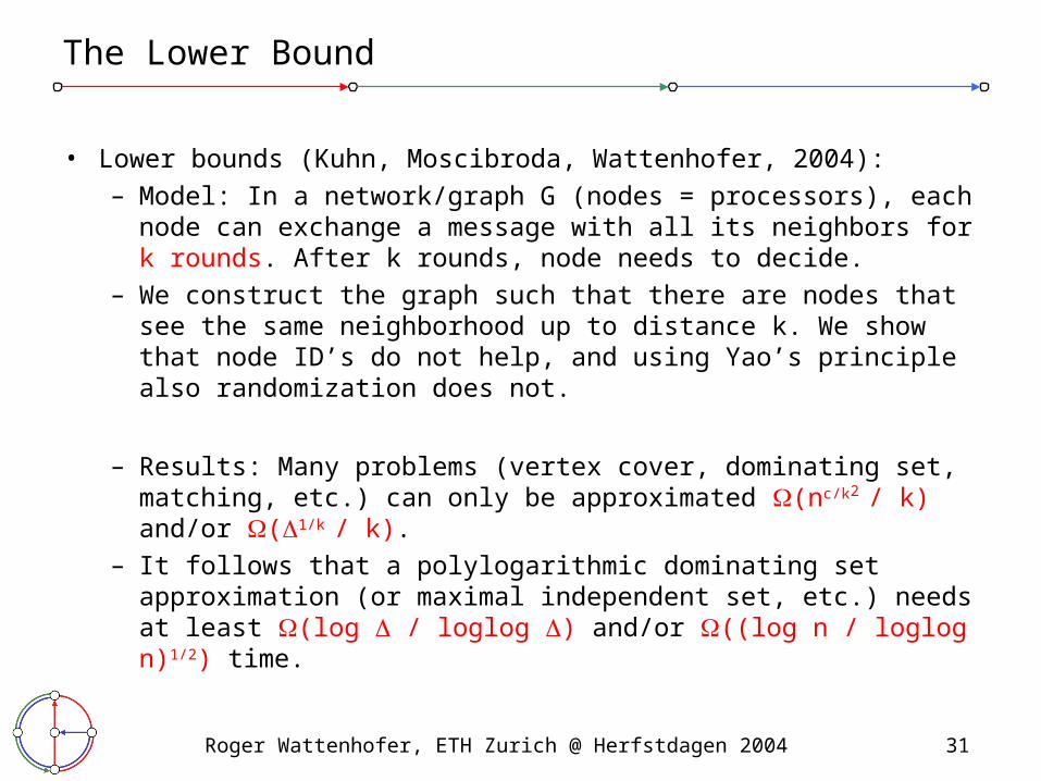
The Lower Bound
• Lower bounds (Kuhn, Moscibroda, Wattenhofer, 2004):– Model: In a network/graph G (nodes = processors), each node
can exchange a message with all its neighbors for k rounds. After k rounds, node needs to decide.
– We construct the graph such that there are nodes that see the same neighborhood up to distance k. We show that node ID’s do not help, and using Yao’s principle also randomization does not.
– Results: Many problems (vertex cover, dominating set, matching, etc.) can only be approximated (nc/k2 / k) and/or (1/k / k).
– It follows that a polylogarithmic dominating set approximation (or maximal independent set, etc.) needs at least (log / loglog ) and/or ((log n / loglog n)1/2) time.

Roger Wattenhofer, ETH Zurich @ Herfstdagen 2004 32
Graph Used in Dominating Set Lower Bound
• The example is for k = 3.• All edges are in fact special bipartite graphs
with large enough girth.

Roger Wattenhofer, ETH Zurich @ Herfstdagen 2004 33
Clustering for Unstructured Radio Networks
• “Big Bang” (deployment) of a sensor and/or ad-hoc network:– Nodes wake up asynchronously (very late, maybe)
– Neighbors unknown
– Hidden terminal problem
– No global clock
– No established MAC protocol
– No reliable collision detection
– Limited knowledge of the number of nodes or degree of network.
• We have randomized algorithms that compute DS (or MIS) in polylog(n) time even under these harsh circumstances, where n is an upper bound on the number of nodes in the system.
• [Kuhn, Moscibroda, Wattenhofer, 2004]
Roger Wattenhofer, ETH Zurich @ Herfstdagen 2004 34
Overview
• Introduction• Clustering
• Topology Control– What is it? What is it good for?
– Does Topology Control Reduce Interference?
– Cellular Networks, Sensor Networks, etc.
• Geo-Routing• Conclusions

Roger Wattenhofer, ETH Zurich @ Herfstdagen 2004 35
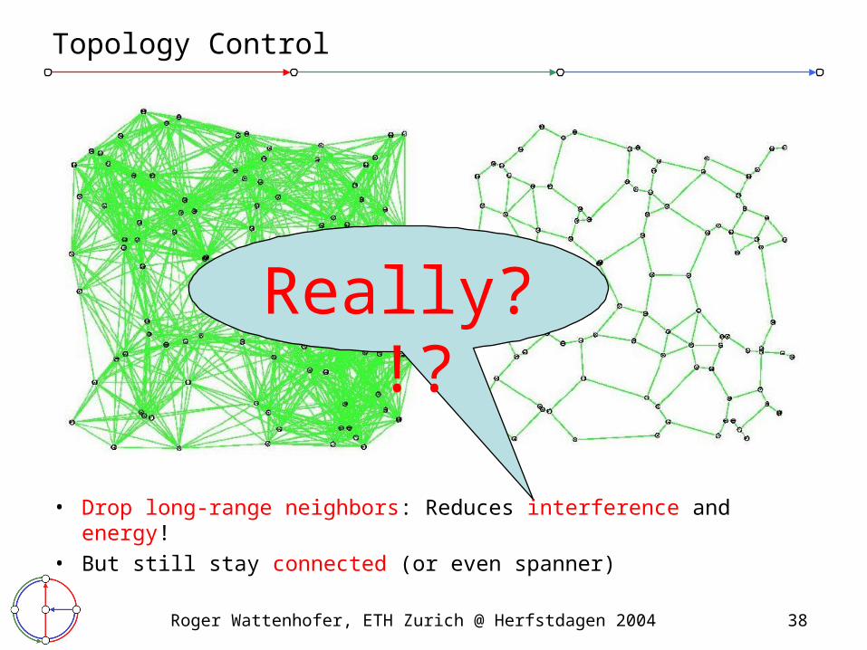
Topology Control
• Drop long-range neighbors: Reduces interference and energy!• But still stay connected (or even spanner)
Roger Wattenhofer, ETH Zurich @ Herfstdagen 2004 36
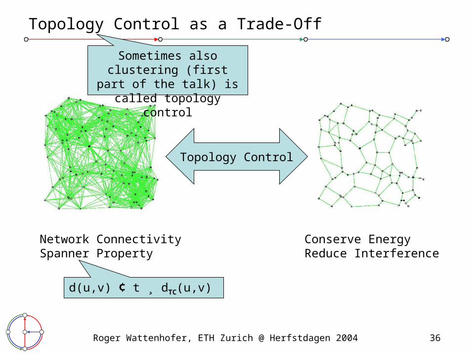
Topology Control as a Trade-Off
Network ConnectivitySpanner Property
Topology Control
Conserve EnergyReduce Interference
Sometimes also clustering (first part of the talk) is called topology control
d(u,v) ¢ t ¸ dTC(u,v)

Roger Wattenhofer, ETH Zurich @ Herfstdagen 2004 37
Classic Solution: Gabriel Graph
• Let disk(u,v) be a disk with diameter (u,v)that is determined by the two points u,v.
• The Gabriel Graph GG(V) is defined as an undirected graph (with E being a set of undirected edges). There is an edge between two nodes u,v iff the disk(u,v) including boundary contains no other points.
• Gabriel Graph is planar• Gabriel Graph is energy optimal
[energy of link is at least distance squared]
disk(u,v)
v
u
Roger Wattenhofer, ETH Zurich @ Herfstdagen 2004 38
Topology Control
• Drop long-range neighbors: Reduces interference and energy!• But still stay connected (or even spanner)
Really?!?

Roger Wattenhofer, ETH Zurich @ Herfstdagen 2004 39
Related Work
• Mid-Eighties: randomly distributed nodes[Takagi & Kleinrock 1984, Hou & Li 1986]
• Second Wave: constructions from computational geometry, Delaunay Triangulation [Hu 1993], Minimum Spanning Tree [Ramanathan & Rosales-Hain INFOCOM 2000], Gabriel Graph [Rodoplu & Meng J.Sel.Ar.Com 1999]
• Cone-Based Topology Control [Wattenhofer et al. INFOCOM 2000]; explicitly prove several properties (energy spanner, sparse graph), locality. Collecting more and more properties [Li et al. PODC 2001, Jia et al. SPAA 2003, Li et al. INFOCOM 2004] (e.g. local, planar, distance and energy spanner, constant node degree)
• Explicit interference [Meyer auf der Heide et al. SPAA 2002]. Interference between edges, time-step routing model, congestion; trade-offs; however, interference model based on network traffic
Roger Wattenhofer, ETH Zurich @ Herfstdagen 2004 40
Overview
• Introduction• Clustering
• Topology Control– What is it? What is it good for?
– Does Topology Control Reduce Interference?
– Cellular Networks, Sensor Networks, etc.
• Geo-Routing• Conclusions
Roger Wattenhofer, ETH Zurich @ Herfstdagen 2004 41
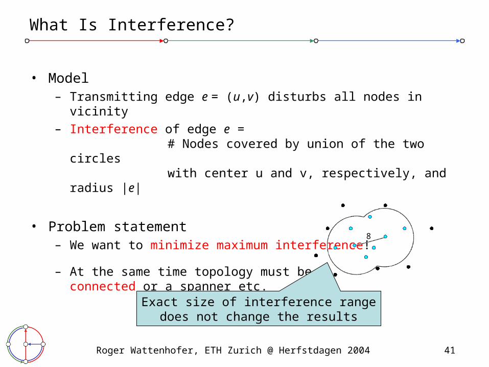
What Is Interference?
• Model– Transmitting edge e = (u,v) disturbs all nodes in vicinity
– Interference of edge e = # Nodes covered by union of the two circles with center u and v, respectively, and radius |e|
• Problem statement– We want to minimize maximum interference!
– At the same time topology must beconnected or a spanner etc. 8
Exact size of interference rangedoes not change the results

Roger Wattenhofer, ETH Zurich @ Herfstdagen 2004 42
Low Node Degree Topology Control?
Low node degree does not necessarily imply low interference:
Very low node degreebut huge interference

Roger Wattenhofer, ETH Zurich @ Herfstdagen 2004 43
Let’s Study the Following Topology!
…from a worst-case perspective

Roger Wattenhofer, ETH Zurich @ Herfstdagen 2004 44
Topology Control Algorithms Produce…
• All known topology control algorithms (with symmetric edges) include the nearest neighbor forest as a subgraph and produce something like this:
• The interference of this graph is (n)!

Roger Wattenhofer, ETH Zurich @ Herfstdagen 2004 45
But Interference…
• Interference does not need to be high…
• This topology has interference O(1)!!

Roger Wattenhofer, ETH Zurich @ Herfstdagen 2004 46
Algorithms and Lower Bounds
• [Burkhart, von Rickenbach, Wattenhofer, Zollinger, 2004]• Interference-optimal connectivity-preserving topology• Local interference-optimal spanner topology• Algorithms also work if interference radius >> transmission radius• No local algorithm can find a good topology• Optimal topology is not planar
UDG, I = 50 RNG, I = 25 LLISE10, I = 12

Roger Wattenhofer, ETH Zurich @ Herfstdagen 2004 47
Overview
• Introduction• Clustering
• Topology Control– What is it? What is it good for?
– Does Topology Control Reduce Interference?
– Cellular Networks, Sensor Networks, etc.
• Geo-Routing• Conclusions

Roger Wattenhofer, ETH Zurich @ Herfstdagen 2004 48
New Results…
• Interference-driven topology control is exciting new paradigm…
• We have a few other upcoming results:
• For cellular networks: minimize number of base stations a mobile station overhears by reducing the transmission power of the base stations “minimum membership set cover” problem
• For sensor networks: data gathering without listening to lots of unwanted traffic…
Roger Wattenhofer, ETH Zurich @ Herfstdagen 2004 49
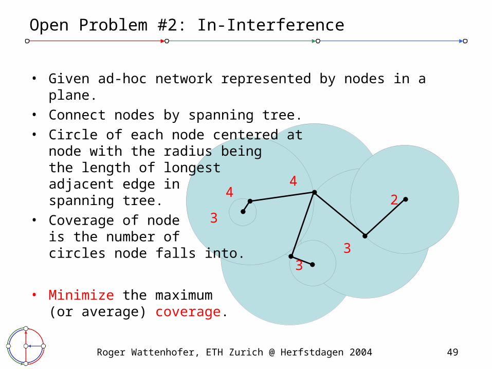
Open Problem #2: In-Interference
• Given ad-hoc network represented by nodes in a plane.• Connect nodes by spanning tree.• Circle of each node centered at
node with the radius being the length of longest adjacent edge in spanning tree.
• Coverage of node is the number of circles node falls into.
• Minimize the maximum (or average) coverage.
3
4
3
24
3
Roger Wattenhofer, ETH Zurich @ Herfstdagen 2004 50
Overview
• Introduction• Clustering• Topology Control
• Geo-Routing– What is geometric routing?
– Correct geometric routing
– Worst-case efficient geometric routing
– Average-case efficient geometric routing
• Conclusions

Roger Wattenhofer, ETH Zurich @ Herfstdagen 2004 51
Geometric Routing
t
s
s
???

Roger Wattenhofer, ETH Zurich @ Herfstdagen 2004 52
Greedy Routing
• Each node forwards message to “best” neighbor
t
s

Roger Wattenhofer, ETH Zurich @ Herfstdagen 2004 53
Greedy Routing
• Each node forwards message to “best” neighbor
• But greedy routing may fail: message may get stuck in a “dead end”• Needed: Correct geometric routing algorithm
t
?s

Roger Wattenhofer, ETH Zurich @ Herfstdagen 2004 54
What is Geometric Routing?
• A.k.a. location-based, position-based, geographic, etc.• Chapter 18 (“Routing […] in Geometric and Wireless Networks”) in
“Handbook of Wireless Networking and Mobile Computing”
• Each node knows its own position and position of neighbors• Source knows the position of the destination• No routing tables stored in nodes!
• Geometric routing makes sense– Own position: GPS/Galileo, local positioning algorithm– Destination: overlay P2P net, geocasting, source routing++– Learn about ad-hoc routing in general
Roger Wattenhofer, ETH Zurich @ Herfstdagen 2004 55
Overview
• Introduction• Clustering• Topology Control
• Geo-Routing– What is geometric routing?
– Correct geometric routing
– Worst-case efficient geometric routing
– Average-case efficient geometric routing
• Conclusions
Roger Wattenhofer, ETH Zurich @ Herfstdagen 2004 56
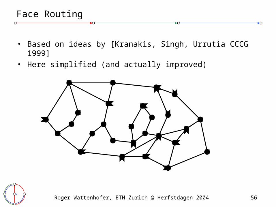
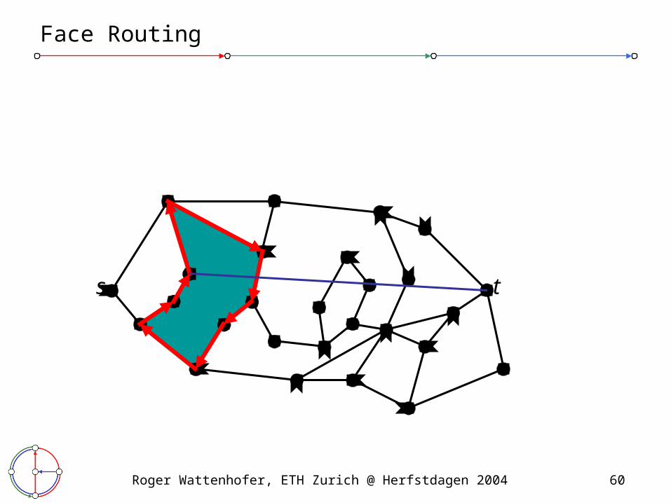
Face Routing
• Based on ideas by [Kranakis, Singh, Urrutia CCCG 1999]• Here simplified (and actually improved)
Roger Wattenhofer, ETH Zurich @ Herfstdagen 2004 57
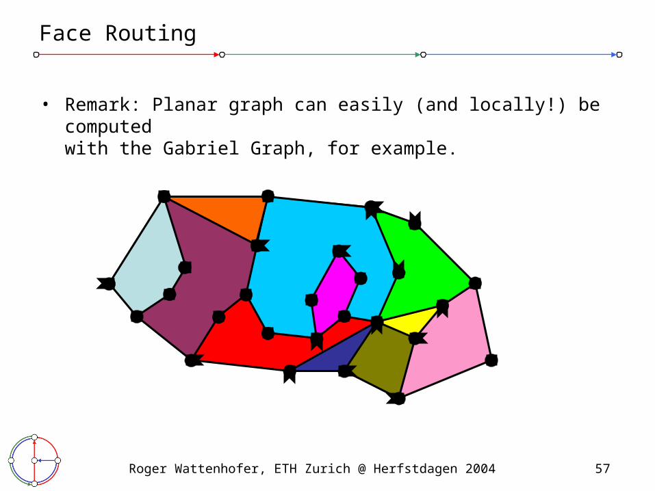
Face Routing
• Remark: Planar graph can easily (and locally!) be computed with the Gabriel Graph, for example.

Roger Wattenhofer, ETH Zurich @ Herfstdagen 2004 58
Face Routing
s t

Roger Wattenhofer, ETH Zurich @ Herfstdagen 2004 59
Face Routing
s t
Roger Wattenhofer, ETH Zurich @ Herfstdagen 2004 60
Face Routing
s t

Roger Wattenhofer, ETH Zurich @ Herfstdagen 2004 61
Face Routing
s t

Roger Wattenhofer, ETH Zurich @ Herfstdagen 2004 62
Face Routing
s t

Roger Wattenhofer, ETH Zurich @ Herfstdagen 2004 63
Face Routing
s t
Roger Wattenhofer, ETH Zurich @ Herfstdagen 2004 64
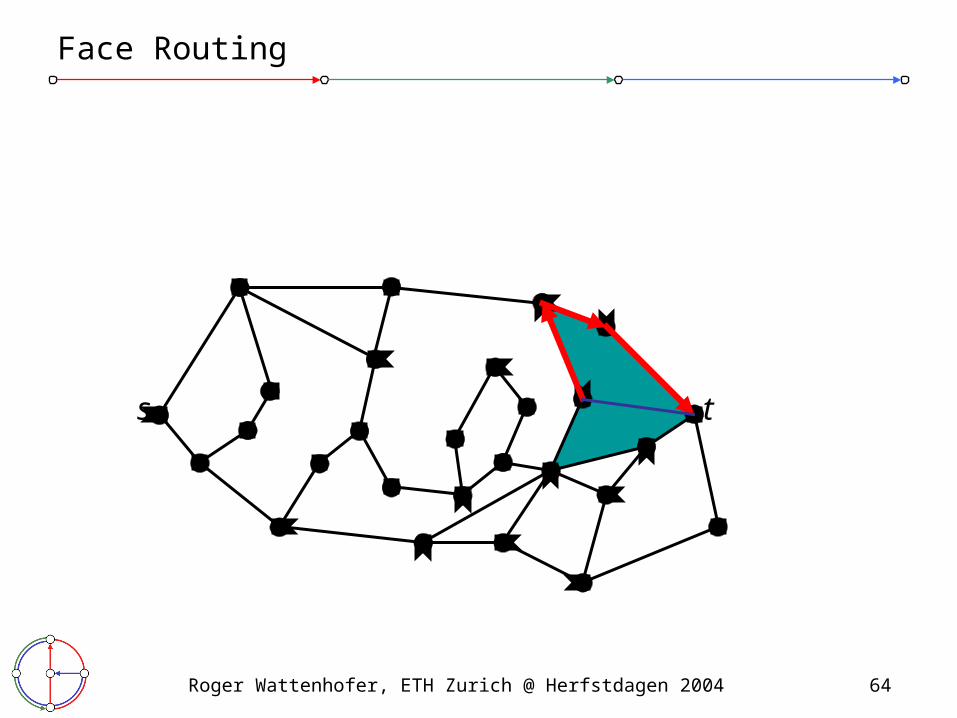
Face Routing
s t

Roger Wattenhofer, ETH Zurich @ Herfstdagen 2004 65
• All necessary information is stored in the message– Source and destination positions
– Point of transition to next face
• Completely local:– Knowledge about direct neighbors‘ positions sufficient
– Faces are implicit
• Planarity of graph is computed locally (not an assumption)
Face Routing Properties
“Right Hand Rule”

Roger Wattenhofer, ETH Zurich @ Herfstdagen 2004 66
Face Routing Works on Any Graph
s
t

Roger Wattenhofer, ETH Zurich @ Herfstdagen 2004 67
Overview
• Introduction• Clustering• Topology Control
• Geo-Routing– What is geometric routing?
– Correct geometric routing
– Worst-case efficient geometric routing
– Average-case efficient geometric routing
• Conclusions

Roger Wattenhofer, ETH Zurich @ Herfstdagen 2004 68
Face Routing
• Theorem: Face Routing reaches destination in O(n) steps• But: Can be very bad compared to the optimal route
Roger Wattenhofer, ETH Zurich @ Herfstdagen 2004 69
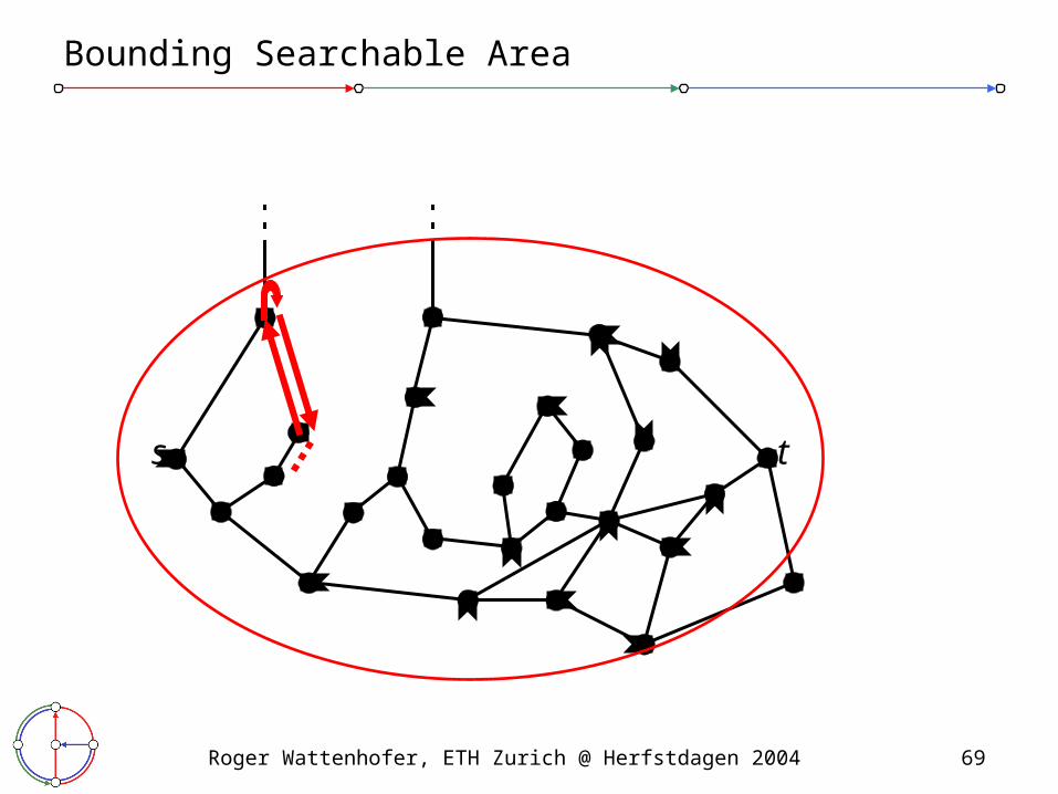
Bounding Searchable Area
ts

Roger Wattenhofer, ETH Zurich @ Herfstdagen 2004 70
Adaptively Bound Searchable Area
• What is the correct size of the bounding area?– Start with a small searchable area
– Grow area each time you cannot reach the destination
– In other words, adapt area size whenever it is too small
Theorem: Algorithm finds destination after O(c2) steps, where c is the cost of the optimal path from source to destination.
• Proof: Not in this presentation.
Roger Wattenhofer, ETH Zurich @ Herfstdagen 2004 71
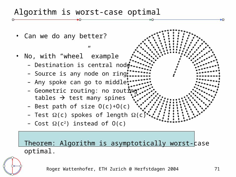
Algorithm is worst-case optimal
• Can we do any better?
• No, with “wheel” example– Destination is central node
– Source is any node on ring
– Any spoke can go to middle
– Geometric routing: no routingtables test many spines
– Best path of size O(c)+O(c)
– Test (c) spokes of length (c)
– Cost (c2) instead of O(c)
Theorem: Algorithm is asymptotically worst-case optimal.

Roger Wattenhofer, ETH Zurich @ Herfstdagen 2004 72
Overview
• Introduction• Clustering• Topology Control
• Geo-Routing– What is geometric routing?
– Correct geometric routing
– Worst-case efficient geometric routing
– Average-case efficient geometric routing
• Conclusions
Roger Wattenhofer, ETH Zurich @ Herfstdagen 2004 73
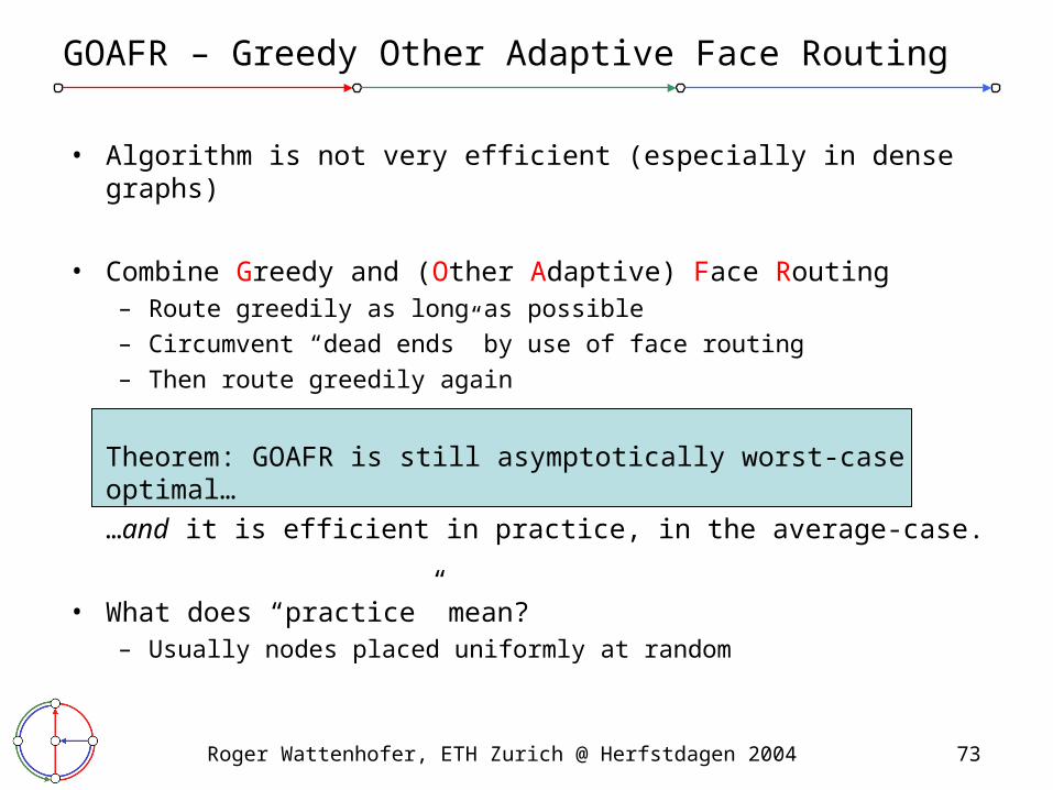
GOAFR – Greedy Other Adaptive Face Routing
• Algorithm is not very efficient (especially in dense graphs)
• Combine Greedy and (Other Adaptive) Face Routing– Route greedily as long as possible
– Circumvent “dead ends” by use of face routing
– Then route greedily again
Theorem: GOAFR is still asymptotically worst-case optimal…
…and it is efficient in practice, in the average-case.
• What does “practice” mean?– Usually nodes placed uniformly at random

Roger Wattenhofer, ETH Zurich @ Herfstdagen 2004 74
Average Case
• Not interesting when graph not dense enough• Not interesting when graph is too dense• Critical density range (“percolation”)
– Shortest path is significantly longer than Euclidean distance
too sparse too densecritical density

Roger Wattenhofer, ETH Zurich @ Herfstdagen 2004 75
• Shortest path is significantly longer than Euclidean distance
• Critical density range mandatory for the simulation of any routing algorithm (not only geometric)
Critical Density: Shortest Path vs. Euclidean Distance

Roger Wattenhofer, ETH Zurich @ Herfstdagen 2004 76
Simulation on Randomly Generated Graphs
GFG/GPSR
GOAFR+
Greedy success
Connectivity
bett
erw
orse
1
2
3
4
5
6
7
8
9
0 2 4 6 8 10 12
Network Density [nodes per unit disk]
Pe
rfo
rma
nce
0
0.1
0.2
0.3
0.4
0.5
0.6
0.7
0.8
0.9
1
Fre
qu
en
cy
critical

Roger Wattenhofer, ETH Zurich @ Herfstdagen 2004 77
Discussion
• Previously known– Non-competitive algorithms (Face Routing, GFG/GPSR, …)
• Three papers [DIALM 2002, MOBIHOC 2003, PODC 2003]:– The first worst-case optimal algorithm– The first worst-case optimal and average-case efficient algorithm– Percolation theory to evaluate routing algorithms– Various results for different cost metrics (“super-linear” not competitive)– Various related results (“bounded degree graphs”)
• Algorithm is simple: Can be implemented in network processor• Quite a few implementations available• Algorithm can be married with other approaches• Geometric routing as a more stable form of source routing• First tight result in ad-hoc routing (to our knowledge)
Roger Wattenhofer, ETH Zurich @ Herfstdagen 2004 78
Overview
• Introduction• Clustering• Topology Control• Geo-Routing
• Conclusions– Clustering vs. Topology Control
– More realism, more realism, more realism, …
– … Practice!

Roger Wattenhofer, ETH Zurich @ Herfstdagen 2004 79
Clustering vs. Topology Control
• Clustering• (Connected) Dominating Set• (Connected) Domatic Partition
Both approaches sparsen the graph in order to reduce energy…
• … by turning off fraction of the nodes, and thus interference.
Two sides of the same medal?
• Topology Control• Interference-Driven T.C.
• … by turning off long-range links, and thus interference.

Roger Wattenhofer, ETH Zurich @ Herfstdagen 2004 80
Overview
• Introduction• Clustering• Topology Control• Geo-Routing
• Conclusions– Clustering vs. Topology Control
– More realism, more realism, more realism, …
– … Practice!

81
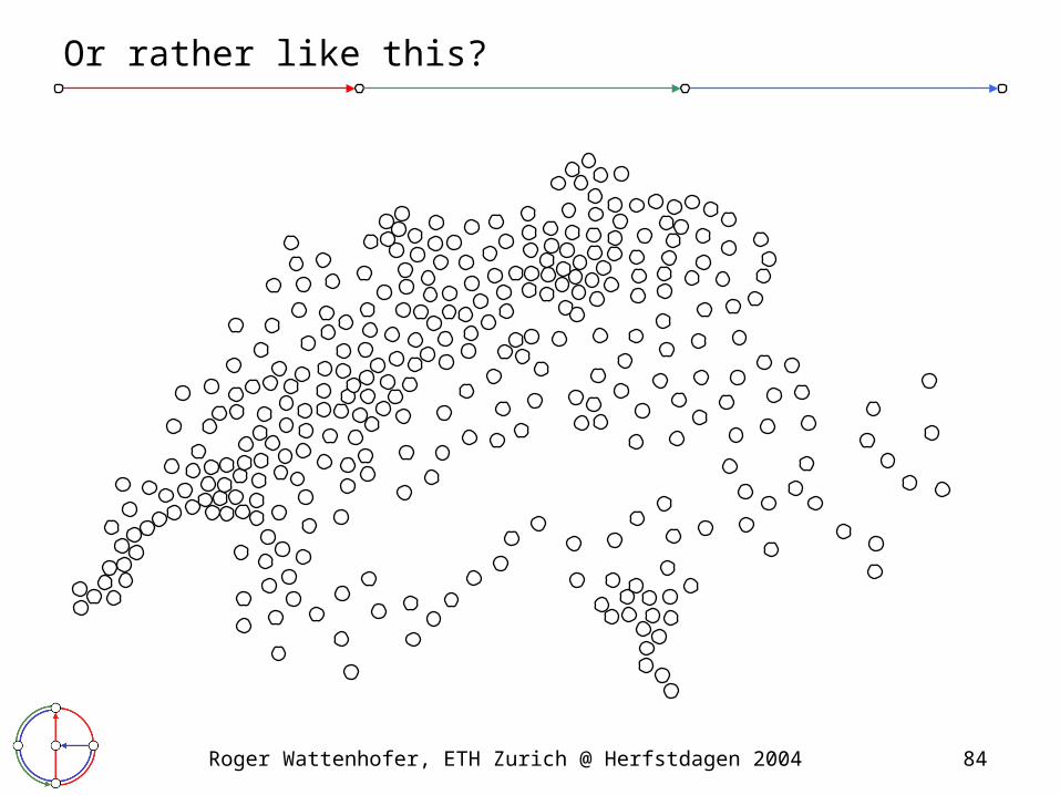
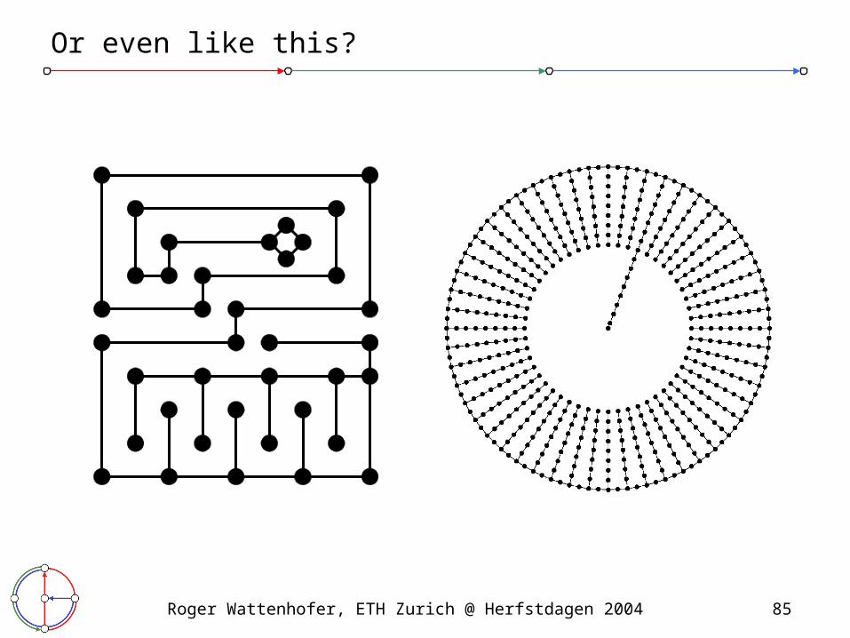
?What does a
typical ad-hoc network
look like?

Roger Wattenhofer, ETH Zurich @ Herfstdagen 2004 82
Like this?

Roger Wattenhofer, ETH Zurich @ Herfstdagen 2004 83
Like this?
Roger Wattenhofer, ETH Zurich @ Herfstdagen 2004 84
Or rather like this?
Roger Wattenhofer, ETH Zurich @ Herfstdagen 2004 85
Or even like this?

Roger Wattenhofer, ETH Zurich @ Herfstdagen 2004 86
What about typical mobility?
• Brownian Motion?
• Random Way-Point?
• Statistical Data Model?
• Maximum Speed Model?
• …?

Roger Wattenhofer, ETH Zurich @ Herfstdagen 2004 87
Overview
• Introduction• Clustering• Topology Control• Geo-Routing
• Conclusions– Clustering vs. Topology Control
– More realism, more realism, more realism, …
– … Practice!
Roger Wattenhofer, ETH Zurich @ Herfstdagen 2004 88
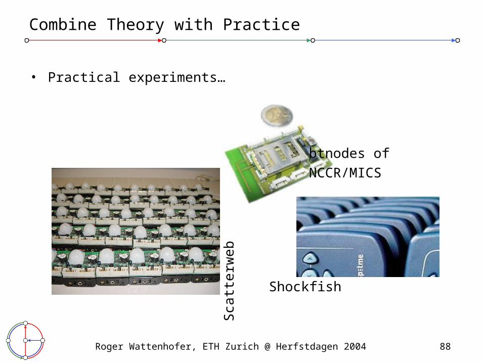
Combine Theory with Practice
• Practical experiments…
Shockfish
btnodes of
NCCR/MICS
Sca
tterw
eb

Roger Wattenhofer, ETH Zurich @ Herfstdagen 2004 89
Some credit…
Problem (Algorithm) Reference
Dominating Set Kuhn, W. @ PODC 2003Kuhn, Moscibroda, W. @ PODC 2004
Topology Control and Interference (LISE, XTC, MMSC, Sensor Networks)
Burkhart et al. @ MobiHoc 2004W., Zollinger @ WMAN 2004von Rickenbach et al. @ submittedZollinger et al. @ submitted
Geo-Routing (GOAFR) Kuhn, W., Zollinger @ MobiHoc 2003Kuhn, W., Zhang, Zollinger @ PODC 2003
Positioning (GHoST) Bischoff, W. @ PerCom 2004Kuhn, Moscibroda, W. @ DIALM 2004Moscibroda et al. @ DIALM 2004.
Data gathering Cristescu et al. @ submittedvon Rickenbach, W. @ DIALM 2004
Models: Quasi-UDG Kuhn, W., Zollinger @ DIALM 2003
“Deployment” problem Moscibroda, W. @ ESA & MobiCom & MASS 2004
90
Thank you!
DistributedComputing
GroupRoger Wattenhofer