algorithms and data structures for mathematicians ...kostolanyi/ads/lec01.pdf · algorithms...
TRANSCRIPT

Algorithms and Data Structuresfor Mathematicians
Lecture 1: An Introduction
Peter Kostolányikostolanyi at fmph and so on
Room M-258
28 September 2017
Some Not Really Formal Definitions
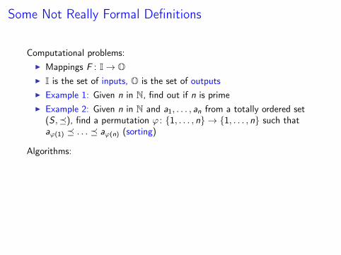
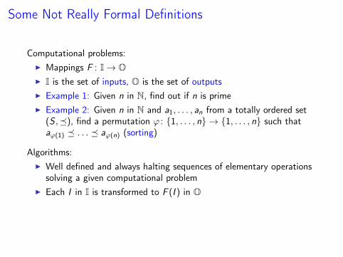
Computational problems:
I Mappings F : I→ OI I is the set of inputs, O is the set of outputsI Example 1: Given n in N, find out if n is primeI Example 2: Given n in N and a1, . . . , an from a totally ordered set
(S ,), find a permutation ϕ : 1, . . . , n → 1, . . . , n such thataϕ(1) . . . aϕ(n) (sorting)
Algorithms:I Well defined and always halting sequences of elementary operations
solving a given computational problemI Each I in I is transformed to F (I ) in OI Might or might not be implemented on a computerI We shall be particularly interested in efficient algorithms

Some Not Really Formal Definitions
Computational problems:I Mappings F : I→ O
I I is the set of inputs, O is the set of outputsI Example 1: Given n in N, find out if n is primeI Example 2: Given n in N and a1, . . . , an from a totally ordered set
(S ,), find a permutation ϕ : 1, . . . , n → 1, . . . , n such thataϕ(1) . . . aϕ(n) (sorting)
Algorithms:I Well defined and always halting sequences of elementary operations
solving a given computational problemI Each I in I is transformed to F (I ) in OI Might or might not be implemented on a computerI We shall be particularly interested in efficient algorithms

Some Not Really Formal Definitions
Computational problems:I Mappings F : I→ OI I is the set of inputs, O is the set of outputs
I Example 1: Given n in N, find out if n is primeI Example 2: Given n in N and a1, . . . , an from a totally ordered set
(S ,), find a permutation ϕ : 1, . . . , n → 1, . . . , n such thataϕ(1) . . . aϕ(n) (sorting)
Algorithms:I Well defined and always halting sequences of elementary operations
solving a given computational problemI Each I in I is transformed to F (I ) in OI Might or might not be implemented on a computerI We shall be particularly interested in efficient algorithms

Some Not Really Formal Definitions
Computational problems:I Mappings F : I→ OI I is the set of inputs, O is the set of outputsI Example 1: Given n in N, find out if n is prime
I Example 2: Given n in N and a1, . . . , an from a totally ordered set(S ,), find a permutation ϕ : 1, . . . , n → 1, . . . , n such thataϕ(1) . . . aϕ(n) (sorting)
Algorithms:I Well defined and always halting sequences of elementary operations
solving a given computational problemI Each I in I is transformed to F (I ) in OI Might or might not be implemented on a computerI We shall be particularly interested in efficient algorithms

Some Not Really Formal Definitions
Computational problems:I Mappings F : I→ OI I is the set of inputs, O is the set of outputsI Example 1: Given n in N, find out if n is primeI Example 2: Given n in N and a1, . . . , an from a totally ordered set
(S ,), find a permutation ϕ : 1, . . . , n → 1, . . . , n such thataϕ(1) . . . aϕ(n) (sorting)
Algorithms:I Well defined and always halting sequences of elementary operations
solving a given computational problemI Each I in I is transformed to F (I ) in OI Might or might not be implemented on a computerI We shall be particularly interested in efficient algorithms
Some Not Really Formal Definitions
Computational problems:I Mappings F : I→ OI I is the set of inputs, O is the set of outputsI Example 1: Given n in N, find out if n is primeI Example 2: Given n in N and a1, . . . , an from a totally ordered set
(S ,), find a permutation ϕ : 1, . . . , n → 1, . . . , n such thataϕ(1) . . . aϕ(n) (sorting)
Algorithms:
I Well defined and always halting sequences of elementary operationssolving a given computational problem
I Each I in I is transformed to F (I ) in OI Might or might not be implemented on a computerI We shall be particularly interested in efficient algorithms

Some Not Really Formal Definitions
Computational problems:I Mappings F : I→ OI I is the set of inputs, O is the set of outputsI Example 1: Given n in N, find out if n is primeI Example 2: Given n in N and a1, . . . , an from a totally ordered set
(S ,), find a permutation ϕ : 1, . . . , n → 1, . . . , n such thataϕ(1) . . . aϕ(n) (sorting)
Algorithms:I Well defined and always halting sequences of elementary operations
solving a given computational problem
I Each I in I is transformed to F (I ) in OI Might or might not be implemented on a computerI We shall be particularly interested in efficient algorithms
Some Not Really Formal Definitions
Computational problems:I Mappings F : I→ OI I is the set of inputs, O is the set of outputsI Example 1: Given n in N, find out if n is primeI Example 2: Given n in N and a1, . . . , an from a totally ordered set
(S ,), find a permutation ϕ : 1, . . . , n → 1, . . . , n such thataϕ(1) . . . aϕ(n) (sorting)
Algorithms:I Well defined and always halting sequences of elementary operations
solving a given computational problemI Each I in I is transformed to F (I ) in O
I Might or might not be implemented on a computerI We shall be particularly interested in efficient algorithms

Some Not Really Formal Definitions
Computational problems:I Mappings F : I→ OI I is the set of inputs, O is the set of outputsI Example 1: Given n in N, find out if n is primeI Example 2: Given n in N and a1, . . . , an from a totally ordered set
(S ,), find a permutation ϕ : 1, . . . , n → 1, . . . , n such thataϕ(1) . . . aϕ(n) (sorting)
Algorithms:I Well defined and always halting sequences of elementary operations
solving a given computational problemI Each I in I is transformed to F (I ) in OI Might or might not be implemented on a computer
I We shall be particularly interested in efficient algorithms

Some Not Really Formal Definitions
Computational problems:I Mappings F : I→ OI I is the set of inputs, O is the set of outputsI Example 1: Given n in N, find out if n is primeI Example 2: Given n in N and a1, . . . , an from a totally ordered set
(S ,), find a permutation ϕ : 1, . . . , n → 1, . . . , n such thataϕ(1) . . . aϕ(n) (sorting)
Algorithms:I Well defined and always halting sequences of elementary operations
solving a given computational problemI Each I in I is transformed to F (I ) in OI Might or might not be implemented on a computerI We shall be particularly interested in efficient algorithms

Some Not Really Formal Definitions
Data Structures:
I Representations of data in memory (e.g., arrays, linked lists, . . . )I Aim: to access and/or modify data efficiently
Design and analysis of algorithms (and data structures):I Can make programming efficient, but is not programmingI Uses some elementary mathematics, but is not mathematicsI A truly mathematical approach: computation theory
I 2-MPG-218 Complexity theory (this summer)

Some Not Really Formal Definitions
Data Structures:I Representations of data in memory (e.g., arrays, linked lists, . . . )
I Aim: to access and/or modify data efficiently
Design and analysis of algorithms (and data structures):I Can make programming efficient, but is not programmingI Uses some elementary mathematics, but is not mathematicsI A truly mathematical approach: computation theory
I 2-MPG-218 Complexity theory (this summer)

Some Not Really Formal Definitions
Data Structures:I Representations of data in memory (e.g., arrays, linked lists, . . . )I Aim: to access and/or modify data efficiently
Design and analysis of algorithms (and data structures):
I Can make programming efficient, but is not programmingI Uses some elementary mathematics, but is not mathematicsI A truly mathematical approach: computation theory
I 2-MPG-218 Complexity theory (this summer)

Some Not Really Formal Definitions
Data Structures:I Representations of data in memory (e.g., arrays, linked lists, . . . )I Aim: to access and/or modify data efficiently
Design and analysis of algorithms (and data structures):I Can make programming efficient, but is not programming
I Uses some elementary mathematics, but is not mathematicsI A truly mathematical approach: computation theory
I 2-MPG-218 Complexity theory (this summer)

Some Not Really Formal Definitions
Data Structures:I Representations of data in memory (e.g., arrays, linked lists, . . . )I Aim: to access and/or modify data efficiently
Design and analysis of algorithms (and data structures):I Can make programming efficient, but is not programmingI Uses some elementary mathematics, but is not mathematics
I A truly mathematical approach: computation theoryI 2-MPG-218 Complexity theory (this summer)

Some Not Really Formal Definitions
Data Structures:I Representations of data in memory (e.g., arrays, linked lists, . . . )I Aim: to access and/or modify data efficiently
Design and analysis of algorithms (and data structures):I Can make programming efficient, but is not programmingI Uses some elementary mathematics, but is not mathematicsI A truly mathematical approach: computation theory
I 2-MPG-218 Complexity theory (this summer)

Some Not Really Formal Definitions
Data Structures:I Representations of data in memory (e.g., arrays, linked lists, . . . )I Aim: to access and/or modify data efficiently
Design and analysis of algorithms (and data structures):I Can make programming efficient, but is not programmingI Uses some elementary mathematics, but is not mathematicsI A truly mathematical approach: computation theory
I 2-MPG-218 Complexity theory (this summer)

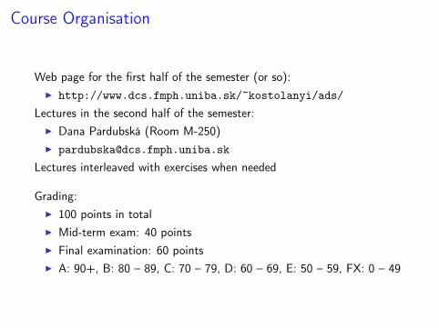
Course Organisation
Web page for the first half of the semester (or so):
I http://www.dcs.fmph.uniba.sk/~kostolanyi/ads/
Lectures in the second half of the semester:I Dana Pardubská (Room M-250)I [email protected]
Lectures interleaved with exercises when needed
Grading:I 100 points in totalI Mid-term exam: 40 pointsI Final examination: 60 pointsI A: 90+, B: 80 – 89, C: 70 – 79, D: 60 – 69, E: 50 – 59, FX: 0 – 49

Course Organisation
Web page for the first half of the semester (or so):I http://www.dcs.fmph.uniba.sk/~kostolanyi/ads/
Lectures in the second half of the semester:
I Dana Pardubská (Room M-250)I [email protected]
Lectures interleaved with exercises when needed
Grading:I 100 points in totalI Mid-term exam: 40 pointsI Final examination: 60 pointsI A: 90+, B: 80 – 89, C: 70 – 79, D: 60 – 69, E: 50 – 59, FX: 0 – 49

Course Organisation
Web page for the first half of the semester (or so):I http://www.dcs.fmph.uniba.sk/~kostolanyi/ads/
Lectures in the second half of the semester:I Dana Pardubská (Room M-250)
Lectures interleaved with exercises when needed
Grading:I 100 points in totalI Mid-term exam: 40 pointsI Final examination: 60 pointsI A: 90+, B: 80 – 89, C: 70 – 79, D: 60 – 69, E: 50 – 59, FX: 0 – 49

Course Organisation
Web page for the first half of the semester (or so):I http://www.dcs.fmph.uniba.sk/~kostolanyi/ads/
Lectures in the second half of the semester:I Dana Pardubská (Room M-250)I [email protected]
Lectures interleaved with exercises when needed
Grading:I 100 points in totalI Mid-term exam: 40 pointsI Final examination: 60 pointsI A: 90+, B: 80 – 89, C: 70 – 79, D: 60 – 69, E: 50 – 59, FX: 0 – 49

Course Organisation
Web page for the first half of the semester (or so):I http://www.dcs.fmph.uniba.sk/~kostolanyi/ads/
Lectures in the second half of the semester:I Dana Pardubská (Room M-250)I [email protected]
Lectures interleaved with exercises when needed
Grading:
I 100 points in totalI Mid-term exam: 40 pointsI Final examination: 60 pointsI A: 90+, B: 80 – 89, C: 70 – 79, D: 60 – 69, E: 50 – 59, FX: 0 – 49

Course Organisation
Web page for the first half of the semester (or so):I http://www.dcs.fmph.uniba.sk/~kostolanyi/ads/
Lectures in the second half of the semester:I Dana Pardubská (Room M-250)I [email protected]
Lectures interleaved with exercises when needed
Grading:I 100 points in total
I Mid-term exam: 40 pointsI Final examination: 60 pointsI A: 90+, B: 80 – 89, C: 70 – 79, D: 60 – 69, E: 50 – 59, FX: 0 – 49

Course Organisation
Web page for the first half of the semester (or so):I http://www.dcs.fmph.uniba.sk/~kostolanyi/ads/
Lectures in the second half of the semester:I Dana Pardubská (Room M-250)I [email protected]
Lectures interleaved with exercises when needed
Grading:I 100 points in totalI Mid-term exam: 40 points
I Final examination: 60 pointsI A: 90+, B: 80 – 89, C: 70 – 79, D: 60 – 69, E: 50 – 59, FX: 0 – 49

Course Organisation
Web page for the first half of the semester (or so):I http://www.dcs.fmph.uniba.sk/~kostolanyi/ads/
Lectures in the second half of the semester:I Dana Pardubská (Room M-250)I [email protected]
Lectures interleaved with exercises when needed
Grading:I 100 points in totalI Mid-term exam: 40 pointsI Final examination: 60 points
I A: 90+, B: 80 – 89, C: 70 – 79, D: 60 – 69, E: 50 – 59, FX: 0 – 49
Course Organisation
Web page for the first half of the semester (or so):I http://www.dcs.fmph.uniba.sk/~kostolanyi/ads/
Lectures in the second half of the semester:I Dana Pardubská (Room M-250)I [email protected]
Lectures interleaved with exercises when needed
Grading:I 100 points in totalI Mid-term exam: 40 pointsI Final examination: 60 pointsI A: 90+, B: 80 – 89, C: 70 – 79, D: 60 – 69, E: 50 – 59, FX: 0 – 49

Suggested Textbooks
Principal Sources:
I Cormen, T. H., Leiserson, C. E., Rivest, R. L., Stein, C.:Introduction to Algorithms, 3rd edition.Cambridge : MIT Press, 2009.
I Aho, A. V., Hopcroft, J. E., Ullman, J. D.:The Design and Analysis of Computer Algorithms.Reading : Addison-Wesley, 1974.
A Book Including Implementations (in Java):I Sedgewick, R., Wayne, K.:
Algorithms, 4th edition.Upper Saddle River : Addison-Wesley, 2011.
A More Gentle Introduction:I Cormen, T. H.:
Algorithms Unlocked.Cambridge : MIT Press, 2013.

Suggested Textbooks
Principal Sources:I Cormen, T. H., Leiserson, C. E., Rivest, R. L., Stein, C.:
Introduction to Algorithms, 3rd edition.Cambridge : MIT Press, 2009.
I Aho, A. V., Hopcroft, J. E., Ullman, J. D.:The Design and Analysis of Computer Algorithms.Reading : Addison-Wesley, 1974.
A Book Including Implementations (in Java):
I Sedgewick, R., Wayne, K.:Algorithms, 4th edition.Upper Saddle River : Addison-Wesley, 2011.
A More Gentle Introduction:I Cormen, T. H.:
Algorithms Unlocked.Cambridge : MIT Press, 2013.

Suggested Textbooks
Principal Sources:I Cormen, T. H., Leiserson, C. E., Rivest, R. L., Stein, C.:
Introduction to Algorithms, 3rd edition.Cambridge : MIT Press, 2009.
I Aho, A. V., Hopcroft, J. E., Ullman, J. D.:The Design and Analysis of Computer Algorithms.Reading : Addison-Wesley, 1974.
A Book Including Implementations (in Java):I Sedgewick, R., Wayne, K.:
Algorithms, 4th edition.Upper Saddle River : Addison-Wesley, 2011.
A More Gentle Introduction:I Cormen, T. H.:
Algorithms Unlocked.Cambridge : MIT Press, 2013.

Suggested Textbooks
Principal Sources:I Cormen, T. H., Leiserson, C. E., Rivest, R. L., Stein, C.:
Introduction to Algorithms, 3rd edition.Cambridge : MIT Press, 2009.
I Aho, A. V., Hopcroft, J. E., Ullman, J. D.:The Design and Analysis of Computer Algorithms.Reading : Addison-Wesley, 1974.
A Book Including Implementations (in Java):I Sedgewick, R., Wayne, K.:
Algorithms, 4th edition.Upper Saddle River : Addison-Wesley, 2011.
A More Gentle Introduction:
I Cormen, T. H.:Algorithms Unlocked.Cambridge : MIT Press, 2013.

Suggested Textbooks
Principal Sources:I Cormen, T. H., Leiserson, C. E., Rivest, R. L., Stein, C.:
Introduction to Algorithms, 3rd edition.Cambridge : MIT Press, 2009.
I Aho, A. V., Hopcroft, J. E., Ullman, J. D.:The Design and Analysis of Computer Algorithms.Reading : Addison-Wesley, 1974.
A Book Including Implementations (in Java):I Sedgewick, R., Wayne, K.:
Algorithms, 4th edition.Upper Saddle River : Addison-Wesley, 2011.
A More Gentle Introduction:I Cormen, T. H.:
Algorithms Unlocked.Cambridge : MIT Press, 2013.

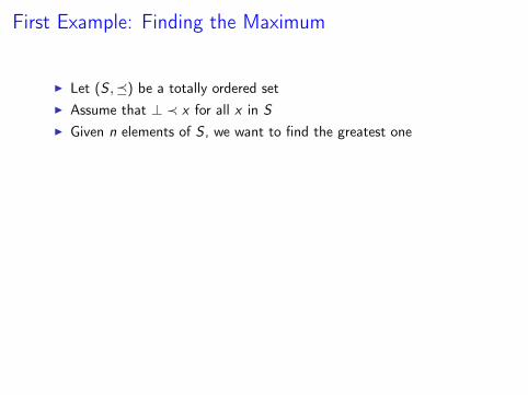
First Example: Finding the Maximum
I Let (S ,) be a totally ordered set
I Assume that ⊥ ≺ x for all x in SI Given n elements of S , we want to find the greatest one
Algorithm:Input : Integer n ≥ 0, array a = 〈a[1] . . . , a[n]〉 of elements of (S ,)Output: maxa[i ] | i ∈ 1, . . . , nmax← ⊥;for i ← 1 to n do
if a[i ] max thenmax← a[i ];
endendreturn max;How fast is the above algorithm?

First Example: Finding the Maximum
I Let (S ,) be a totally ordered setI Assume that ⊥ ≺ x for all x in S
I Given n elements of S , we want to find the greatest one
Algorithm:Input : Integer n ≥ 0, array a = 〈a[1] . . . , a[n]〉 of elements of (S ,)Output: maxa[i ] | i ∈ 1, . . . , nmax← ⊥;for i ← 1 to n do
if a[i ] max thenmax← a[i ];
endendreturn max;How fast is the above algorithm?
First Example: Finding the Maximum
I Let (S ,) be a totally ordered setI Assume that ⊥ ≺ x for all x in SI Given n elements of S , we want to find the greatest one
Algorithm:Input : Integer n ≥ 0, array a = 〈a[1] . . . , a[n]〉 of elements of (S ,)Output: maxa[i ] | i ∈ 1, . . . , nmax← ⊥;for i ← 1 to n do
if a[i ] max thenmax← a[i ];
endendreturn max;How fast is the above algorithm?

First Example: Finding the Maximum
I Let (S ,) be a totally ordered setI Assume that ⊥ ≺ x for all x in SI Given n elements of S , we want to find the greatest one
Algorithm:
Input : Integer n ≥ 0, array a = 〈a[1] . . . , a[n]〉 of elements of (S ,)Output: maxa[i ] | i ∈ 1, . . . , nmax← ⊥;for i ← 1 to n do
if a[i ] max thenmax← a[i ];
endendreturn max;How fast is the above algorithm?

First Example: Finding the Maximum
I Let (S ,) be a totally ordered setI Assume that ⊥ ≺ x for all x in SI Given n elements of S , we want to find the greatest one
Algorithm:Input : Integer n ≥ 0, array a = 〈a[1] . . . , a[n]〉 of elements of (S ,)Output: maxa[i ] | i ∈ 1, . . . , nmax← ⊥;for i ← 1 to n do
if a[i ] max thenmax← a[i ];
endendreturn max;
How fast is the above algorithm?

First Example: Finding the Maximum
I Let (S ,) be a totally ordered setI Assume that ⊥ ≺ x for all x in SI Given n elements of S , we want to find the greatest one
Algorithm:Input : Integer n ≥ 0, array a = 〈a[1] . . . , a[n]〉 of elements of (S ,)Output: maxa[i ] | i ∈ 1, . . . , nmax← ⊥;for i ← 1 to n do
if a[i ] max thenmax← a[i ];
endendreturn max;How fast is the above algorithm?

Time Complexity of an Algorithm
Algorithm:Input : Integer n ≥ 0, array a = 〈a[1] . . . , a[n]〉 of elements of (S ,)Output: maxa[i ] | i ∈ 1, . . . , nmax← ⊥;for i ← 1 to n do
if a[i ] max thenmax← a[i ];
endendreturn max;
I How many elementary operations on an input of a given size?I Size of the input can be measured by nI Elementary operations: perhaps x ← y and if y x then x ← y . . .I Exactly n + 1 elementary operations on each input of size n

Time Complexity of an Algorithm
Algorithm:Input : Integer n ≥ 0, array a = 〈a[1] . . . , a[n]〉 of elements of (S ,)Output: maxa[i ] | i ∈ 1, . . . , nmax← ⊥;for i ← 1 to n do
if a[i ] max thenmax← a[i ];
endendreturn max;
I How many elementary operations on an input of a given size?
I Size of the input can be measured by nI Elementary operations: perhaps x ← y and if y x then x ← y . . .I Exactly n + 1 elementary operations on each input of size n

Time Complexity of an Algorithm
Algorithm:Input : Integer n ≥ 0, array a = 〈a[1] . . . , a[n]〉 of elements of (S ,)Output: maxa[i ] | i ∈ 1, . . . , nmax← ⊥;for i ← 1 to n do
if a[i ] max thenmax← a[i ];
endendreturn max;
I How many elementary operations on an input of a given size?I Size of the input can be measured by n
I Elementary operations: perhaps x ← y and if y x then x ← y . . .I Exactly n + 1 elementary operations on each input of size n

Time Complexity of an Algorithm
Algorithm:Input : Integer n ≥ 0, array a = 〈a[1] . . . , a[n]〉 of elements of (S ,)Output: maxa[i ] | i ∈ 1, . . . , nmax← ⊥;for i ← 1 to n do
if a[i ] max thenmax← a[i ];
endendreturn max;
I How many elementary operations on an input of a given size?I Size of the input can be measured by nI Elementary operations: perhaps x ← y and if y x then x ← y . . .
I Exactly n + 1 elementary operations on each input of size n

Time Complexity of an Algorithm
Algorithm:Input : Integer n ≥ 0, array a = 〈a[1] . . . , a[n]〉 of elements of (S ,)Output: maxa[i ] | i ∈ 1, . . . , nmax← ⊥;for i ← 1 to n do
if a[i ] max thenmax← a[i ];
endendreturn max;
I How many elementary operations on an input of a given size?I Size of the input can be measured by nI Elementary operations: perhaps x ← y and if y x then x ← y . . .I Exactly n + 1 elementary operations on each input of size n

Time Complexity of an Algorithm
Algorithm:Input : Integer n ≥ 0, array a = 〈a[1] . . . , a[n]〉 of elements of (S ,)Output: maxa[i ] | i ∈ 1, . . . , nmax← ⊥;for i ← 1 to n do
if a[i ] max thenmax← a[i ];
endendreturn max;
I What about elementary “operations” x ← y and x y?I Worst case: 2n + 1 operations on input of size nI Best case: n + 2 operations on input of size nI Or 3n + 1 and 2n + 2???I Does not really matter, in each case the number is linear in nI Time complexity can only be given with respect to some underlying
model (e.g., set of elementary operations)

Time Complexity of an Algorithm
Algorithm:Input : Integer n ≥ 0, array a = 〈a[1] . . . , a[n]〉 of elements of (S ,)Output: maxa[i ] | i ∈ 1, . . . , nmax← ⊥;for i ← 1 to n do
if a[i ] max thenmax← a[i ];
endendreturn max;
I What about elementary “operations” x ← y and x y?
I Worst case: 2n + 1 operations on input of size nI Best case: n + 2 operations on input of size nI Or 3n + 1 and 2n + 2???I Does not really matter, in each case the number is linear in nI Time complexity can only be given with respect to some underlying
model (e.g., set of elementary operations)

Time Complexity of an Algorithm
Algorithm:Input : Integer n ≥ 0, array a = 〈a[1] . . . , a[n]〉 of elements of (S ,)Output: maxa[i ] | i ∈ 1, . . . , nmax← ⊥;for i ← 1 to n do
if a[i ] max thenmax← a[i ];
endendreturn max;
I What about elementary “operations” x ← y and x y?I Worst case: 2n + 1 operations on input of size n
I Best case: n + 2 operations on input of size nI Or 3n + 1 and 2n + 2???I Does not really matter, in each case the number is linear in nI Time complexity can only be given with respect to some underlying
model (e.g., set of elementary operations)

Time Complexity of an Algorithm
Algorithm:Input : Integer n ≥ 0, array a = 〈a[1] . . . , a[n]〉 of elements of (S ,)Output: maxa[i ] | i ∈ 1, . . . , nmax← ⊥;for i ← 1 to n do
if a[i ] max thenmax← a[i ];
endendreturn max;
I What about elementary “operations” x ← y and x y?I Worst case: 2n + 1 operations on input of size nI Best case: n + 2 operations on input of size n
I Or 3n + 1 and 2n + 2???I Does not really matter, in each case the number is linear in nI Time complexity can only be given with respect to some underlying
model (e.g., set of elementary operations)

Time Complexity of an Algorithm
Algorithm:Input : Integer n ≥ 0, array a = 〈a[1] . . . , a[n]〉 of elements of (S ,)Output: maxa[i ] | i ∈ 1, . . . , nmax← ⊥;for i ← 1 to n do
if a[i ] max thenmax← a[i ];
endendreturn max;
I What about elementary “operations” x ← y and x y?I Worst case: 2n + 1 operations on input of size nI Best case: n + 2 operations on input of size nI Or 3n + 1 and 2n + 2???
I Does not really matter, in each case the number is linear in nI Time complexity can only be given with respect to some underlying
model (e.g., set of elementary operations)

Time Complexity of an Algorithm
Algorithm:Input : Integer n ≥ 0, array a = 〈a[1] . . . , a[n]〉 of elements of (S ,)Output: maxa[i ] | i ∈ 1, . . . , nmax← ⊥;for i ← 1 to n do
if a[i ] max thenmax← a[i ];
endendreturn max;
I What about elementary “operations” x ← y and x y?I Worst case: 2n + 1 operations on input of size nI Best case: n + 2 operations on input of size nI Or 3n + 1 and 2n + 2???I Does not really matter, in each case the number is linear in n
I Time complexity can only be given with respect to some underlyingmodel (e.g., set of elementary operations)

Time Complexity of an Algorithm
Algorithm:Input : Integer n ≥ 0, array a = 〈a[1] . . . , a[n]〉 of elements of (S ,)Output: maxa[i ] | i ∈ 1, . . . , nmax← ⊥;for i ← 1 to n do
if a[i ] max thenmax← a[i ];
endendreturn max;
I What about elementary “operations” x ← y and x y?I Worst case: 2n + 1 operations on input of size nI Best case: n + 2 operations on input of size nI Or 3n + 1 and 2n + 2???I Does not really matter, in each case the number is linear in nI Time complexity can only be given with respect to some underlying
model (e.g., set of elementary operations)

Time Complexity of an Algorithm
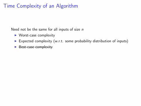
Need not be the same for all inputs of size n
I Worst-case complexityI Expected complexity (w.r.t. some probability distribution of inputs)I Best-case complexity
We have seen that there is an algorithm for finding a maximum in linearworst-case time
I There definitely is an algorithm that is slower in worst caseI And there also might be a substantially faster algorithm. . .I . . . But there is no such algorithm (proof?)

Time Complexity of an Algorithm
Need not be the same for all inputs of size nI Worst-case complexity
I Expected complexity (w.r.t. some probability distribution of inputs)I Best-case complexity
We have seen that there is an algorithm for finding a maximum in linearworst-case time
I There definitely is an algorithm that is slower in worst caseI And there also might be a substantially faster algorithm. . .I . . . But there is no such algorithm (proof?)

Time Complexity of an Algorithm
Need not be the same for all inputs of size nI Worst-case complexityI Expected complexity (w.r.t. some probability distribution of inputs)
I Best-case complexity
We have seen that there is an algorithm for finding a maximum in linearworst-case time
I There definitely is an algorithm that is slower in worst caseI And there also might be a substantially faster algorithm. . .I . . . But there is no such algorithm (proof?)
Time Complexity of an Algorithm
Need not be the same for all inputs of size nI Worst-case complexityI Expected complexity (w.r.t. some probability distribution of inputs)I Best-case complexity
We have seen that there is an algorithm for finding a maximum in linearworst-case time
I There definitely is an algorithm that is slower in worst caseI And there also might be a substantially faster algorithm. . .I . . . But there is no such algorithm (proof?)

Time Complexity of an Algorithm
Need not be the same for all inputs of size nI Worst-case complexityI Expected complexity (w.r.t. some probability distribution of inputs)I Best-case complexity
We have seen that there is an algorithm for finding a maximum in linearworst-case time
I There definitely is an algorithm that is slower in worst case
I And there also might be a substantially faster algorithm. . .I . . . But there is no such algorithm (proof?)

Time Complexity of an Algorithm
Need not be the same for all inputs of size nI Worst-case complexityI Expected complexity (w.r.t. some probability distribution of inputs)I Best-case complexity
We have seen that there is an algorithm for finding a maximum in linearworst-case time
I There definitely is an algorithm that is slower in worst caseI And there also might be a substantially faster algorithm. . .
I . . . But there is no such algorithm (proof?)

Time Complexity of an Algorithm
Need not be the same for all inputs of size nI Worst-case complexityI Expected complexity (w.r.t. some probability distribution of inputs)I Best-case complexity
We have seen that there is an algorithm for finding a maximum in linearworst-case time
I There definitely is an algorithm that is slower in worst caseI And there also might be a substantially faster algorithm. . .I . . . But there is no such algorithm (proof?)

Time Complexity of an Algorithm
Need not be the same for all inputs of size nI Worst-case complexityI Expected complexity (w.r.t. some probability distribution of inputs)I Best-case complexity
We have seen that there is an algorithm for finding a maximum in linearworst-case time
I There definitely is an algorithm that is slower in worst caseI And there also might be a substantially faster algorithm. . .I . . . But there is no such algorithm (proof?)

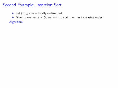
Second Example: Insertion Sort
I Let (S ,) be a totally ordered set
I Given n elements of S , we wish to sort them in increasing orderAlgorithm:Input : Integer n ≥ 0, array a = 〈a[1] . . . , a[n]〉 of elements of (S ,)Behaviour: Sorts a in increasing order
for i ← 2 to n dokey← a[i ];j ← i ;while j ≥ 2 and a[j − 1] key do
A[j ]← A[j − 1];j ← j − 1;
endA[j ]← key
end
I Worst-case time complexity?I It will get much more complicated laterI Seems that we need some techniques that would help us forget
about unimportant details. . .

Second Example: Insertion Sort
I Let (S ,) be a totally ordered setI Given n elements of S , we wish to sort them in increasing order
Algorithm:Input : Integer n ≥ 0, array a = 〈a[1] . . . , a[n]〉 of elements of (S ,)Behaviour: Sorts a in increasing order
for i ← 2 to n dokey← a[i ];j ← i ;while j ≥ 2 and a[j − 1] key do
A[j ]← A[j − 1];j ← j − 1;
endA[j ]← key
end
I Worst-case time complexity?I It will get much more complicated laterI Seems that we need some techniques that would help us forget
about unimportant details. . .
Second Example: Insertion Sort
I Let (S ,) be a totally ordered setI Given n elements of S , we wish to sort them in increasing order
Algorithm:
Input : Integer n ≥ 0, array a = 〈a[1] . . . , a[n]〉 of elements of (S ,)Behaviour: Sorts a in increasing order
for i ← 2 to n dokey← a[i ];j ← i ;while j ≥ 2 and a[j − 1] key do
A[j ]← A[j − 1];j ← j − 1;
endA[j ]← key
end
I Worst-case time complexity?I It will get much more complicated laterI Seems that we need some techniques that would help us forget
about unimportant details. . .

Second Example: Insertion Sort
I Let (S ,) be a totally ordered setI Given n elements of S , we wish to sort them in increasing order
Algorithm:Input : Integer n ≥ 0, array a = 〈a[1] . . . , a[n]〉 of elements of (S ,)Behaviour: Sorts a in increasing order
for i ← 2 to n dokey← a[i ];j ← i ;while j ≥ 2 and a[j − 1] key do
A[j ]← A[j − 1];j ← j − 1;
endA[j ]← key
end
I Worst-case time complexity?I It will get much more complicated laterI Seems that we need some techniques that would help us forget
about unimportant details. . .

Second Example: Insertion Sort
I Let (S ,) be a totally ordered setI Given n elements of S , we wish to sort them in increasing order
Algorithm:Input : Integer n ≥ 0, array a = 〈a[1] . . . , a[n]〉 of elements of (S ,)Behaviour: Sorts a in increasing order
for i ← 2 to n dokey← a[i ];j ← i ;while j ≥ 2 and a[j − 1] key do
A[j ]← A[j − 1];j ← j − 1;
endA[j ]← key
end
I Worst-case time complexity?
I It will get much more complicated laterI Seems that we need some techniques that would help us forget
about unimportant details. . .

Second Example: Insertion Sort
I Let (S ,) be a totally ordered setI Given n elements of S , we wish to sort them in increasing order
Algorithm:Input : Integer n ≥ 0, array a = 〈a[1] . . . , a[n]〉 of elements of (S ,)Behaviour: Sorts a in increasing order
for i ← 2 to n dokey← a[i ];j ← i ;while j ≥ 2 and a[j − 1] key do
A[j ]← A[j − 1];j ← j − 1;
endA[j ]← key
end
I Worst-case time complexity?I It will get much more complicated later
I Seems that we need some techniques that would help us forgetabout unimportant details. . .

Second Example: Insertion Sort
I Let (S ,) be a totally ordered setI Given n elements of S , we wish to sort them in increasing order
Algorithm:Input : Integer n ≥ 0, array a = 〈a[1] . . . , a[n]〉 of elements of (S ,)Behaviour: Sorts a in increasing order
for i ← 2 to n dokey← a[i ];j ← i ;while j ≥ 2 and a[j − 1] key do
A[j ]← A[j − 1];j ← j − 1;
endA[j ]← key
end
I Worst-case time complexity?I It will get much more complicated laterI Seems that we need some techniques that would help us forget
about unimportant details. . .

Motivation for Asymptotic Analysis
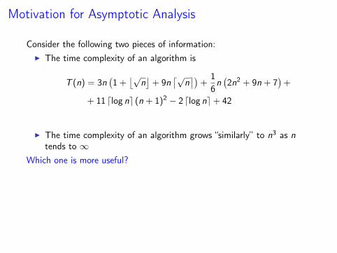
Consider the following two pieces of information:
I The time complexity of an algorithm is
T (n) = 3n(1 +
⌊√n⌋
+ 9n⌈√
n⌉)
+16n(2n2 + 9n + 7
)+
+ 11 dlog ne (n + 1)2 − 2 dlog ne+ 42
I The time complexity of an algorithm grows “similarly” to n3 as ntends to ∞
Which one is more useful?
Exact time complexity is not only hard to compute, but may also be hardto comprehend:
I Solution: asymptotic analysisI We shall be primarily interested in time complexity for large inputsI That is, when n→∞

Motivation for Asymptotic Analysis
Consider the following two pieces of information:I The time complexity of an algorithm is
T (n) = 3n(1 +
⌊√n⌋
+ 9n⌈√
n⌉)
+16n(2n2 + 9n + 7
)+
+ 11 dlog ne (n + 1)2 − 2 dlog ne+ 42
I The time complexity of an algorithm grows “similarly” to n3 as ntends to ∞
Which one is more useful?
Exact time complexity is not only hard to compute, but may also be hardto comprehend:
I Solution: asymptotic analysisI We shall be primarily interested in time complexity for large inputsI That is, when n→∞

Motivation for Asymptotic Analysis
Consider the following two pieces of information:I The time complexity of an algorithm is
T (n) = 3n(1 +
⌊√n⌋
+ 9n⌈√
n⌉)
+16n(2n2 + 9n + 7
)+
+ 11 dlog ne (n + 1)2 − 2 dlog ne+ 42
I The time complexity of an algorithm grows “similarly” to n3 as ntends to ∞
Which one is more useful?
Exact time complexity is not only hard to compute, but may also be hardto comprehend:
I Solution: asymptotic analysis
I We shall be primarily interested in time complexity for large inputsI That is, when n→∞

Motivation for Asymptotic Analysis
Consider the following two pieces of information:I The time complexity of an algorithm is
T (n) = 3n(1 +
⌊√n⌋
+ 9n⌈√
n⌉)
+16n(2n2 + 9n + 7
)+
+ 11 dlog ne (n + 1)2 − 2 dlog ne+ 42
I The time complexity of an algorithm grows “similarly” to n3 as ntends to ∞
Which one is more useful?
Exact time complexity is not only hard to compute, but may also be hardto comprehend:
I Solution: asymptotic analysisI We shall be primarily interested in time complexity for large inputs
I That is, when n→∞

Motivation for Asymptotic Analysis
Consider the following two pieces of information:I The time complexity of an algorithm is
T (n) = 3n(1 +
⌊√n⌋
+ 9n⌈√
n⌉)
+16n(2n2 + 9n + 7
)+
+ 11 dlog ne (n + 1)2 − 2 dlog ne+ 42
I The time complexity of an algorithm grows “similarly” to n3 as ntends to ∞
Which one is more useful?
Exact time complexity is not only hard to compute, but may also be hardto comprehend:
I Solution: asymptotic analysisI We shall be primarily interested in time complexity for large inputsI That is, when n→∞

How Large is This Number? (Think of Money)
4280851899489560848691

And How Large is This Number? (Think of Money)
847955518187334829283589897040119655235863919601693531238414992751617165416141302480796865188930627435280282706613547980294932630735849850955629756390189988065670926936776080112344478419587070503835005599718728588150686533243684009181797426171883222991245962132902198193449147350817134122866534527139324266014275038885469315531344270843365472877851040028341343446812975361588038115962323696276213633010227723117346742793809486832344936918539522695019005474402586729448774658329488313043282804390925188410810300110289559989160868665250433758583040150144399344168406565330785174160961264728256705619645503580555958532651067869506317081480329379589924149250096656021238118034770836265089287436131069459108907243619617600703335393461805670822333994164179926751412897021280473168238505249057658869931528787705337703014030771056967154328101426613199719676876144322924501319536021077133567603615839764872627762350534910009155649512153176581308880648714210251982144207662692294855573895970855089312576731955964946046833813864004631753962686876000391297519828520284626088552126304691777575316106827163895406324359401238410333876306989075934741951911

Asymptotic Analysis
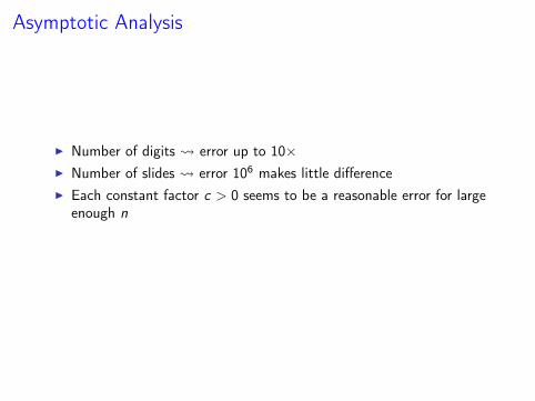
I Number of digits error up to 10×
I Number of slides error 106 makes little differenceI Each constant factor c > 0 seems to be a reasonable error for large
enough nI We shall say that f : N→ N grows “similarly” to g : N→ N if there
is such constant factor c

Asymptotic Analysis
I Number of digits error up to 10×I Number of slides error 106 makes little difference
I Each constant factor c > 0 seems to be a reasonable error for largeenough n
I We shall say that f : N→ N grows “similarly” to g : N→ N if thereis such constant factor c
Asymptotic Analysis
I Number of digits error up to 10×I Number of slides error 106 makes little differenceI Each constant factor c > 0 seems to be a reasonable error for large
enough n
I We shall say that f : N→ N grows “similarly” to g : N→ N if thereis such constant factor c

Asymptotic Analysis
I Number of digits error up to 10×I Number of slides error 106 makes little differenceI Each constant factor c > 0 seems to be a reasonable error for large
enough nI We shall say that f : N→ N grows “similarly” to g : N→ N if there
is such constant factor c

Asymptotic Analysis
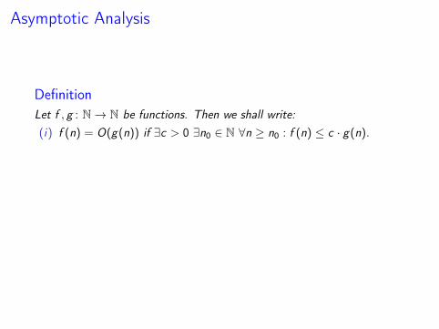
DefinitionLet f , g : N→ N be functions. Then we shall write:
(i) f (n) = O(g(n)) if ∃c > 0 ∃n0 ∈ N ∀n ≥ n0 : f (n) ≤ c · g(n).(ii) f (n) = Ω(g(n)) if g(n) = O(f (n)).(iii) f (n) = Θ(g(n)) if f (n) = O(g(n)) and g(n) = O(f (n)).Some stronger notation:
(iv) f (n) = o(g(n)) if limn→∞f (n)g(n) = 0.
(v) f (n) = ω(g(n)) if g(n) = o(f (n)).
(vi) f (n) ∼ g(n) if limn→∞f (n)g(n) = 1.
Asymptotic Analysis
DefinitionLet f , g : N→ N be functions. Then we shall write:(i) f (n) = O(g(n)) if ∃c > 0 ∃n0 ∈ N ∀n ≥ n0 : f (n) ≤ c · g(n).
(ii) f (n) = Ω(g(n)) if g(n) = O(f (n)).(iii) f (n) = Θ(g(n)) if f (n) = O(g(n)) and g(n) = O(f (n)).Some stronger notation:
(iv) f (n) = o(g(n)) if limn→∞f (n)g(n) = 0.
(v) f (n) = ω(g(n)) if g(n) = o(f (n)).
(vi) f (n) ∼ g(n) if limn→∞f (n)g(n) = 1.

Asymptotic Analysis
DefinitionLet f , g : N→ N be functions. Then we shall write:(i) f (n) = O(g(n)) if ∃c > 0 ∃n0 ∈ N ∀n ≥ n0 : f (n) ≤ c · g(n).(ii) f (n) = Ω(g(n)) if g(n) = O(f (n)).
(iii) f (n) = Θ(g(n)) if f (n) = O(g(n)) and g(n) = O(f (n)).Some stronger notation:
(iv) f (n) = o(g(n)) if limn→∞f (n)g(n) = 0.
(v) f (n) = ω(g(n)) if g(n) = o(f (n)).
(vi) f (n) ∼ g(n) if limn→∞f (n)g(n) = 1.

Asymptotic Analysis
DefinitionLet f , g : N→ N be functions. Then we shall write:(i) f (n) = O(g(n)) if ∃c > 0 ∃n0 ∈ N ∀n ≥ n0 : f (n) ≤ c · g(n).(ii) f (n) = Ω(g(n)) if g(n) = O(f (n)).(iii) f (n) = Θ(g(n)) if f (n) = O(g(n)) and g(n) = O(f (n)).
Some stronger notation:
(iv) f (n) = o(g(n)) if limn→∞f (n)g(n) = 0.
(v) f (n) = ω(g(n)) if g(n) = o(f (n)).
(vi) f (n) ∼ g(n) if limn→∞f (n)g(n) = 1.

Asymptotic Analysis
DefinitionLet f , g : N→ N be functions. Then we shall write:(i) f (n) = O(g(n)) if ∃c > 0 ∃n0 ∈ N ∀n ≥ n0 : f (n) ≤ c · g(n).(ii) f (n) = Ω(g(n)) if g(n) = O(f (n)).(iii) f (n) = Θ(g(n)) if f (n) = O(g(n)) and g(n) = O(f (n)).Some stronger notation:
(iv) f (n) = o(g(n)) if limn→∞f (n)g(n) = 0.
(v) f (n) = ω(g(n)) if g(n) = o(f (n)).
(vi) f (n) ∼ g(n) if limn→∞f (n)g(n) = 1.

Asymptotic Analysis
Example
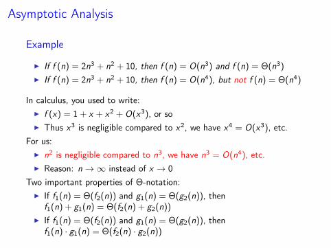
I If f (n) = 2n3 + n2 + 10, then f (n) = O(n3) and f (n) = Θ(n3)
I If f (n) = 2n3 + n2 + 10, then f (n) = O(n4), but not f (n) = Θ(n4)
In calculus, you used to write:I f (x) = 1 + x + x2 + O(x3), or soI Thus x3 is negligible compared to x2, we have x4 = O(x3), etc.
For us:I n2 is negligible compared to n3, we have n3 = O(n4), etc.I Reason: n→∞ instead of x → 0
Two important properties of Θ-notation:I If f1(n) = Θ(f2(n)) and g1(n) = Θ(g2(n)), then
f1(n) + g1(n) = Θ(f2(n) + g2(n))
I If f1(n) = Θ(f2(n)) and g1(n) = Θ(g2(n)), thenf1(n) · g1(n) = Θ(f2(n) · g2(n))

Asymptotic Analysis
Example
I If f (n) = 2n3 + n2 + 10, then f (n) = O(n3) and f (n) = Θ(n3)
I If f (n) = 2n3 + n2 + 10, then f (n) = O(n4), but not f (n) = Θ(n4)
In calculus, you used to write:
I f (x) = 1 + x + x2 + O(x3), or soI Thus x3 is negligible compared to x2, we have x4 = O(x3), etc.
For us:I n2 is negligible compared to n3, we have n3 = O(n4), etc.I Reason: n→∞ instead of x → 0
Two important properties of Θ-notation:I If f1(n) = Θ(f2(n)) and g1(n) = Θ(g2(n)), then
f1(n) + g1(n) = Θ(f2(n) + g2(n))
I If f1(n) = Θ(f2(n)) and g1(n) = Θ(g2(n)), thenf1(n) · g1(n) = Θ(f2(n) · g2(n))

Asymptotic Analysis
Example
I If f (n) = 2n3 + n2 + 10, then f (n) = O(n3) and f (n) = Θ(n3)
I If f (n) = 2n3 + n2 + 10, then f (n) = O(n4), but not f (n) = Θ(n4)
In calculus, you used to write:I f (x) = 1 + x + x2 + O(x3), or so
I Thus x3 is negligible compared to x2, we have x4 = O(x3), etc.For us:
I n2 is negligible compared to n3, we have n3 = O(n4), etc.I Reason: n→∞ instead of x → 0
Two important properties of Θ-notation:I If f1(n) = Θ(f2(n)) and g1(n) = Θ(g2(n)), then
f1(n) + g1(n) = Θ(f2(n) + g2(n))
I If f1(n) = Θ(f2(n)) and g1(n) = Θ(g2(n)), thenf1(n) · g1(n) = Θ(f2(n) · g2(n))

Asymptotic Analysis
Example
I If f (n) = 2n3 + n2 + 10, then f (n) = O(n3) and f (n) = Θ(n3)
I If f (n) = 2n3 + n2 + 10, then f (n) = O(n4), but not f (n) = Θ(n4)
In calculus, you used to write:I f (x) = 1 + x + x2 + O(x3), or soI Thus x3 is negligible compared to x2, we have x4 = O(x3), etc.
For us:I n2 is negligible compared to n3, we have n3 = O(n4), etc.I Reason: n→∞ instead of x → 0
Two important properties of Θ-notation:I If f1(n) = Θ(f2(n)) and g1(n) = Θ(g2(n)), then
f1(n) + g1(n) = Θ(f2(n) + g2(n))
I If f1(n) = Θ(f2(n)) and g1(n) = Θ(g2(n)), thenf1(n) · g1(n) = Θ(f2(n) · g2(n))

Asymptotic Analysis
Example
I If f (n) = 2n3 + n2 + 10, then f (n) = O(n3) and f (n) = Θ(n3)
I If f (n) = 2n3 + n2 + 10, then f (n) = O(n4), but not f (n) = Θ(n4)
In calculus, you used to write:I f (x) = 1 + x + x2 + O(x3), or soI Thus x3 is negligible compared to x2, we have x4 = O(x3), etc.
For us:
I n2 is negligible compared to n3, we have n3 = O(n4), etc.I Reason: n→∞ instead of x → 0
Two important properties of Θ-notation:I If f1(n) = Θ(f2(n)) and g1(n) = Θ(g2(n)), then
f1(n) + g1(n) = Θ(f2(n) + g2(n))
I If f1(n) = Θ(f2(n)) and g1(n) = Θ(g2(n)), thenf1(n) · g1(n) = Θ(f2(n) · g2(n))

Asymptotic Analysis
Example
I If f (n) = 2n3 + n2 + 10, then f (n) = O(n3) and f (n) = Θ(n3)
I If f (n) = 2n3 + n2 + 10, then f (n) = O(n4), but not f (n) = Θ(n4)
In calculus, you used to write:I f (x) = 1 + x + x2 + O(x3), or soI Thus x3 is negligible compared to x2, we have x4 = O(x3), etc.
For us:I n2 is negligible compared to n3, we have n3 = O(n4), etc.
I Reason: n→∞ instead of x → 0Two important properties of Θ-notation:
I If f1(n) = Θ(f2(n)) and g1(n) = Θ(g2(n)), thenf1(n) + g1(n) = Θ(f2(n) + g2(n))
I If f1(n) = Θ(f2(n)) and g1(n) = Θ(g2(n)), thenf1(n) · g1(n) = Θ(f2(n) · g2(n))

Asymptotic Analysis
Example
I If f (n) = 2n3 + n2 + 10, then f (n) = O(n3) and f (n) = Θ(n3)
I If f (n) = 2n3 + n2 + 10, then f (n) = O(n4), but not f (n) = Θ(n4)
In calculus, you used to write:I f (x) = 1 + x + x2 + O(x3), or soI Thus x3 is negligible compared to x2, we have x4 = O(x3), etc.
For us:I n2 is negligible compared to n3, we have n3 = O(n4), etc.I Reason: n→∞ instead of x → 0
Two important properties of Θ-notation:I If f1(n) = Θ(f2(n)) and g1(n) = Θ(g2(n)), then
f1(n) + g1(n) = Θ(f2(n) + g2(n))
I If f1(n) = Θ(f2(n)) and g1(n) = Θ(g2(n)), thenf1(n) · g1(n) = Θ(f2(n) · g2(n))

Asymptotic Analysis
Example
I If f (n) = 2n3 + n2 + 10, then f (n) = O(n3) and f (n) = Θ(n3)
I If f (n) = 2n3 + n2 + 10, then f (n) = O(n4), but not f (n) = Θ(n4)
In calculus, you used to write:I f (x) = 1 + x + x2 + O(x3), or soI Thus x3 is negligible compared to x2, we have x4 = O(x3), etc.
For us:I n2 is negligible compared to n3, we have n3 = O(n4), etc.I Reason: n→∞ instead of x → 0
Two important properties of Θ-notation:
I If f1(n) = Θ(f2(n)) and g1(n) = Θ(g2(n)), thenf1(n) + g1(n) = Θ(f2(n) + g2(n))
I If f1(n) = Θ(f2(n)) and g1(n) = Θ(g2(n)), thenf1(n) · g1(n) = Θ(f2(n) · g2(n))

Asymptotic Analysis
Example
I If f (n) = 2n3 + n2 + 10, then f (n) = O(n3) and f (n) = Θ(n3)
I If f (n) = 2n3 + n2 + 10, then f (n) = O(n4), but not f (n) = Θ(n4)
In calculus, you used to write:I f (x) = 1 + x + x2 + O(x3), or soI Thus x3 is negligible compared to x2, we have x4 = O(x3), etc.
For us:I n2 is negligible compared to n3, we have n3 = O(n4), etc.I Reason: n→∞ instead of x → 0
Two important properties of Θ-notation:I If f1(n) = Θ(f2(n)) and g1(n) = Θ(g2(n)), then
f1(n) + g1(n) = Θ(f2(n) + g2(n))
I If f1(n) = Θ(f2(n)) and g1(n) = Θ(g2(n)), thenf1(n) · g1(n) = Θ(f2(n) · g2(n))
Insertion Sort: Worst-Case Time Complexity
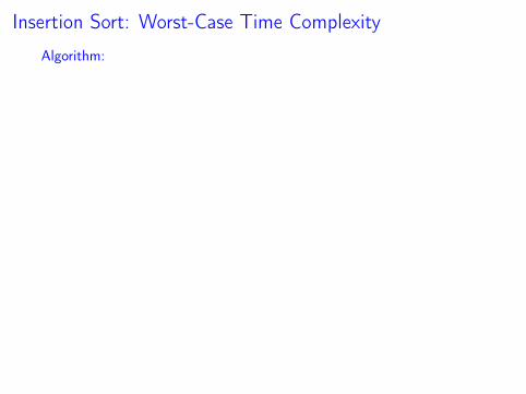
Algorithm:
Input : Integer n ≥ 0, array a = 〈a[1] . . . , a[n]〉 of elements of (S ,)Behaviour: Sorts a in increasing order
for i ← 2 to n dokey← a[i ];j ← i ;while j ≥ 2 and a[j − 1] key do
A[j ]← A[j − 1];j ← j − 1;
endA[j ]← key
end
I Let T (n) be the worst-case time complexity of insertion sortI The for loop executes ≤ n times on each inputI The while loop executes ≤ n times for each iI Hence, T (n) = O(n2)I Considering inputs sorted in decreasing order: T (n) = Ω(n2)I T (n) = Θ(n2)

Insertion Sort: Worst-Case Time Complexity
Algorithm:Input : Integer n ≥ 0, array a = 〈a[1] . . . , a[n]〉 of elements of (S ,)Behaviour: Sorts a in increasing order
for i ← 2 to n dokey← a[i ];j ← i ;while j ≥ 2 and a[j − 1] key do
A[j ]← A[j − 1];j ← j − 1;
endA[j ]← key
end
I Let T (n) be the worst-case time complexity of insertion sort
I The for loop executes ≤ n times on each inputI The while loop executes ≤ n times for each iI Hence, T (n) = O(n2)I Considering inputs sorted in decreasing order: T (n) = Ω(n2)I T (n) = Θ(n2)

Insertion Sort: Worst-Case Time Complexity
Algorithm:Input : Integer n ≥ 0, array a = 〈a[1] . . . , a[n]〉 of elements of (S ,)Behaviour: Sorts a in increasing order
for i ← 2 to n dokey← a[i ];j ← i ;while j ≥ 2 and a[j − 1] key do
A[j ]← A[j − 1];j ← j − 1;
endA[j ]← key
end
I Let T (n) be the worst-case time complexity of insertion sortI The for loop executes ≤ n times on each input
I The while loop executes ≤ n times for each iI Hence, T (n) = O(n2)I Considering inputs sorted in decreasing order: T (n) = Ω(n2)I T (n) = Θ(n2)

Insertion Sort: Worst-Case Time Complexity
Algorithm:Input : Integer n ≥ 0, array a = 〈a[1] . . . , a[n]〉 of elements of (S ,)Behaviour: Sorts a in increasing order
for i ← 2 to n dokey← a[i ];j ← i ;while j ≥ 2 and a[j − 1] key do
A[j ]← A[j − 1];j ← j − 1;
endA[j ]← key
end
I Let T (n) be the worst-case time complexity of insertion sortI The for loop executes ≤ n times on each inputI The while loop executes ≤ n times for each i
I Hence, T (n) = O(n2)I Considering inputs sorted in decreasing order: T (n) = Ω(n2)I T (n) = Θ(n2)

Insertion Sort: Worst-Case Time Complexity
Algorithm:Input : Integer n ≥ 0, array a = 〈a[1] . . . , a[n]〉 of elements of (S ,)Behaviour: Sorts a in increasing order
for i ← 2 to n dokey← a[i ];j ← i ;while j ≥ 2 and a[j − 1] key do
A[j ]← A[j − 1];j ← j − 1;
endA[j ]← key
end
I Let T (n) be the worst-case time complexity of insertion sortI The for loop executes ≤ n times on each inputI The while loop executes ≤ n times for each iI Hence, T (n) = O(n2)
I Considering inputs sorted in decreasing order: T (n) = Ω(n2)I T (n) = Θ(n2)

Insertion Sort: Worst-Case Time Complexity
Algorithm:Input : Integer n ≥ 0, array a = 〈a[1] . . . , a[n]〉 of elements of (S ,)Behaviour: Sorts a in increasing order
for i ← 2 to n dokey← a[i ];j ← i ;while j ≥ 2 and a[j − 1] key do
A[j ]← A[j − 1];j ← j − 1;
endA[j ]← key
end
I Let T (n) be the worst-case time complexity of insertion sortI The for loop executes ≤ n times on each inputI The while loop executes ≤ n times for each iI Hence, T (n) = O(n2)I Considering inputs sorted in decreasing order: T (n) = Ω(n2)
I T (n) = Θ(n2)

Insertion Sort: Worst-Case Time Complexity
Algorithm:Input : Integer n ≥ 0, array a = 〈a[1] . . . , a[n]〉 of elements of (S ,)Behaviour: Sorts a in increasing order
for i ← 2 to n dokey← a[i ];j ← i ;while j ≥ 2 and a[j − 1] key do
A[j ]← A[j − 1];j ← j − 1;
endA[j ]← key
end
I Let T (n) be the worst-case time complexity of insertion sortI The for loop executes ≤ n times on each inputI The while loop executes ≤ n times for each iI Hence, T (n) = O(n2)I Considering inputs sorted in decreasing order: T (n) = Ω(n2)I T (n) = Θ(n2)

When Model Matters. . .
Algorithm:
Input : Integer n ≥ 0Output: nn
k ← 1;for i ← 1 to n do
k ← k · n;endreturn k ;
I Worst-case time complexity: Θ(n)?I nn = 2n log n – we need at least n log n bits to store nn
I At least n log n bit operations, and this is not Θ(n)
I Even worse if we take log n as the size of the input

When Model Matters. . .
Algorithm:Input : Integer n ≥ 0Output: nn
k ← 1;for i ← 1 to n do
k ← k · n;endreturn k ;
I Worst-case time complexity: Θ(n)?
I nn = 2n log n – we need at least n log n bits to store nn
I At least n log n bit operations, and this is not Θ(n)
I Even worse if we take log n as the size of the input

When Model Matters. . .
Algorithm:Input : Integer n ≥ 0Output: nn
k ← 1;for i ← 1 to n do
k ← k · n;endreturn k ;
I Worst-case time complexity: Θ(n)?I nn = 2n log n – we need at least n log n bits to store nn
I At least n log n bit operations, and this is not Θ(n)
I Even worse if we take log n as the size of the input

When Model Matters. . .
Algorithm:Input : Integer n ≥ 0Output: nn
k ← 1;for i ← 1 to n do
k ← k · n;endreturn k ;
I Worst-case time complexity: Θ(n)?I nn = 2n log n – we need at least n log n bits to store nn
I At least n log n bit operations, and this is not Θ(n)
I Even worse if we take log n as the size of the input