algorithmic game theory and applications lecture 7: the lp

Algorithmic Game Theory

and Applications

Lecture 7:

The LP Duality Theorem

Kousha Etessami

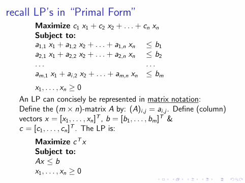
recall LP’s in “Primal Form”Maximize c1 x1 + c2 x2 + . . . + cn xn

Subject to:a1,1 x1 + a1,2 x2 + . . . + a1,n xn ≤ b1

a2,1 x1 + a2,2 x2 + . . . + a2,n xn ≤ b2

. . . . . .am,1 x1 + ai ,2 x2 + . . . + am,n xn ≤ bm

x1, . . . , xn ≥ 0

An LP can concisely be represented in matrix notation:Define the (m× n)-matrix A by: (A)i ,j = ai ,j . Define (column)vectors x = [x1, . . . , xn]T , b = [b1, . . . , bm]T &c = [c1, . . . , cn]T . The LP is:

Maximize cTxSubject to:Ax ≤ bx1, . . . , xn ≥ 0

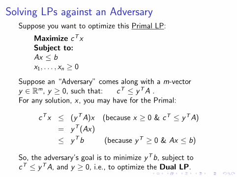
Solving LPs against an AdversarySuppose you want to optimize this Primal LP:


Suppose an “Adversary” comes along with a m-vectory ∈ Rm, y ≥ 0, such that: cT ≤ yTA .For any solution, x , you may have for the Primal:

cTx ≤ (yTA)x (because x ≥ 0 & cT ≤ yTA)

= yT (Ax)

≤ yTb (because yT ≥ 0 & Ax ≤ b)

So, the adversary’s goal is to minimize yTb, subject tocT ≤ yTA, and y ≥ 0, i.e., to optimize the Dual LP.

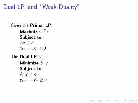
Dual LP, and “Weak Duality”

Given the Primal LP:


The Dual LP is:

Minimize bTySubject to:ATy ≥ cy1, . . . , ym ≥ 0

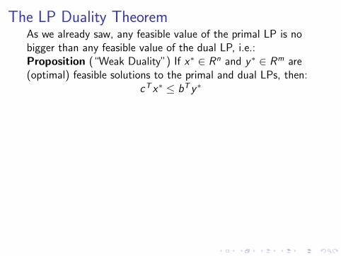
The LP Duality TheoremAs we already saw, any feasible value of the primal LP is nobigger than any feasible value of the dual LP, i.e.:Proposition (“Weak Duality”) If x∗ ∈ Rn and y ∗ ∈ Rm are(optimal) feasible solutions to the primal and dual LPs, then:

cTx∗ ≤ bTy ∗

Amazingly, when x∗ and y ∗ are optimal, equality holds!

Theorem(“Strong Duality”, von Neumann’47) One of thefollowing four situations holds:

1. Both the primal and dual LPs are feasible, and for anyoptimal solutions x∗ of the primal and y ∗ of the dual:

cTx∗ = bTy ∗

2. The primal is infeasible and the dual is unbounded.

3. The primal is unbounded and the dual is infeasible.

4. Both LPs are infeasible.

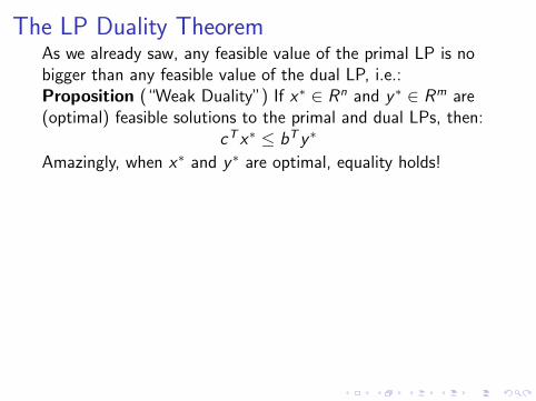
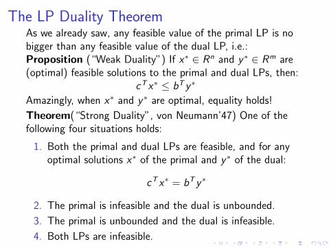
Simplex and the Duality Theorem

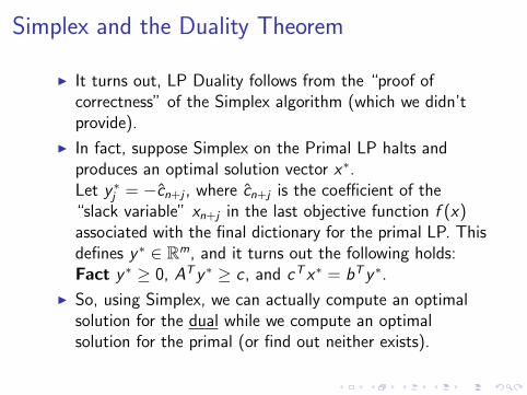
I It turns out, LP Duality follows from the “proof ofcorrectness” of the Simplex algorithm (which we didn’tprovide).

I In fact, suppose Simplex on the Primal LP halts andproduces an optimal solution vector x∗.Let y ∗

j = −cn+j , where cn+j is the coefficient of the“slack variable” xn+j in the last objective function f (x)associated with the final dictionary for the primal LP. Thisdefines y ∗ ∈ Rm, and it turns out the following holds:Fact y ∗ ≥ 0, ATy ∗ ≥ c , and cTx∗ = bTy ∗.

I So, using Simplex, we can actually compute an optimalsolution for the dual while we compute an optimalsolution for the primal (or find out neither exists).

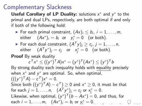
Complementary SlacknessUseful Corollary of LP Duality: solutions x∗ and y ∗ to theprimal and dual LPs, respectively, are both optimal if and onlyif both of the following hold:

I For each primal constraint, (Ax)i ≤ bi , i = 1, . . . , m,either (Ax∗)i = bi or y ∗

i = 0 (or both).

I For each dual constraint, (ATy)j ≥ cj , j = 1, . . . , n,either (ATy ∗)j = cj or x∗

j = 0 (or both).

Proof By weak dualitycTx∗ ≤ ((y ∗)TA)x∗ = (y ∗)T (Ax∗) ≤ (y ∗)Tb

By strong duality each inequality holds with equality preciselywhen x∗ and y ∗ are optimal. So, when optimal,(((y ∗)TA)− cT )x∗ = 0.Since both ((y ∗)TA)− cT ) ≥ 0 and x∗ ≥ 0, it must be thatfor each j = 1, . . . , n, (ATy ∗)j = cj or x∗

j = 0.

Likewise, when optimal, (y ∗)T (b − Ax∗) = 0, and thus, foreach i = 1, . . . , m, (Ax∗)i = bi or y ∗

i = 0.

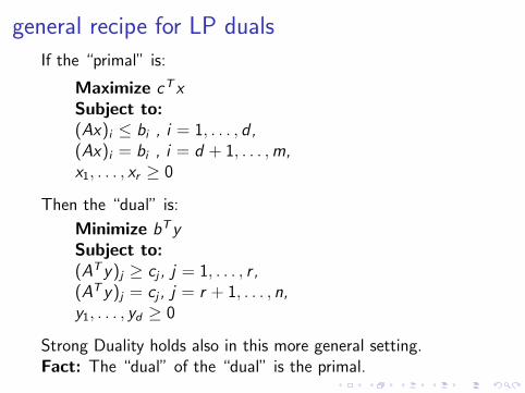
general recipe for LP duals

If the “primal” is:

Maximize cTxSubject to:(Ax)i ≤ bi , i = 1, . . . , d,(Ax)i = bi , i = d + 1, . . . , m,x1, . . . , xr ≥ 0

Then the “dual” is:

Minimize bTySubject to:(ATy)j ≥ cj , j = 1, . . . , r ,(ATy)j = cj , j = r + 1, . . . , n,y1, . . . , yd ≥ 0

Strong Duality holds also in this more general setting.Fact: The “dual” of the “dual” is the primal.

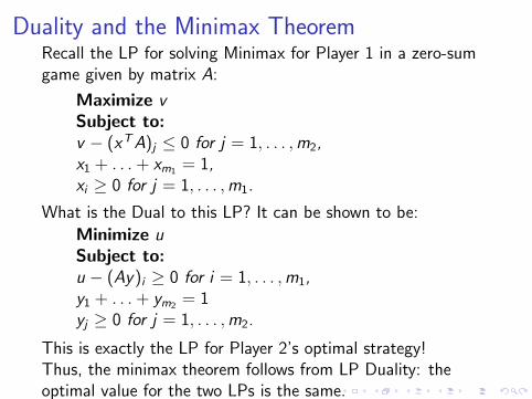
Duality and the Minimax TheoremRecall the LP for solving Minimax for Player 1 in a zero-sumgame given by matrix A:

Maximize vSubject to:v − (xTA)j ≤ 0 for j = 1, . . . , m2,x1 + . . . + xm1 = 1,xi ≥ 0 for j = 1, . . . , m1.

What is the Dual to this LP? It can be shown to be:

Minimize uSubject to:u − (Ay)i ≥ 0 for i = 1, . . . , m1,y1 + . . . + ym2 = 1yj ≥ 0 for j = 1, . . . , m2.

This is exactly the LP for Player 2’s optimal strategy!Thus, the minimax theorem follows from LP Duality: theoptimal value for the two LPs is the same.

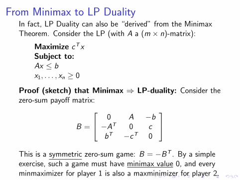
From Minimax to LP DualityIn fact, LP Duality can also be “derived” from the MinimaxTheorem. Consider the LP (with A a (m × n)-matrix):


Proof (sketch) that Minimax ⇒ LP-duality: Consider thezero-sum payoff matrix:

B =

0 A −b−AT 0 cbT −cT 0

This is a symmetric zero-sum game: B = −BT . By a simpleexercise, such a game must have minimax value 0, and everyminmaximizer for player 1 is also a maxminimizer for player 2.

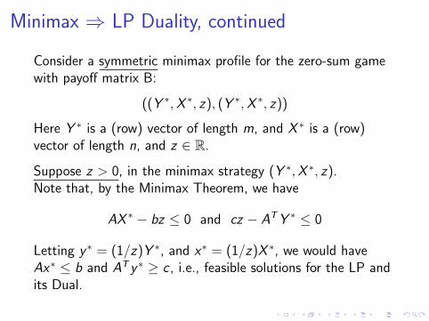
Minimax ⇒ LP Duality, continued

Consider a symmetric minimax profile for the zero-sum gamewith payoff matrix B:

((Y ∗, X ∗, z), (Y ∗, X ∗, z))

Here Y ∗ is a (row) vector of length m, and X ∗ is a (row)vector of length n, and z ∈ R.

Suppose z > 0, in the minimax strategy (Y ∗, X ∗, z).Note that, by the Minimax Theorem, we have

AX ∗ − bz ≤ 0 and cz − ATY ∗ ≤ 0

Letting y ∗ = (1/z)Y ∗, and x∗ = (1/z)X ∗, we would haveAx∗ ≤ b and ATy ∗ ≥ c , i.e., feasible solutions for the LP andits Dual.

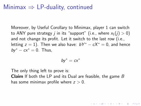
Minimax ⇒ LP-duality, continued

Moreover, by Useful Corollary to Minimax, player 1 can switchto ANY pure strategy j in its “support” (i.e., where x1(j) > 0)and not change its profit. Let it switch to the last row (i.e.,letting z = 1). Then we also have: bY ∗ − cX ∗ = 0, and henceby ∗ − cx∗ = 0. Thus,

by ∗ = cx∗

The only thing left to prove is:Claim If both the LP and its Dual are feasible, the game Bhas some minimax profile where z > 0.

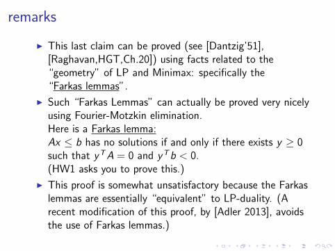
remarks

I This last claim can be proved (see [Dantzig’51],[Raghavan,HGT,Ch.20]) using facts related to the“geometry” of LP and Minimax: specifically the“Farkas lemmas”.

I Such “Farkas Lemmas” can actually be proved very nicelyusing Fourier-Motzkin elimination.Here is a Farkas lemma:Ax ≤ b has no solutions if and only if there exists y ≥ 0such that yTA = 0 and yTb < 0.(HW1 asks you to prove this.)

I This proof is somewhat unsatisfactory because the Farkaslemmas are essentially “equivalent” to LP-duality. (Arecent modification of this proof, by [Adler 2013], avoidsthe use of Farkas lemmas.)

Significance of LP DualityI The Duality Theorem is an extremely important fact. It

has many uses, e.g., in (combinatorial) optimization andmathematical economics.

I Often, you can “learn something” about an LP by lookingat its dual.

I In Economics, one often sets up an LP to optimize someeconomic goal. Often, the dual LP can be meaningfullyinterpreted as a problem of optimizing some realeconomic “counter” goal.The fact that the optimal solutions of the two goals arethe same is very powerful.

I Duality has many consequences in algorithms.For example, duality implies that LPs can be solved in“NP ∩ co-NP”.(Of course, we know from [Khachian’79] that the LPproblem is in “P”.)

more on algorithmic significance(*) approximation algorithms: hard combinatorial optimizationproblems can often be formulated as “Integer Linear Progams”(ILPs). One can often use the “LP-relaxation” of the ILPtogether with its Dual to find approximate solutions and tobound the proximity of the approximate solution to theoptimal. (See, e.g., [Vazirani’2001].)

(*) Many important results in combinatorics can be viewed asparticular manifestations of LP Duality.

I Max-Flow Min-Cut Theorem; Hall’s Theorem;Dilworth’s Theorem; Konig-Egervary Theorem......

Each result says “the maximum value of one useful quantityassociated with a combinatorial object is the same as theminimum value of another useful quantity associated with it.”These follow from LP-Duality: dual LPs for these“complementary” quantities can be set up (with solutions thatconsist necessarily of integers, due to the LPs’ structure).

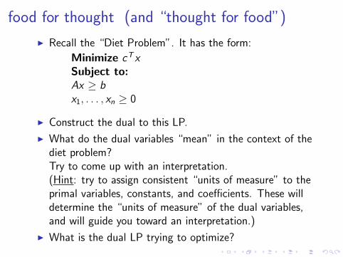
food for thought (and “thought for food”)

I Recall the “Diet Problem”. It has the form:

Minimize cTxSubject to:Ax ≥ bx1, . . . , xn ≥ 0

I Construct the dual to this LP.

I What do the dual variables “mean” in the context of thediet problem?Try to come up with an interpretation.(Hint: try to assign consistent “units of measure” to theprimal variables, constants, and coefficients. These willdetermine the “units of measure” of the dual variables,and will guide you toward an interpretation.)

I What is the dual LP trying to optimize?

algorithmic game theory and applications lecture 7: the lp

Documents