MODIS Leaf Area Index (LAI) And Fraction OfPhotosynthetically Active Radiation Absorbed By Vegetation

(FPAR) Product

(MOD15)

Algorithm Theoretical Basis Document

Version 4.0

R. B. Myneni, Y. Knyazikhin,Y. Zhang, Y. Tian, Y. Wang,A. Lotsch

J. L. Privette,J. T. Morisette

S. W. Running, R. Nemani,J.Glassy, P.Votava

Department of GeographyBoston UniversityBoston, MA 02215rmyneni@crsa.bu.edu

NASA’s Goddard SpaceFlight Centerjeff.privette@gsfc.nasa.gov

School of ForestryUniversity of MontanaMissoula, MT 59812swr@ntsg.umt.edu

Cite as:

Y. Knyazikhin, J. Glassy, J. L. Privette, Y. Tian, A. Lotsch, Y. Zhang, Y. Wang,J. T. Morisette, P.Votava, R.B. Myneni, R. R. Nemani, S. W. Running,MODIS Leaf Area Index (LAI) and Fraction of Photosynthetically Active RadiationAbsorbed by Vegetation (FPAR) Product (MOD15) Algorithm Theoretical BasisDocument, http://eospso.gsfc.nasa.gov/atbd/modistables.html, 1999.

This document was prepared by Y. Zhang

April 30, 1999

Abstract

This Algorithm Theoretical Basis Document (ATBD) describes the algorithm toproduce global Leaf Area Index (LAI) and Fraction of Photosynthetically Active Radiation(FPAR) absorbed by vegetation from atmospherically corrected surface reflectances. TheMOD15 LAI and FPAR products are 1 km at launch products provided on a daily and 8days basis. The algorithm consists of a main procedure that exploits the spectralinformation content of MODIS surface reflectances at up to 7 spectral bands. Should thismain algorithm fail, a back-up algorithm is triggered to estimate LAI and FPAR usingvegetation indices. The algorithm requires a land cover classification that is compatiblewith the radiative transfer model used in their derivation. Such a classification based onvegetation structure was proposed and it is expected to be derived from the MODIS LandCover Product. Therefore the algorithm has interfaces with the MODIS surface reflectanceproduct (MOD09) and the MODIS Land Cover Product (MOD12).

Derivation of various empirical relationships and trends from the LAI and FPARfields is the most likely approach which a potential user of the LAI and FPAR productswill utilize in his investigation. It sets a demand on the retrieval techniques; that is, the LAIand FPAR fields must posses the same statistical properties as if they were derived fromground based measurements. Therefore we perform our retrievals by comparing observedradiances with modeled radiances for a suite of canopy structure and soil patterns thatcovers a range of expected natural conditions. The set of the canopy/soil patterns for whichthe magnitude of the residuals in the comparisons does not exceed uncertainties inobserved radiances is then used to evaluate the distribution of LAI and FPAR values and tospecify the most probable value of desired parameters. The key mathematics behind thistechnique is the measure theory which is used to establish relationships between thesurface reflectances, uncertainties in their retrieval and canopy/soil patterns. This theoryunderlies a precise mathematical definition of the probability distribution function and thusallows us to meet the above formulated demand.

In order to better describe natural variability of vegetation canopies a three-dimensional formulation of the LAI/FPAR inverse problem underlies the algorithm. Byaccounting features specific to the problem of radiative transfer in plant canopies, powerfultechniques in reactor theory (the Green’s function and adjoint formulation of the problem)were utilized to parameterize the radiative field in terms of reflectance properties of thevacuum bounded canopy and ground, as well as to split the three-dimensional radiativetransfer problem into two independent sub-problems, each of which is expressed in termsof three basic components of the energy conservation law: canopy transmittance,reflectance, and absorptance. These components are elements of the look-up table (LUT),and the algorithm interacts only with the elements of the LUT. This provides theindependence of the retrieval algorithm to a particular canopy radiation model. It is

precisely derived that the dependence of canopy transmittance, reflectance, andabsorptance on wavelength is described by a simple function which depends on the uniquepositive eigenvalue of the transport equation. This eigenvalue relates optical properties ofindividual leaves to canopy structure. This facilitates comparison of spectral values of thecanopy reflectances with spectral properties of individual leaves, which is a rather stablecharacteristic of a green leaf. This allows us to fully take advantage of the spectralinformation content of the MODIS instrument.

The algorithm has been prototyped by Land Surface Reflectances (LASUR) andLandsat data. The prototyping results demonstrated its ability to produce global LAI andFPAR fields. The algorithm and the LUT use directly the information on the leaf canopyspectral properties and structural attributes, in stead of NDVI, to retrieve LAI and FPAR.The effects of biome misclassification between clearly distinct biomes on the algorithmcan be evaluated through the Retrieval Index (RI), mean LAI and the histogram of theretrieved LAI distribution. The dependence of the algorithm on spatial resolution isillustrated using coarse and fine resolution data and LUTs.

Validation of the LAI and FPAR products is an important part of algorithmdevelopment and is in progress under the EOS validation plan. As the global validation ofland remote sensing products is complicated by multiple factors, various validationtechniques will be used to develop uncertainty information on EOS land products. Detailedvalidation methods have been proposed for global scale validation.

The important ancillary data set for this algorithm are the radiative transfer modelcompatible structural land cover classification, which divides the global vegetation landcover into six biomes. Efforts have been made to improve this land cover classificationmap from many data sources. Another important ancillary data set is the LUT of thealgorithm, which is derived from both theory and data set of vegetation, soil opticalproperties. Detailed description of the LUT’s structure and its elements is also given in thisdocument.

The MODIS LAI and FPAR Level 3 algorithms were developed jointly by personnelat Boston University and the University of Montana SCF and NASA GSFC. The BostonUniversity team developed the radiative-transfer (R-T) derivative science core logic andthe R-T driven lookup tables comprising the core science, the direct-retrieval lookuptables, and prototype software for exercising the core logic. The University of MontanaSCF team is responsible for developing, testing, and maintaining the EOSDIS Core System(ECS) production version of the software. QA tasks are shared between the twoinstitutions, with the MOD15A1 QA activities conducted at Boston University, and theMOD15A2 QA activities run at University of Montana SCF. Validation is done by bothBU and UMT SCFs in collaboration with Drs. Privette and Morisette at GSFC.

Table of Contents

1. Introduction .......................................................................................................1 1.1 Identification................................................................................................1 1.2 Overview .....................................................................................................12. Algorithm Description.........................................................................................2 2.1 Introduction ...................................................................................................2 2.2 Canopy Structural Types of Global Vegetation ............................................6 2.3 Radiative Transfer Problem for Vegetation Media .....................................11 2.4 Assumptions in Radiation Transfer Process................................................14 2.5 Mathematical Basis of the Algorithm..........................................................19 2.6 Conservative Models ...................................................................................22 2.7 Constraints on Look-Up Table Entries........................................................29 2.8 Description of LAI Retrieval.......................................................................30 2.9 Saturation Domain.......................................................................................39 2.10 Description of FPAR Retrieval .................................................................42 2.11 Theoretical Basis of NDVI-FPAR Relations ............................................44 2.12 Backup Algorithm .....................................................................................463. Algorithm Prototyping.......................................................................................50 3.1 Data Analysis...............................................................................................50 3.2 Prototyping of the Algorithm ......................................................................544. Validation Plan ..................................................................................................72 4.1 Introduction .................................................................................................72 4.2 Approach .....................................................................................................72 4.3 Validation Sites ...........................................................................................73 4.4 Auxiliary Measurements .............................................................................75 4.5 Scaling .........................................................................................................77 4.6 Modland QUick Airborne LookS (MQUALS) ...........................................77 4.7 Data Protocols and Dissemination...............................................................78 4.8 Proposed Validation Tests...........................................................................805. Ancillary Data ...................................................................................................86 5.1 At-launch Land Cover .................................................................................86 5.2 Look-Up Table Structure.............................................................................926. Programming and Procedural Considerations.................................................104 6.1 Programming Issues ..................................................................................104 6.2 Processing Issues.......................................................................................109 6.3 Quality Assurance .....................................................................................112

References ...........................................................................................................121

1

MODIS FPAR AND LAI PRODUCTS ALGORITHMTECHNICAL BASIS DOCUMENT Version 4.1

1. INTRODUCTION

1.1 Identification

Table 1-1: Product ListMODIS Product No. 15 (MOD15)

ParameterNumber

Parameter NameSpatial

ResolutionTemporalResolution

2680 Leaf Area Index (LAI) 1 km Daily, 8 day

5367Fraction of Photosynthetically Active Radiation

absorbed by vegetation (FPAR)1 km Daily, 8 day

1.2 Overview

This document details the algorithm for producing global terrestrial leaf area index (LAI)product, and the related fraction of absorbed photosynthetically active radiation (FPAR) product.LAI defines an important structural property of a plant canopy, the number of equivalent layersof leaves vegetation displays relative to a unit ground area. FPAR measures the proportion ofavailable radiation in the specific photosynthetically active wavelengths of the spectrum 0.4 - 0.7µm that a canopy absorbs. It is non-linearly related to the LAI.

Both LAI and FPAR will be Level 4 MODIS products derived directly from MODISReflectances (MR) and ancillary data on surface characteristics such as Land cover type,background etc. These products will be produced globally at a time frequency defined by theMODIS Reflectances (MR) global compositing period, 8 days. The spatial resolution will beconstrained by the MODIS reflectance dataset, and may be as fine as 250m, or standardized to1km. The 8 day product will be produced by compositing using maximum FPAR.

2

2. ALGORITHM DESCRIPTION

2.1 Introduction

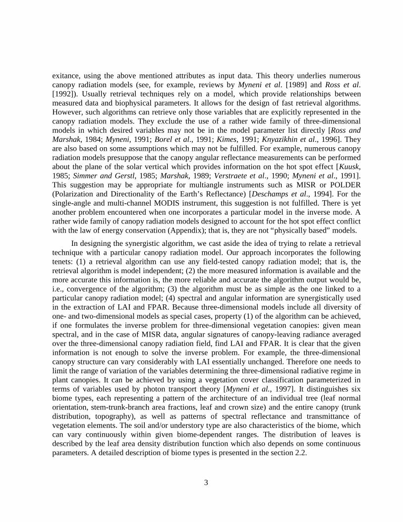
Large-scale ecosystem modeling is used to simulate a range of ecological responses tochanges in climate and chemical composition of the atmosphere, including changes in thedistribution of terrestrial plant communities across the globe in response to climate changes. Leafarea index (LAI) is a state parameter in all models describing the exchange of fluxes of energy,mass (e.g., water and CO2), and momentum between the surface and the planetary boundarylayer. Analyses of global carbon budget indicate a large terrestrial middle- to high-latitude sink,without which the accumulation of carbon in the atmosphere would be higher than the presentrate. The problem of accurately evaluating the exchange of carbon between the atmosphere andthe terrestrial vegetation therefore requires special attention. In this context the fraction ofphotosynthetically active radiation (FPAR) absorbed by global vegetation is a key state variablein most ecosystem productivity models and in global models of climate, hydrology,biogeochemestry, and ecology [Sellers et al., 1997]. Therefore these variables that describevegetation canopy structure and its energy absorption capacity are required by many of the EOSInterdisciplinary Projects [Myneni et al., 1997a]. In order to quantitatively and accurately modelglobal dynamics of these processes, differentiate short-term from long-term trends, as well as todistinguish regional from global phenomena, these two parameters must be collected often for along period of time and should represent every region of the Earth’s lands. Satellite remotesensing serves as the most effective means for collecting global data on a regularly basis. Thelaunch of EOS-AM 1 with MODIS (moderate resolution imaging spectroradiometer) and MISR(multiangle imaging spectroradiometer) instruments onboard begins a new era in remote sensingthe Earth system. In contrast to previous single-angle and single-channel instruments, MODISand MISR together allow for rich spectral and angular sampling of the radiation field reflectedby vegetation canopies. This sets new demands on the retrieval techniques for geophysicalparameters in order to take full advantages of these instruments. Our objective is to derive asynergistic algorithm for the extraction of LAI and FPAR from MODIS- and MISR-measuredcanopy reflectance data, with the flexibility to use the same algorithm in MODIS-only andMISR-only as well. Although a prototyping of the algorithm with data was also a focus of ouractivity, these results are not discussed in this article. Plate 2-1 demonstrates an example of theprototype of the MODIS LAI/FPAR data product.

Solar radiation scattered from a vegetation canopy and measured by satellite sensors resultsfrom interaction of photons traversing through the foliage medium, bounded at the bottom by aradiatively participating surface. Therefore to estimate the canopy radiation regime, threeimportant features must be carefully formulated. They are (1) the architecture of individual plantand the entire canopy; (2) optical properties of vegetation elements (leaves, stems) and soil; theformer depends on physiological conditions (water status, pigment concentration); and (3)atmospheric conditions which determine the incident radiation field. Photon transport theoryaims at deriving the solar radiation regime, both within the vegetation canopy and the radiant

3

exitance, using the above mentioned attributes as input data. This theory underlies numerouscanopy radiation models (see, for example, reviews by Myneni et al. [1989] and Ross et al.[1992]). Usually retrieval techniques rely on a model, which provide relationships betweenmeasured data and biophysical parameters. It allows for the design of fast retrieval algorithms.However, such algorithms can retrieve only those variables that are explicitly represented in thecanopy radiation models. They exclude the use of a rather wide family of three-dimensionalmodels in which desired variables may not be in the model parameter list directly [Ross andMarshak, 1984; Myneni, 1991; Borel et al., 1991; Kimes, 1991; Knyazikhin et al., 1996]. Theyare also based on some assumptions which may not be fulfilled. For example, numerous canopyradiation models presuppose that the canopy angular reflectance measurements can be performedabout the plane of the solar vertical which provides information on the hot spot effect [Kuusk,1985; Simmer and Gerstl, 1985; Marshak, 1989; Verstraete et al., 1990; Myneni et al., 1991].This suggestion may be appropriate for multiangle instruments such as MISR or POLDER(Polarization and Directionality of the Earth’s Reflectance) [Deschamps et al., 1994]. For thesingle-angle and multi-channel MODIS instrument, this suggestion is not fulfilled. There is yetanother problem encountered when one incorporates a particular model in the inverse mode. Arather wide family of canopy radiation models designed to account for the hot spot effect conflictwith the law of energy conservation (Appendix); that is, they are not “physically based” models.

In designing the synergistic algorithm, we cast aside the idea of trying to relate a retrievaltechnique with a particular canopy radiation model. Our approach incorporates the followingtenets: (1) a retrieval algorithm can use any field-tested canopy radiation model; that is, theretrieval algorithm is model independent; (2) the more measured information is available and themore accurate this information is, the more reliable and accurate the algorithm output would be,i.e., convergence of the algorithm; (3) the algorithm must be as simple as the one linked to aparticular canopy radiation model; (4) spectral and angular information are synergistically usedin the extraction of LAI and FPAR. Because three-dimensional models include all diversity ofone- and two-dimensional models as special cases, property (1) of the algorithm can be achieved,if one formulates the inverse problem for three-dimensional vegetation canopies: given meanspectral, and in the case of MISR data, angular signatures of canopy-leaving radiance averagedover the three-dimensional canopy radiation field, find LAI and FPAR. It is clear that the giveninformation is not enough to solve the inverse problem. For example, the three-dimensionalcanopy structure can vary considerably with LAI essentially unchanged. Therefore one needs tolimit the range of variation of the variables determining the three-dimensional radiative regime inplant canopies. It can be achieved by using a vegetation cover classification parameterized interms of variables used by photon transport theory [Myneni et al., 1997]. It distinguishes sixbiome types, each representing a pattern of the architecture of an individual tree (leaf normalorientation, stem-trunk-branch area fractions, leaf and crown size) and the entire canopy (trunkdistribution, topography), as well as patterns of spectral reflectance and transmittance ofvegetation elements. The soil and/or understory type are also characteristics of the biome, whichcan vary continuously within given biome-dependent ranges. The distribution of leaves isdescribed by the leaf area density distribution function which also depends on some continuousparameters. A detailed description of biome types is presented in the section 2.2.

4

a)

b)

Plate 2-1. (a) Global LAI and (b) FPAR in September-October 1997 derived from SeaWiFs (sea-viewing wide field-of-view sensor) data. This data set includes daily atmosphere-correctedsurface reflectances at eight shortwave spectral bands. Surface reflectances at red (670 nm) andnear-infrared (865 nm) at 8 km resolution were used. The algorithm was applied to daily surfacereflectance data for all days from September 18 to October 12, 1997. For each pixel, LAI andFPAR values corresponding to the maximum NDVI during this period are shown in thesepannels. The look-up table for biome 1 (grasses and cereal crops, Table 2-1) was used to produceglobal LAI and FPAR for all biome types.

5

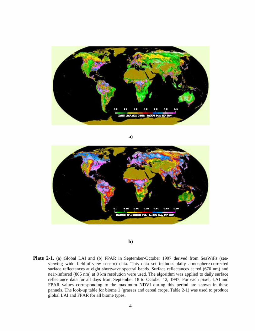
Table 2-1. Canopy Structural Attributes of Global Land Covers From the Viewpoint of RadiativeTransfer Modeling

Grasses and

Cereal Crops Shrubs BroadleafCrops

Savannas Broadleaf Forests Needle Forests

Horizontal heterogeneity no yes variable yes yes yes

Ground cover 100% 20-60% 10-100% 20-40% > 70% > 70%

Vertical heterogeneity

(leaf optics and LAD) no no no yes yes yes

Stems/trunks no no green stems yes yes yes

Understory no no no grasses yes yes

Foliage dispersion minimalclumping

random regular minimalclumping

clumped severeclumping

Crown shadowing no not mutual no no yes mutual yes mutual

Brightness of canopy

ground medium bright dark medium dark dark

The canopy structure is the most important variable determining the three-dimensionalradiation field in vegetation canopies. Therefore section 2.3 starts with a precise mathematicaldefinition of this variable and how various canopy radiation models treat this variable. Thisallows us to specify some common properties of the present canopy radiation models. The basicphysical principle underlying the proposed LAI/FPAR retrieval algorithm is the law of energyconservation. However, a rather wide family of canopy radiation models (described in theAppendix) conflict with this law. Therefore the three-dimensional transport equation whichincludes a nonphysical internal source is taken as the starting point for the derivation of thealgorithm. In section 2.5, a technique developed in atmospheric optics is utilized to parameterizethe radiative field in terms of reflectance properties of the canopy and ground, as well as to splitthe radiative transfer problem into two independent sub-problems, each of which is expressed interms of three basic components of the energy conservation law: canopy transmittance,reflectance, and absorptance. These components are elements of the look-up table (LUT), and thealgorithm interacts only with the elements of the LUT. This provides the required independenceof the retrieval algorithm to a particular canopy radiation model. The next important step inachieving property (3) is to specify the dependence of canopy transmittance, reflectance, andabsorptance on wavelength. It is precisely derived in section 2.6; this dependence is described bya simple function which depends on the unique positive eigenvalue of the transport equation. Theeigenvalue relates optical properties of individual leaves to canopy structure. This result not onlyallows a significant reduction in the size of the LUT but also relates canopy spectral reflectancewith spectral properties of individual leaves, which is a rather stable characteristic of greenleaves.

6

In spite of the essential reduction of possible canopy representatives by introducing avegetation cover classification, the inverse problem still allows for multiple solutions. Atechnique allowing the reduction of nonphysical solutions is described in section 2.7. Adefinition of the LUT is given in this section as well. A method to estimate the most probableLAI and FPAR, accounting for specific features of the MODIS and MISR instruments, andproviding convergence of the algorithm is discussed in sections 2.8 and 2.10. The maximumpositive eigenvalue and the unique positive eigenvector corresponding to this eigenvalue,detailed in section 2.6, express the law of energy conservation in a compact form. The results ofthis section allow us to relate the Normalized Difference Vegetation Index (NDVI) to thisfundamental physical principle. Relationships between FPAR and NDVI are also used in ouralgorithm as a backup to the LUT approach, and so we discuss these in section 2.11.

2.2 Canopy Structural Types of Global Vegetation

Solar radiation scattered from a vegetation canopy and measured by satellite sensors resultsfrom interaction of photons traversing through the foliage medium, bounded at the bottom by aradiatively participating surface. Therefore to estimate the canopy radiation regime, threeimportant features must be carefully formulated [Ross, 1981]. They are (1) the architecture ofindividual plants or trees and the entire canopy; (2) optical properties of vegetation elements(leaves, stems) and ground; the former depends on physiological conditions (water status,pigment concentration); and (3) atmospheric conditions which determine the incident radiationfield. Photon transport theory aims at deriving the solar radiation regime, both within thevegetation canopy and radiant exitance, using the above mentioned attributes as input data. Thisunderlies a land cover classification [Myneni et al., 1997] which is compatible with the basicphysical principle of transport theory, the law of energy conservation. Global land covers can beclassified into six types (biomes), depending on their canopy structure (Table 2-1). The structuralattributes of these land covers can be parameterized in terms of variables that transport theoryadmits as follows.

The heterogeneity of the plant canopy can be described by the three-dimensional leaf areadistribution function uL. Its values at spatial points depend on trunk distribution, topography,stem-trunk-branch area fraction, foliage dispersion, leaf and crown size, and leaf clumping[Myneni and Asrar, 1991; Oker-Blom et al., 1991]. The three-dimensional distribution of leavesdetermines various models to account for shadowing effects [Kuusk, 1985; Li and Strahler,1985; Verstraete et al., 1990]. The leaf area index LAI is defined as

∫⋅=

V

drruYX

)(1

LAI LSS

, (1)

where V is the domain in which a plant canopy is located; XS, YS are horizontal dimensions of V.If the vegetation canopy consists of Nc individual trees, LAI can be expressed as

∑∫∑==

⋅==CC

1L

1

LAI)(1

LAIN

kkk

V

N

k kk pdrru

Sp

k

,

7

where Sk is the foliage envelope projection (e.g., crown) of the kth plant or tree onto the ground;pk=Sk/(XS⋅YS) and LAIk is the leaf area index of an individual plant or tree. Thus LAI is

LAI = g⋅LAI 0 ,

where ∑=

=C

1

N

kkpg is the ground cover and

∑=

⋅=C

10 LAI

1LAI

N

kkkp

gis the mean LAI of a single plant or tree. The spatial distribution of plants or trees in the stand isa characteristic of the biome type and is assumed known. For each biome type, the leaf areadensity distribution function is parameterized in terms of ground cover and mean leaf area indexof an individual plant or tree, each varying within given biome specific intervals [gmin, gmax] and[Lmin, Lmax], respectively. Thus the vegetation canopy is represented as a domain V consisting ofidentical plants or trees in order to numerically evaluate the transport equation.

To parameterize the contribution of the surface underneath the canopy (soil and/orunderstory) to the canopy radiation regime, an effective ground reflectance is introduced,namely,

∫∫∫

−

Ω′ΩΩ′′Ω′

Ω′ΩΩΩ′′⋅ΩΩ′= +−

πλ

πλλ

π

µ

µµ

πλρ

2

0b

2

0b,b

2eff,

),,()(

),,(),(1

)(drLq

ddrLR

q . (2)

Here Lλ is radiance at a point rb of the canopy bottom; Rb,λ is the bidirectional reflectancefactor of the canopy bottom. The function q is a wavelength-independent configurable functionused to better account for specific features of various biomes, and it satisfies the followingcondition:

q d( )′ ′ =−

∫ Ω Ω 12π

. (3)

Note that the effective ground reflectance depends on the radiation regime in thevegetation canopy. It follows from the definition that the variation of ρq,eff satisfies the followinginequality:

)(

),(1

max),()(

),(1

min 2

,b

2beff,

2

,b

2 Ω′

ΩΩΩ′≤≤

Ω′

ΩΩΩ′ ∫∫+

−∈Ω′

+

−∈Ω′ q

dR

rq

dR

qπ

λ

π

πλ

π

µ

πλρ

µ

π ; (4)

that is, the range of variations depends on the integrated bidirectional factor of the groundsurface only. The bidirectional reflectance factor of the ground surface Rb,λ and the effectiveground reflectance are assumed to be horizontally homogeneous; that is, they do not depend onthe spatial point rb. The pattern of the effective ground reflectances (ρ1, ρ2, …, ρ11), ρi=ρq,eff(λi),at the MODIS spectral bands, is taken as a parameter characterizing hemispherically integratedreflectance of the canopy ground (soil and/or understory) and can vary continuously within the

8

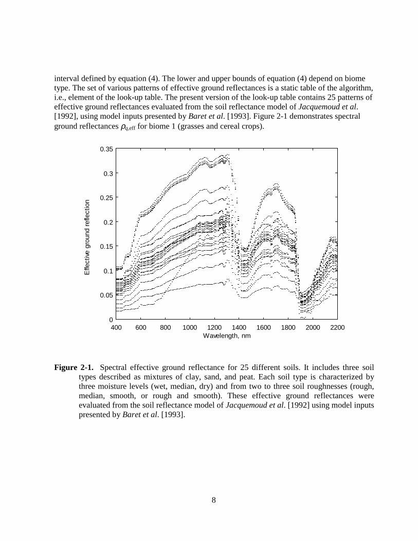
interval defined by equation (4). The lower and upper bounds of equation (4) depend on biometype. The set of various patterns of effective ground reflectances is a static table of the algorithm,i.e., element of the look-up table. The present version of the look-up table contains 25 patterns ofeffective ground reflectances evaluated from the soil reflectance model of Jacquemoud et al.[1992], using model inputs presented by Baret et al. [1993]. Figure 2-1 demonstrates spectralground reflectances ρq,eff for biome 1 (grasses and cereal crops).

0

0.05

0.1

0.15

0.2

0.25

0.3

0.35

400 600 800 1000 1200 1400 1600 1800 2000 2200

Effe

ctiv

e gr

ound

ref

lect

ion

Wavelength, nm

Figure 2-1. Spectral effective ground reflectance for 25 different soils. It includes three soiltypes described as mixtures of clay, sand, and peat. Each soil type is characterized bythree moisture levels (wet, median, dry) and from two to three soil roughnesses (rough,median, smooth, or rough and smooth). These effective ground reflectances wereevaluated from the soil reflectance model of Jacquemoud et al. [1992] using model inputspresented by Baret et al. [1993].

9

To account for the anisotropy of the ground surface, an effective ground anisotropy Sq isused,

0n,,),()(

),(),(1

)(

1),( bbb

2

b

2

b,b

,b <•Ω∈

Ω′Ω′′Ω′

Ω′Ω′′ΩΩ′⋅=Ω

∫∫

−

−Vr

drLq

drLR

rSeffq

q δµ

µ

πλρπ

λ

πλλ

, (5)

where nb is the outward normal at point rb. The effective ground anisotropy Sq depends on thecanopy structure as well as the incoming radiation field. We note the following property:

S r dq b( , )Ω Ωµπ

=+

∫ 12

,

that is, the integral depends neither on spatial nor on spectral variables. For each biome type, theeffective ground anisotropy is assumed wavelength independent. The six cover types presentedin Table 2-1 can now be expressed in terms of the above introduced variables.

2.2.1 Biome 1: Grasses and Cereal Crops

Canopies exhibit vertical and lateral homogeneity, vegetation ground cover of about 1.0(gmin=gmax=1), plant height generally about a meter or less, erect leaf inclination, no woodymaterial, minimal leaf clumping, and soils of intermediate brightness. The one-dimensionalradiative transfer model is invoked in this situation. Leaf clumping is implemented by modifyingthe projection areas with a clumping factor generally less than 1. The soil reflection is assumedLambertian; that is, Rb,λ=Rlam,λ. We also set q=1. The effective soil reflection and anisotropy thenhave the simplified form

ρq,eff(λ)=Rlam,λ , Sq(rb,Ω)=1/π . (6)

2.2.2 Biome 2: Shrubs

Canopies exhibit lateral heterogeneity, low (gmin=0.2) to intermediate (gmin=0.6) vegetationground cover, small leaves, woody material, and bright backgrounds. The full three-dimensional(3-D) model is invoked. Hot spot, i.e., enhanced brightness about the retrosolar direction due toabsence of shadows [Privette et al., 1994], is modeled by shadows cast on the ground (no mutualshadowing because ground cover is low). This land cover is typical of semiarid regions withextreme hot (brush) or cold (tundra/taiga) temperature regimes and poor soils. For this biome werepresent the bidirectional soil reflectance factor Rb,λ as

),()(),( 0,2,1,b ΩΩ⋅Ω′=ΩΩ′ λλλ RRR , (7)

where Ω0 is the direction of the direct solar radiance. We set*,1,1 )()( λλ ρΩ′=Ω′ Rq . (8)

10

The effective soil reflection and soil anisotropy then have the form

)()( 0*,2

*,1eff, Ω⋅= λλ ρρλρq ,

)(

),(1)(

0*,2

0,2

ΩΩΩ

⋅=Ωλ

λ

ρπR

Sq , (9)

where

∫−

Ω′′Ω′=π

λλ µπ

ρ2

,1*,1 )(

1dR , ∫

+

ΩΩΩ=Ωπ

λλ µπ

ρ2

0,20*,2 ),(

1)( dR .

The functions q and Sq are assumed wavelength independent and serve as parameter of thisbiome. This biome is characterized by intermediate vegetation ground cover. The use of theabove model for the bidirectional soil reflectance factor means that only the incoming directbeam of solar radiation which reaches the soil can influence the anisotropy of the radiation fieldin the plant canopy.

2.2.3 Biome 3: Broadleaf Crops

Canopies exhibit lateral heterogeneity, large variations in vegetation ground cover fromcrop planting to maturity (gmin=0.1, gmax=1.0), regular leaf spatial dispersion, photosyntheticallyactive, i.e., green, stems, and dark soil backgrounds. The regular dispersion of leaves (i.e., thepositive binomial model) leads to a clumping factor that is generally greater than unity. Thegreen stems are modeled as erect reflecting protrusions with zero transmittance. The three-dimensional radiative transfer model is invoked in this situation. The soil reflection is assumedLambertian, i.e., Rb,λ=Rlam,λ. ,λ. The function q=1. The effective soil reflection and anisotropy areexpressed by equation (6).

2.2.4 Biome 4: Savanna

Canopies with two distinct vertical layers, understory of grass, low ground cover ofoverstory trees (gmin=0.2, gmax=0.4), canopy optics, and structure are therefore verticallyheterogeneous. The full 3-D method is required. The interaction coefficients have a strongvertical dependency. Savannas in the tropical and subtropical regions are characterized asmixtures of warm grasses and broadleaf trees. In the cooler regimes of the higher latitudes, theyare described as mixtures of cool grass and needle trees. The effective soil reflection and soilanisotropy then are simulated by equation (9).

2.2.5 Biome 5: Broadleaf Forests

Vertical and lateral heterogeneity, high ground cover (gmin=0.8, gmax=1.0), greenunderstory, mutual shadowing of crowns, foliage clumping, trunks, and branches are included, sothe canopy structure and optical properties differ spatially. Mutual shadowing of crowns ishandled by modifying the hot spot formulation. Therefore stand density and crown size definethis gap parameter. The branches are randomly oriented, but tree trunks are modeled as erectstructures. Both trunk and branch reflectance are specified from measurements. For this biomethe three-dimensional transport equation is utilized to evaluate the effective soil reflection and

11

anisotropy as a function of LAI and Sun position. These are intermediate calculations and areused to precompute parameters stored in the LUT.

2.2.6 Biome 6: Needle Forests

These are canopies with needles, needle clumping on shoots, severe shoot clumping inwhorls, dark vertical trunks, sparse green understory, and crown mutual shadowing. This is themost complex case, invoking the full 3-D method with all its options. A typical shoot is modeledto handle needle clumping on the shoots. The shoots are then assumed to be clumped in thecrown space. Mutual shadowing by crowns is handled by modifying the hot spot formulation.The branches are randomly oriented but the dark tree trunks are modeled as erect structures. Bothtrunk and branch reflectance are specified from measurements. The effective soil reflection andanisotropy are evaluated the same way as for biome 5.

2.3 Radiative Transfer Problem for Vegetation Media

The domain V in which a vegetation canopy is located, is a parallelepiped of horizontaldimensions XS, YS, and biome-dependent height ZS. The top δVt, bottom δVb, and lateral δVl

surfaces of the parallelepiped form the canopy boundary δV=δVt+δVb+δVl. The structure of thevegetation canopy is defined by an indicator function χ(r) whose value is 1, if there is aphytoelement at the spatial point r, and zero otherwise. Here the position vector r denotes theCartesian triplet (x,y,z) with (0<x<XS), (0<y<YS), and (0<z<ZS), with its origin O=(0,0,0) at thetop of the canopy. The indicator function is treated as a random variable. Its distributionfunction, in the general case, depends on both macroscale (e.g., random dimension of the treesand their spatial distribution) and microscale (e.g., structural organization of an individual tree)properties of the vegetation canopy and includes all three of its components, absolutelycontinuous, discrete, and singular [Knyazikhin et al., 1998c]. In order to approximate thisfunction, a fine spatial mesh is introduced by dividing the domain V into Nε nonoverlapping finecells, ei, i= 1,2, … , Nε, of size ∆x=∆y=∆z. Each realization χ(r) of the canopy structure isreplaced by its mean over the fine cell ei as

i

ei

erdrmrem

rui

∈= ∫ ,)()()(

1)(L χ . (10)

Here m is a measure suitable to perform the integration of equation (10). The function uL isthe leaf area density distribution function. In the general case, (10) is the Lebesgue integral and itmay not coincide with an integral in the “true sense.” This integration technique provides theconvergence process uL→χ/m(V) when ε→0 [Knyazikhin et al., 1998c], and so equation (10) canbe taken as an approximation of the structure of the vegetation canopy. The accuracy of thisapproximation depends on size ε of the fine cell ei. To our knowledge, all existing canopyradiation models are based on the approximation of (10) by a piece-wise continuous function,e.g., describing both the spatial distribution of various geometrical objects like cones, ellipsoids,etc., and the variation of leaf area within a geometrical figure [Ross and Nilson, 1968; Nilson,1977; Ross 1981; Norman and Wells, 1983; Li et al., 1995]. Therefore we proceed with thesuggestion that uL is the random value whose distribution function is described by a piece-wise

12

continuous function. For each realization, the radiation field in such a medium can be expressedas

Ω′Ω′Ω→Ω′Γ=ΩΩ+Ω∇•Ω ∫ drLrru

rLrurGrL ),(),()(

),()(),(),(4

LL

πλλλλ π

. (11)

Here Ω•∇ is the derivative at r along the direction Ω; Lλ is the monochromatic radiance atpoint r and in the direction Ω,

L

2

LLL ),(2

1),( ΩΩ•ΩΩ=Ω ∫

+

drgrGππ

,

is the mean projection of leaf normals at r onto a plane perpendicular to the direction Ω; gL is theprobability density of leaf normal distribution over the upper hemisphere 2π+;

∫+

ΩΩ→Ω′ΩΩ•Ω′Ω=Ω→Ω′Γπ

λλ γππ

2

LL,LLLL ),,(),(2

1),(

1drrgr ,

is the area-scattering phase function [Ross, 1981], and γL,λ is the leaf-scattering phase function.Unit vectors are expressed in spherical coordinates with respect to (−Z) axis. It follows from theabove definitions that the solution of the transport equation is also a random variable. For eachbiome type, the angular distribution of radiance leaving the top surface of the vegetation canopyis defined to be the mean value, <Lλ>bio, of Lλ over different realizations of the given biome type.The following definitions of biome-specific reflectances are used in this paper.

The hemispherical-directional reflectance factor (HDRF) for nonisotropic incidentradiation is the ratio of the mean radiance leaving the top of the plant canopy, <Lλ(r t,Ω)>bio,Ω•nt>0, to radiance reflected from an ideal Lambertian target into the same beam geometry andilluminated under identical atmospheric conditions [Diner et al., 1998a]; that is,

0n,n),,(

1),(

),( t

2

t0t

biot0 >•Ω

Ω′•Ω′ΩΩ′

>Ω<=ΩΩ

∫−π

λ

λλ

πdrL

rLr .

Here nt is the outward normal at points r t∈δVt; <⋅>bio denotes the averaging over theensemble of biome realizations; and Ω0 is the direction of the monodirectional solar radiationincident on the top of the canopy boundary.

The bihemispherical reflectance (BHR) for nonisotropic incident radiation is the ratio ofthe mean radiant exitance to the incident radiant [Diner et al., 1998a], i.e.,

∫∫

−

+

Ω′•Ω′ΩΩ′

Ω•Ω>Ω<=Ω

πλ

πλ

λ

2

t0t

2

tbiot

0hem

n),,(

n),(

)(drL

drL

A .

In order to quantify a proportion between direct and diffuse component of incomingradiation, the ratio fdir(Ω0) of direct radiant incident on the top of the plant canopy to the total

13

incident irradiance is used. If fdir=1, HDRF and BHR become the bidirectional reflectance factor(BRF), and the directional hemispherical reflectance (DHR). Here rλ(Ω,Ω0) and )( 0

hem ΩλA

denote, depending on the situation (fdir=1 or fdir≠1), HDRF and BHR or BRF and DHR.

In spite of the diversity of canopy reflectance models, they can be classified with respect tohow the averaging over the ensemble of canopy realizations is performed. In terms of equation(11), this is equivalent to how the averaging of uL(r)Lλ(r,Ω) is performed. In the turbid mediummodels, the vegetation canopy is treated as a gas with nondimensional planar scattering centers[Ross, 1981]. Such models presuppose that

biobioLbioL ),()(),()( Ω=Ω rLrurLru λλ . (12)

As a result, equation (10) is reduced to the classical transport equation [Ross, 1981] whosesolution is the mean radiance < Lλ(r,Ω)>bio. This technique allows the design of conservativeradiation transfer models, i.e., models in which the law of energy conservation holds true for anyelementary volume. Such an approach cannot account for the hot spot phenomena because itignores shadowing effects. This motivated the development of a family of radiative transfermodels based on the following fact: the two events that a point inside a leaf canopy can beviewed from two points r1 and r2 are not independent [Kuusk, 1985]. The mean of uL(r)Lλ(r,Ω) ispresented as

bioLbioL ),()(),,(),()( Ω⋅Ω′Ω=Ω rLrurprLrubio λλ ,

where p is the bidirectional gap probability [Kuusk, 1985; Li and Strahler, 1985; Verstraete etal., 1990; Oker-Blom et al., 1991]. Such models account accurately for once scattered radiance,taking Gp<uL> as the extinction coefficient. For evaluation of the multiply scattered radiance,assumption (12) is usually used [Marshak, 1989; Myneni et al., 1995b]. These types of canopy-radiation models can well simulate BRFs. However, they are not conservative (Appendix 1). Theproblem of obtaining a correct closed equation for the mean monochromatic radiance wasformulated and solved by Vainikko [1973], where the equations for the mean radiance werederived through spatial averaging of the stochastic transport equation (11) in a model of brokenclouds. This approach was studied in detail by Titov [1990]. Anisimov and Menzulin [1981]utilized similar ideas to describe the radiation regime in plant canopies. The stochastic modelsincorporate the best features of the above mentioned approaches. The aim of this paper is toderive some general properties of radiation transfer which do not depend on a particular modeland which can be taken as the basis of our LAI/FPAR retrieval algorithm. Equation (11) expressthe law of energy conservation in the most general form. Therefore our aim can be achieved, ifthis equation is taken as a starting point for deriving the desired properties. In order to includecanopy reflectance models with hot spot effect into consideration, a transport equation of theform

),(),(),()(

),()(),(),(4

LL Ω+Ω′Ω′Ω→Ω′Γ=ΩΩ+Ω∇•Ω ∫ rFdrLr

rurLrurGrL λ

πλλλλ π

(13)

will also be considered in this paper. Here Fλ is a function which accounts for the hot spot effect.

14

Equation (13) alone does not provide a full description of random realizations of theradiative field. It is necessary to specify the incident radiance at the canopy boundary δV i.e.,specification of the boundary conditions. Because the canopy is adjacent to the atmosphere, andneighboring canopies, and the soil or understory, all which have different reflection properties,the following boundary conditions will be used to describe the incoming radiation [Ross et al.,1992]:

0n,),()(),,(),( ttt0ttop

0ttop

,dt ,m<•Ω∈Ω−Ω+ΩΩ=Ω VrrLrLrL δδ

λλλ , (14)

,0n,,)()(),(

n),(),(1

),(

lll0llat

,mllat

,d

0n

ll,ll

l

<•Ω∈Ω−Ω+Ω+

Ω′•Ω′Ω′ΩΩ′=Ω ∫>•Ω′

VrrLrL

drLRrL

δδ

π

λλ

λλλ

(15)

0n,,n),(),(1

),(0n

bbbbb,bb

b

<•Ω∈Ω′•Ω′Ω′ΩΩ′=Ω ∫>•Ω′

VrdrLRrL δπ λλλ , (16)

where top,d λL and top

,m λL are the diffuse and monodirectional components of solar radiation incident

on the top surface of the canopy boundary δVt; Ω0∼(µ0,φ0) is the direction of the monodirectionalsolar component; δ is the Dirac delta function; lat

,m λL is the intensity of the monodirectional solar

radiation arriving at a point r l∈δVl along Ω0 without experiencing an interaction with theneighboring canopies; )( l

lat,d rL λ is the diffuse radiation penetrating through the lateral surface δVl;

Rl,λ and Rb,λ (in sr-1) are the bidirectional reflectance factors of the lateral and the bottomsurfaces, respectively; and nt, nl, and nb are the outward normals at points r t∈δVt, r l∈δVl andrb∈δVb, respectively. A solution of the boundary value problem, expressed by equations (13)-(16), describes a random realization of the radiation field in a vegetation canopy.

2.4 Assumptions in Radiation Transfer Process

Theoretically, the sets DA and Dr can be generated offline by solving the transport equationat four MISR spectral bands for various combination of Sun-sensor geometry and all canopyrealizations from the set P. However, one can realize it only if the sets DA and Dr can bereprocessed with minimum effort. The time required to precompute these sets is a direct functionof the number of spectral channels used, combinations of Sun-sensor geometry, and elements inthe set P. For example, the generation of the set Dr using this direct method takes approximately192 computer hours of medium performance IBM RS/6000 RISC workstation [Running et al.,1996]. The size of Dr containing BRFs for two spectral bands and for all six biomes is about 63megabites. The inclusion of more spectral bands and view directions leads to significantdemands on the core memory required to execute this algorithm. It makes this approachimpractical in the case of MISR instrument. The aim of this section and section 2.5 is toformulate some assumptions allowing for a significant reduction in the size of DA and Dr.

15

2.4.1 Conservativity

A radiative transfer model is defined to be conservative if the law of energy conservationholds true for any elementary volume [Bass et al., 1986]. Within a conservative model, radiationabsorbed, transmitted, and reflected by the canopy is always equal to radiation incident on thecanopy. A rather wide family of canopy radiation models [Kuusk, 1985; Marshak, 1989; Pinty etal., 1989; Li and Strahler, 1992; Myneni et al., 1995; Pinty and Verstraete, 1998] which accountfor the hot spot are equivalent to the solution of the above boundary value problem in which thefunction Fλ has the following form [Knyazikhin et al., 1998a]:

Fλ(r,Ω) = [σ(r,Ω) - σH(r,Ω,Ω0)]LH,λ(r,Ω).

Here LH,λ is the upwardly directed once-scattered radiance produced by the hot spot, andσH is a model-dependent total interaction cross section, introduced in canopy radiation models toaccount for the hot spot effect and to evaluate LH,λ. The total interaction cross section σ is used toevaluate the attenuation of both direct solar radiance and multiply scattered radiance. Because Fλcan take on negative values, it has no physical meaning in terms of energy conservation. Thesetypes of canopy radiation models are mainly used to fit simulated BRFs to measured BRFs.However, the ability of a model to simulate canopy reflection is not a sufficient requisite for thesolution of the inverse problem. Canopy radiation models must also satisfy the law of energyconservation and provide the correct proportions of canopy absorptance, transmittance, andreflectance. Because the retrieval algorithm is based on energy conservation, the following“minimum” requirement, which the canopy radiation models must satisfy in order to be usefulfor inverse problems, is formulated:

dr d F rV∫ ∫ =Ω Ωλ

π

( , ) ,4

0

for any λ. This equation does not allow a nonphysical source Fλ(r,Ω) to influence thecanopy radiative energy balance. Currently, we use a model for σH proposed by Myneni et al.[1995]. A nonconservative canopy radiation model must be corrected, as described in section2.7.

2.4.2 Leaf Area Index

The leaf area index LAI is defined as

∫=V

drruYX

)(1

LAI LSS

.

If the vegetation canopy consists of Nc individual trees, LAI can be expressed as

∑∫∑==

==cc

1L

1

LAI)(1

LAIN

kkk

V

N

k kk gdrru

Sg

k

,

16

where Sk is the crown projection of the kth tree onto the ground; gk=Sk/(XSYS) and LAIk is the leaf

area index of an individual tree. Thus LAI is LAI = gLAI 0, where ∑ == c

1

N

k kgg is the ground

cover, and

∑=

⋅=c

10 LAI

1LAI

N

kkkg

gis the mean LAI of a single tree. The spatial distribution of trees in the stand is a characteristic ofthe biome type and is assumed to be random. For each biome type, the leaf area densitydistribution function is parameterized in terms of the ground cover and mean leaf area index ofan individual tree, each varying within given biome-specific intervals [gmin, gmax] and [Lmin,Lmax], respectively. Thus the vegetation canopy is represented as a domain V consisting ofidentical trees in order to numerically evaluate the transport equation.

2.4.3 Anisotropy of Incoming Diffuse Radiation

A model of clear-sky radiance proposed by Pokrowski [1929] is used to approximate theratio between the angular distribution of incoming diffuse radiation and its flux:

0,),(~,1

132.0exp1

),(

),(

0

0

2

ttop

,d

ttop

,d <ΩΩ•Ω−Ω•Ω+

−−=ΩΩ

Ω

∫−

µφµµµ

πλ

λ

drL

rL.

We assume that this ratio does not depend on wavelength. The diffuse radiation top,d λL does

not depend on the top boundary space point r t∈δVt. This allows the parameterization of theincoming radiation field in terms of fdir and the total (diffuse and direct) incident flux.

2.4.4 Boundary Conditions for Lateral Surface

The radiation penetrating through the lateral sides of the canopy depends on theneighboring environment. Its influence on the radiation field within the canopy is especiallypronounced near the lateral canopy boundary. Therefore inaccuracies in the lateral boundaryconditions may cause distortions in the simulated radiation field within the domain V. Thesedistortions, however, decrease with distance from this boundary toward the center of the domain.The size of the “distorted area“ depends on the adjoining vegetation, atmospheric conditions, andmodel resolution [Kranigk, 1996]. In particular, it has been shown that these lateral effects canbe neglected when the radiation regime is analyzed in a rather extended canopy, as is the caseconsidering the rather large MISR pixel (~1.1 km). Therefore we idealize our canopy as ahorizontally infinite region. We will use a “vacuum” boundary condition for the lateral surface tonumerically evaluate a solution for the case of a horizontally infinite domain,

Lλ(r l,Ω) = 0, r l∈δVl, Ω • nl < 0.

17

2.4.5 Optical Properties of Foliage

The leaf-scattering phase function γL,λ is assumed to be bi-Lambertian [Ross and Nilson,1968]; that is, a fraction of the energy intercepted by the foliage element is reflected ortransmitted in a cosine distribution about the leaf normal,

>Ω•Ω′Ω•ΩΩ•Ω

<Ω•Ω′Ω•ΩΩ•Ω=Ω→Ω′Ω

−

−

.0))((,)(

,0))((,)(),,(

LLL,D1

LLL,D1

L,Lrt

rrr

λ

λλ π

πγ

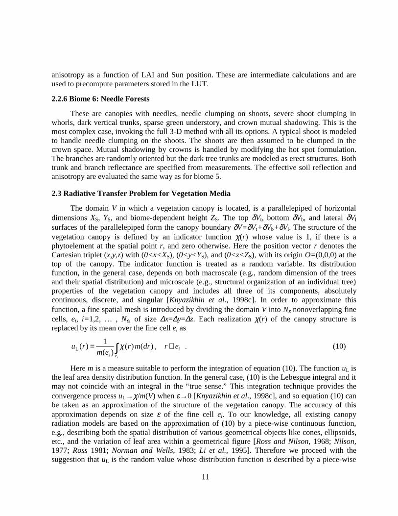
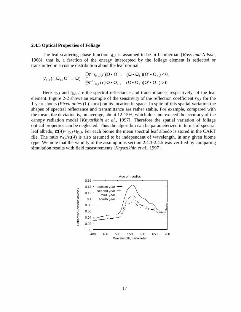
Here rD,λ and tD,λ are the spectral reflectance and transmittance, respectively, of the leafelement. Figure 2-2 shows an example of the sensitivity of the reflection coefficient rD,λ for the1-year shoots (Picea abies (L) karst) on its location in space. In spite of this spatial variation theshapes of spectral reflectance and transmittance are rather stable. For example, compared withthe mean, the deviation is, on average, about 12-15%, which does not exceed the accuracy of thecanopy radiation model [Knyazikhin et al., 1997]. Therefore the spatial variation of foliageoptical properties can be neglected. Thus the algorithm can be parameterized in terms of spectralleaf albedo, ω(λ)=rD,λ+tD,λ. For each biome the mean spectral leaf albedo is stored in the CARTfile. The ratio rD,λ/ω(λ) is also assumed to be independent of wavelength, in any given biometype. We note that the validity of the assumptions section 2.4.3-2.4.5 was verified by comparingsimulation results with field measurements [Knyazikhin et al., 1997].

0

0.02

0.04

0.06

0.08

0.1

0.12

0.14

0.16

400 450 500 550 600 650 700

Ref

lect

ion

(dim

ensi

onle

ss)

Wavelength, nanometer

Age of needles

current yearsecond year

third yearfourth year

18

0

0.02

0.04

0.06

0.08

0.1

0.12

0.14

0.16

400 450 500 550 600 650 700

Ref

lect

ion

(dim

ensi

onle

ss)

Wavelength, nanometer

Position of the tw ig

upperupper middlelow er middle

low er

0

0.02

0.04

0.06

0.08

0.1

0.12

0.14

0.16

400 450 500 550 600 650 700

Ref

lect

ion

(dim

ensi

onle

ss)

Wavelength, nanometer

Geographical orientation

southnortheast

south-east

Figure 2-2. Spectral reflectance of 1-year-old spruce shoots. Three characteristics of the 1-yearshoots were chosen to examine the spatial variations of foliage spectral properties, age ofneedles on the 1-year shoot; position within the tree crown (top, two middle, and bottom)and geographical orientation with respect to the tree stem (south, north, east and west).

2.4.6 Ground Reflectance and Anisotropy

To parameterize the contribution of the surface underneath the canopy (soil or/andunderstory) to the canopy radiation regime, an effective ground reflectance is introduced,namely,

0n,,),()(

),(),(

),( bbb

2

b

2

b,b

2beff, <•Ω∈

Ω′Ω′′Ω′

Ω′ΩΩ′′ΩΩ′=

∫∫∫

−

+− VrdrLq

ddrLR

rq δµπ

µµλρ

πλ

πλλ

π .

19

Here Lλ is the solution of the boundary value problem for the transport equation. Thefunction q is a configurable function used to better account for features of biomes [Knyazikhin etal., 1998a], and it satisfies the following condition:

q d( )′ ′ =−

∫ Ω Ω 12π

.

The effective ground reflectance depends on the canopy structure and the incident radiationfield. It follows from the definition that the variation of ρq,eff satisfies the following inequality:

)(

),(

max),()(

),(

min 2

,b

2beff,

2

,b

2 Ω′

ΩΩΩ′≤≤

Ω′

ΩΩΩ′ ∫∫+

−∈Ω′

+

−∈Ω′ q

dR

rq

dR

q π

µλρ

π

µπ

λ

π

πλ

π;

that is, the range of variation depends on the integrated bidirectional reflectance factor of theground surface only. For each biome type, the bidirectional reflectance factor of the groundsurface Rb,λ and the effective ground reflectance are assumed to be horizontally homogeneous;that is, they do not depend on the spatial point rb. Effective ground reflectances at the MISRspectral bands are elements of the canopy realization p∈P. Various patterns of the spectralground reflectance evaluated from the soil reflectance model of Jacquemoud et al. [1992] areincluded in the present version of the CART file.

To account for the anisotropy of the ground surface, we introduce an effective groundanisotropy Sq,

0n,,),()(

),(),(

)(

1),( bbb

2

b

2

b,b

eff,b <•Ω∈

Ω′Ω′′Ω′

Ω′Ω′′ΩΩ′=Ω

∫∫

−

− VrdrLq

drLR

rSq

q δµπ

µ

λρπ

λ

πλλ

.

The effective ground anisotropy Sq depends on the canopy structure as well as theincoming radiation field. We note the following property:

∫+

=ΩΩπ

µ2

b 1),( drSq ;

that is, the above integral depends neither on spatial nor on spectral variables. For each biometype, the effective ground anisotropy is assumed to be wavelength independent. The groundanisotropy is used to precompute some solutions of the transport equation and thus is not storedin the CART file.

2.5 Mathematical Basis of the Algorithm

The aim of this section is to parameterize the contribution of soil/understory reflectances tothe exitant radiation field. We closely follow ideas used in atmospheric physics [Kondratyev,1969; Liou, 1980]. It follows from the linearity of equation (13) that its solution can berepresented as the sum

Lλ(r,Ω) = Lbs,λ(r,Ω) + Lrest,λ(r,Ω) . (17)

20

Here Lbs,λ is the solution of the “black-soil problem” which satisfies equation (13) withboundary conditions expressed by equations (14), (15), and

Lbs,λ(rb,Ω) = 0, rb∈δVb, Ω•nb < 0 .

The function Lrest,λ also satisfies equation (13) with Fλ=0 and boundary conditionsexpressed as

Lrest,λ(r t,Ω) = 0, r t∈δVt, Ω•nt < 0 ,

0n,,n),(),(1

),( lll

0n

llrest,,llrest,

l

<•Ω∈Ω′•Ω′Ω′ΩΩ′=Ω ∫>•Ω′

VrdrLRrL δπ λλλ , (18)

0n,,n),(),(1

),(0n

bbbbb,bb,rest

b

<•Ω∈Ω′•Ω′Ω′ΩΩ′=Ω ∫>•Ω′

VrdrLRrL δπ λλλ . (19)

Note that Lrest,λ depends on the solution of the “complete transport problem.” The boundarycondition (19) can be rewritten as

Lrest,λ(rb,Ω) = ρq,eff(λ)Sq(rb,Ω)Tq,λ , (20)

where ρq,eff, and Sq are defined by (2) and (5), respectively, and

∫−

Ω′′Ω′Ω′=π

λλ µ2

bb, ),()()( drLqrTq . (21)

The function q is defined by (3). The coefficient ρq,eff is assumed to be independent of thepoint rb. It is taken as the parameter describing the reflectance of the surface underneath thecanopy and can vary continuously within a biome-dependent interval (section 2.3). The biome-dependent function Sq is assumed to be wavelength independent and known (section 2.3). Wereplace Tq,λ in (20) by its mean value over the ground surface. This implies that the variable Tq,λis independent on the space point rb (this is automatically fulfilled if a one-dimensional radiativetransfer model is used to evaluate the radiative field in plant canopies). Taking into accountequation (20), we then can rewrite the solution of the transport problem, equation (17), as

Lλ(r,Ω) = Lbs,λ(r,Ω) + ρq,eff(λ)⋅Tq,λLq,λ(r,Ω) , (22)where Lq,λ(r,Ω) satisfies equation (13) with Fλ=0, boundary condition expressed by equation(18), and

Lq,λ(r t,Ω) = 0, r t∈δVt, Ω•nt < 0 , (23)

Lq,λ(rb,Ω) = Sq(rb,Ω), rb∈δVb, Ω•nb < 0 . (24)

Thus Lq,λ(r,Ω) describes the radiation regime in a plant canopy generated by anisotropicand heterogeneous sources S(rb,Ω) located at the canopy bottom. We term the problem of findingLq,λ(r,Ω) an “S problem.” Substituting (22) in (21), we get

)()()()( b,,eff,,bsb, rTrTrT qqqbq

q λλλλ λρ r+= , (25)

where

21

∫−

Ω′′Ω′Ω′=π

λλ µ2

b,bsb,bs ),()()( drLqrT q ,

∫−

Ω′′Ω′Ω′=π

λλ µ2

b,b, ),()()( drLqr qqr .

We then average equation (25) over the ground surface. This allows us to express Tq,λ viaqT λ,bs , λ,qr , and ρq,eff. Substituting the averaged Tq,λ into equation (22), we get

),()(1

)(),(),( ,,bs

,eff,

eff,,bs Ω

−+Ω≈Ω rLTrLrL q

q

qq

qλλ

λλλ λρ

λρr

. (26)

Here qT λ,bs and λq,r are averages over the canopy bottom. Note that we can replace the

approximate equality in equation (26) by an exact equality if a one-dimensional canopy radiationmodel is used to evaluate the radiative regime. It follows from equation (26) that the BHR, hem

λA ,

HDRF, rλ, and the fraction of radiation absorbed by the vegetation, hemλa , at wavelength λ can be

expressed as

)()(1

)()()( 0

,hem,bs

,eff,

eff,,0

hem,bs0

hem Ω−

+Ω≈Ω q

qq

qqA λ

λλλλ λρ

λρt

rtr , (27)

)()(1

)()(),(),( 0

,hem,bs

,eff,

eff,,0,bs0 Ω

−⋅

Ω+ΩΩ≈ΩΩ q

qq

qqrr λ

λλλλ λρ

λρπτ t

r , (28)

)()(1

)()()( 0

,hem,bs

,eff,

eff,,0

hem,bs0

hem Ω−

+Ω≈Ω q

qq

qq λ

λλλλ λρ

λρt

raaa , (29)

where )( 0hem

,bs Ωλr , hem,bs λa , and rbs,λ are the BHR, HDRF, and the fraction of radiation absorbed by

the vegetation, respectively, when the canopy ground reflectance is zero. Here

∫−

Ω′Ω′′=Ω

πλ

λλ µ

2

t

,bs0

,hem,bs

),()(

drL

T qqt

is the weighted canopy transmittance,

∫+

Ω′Ω′′=π

λλ µ2

t,, ),( drLqqt

is the transmittance resulting from the anisotropic source Sq located at the canopy bottom, and

),()( t,, Ω=Ω rLqq λλτis the radiance generated by Sq which leaves the top of the plant canopy, and λ,qa is the radiance

generated by Sq and absorbed by the vegetation. The radiation reflected, transmitted, andabsorbed by the vegetation must be related via the energy conservation law,

22

)(

)()(,1)(

0,hem

,bs

01,hem

,bs0,

hem,bs

,hem,bs0,

hem,bs Ω

Ω=Ω=+⋅Ω+

≡

q

q

qq

q kkλ

λλλλλλ t

tatr , (30)

1,,, =++ λλλ qqq atr . (31)

Note that all the variables in equations (27) and (28) are mean values averaged over the topsurface of the canopy.

It follows from equation (27) that

)()(1

)()()( 0

,hem,bs

,ef,

eff,0

hem,bs0

hem Ω−

≈Ω−Ω q

qfq

qq,A λ

λλλλ λρ

λρt

rtr . (32)

Thus the contribution of the ground to the canopy-leaving radiance is proportional to thesquare of canopy transmittance and that the factor of proportionality depends on ρq,eff. If theright-hand side is sufficiently small, we can neglect this contribution by assigning a value of zeroto the effective soil reflectance.

Thus we have parameterized the solution of the transport problem in terms of ρq,eff andsolutions of the “black-soil problem” and “S problem.” The solution of the “black-soil problem”depends on Sun-view geometry, canopy architecture, and spectral properties of the leaves. The"S problem" depends on spectral properties of the leaves and canopy structure only. At this stage,these properties allow a significant reduction in the size of the LUT because there is no need tostore the dependence of the exiting radiation field on ground reflection properties. Since thesolution of the “black-soil problem” and “S problem” determine the size of the LUT, we focus onthe solution of these problems, using equation (26) as the basis of the algorithm. The next step isto specify the wavelength dependence of the basic algorithm equation.

2.6 Conservative Models

Let us consider equation (11) with boundary conditions expressed by equations (14)-(16).This boundary value problem can be reduced to the solution of the “black-soil problem” and “Sproblem.” In the LAI/FPAR retrieval algorithm the boundary conditions (15) for the lateralsurface of domain V are replaced by vacuum condition, i.e., Lλ(r l,Ω)=0 if r l∈δVl and Ω•nl<0[Diner et al., 1998b; Knyazikhin et al., 1998b]. The boundary condition of the “S problem”expressed by equations (18), (23), and (24) are wavelength independent in this case. Theincoming radiation (14) can be parameterized in terms of two scalar values: fdir,λ and total fluxF0,λ of incoming radiation. It allows representing the “black-soil problem” as a sum of tworadiation fields. The first is generated by the monodirectional component of solar radiationincident on the top surface of the canopy boundary and, the second, by the diffuse component.Dividing the transport equations and boundary conditions which define these problems byfdir,λ⋅F0,λ and (1-fdir,λ)F0,λ, one can reduce them to transport problems with wavelength-independent boundary conditions. Thus the spectral variation of the radiative field in vegetationcanopies can be described, when the spectral variation of the solution of the transport equation

23

with wavelength-independent boundary conditions is known. Therefore we consider thefollowing boundary value problem for the transport equation

Ω′Ω′Ω→Ω′=ΩΩ+Ω∇•Ω ∫ drrrrr ),(),(),(),(),(4

,s

πλλλλ ϕσϕσϕ , (33)

0n,,),(),( <Ω•∈Ω=Ω rVrrBr δϕλ . (34)

Here B is a wavelength-independent function defined on the canopy boundary δV, and nr isthe outward normal at the point r∈δV. Differentiating equations (33) and (34) with respect towavelength λ, we get

Ω′Ω′Ω→Ω′=ΩΩ+Ω∇•Ω ∫ drrd

drurru ),(),(),(),(),(

4

,s

πλλλλ ϕσ

λσ , (35)

0n,,0),( <Ω•∈=Ω rVrru δλ , (36)

where

λϕ

λ d

rdru

),(),(

Ω=Ω .

The following results from eigenvector theory are required to derive a relationship betweenspectral leaf albedo and canopy absorptance, transmittance, and reflectance.

An eigenvalue of the transport equation is a number γ such that there exists a function ϕwhich satisfies

[ ] ∫ Ω′Ω′Ω→Ω′=ΩΩ+Ω∇•Ωπ

λ ϕσϕσϕγ4

,s ),(),(),(),(),( drrrrr , (37)

with boundary conditions

ϕ(r,Ω)=0, r ∈ δV=δVt+δVb+δVl, nr•Ω < 0 .

The function ϕ(r,Ω) is termed an eigenvector corresponding to the given eigenvalue γ.

The set of eigenvalues γk, k=0,1,2, … and eigenvectors ϕk(r,Ω), k=0,1,2, … of the transportequation is a discrete set [Vladimirov, 1963]. The eigenvectors are mutually orthogonal; that is,

lklk

V

drdrrr ,

4

),(),(),( δϕϕσπ

=ΩΩΩΩ∫∫ (38)

where δk,l is the Kroneker symbol. The transport equation has a unique positive eigenvalue whichcorresponds to a unique positive (normalized in the sense of equation (38)) eigenvector[Germogenova, 1986]. This eigenvalue is greater than the absolute magnitudes of the remainingeigenvalues. This means that only one eigenvector, say ϕ0, takes on positive values for any r∈Vand Ω. This positive couplet of eigenvector and eigenvalue plays an important role in transporttheory, for instance, in neutron transport theory. This positive eigenvalue alone determines if thefissile assembly will function as a reactor, or as an explosive, or will melt. Its value successfullyrelates the reactor geometry to the absorption capacity of the active zone. Because the reactor is

24

controlled by changing the absorption capacity of the active zone (by inserting or removingabsorbents), this value is critical to its functioning. The similarity to the problem at hand is thatwe need to relate canopy architecture (“similar” to reactor geometry) with leaf optical properties(“similar” to the absorption capacity of the active zone). The expansion of the solution of thetransport equation in eigenvectors has mainly a theoretical value because the problem of findingthese vectors is much more complicated than finding the solution of the transport equation.However, this approach can be useful if we want to estimate some integrals of the solution.Therefore we apply this technique to derive a relationship between spectral leaf albedo andcanopy absorptance, transmittance, and reflectance.

Equation (35) with boundary conditions (36) is a linear homogeneous differential equationwith respect to λ in a functional space [Krein, 1972]. Its solution ϕ can be expanded ineigenvectors,

ϕ λ ϕ λ λ ϕ λλ ( , ) ( ) ( , , ) ( ) ( , , )r a r a rk kk

Ω Ω Ω= +=

∞

∑0 01

, (39)

where coefficients ak do not depend on spatial or angular variables. Here we separate the positiveeigenvector ϕ0 into the first summand. As described above, only this summand, a0ϕ0, takes onpositive values for any r∈V and Ω. Substituting (39) into equation (35), we get

[ ] ∫∑∑ Ω′Ω′Ω→Ω′=ΩΩ+Ω∇•Ω∞

=

∞

= πλ λϕσ

λλσλ

4

,00

),,(),(),,(),(),,( drard

drurru kks

kkkk , (40)

where uk=d(akϕk)/dλ. Substituting (37) into (40), further results in

[ ] [ ]∑∞

=

=

Ω−Ω−Ω+∇•Ω

0

0)(

),,()(),,()(1),(k

kkkkk d

drarur

λλγλϕλλλγσ .

Here γk(λ) is the eigenvalue corresponding to the eigenvector ϕk. It follows from thisequation, as well as from the orthogonality of eigenvectors, that

[ ] [ ]),,()()(1

)(),,()( Ω

−=Ω

rad

d

d

radkk

k

k

kk λϕλλγ

λλγ

λλϕλ

.

Solving this ordinary differential equation results in

[ ]),,()()(1

)(1),,()( 00

0 Ω−−=Ω rara kk

k

kkk λϕλ

λγλγλϕλ . (41)

Thus if we know the kth summand of the expansion in equation (39) at a wavelength λ0,we can easily find this summand for any other wavelength.

We introduce e, the monochromatic radiation at wavelength λ intercepted by thevegetation canopy,

∫∫ ΩΩΩ=π

λϕσλ4

),(),()( rrddrV

e , (42)

25

and e0 as

∫∫ ΩΩ⋅ΩΩ=π

λ λϕϕσλ4

00 ),,(),(),()( drdrrrV

e . (43)

Given e, we can evaluate the fraction a of radiation absorbed by the vegetation at thewavelength λ as

a(λ) = [1-ω(λ)]e(λ), (44)where

),(

),(1

)( 4

Ω′

ΩΩ→Ω′Γ=

∫rG

drπ

λ

πλω (45)

is the leaf albedo. Below an estimation of e0 will be performed. This value is close to e. We skipa precise mathematical proof of this fact here. An intuitive explanation is as follows: Putting (39)in (42) and integrating the series results in only the positive term containing a0ϕ0. As a result,e(λ)/e(λ0)≈e0(λ)/e0(λ0). Let us derive the dependence of e on wavelength. Substituting equation(39) into equation (43) and taking into account equation (41) as well as the orthogonality ofeigenvectors, equation (38), we obtain

)()(1

)(1)( 00

0

000 λ

λγλγλ ee

−−= ,

where γ0 is the positive eigenvalue corresponding to the positive eigenvector ϕ0. Taking intoaccount equation (44), we can also derive the following estimation for a:

)()(1

)(1

)(1

)(1)( 0

00

00 λλωλω

λγλγλ aa

−−⋅

−−= . (46)

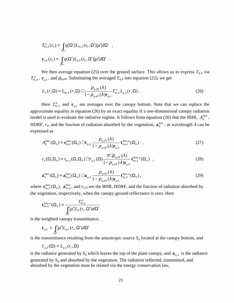
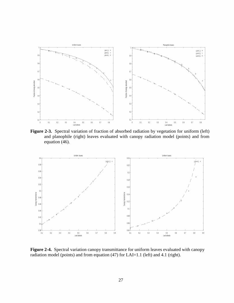
Thus given canopy absorptance at wavelength λ0, we can evaluate this variable at anyother wavelength. Figure 2-3 shows spectral variation of the fraction of energy absorbed by thevegetation canopy a for uniform and planophile leaves. Equation (46) can also be used to specifythe accuracy of a canopy radiation model to simulate the radiative field in the canopy. On can see(Figure 2-3, right) that our radiation model is erroneous in the case of planophile leaves whenLAI>5 and the leaf albedo ω>0.5. At a given wavelength, a is a function of canopy structure andSun position in the case of “black-soil problem,” and a function of canopy structure only in thecase of the “S problem.” We store a at a fixed wavelength λ0 in the LUT.

A somewhat more complicated technique is realized to derive an approximation for canopytransmittance,

−−=

)(

,)(1

)(1

)(, ,

00

00,

λωλ

λγλγ

λωλ λλ DD rr

tt , (47)

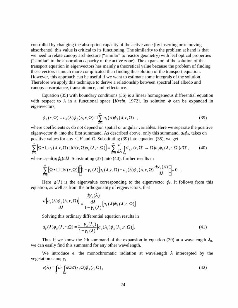
where rD,λ is the spectral reflectance of the leaf element. The ratio rD,λ/ω(λ) is assumed to beconstant with respect to wavelength for each biome. Thus given the canopy transmittance atwavelength λ0, we can evaluate this variable for wavelength λ. Figure 2-4 shows spectral

26

variation of canopy transmittance for uniform leaves evaluated with our canopy radiation modeland with equation (47). At a fixed wavelength, t is a function of canopy structure and Sunposition in the case of the “black-soil problem,” and a function of canopy structure in the case ofthe “S problem.” We store t at a fixed wavelength λ0 in the LUT.

The canopy reflectance r is related to the absorptance and transmittance via the energyconservation principle

r(λ) = 1 - t(λ) - a(λ) . (48)

Thus given canopy transmittance and absorptance at a fixed wavelength, we can obtain thecanopy reflectance for any wavelength. Figure 2-5 demonstrates an example of equation (48).

The unique positive eigenvalue γ0, corresponding to the unique positive eigenvector, canbe estimated as [Knyazikhin and Marshak, 1991]

γ0(λ) = ω(λ)[1 - exp(-K)] , (49)where K is a coefficient which may depend on canopy structure (i.e., biome type, LAI, groundcover, etc.) and Sun position but not on wavelength or soil type. Its specification depends on theparameter (absorptance or transmittance) and type of transport problem (“black-soil problem” or“S problem”). The coefficient K, however, does not depend on the transport problem and sunposition, when it refers to canopy absorptance. Figure 2-6 shows the coefficient K for the “Sproblem” and canopy absorptance as a function of LAI. This coefficient is an element of theLUT. Note that the eigenvalue γ0 depends on values of spectral leaf albedo (45) which, in turn,depends on wavelength. It allows us to parameterize canopy absorptance, transmittance, andreflectance in terms of canopy structure, Sun position and leaf albedo.

27

0 .1

0 .2

0 .3

0 .4

0 .5

0 .6

0 .7

0 .8

0 .9

1

0 0 .1 0 .2 0 .3 0 .4 0 .5 0 .6 0 .7 0 .8

Frac

tion o

f ene

rgy a

bsor

bed

L ea f a lbe do

U n ifo rm le a ve s

L AI=1.1L AI=5.1L AI=9.1

0 .1

0 .2

0 .3

0 .4

0 .5

0 .6

0 .7

0 .8

0 .9

1

0 0 .1 0 .2 0 .3 0 .4 0 .5 0 .6 0 .7 0 .8

Frac

tion o

f ene

rgy ab

sorbe

dL ea f a lb ed o

P la n op hile lea ves

L A I= 1 .1L A I= 5 .1L A I= 9 .1

Figure 2-3. Spectral variation of fraction of absorbed radiation by vegetation for uniform (left)and planophile (right) leaves evaluated with canopy radiation model (points) and fromequation (46).

0 .3 8

0 .4

0 .4 2

0 .4 4

0 .4 6

0 .4 8

0 .5

0 .5 2

0 .5 4

0 .5 6

0 .5 8

0 .6

0 .1 0 .2 0 .3 0 .4 0 .5 0 .6 0 .7 0 .8 0 .9

Cano

py tr

ansm

ittanc

e

L ea f a lb ed o

U n ifo rm lea ves

L A I= 1 .1

0 .0 4

0 .0 6

0 .0 8

0 .1

0 .1 2

0 .1 4

0 .1 6

0 .1 8

0 .2

0 .2 2

0 .2 4

0 .1 0 .2 0 .3 0 .4 0 .5 0 .6 0 .7 0 .8 0 .9

Cano

py tr

ansm

ittanc

e

L ea f a lb ed o

U n ifo rm lea ves

L A I= 4 .1

Figure 2-4. Spectral variation canopy transmittance for uniform leaves evaluated with canopyradiation model (points) and from equation (47) for LAI=1.1 (left) and 4.1 (right).

28

0

0 .0 5

0 .1

0 .1 5

0 .2

0 .2 5

0 .3

0 .3 5

0 .4

0 0 .1 0 .2 0 .3 0 .4 0 .5 0 .6 0 .7 0 .8

Direc

tiona

l hem

isphe

rical

reflec

tance

L ea f a lb ed o

U n ifo rm lea ves

L A I= 1 .1L A I= 4 .1

Figure 2-5. Spectral variation of the DHR for uniform leaves evaluated with canopy radiationmodel (points) and from equation (48) for LAI=1.1 and 4.1.

0

0 .2

0 .4

0 .6

0 .8

1

1 .2

1 .4

1 .6

1 .8

2

0 1 2 3 4 5 6 7 8 9 1 0

Coeff

icien

t K

L ea f a re a in de x

U n ifo rm lea ves

A b s o rbt ion

Figure 2-6. Coefficient K as a function of LAI for canopy absorptance.

29

2.7 Constraints on Look-Up Table Entries

In spite of the diversity of canopy reflectance models, their direct use in an inversionalgorithm is ineffective. In the case of forests, for example, the interaction of photons with therough and rather thin surface of tree crowns and with the ground in between the crowns are themost important factors causing the observed variation in the directional reflectance distribution.These phenomena are rarely captured by many canopy reflectance models. As a result, thesemodels are only slightly sensitive to the within-canopy radiation regime. This assertion is basedon the fact that a rather wide family of canopy radiation models are solutions to (13), includingmodels with a nonphysical internal source Fλ (Appendix). Within such a model the sum ofradiation absorbed, transmitted, and reflected by the canopy are not equal to the radiationincident on the canopy. The function Fλ is chosen such that the model simulates the reflectedradiation field correctly, i.e., these models account for photon interactions within a rather smalldomain of the vegetation canopy. On the other hand, it is the within-canopy radiation regime thatis very sensitive to the canopy structure and therefore to LAI. The within-canopy radiationregime also determines the amount of solar energy absorbed by the vegetation. Ignoring thisphenomenology in canopy radiation models leads to a large number of nonphysical solutionswhen one inverts a canopy reflectance model. Therefore (27) and (28) must be transformedbefore they can be used in a retrieval algorithm.

Let us introduce the required weights

1),(,)(

),(),(

2

0,bs0

hem,bs

0,bs1

0,bs =ΩΩΩΩ

ΩΩ=ΩΩ ∫

+

−

πλ

λ

λλ µ

πdw

rw

r , (50)

1)(,)(

)(2,

, =ΩΩΩ

=Ω ∫+π

λλ

λλ µ

τdww q

q

qq

t . (51)

With this notation, (28) can be rewritten as

)()(1

)()(),( 0

,hem,bs

,eff,

eff,,0

hem,bs,bs0 Ω

−+Ω⋅≈ΩΩ q

qq

qq

qwwr λλ

λλλλλ λρλρ

ππ tr

tr (52)

and from (30) and (31), the canopy reflectances hem,bs λr and λ,qr can be written as

hem,bs

1,hem,bs

hem,bs 1 λλλ atr −−= ≡q , (53)

λλλ ,,, 1 qqq atr −−= . (54)

Thus (52) is sensitive to both factors determining the directional reflectance distribution ofplant canopies (the weight wbs,λ) and to the within-canopy radiation regime[ 1,hem

,bs≡q

λt , hem,bs λa , λ,qt , λ,qa ]. Equations (52)-(54) also allow the formulation of a test for the

“eligibility” of a canopy radiation model to generate the LUT. First the weights wbs,λ are

30

evaluated as a function of Sun-view geometry, wavelength, and LAI by using a field-testedcanopy reflectance model. Then with the same model, hem

,bs λr and λ,qr are evaluated from (53) and

(54), and inserted into (52). A canopy radiation model is “eligible” to generate the LUT file if(50) and (51) are satisfied to within a given accuracy for any Sun-view combination, wavelength,and LAI. We do not know of a canopy reflectance model which can pass the above test. That isbecause there is no published model thus far which satisfies the energy conservation law.Although a conservative transport equation for a vegetation canopy has not yet been formulated,solutions of this equation satisfy properties derived in a previous section. These properties can beused to correct existing canopy radiation models for the “eligibility” to generate the LUT. Analgorithm to correct a canopy radiation model is presented by Knyazikhin et al. [1998b] whichwas used to generate the LUT for the MISR LAI/FPAR retrieval algorithm.

It follows from (32) and (52) that the HDRF can be represented as

)]()([)(),( 0hem

,bs0hem

0hem

,bs,bs0 Ω−Ω+Ω⋅≈ΩΩ λλλλλλ π rr Awwr q . (55)

For each pixel the MISR instrument provides the spectral BHR and DHR. Therefore thisexpression is used to evaluate the HDRF and BRF in the case of MISR data, setting retrieved

hemλA in (55). Equation (28) is used to evaluate the BRF in the case of MODIS data.

Thus the BHR described by (27) and the HDRF described by (55) can be expressed interms of optical properties of a leaf and the energy conservation law, as well as in terms ofsolutions of the “black-soil problem” and “S problem” at a reference leaf albedo value of ω(λ0).This facilitates comparison of spectral values of the BHR or HDRF with spectral properties ofindividual leaves, which is a rather stable characteristic of a green leaf. It also can be interpretedas “inclusion of additional information” into the algorithm, thus allowing a significant reductionin the number of retrieved solutions. Canopy transmittances and absorptances, and coefficientsp=1-exp(-K) where K is defined by (49) for the “black-soil problem” and “S problem” at areference leaf albedo value of ω* as well as the weights (50) and (51) are precomputed and storedin the LUT. It allows the use of the same LUT for MODIS and MISR instruments. A detaileddescription of such a LUT is presented by Diner et al. [1998b].

2.8 Description of LAI RetrievalFor each pixel the MODIS instrument can provide atmosphere-corrected BRF in one view

direction and at seven bands in the solar spectrum every day [Vermote et al., 1995]. Thus every 8days, one has the set of pixel reflectances corresponding to 16 different Sun positions, 15 viewangles, and at 11 spectral bands. These canopy reflectances and Sun-view geometry are input forthe algorithm. Note that this is the maximum amount of information which may be available. Inreality, however, it may be less, e.g., because of cloud cover and performance of preprocessingalgorithms. Let r0,λ(Ω′,Ω′0) be the BRF retrieved from MODIS data and rλ(Ω,Ω0) and )( 0

hem ΩλA

be the BRF and BHR retrieved from MISR data. Here Ω′ and Ω are the view MODIS and MISRdirections, Ω′0 and Ω0 are the direction of direct solar radiation during times of MODIS andMISR observations, and β, λ denote the center of the MODIS and MISR spectral bands,

31

respectively. These retrieved reflectances are the input for the algorithm which we express in thevector-matrix form as

Ω′Ω′Ω′Ω′Ω′Ω′

Ω′Ω′Ω′Ω′ΩΩ′Ω′Ω′Ω′Ω′Ω′Ω′

=

),(),(),(

),(),(),(

),(),(),(

8,08,02,02,01,01,0

8,08,02,02,01,01,0

8,087,02,02,01,01,0

0

777

222

1`1

βββ

βββ

βββ

rrr

rrr

rrr

r

,

ΩΩΩΩΩΩΩΩ

ΩΩΩΩΩΩΩΩΩΩΩΩΩΩΩΩ

=Ω

),(),(),(),(

),(),(),(),(

),(),(),(),(

)(

094093092091

024023022021

014013012011

0

λλλλ

λλλλ

λλλλ

rrrr

rrrr

rrrr

r

, (56)

[ ])()()()()( 040302010 ΩΩΩΩ=Ω hemhemhemhemhem AAAAA λλλλ

& . (57)

Here βk, k=1, 2, … ,7 and λm, m=1,2,3,4 are centers of the MODIS and MISR spectral bands. We

will use r0,λ(Ω,Ω0), rλ(Ω,Ω0), )( 0hem ΩλA , 0r , )( 0Ωr , and )( 0

hem ΩA&

to denote modeled

canopy reflectances (i.e., evaluated from equation (52) for MODIS and equations (55)

and (27) for MISR instruments) and ),(~ 0,0 ΩΩλr , ),(~ 0ΩΩλr , )(~

0hem ΩλA , 0

~r , )(~0Ωr , and

)(~

0hem ΩA

&

to denote observations of these variables.

The modeled canopy reflectances depend on the model parameters. In our algorithm weuse a vegetation land cover classification parameterized in terms of variables used in photontransport theory [Myneni et al., 1997]. It distinguishes six biome types, each representing apattern of the architecture of an individual tree (leaf normal orientation; stem-trunk-branch areafractions; leaf and crown size) and the entire canopy (trunk distribution, topography), as well aspatterns of spectral reflectance and transmittance of vegetation elements. The soil and/orunderstory type are also characteristics of the biome which can vary continuously within givenbiome-dependent ranges. The distribution of leaves is described by the three-dimensional leafarea density distribution function which can also depend on some continuous parameters (section2.6). Therefore LAI may not be in the list p of model parameters directly. However, LAI can beobtained when model parameter values in the parameter list p are known; that is, LAI is afunction of p: LAI= l(p). The function l is assumed known. Thus the model parameter list pcontains one discrete variable (biome type) which can take on six values only, continuous

32

variables (the soil and/or understory type), and some continuous parameters determining the leafarea density distribution function. A detailed description of canopy parameterization is presentedby Knyazikhin et al. [1998b]. The model parameters are said to be a canopy realization if valuesof model variables in the parameter list are specified. We denote by P a set of all possible canopyrealizations and will use p to denote a canopy realization. The set P is the sum of six subsets,

6

1biobio

=

= PP , each representing a biome specific set of canopy realizations. Let Dr⊂R4×9 and

DA⊂R4 be the space of all possible values of canopy reflectances obtained by running p over theset P; that is,

PppADA ∈Ω= :),( 0hem

&, PpprDr ∈Ω= :),( 0 . (58)

Here we proceed with the suggestion that the sets DA and Dr represent all possible

observations of canopy reflectances; that is, any A&~ hem(Ω0) and )(~

0Ωr are elements of DA and

Dr, respectively. It should be noted, however, that this suggestion may be violated in realsituations.

In reality any model can simulate a process to within a certain degree of accuracy only.Also, measurements cannot be carried out ideally. It means that the models predict domains

OA⊂DA and Or⊂Dr around )( 0hem ΩA

& and )( 0Ωr to which the “true values” belong. The same is

valid for measured quantities; that is, we can only point out neighborhoods OA and Or around

)(~

0hem ΩA

&

and )(~ 0Ωr to which the “true values” belong. The domains OA and Or are

uncertainties in measurements and simulations: any element from these domains can be true

values. We define neighborhoods OA and Or about measured reflectances )(~

0hem ΩλA

&

and )(~ 0Ωr

as [Diner et al., 1998a]

≤

ΩΩ∆∈Ω= AAAA hAADAO )(

~),(:)( 0

hem0

hem0

hemλ

&&&, (59)

rrrr hrrDrO ≤ΩΩ∆∈Ω= )](~),([:)( 000 ,

where

33

∑

∑

=

=

Ω−Ω

=

ΩΩ∆ 4

1

4

1

2

0hem

0hem

0hem

0hem

)(

)(

)(~

)()(

)(~

),(

lA

l AA

A

l

l

AAl

AA

ll

ν

σν λλ

&&, (60)

[ ]∑∑

∑∑

==

==

ΩΩ−ΩΩ⋅

=ΩΩ∆ 9

1

4

1

9

1

2

004

1

00

),(

),(

),(~),(),(

)(~),(

jr

i

j r

jjr

l

r

jl

jl

rrjl

rr

ll

ν

σν λλ

.

Here νA(l)=1 if the BHR (or DHR) at wavelength λl exists and 0 otherwise; νr(l,j) takes onthe value 1 if the HDRF (or BRF) at wavelength λl and in scattering direction Ωj exists and 0otherwise; σA and σr are uncertainties in the BHR (or DHR) and HDRF (or BRF) retrievals andhr and hA some configurable threshold values [Diner et al, 1998a]. Thus modeled quantities aredefined to belong to a neighborhood around the measured values such that a model which differsfrom the retrieved BHR (or DHR) and HDRF (or BRF) values by an amount equivalent to or lessthan the retrieval uncertainty will result in values ∆A and ∆r of the order of unity.

Any canopy realization p∈P for which rOr ∈Ω )( 0 and AOA ∈Ω )( 0hem

& must be

considered a candidate for a true p. Let us introduce sets of candidates for the solution asfollows:

AAA OALplPpPOLQ ∈Ω<∈= )( and)(:);,( 0hem

biobio

&,

rrr OrLplPpPOLQ ∈Ω<∈= )(and)(:);,( 0biobio .

These sets are subsets of Pbio and contain such p from Pbio for which the leaf area indexLAI= l(p) is less than a given value L from the interval [LAImin(bio), LAImax(bio)] and

rOr ∈Ω )( 0 , AOA ∈Ω )( 0hem

&. Here

biomin :)(inf)bio(LAI Pppl ∈= ,

biomax :)(sup)bio(LAI Pppl ∈= .

The sets QA(LAI max, OA; Pbio) and Qr(LAI max, Or; Pbio) contain all p∈ Pbio for which acanopy radiation model generates output comparable with measured data. In terms of thesenotations we formulate the inverse problem as follows: given atmospherically corrected canopy

reflectances A&~ hem(Ω0), )(~

0Ωr and their uncertainties OA, Or find all p∈ Pbio for which

34

)( 0hem ΩA

&∈OA, (61)

)( 0Ωr ∈Or. (62)

The algorithm is designed to utilize all the available information of the observations bymeans of a two-step process. The first step involves a comparison of the retrieved spectralhemispherically integrated reflectances with those evaluated from the model, i.e., solution of(61). Only those p which satisfy this test are subject to the second step, which is a comparison oftheir directional reflectances at the MISR angles to the retrieved spectral directional reflectances,i.e., the solution of (62).

In order to quantify solutions of (61) and (62) we introduce measures (distributionfunctions) defined on the set Pbio as follows: The subset Pbio is represented as a sum ofnonintersected subsets

jkPPPP jk

N

kk ≠∅==

=

,, ,bio,bio1

,biobio . (63)

Let NA(L;Pbio) and Nr,A(L;Pbio) be numbers of subsets Pbio,k containing at least one elementfrom the set QA(L,OA;Pbio) and QA,r(L)=QA(L,OA;Pbio)∩Qr(L,Or;Pbio), respectively. As measuresof QA(L,OA;Pbio) and Qr,A(L), we introduce biome-specific functions FA,bio(L) and Fr,A,bio(L) as

);LAI(

);(lim)(

biomax

biobio, PN

PLNLF

A

A

NA ∞→

= , (64)

);LAI(

);(lim)(

biomax,

bio,bio,, PN

PLNLF

Ar

Ar

NAr ∞→

= . (65)

A mathematical description of the convergence process is presented in the Appendix.Intuitively, the subset Pbio,k specifies a set of canopy realizations whose range of variation is“sufficiently small.” NA(LAI max;Pbio) and Nr,A(LAI max;Pbio) are total number of solutions of (61)and (62); NA(L;Pbio) and Nr,A(L;Pbio) are the number of these solutions when LAI=l(p) is less thena given value L in the interval [LAImin, LAImax]. The functions (64) and (65) are the LAIconditional distribution functions provided p∈Pbio, and validity of (61) and (62), respectively.Note that the functions (64) and (65) depend on L and neighborhoods OA and Or. The values

∫=max

min

LAI

LAI

bio,bio, )(ldFlL AA , (66)

∫=max

min

LAI

LAI

bio,,bio,, )(ldFlL ArAr (67)

are taken as solutions of (61) and (62), and the values

35

( )∫ −=max

min

LAI

LAI

bio,2

bio,2

bio, )(ldFlLd AAA , (68)

( )∫ −=max

min

LAI

LAI

bio,,2

bio,,2

bio,, )(ldFlLd ArArAr (69)

are taken as the characteristics of the solution accuracy. If (61) and (62) have no solutions (i.e.,F=0), we assign a default value to (68) and (69). We propose to archive (66), (67), (68), and (69)for all six biomes for diagnostic purposes.

We note some properties of the functions FA,bio and Fr,A,bio which help to explain thedefinition of the solution. It follows directly from definitions (64) and (65) that if the functionl(p) is constant, say l(p)≡L*, when p∈QA(LAI max,OA;Pbio) and p∈Qr(LAI max,OA,r;Pbio), then Lr,bio

and Lr,A,bio coincide with L*. This allows the use of three-dimensional canopy radiation modelsfor which LAI is usually not in the model parameter list. In this case, canopy realizations canvary considerably, while LAI remains unchanged. This property shows that (66) and (67) aresensitive to LAI but not to the situations generating the value of LAI. It follows from this that ifthe inverse problem has a unique solution for given set of measurements, then (66) and (67)coincide with this solution. If model parameters from QA(LAI max,OA;Pbio) andQr(LAI max,OA,r;Pbio) can generate several values of LAI, (66) and (67) provide a weighted meanin accordance with the frequency of occurrence of a given value of LAI. The accuracy of asolution cannot be improved if no additional information is available. These properties provideconvergence of the algorithm; that is, the more the measured information is available and themore accurate this information is, the more reliable and accurate the algorithm output will be.

Figure 2-7 ~ figure 2-10 illustrate various aspects of the function (64) and retrieval resultsfor biome 1 (grasses and cereal crops) for 40 different neighborhoods OA. This biome type isrepresented by five parameters in the algorithm [Diner et al., 1998b], which include the“effective” ground reflectances ρi=ρq,eff(λi) (section 2.4) in the MISR bands λi, i=1, 2, 3, 4, andLAI; that is, p=(ρ1, ρ2, ρ3, ρ4, LAI). The effective ground reflection was a linear function withrespect to wavelength in this example; that is, ρq,eff(λi)=s(λ1-λ)+ρ1. The slope s, effective groundreflectance in the first MISR band ρ1 and LAI, can vary continuously within given biome-dependent intervals [ρmin, ρmax], [smin, smax] and [LAImin, LAImax]. Thus the set Pbio, bio=1, isdefined in our example as

maxminmaxminmaxminbio LAILAILAI,,:)LAI,,( ≤≤≤≤≤≤= ssssP ρρρρ .

The function l takes the form l(p)=LAI in this case. We choose 40 elements,

pk=(0.025, 1.184×10-4, LAIk), LAIk=0.1 + (k-1)×0.25, k=1, 2, … , 40, (70)from the set Pbio. For each soil/LAI pattern pk, we estimated DHR for the four MISR bands,

which were taken as )(~

0ΩA&

. The uncertainties in (60) were simulated as

36

[ ]4

)()(

4

1

2

0hem

22∑

=

Ω= k

A

kA

lλ

εσ , l=1, 2, 3 ,4, (71)

where ε is a variable in the calculations; that is, these uncertainties can be interpreted as the meanretrieved uncertainty. If the values )( 0

hem ΩλA , λ = λ1, λ2, λ3, λ4 are approximately of the same

order, the value of the merit function (60) using uncertainties of the individual )( 0hem Ωk

Aλ is close

to that when using (71). In the general case, the merit function using (71) describes the closenessbetween measured and simulated values worse than the ones using the individual uncertainties,i.e., neighborhoods OA determined by the merit function (60) with (71) are broader than the onesaccounting for individual uncertainties. One object of our study was to analyze the behavior ofthe parameter distribution function in situations worse than what may be realized. Theparameters used in this study are as follows: the polar angle of the unit direction Ω0 was 450;ρmin=0.025, ρmax=0.070, smin=1.184×10-4, smax=1.896×10-4; LAI min=0.1; LAImax=9.85; fdir=1,ε=0.20, and hA=1. The number N in (63) was 1000, which was large enough to approximate theparameter distribution functions (64) and (65) sufficiently well.

0

100

200

300

400

500

600

700

0.1 1 2 3 4 5 6 7 8 9

Tot

al n

umbe

r of

sol

utio

ns

Figure 2-7. Total number of solutions for 40 patterns of neighborhoods OA. The horizontal axisshows the values l(pk), where pk is the soil/leaf area index (LAI) pattern for which OA wassimulated.

NeighborhoodsOA

37

0

5

10

15

20

25

30

0.1 1 2 3 4 5 6 7 8 9

Num

ber

of d

iffer

ent v

alue

s of

LA

I

Figure 2-8. Number of different solutions for 40 patterns of neighborhoods OA.

0

0.1

0.2

0.3

0.4

0.5

0.6

0.7

0.8

0 2 4 6 8 10

Leaf area index, L (dimensionless)

0.1 1 2

3 5

Figure 2-9. Localization of probable values of LAI. The function ∆FA,bio(L)= FA,bio(L+0.25)-FA,bio(L) shows the probability distribution of multiple acceptable solutions for fivedifferent patterns of OA. Curve 0.1: l(pk)=0.1; curve 1: l(pk)=1; curve 2: l(pk)=2; curve 3:l(pk)=3; curve 5: l(pk)=5.

Neighborhoods OA

∆∆ FA

bi(L

AI )

38

0

1

2

3

4

5

6

7

8

9

10

0.1 1 2 3 4 5 6 7 8 9 10

Leaf

are

a in

dex,

LA

I

0

10

20

30

40

50

60

70

80

90

100

Acc

urac

y, %

1234

Figure 2-10. Comparison of the retrieved and exact solutions of the inverse problem for 40patterns of neighborhoods OA. Vertical axis on the left side: 1, exact solution; 2, retrievedsolution. Vertical axis on the right side: 3, 100⋅|curve_1-curve_2|/curve_1; 4,100⋅dA,bio/curve_1.

The total number, NA(LAI max;Pbio), of solutions of (61) for the 40 patterns ofneighborhoods OA are plotted in Figure 2-7, 2-8. The neighborhoods are sorted with respect tovalues l(pk) where pk is the soil/LAI pattern (70) for which OA was simulated. Values l(pk) areshown on the horizontal axis. Figure 2-8 presents the numbers of different values of l(p) when pran over the set QA(LAI max,OA;Pbio), i.e., numbers of different values of LAI satisfying (61).Figure 2-9 demonstrates the functions ∆FA,bio(L)= FA,bio(L+0.25)-FA,bio(L) for five differentpatterns of OA. One can discern two types of shapes for ∆FA,bio. The first one localizes values ofLAI sufficiently well (curves 0.1, 1, 2, and 3). They correspond to neighborhoods OA for whichl(p)≤3. The curve 5 shows that the set of p for which model results are nearly equivalent to themeasurements is rather big. We will quantify this situation in section 2.9. Figure 2-9 containstwo plots; the first one with the vertical axis on the left side demonstrates exact (curve 1) andretrieved (curve 2) values of LAI for our patterns of OA. The meaning of the horizontal axis is thesame as in Figure 2-7, 2-8. The second plot with the vertical axis on the right presents valuesδA,bio=100⋅dA,bio/LA,bio (curve 3), and δLAI=100⋅|LAIbio-LA,bio|/LAIbio (curve 4) for 40 patterns ofOA. Here LAIbio= l(pk) is the value of leaf area index for which OA was simulated and LA,bio is thevalue obtained from (66). The value δA,bio mainly varied between 11% and 28%, even in caseswhen the algorithm retrieves LAI accurately (compare curves 3 and 4). The range of variations inδA,bio, however, is comparable to the uncertainty of OA (recall that in our example this set

NeighborhoodsOA

39

includes elements that differ from a given vector )(~

0hem ΩA

&

, on an average, by 20%). Therefore

(68) can be taken as the characteristic of the inversion accuracy. However, this value is slightlysensitive to the two cases when the function (64) localizes LAI values (Figure 2-9, curves 0.1, 1,2, and 3) and when such localization does not take place (curve 5). Therefore one needs anadditional characteristic that distinguishes these two conditions. We must also pay attention tothe case when the accuracy of the retrieved LAI exceeds the uncertainty of OA. Theneighborhood with l(pk)=0.1 demonstrates such an example. In this case, N=1000 in (63) was notbig enough to adequately represent the set of possible observations. There were vectors 4RA∈

&

which are close to the simulated A&

hem(Ω0), AA&&

≈ hem(Ω0) and which were not elements of DA.

2.9 Saturation Domain

Calculations presented in section 2.9 indicate that there may be “small” neighborhoods OA

and Or in DA and Dr which can be generated by a rather “wide” set of the canopy realizations.Curve 5 in Figure 2-9 illustrates such a condition: any p satisfying l(p)≥3.5 with equalprobability can be a solution of (61). In our study, similar behavior was observed for all patternsOA corresponding to l(pk)≥5. The aim of this section is to quantify these situations.

Let us consider the set Sbio(L*,L) defined as

max*

bio*

bio LAI;)(:),( ≤<≤∈= LLplLPpLLS . (72)

This set does not depend on canopy reflectances. A measured A&~ hem(Ω0) is defined to

belong to the saturation domain DS,A⊆DA, and a value, *AL ∈[LAI min, LAImax], is a saturation

point if

)LAI,()( and LAI)(: max*

bio0hem

max*

bio AAA LSOAplLPp =∈Ω<≤∈&

. (73)

This equality shows that for given OA, a canopy radiation model is insensitive to the

canopy realizations from the set Sbio(*AL ,LAI max). All A

&~ hem(Ω0) satisfying the condition (73)constitute the saturation domain DS,A. Figure 2-9 demonstrates one example of an element fromthe saturation domain and saturation point: the neighborhood OA corresponding to p21 (see (70))belongs to the saturation domain, and any value of LAI from 3.6 to 9.85 can be a solution withequal probability. The point L=3.6 is the saturation point. Similarly, a saturation domain, DS,r⊆Dr

and saturation point, *rL ∈[LAI min,LAI max], for the HDRF and BRF can be introduced.

In the algorithm, the leaf area distribution function is parameterized in terms of groundcover g and mean leaf area index L of an individual tree (section 2.4). The ranges

gmin ≤ g ≤ gmax, Lmin ≤ L ≤ Lmax

of their possible variation depend on the biome type and are assumed to be known[Knyazikhin et al., 1998a]. Thus the function l(p) has the form l(p)=gL, and

LAI min= gminLmin, LAImax= gmaxLmax. (74)

40

We note that in the cases of biome 1 (grasses and cereal crops), vegetation is idealized as ahorizontally homogeneous medium [Knyazikhin et al., 1998a]. For this biome, gmin=gmax=1.Analogous to (64) and (65), a solution distribution function for the saturation domain can beintroduced as

)LAI,(

),(lim),(

max*

**

LN

LLNLL

S

S

N ∞→=Φ ,

where N is defined by (63) and NS(L*,L) is the number of subsets Pbio,k containing at least one

element from the set (72). Accounting for l(p)=gL, we get

)LAI,(

),(),(

max*

**

L

LLLL

ψψ=Φ , (75)

where the function ψ(L*,L) takes on the value 0 if L<L*, and

)()()()(),(

max

min*

max0

max

*min

maxmin

maxmin

*

,min

,max

,min

,max

* ldHgdHgdHldHLL L

glL

glL

G

LgL

gLL

gggLlLLlgL

GL

== ∫∫∫

≤≤≤≤<⋅≤

ψ

if L* ≤ L < LAI max, and

)()()LAI,(),(

max

min*

max

max

*min ,max,max

max** ldHgdHLLL L

g

glL

G

L

gLL

=≡ ∫∫

ψψ

if L ≥ LAI max. Note that the function (75) is expressed in the form of the Stieltjes integral,where

<≤<

≤=

. if,

; if,

; if,0

)(

maxmax

maxmin

min

ggg

gggg

gg

gHG

<≤<

≤=

. if,

; if,

; if,0

)(

maxmax

maxmin

min

lLL

LlLl

Ll

lH L

If Lmin<Lmax and gmin<gmax, then the Stieltjes integral coincides with the classical integral,and dHL(l)=dl, dHG(g)=dg. However, if Lmin=Lmax and/or gmin=gmax, the classical integral gives avalue of 0, while the Stieltjes integral provides the correct value. Thus (75) specifies thedistribution of LAI in the set (72) in our algorithm. Note that if LAI and model parameters arerelated in another manner, function (75) may take another suitable form.

If A&~ hem(Ω0) and )(~

0Ωr belong to the saturation domain, then *AL and *

rL exist, such that

),()( *bio, LLLF AA Φ= and ),()( *

bio,, LLLF rAr Φ=for all L from [LAImin, LAI max]. In this case, the solutions (66) and (67) and their variancecoefficients (68) and (69) can be expressed as

)( *1bio, AA LsL = , )()( *2

1*

22

bio, AAA LsLsd −= , (76)

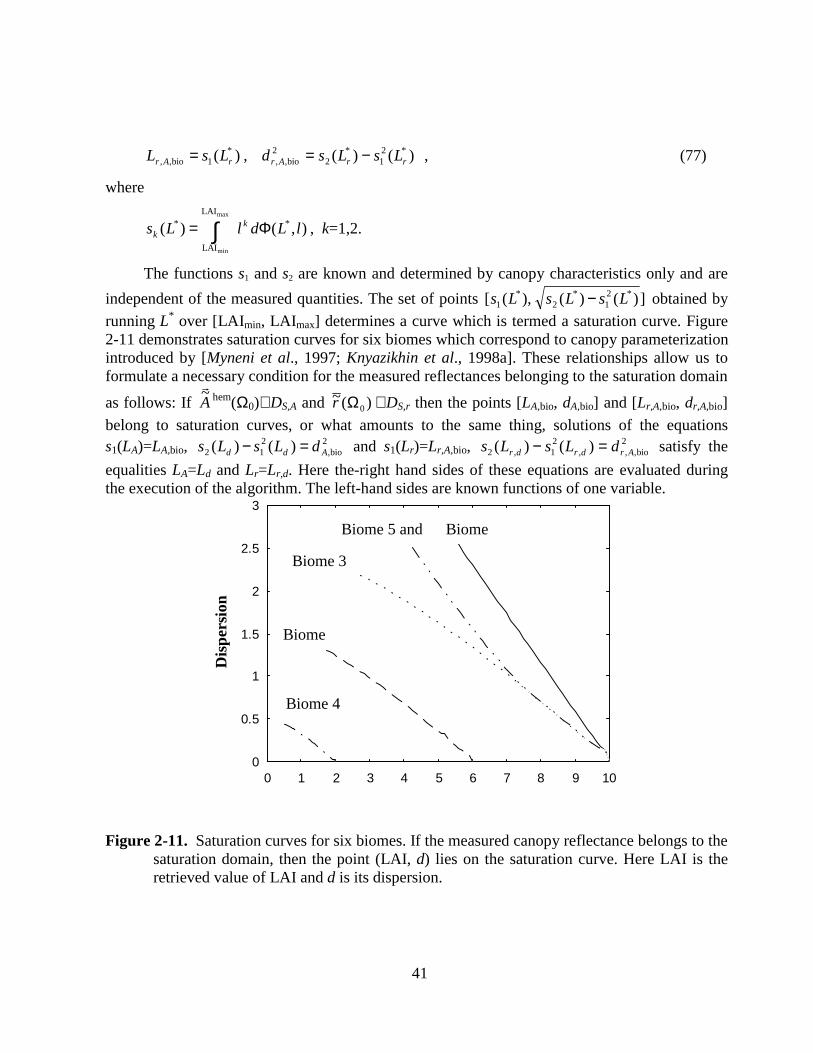
41

)( *1bio,, rAr LsL = , )()( *2

1*

22

bio,, rrAr LsLsd −= , (77)

where

∫ Φ=max

min

LAI

LAI

** ),()( lLdlLs kk , k=1,2.

The functions s1 and s2 are known and determined by canopy characteristics only and are

independent of the measured quantities. The set of points ])()(),([ *21

*2

*1 LsLsLs − obtained by

running L* over [LAImin, LAImax] determines a curve which is termed a saturation curve. Figure2-11 demonstrates saturation curves for six biomes which correspond to canopy parameterizationintroduced by [Myneni et al., 1997; Knyazikhin et al., 1998a]. These relationships allow us toformulate a necessary condition for the measured reflectances belonging to the saturation domain

as follows: If A&~ hem(Ω0)∈DS,A and )(~

0Ωr ∈DS,r then the points [LA,bio, dA,bio] and [Lr,A,bio, dr,A,bio]

belong to saturation curves, or what amounts to the same thing, solutions of the equationss1(LA)=LA,bio,

2bio,

212 )()( Add dLsLs =− and s1(Lr)=Lr,A,bio,

2bio,,,

21,2 )()( Ardrdr dLsLs =− satisfy the

equalities LA=Ld and Lr=Lr,d. Here the-right hand sides of these equations are evaluated duringthe execution of the algorithm. The left-hand sides are known functions of one variable.

0

0.5

1

1.5

2

2.5

3

0 1 2 3 4 5 6 7 8 9 10

Figure 2-11. Saturation curves for six biomes. If the measured canopy reflectance belongs to thesaturation domain, then the point (LAI, d) lies on the saturation curve. Here LAI is theretrieved value of LAI and d is its dispersion.

Dis

pers

ion

BiomeBiome 5 and

Biome 3

Biome

Biome 4

42

This criterion takes a simple form in the case of biome 1. It follows from (75) and gmin=gmax=1 that the solution distribution function for the saturation domain in these biomes is

≤

<≤−

−

<

=Φ

.LAIif,1

,LAIif,LAI

,if,0

),(

max

max*

*max

*

*

*

L

LLL

LL

LL

LL

Equation (76) is reduced to

2

LAI)( max

**

bio,

+= AAA

LLL , ( )2*

max*2

bio, LAI12

1)( AAA LLd −=

and (77) can be simplified to a similar expression, with *AL replaced by *

rL . After obvioustransformations, one can express the saturation criterion for biomes 1 as follows: If

A&~ hem(Ω0)∈DS,A and )(~

0Ωr ∈DS,r, then

maxbio,bio, LAI3 =⋅+ AA dL and/or maxbio,,bio,, LAI3 =⋅+ ArAr dL (78)

where LA,bio, dA,bio, Lr,A,bio, and dr,A,bio are evaluated from (66), (67), (68), and (69). Thus after theevaluation of LAIs and their variances, condition (78) is checked. We archive -dA,bio and -dr,A,bio

if (78) is satisfied to a given accuracy. Inclusion of the minus sign means that a solution LAI wasfound, but the value probably belongs to the saturation domain and any value of LAI from[2⋅LAI - LAI max,LAI max] must be considered as a true solution with equal probability.

Other biome types do not allow for the formulation of the saturation criteria in a suchsimple form. Therefore we store saturation curves for all biomes in the look-up table. Afterevaluation of LAIs from (66) and (67) and their variances from (68) and (69), conditionsm(dA,bio,LA,bio)=0 and m(dr,A,bio,Lr,A,bio)=0 are checked. Here

])()([])([min),( 2*21

*2

2*1

LAILAI max*

min

dLsLsLLsLdmL

−−+−=≤≤

. (79)

We archive -dA,bio and -dr,A,bio if these relationships are fulfilled to a given accuracy.

2.10 Description of FPAR Retrieval

It follows from (29) and (32) that the fractional amount of incident photosyntheticallyactive radiation (PAR) absorbed by the vegetation canopy (FPAR) can be evaluated as

),,(),,()()(),(FPAR 00

700nm

nm400

0hem Ω+Ω=Ω= ∫ pbioQLAIbioQdepbio q

bsλλλa , (80)

where

∫ Ω=Ω700nm

nm400

0hem

,0bs )()(),,( λλλ deLAIbioQ bsa , (81)

43

∫ −Ω=Ω

700nm

nm400

,hem,bs

,eff,

eff,0,0 )(

)(1

)()(),,( λλ

λρλρ

λλ

λ depbioQ q

qq

qq

q tr

a (82)

[ ]∫ Ω−ΩΩΩ

=700nm

nm400

0hem

,bs0hem

0,

0, )()()(~

)(

)(λλλλ

λ

λ deAq

q rt

a . (83)

The Qbs term describes the absorption within the canopy for a black-soil condition, and Qq termdescribes the additional absorption within the canopy due to the interaction between theground (soil and/or understory) and the canopy. Here p∈Pbio; e is the ratio of themonochromatic flux incident at the top surface of the canopy boundary to the totaldownward PAR flux which can be expressed as

∫ Ω

Ω= 700nm

nm400

0hem

,0

0hem

,0

)(

)()(

λλ

λλ

λλ

deE

eEe ,

where E0,λ is the solar irradiance spectrum that is known for all wavelengths; hemλe is the

normalized incident irradiance defined as the ratio of the radiant incident on the surfaceto E0,λ [Diner et al., 1998a]. The mean over those p∈Pbio which passed the test ∆(p)≤h istaken as the estimate of FPAR, i.e.,

∑=

=PN

kPbio pbio

N 1

),(FPAR1

FPAR ,

where NP is the number of canopy realizations p∈Pbio passing this test. When there is no solution(i.e., Fbio=0), the algorithm defaults to a NDVI-FPAR regression analysis to obtain anestimate of FPAR [Myneni et al, 1997b].

The normalized incident irradiance and the BHR are provided by the MISR instrument atthree spectral bands within the PAR region. We assume a piece-wise linear variation in thesevariables over regions [446 , 558 nm], [558, 672 nm], and a constant over regions [400 ,446nm],[672 ,700nm]. Substituting these piece-wise linear functions into (80) and (83), one can express

FPAR as a function of hemλe and hem~

λA [Diner et al., 1998a]. Note that the dependence of FPAR

on ground reflection properties is included in hem~λA which is provided by the MISR instrument;

44

that is, expression (80) is a function of the biome type, Sun position, ground cover, mean leafarea index of an individual plant, and retrieved BHR.

If only MODIS observations are available for a given pixel or the MODIS-only mode isexecuted, e(λ) is approximated by

∫= nm700

nm400

0

0

)5200(

)5200()(

KE

KEe

λ

λλ ,

where Eλ(T) is the Planck function [Kondratyev, 1969, p. 230]. In this case, the Qq term is afunction of the biome type, Sun position, ground cover, mean leaf area index of anindividual plant, and pattern of the effective ground reflectance. Expression (82) is usedto evaluate this term. The Qbs and Qq terms are precomputed and stored in the look-uptable.

2.11 Theoretical Basis of NDVI-FPAR RelationsThe measured spectral reflectance data are usually compressed into vegetation indexes.

More than a dozen such indexes are reported in the literature and shown to correlate well withvegetation amount [Tucker, 1979], the fraction of absorbed photosynthetically active radiation[Asrar et al., 1984], unstressed vegetation conductance and photosynthetic capacity [Sellers etal., 1992], and seasonal atmospheric carbon dioxide variations [Tucker et al., 1986]. There aresome theoretical investigations to explain these empirical regularities [Vygodskaya andGorshkova, 1987; Myneni et al., 1995a; Verstraete and Pinty, 1996]. Results from the previoussection allow us to relate the vegetation indexes to the fundamental physical principle, i.e., thelaw of energy conservation. Here we consider the normalized difference vegetation index(NDVI) whose use is included in the LAI/FPAR retrieval algorithm.

Let us consider NDVI defined as

hemhem

hemhem

NDVIβα

βα

AA

AA

+−

= , (84)

where hemλA is the BHR or DHR, and α and β are near-IR and red spectral wavebands,

respectively. These variables are a function of Sun position Ω0, but this dependence hasbeen suppressed in the notation of this section. For the sake of simplicity, we consider theNDVI for the “black-soil” problem and “S problem.” It follows from equations (54), (53),and (52) that equation (84) can be rewritten as

)(),()(),()(2

)(),()(),(NDVI

ββαββαβββαββα

tarta

mk

mk

−+−= . (85)

where

45

)(1

)(1

)(1

)(11),(

,0

,0

βωαω

αγβγ

βα−−⋅

−−

−=a

ak , 1)(1

)(1),(

,0

,0 −−−

=αγβγ

βαt

tm .

Here γ0,a and γ0,t are defined by equation (55) with K=Ka (for canopy absorptance) andK=Kt (for canopy transmittance), respectively. Here the ratio between the leaf spectralreflectance and the leaf albedo is assumed to be constant with respect to wavelength, and so it isexcluded from the argument list of t. After simple transformations, one obtains

( )ββθβ ,, ,)(NDVI rta ss⋅= ,

where the function θ has the following form

xmky

xmkyxs

⋅−+⋅−=),(),(2

),(),(),(

βαβαβαβα

,

)(

)(, β

ββ a

tt =s ,

)(

)(, β

ββ a

rr =s .

Thus NDVI is proportional to the canopy absorptance at the red band. It follows from Eqs. (53)and (85) that

),()(1

)(1

)(1

)(1)(

)(1

)(1

)(1

)(1)(

,,,0

,0

,0

,0

ββθβωλω

λγβγ

ββωλω

λγβγ

λrta

a

a

a aass

NDVI

−−

−−

=−−

−−

= .

Let e(λ) be the ratio of monochromatic radiant energy incident on the top surface of thecanopy boundary to the total PAR flux. Integrating e⋅a over the PAR region of solar spectrum,we get

FPAR=k⋅NDVI ,

where

( )

−−

−−

= ∫700

400 ,0

,0

,,

)()(1

)(1

)(1

)(1

,

1 λλλγ

λωβωβγ

θ ββ

dess

ka

a

rt

.

Thus if the canopy ground is ideally black, FPAR is proportional to NDVI. The factor ofproportionality k depends on the ratios st,β and st,β, the coefficients Ka and Kt, and the leafalbedo at the red and near-IR spectral bands. A relationship between NDVI and FPARwhich accounts for the soil contribution can be derived from equation (27) in a similarmanner. Other types of vegetation indexes can be derived in an analogous way.

46

2.12 Backup Algorithm

If there are no candidate biome/canopy models which passed the comparison test for agiven pixel, a back-up algorithm is triggered to estimate LAI and FPAR using NormalizedDifference Vegetation Index (NDVI). This backup algorithm requires a land cover classificationthat is compatible with the radiative transfer model used in their derivation. Such a classificationis expected to be derived from the MODIS Land Cover Product. Backup algorithm usesregression curves to estimate LAI and FPAR values, namely,

LAI = f1(NDVI) , FPAR= f2(NDVI).

Here f1 and f2 are biome dependent regression curves which were derived as described below.

Definition of regression curves. Two curves x(y)=E(X | Y=y) and y(x)=E(Y | X=y) definedin the (x,y)-plane are called the regression curves of X with respect to Y and of Y with respect toX, respectively. Here, X and Y are random variables; E(X | Y=y) is expectation of X under thecondition that Y has taken the value y. The regression curve has the following interpretation: thebest possible prediction of X given a realized value y of Y is x(y). The regression curve x(y)minimizes the expected squared error of the prediction of X on the basis of value of y, and y(x)can be interpreted similarly.

Regression curves were used to build the LAI-NDVI and NDVI-FPAR relationshipsestimated with the MODIS LAI/FPAR algorithm applied to the SeaWiFS data as follows. Thesurface reflectance was treated as a biome dependent random variable. The SeaWiFS data weretaken as the sets of realizations of this random variable. The MODIS LAI/FPAR algorithm isbased on the estimation of the LAI distribution function under the condition that the canopyreflectances at the MODIS spectral bands have taken given values. This allows us to treat valuesof LAI and FPAR as random variables. The LAI/FPAR algorithm was applied to these data inorder to evaluate sets of realizations of LAI and FPAR random values. The sets of NDVIrealizations were obtained from the SeaWiFS data directly. Various regression curves were thenderived using these sets.

Let X, Y, and Z be random variables of LAI, NDVI and FPAR values. Figure 2-12demonstrates realizations of these random variables in the (LAI, NDVI) [left panel] and (NDVI,FPAR) [right panel] planes. We denote the regression curves of LAI with respect to NDVI andof NDVI with respect to LAI by x(y) and y(x), respectively. Similarly, z(y) and y(z) denote thebest possible prediction of FPAR given a realized value y of NDVI and the best possibleprediction of NDVI given a realized value z of FPAR. The regressions curves x(y), y(x), z(y) andy(z) for 6 biomes (Grasses and Cereal Crops; Shrubs, Broadleaf Crops; Savannas; BroadleafForests; Needle Forests) are shown in Figure 2-13. The relationships were taken as f1 and f2,respectively. The regression curves x(y), y(x) and z(y), y(z) for biome 5 (Broadleaf Crops) arepresented in Figure 2-14. One can see that the curves y(x) and z(y) are close to the inversefunction of x(y) and y(z), respectively. This may be taken as evidence of the existence of LAI-NDVI and NDVI-FPAR relationships that have previously been reported in the literature. Table2-2 shows NDVI and corresponding LAI and FPAR values used by the current version of thealgorithm. This table may be updated when MODIS data are available.

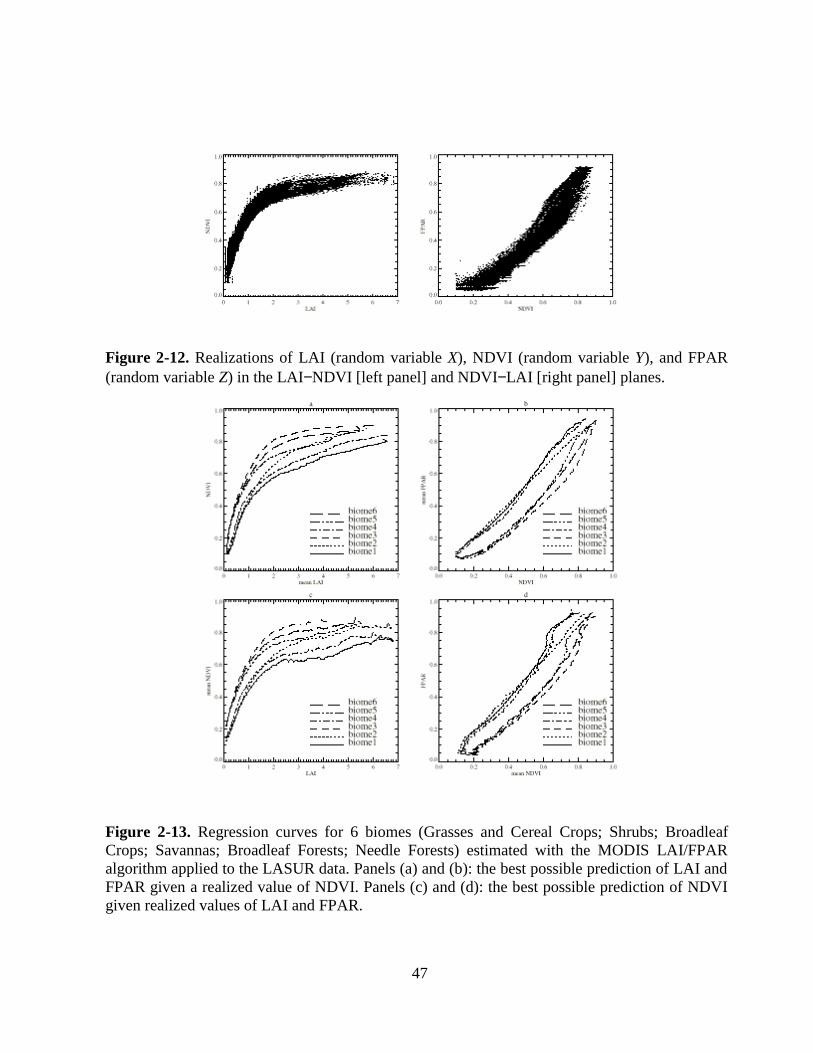
47

Figure 2-12. Realizations of LAI (random variable X), NDVI (random variable Y), and FPAR(random variable Z) in the LAI−NDVI [left panel] and NDVI−LAI [right panel] planes.

Figure 2-13. Regression curves for 6 biomes (Grasses and Cereal Crops; Shrubs; BroadleafCrops; Savannas; Broadleaf Forests; Needle Forests) estimated with the MODIS LAI/FPARalgorithm applied to the LASUR data. Panels (a) and (b): the best possible prediction of LAI andFPAR given a realized value of NDVI. Panels (c) and (d): the best possible prediction of NDVIgiven realized values of LAI and FPAR.

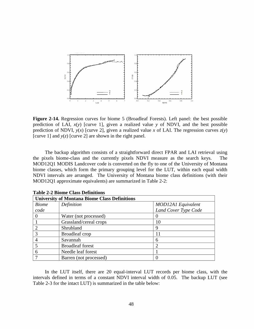
48

Figure 2-14. Regression curves for biome 5 (Broadleaf Forests). Left panel: the best possibleprediction of LAI, x(y) [curve 1], given a realized value y of NDVI, and the best possibleprediction of NDVI, y(x) [curve 2], given a realized value x of LAI. The regression curves z(y)[curve 1] and y(z) [curve 2] are shown in the right panel.

The backup algorithm consists of a straightforward direct FPAR and LAI retrieval usingthe pixels biome-class and the currently pixels NDVI measure as the search keys. TheMOD12Q1 MODIS Landcover code is converted on the fly to one of the University of Montanabiome classes, which form the primary grouping level for the LUT, within each equal widthNDVI intervals are arranged. The University of Montana biome class definitions (with theirMOD12Q1 approximate equivalents) are summarized in Table 2-2:

Table 2-2 Biome Class DefinitionsUniversity of Montana Biome Class DefinitionsBiomecode

Definition MOD12A1 EquivalentLand Cover Type Code

0 Water (not processed) 01 Grassland/cereal crops 102 Shrubland 93 Broadleaf crop 114 Savannah 65 Broadleaf forest 26 Needle leaf forest 17 Barren (not processed) 0

In the LUT itself, there are 20 equal-interval LUT records per biome class, with theintervals defined in terms of a constant NDVI interval width of 0.05. The backup LUT (seeTable 2-3 for the intact LUT) is summarized in the table below:

49

Table 2-3 NDVI and Corresponding Values of LAI and FPAR

Biome1 Biome2 Biome3 Biome4 Biome5 Biome6NDVILAI FPAR LAI FPAR LAI FPAR LAI FPAR LAI FPAR LAI FPAR

0.025 0 0 0 0 0 0 0 0 0 0 0 00.075 0 0 0 0 0 0 0 0 0 0 0 00.125 0.3199 0.1552 0.2663 0.1389 0.2452 0.132 0.2246 0.1179 0.1516 0.07028 0.1579 0.084070.175 0.431 0.2028 0.3456 0.1741 0.3432 0.1774 0.3035 0.1554 0.1973 0.08922 0.2239 0.11590.225 0.5437 0.2457 0.4357 0.2103 0.4451 0.2192 0.4452 0.218 0.2686 0.1187 0.324 0.16180.275 0.6574 0.2855 0.5213 0.2453 0.5463 0.2606 0.574 0.2731 0.3732 0.1619 0.4393 0.21210.325 0.7827 0.3283 0.6057 0.2795 0.6621 0.3091 0.7378 0.3395 0.5034 0.2141 0.5629 0.26240.375 0.931 0.3758 0.6951 0.3166 0.7813 0.3574 0.878 0.393 0.6475 0.2714 0.664 0.30280.425 1.084 0.419 0.8028 0.3609 0.8868 0.3977 1.015 0.4425 0.7641 0.32 0.7218 0.3330.475 1.229 0.4578 0.9313 0.4133 0.9978 0.4357 1.148 0.4839 0.9166 0.3842 0.8812 0.3930.525 1.43 0.5045 1.102 0.4735 1.124 0.4754 1.338 0.5315 1.091 0.4402 1.086 0.45990.575 1.825 0.571 1.31 0.535 1.268 0.5163 1.575 0.5846 1.305 0.4922 1.381 0.54070.625 2.692 0.6718 1.598 0.6039 1.474 0.566 1.956 0.6437 1.683 0.568 1.899 0.64580.675 4.299 0.8022 1.932 0.666 1.739 0.6157 2.535 0.6991 2.636 0.702 2.575 0.73980.725 5.362 0.8601 2.466 0.7388 2.738 0.7197 4.483 0.8336 3.557 0.7852 3.298 0.81070.775 5.903 0.8785 3.426 0.822 5.349 0.8852 5.605 0.8913 4.761 0.8431 4.042 0.85660.825 6.606 0.9 4.638 0.8722 6.062 0.9081 5.777 0.8972 5.52 0.8697 5.303 0.89640.875 6.606 0.9 6.328 0.9074 6.543 0.9196 6.494 0.9169 6.091 0.8853 6.501 0.91950.925 6.606 0.9 6.328 0.9074 6.543 0.9196 6.494 0.9169 6.091 0.8853 6.501 0.91950.975 6.606 0.9 6.328 0.9074 6.543 0.9196 6.494 0.9169 6.091 0.8853 6.501 0.9195

50

3. Algorithm Prototyping

The objectives of this section are: by prototyping the MODIS LAI/FPAR algorithm withatmospherically corrected AVHRR (LASUR) and Landsat data to assess the effect ofuncertainties in surface reflectance data on the quality of the LAI/FPAR product; to analyzeglobal LAI/FPAR fields derived with the algorithm from LASUR data; to analyze the situationsand reasons when the algorithm fails; and to understand the behavior of the algorithm as afunction of spatial resolution.

3.1 Data Analysis

Before MODIS data are available, data acquired by other instruments can be used toprototype and test the functionality of the LAI-FPAR algorithm. The aim of this section is todescribe and analyze the surface reflectance data used to prototype the algorithm.

3.1.1 Satellite Data

LASUR (LAnd SUrface Reflectances) is data acquired during 1989-1990 and processedat Centre d'Etudes Spatiales de la BIOsphere (CESBIO), France from the Advanced Very HighResolution Radiometer (AVHRR) onboard the NOAA 11 satellite. AVHRR is a cross-trackscanning system featuring one visible (RED, 572-698 nm), one NIR (716-985 nm), one shortwave infrared and two thermal infrared channels. For LASUR products, data from RED andNIR channels were used to estimate surface reflectances and vegetation index, and data from thetwo thermal infrared channels were used to estimate the surface temperature. LASUR data werecalibrated and corrected for atmospheric effects and filtered to eliminate residual noises andperturbations. The data span from 75o N to 55o S in latitude, and 180o W to 180o E inlongitude. Each image has 904 rows and 2500 columns. The spatial resolution is 1/7th degree.The temporal resolution is weekly. In this study, RED and NIR surface reflectances from July,1989 were used to prototype the MODIS LAI/FPAR algorithm. We created a monthly layerbased on maximum NDVI compositing of the four weekly layers in this month. By doing so,cloud contamination, off-nadir viewing effects, sun-angle and shadow effects, aerosol and water-vapor effects can be minimized [Holben, 1986].

A Biome Classification Map (BCM) that describes the global distribution of six canopystructural types (biomes) was used as a prototype of the MODIS Land Cover Product, which isrequired by the MODIS LAI/FPAR algorithm. This data set was derived from the AVHRRPathfinder data set [Myneni et al., 1997] and it is a time-independent data set. These biometypes are: grasses and cereal crops (biome 1), shrubs (biome 2), broadleaf crops (biome 3),savannas (biome 4), broadleaf forests (biome 5), and needle forests (biome 6).

We also utilized Landsat Thematic Mapper (TM) scenes of Northwest U. S.(Washington and Oregon) from June 26, 1987 at 30 meter resolution in this study to evaluate thealgorithm response to high resolution data. The data are of 6 spectral bands, bands 1, 2, 3, 4, 5and 7. This image was geometrically registered to a terrain-corrected image with an UTM(Universal Transverse Mercator) projection. The dark object subtraction method of atmosphericcorrection was used to correct surface reflectance for the atmospheric effect. There was also a

51

"sitemap", containing polygons of known ground cover, associated with this data set. Thissitemap distinguishes 17 different forest densities, based on percent forest cover in a forestedpixel, and 7 other types of miscellaneous landcover types. By using the Bayesian Maximumlikelihood classification method, we separated three biomes in this Landsat image, namely,grasses and cereal crops, broadleaf and needle forests. Agriculture (crop, pasture) class wastaken as biome 1. We attribute to broadleaf forests all the pixels in which hardwood forestmakes up more than 60% of the area in one pixel. Needle forests consist of those pixels in whichconifer forest makes up more than 60% of the area in one pixel. The other landcover classes notbelonging to these three biomes were all defined as unknown class type. In all, grasses occupy6.6% of the total area, and broadleaf and needle forests occupy 4.8% and 10.3% of the total area.

3.1.2 Spectral Signatures

Although all the vegetation types have relatively similar spectral properties--largeabsorption in RED and large reflectance in NIR, different biomes have special characteristicsdepending on the canopy architecture. These can be distinguished by comparing their spectralsignatures. Figure 3-1(a), (b) presents histograms of canopy reflectances in RED and NIRspectral bands as a function of biome type derived from the LASUR data. In the RED band,canopy reflectances vary between 0.0 and 0.2. Broadleaf and needle forests have the strongestabsorption features. On an average, they reflect only 3% and 4.5% (Table I) of the incoming

TABLE 3-1 SPECTRAL CHARACTERS OF DIFFERENT VEGETATION TYPES FOR LASUR DATA AND LANDSAT TM DATA

LASUR DATA

Biome Type Mean Red Mean NIR Mean NDVIGrasses and Cereal Crops 0.080 0.25 0.515

Shrubs 0.050 0.21 0.615Broadleaf Crops 0.065 0.32 0.662

Savanna 0.050 0.23 0.645Broadleaf Forests 0.030 0.29 0.813

Needle Forests 0.045 0.25 0.695

LANDSAT DATA

Biome Type Mean Red Mean NIR Mean NDVIGrasses and Cereal Crops 0.065 0.304 0.635

Broadleaf Forests 0.022 0.348 0.881Needle Forests 0.013 0.200 0.886

** The LASUR data is July 1989 globally, which is composited from four weeks data using maximum NDVI.The Landsat TM data is from June 26, 1987, which is a scene of Northwest U.S. (Washington and Oregon).

52

Figure 3-1 Histogram of canopy reflectances for global LASUR data in July 1989 at (a) REDband, (b) NIR band. (c) histogram of NDVI. The interval is 0.25 for above three variables. (d)25% density contours in RED-NIR space, which shows the location of points with high densityfor different biomes.

radiation. Grasses and broadleaf crops are characterized as the brightest biomes; about 8% and6.5% of the incoming radiation is reflected. In the NIR band, reflectances vary between 0.1 and0.5. Shrubs and broadleaf crops represent the extremes. Their reflectances, on an average, are21% and 32%, respectively. The other biomes reflect about 25% of the incoming radiation andthe histograms are similar.

Vegetation indices typically capture the absorption contrast across the 0.65-0.85 mµwavelength interval through combinations of broad-band RED and NIR reflectance. The mostwidely used index in the processing of satellite data is the Normalized Difference VegetationIndex (NDVI) defined as ( ) ( )[ ]RNRN / ρ+ρρ−ρ , where Nρ and Rρ are spectral reflectance at

NIR and RED wavelengths, respectively. NDVI is a measure of chlorophyll abundance and

53

energy absorption [Myneni et al., 1995]. Figure 3-1(c) demonstrates the distribution of NDVIvalues derived from the LASUR data. In general, broadleaf forests have the highest NDVIvalues (0.813), followed by needle forest (0.695). Broadleaf crops and savannas have similarNDVI distributions, and their NDVI values are larger than those of grasses (0.515) and shrubs(0.615). Obviously, it would be difficult to distinguish broadleaf crops from savannas usingNDVI only.

The data density distribution function, introduced earlier in Section II, can be used toindicate the location of data peak in the spectral space. Figure 3-1(d) shows the location ofpoints with high density for different biomes in the RED-NIR space. Each area bounded by thecontour represents an area containing the 25% density of pixels from a given biome type. Wecan see that the biomes tend to cluster and occupy certain well localized spaces. Broadleafforests are located at low RED and high NIR area, while grasses at the high RED and low NIRarea. Broadleaf crops and savannas occupy different locations although their NDVI distributionsare comparable, not surprisingly because NDVI is a non-linear function of RED-NIRreflectances. We also note that some biomes overlap considerably. In general, the more uniquethe location, the better the ability to distinguish them. The influence of soil is also clear fromthis panel. Grasses and shrubs are biomes that are located near the soil line. Broadleaf forestsare a dense vegetation type and these are located closest to the NIR axis.

Figure 3-2 presents canopy reflectance features from Landsat data. On an average,grasses, broadleaf and needle forests reflect only 6.5%, 2% and 1.3% of the incoming radiationin the RED band. This is much less than that of LASUR data. On the other hand, the NIRreflectance of grasses and broadleaf forest can be as high as 30% and 34.8%, compared with25% and 29% for the LASUR data. Needle forests are the darkest among the three biomes, bothat RED and NIR. The NDVI values for the three biomes are 0.635, 0.881, 0.886, respectively.The 25% density contours are tightly clustered occupying a small but unique location in thespectral space. At the same time, the clusters are away from the soil line, and closer to the NIRaxis. The biomes are so well separated that they do not overlap even on the 75 % densitycontour.

Reflectances decrease in the RED band and increase in the NIR band as spatial resolutionincreases. The effect of soil becomes important when resolution decreases, that is, pixels locatednear the NIR axis (Landsat data) will move towards the soil line (LASUR data). The clusteringof data also depends on resolution: the coarser the resolution, the more the biomes overlap in thetwo dimensional spectral space. Biomes that separate well are unlikely to be misclassified. Onthe other hand, biomes that overlap may be misclassified, and this thus directs the algorithm tothe wrong LUT. The same input data (Red and NIR reflectances) will result in differentLAI/FPAR values because the algorithm is biome dependent.

54

3.2 Prototyping of The Algorithm

3.2.1 Prototyping with LASUR Data

This section describes results of global LAI and FPAR fields derived with the MODISLAI/FPAR algorithm using the LASUR-AVHRR data. The objectives were to analyze theglobal LAI/FPAR fields, and the situations when the algorithm failed, and to assess the influenceof uncertainties in surface reflectances on the quality of the LAI/FPAR product.

The algorithm was run pixel-by-pixel using LASUR and land cover BCM data, on allpixels with NDVI greater than 0.1. The following notions are used in the discussion onalgorithm performance: (1) A pixel for which the algorithm retrieves a value of LAI and FPARis termed as a "retrieved" pixel; (2) A pixel for which the algorithm fails is termed as an "non-retrieved" pixel; (3) The ratio of the number of retrieved pixels to the total number of pixels isnamed the Retrieval Index (RI). All results are reported on biomes.

Figure 3-2 The same as Figure 3-1, but for Landsat TM data, June 1987

55

1) Input Data: Atmospherically corrected surface reflectances and uncertainties inmeasurements and simulations are inputs to the algorithm. However, LASUR reports noinformation on the uncertainties in reflectances. Therefore, the uncertainties were simulated as

[ ] 2/12NIR

2REDNIRRED dd +ε=δ=δ (3.1)

Here ε is the mean uncertainty, which is assumed to be a constant in this study. Figure 3-3demonstrates the dependence of the RI on ε . The RI increases with increase in ε , however, thequality of retrieved LAI/FPAR decreases with increase in ε. If ε is underestimated, thealgorithm fails when real uncertainties in surface reflectances are greater than those determinedby equation (3.1). If ε is overestimated, the algorithm can produce LAI/FPAR values for non-vegetated pixels also. Therefore, there should be a critical value of ε for which equation (3.1)optimally approximates real uncertainties. A value of 0.2 for ε was found optimal in this studyfor LASUR data. The RI varies with biome types at a constant ε . When ε is 0.2, the RI for the6 biomes are 91.5%, 92.7%, 74.0%, 79.7%, 39.3%, 54.5%, respectively. The reason thatbroadleaf and needle forests have low RI is perhaps because of the dark soil pattern used torepresent effective ground reflectance ( )λρ eff,q . Thus, if a pixel is bright, it was not considered

as a pure broadleaf or needle forest pixel, and the algorithm consequently failed. Low values ofRI are not necessarily indicative of poor performance by the algorithm. For the coarse resolutiondata such as LASUR (1/7th of a degree), the vegetation in the pixel may be a case of mixtures ofdifferent land cover classes. Therefore, biome specific spectral features may be lost. At thepresent time, restricting the algorithm to pure vegetation types retains the ability to discriminatebiome types.

Figure 3-3 The dependence of the Retrieval Index on ε . The ε means uncertainties inmeasurements and simulations.

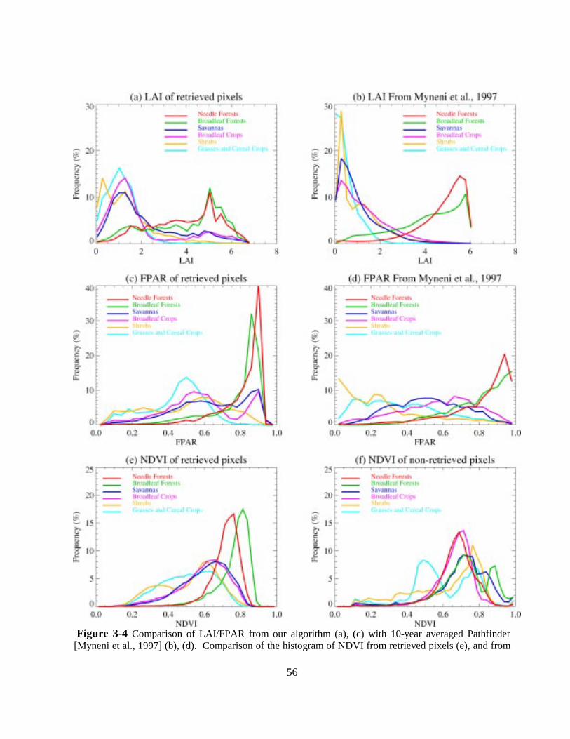
56

Figure 3-4 Comparison of LAI/FPAR from our algorithm (a), (c) with 10-year averaged Pathfinder[Myneni et al., 1997] (b), (d). Comparison of the histogram of NDVI from retrieved pixels (e), and from

57

non-retrieved pixels (f). The mean uncertainty ε used in our algorithm is 0.20 and the interval used forLAI is 0.25, for FPAR and NDVI is 0.04.

2) Histograms of LAI and FPAR: The histogram of the retrieved LAI/FPAR is a statisticalcharacteristic that describes the distribution of these fields for various biomes. Figure 3-4(a)presents the histogram of retrieved LAI using the LASUR data. Broadleaf and needle forestshave distributions distinct from the other four biomes. These biomes have relatively high LAIvalues, concentrated about 4.0 to 6.0. For the other biomes, the LAI values are generally lessthan 2. The differences among grasses, shrubs, broadleaf crops and savannas are seen in thepeak and tail of the LAI histograms. The highest frequency of LAI for broadleaf crops andsavannas is around 1.25, while for grasses it is at 1.0 and for shrubs at 0.75 and 1.25. Forbroadleaf crops and savannas, the tail contains at least 20% of the pixels whose LAI values arelarger than 4.0. On the other hand for grasses and shrubs, the distribution ends at about 4.0.Thus, the mean LAI for broadleaf crops and savannas is 2.1 and 2.2, and for grasses and shrubsonly 1.2 and 1.4. Shrubs have two obvious peaks, which correspond to the two peaks in theNDVI histogram shown in Figure 3-1(c), although the retrieved LAI is not based on the NDVI.

The LAI distribution from a NDVI based algorithm developed earlier by Myneni et al.[Myneni et al., 1997] is shown in Fig 3-4 (b). The data used for this NDVI based algorithm wereAVHRR from July 1981 through June 1991. The average July retrievals over the 10 yearsperiod are shown in Figure 3-4(b). There are many similarities between Figure 3-4(a) and (b).Broadleaf and needle forests have much higher LAI than that of the other four biomes. Thedouble peak in the case of shrubs is also seen in Figure 3-4(b). The similarity between the tworetrievals imbues confidence in the MODIS algorithm in spite of its complexity. However, itshould also be noted that LAI values of the first four biomes are larger in the case of the MODISalgorithm as compared to the NDVI based algorithm. Similarly, the histograms of FPAR ofdifferent biomes match well with the 10-year climatology (Figure 3-4(c) and (d)).

Figure 3-4(e) and (f) show the NDVI histograms from retrieved and non-retrievedpixels. The NDVI histogram of retrieved pixels is similar to the NDVI histogram of all thepixels. Therefore, the algorithm identifies most of the features in the observed data. The failuresare typically of two cases. First, NDVI is too high for a particular biome. For example, thealgorithm fails to retrieve when the NDVI of grasses is larger than 0.75. In the LUT, there is noinformation for grasses at such values of NDVI. Second, for the same NDVI value, some of thepixels are retrieved pixels, but the others not. The failure of this type is discussed later.

3) Test of Physics: There are many examples in published literature of the strongrelationship between a vegetation index such as NDVI and surface parameters LAI and FPAR[Asrar et al., 1984; Tucker et al., 1986; Peterson et al., 1987; Verma et al. 1993; Myneni et al.,1994; Chen, 1996; Chen et al., 1996]. This provides us an opportunity to test the physics of thealgorithm by comparing the LAI-NDVI and FPAR-NDVI relationships derived from thealgorithm with those reported from field measurements. Figure 3-5(a) and (b) show thedistributions of the retrieved values of LAI and FPAR with respect to the NDVI of biome 5. LAIis nonlinearly proportional to NDVI, and FPAR linearly to NDVI. This corresponds to relationsreported in the literature [Myneni et al., 1997; Clevers, 1989]. Note that the NDVI in this plot is

58

evaluated from measured RED and NIR reflectances, while the retrieved quantities result fromthe algorithm which uses reflectances and not NDVI. The advantages of using the MODISalgorithm as opposed to NDVI relations are -- (1) NDVI/LAI relations are subject to changes insun angle, background reflectance, and view angle, while the MODIS algorithm actually usesthese changes as sources of information in the process of retrieval; (2) NDVI is based on twospectral bands only, while the algorithm can ingest 3, 4 or even 7 bands simultaneously toretrieve LAI and FPAR.

Figure 3-5 For broadleaf forests of LASUR data, the scatter plot shows (a) the LAI-NDVIrelationship, (b) NDVI-FPAR relationship, (c) retrieved pixels in RED-NIR space, and (d) non-retrieved pixels in RED-NIR space.

Figure 3-5(e) and (f) show the scatter plot of the data from successful and unsuccessfulpixels in the RED-NIR plane. This distribution provides insight on where and why the algorithmfailed. For retrieved pixels in the RED-NIR plane, canopy reflectances range about 0.02--0.16

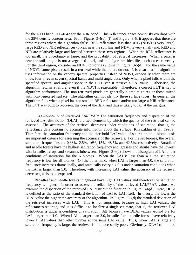
59

for the RED band, 0.1--0.42 for the NIR band. This reflectance space obviously overlaps withthe 25% density contour area. From Figure 3-4(e), (f) and Figure 3-5, it appears that there arethree regions where the algorithm fails: RED reflectance less than 0.03 (NDVI is very large),large RED and NIR reflectances (pixels near the soil line and NDVI is very small) and, RED andNIR are relatively large and located between these two regions. When the RED reflectance istoo small, the uncertainty is large, and the probability of retrieval decreases. When a pixel isnear the soil line, it is not a vegetated pixel, and the algorithm identifies such cases correctly.For the third region, consider an NDVI contour as shown in Figure 3-5(d). For the same valueof NDVI, some pixels result in a retrieval while the others do not. It is clear that the algorithmuses information on the canopy spectral properties instead of NDVI, especially when there arethree, four or even seven spectral bands and multi-angle data. Only when a pixel falls within thespecified spectral and angular space in the LUT, can it retrieve a LAI value. Otherwise, thealgorithm returns a failure, even if the NDVI is reasonable. Therefore, a correct LUT is key toalgorithm performance. The non-retrieved pixels are generally biome mixtures or those mixedwith non-vegetated surface. The algorithm can not identify these surface types. In general, thealgorithm fails when a pixel has too small a RED reflectance and/or too large a NIR reflectance.The LUT was built to represent the core of the data, and thus is likely to fail at the margins.

4) Reliability of Retrieved LAI/FPAR: The saturation frequency and dispersion of theretrieved LAI distribution (DLAI) are two elements by which the quality of the retrieval can beassessed. The accuracy of the retrieval decreases under conditions of saturation, that is, thereflectance data contain no accurate information about the surface [Knyazikhin et al., 1998a].Therefore, the saturation frequency and the threshold LAI value of saturation on a biome basisare important criteria for assessing the accuracy of the retrievals. For the six biomes, the overallsaturation frequencies are 0.38%, 2.5%, 16%, 15%, 48.5% and 42.5%, respectively. Broadleafand needle forests have the highest saturation frequency and, grasses and shrubs have the lowest,with broadleaf crops and savannas inbetween. Figure 3-6(c) shows the histogram of LAI underconditions of saturation for the 6 biomes. When the LAI is less than 4.0, the saturationfrequency is low for all biomes. On the other hand, when LAI is larger than 4.0, the saturationfrequency increases dramatically, and practically every pixel is under saturation conditions whenthe LAI is larger than 5.0. Therefore, with increasing LAI value, the accuracy of the retrievaldecreases, as is to be expected.

Broadleaf and needle forests in general have high LAI values and therefore the saturationfrequency is higher. In order to assess the reliability of the retrieved LAI/FPAR values, weexamine the dispersion of the retrieved LAI distribution function in Figure 3-6(d). Here, DLAIis defined as the ratio of the standard deviation of LAI to LAI itself. In theory, the lower theDLAI value the higher the accuracy of the algorithm. In Figure 3-6(d) the standard deviation ofthe retrieval increases with LAI. This is not surprising, because at high LAI values, thereflectances saturate, and it is difficult to localize a single estimate, that is, the retrieved LAIdistribution is under a condition of saturation. All biomes have DLAI values around 0.2 forLAIs larger than 1.0. When LAI is larger than 3.0, broadleaf and needle forests have relativelylower DLAI values than other biomes at the same LAI value. Thus, when LAI is large andsaturation frequency is large, the retrieval is not necessarily poor. Obviously, DLAI can not be

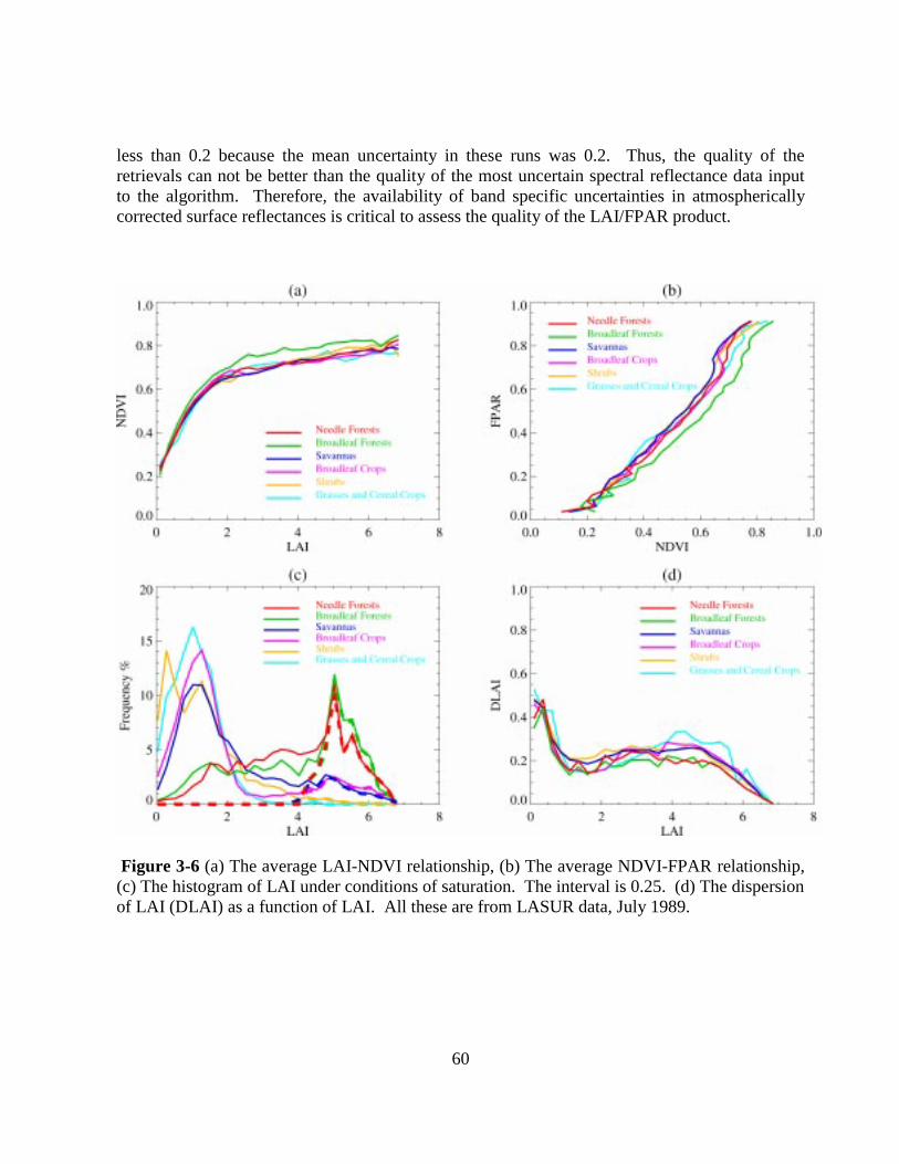
60

less than 0.2 because the mean uncertainty in these runs was 0.2. Thus, the quality of theretrievals can not be better than the quality of the most uncertain spectral reflectance data inputto the algorithm. Therefore, the availability of band specific uncertainties in atmosphericallycorrected surface reflectances is critical to assess the quality of the LAI/FPAR product.

Figure 3-6 (a) The average LAI-NDVI relationship, (b) The average NDVI-FPAR relationship,(c) The histogram of LAI under conditions of saturation. The interval is 0.25. (d) The dispersionof LAI (DLAI) as a function of LAI. All these are from LASUR data, July 1989.

61

5) LAI and FPAR Images: The algorithm was run on the global LASUR data for the month ofJuly 1989. For the unsuccessful pixels, the NDVI-LAI, NDVI-FPAR relations shown in Figure3-6(a) and 6(b) were used to estimate LAI and FPAR. Figure 3-7 shows color-coded images ofglobal LAI and FPAR. These compare well with the fields reported earlier by Myneni et al.[Myneni et al., 1997].

(a)

(b)

Figure 3-7 Global (a) LAI and (b) FPAR derived from LASUR data in July, 1989. Thealgorithm was run on LASUR data. For the non-retrieved pixels, the LAI-NDVI, NDVI-FPARrelations shown in Figure 6(a) and (b) were used to estimate LAI and FPAR.

62

6) Biome Misclassification and LAI/FPAR Retrievals: It is important to assess theimpact of biome misclassification on LAI/FPAR retrievals. To understand this, we ran algorithm6 times per pixel, each time with a different biome's LUT. This simulates the effects of biomemisclassification on LAI/FPAR retrievals. The results are shown in Table II and Figure 3-8.For example, for grasses and cereal crops ( Figure 3-8(a)), the histogram of grasses and cerealcrops indicates that pixels of this vegetation type were retrieved using the correct LUT; thehistogram of shrubs indicates that pixels of this vegetation type were misclassified as shrubs andwere therefore retrieved using the LUT for the shrubs vegetation type.

When pixels are misclassified, typically, either the Retrieval Index (RI) is low and/or theretrieved LAI values are incorrect. When misclassification between clearly distinct biomeshappens, the results are predictable. Consider grasses and cereal crops (biome 1) and broadleafforests (biome 5), which are distinct in their architecture and foliage optics. When biome 1 ismisclassfied as biome 5, the RI is only 27% compared to 91% without misclassification. Whenbiome 5 is misclassified to biome 1, the retrieved LAI value decreases from 4 or 5 to 2. Thus,misclassification can be detected by RI, mean LAI and the histogram of the retrieved LAIdistribution. On the other hand, when misclassification happens between spectrally andstructurally similar biomes, perhaps because of coarse spatial resolution, the impact onLAI/FPAR retrievals is difficult to assess. As an example, consider shrubs (biome 2) andsavannas (biome 4). The RI does not change much, and the mean LAI is also similar. Thus, theretrieved LAI/FPAR values are acceptable, although the pixels have been misclassified. Such acase also indicates that the various biome LUTs share similar entries for certain combinations ofspectral reflectances.

3.2.2 Prototyping With Landsat Data

1) General Results: The MODIS LAI/FPAR algorithm was also prototyped withLandsat data for three biomes (grasses and cereal crops, broadleaf forests, needle forests) asmentioned previously. A fine resolution LUT was used to retrieve LAI and FPAR because of thefiner spatial resolution of the Landsat data. The RI for the three biomes was 90.7%, 53.9%,57.9%, respectively, and the mean LAI values were 1.87, 5.79, 4.11. Compared to LASUR data,not only did the RI increase for broadleaf and needle forests, but also the mean LAI valueincreased. The finer resolution pixels contain fewer mixtures which perhaps explains theseresults. The saturation frequencies at high LAI values for the three biomes are comparable tothose reported earlier for the LASUR data, but the dispersions (DLAI) are narrower for broadleafand needle forests indicating a better localization of the retrievals. Thus, compared to coarseresolution data, the 30 m resolution Landsat data result in qualitatively better retrievals of LAIand FPAR. This highlights the value of spatial resolution and indicates that the 1 km MODISLAI/FPAR retrievals will be better accurate than the 8 km AVHRR retrievals currently available.

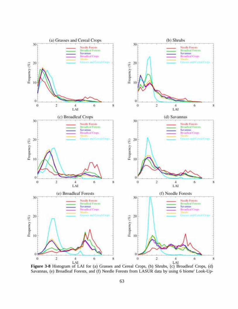
63

Figure 3-8 Histogram of LAI for (a) Grasses and Cereal Crops, (b) Shrubs, (c) Broadleaf Crops, (d)Savannas, (e) Broadleaf Forests, and (f) Needle Forests from LASUR data by using 6 biome' Look-Up-

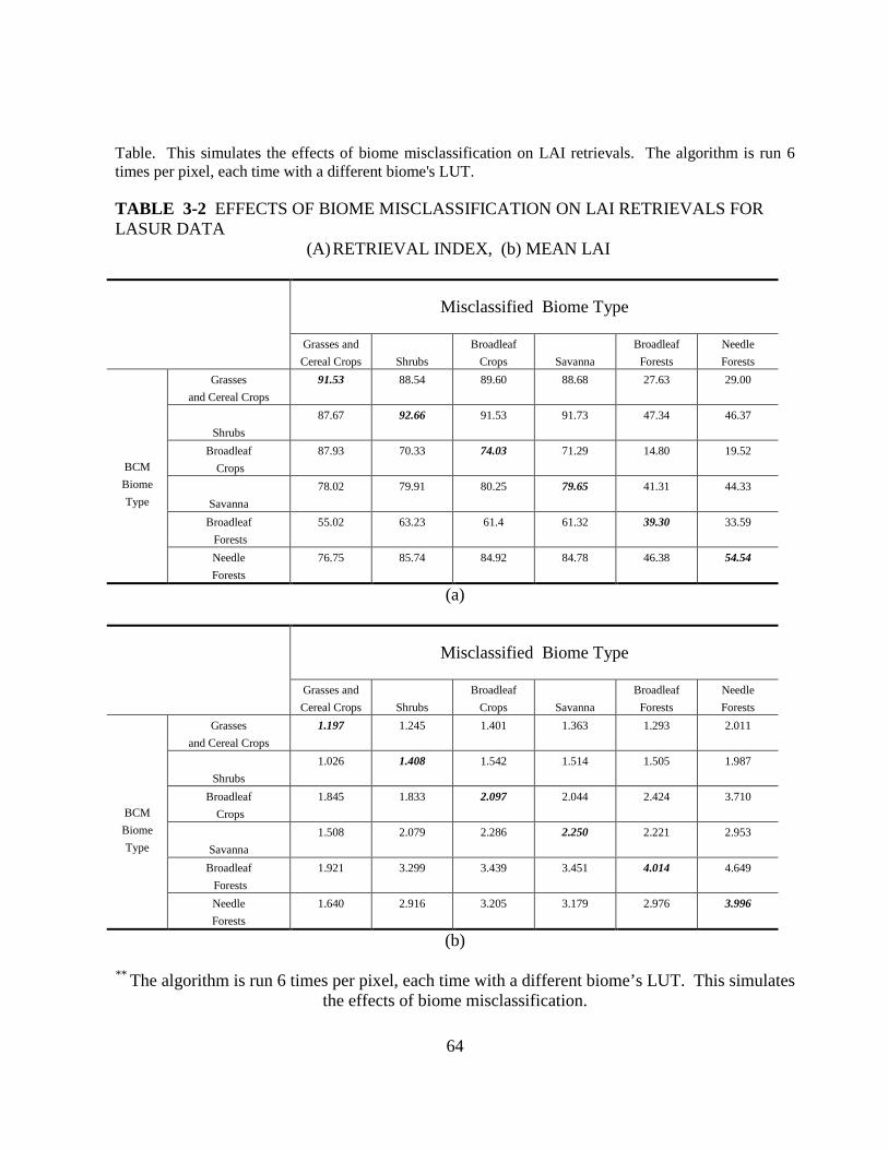
64

Table. This simulates the effects of biome misclassification on LAI retrievals. The algorithm is run 6times per pixel, each time with a different biome's LUT.

TABLE 3-2 EFFECTS OF BIOME MISCLASSIFICATION ON LAI RETRIEVALS FORLASUR DATA

(A) RETRIEVAL INDEX, (b) MEAN LAI

Misclassified Biome Type

Grasses and

Cereal Crops Shrubs

Broadleaf

Crops Savanna

Broadleaf

Forests

Needle

Forests

Grasses

and Cereal Crops

91.53 88.54 89.60 88.68 27.63 29.00

Shrubs

87.67 92.66 91.53 91.73 47.34 46.37

Broadleaf

Crops

87.93 70.33 74.03 71.29 14.80 19.52

Savanna

78.02 79.91 80.25 79.65 41.31 44.33

Broadleaf

Forests

55.02 63.23 61.4 61.32 39.30 33.59

BCM

Biome

Type

Needle

Forests

76.75 85.74 84.92 84.78 46.38 54.54

(a)

Misclassified Biome Type

Grasses and

Cereal Crops Shrubs

Broadleaf

Crops Savanna

Broadleaf

Forests

Needle

Forests

Grasses

and Cereal Crops

1.197 1.245 1.401 1.363 1.293 2.011

Shrubs

1.026 1.408 1.542 1.514 1.505 1.987

Broadleaf

Crops

1.845 1.833 2.097 2.044 2.424 3.710

Savanna

1.508 2.079 2.286 2.250 2.221 2.953

Broadleaf

Forests

1.921 3.299 3.439 3.451 4.014 4.649

BCM

Biome

Type

Needle

Forests

1.640 2.916 3.205 3.179 2.976 3.996

(b)

** The algorithm is run 6 times per pixel, each time with a different biome’s LUT. This simulatesthe effects of biome misclassification.

65

Figure 3-9 The retrievals from Landsat data as a function of spatial resolution dependent Look-Up-Table (LUT). Histogram of LAI from (a) Landsat LUT, (b) LASUR LUT. Histogram ofFPAR from (c) Landsat LUT, (d) LASUR LUT.

The reason for the dependency of the LUT on spatial resolution is as follows.Depending on the resolution, leaf canopy spectral properties are very different (Figure 3-1 andFigure 3-2). At fine spatial resolution, leaves absorb more in the RED band and also reflectmore in the NIR band. In the RED-NIR plane, Landsat data tend to cluster, and occupy a smallregion nearer to the NIR axis. The LUT should reflect these changes in vegetation canopyspectral properties with changes in resolution. To investigate this further, the algorithm wasexecuted on Landsat data, but with LASUR LUT, that is, fine resolution data with coarseresolution LUT. Figure 3-9 shows the histogram of LAI and FPAR obtained with Landsat dataand LASUR LUT, and also Landsat data with Landsat LUT. When Landsat data and LUT areused, the retrieved LAI values vary from 0.0 to 2.5 for grasses, 5.0 to 7.0 for broadleaf forest,

66

and 1.5 to 6.0 for needle forests (Table III). When LASUR LUT is used with Landsat data, thehistogram of retrieved LAI and FPAR change greatly. The LAI of grasses/cereal crops can be ashigh as 4.0 to 6.0, which is unrealistic. The LAI of needle forests is concentrated between 1.5 to4.0, which is relatively small for this biome. The RI for the three biomes also decrease to 87.5%,39.2%, 4.7%, respectively. When the algorithm is run using LASUR data but Landsat LUT(Figure 3-10), the retrieved LAI and the mean LAI for all biomes decrease. The differencesbetween forests (high LAI) and other biomes (low LAI) disappear. This clearly indicates thedependency between data resolution and the LUT.

TABLE 3-3 Comparison of the Results from LASUR look-up-table (lut) and LANDSATLUT

LASUR DATA

LASUR LUT LANDSAT LUTBiome Type Retrieval Index Mean LAI Retrieval Index Mean LAI

Grasses and Cereal Crops 91.53 1.20 91.6 1.07Shrubs 92.66 1.41 96.4 0.92

Broadleaf Crops 74.03 2.09 80.1 1.17Savanna 79.65 2.25 85.4 1.61

Broadleaf Forests 39.30 4.01 41.8 2.62Needle Forests 54.54 3.99 41.8 1.66

LANDSAT DATA

LANDSAT LUT LASUR LUTBiome Type Retrieval Index Mean LAI Retrieval Index Mean LAI

Grasses and Cereal Crops 90.7 1.87 87.5 3.62Broadleaf Forests 53.9 5.79 39.2 6.21

Needle Forests 57.9 4.11 4.7 3.39

** The algorithm was executed on LASUR data with LASUR LUT and Landsat LUT, and also on Landsat data withLandsat LUT and LASUR LUT. The corresponding Retrieval Index and mean LAI indicate the dependence of thealgorithm (LUT) on spatial resolution.

67

Figure 3-10 The retrievals from LASUR data as a function of spatial resolution dependent Look-Up-Table (LUT). Histogram of LAI from (a) LASUR LUT, (b) Landsat LUT. Histogram ofFPAR from (c) LASUR LUT, (d) Landsat LUT.

2) Soil or Background Effects: As mentioned previously, in the design of the MODISLAI/FPAR algorithm, the three-dimensional radiative transfer problem was split into twoindependent sub-problems. The first, the black soil problem, describes the radiation regimewithin the vegetation canopy for the case of a completely absorbing soil or background beneaththe canopy. The second, the S problem, describe the radiation region of the vegetation canopygenerated by anisotropic heterogeneous sources located at the canopy bottom and thischaracterizes the contribution of the soil or background to the canopy radiation regime. At fineresolutions, the contribution of the S problem is negligible in the case of dense vegetation suchas forests. To test this assumption, we executed the algorithm using only the black soil problemon Landsat data. The RI can be as high as 50.6% (broadleaf forest) and 54.3% (needle forest)using just the black soil problem compared to 53.7% and 57.9% if the contribution from the S

68

problem is added. The histograms of retrieved LAI and FPAR do not change much. Thus, thefine resolution Landsat data represent pure biome types, dense vegetation in this instance, withminimal soil or background effects. For the coarse resolution LASUR data, however, thesuccess index is only 31% and 45% for broadleaf and needle forests when only the black soilproblem is used to retrieve LAI and FPAR. The soil problem is very important in this case,which can also be seen in the location of the data in the RED-NIR space, which results from acombination of the S problem and the black soil problem.

Figure 3-11 Same as Figure 3-2(d), 25% density contours of Landsat TM data on June 30, 1987at (a) 30 m resolution, (b) 240 m resolution, and (c) 510 m resolution The 30 m resolution pixelswere averaged to 240 m and 510 m resolution. A 30 m resolution landcover map was used as thebaseline data set. The coarse resolution map were overlaid on the 30 m class map and the coarsegrid cell was labeled based on the most frequently occurring cover type among the 30 mresolution pixels within that grid.

69

3) Spatial Resolution Effects: The impact of spatial resolution and aggregation of data onthe MODIS LAI/FPAR algorithm was further investigated. The study focused mainly onbroadleaf and needle forests. A 30 m resolution landcover map was used as the baseline data set.This map was used to label a series of coarser resolution maps of the scene produced by anaggregation procedure described below. The 30 m resolution pixels were averaged to 240 m and510 m resolution. Each grid at the 240 m aggregation contained 64 30 m pixels. These wereoverlaid on the 30 m class map and the coarse grid cell was labeled based on the most frequentlyoccurring cover type among the high resolution pixels within that grid. This procedure wasperformed for both resolutions. Here, we use two TM images of the same area, but fromdifferent seasons. One of these is the image mentioned previously (June 27, 1987) and the otheris from September 30, 1987.

Figure 3-12 Same as Figure 3-11, data come from September 30, 1987.

70

From a spectral and NDVI point of view, the biomes change differently as the resolutiondecreases (Table IV(a) and (b)). Consider the June image. As resolution decreases, the REDreflectance of broadleaf forests increases and the NIR simultaneously decreases with the resultthat NDVI decreases. For needle forests, the RED as well as the NIR reflectance increases,consequently, NDVI is unchanged. In the RED-NIR space, these changes can be clearly seen(Figure 3-11). The distance between the three biome decreases, that is, the biomes becomespectrally similar as resolution decreases. The September image shows similar changes (Figure3-12), but the difference between the two images can be attributed to changing seasonality. Thereason why needle forests exhibit such a large seasonal change is perhaps due to the understory[Cihlar et al., 1997]. It is important to note the distinct separation between the three biomes inboth the images, suggesting that seasonal changes do not confound differences between thebiomes. The reason why NIR reflectance in needleaf forests increases with decreasing resolutionis their low NIR reflectance compared to the two other biomes. This is shown in Table I as well.Indeed, the spectral properties of coarse resolution data aggregated from fine resolution are alsoinfluenced by landscape characteristics. But, in general, the RED reflectance increases with theresult that the biomes that tend to move towards the soil line in the RED-NIR space.

TABLE 3-4 MEAN VALUES OF RED, NIR, NDVI AND LAI AT 30 m, 240 m AND 510 mRESOLUTION FOR LANDSAT TM DATA ON (a) JUNE 30, 1987, AND (b) SEPTEMBER30, 1987

30 m * 30 m

Biome Type Mean Red Mean NIR Mean NDVI Mean LAIGrasses and Cereal Crops 0.0655 0.304 0.635 1.87

Broadleaf Forests 0.0215 0.348 0.881 5.79Needle Forests 0.0131 0.200 0.886 4.11

240 m * 240 m

Biome Type Mean Red Mean NIR Mean NDVI Mean LAIGrasses and Cereal Crops 0.0646 0.295 0.635 1.795

Broadleaf Forests 0.0275 0.346 0.853 5.385Needle Forests 0.0141 0.232 0.889 4.488

510 m * 510 m

Biome Type Mean Red Mean NIR Mean NDVI Mean LAIGrasses and Cereal Crops 0.0640 0.291 0.635 1.756

Broadleaf Forests 0.0307 0.342 0.835 5.282Needle Forests 0.0158 0.246 0.883 4.584

(a)

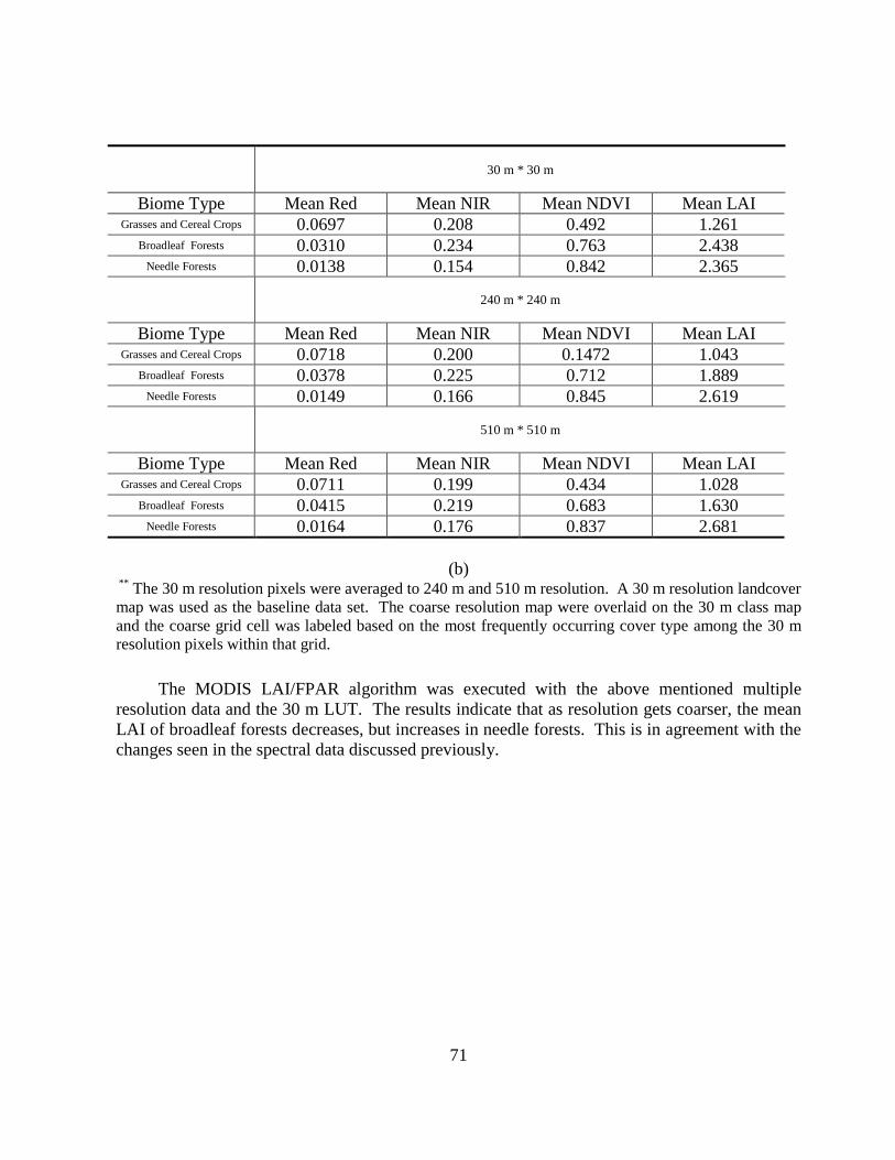
71

30 m * 30 m

Biome Type Mean Red Mean NIR Mean NDVI Mean LAIGrasses and Cereal Crops 0.0697 0.208 0.492 1.261

Broadleaf Forests 0.0310 0.234 0.763 2.438Needle Forests 0.0138 0.154 0.842 2.365

240 m * 240 m

Biome Type Mean Red Mean NIR Mean NDVI Mean LAIGrasses and Cereal Crops 0.0718 0.200 0.1472 1.043

Broadleaf Forests 0.0378 0.225 0.712 1.889Needle Forests 0.0149 0.166 0.845 2.619

510 m * 510 m

Biome Type Mean Red Mean NIR Mean NDVI Mean LAIGrasses and Cereal Crops 0.0711 0.199 0.434 1.028

Broadleaf Forests 0.0415 0.219 0.683 1.630Needle Forests 0.0164 0.176 0.837 2.681

(b) ** The 30 m resolution pixels were averaged to 240 m and 510 m resolution. A 30 m resolution landcovermap was used as the baseline data set. The coarse resolution map were overlaid on the 30 m class mapand the coarse grid cell was labeled based on the most frequently occurring cover type among the 30 mresolution pixels within that grid.

The MODIS LAI/FPAR algorithm was executed with the above mentioned multipleresolution data and the 30 m LUT. The results indicate that as resolution gets coarser, the meanLAI of broadleaf forests decreases, but increases in needle forests. This is in agreement with thechanges seen in the spectral data discussed previously.

72

4 Validation Plan

4.1 Introduction

In July, 1999, NASA will launch the Terra platform, a keystone of its Earth ObservingSystem (EOS). Terra’s five instruments include highly evolved successors to current satellitesensors (e.g., MODIS vs. AVHRR) and innovative experimental sensors (e.g., MISR). Together,the many near real-time products (e.g., leaf area index (LAI)) from Terra will provide the mostcomprehensive view of the Earth system to date. Moreover, the co-aligned, calibrated sensorswill present the best opportunity yet for validation of remote sensing products and algorithms.

Nevertheless, global validation of land remote sensing products is complicated by multiplefactors, including difficulty in measuring land surface variables over the size of a satellite pixel,inherent errors in satellite data calibration, georegistration, cloud screening and atmosphericcorrection, and the impracticality and expense of collecting field data over a large number ofdifferent ground/atmosphere combinations over sufficiently long time scales. These constraintshave therefore limited rigorous validation efforts to several “intensive field campaigns” (e.g.,FIFE, BOREAS, HAPEX) where large teams were able to collect data over reasonably largeareas during discrete phenological periods. While these efforts were necessary to show thatvarious remote sensing algorithms were working correctly, they were not sufficient to trulyvalidate a land product or algorithm, at least not for global, year-round application.

Despite these difficulties, the EOS Project has charged its instrument teams with both thedevelopment and validation of their operational products. In 1998, the Project augmented thoseefforts by funding 65 competitively-selected Validation Investigators. Approximately 44 of thesewill rely on in situ measurements and comparisons with EOS products. Thus, a close dialogue isdeveloping among field data collectors, EOS algorithm developers, and the end-user communityto ensure that the validation data are collected and packaged appropriately for greatesteffectiveness. Particularly notable are the SWAMP Validation Workshop in 1997 [Justice et al.1998] and a 1998 follow-up workshop for LA1 and FPAR (canopy-absorbed radiation)validation [Privette et al. 1998].

4.2 Approach

Multiple validation techniques will be used to develop uncertainty information on EOSland products. The methods include comparisons with in situ data, comparisons with data fromairborne and other spaceborne sensors (e.g., AVHRR, GOES), analysis of trends in products(e.g., spatial, temporal), and analysis of process model (e.g., climate model) results which aredriven or constrained by EOS products. Successful validation will have been accomplished iftimely and accurate product uncertainty information becomes routinely available to the productusers within two years after Terra’s launch.

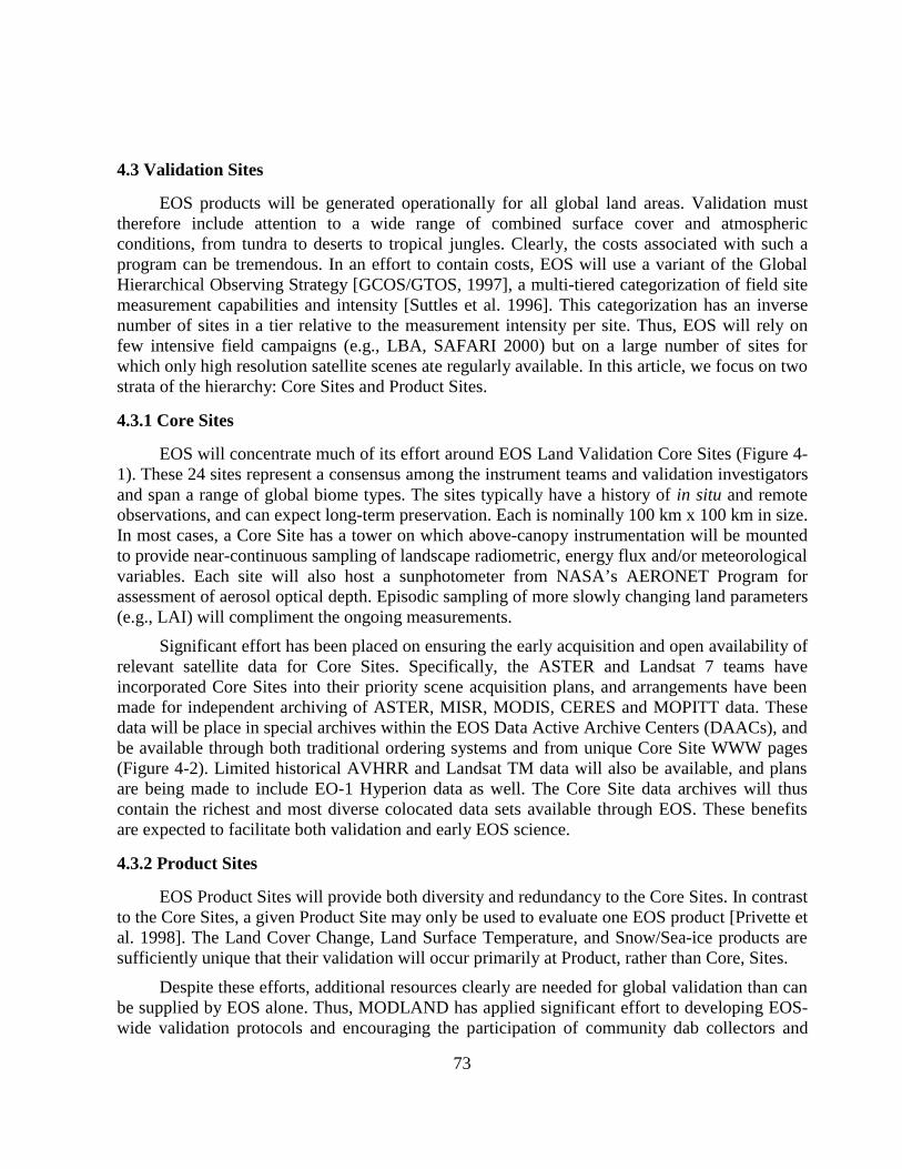
73

4.3 Validation Sites

EOS products will be generated operationally for all global land areas. Validation musttherefore include attention to a wide range of combined surface cover and atmosphericconditions, from tundra to deserts to tropical jungles. Clearly, the costs associated with such aprogram can be tremendous. In an effort to contain costs, EOS will use a variant of the GlobalHierarchical Observing Strategy [GCOS/GTOS, 1997], a multi-tiered categorization of field sitemeasurement capabilities and intensity [Suttles et al. 1996]. This categorization has an inversenumber of sites in a tier relative to the measurement intensity per site. Thus, EOS will rely onfew intensive field campaigns (e.g., LBA, SAFARI 2000) but on a large number of sites forwhich only high resolution satellite scenes ate regularly available. In this article, we focus on twostrata of the hierarchy: Core Sites and Product Sites.

4.3.1 Core Sites

EOS will concentrate much of its effort around EOS Land Validation Core Sites (Figure 4-1). These 24 sites represent a consensus among the instrument teams and validation investigatorsand span a range of global biome types. The sites typically have a history of in situ and remoteobservations, and can expect long-term preservation. Each is nominally 100 km x 100 km in size.In most cases, a Core Site has a tower on which above-canopy instrumentation will be mountedto provide near-continuous sampling of landscape radiometric, energy flux and/or meteorologicalvariables. Each site will also host a sunphotometer from NASA’s AERONET Program forassessment of aerosol optical depth. Episodic sampling of more slowly changing land parameters(e.g., LAI) will compliment the ongoing measurements.

Significant effort has been placed on ensuring the early acquisition and open availability ofrelevant satellite data for Core Sites. Specifically, the ASTER and Landsat 7 teams haveincorporated Core Sites into their priority scene acquisition plans, and arrangements have beenmade for independent archiving of ASTER, MISR, MODIS, CERES and MOPITT data. Thesedata will be place in special archives within the EOS Data Active Archive Centers (DAACs), andbe available through both traditional ordering systems and from unique Core Site WWW pages(Figure 4-2). Limited historical AVHRR and Landsat TM data will also be available, and plansare being made to include EO-1 Hyperion data as well. The Core Site data archives will thuscontain the richest and most diverse colocated data sets available through EOS. These benefitsare expected to facilitate both validation and early EOS science.

4.3.2 Product Sites

EOS Product Sites will provide both diversity and redundancy to the Core Sites. In contrastto the Core Sites, a given Product Site may only be used to evaluate one EOS product [Privette etal. 1998]. The Land Cover Change, Land Surface Temperature, and Snow/Sea-ice products aresufficiently unique that their validation will occur primarily at Product, rather than Core, Sites.

Despite these efforts, additional resources clearly are needed for global validation than canbe supplied by EOS alone. Thus, MODLAND has applied significant effort to developing EOS-wide validation protocols and encouraging the participation of community dab collectors and

74

product users. In particular, significant collaboration is planned with existing measurementnetworks, including FLUXNET, Long Term Ecological Research (LTER) sites, AERONET, andGlobal Land Cover Test Sites (GLTCS). In most cases, the EOS Core Sites are members of atleast one of these networks. In addition, EOS is investigating the potential usefulness of othernetworks, such as BSRN and SurfRad.

Figure 4-1 EOS Land Validation Core Sites and collaborating sites being used for Year 1LAI/FPAR product validation.

75

Figure 4-2 Schematic of EOS validation data resources and pathways.

Global validation requires field data from a range of sites representing a logical subset ofthe Earth’s land covers. The EOS Land Validation Core Sites should be emphasized for thispurpose (see URL in Table 4-3). These sites are foci for EOS AM and Landsat 7 land validationactivities, and are high priority data acquisition and product generation targets. They areexpected to facilitate both validation and early EOS science. The sites typically have a history ofin-situ and remote observations, and can expect long-term preservation. Centralized WWW-based archiving of ASTER, MISR, MODIS and Landsat 7 ETM+ products in relatively easy-to-use formats are planned for these sites.

Because the Core Site network is in its infancy, LAI and FPAR validation is planned onlyat sites for which firm commitments to data collection have been secured. However, several“product-specific” validation sites volunteered to collect data. Those, together with theparticipating Core sites, are listed in Table 4-1. The list provides at least two representativesfrom each of the six vegetated biome types recognized by the MODLAND LAI algorithm.Participants agreed that initially at least seasonal (4 times/yr) in situ LAI/FPAR assessmentswere required for product validation.

4.4 Auxiliary Measurements

Although product validation can be conducted with only LAI and FPAR field data, aprioritized list of ancillary measurements needed for algorithm validation was developed. Not all

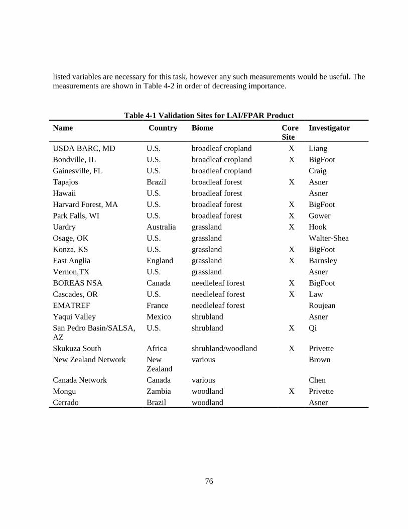
76

listed variables are necessary for this task, however any such measurements would be useful. Themeasurements are shown in Table 4-2 in order of decreasing importance.

Table 4-1 Validation Sites for LAI/FPAR Product

Name Country Biome CoreSite

Investigator

USDA BARC, MD U.S. broadleaf cropland X Liang

Bondville, IL U.S. broadleaf cropland X BigFoot

Gainesville, FL U.S. broadleaf cropland Craig

Tapajos Brazil broadleaf forest X Asner

Hawaii U.S. broadleaf forest Asner

Harvard Forest, MA U.S. broadleaf forest X BigFoot

Park Falls, WI U.S. broadleaf forest X Gower

Uardry Australia grassland X Hook

Osage, OK U.S. grassland Walter-Shea

Konza, KS U.S. grassland X BigFoot

East Anglia England grassland X Barnsley

Vernon,TX U.S. grassland Asner

BOREAS NSA Canada needleleaf forest X BigFoot

Cascades, OR U.S. needleleaf forest X Law

EMATREF France needleleaf forest Roujean

Yaqui Valley Mexico shrubland Asner

San Pedro Basin/SALSA,AZ

U.S. shrubland X Qi

Skukuza South Africa shrubland/woodland X Privette

New Zealand Network NewZealand

various Brown

Canada Network Canada various Chen

Mongu Zambia woodland X Privette

Cerrado Brazil woodland Asner

77

Table 4-2 Land Cover Variables

Land Cover Variable or Characteristic

canopy multispectral reflectance (nadir or bidirectional)

leaf spectra (reflectance and transmittance)

background nadir spectral reflectance (soil + litter)

fraction of areal vegetation cover

vegetation crown allometry (height, width, gap)

phenology (green-up, mature, senescent stage)

vegetation composition (either by species or structural type)

wet or dry status

fraction of non-photosynthesizing vegetation (at min. photosynthetic activity stage)

meteorological data (minimum set)

4.5 Scaling

A pervasive problem for land validation is the scaling of field measurements to the morecoarse resolution of satellite products. Although various schemes will be used, the newly begunBigFoot project will focus directly on EOS scaling issues. The BigFoot approach will includeoverlaying grids of 25 m and 1 km, extending to the 5 km x 5 km “MODIS grid,” at FLUXNETtower sites. BigFoot will initially focus effortsat four EOS Core Sites. Investigators will measureand scale LAI, FPAR, net primary productivity (NPP) and landcover maps to appropriateresolutions for EOS validation. A combined program of field data collection, aircraft overflightsand fine resolution satellite image acquisitions will be used. BigFoot will also attempt tocharacterize and parameterize the -relationship between the measured net ecosystem exchangevalues and the NPP product. This pathfinding activity will test various scaling methodologiesand work with MODLAND to develop a WWW site outlining a recommended strategy.

4.6 Modland QUick Airborne LookS (MQUALS)

To facilitate BigFoot’s and others’ scaling efforts, MODLAND developed the MODLANDQuick Airborne Looks (MQUALS). This program is based on an aircraft remote sensing packagethat includes three digital cameras (red, blue and near-infiared,640x480 pixels), shortwave andnear-infraredalbedometers, a calibrated radiometer with four MODIS spectral bands, and anoptional thermal radiometer. All data are simultaneously collected and stored on a laptopcomputer. A ground-based 4-band radiometer will be used to simultaneously measure irradiance.The complete package was designed to be shipped easily to small aircraftoperators nearvalidation sites for low cost site and reflectance characterization. Initial MQUALS productsshould be available within seven days of data collection. A duplicate MQUALS package willoperate in southern Afiicaas part of SAFARI 2000. Within the greater EOS validation

78

framework, MQUALS will be complimented by remote observations from sensors on NASA’shigh altitude ER-2 and a light aircraft package developed by the CERES team.

4.7 Data Protocols and Dissemination

Successful validation will in part depend on easy access to accurate and documented fielddata. The MODIS Land Team has worked extensively with the Oak Ridge. (ORNL) and EROSData Center DAACs to develop validation data protocols and pathways. Based on distributedWWW mini-archives, the ORNL-based Mercury system will conduct daily data set catalogingand can provide single point access to all EOS validation data (Figure 4-2), The minimal effortrequired to interface with Mercury should allow rapid data submission and public release. Thisevolving data system accommodates a diverse user community in which EOS instrument teams,Validation Investigators, and independent investigators are simultaneously collecting, archiving,distributing and using validation and remote sensing data. Moreover, the ORNL DAAC hasinitiated a vigorous effort to mine historical field data. These data will be used to establishexpected values and reasonable ranges of EOS products in some cases.

EOS land product validation is being planned as part of a long-term implementation plan.Initial validation efforts will both estimate product accuracy and prototype validation schemecomponents. It is hoped the components currently planned, upon successful post-launchevaluation, will be substantially extended to provide more rigorous and comprehensive productevaluation.

79

Figure 4-3 Conceptual design for scaling in the BigFoot project. See URL in Table 4-3

We anticipate that the validation procedures started by the EOS instrument teams andvalidation investigators will act as a catalyst for broader involvement by the research communityin product evaluation. Clear protocols for data collection and WWW archives and access willgive all researchers a simple mechanism for participation. With the recent increase and plannedlaunch of new moderate resolution sensors (e.g., VEGETATION, MODIS AM/PM, GLI, NPP,NPOESS) by different space agencies and the increased availability of higher order standardproducts, the benefits of standard measurement protocols and validation site data sharing areconsiderable. The CEOS Calibration/Validation Working Group is an obvious mechanism toexpand the early developments and lessons learned in EOS land validation into a truly globalvalidation initiative.

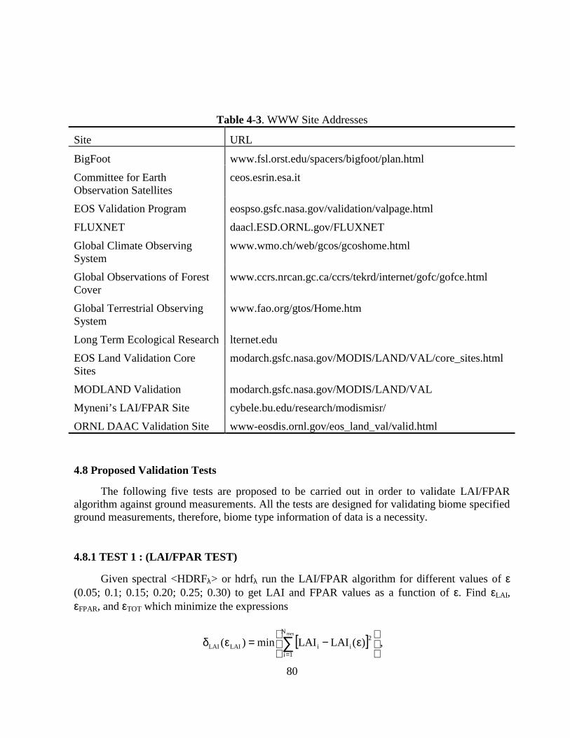
80

Table 4-3. WWW Site Addresses

Site URL

BigFoot www.fsl.orst.edu/spacers/bigfoot/plan.html

Committee for EarthObservation Satellites

ceos.esrin.esa.it

EOS Validation Program eospso.gsfc.nasa.gov/validation/valpage.html

FLUXNET daacl.ESD.ORNL.gov/FLUXNET

Global Climate ObservingSystem

www.wmo.ch/web/gcos/gcoshome.html

Global Observations of ForestCover

www.ccrs.nrcan.gc.ca/ccrs/tekrd/internet/gofc/gofce.html

Global Terrestrial ObservingSystem

www.fao.org/gtos/Home.htm

Long Term Ecological Research lternet.edu

EOS Land Validation CoreSites

modarch.gsfc.nasa.gov/MODIS/LAND/VAL/core_sites.html

MODLAND Validation modarch.gsfc.nasa.gov/MODIS/LAND/VAL

Myneni’s LAI/FPAR Site cybele.bu.edu/research/modismisr/

ORNL DAAC Validation Site www-eosdis.ornl.gov/eos_land_val/valid.html

4.8 Proposed Validation Tests

The following five tests are proposed to be carried out in order to validate LAI/FPARalgorithm against ground measurements. All the tests are designed for validating biome specifiedground measurements, therefore, biome type information of data is a necessity.

4.8.1 TEST 1 : (LAI/FPAR TEST)

Given spectral <HDRFλ> or hdrfλ run the LAI/FPAR algorithm for different values of ε(0.05; 0.1; 0.15; 0.20; 0.25; 0.30) to get LAI and FPAR values as a function of ε. Find εLAI ,εFPAR, and εTOT which minimize the expressions

[ ]

ε−=εδ ∑=

mesN

1i

2iiLAILAI )(LAILAImin)( ,

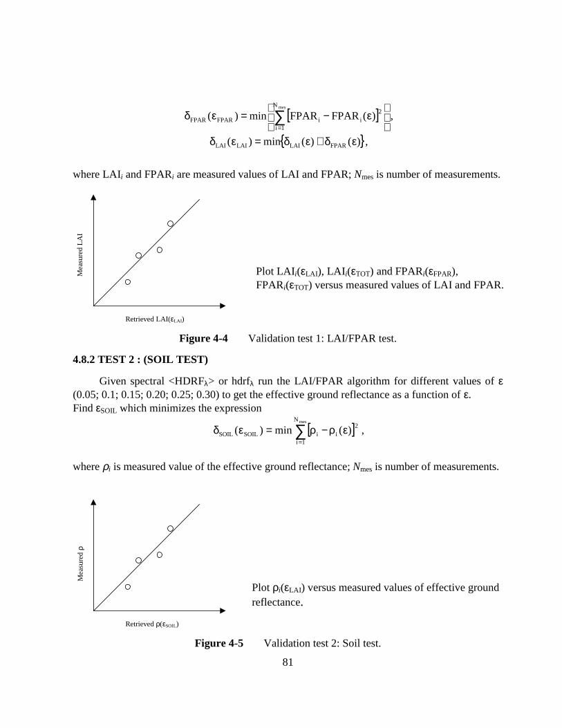
81

[ ]

ε−=εδ ∑=

mesN

1i

2iiFPARFPAR )(FPARFPARmin)( ,

)()(min)( FPARLAILAILAI εδ+εδ=εδ ,

where LAIi and FPARi are measured values of LAI and FPAR; Nmes is number of measurements.

Retrieved LAI(εLAI)

Me

asur

ed

LA

I

Figure 4-4 Validation test 1: LAI/FPAR test.

4.8.2 TEST 2 : (SOIL TEST)

Given spectral <HDRFλ> or hdrfλ run the LAI/FPAR algorithm for different values of ε(0.05; 0.1; 0.15; 0.20; 0.25; 0.30) to get the effective ground reflectance as a function of ε.Find εSOIL which minimizes the expression

[ ]∑=

ερ−ρ=εδmesN

1i

2iiSOILSOIL )(min)( ,

where ρi is measured value of the effective ground reflectance; Nmes is number of measurements.

Retrieved ρ(εSOIL)

Me

asur

ed ρ

Figure 4-5 Validation test 2: Soil test.

Plot LAIi(εLAI ), LAI i(εTOT) and FPARi(εFPAR),FPARi(εTOT) versus measured values of LAI and FPAR.

Plot ρi(εLAI ) versus measured values of effective groundreflectance.

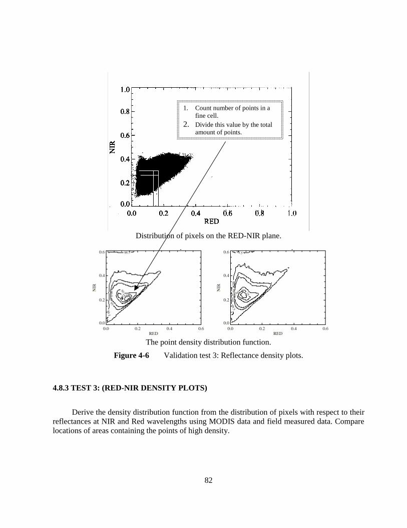
82

Distribution of pixels on the RED-NIR plane.

The point density distribution function.

Figure 4-6 Validation test 3: Reflectance density plots.

4.8.3 TEST 3: (RED-NIR DENSITY PLOTS)

Derive the density distribution function from the distribution of pixels with respect to theirreflectances at NIR and Red wavelengths using MODIS data and field measured data. Comparelocations of areas containing the points of high density.

1. Count number of points in afine cell.

2. Divide this value by the totalamount of points.

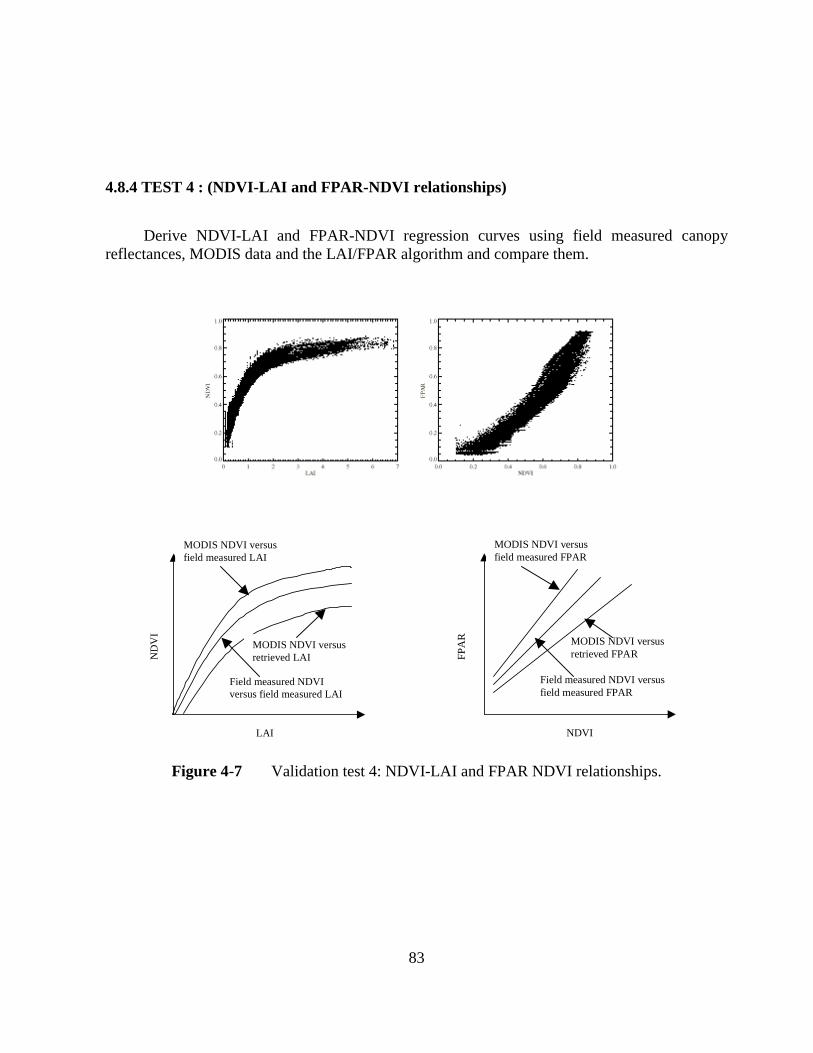
83

4.8.4 TEST 4 : (NDVI-LAI and FPAR-NDVI relationships)

Derive NDVI-LAI and FPAR-NDVI regression curves using field measured canopyreflectances, MODIS data and the LAI/FPAR algorithm and compare them.

LAI

ND

VI

MODIS NDVI versusfield measured LAI

Field measured NDVIversus field measured LAI

MODIS NDVI versusretrieved LAI

NDVI

FP

AR

MODIS NDVI versusfield measured FPAR

Field measured NDVI versusfield measured FPAR

MODIS NDVI versusretrieved FPAR

Figure 4-7 Validation test 4: NDVI-LAI and FPAR NDVI relationships.

84

4.8.5 TEST 5 : (INFORMATION CONVEYED ABOUT LAI BY HDRF)

Steps:1. Find LAI distribution function using all available values of measured LAI.

LAI

Pro

bab

ility p1

p2

p5

Figure 4-8 Validation test 5: LAI distribution function.

2. Evaluate the entropy: ∑=

−=LAIN

1kkk0 plogpE .

3. Evaluate the conditional LAI probability function F(lai|M), where M is the set of spectralcanopy reflectances.

hdrfred

hdrf n

ir

M

lai

Pro

bab

ility q1

q2

q3

Figure 4-9 Validation test 5: LAI probability function.

Example of the evaluation of the conditional probability function using canopy reflectances atRed and NIR wavelength.

4. Evaluate the joint LAI-lai(M) probability function, i.e.,

1pLAIN

1kk =∑

=

NLAI is number of measurements

1)M(qMN

1kk =∑

=

85

)LAI)M(lai and LAIob(LAIPr)M(p jij,i === .

5. Evaluate the "information conveyed about LAI by HDRF" as:

∑∑= =

+=LAI MN

1i

N

1j j

j,ij,i0 )M(q

)M(plogpE)M(E .

6. Do the same for retrieved values of LAI.7. Compare results.

M

E(M

)

E(M) obtained from measurements E(M) obtained from the algorithm

Figure 4-10 Validation test 5: Information convey curves.

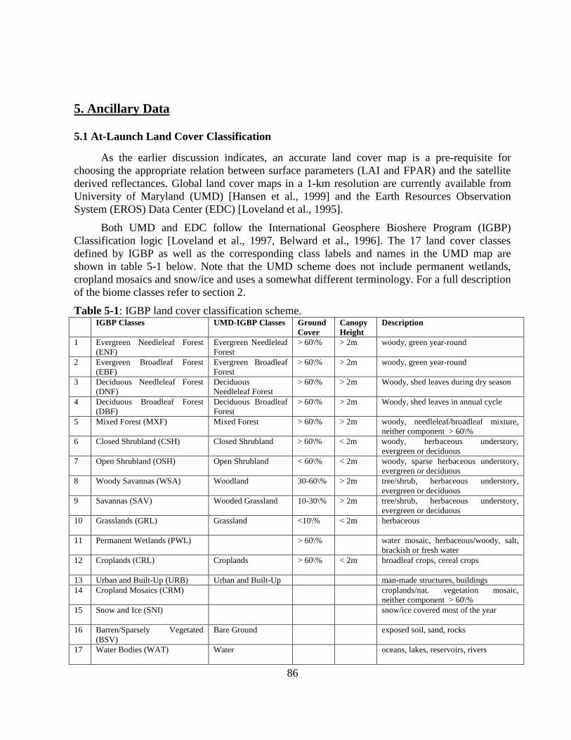
86

5. Ancillary Data

5.1 At-Launch Land Cover Classification

As the earlier discussion indicates, an accurate land cover map is a pre-requisite forchoosing the appropriate relation between surface parameters (LAI and FPAR) and the satellitederived reflectances. Global land cover maps in a 1-km resolution are currently available fromUniversity of Maryland (UMD) [Hansen et al., 1999] and the Earth Resources ObservationSystem (EROS) Data Center (EDC) [Loveland et al., 1995].

Both UMD and EDC follow the International Geosphere Bioshere Program (IGBP)Classification logic [Loveland et al., 1997, Belward et al., 1996]. The 17 land cover classesdefined by IGBP as well as the corresponding class labels and names in the UMD map areshown in table 5-1 below. Note that the UMD scheme does not include permanent wetlands,cropland mosaics and snow/ice and uses a somewhat different terminology. For a full descriptionof the biome classes refer to section 2.

Table 5-1: IGBP land cover classification scheme.IGBP Classes UMD-IGBP Classes Ground

CoverCanopyHeight

Description

1 Evergreen Needleleaf Forest(ENF)

Evergreen NeedleleafForest

> 60\% > 2m woody, green year-round

2 Evergreen Broadleaf Forest(EBF)

Evergreen BroadleafForest

> 60\% > 2m woody, green year-round

3 Deciduous Needleleaf Forest(DNF)

DeciduousNeedleleaf Forest

> 60\% > 2m Woody, shed leaves during dry season

4 Deciduous Broadleaf Forest(DBF)

Deciduous BroadleafForest

> 60\% > 2m Woody, shed leaves in annual cycle

5 Mixed Forest (MXF) Mixed Forest > 60\% > 2m woody, needleleaf/broadleaf mixture,neither component > 60\%

6 Closed Shrubland (CSH) Closed Shrubland > 60\% < 2m woody, herbaceous understory,evergreen or deciduous

7 Open Shrubland (OSH) Open Shrubland < 60\% < 2m woody, sparse herbaceous understory,evergreen or deciduous

8 Woody Savannas (WSA) Woodland 30-60\% > 2m tree/shrub, herbaceous understory,evergreen or deciduous

9 Savannas (SAV) Wooded Grassland 10-30\% > 2m tree/shrub, herbaceous understory,evergreen or deciduous

10 Grasslands (GRL) Grassland <10\% < 2m herbaceous

11 Permanent Wetlands (PWL) > 60\% water mosaic, herbaceous/woody, salt,brackish or fresh water

12 Croplands (CRL) Croplands > 60\% < 2m broadleaf crops, cereal crops

13 Urban and Built-Up (URB) Urban and Built-Up man-made structures, buildings14 Cropland Mosaics (CRM) croplands/nat. vegetation mosaic,

neither component > 60\%15 Snow and Ice (SNI) snow/ice covered most of the year

16 Barren/Sparsely Vegetated(BSV)

Bare Ground exposed soil, sand, rocks

17 Water Bodies (WAT) Water oceans, lakes, reservoirs, rivers

87

Figure 5-1: IGBP land cover classes for North America in the EDC and UMD maps that cannotbe directly translated into biome classes.

88

Figure 5-2: Cereal crops, broadleaf crops, and cropland mosaics mapped from the NorthAmerica EDC SLCR map.

Unfortunately, the translation of IGBP classes into the classes in the biome schemerequired for the MODIS/MISR LAI/FPAR algorithm is ambiguous with respect several classes.In particular, direct translation of the 17 IGBP classes into the six biome classes is not possiblefor the IGBP classes 5, 6, 8, 12, 14 (mixed forest, closed shrublands, woody savannas, croplandsand croplands mosaic, respectively). Aggregation of the IGBP maps into the biome schemetherefore introduces distortions of the land cover proportions and may cause classification errorsthat are relatively severe from the viewpoint of radiative transfer modeling.

To illustrate the magnitude of distortion introduced by simple aggregation, mixed forests,closed shrublands and woody savannas were mapped from the UMD and EDC maps (Figure 5-1). The map comparison shows significant differences in both extent and spatial distribution ofmixed forests, closed shrublands and woody savannas. Table 5-2 shows the areal extent of theseclasses in the EDC and UMD maps. Furthermore, the IGBP classification scheme does notdistinguish between broadleaf crops and cereal crops. From the viewpoint of radiative transfer,however, this distinction is very important. A disaggregation of croplands and cropland mosaics(IGBP class 11 and 14) into cereal crops (biome 1) and broadleaf crops (biome 3) is not possible.

89

Using a simple aggregation scheme, e.g. assigning all croplands to biome 1, major areas wouldbe spuriously assigned to one biome class (Figure 5-2 and Table 5-2).

The only digital map source at global scales providing more detailed information on thedistribution of land cover is the Global Land Cover Characterization Data Base (GLCC)available from EDC [Loveland et al. 1995]. This data set is derived from 1-km Advanced VeryHigh Resolution Radiometer (AVHRR) data spanning a 12-month period (April 1992- March1993) and is based on a flexible data base structure and seasonal land cover regions concepts.Seasonal land cover regions (SLCR) provide a framework for presenting the temporal and spatialpattern of vegetation. The regions are composed of relatively homogeneous land coverassociations, which exhibit distinctive phenology (i.e., onset, peak, and seasonal duration ofgreenness). A time series of 12-month NDVI composites was used in an unsupervised clusteringalgorithm. The resulting clusters were then labeled using extensive post-classificationstratification and refinement techniques. The UMD map, on the other hand, was generated with asupervised classification approach using decision trees [Hansen et al. 1999]. Also, post-classification was an important methodological step to remove major misclassifications in theUMD map.

Table 5-2: A: Areal extent of mixed forests, closed shrublands, woody savannas and croplandsin the EDC and UMD map. B: Areal Extent of broadleaf crops, cereal crops and croplandmosaics in the SLCR map (both North America).A EDC UMD

Mixed Forests 2,854,132 km2 1,349,244 km2

Closed Shrublands 579,582 km2 1,703,853 km2

Woody Savannas 1,658,740 km2 3,113,640 km2

Croplands 1,852,240 km2 1,781,694 km2

B SLCRBroadleaf Crops 1,055,278 km2

Cereal Crops 1,487,628 km2

Cropland Mosaic 544,887 km2

The GLCC project defined 205 SCLR for North America, 255 for Eurasia, 167 for South-America, 197 for Africa and 137 for Australia-Pacific. The narrow definition of the SLCRclasses allows their aggregation into broader classes of other desired classification schemes, e.g.,the 6-biome scheme. Look up tables (LUT) for the aggregation of SLCR classes into variousexisting classification schemes as well as ancillary data sheets, were provided by EDC and usedas a guideline for the translation to 6 biomes performed for the at-launch MODIS/MISRLAI/FPAR land cover data set.

To generate a map in the 6-biome scheme for the MODIS/MISR LAI/FPAR algorithm, themap from UMD was used in association with the SLCR map. More specifically, for those classes

90

in the UMD-IGBP scheme that can be directly translated into one of the biome classes, a directclass assignment was performed. This applies to evergreen needleleaf forests, evergreenbroadleaf forests, deciduous needleleaf forests, deciduous broadleaf forests, wooded grassland,open shrubland, grasslands, bare ground, and urban/built-up. For classes, that do not allow adirect translation, the respective SLCR label was retrieved and a biome class label was assignedusing the IGBP-biome LUT described above. This routine was performed on a per-pixel basis.

Figure 5-3: At-launch global biome map derived from the UMD land cover map and the EDCSLCR map.

The use of the SLCR maps in conjunction with the ancillary information in the global landcover characterization data base allows to resolve ambiguities in translating the UMD map intothe 6-biome scheme. The SLCR labels were particularly useful for disaggregating the croplandclass into broadleaf crops and cereal crops. The ancillary information about structural propertiesof the land cover types in the GLCC database also helped disaggregating the closed shrublandand woody savannas classes. In the case of mixed forests the disaggregation into either

91

needleleaf forests of broadleaf forests remained ambiguous in many cases, since many areas arein fact characterized by a mixture of both forest types. Using the LUT for each of the fivecontinents, a pixel labeled according to the biome scheme can be related to its original class labelin the UMD land cover map. This allows comparisons of various MODIS products (e.g. netprimary productivity or leaf area index) that used modified versions of the UMD map in theiralgorithm.

92

5.2 Look-Up Table Structure

Summary of parameters determining the size of the LUT

Parameter Value Description of Content

Maxbands 7 Number of MODIS spectral bands for whichthe LUT was created.

Nbiome 6 Number of biome types.

Specdim 152 Number of points at which the spectral leafalbedo is given.

Maxviewpol 5 Number of sensor zenith intervals for whichthe LUT was created.

Maxviewazi 6 Number of sensor azimuth intervals forwhich the LUT was created

Maxsunpol 4 Number of solar zenith intervals for whichthe LUT was created

Laidim 40 Number of LAI values for which the LUTwas created

Maxsat 41 Number of saturation curve points for whichthe LUT was created

Maxsoildim 29 Number of patterns of spectral effectiveground reflection defined at the MODISspectral bands which the LUT was created

Maxpixel 1000 Maximum pixels for run. This parameterdoes not effect the LUT size.

The size of the LUT can be reduced by setting laidim=29 (instead of 40). However it does noteffect the program execution time. Therefore I recommend to take laidim=40. It will giveus a possibility to influence the algorithm by varying laidimbio and laimax inBu_anc_soil.txt.

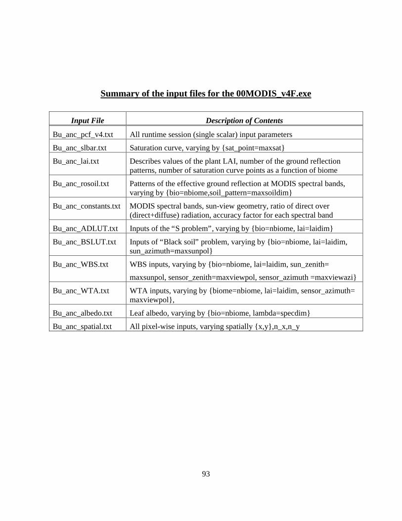
93

Summary of the input files for the 00MODIS_v4F.exe

Input File Description of Contents

Bu_anc_pcf_v4.txt All runtime session (single scalar) input parameters

Bu_anc_slbar.txt Saturation curve, varying by sat_point=maxsat

Bu_anc_lai.txt Describes values of the plant LAI, number of the ground reflectionpatterns, number of saturation curve points as a function of biome

Bu_anc_rosoil.txt Patterns of the effective ground reflection at MODIS spectral bands,varying by bio=nbiome,soil_pattern=maxsoildim

Bu_anc_constants.txt MODIS spectral bands, sun-view geometry, ratio of direct over(direct+diffuse) radiation, accuracy factor for each spectral band

Bu_anc_ADLUT.txt Inputs of the “S problem”, varying by bio=nbiome, lai=laidim

Bu_anc_BSLUT.txt Inputs of “Black soil” problem, varying by bio=nbiome, lai=laidim,sun_azimuth=maxsunpol

Bu_anc_WBS.txt WBS inputs, varying by bio=nbiome, lai=laidim, sun_zenith=

maxsunpol, sensor_zenith=maxviewpol, sensor_azimuth =maxviewazi

Bu_anc_WTA.txt WTA inputs, varying by biome=nbiome, lai=laidim, sensor_azimuth=maxviewpol,

Bu_anc_albedo.txt Leaf albedo, varying by bio=nbiome, lambda=specdim

Bu_anc_spatial.txt All pixel-wise inputs, varying spatially x,y,n_x,n_y

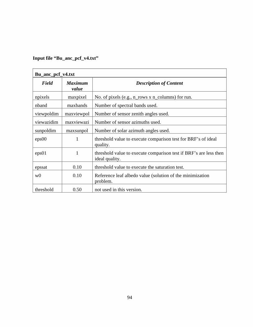
94

Input file “Bu_anc_pcf_v4.txt”

Bu_anc_pcf_v4.txt

Field Maximumvalue

Description of Content

npixels maxpixel No. of pixels (e.g., n_rows x n_columns) for run.

nband maxbands Number of spectral bands used.

viewpoldim maxviewpol Number of sensor zenith angles used.

viewazidim maxviewazi Number of sensor azimuths used.

sunpoldim maxsunpol Number of solar azimuth angles used.

eps00 1 threshold value to execute comparison test for BRF’s of idealquality.

eps01 1 threshold value to execute comparison test if BRF’s are less thenideal quality.

epssat 0.10 threshold value to execute the saturation test.

w0 0.10 Reference leaf albedo value (solution of the minimizationproblem.

threshold 0.50 not used in this version.

95

Input file “Bu_anc_slbar.txt”

Definition. The parametric plot maxmax*

minmin** ,)(),( LgLLgLdLL ⋅≤≤⋅ , is defined to

be a saturation curve. Here

∫∫ Φ−=Φ=max

min

max

min

),()]([)(,),()( *2****LAI

LAI

LAI

LAI

lLdLLlLdlLdlLL ,

and gmin, gmax, Lmin and Lmax are introduced in Section 2.9.

Bu_anc_slbar.txt

Field Value Range Description of Contents

isat 1,2,…,maxsat Number of the arameter L*

satwlai for biome 1 5,…,10 Value of )( *LL for biome 1

satdwlai for biome 1 0…10 Value of )( *Ld for biome 1

satwlai for biome 2 5,…,10 Value of )( *LL for biome 2

satdwlai for biome 2 0…10 Value of )( *Ld for biome 2

satwlai for biome 3 5,…,10 Value of )( *LL for biome 3

satdwlai for biome 3 0…10 Value of )( *Ld for biome 3

satwlai for biome 4 5,…,10 Value of )( *LL for biome 4

satdwlai for biome 4 0…10 Value of )( *Ld for biome 4

satwlai for biome 5 5,…,10 Value of )( *LL for biome 5

satdwlai for biome 5 0…10 Value of )( *Ld for biome 5

satwlai for biome 6 5,…,10 Value of )( *LL for biome 6

satdwlai for biome 6 0…10 Value of )( *Ld for biome 6

96

Input file “Bu_ans_lai.txt”

Bu_anc_soil.txt

Field Value Range Description of Contents

Biome 1,…,nbiome Biome land cover class code

Soildimbio ≤ maxsoildim Number of patterns for the effective ground reflectancesSection 2.2, Eq. (2) at MODIS spectral bands

Laidimbio ≤ laidim Number of LAI values LAI (Sect. 2.2).

nsat ≤ Maxsat Number of saturation curve points

Biome1 Between 0.1 and 9.85 Lai values for biome 1

Biome2 Between 0.1 and 9.85 Lai values for biome 2

Biome3 Between 0.1 and 9.85 Lai values for biome 3

Biome4 Between 0.1 and 9.85 Lai values for biome 4

Biome5 Between 0.1 and 9.85 Lai values for biome 5

Biome6 Between 0.1 and 9.85 Lai values for biome 6

Input file “Bu_ans_rosoil.txt”

This file contains the effective ground reflection defined by Section 2.2, Eq. (2) at the MODISspectral bands.

Bu_anc_rosoil.txt

Field Value Range Description of Contents

Biome 1,…,nbiome Biome land cover class code

Pattern 1,…, maxsoildim Soil pattern number

Band 1 between 0 and 1 The effective ground reflection at the 1st MODIS band.

Band 2 between 0 and 1 The effective ground reflection at the 2nd MODIS band.

Band 3 between 0 and 1 The effective ground reflection at the 3rd MODIS band.

Band 4 between 0 and 1 The effective ground reflection at the 4th MODIS band.

Band 5 between 0 and 1 The effective ground reflection at the 5th MODIS band.

Band 6 between 0 and 1 The effective ground reflection at the 6th MODIS band.

Band 7 between 0 and 1 The effective ground reflection at the 7th MODIS band.

97

Input file “Bu_anc_constants.txt”

Bu_anc_constants.txt

Field Value Range Description of Contents

lam 645, 859, 469, 555, 1240, 1640, 2130 MODIS spectral bands used byalgorithm; lam=1,2,…,nbands

bio, wMODIS 1 7 values between 0 and 1 Biome #, values of leaf albedo atthe MODIS spectral band.

bio, wMODIS 2 7 values between 0 and 1 Biome #, values of leaf albedo atthe MODIS spectral band.

bio, wMODIS 3 7 values between 0 and 1 Biome #, values of leaf albedo atthe MODIS spectral band.

bio, wMODIS 4 7 values between 0 and 1 Biome #, values of leaf albedo atthe MODIS spectral band.

bio, wMODIS 5 7 values between 0 and 1 Biome #, values of leaf albedo atthe MODIS spectral band

bio, wMODIS 6 7 values between 0 and 1 Biome #, values of leaf albedo atthe MODIS spectral band

fdir0 7 values between 0 and 1 Ratio of direct over radiation foreach band

epl 7 value between 0 and 1 Uncertainty factor for each band

viewpol 8.5, 22.5, 37.5, 52.5, 67.5 Sensor zenith angles. Number ofangles modeled is maxviewpol.

viewazi 25., 55., 85., 115., 145., 180. Sensor azimuths. Number ofangles modeled is maxviewazi

sunpol 22.5, 37.5, 52.5, 70. Solar zenith angles. Number ofangles modeled is maxsunpol.

See routine "Prep_angles_v4.f" for detailed description of Sun-sensor geometry.

98

Input file “Bu_anc_ADLUT.txt”

Bu_anc_ADLUT.txt

Field Value Description of Contents

Biome 1,2,3,4,5,6 Biome land cover class code

LAI values 1,2,3…laidim Number of LAI values is laidim.

pAAD 0.0< pAAD<1 Solution of the minimization problem Knyazikhin et al. 1998b, Eq. (49) for the “Sproblem.”

pABS 0.0< pABS<1 Solution of the minimization problem Knyazikhin et al. 1998b, Eq. (49) for the “Blacksoil problem.”

AAD 0.0< AAD<1 Fraction of absorbed PAR by vegetation at thereference leaf albedo w0 for the “S problem.” Thisis value q

iso 0,λa introduced on the right side of

Section 2.5, Eq. (29).

pTAD 0.0< pTAD<1 Solution ptiso of the minimization problem Knyazikhin et al. 1998b, Eq. (50) for the “Sproblem.”

TAD 0.0< TAD<1 Canopy transmittance at the reference leaf albedow0 for the “S problem.” This is value qiso 0,λt

introduced on the right side of Section 2.5, Eq.(25).

99

Input File “Bu_anc_BSLUT.txt”

Bu_anc_BSLUT.txt

Field Value Description of Contents

Biome 1,2,3,4,5,6 Biome land cover class code

LAI values 1,2,3…laidim Number of LAI values is laidim.

sunpol 22.5, 37.5, 52.5, 70. Solar zenith angles. Number of angles modeled is maxsunpol.

pTBSdir 0.0< pTBSdir<1 Solution of the minimization problem Knyazikhin et al.1998b, Eq. (50) for the “Black soil problem.” Radiation fieldis generated by direct component of incoming solar radiation.

pTBSdif 0.0< pTBSdif<1 Solution of the minimization problem Knyazikhin et al.1998b, Eq. (50) for the “Black soil problem.” Radiation fieldis generated by diffuse component of incoming solarradiation.

ABSDIR 0.0< ABSDIR<1 Fraction of absorbed PAR by vegetation at the reference leafalbedo w0 for the “Black soil” problem. Radiation field isgenerated by direct component of incoming solar radiation.

ABSDIF 0.0< ABSDIF<1 Fraction of absorbed PAR by vegetation at the reference leafalbedo w0 for the “Black soil” problem. Radiation field isgenerated by diffuse component of incoming solar radiation.

TBSDIR 0.0< TBSDIR<1 Canopy transmittance at the reference leaf albedo w0 for the“Black soil” problem. Radiation field is generated by directcomponent of incoming solar radiation.

TBSDIF 0.0< TBSDIF<1 Canopy transmittance at the reference leaf albedo w0 for the“Black soil” problem. Radiation field is generated by diffusecomponent of incoming solar radiation.

The variables ABSDIR, ABSDIF, TBSDIF and TBSDIF form the values hembs 0,λa introduced by

Section 2.5, Eq. (29) and qhembs

,, 0λt introduced by Section 2.5, Eq. (27) at the reference

leaf albedo ω0=ω(λ0) as

ABSDIF*fdir)(1ABSDIR*fdir0, −+=hem

bs λa ,

TBSDIF*fdir)(1TBSDIR*fdir0, −+=hem

bs λt .

100

Input file “Bu_anc_WBS.txt”

This input file contains coefficient π⋅wbs,λ at the MODIS spectral bands. Here wbs,λ is the weightdefined by Section2.7, Eq. (50).

Bu_anc_WBS.txt

Field Value Description of Contents

BiomeClass 1,2,3,4,5,6 Biome class code

LAI values 1,2,3…laidim Number of LAI values modeled is laidim.

sunpol 22.5, 37.5, 52.5, 70. Solar zenith angles. Number of anglesmodeled is maxsunpol.

viewpol 8.5, 22.5, 37.5, 52.5, 67.5 Sensor zenith angles. Number of anglesmodeled is maxviewpol.

viewazi 25., 55., 85., 115., 145., 180. Sensor azimuths. Number of anglesmodeled is maxviewazi

Band1 between 0 and 10 Value of π⋅wbs,λ at the 1st MODIS band.

Band2 between 0 and 10 Value of π⋅wbs,λ at the 2nd MODIS band.

Band3 between 0 and 10 Value of π⋅wbs,λ at the 3rd MODIS band.

Band4 between 0 and 10 Value of π⋅wbs,λ at the 4th MODIS band.

Band5 between 0 and 10 Value of π⋅wbs,λ at the 5th MODIS band.

Band6 between 0 and 10 Value of π⋅wbs,λ at the 6th MODIS band.

Band7 between 0 and 10 Value of π⋅wbs,λ at the 7th MODIS band.

101

Input file “Bu_anc_WTA.txt”

This input file contains coefficient qwλπ ⋅ at the MODIS spectral bands. Here qwλ is the weight

defined by Section2.7, Eq. (51).

Bu_anc_WTA.txt

Field Value Description of Contents

BiomeClass 1,2,3,4,5,6 Biome class code

LAI values 1,2,3…laidim Number of LAI values modeled is laidim.

viewpol 8.5, 22.5, 37.5, 52.5, 67.5 Sensor zenith angles. Number of anglesmodeled is maxviewpol.

Band1 between 0 and 10 Value of qwλπ ⋅ at the 1st MODIS band.

Band2 between 0 and 10 Value of qwλπ ⋅ at the 2nd MODIS band.

Band3 between 0 and 10 Value of qwλπ ⋅ at the 3rd MODIS band.

Band4 between 0 and 10 Value of qwλπ ⋅ at the 4th MODIS band.

Band5 between 0 and 10 Value of qwλπ ⋅ at the 5th MODIS band.

Band6 between 0 and 10 Value of qwλπ ⋅ at the 6th MODIS band.

Band7 between 0 and 10 Value of qwλπ ⋅ at the 7th MODIS band.

102

Input file “Bu_anc_spatial.txt”

This table contains one record per pixel, mirroring the spatially defined (e.g. 2D) inputs of theMODIS production algorithm.

Bu_anc_spatial.txt

Field Value Description of Contents

Biome 1,2,3,4,5,6 Biome, land cover class code

qA 00; 01; 02; 03 00 ideal quality of BRF; 01 less then ideal; 02and 03 BRF is not produced

sen_azi 0.0 <= sen_aazi < 360.0 Sensor azimuth at this pixel

sen_pol 0.0 <= sen_pol < 90.0 Sensor zenith at this pixel

sol_azi 0.0 <= sol_azi < 360.0 Solar azimuth at this pixel

sol_pol 0.0 <= sol_pol < 90.0 Solar zenith at this pixel

Band1 0 < b1 < 100 BRF at the 1st MODIS band

Band2 0 < b2 < 100 BRF at the 2nd MODIS band

Band3 0 < b3 < 100 BRF at the 3rd MODIS band

Band4 0 < b4 < 100 BRF at the 4th MODIS band

Band5 0 < b5 < 100 BRF at the 5th MODIS band

Band6 0 < b6 < 100 BRF at the 6th MODIS band

Band7 0 < b7 < 100 BRF at the 7th MODIS band

103

Input file “Bu_anc_albedo.txt”

This input file contains the spectral leaf albedo varying by biome. The definition of thisparameter is given by Section2.6, Eq. (45). See also Section 2.4.5, Fig. 2-2

Bu_anc_albedo.txt

Field Value Description of Contents

Biome 1,2,3,4,5,6 Biome land cover class code

Lambda 400 ≤ λ ≤ 702 Wavelength (nm). Number of spectral points isspecdim.

Leaf albedo 0 < ω(λ) ≤ 1 Leaf albedo at this wavelength

Output file “Bu_output.txt”

Bu_anc_output.txt

Field Value Description of Contents

FPAR 0 ≤ f ≤ 1 FPAR, fraction of photosynthetically active radiationabsorbed by vegetation.

QAFPAR 0 ≤ q ≤ 1 Variance of FPAR

LAI 0 < lai < 10 LAI value

QALAI 0 < q < 1 Variance of LAI

qA 0,1,2,3 0 - algorithm was executed: 1 - algorithm was executed.Saturation; 2 – Algorithm was not executed becauseBRF's were not available (cloud or "or other reasons");or algorithm was not executed because view or sunzenith was too law; 3: algorithm fails.

104

6. Programming and Procedural Considerations

The MODIS land FPAR, LAI Level 3 algorithms were developed jointly by personnel atBoston University and the University of Montana SCF. The Boston University team developedthe radiative-transfer (R-T) derivative science core logic and the R-T driven lookup tablescomprising the core science, the direct-retrieval lookup tables, and prototype software forexercising the core logic. The University of Montana SCF team is responsible for developing,testing, and maintaining the EOSDIS Core System (ECS) production version of the software.QA tasks are shared between the two institutions, with the MOD15A1 QA activities conducted atBoston University, and the MOD15A2 QA activities run at University of Montana SCF.

The FPAR, LAI software codes are collectively organized into two software components:

• a daily executable (MOD_PR15A1, as PGE-33), used to produce a series of candidate dailyproducts, and

• an 8-day executable (MOD_PR15A2, as PGE-34), used to produce the 8-day compositeFPAR,LAI product archived at the Eros Data Center DAAC.

Each of these components defines a registered NASA EOSDIS Earth Science Data Type(EDST), providing users with a consistent product metadata organization supported by variousend-user browse and data order environments. The daily product produced by MOD_PR15A1generates the MOD15A1 ESDT, and the 8-day product generated by MOD_PR15A2 generatesthe archive MOD15A2 ESDT. Note that the daily product is used exclusively by thecompositing process, and is not archived by the DAAC over time.

6.1 Programming Issues

6.1.1 Implementation Software Environment

The MOD15A1 and MOD15A2 FPAR, LAI software codes are written to comply with anumber of standards, and to interoperate with several supporting binary libraries. The codes arewritten in ANSI C and are POSIX 1.x compliant. Both daily and 8-day codes link to themandatory NASA Software Data Production Toolkit library (SDPTK v.5.2.4), the NASA HDF-EOS library v.2.4), and our SCF API -- the MODIS-University of Montana (MUM) API v. 2.2 .The table below breaks down the lines-of-code for our at-launch FPAR,LAI algorithms:

105

FPAR, LAI At-launch Lines-of-code (LOC) MetricsCode Layer Lines Of Code Percent of CodeMOD15A1 (PGE33) 13,336 28 %MUM library 33,588 72 %PGE-33 subtotal: 46,924 -MOD15A2 (PGE34) 7275 18 %MUM library 33,588 82 %PGE-34 subtotal: 40,863 -Total, All Codes 54199 -

6.1.2 Software Design

In designing our at-launch algorithms, emphasis was placed on code robustness, reliabilityand maintainability. A significant fraction of the ECS production code developed at theMontana SCF rests on the common MUM API foundations. Larger amounts of code re-usegenerally promote life-cycle reliability in several ways: a) the total number of potential points-of-failure (system-wide) are reduced across all algorithms sharing a common foundation, and b)the life-cycle maintenance effort required to support the shared foundation (API) code is spentjust once while each "client" benefits from the software services it provides.

Another common design thread running throughout our implementations is the emphasison data-driven parameterization of the algorithm software. By "data driven" we refer to theexternalization of key software inputs, to allow some revisions in program behavior withouthaving to recompile and link the software. The lookup table (LUT) orientation of MOD15A1 isthe best example of this type of externalization, stored in the static ancillary HDFEOS(MOD15_ANC_v21.hdf) file available to the algorithm at runtime. We also store all thedefining characteristics of all ESDT product gridfields in this ancillary file, allowing minor filespecification changes to be effected from outside the software.

The following diagram illustrates the high level organization (schema) used in MOD15A1;an almost identical schema is used for MOD15A2:

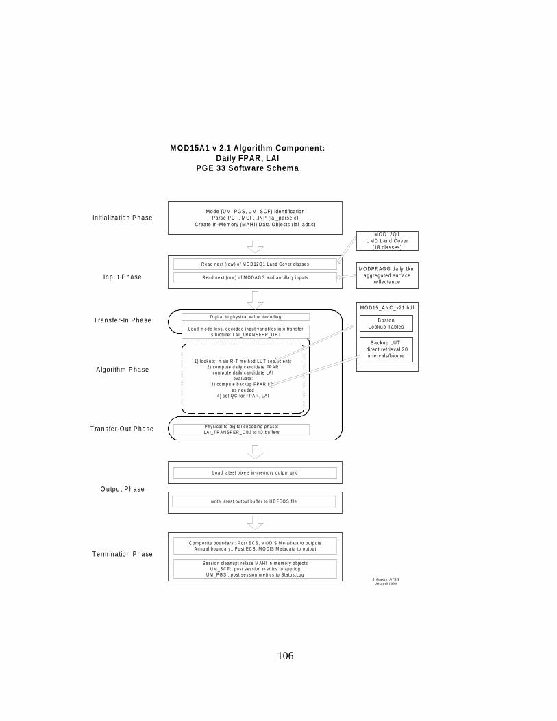
106

MOD15A1 v 2.1 Algorithm Com ponent:Daily FPAR, LAI

PGE 33 Softw are Schem a

Inpu t P hase

In itia liza tion P hase

T ransfe r-In P hase

A lgo rithm P hase

T ransfe r-O u t P hase

O utpu t P hase

T erm ina tion P hase

M ode U M _PG S, U M _SC F Iden tifica tionParse PC F, M CF , .IN P (la i_parse.c )

C rea te In -M em ory (M AH I) D a ta O b jects (la i_adt.c)

1 ) looku p :: m a in R -T m e th od L U T co e ffic ien ts2 ) co m pu te d a ily ca nd ida te F P A R

com p ute da ily can d id a te LA Ieva lua te :

3 ) co m pu te b acku p F P A R ,L A Ias ne ed ed

4) se t Q C fo r F P A R , L A I

P h ys ica l to d ig ita l en cod in g ph ase :LA I_ T R A N S F E R _ O B J to IO bu ffe rs

C om p os ite bou nd ary :: P os t E C S , M O D IS M etad a ta to o u tpu tsA n nu a l b ou nd ary :: P o s t E C S , M O D IS M e ta da ta to o u tpu t

S e ss io n cle an up : re lase M A H I in -m e m ory o b jec tsU M _S C F :: po s t sess ion m e tr ics to ap p .lo g

U M _P G S :: pos t se ssio n m e trics to S ta tus .Lo g

R ea d ne x t (row ) o f M O D 12 Q 1 L an d C o ver c la sse s

R ea d ne x t (row ) o f M O D A G G a nd a nc illa ry in pu ts

D ig ita l to p hys ica l va lue d ecod ing

Lo ad m o de -le ss , de co de d inp u t va ria b les in to tran s fe rs truc tu re : L A I_T R A N S F E R _O B J

Lo ad la te s t p ixe ls in -m em o ry ou tp u t g rid

J. G lassy, NTSG26 April 1999

M O DPR AG G daily 1kmaggrega ted surface

reflectance

M O D12Q 1U M D Land Cover

(18 c lasses)

M O D15_AN C_v21 .hd f

BostonLookup Tab les

Backup LU T: d irect retrieva l 20

in te rvals /b iom e

w rite la tes t o u tpu t bu ffe r to H D F E O S file

107

6.1.3 Spatial Projection

The MOD15A1 and MOD15A2 algorithms, like most MODIS Land processes, areorganized to accept global coverage inputs, and produce global coverages either daily (PGE-33)or on an 8-day (PGE-34) timestep. Rather than process synoptic 1 KM spatial resolution images,the MODIS Land team has adopted a contiguous land tile scheme, based on the IntegerizedSinusoidal Grid -- a map projection derived from the sinusoidal map projection (with the GeneralCartographic Map Projection code of GCTP_ISINUS). This projection defines a total of 648tiles globally, at 10 degree resolution. We currently estimate that 289 tiles of 648 will beclassified as "land" tiles, and thus represent the maximum spatial extent our global algorithmswill process. Refer to http://modland.nascom.nasa.gov/developers/bndrytb2.html for additionaldetails. The figure below graphically depicts the IS grid (assuming the standard 10 degreesprocessing tiles) we expect to work with at-launch. Each individual tiles in this grid includesapproximately 1200 x 1200 1 km pixels:

6.1.4 Data Flows and Dependencies

The MOD15A1 (fired daily) and MOD15A2 (fired once each 8-day period) executablesare positioned towards the end of the Land L4/L4 processing chain. Our algorithms are thereforequite dependent on the quality and correct functioning of all upstream processes. The followingdiagram illustrates the input I/O dependencies for MOD15A1 and MOD15A2:

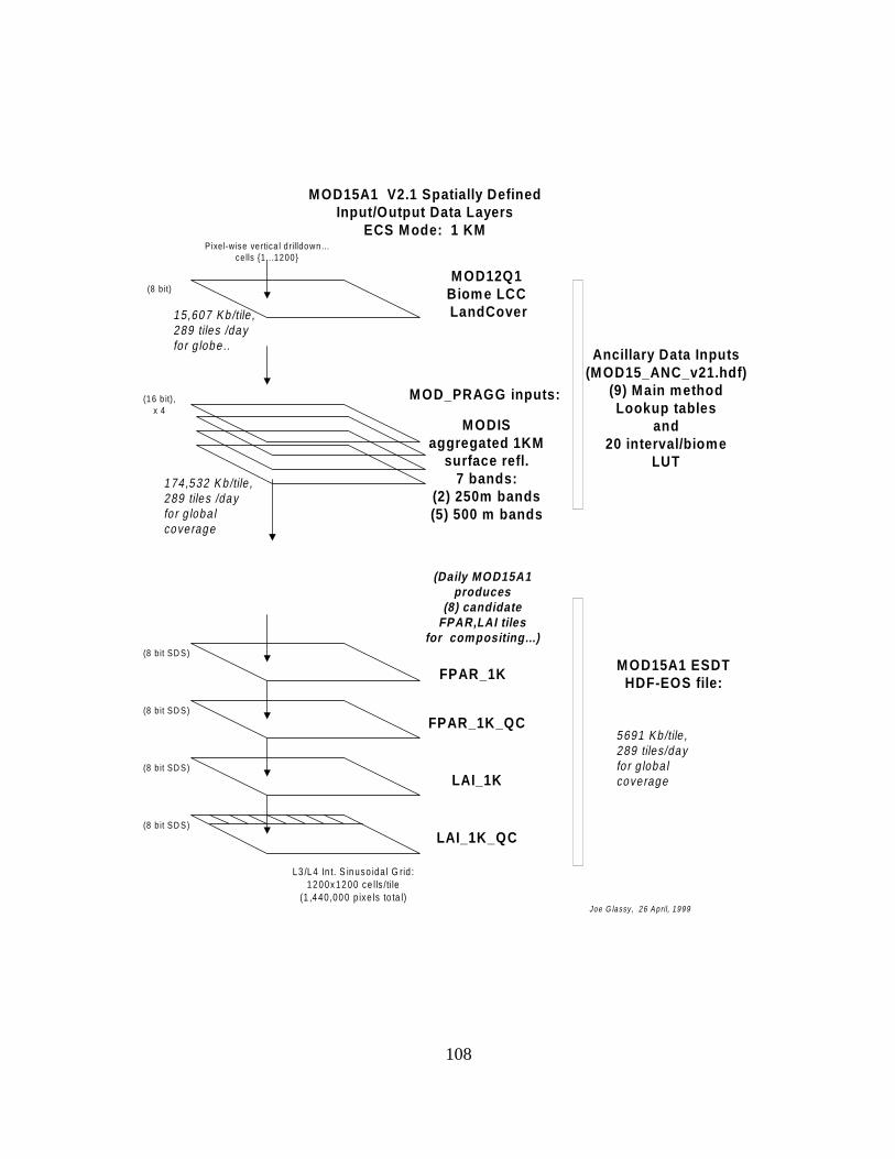
108

M OD12Q1Biome LCC LandCover

M ODISaggregated 1KM

surface refl.7 bands:

(2) 250m bands(5) 500 m bands

Ancillary Data Inputs(M OD15_ANC_v21.hdf)

(9) Main methodLookup tables

and20 interval/biome

LUT

M OD15A1 V2.1 Spatially DefinedInput/Output Data Layers

ECS M ode: 1 KM

Joe G lassy, 26 A p ril, 1999

FPAR_1K

FPAR_1K_QC

LAI_1K

LAI_1K_QC

Pixe l-w ise ve rtica l d rilldown ...ce lls 1 ...1200

L3 /L 4 In t. S in uso ida l G rid :12 00x 12 00 ce lls /tile

(1 ,4 40 ,00 0 p ixe ls to ta l)

(8 b it)

(16 b it),x 4

(8 b it SD S)

(8 b it SD S)

(8 b it SD S)

(8 b it SD S)

M OD_PRAGG inputs:

(Daily MOD15A1produces

(8) candidateFPAR,LAI tiles

for compositing...)

M OD15A1 ESDTHDF-EOS file:

174 ,532 K b /tile ,289 tiles /dayfo r g loba lcoverage

5691 Kb /tile ,289 tiles/dayfo r g loba lcoverage

15,607 Kb /tile ,289 tiles /dayfo r g lobe ..

109

6.2 Processing Issues

6.2.1 Processing Context

The key MODIS inputs to the MOD15A1 (PGE-33) and MOD15A2 (PGE-34) algorithmsare the 1KM land cover (MOD12Q1, gridfield "Land_Cover_Type1", and the aggregated 1KMsurface reflectance product (MOD_PRAGG: "Level 3 BRDF Preprocessing Database at 1kmresolution"). The daily 1KM surface reflectances are derived from the MOD09 250m and 500msurface reflectance product, and are atmospherically corrected. The following figure illustrates

MODIS MOD15 (FPAR,LAI)V2.1 At-Launch

PGE-33 and PGE-34 Data Flow Diagram

jm g , N T SG , 26 A p ril, 19 99

M OD_PRAGG1K M (7) band

surface reflectancein term ed iate p roduct

(w ith geom etry and Q A)

PGE-33M O D_PR15A1:

FPAR, LAIDa ily A lgorithm

M O D12Q1Land Cover C lasstiled data p roduct

(AT-LAUNCH)

PGE-34M O D_PR15A2:

FPAR, LAI8-day Com positing

A lgorithm

1 K F P A R8 -d a y C om p o s ite

G C T P_ IS IN U S

1 K F P A RD a ys 1 ...8

(G C T P _IS IN U S)

1 K L A ID a ys 1 ...8

(G C T P _IS IN U S)

1 K L A I8 -d a y C om p o s ite

G C T P_ IS IN U S

PGE-63M O D_PR15C:

FPAR, LAIM onth ly

CM G Algorithm

F P A R8 -d a y C M G5 6 K m res .

L A I8 -d a y C M G5 6 K m res .

da ily candida te tiles

M a in R -T d e riv e dF P A R , L A I

(9 )-P a rt L U T

P G E -33 H D F E O SF ie ld P ro pe r tie s

(T abu la r C o m pon en ts )

MOD15_ANC_v21.hdfH D F E O S v .2 .4 fo rm a t

(3 ,9 4 4 K b fi le )

D ire c t R e trie va l(2 0 in te rva ls /b io m e )

b a ck u p LU T

IS ti le g ridM B R c o o rd in a te s

110

the high level data flows for these algorithms:

6.2.2 Performance: MFLOPS and Storage Load Estimates

The at-launch computational metrics for MOD15A1 and MOD15A2 are shown in the tablebelow:

Computational Metrics: MFLOPS and Storage LoadsAlgorithm MFLOPS Storage Load (Gb/day)MOD15A1 (PGE-33) 7.009200 1.67 Gb/day (not archived)MOD15A2 (PGE-34) 0.000233 1.67 Gb/8-day period (archived)Totals: 7.001133 1.67 per 8-day period (archived)

Load Methods

IS grid tiles are classified as "land" when at least 1 or more 1KM pixel in the 0.50 degreetile region is classified as "land". For the daily storage load estimate, we assume (a worst case)that all (289) "land" tiles globally are produced daily, and that each product tile is 5,691 Kb insize (((5691 Kb/1000)*289 tiles)/1000=1.64 Gb/day.

MFLOPS Methods

The methodology used to estimate the MFLOPS is specific to the SGI 64 bit workstationclass (using the IRIX 6.4.x operating system), with 2 or more R10000 CPUs running at 195mhz.To obtain the MFLOPS estimate, we built and ran a special form of the algorithm on our SGIOctane (dual R10000,195mhz) workstation using the SGI IRIX "perfex" utility (e.g. for theMOD15A1.exe algorithm, we used:

perfex -a -mp -y >& MOD15A1_MFLOPS.report

Note that the MFLOPS value obtained from this utility technically refers to millions of floatingpoint instructions per second not millions of floating point operations per second, and due to thefact that there are sometimes multiple instructions per "operation", the value reported is notexact.

111

6.2.3 FPAR, LAI Algorithm Daily Logic (PGE-33)

The following section briefly summarizes the high-level runtime logic implemented inMOD15A1:

• Upon instantiation of the session (once per tile), the runtime inputs are retrieved from theprocess control file (.pcf) file provided by the high level scheduler/loader environment.

• The PGE allocates all in-memory data structures it requires, opens the static ancillaryHDFEOS file (MOD15_ANC_v21.hdf) and builds an in-memory dictionary of its contents.

• All spatial input HDFEOS files are opened (land cover and aggregated 1KM surfacereflectance files) and in-memory dictionaries are built of their contents.

• The daily candidate output file is created, using field properties read at runtime from theancillary file.

• A row-wise processing loop is established, and each subsequent row from all input files isbuffered into memory.

• A pixel-wise processing loop is established, and for each pixel, input fields are decoded fromtheir digital representation (integer) to their biophysical form (floating point) usinggain,offset calibration factors. QA fields from the inputs are also checked here, in order topass-through all pixels not classified as "land" or otherwise of unsuitable quality.

• The main R-T based retrieval method is performed on the pixel, using the channel-wisereflectances and pixel geometry. An FPAR, LAI estimate (and QA for each) is thencalculated for the pixel.

• The biophysical estimates are encoded to their digitial (integer) representations, and areplaced in the output buffer.

• When the current row is complete, it is written out to the open HDFEOS archive product file.• When all rows are complete, final ECS metadata processing is performed, whereby the ECS

metadata fields are set into their blocks, and finally written out to the product output file.• Final session cleanup tasks are then performed, where all dynamic memory is released, files

are closed.

6.2.4 FPAR, LAI Algorithm 8-day Compositing Logic (PGE-34)

The MOD15A2 (PGE-34) executable accepts a set of up to candidate tiles produced by thedaily MOD15A1 process, and composites these using a simple selection rule whereby the pixelwith the maximum FPAR (across the 8 days) is selected for inclusion in the output tile ofidentical format. Relevant QA and other tile-level metadata is taken from the day chosen tocontribute its primary FPAR. The same day chosen to represent the FPAR measure alsocontributes the pixels LAI value.

112

The MOD15A2 (PGE-34) executable is launched once every 8-day period, and is providedwith the current 8-day set of MOD15A1 candidate daily tile products. It performs the followingactions:

• Upon instantiation of the session (once per tile), the runtime inputs are retrieved from theprocess control file (.pcf) file provided by the high level scheduler/loader environment.

• The PGE allocates all in-memory data structures it requires; note this executable does notrequire the ancillary file, MOD15_ANC_v21.hdf.

• The set of 1-8 candidate daily MOD15A1 product files are opened, and in-memorydictionaries are built of their contents.

• A row-wise processing loop is established, and each subsequent row from each days inputfile is buffered into memory.

• A pixel-wise processing loop is established, and for each pixel, the raw digital values arestored.

• An inner-most, temporal loop is established, looping through the (1 to 8) days of candidatedata.

• From each set of 8 days pixels (e.g. using a vertical drill-down through the day dimension),the pixel with the highest FPAR value is identified. The base-0 index for this day is storedand used to retrieve the spatially coincident FPAR, LAI estimates associated with this day.

• The FPAR and LAI (and QC) values for the day identified above are then placed in the single2D output buffer at the appropriate line,sample position.

• When the current row is complete, it is written out to the open HDFEOS archive product file.• When all rows are complete, final ECS metadata processing is performed, whereby the ECS

metadata fields are set into their blocks, and finally written out to the product output file.• Final session cleanup tasks are then performed, where all dynamic memory is released, files

are closed.

6.3 Quality Assurance

6.3.1 Quality Control and Diagnostics

The level of attention to Quality Assurance tasks, on the whole, is expected to directlycorrelate with the usefulness of the EOS "Terra" AM-1 instrument data for terrestrial products.Thus, a considerable fraction of the output data is classified as "QA data". This contribution byQA activities is matched within the algorithm logic itself: a significant portion of the logic isdedicated to verifying the quality of the internal data pipeline. In total, the QA subsystem withan algorithm represents some complex data flows, since input data from "upstream" is alsosupplied with both tile and pixel-level QA data and must be appropriately evaluated in the courseof our PGE33 process.

113

The QA information in NASA EOS product files is loosely classified as "metadata", ordata about data. Tile level metadata fields are further divided into Earth Observing SystemDistributed Information System (EOSDIS) Core System (ECS) metadata fields, and SCFsupplied metadata. ECS metadata fields will be archived in separate NASA databases, and areconsidered "searchable" metadata, in that tools will be provided to users to allow them to searchand filter tiles on the basis of the appropriate ECS metadata fields.

Within the group of ECS "searchable" metadata fields, an additional category is offeredcalled product specific metadata (PSA). These are additional, special metadata fields unique toeach Earth Science Data Type (ESDT) or product. Each type of metadata component plays animportant role and are processed somewhat differently. All metadata fields are also fullydescribed in the given ESDT's file specification. The ECS metadata fields are organized withinone of (3) compound (character) attributes stored at the top logical level within HDFEOS files.These are:

• "StructMetadata.0" (HDFEOS grid specific and map projection parameters)• "CoreMetadata.0" (Core metadata)• "ArchiveMetadata.0" (Archive metadata)

The StructMetadata.0 field contains a number of map projection related parametersrelevant to the product file. The CoreMetadata.0 block contains a set of browse-able metadatafields that will eventually serve as selection criteria for users ordering the data, and theArchiveMetadata.0 block contains a number of system parameters, such as the limits of the tile'sspatial extent (in geodetic coordinates), the granule day/night beginning and ending date andtimes, etc.

Tile level metadata fields within these large compound text blocks are further organizedusing the NASA Object Data Language(ODL)/Parameter Value Language (PVL) objecthierarchy scheme. A special set of software functions --the "MET" subsection of the SoftwareData Production Toolkit (SDPTK) library -- are used to perform all manipulations on ECSmetadata fields within this hierarchy. The user may discover all the metadata associated with agiven product by referring to:

• The product's "MCF" file (ours is MOD15A1.mcf). In this structured text file all the ECSmetadata fields (archived, searchable, and PSA) are enumerated along with most of theirdefining properties.

• The MOD15A2 archive product's file specification (MOD15A2.fs), which describes allaspects of a given ESDT product, including the number, layout of primary data planes in anHDFEOS file, as well as the full set of metadata fields (ECS and SCF).

114

• Refer to NASA web sites dedicated to ECS metadata information base: e.g. the Users mayrefer to a very complete information base on the ECS metadata concepts may be found at:http://ecsinfo.hitc.com/metadata/metadata.html

We define a number of product specific (PSA) attributes, stored in the CoreMetadata.0block, set under the internal name ADDTIONALATTRIBUTES. Refer to the table describingthese in detail, in the section below titled Output Product.

The PGE33 (daily MOD15A1) and PGE 34 (8-day composite MOD15A2) pixel wise QAinformation consists of a single 8-bit unsigned character compound bit-field, organized asfollows:

MOD15A1/MOD15A2 PGE33 QA Pixel DescriptionsBit Field Bits Range Bit-code DefinitionsMODLAND QA 00-01 00-11 00= Product pixel produced at ideal

quality,01= Product pixel produced, less thanideal quality10= Product pixel not produced due tocloud effects11=Product pixel not produced for otherreason

ALGORITHM_PATH 02-03 00-11 00= pixel could not be calculated usingany method (usually due to missing or badinputs)01=calculate using main Boston method10=calculated using backup method

PGE33: not used v.2.1 04-05 00-11FPAR,LAI SummaryQA

06-07 00-11 00= Highest quality (76-100 percentilequality score)01= Good quality (49-75 percentilequality score)10= Poor or Questionable quality (26-50percentile score)11= Unacceptable quality, (0-25)recommend avoid using

We anticipate that the official NASA data ordering tool(s) will incorporate methods bywhich users may mask (e.g. define selection criteria) for tiles of interest using variouscombinations of these pixel level flags.

115

6.3.2 Pixel Level Qualification Criteria and Selection Logic

PGE33 subjects each input pixel to an independent qualification test based on thecollective QA for the MODAGAGG data supplied. The result of the series of tests is that theinput pixel is scored on a simple 4-level scale. These levels are:

Univ.Montana SCF 4-Level QA ScoresCode Value DefinitionIsQaBestQuality 0 Best possible, preferred qualityIsQaMinAcceptQuality 1 Minimum acceptable qualityIsQaBadQuality 2 Poor quality, not recommended for use (not proc)IsQaWorstQuality 3 Worst possible, pixel not processed further.

All input-pixel level QA logic is implemented in the lai_tran_input_pix() function in thelai_tran.c module file. The logic used in the series of pixel-wise tests is summarized next, byorder of the test:

1. The UMD Land Cover class code is first converted from the original UMD (18 or 14) classscheme to the University of Montana/Boston Univ. (7) biome classification. Note that UMbiome code 0 is water/rock and code 7 is barren--pixels with these types are not processedfurther.

2. If the converted biome class lies in the range 1,2,3,4,5,6, processing continues for thepixel; otherwise, fill values are placed in the output buffer to indicate that the pixel is notprocessed, and appropriate ECS metadata fields are set accordingly.

3. Next, the MODAGAGG aggregate QC bits are parsed and analyzed. If the cloud bit equals 1(is too cloudy), or the LandWater bit is != 1, (e.g. is NOT land) the FPAR, LAI QC bits areset to IsQaWorstQuality, and the pixel is not processed.

4. Next, the pixel is checked to see if it meets the minimum quality threshold. This is true isany of the following conditions are met:a) the cloud bit is >= 1 ( e.g. mixed or assumed not set)b) the cirrus bit is >=2 (e.g. average or high amount of cirrus)c) the cloud shadow bit ==1 (e.g. pixel is in cloud shadow)d) the aerosol bit ==3 (e.g. a high amount of aerosol has been encountered)e) the snow/ice bit must be 0 (e.g. snow/ice does not occupy a significant portion of the

pixel)

116

5. The 1KM aggregated surface reflectances for all channels used (2 or 4) are then unpacked,along with their pixel level QC bits, and are then further analyzed. If the MODLAND bitsare > 1 or the Atmosphere bit is >= 13, the pixel is rated IsQaWorstQuality and processing isblocked for the pixel. A check is then made on how many of the individual bands used (2 or4) supplied inputs at the level of IsQaMinAcceptQuality or better. For the main method to beused, all 2 or 4 bands must have supplied this level of quality. If even one band suppliedinferior quality inputs, then the main method is blocked, and a flag is set indicating that thebackup method should be tried instead, provided that the first (2) bands of input --theminimum required for the backup method-- were scored at the level ofIsQaMinAcceptQuality or better.

6.3.3 Exception Handling

Exception handling for the MOD15A1 (PGE-33) and MOD15A2 (PGE-34) is performed usingthe standard ECS compliant SDTPK SMF software layer. In our implementation of thismethod, we define (4) classes of exceptions according to their severity. A common SMFmessage file is used for all our algorithms (PGS_MODIS_37150.t/.h). The single letter severitycodes U,W,E,F were adapted from the SDPTK User's Guide, Section 6.128. The table belowsummarizes these:

Univ. Montana SCF Exception Handling (PGE_MODIS_37150.t symbols)Message Code Severity CommentsMODIS_U_MUM_ADVISORY Advisory These messages are used to

passively inform the operator oruser about a given condition.

MODIS_W_MUM_ADVISORY Warning These messages indicate that anout of the ordinary conditionhas occurred, that may requiremonitoring further.

MODIS_E_MUM_ADVISORY Error These messages indicate that a(non-fatal) program error hasoccurred which should beinvestigated as soon as possible.

MODIS_F_MUM_ADVISORY Fatal exception These messages indicate that afatal program error or conditionhas been encountered. ThePGE will halt shortly afterperforming as much damage-containment as it can.

Generally, when an exception of class MODIS_F_MUM_ADVISORY is encountered, thiswill necessitate re-running the PGE against the indicated tile, once the cause has been identified

117

and a solution has been determined. A single "collector" exception handling call is madewhenever any of these exceptions is encountered. This call routes the text of the message to the(3) standard SDPTK session log files, e.g. (MOD15_StatusLog.log, etc). An example of such acall is shown below:

mum_message(MODIS_U_MUM_ADVISORY,"lai_main.c","lai_driver","Pixels successfully processed %ld\n",n_total);

6.3.4 Output Product Details

The MOD15A1 (PGE-33) daily executable produces IS tile (NASA HDFEOS v.2.4format) output files that are formally identical to the archived 8-day product generated byMOD15A2. The full baselined file format for these may normally be found at:

ftp://modis-xl.nascom.nasa.gov/modisbaselinedcode/COMMON/filespec

To summarize the contents of the archived MOD15A2 FPAR, LAI product file, it contains(4) spatially defined 2D gridfields, the full set of ECS Core, Archive, and Struct metadata fieldsin Parameter-Value-Language (PVL)/Object Data Language (ODL) format blocks, as well as asmall set of gridfield (or SDS) attributes. Note that HDF and HDF-EOS format files use anunderlying "xdr" based numeric representation for data, which allows data of any numeric datatype to be ported to virtually any compute platform, regardless of the "endian" byte-ordering ofthe native word on the platform. The common datatype the main gridfields are stored in (e.g.DFNT_UINT8) is a platform independent, unsigned, 8-bit integer type capable of representingnumeric values in the range 0 <= dn <= 255 inclusive. The (4) main gridfields aresummarized further in the following table:

MOD15A2 FPAR, LAI 8-day composite archive file summaryGrid Field Name Datatype Dimensions DescriptionFpar_1km DFNT_UINT8 1200 x 1200 spatial FPAR fieldLai_1km DFNT_UINT8 1200 x 1200 spatial LAI fieldFpar_1km_QC DFNT_UINT8 1200 x 1200 Pixel-wise quality control for the

modeled FPAR measure.Lai_1km_QC DFNT_UINT8 1200 x 1200 Pixel-wise quality control flags

for the LAI measure.

Users may refer to a very complete information base on the ECS metadata concepts maybe found at: http://ecsinfo.hitc.com/metadata/metadata.html

118

A set of ECS compliant Product Specific Attributes (PSA) is also included in each tile file,within the CoreMetadata.0 block. These provide users with a very coarse but quick "tile-level"quality assessment for the product file. The table below summarizes these:

MOD15A2 (PGE 34) Archive Product Specific AttributesPSA Metadata Field Name Field DescriptionN_DAYS_COMPOSITED PGE33 always 1; PGE34 this is the number of

days contributing to the final composite.QAPERCENTGOODFPAR Percent 0<=p<=100 of FPAR pixels rated at

good (e.g. IsQaMinAcceptQuality ) or betterQAPERCENTGOODLAI Percent 0 <= p <= 100 of LAI pixels rated at

good (IsQaMinAcceptQuality) or better.QAPERCENTMAINMETHOD Percent 0 <= p <= 100 of pixels calculated

using main methodQAPERCENTEMPIRICALMETHOD Percent 0 <= p <= 100 of pixels calculated

using backup method (reciprocal of above)TILEID IS Tile ID code, an 8-digit integer that

identifies the map projection used, the tile'ssize code (quarter, half, or full-tile) and thetile's horizontal and vertical position in thegrid.

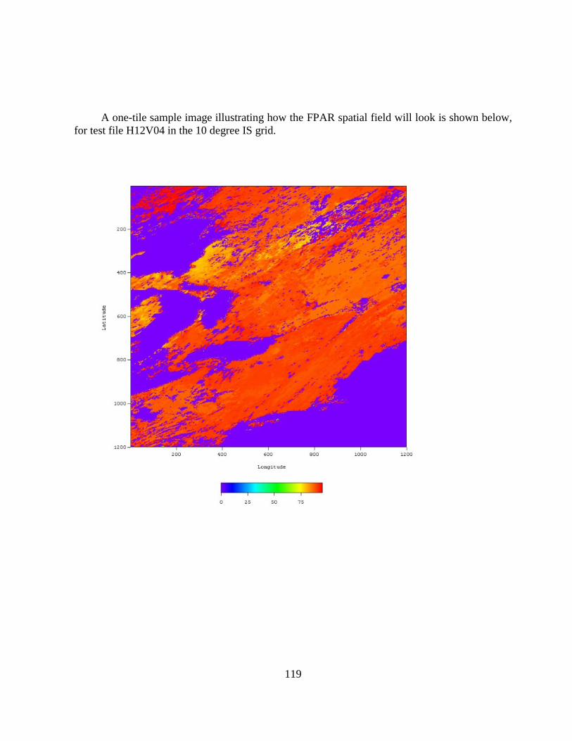
119

A one-tile sample image illustrating how the FPAR spatial field will look is shown below,for test file H12V04 in the 10 degree IS grid.

120

A one-tile sample image illustrating how the LAI spatial field will look is shown below,for test file H12V04 in the 10 degree IS grid.

121

REFERENCES

Anisimov, O. A., and G. V. Menzulin, The problem of modeling the radiative radiation regime inthe plant cover, Sov. Meteorol. and Hydrol., 10, 70-74, 1981.

Asrar, G., M. Fuchs, E.T. Kanemasu, and J.L.Hatfield, Estimating absorbed photosyntheticradiation and leaf area index from spectral reflectance in wheat, Agron. J., 76, 300-306,1984.

Baret, F., S. Jacquemoud, and J.F. Hanocq, The soil concept in remote sensing, Remote Sens.Rev., 7, 65-82, 1993.

Barnsley, M. F., Fractals Everywhere, 531 pp., Academic, San Diego, Calif., 1993.

Bass, L.P., A.M.Volocsvhenko, and T.A.Germogenova, Methods of Discrete Ordinates inRadiation Transport Problems (in Russian, with English abstract), 231 pp., Inst. Appl.Math., Russ. Acad. of Sci., Moscow, 1986.

Belward, A.S. and Loveland, T.R., The IGBP-DIS 1-km land cover project. Proceedings, RSS'95Remote Sensing in Action, 21st Annual Conference of the Remote Sensing Society,Southhampton, UK, 11-14 September 1995 (Nottingham: Remote Sensing Society), pp.1099-1106, 1995.

Borel, C.C., S.A., Gerstl, and B.J. Powers, The radiosity method in optical remote sensing ofstructured 3-D surfaces, Remote Sens. Environ., 36, 13-44, 1991.

Chen. J. M, Canopy architecture and remote sensing of the fraction of photosynthetically activeradiation absorbed by boreal conifer forests, IEEE Trans. Geosci. Remote Sens., 34,1353-1368, 1996.

Chen. J. M and Jose Cihlar, Retrieving leaf area index of boreal conifer forests using landsatTM images, Remote Sens. Environ., 55, 153-162, 1996.

Cihlar, J, J. Chen, and Z. Li, Seasonal AVHRR multichannel data sets and products for studiesof surface-atmosphere interactions, J. Geophys. Res., 102, 29625-29640, 1997.

Clevers, J. G. P. W, The application of a weighted infrared-red vegetation index for estimatingleaf area index by correcting for soil moisture, Remote Sens. Environ., 29, 25-37, 1989.

Deschamps, P.Y., F.M. Bréon, M. Leroy, A. Podaire, A. Bricaud, J.C. Buriez, and G. Sèze, ThePOLDER mission: Instrument characteristics and scientific objectives, IEEE Trans.Geosci. Remote Sens., GE-32, 598-615, 1994.

Diner, D.J., J.V.Martonchik, C. Borel, S.A.W. Gerstl, H.R. Gordon, Y. Knyazikhin, R. Myneni,B. Pinty, and M.M. Verstraete, MISR: Level 2 surface retrieval algorithm theoretical basis,JPL Internal Doc. D-11401, Rev. C, Calif. Inst. of Technol., Jet Propul. Lab., Pasadena,1998a.

122

Diner, D.J., W.A. Abdou, H.R. Gordon, R.A. Kahn, Y. Knyazikhin, J.V.Martonchik, S.McMuldroch, R.B. Myneni, and R.A. West, Level 2 ancillary products and data setsalgorithm theoretical basis, JPL Internal Doc. D-13402, Rev. A, Calif. Inst. of Technol., JetPropul. Lab., Pasadena, 1998b.

Eisen, M., Introduction to Mathematical Probability Theory, 535 pp., Prentice Hall, EnglewoodCliffs, New Jersey, 1969.

GCOS/GTOS, GHOST-global hierarchical observing strategy, GCOS-33, WMO-No. 862, WorldMeteorol. Org., Geneva, 1997.

Germogenova, T.A., The Local Properties of the Solution of the Transport Equation (inRussian), 272 pp., Nauka, Moscow, 1986.

Hansen, M.C., DeFries, R.S., Townshend, J.R.G. and Sohlberg, R., Global land coverclassification at 1km spatial resolution using a classification tree approach, InternationalJournal of Remote Sensing, Submitted, 1999.

Holben, B. N, Characteristics of maximum-value composite images from temporal AVHRRdata, Int. J. Remote Sens., 7, 1417-1434, 1986.

Jacquemoud, S., F. Barret, and J.F. Hanocq, Modeling spectral and bidirectional soil reflectance,Remote Sens. Environ., 41, 123-132, 1992.

Justice, C., D. Starr, D. Wickland, J. Privette and T. Suttles, EOS land validation coordination:an update, Earth Observer, 10(3):55-60, 1998.

Kimes, D.S., Radiative transfer in homogeneous and heterogeneous vegetation canopies, inPhoton-Vegetation Interactions: Applications in Plant Physiology and Optical RemoteSensing, pp. 339-388, edited by R. B. Myneni and J. Ross, Springer-Verlag, New York,1991.

Knyazikhin, Y., and A. Marshak, Fundamental equations of radiative transfer in leaf canopiesand iterative methods for their solution, in Photon-Vegetation Interactions: Applications inPlant Physiology and Optical Remote Sensing, pp. 9-43, edited by R. B. Myneni and J.Ross, Springer-Verlag, New York, 1991.

Knyazikhin, Y., J. Kranigk, G. Miessen, O. Panfyorov, N. Vygodskaya, and G. Gravenhorst,Modelling three-dimensional distribution of photosynthetically active radiation in slopingconiferous stands, Biomass Bioenerg., 2/3, 189-200, 1996.

Knyazikhin, Y., G. Mießen, O. Panfyorov, and G. Gravenhorst, Small-scale study of three-dimensional distribution of photosynthetically active radiation in a forest, Agric. For.Meteorol., 88, 215-239, 1997.

Knyazikhin, Y., J.V., Martonchik, R.B. Myneni, D.J. Diner, and S.W. Running, Synergisticalgorithm for estimating vegetation canopy leaf area index and fraction of absorbedphotosynthetically active radiation from MODIS and MISR data, J. Geophys. Res., 103,D24, 32,257-32,275, 1998a.

123

Knyazikhin, Y., J.V. Martonchik, D.J.Diner, R.B. Myneni, M.M. Verstraete, B.Pinty, and N.Gobron, Estimation of vegetation canopy leaf area index and fraction of absorbedphotosynthetically active radiation from atmosphere-corrected MISR data, J. Geophys.Res., 103, D24, 32,239-32,256, 1998b.

Knyazikhin, Y., J. Kranigk, R.B. Myneni, O.Panfyorov, and G.Gravenhorst, Influence of small-scale structure on radiative transfer and photosynthesis in vegetation cover, J. Geophys.Res., 103, 6133-6144, 1998c.

Kolmogorov, A.M., Foundations of the Theory of Probability, 71 pp., Chelsea, New York, 1950.

Kondratyev, K. Y., Radiation in the Atmosphere, 912 pp., Academic, San Diego, Calif., 1969.

Kranigk, J., Ein Model für den Strahlungstransport in Fichtenbeständen, 127 pp., Cuvillier,Göttingen, Germany, 1996.

Krein, S.G (Ed.), Functional Analysis, 352 pp., Foreign Technol. Div., Wright-Patterson AirForce Base, Ohio, 1967.

Kuusk, A., The hot spot effect of a uniform vegetative cover, Sov. J. Remote. Sens., 3, 645-658,1985.

Lebesgue, H., Intégrale, Longueur, Aire, Thése (Paris 1902) ou Annali Mat Pura e Appl., vol. 3,Nr. 7, 231-359, 1902.

Li, X., and A.H. Strahler, Geometrical-optical bidirectional reflectance modeling of the discretecrown vegetation canopy: Effect of crown shape and mutual shadowing, IEEE Trans.Geosci. Remote Sens., 30, 276-292, 1992.

Li, X., and A. Strahler, Geometric-optical modeling of a coniferous forest canopy, IEEE Trans.Geosci. Remote Sens., GE-23, 207-221, 1985.

Li, X., A. Strahler, and C. E. Woodcock, A hybrid geometric optical-radiative transfer approachfor modelling albedo and directional reflectance of discontinuous canopies, IEEE Trans.Geosci. Remote Sens., 2, 466-480, 1995.

Liou, K.-N., An Introduction to Atmospheric Radiation, 392 pp., Academic, San Diego, Calif.,1980.

Loveland, T. R., Merchant, J. W., Brown, J. F., Ohlen, D. O., Reed, B. C., Olsen, P. andHutchinson, J., Seasonal land cover of the United States, Annals of the Association ofAmerican Geographers 85(2), 339-355,1995.

Loveland, T.R. and Belward, A.S., The IGBP-DIS global 1km land cover data set, DISCover:first results, International Journal of Remote Sensing 18, 3289-3295, 1997.

Marshak, A., Effect of the hot spot on the transport equation in plant canopies, J. Quant.Spectrosc. Radiat. Transfer, 42, 615-630, 1989.

Martonchik, J.V., D.J. Diner, B. Pinty, M.M. Verstraete, R.B. Myneni, Y. Knyazikhin, and H.R.Gordon, Determination of land and ocean reflective, radiative and biophysical propertiesusing multi-angle imaging, IEEE Trans. Geosci. Remote Sens., 36, 1266-1281, 1998.

124

Myneni, R.B., Modeling radiative transfer and photosynthesis in three-dimensional vegetationcanopies, Agric. For. Meteorol., 55, 323-344, 1991.

Myneni, R. B., and G. Asrar, Photon interaction cross sections for aggregations of finitedimensional leaves, Remote Sens. Environ., 37, 219-224, 1991.

Myneni, R. B., and D. L. Williams, On the relationship between FAPAR and NDVI, RemoteSens. Environ., 49, 200-211, 1994.

Myneni, R.B., J. Ross, and G. Asrar, A review on the theory of photon transport in leaf canopiesin slab geometry, Agric. For. Meteorol., 45, 1-165, 1989.

Myneni, R.B., A.L. Marshak, and Y. V. Knyazikhin, Transport theory for a leaf canopy of finite-dimensional scattering centers, Quant. Spectrosc. Radiat. Transfer, 46, 259-280, 1991.

Myneni, R.B., F.G. Hall, P.J. Sellers, and A.L. Marshak, The interpretation of spectral vegetationindexes, IEEE Trans. Geosci. Remote Sens., 33, 481-486, 1995a.

Myneni,R.B., S. Maggion, J. Iaquinta, J.L.Privette, N. Gobron, B. Pinty, D.S. Kimes, M.M.Verstraete, and D.L. Williams, Optical remote sensing of vegetation: Modeling, caveatsand algorithm, Remote Sens. Environ, 51, 169-188, 1995.

Myneni, R.B., R.R. Nemani, and S.W. Running, Estimation of global leaf area index andabsorbed PAR using radiative transfer model, IEEE Trans. Geosci. Remote Sens., 35, 1380-1393, 1997.

Myneni,R.B., C.D. Keeling, C.J. Tucker, G.Asrar, and R.R. Nemani, Increased plant growth inthe northern high latitudes from 1981 to 1991, Nature, 386, 698-702, 1997a.

Myneni, R.B., R.R. Nemani, and S.W. Running, Estimation of global leaf area index andabsorbed PAR using radiative transfer model, IEEE Trans. Geosci. Remote Sens., 35, 1380-1393, 1997b.

Nilson, T., A theory of radiation penetration into non-homogeneous plant canopies, in ThePenetration of Solar Radiation into Plant Canopies (in Russian), pp. 5-70, Estonian Acad.of Sci., Tartu, 1977.

Norman, J.M., and J. M. Welles, Radiative transfer in an array of canopies, Agron. J., 75, 481-488, 1983.

Oker-Blom, P., J. Lappi., and H. Smolander, Radiation regime and photosynthesis of coniferousstands, in Photon-Vegetation Interactions: Applications in Plant Physiology and OpticalRemote Sensing, pp. 469-499, edited by R. B. Myneni and J. Ross, Springer-Verlag, NewYork, 1991.

Peterson, D. L, M. A. Spanner, S. W. Running, and L. Band, Relationship of ThematicMapper Simulator data to leaf area index, IEEE Trans. Geosci. Remote Sens., 22, 323-341, 1987.

Pinty, B., and M.M. Verstraete, Modeling the scattering of light by vegetation in optical remotesensing, J. Atmos. Sci., 55, 137-150, 1998.

125

Pinty, B., M.M.Verstraete, and R.E.Dickenson, A physical model for predicting bidirectionalreflectance over bare soils, Remote Sens. Environ., 27, 273-288, 1989.

Pokrowski, G.I., Über die Helligkeitsverteilung am Himmel (in German), Phys. Z., 30, 697-700,1929.

Privette, J. L., R. B. Myneni, W. L. Emery, and C. J. Tucker, Invertibility of a 1D discreteordinates canopy reflectance model, Remote Sens. Environ., 48, 89-105, 1994.

Privette, J., R. Myneni, J. Morisette and C. Justice, Global validation of EOS LA1 and FPARproducts, Earth Observer, 10(6):39-42, 1998.

Privette, J.L. and G.P. Asner, The prototype validation exercise (PROVE) for EOS land andatmosphere products, IGARSS’99 Proceedings (99.110 1), 1999.

Ross, J., The Radiation Regime and Architecture of Plant Stands, 391 pp., Dr. W. Junk, Norwell,Mass., 1981.

Ross, J.K., and A. L. Marshak, Calculation of the solar radiation reflection from plant coverusing the Monte-Carlo method, Sov. J. Remote. Sens., 5, 58-67, 1984.

Ross, J., and T. Nilson, A mathematical model of radiation regime of plant cover, in Actinometryand Atmospheric Optics (in Russian), Valgus, Tallin, Estonia, 1968.

Ross, J., Y. Knyazikhin, A. Kuusk, A. Marshak, and T. Nilson, Mathematical Modeling of theSolar Radiation Transfer in Plant Canopies (in Russian, with English abstract), 195 pp.,Gidrometeoizdat, St. Peterburg, Russia, 1992.

Running, S.W., R.B. Myneni, R. Nemani, J. Glassy, MOD15 LAI/FPAR algorithm theoreticalbasis document, MODIS LAI (leaf area index) and MODIS FPAR (fraction of absorbedphotosynthetically active radiation), Tech. Rep., Sch. of For., Univ. of Mont., Missoula,1996.

Sellers, P.J., J.A. Berry, G.J. Gollatz, C.B.Field, and F.G. Hall, Canopy reflectance,photosynthesis and transpiration, III, A reanalysis using improved leaf models and a newcanopy integration scheme, Remote Sens. Environ., 42, 187-216, 1992.

Sellers, P.J., et al., Modeling the exchange of energy, water, and carbon between continents andatmosphere, Science, 275, 602-509, 1997.

Simmer, C., and S.A. Gerstl, Remote sensing of angular characteristics of canopy reflectances,IEEE Trans. Geosci. Remote Sens., GE-23, 648-658, 1985.

Titov, G.A., Statistical description of radiative transfer in clouds, J. Atmos. Sci.,47, 24-38, 1990.

Tucker, C.J., Red and photographic infrared linear combination for monitoring vegetation,Remote Sens. Environ., 8, 127-150, 1979.

Tucker, C. J, P. J. Sellers, Satellite remote sensing of primary production, Int. J. RemoteSens., 7, 1395-1416, 1986.

126

Tucker, C.J., Y.Fung, C.D. Keeling, and R.H. Gammon, Relationship between atmospheric CO2

variations and a satellite-derived vegetation index, Nature, 319, 195-199, 1986.

Vainikko, G.M, Equation for mean intensity in broken clouds (In Russian), Meteorol. Issled., 21,28-37, 1973.

Verma, S. B, P. J. Sellers, C. L. Walthall, F. G. Hall, J. Kim and S. J. Goetz,Photosynthesis and stomatal conductance related to reflectance on the canopy scale,Remote Sens. Environ., 44, 103-116, 1993.

Vermote, E., L. A. Remer, C. O. Justice, Y. J. Kaufman, and D. Tanré, Atmospheric correctionalgorithm: Spectral reflectances (MOD09), version 2.0, Algorithm technical backgrounddocument, NASA EOS-ID 2015 Doc., 42 pp., 1995.

Verstraete, M.M., and B. Pinty, Designing spectral indexes for remote sensing applications,IEEE Trans. Geosci. Remote Sens., 34, 1254-1265, 1996.

Verstraete M.M., B. Pinty, and R.E. Dickenson, A physical model of the bidirectional reflectanceof vegetation canopies, J. Geophys. Res., 95, 11765-11775, 1990.

Vladimirov, V.S., Mathematical problems in the one-velocity theory of particle transport, Tech.Rep. AECL-1661, At. Energy of Can. Ltd., Chalk River, Ontario, 1963.

Vygodskaya, N.N., and I.I. Gorshkova, Theory and Experiment in Vegetation Remote Sensing (inRussian, with English abstract), 248 pp., Gidrometeoizdat, St. Petesburg, Russia, 1987.