Abstract — In this paper, an algorithm for the reconstruction

of an outdoor environment using a mobile robot is presented.

The focus of this algorithm is making the mapping process

efficient by capturing the greatest amount of information on

every scan, ensuring at the same time that the overall quality of

the resulting 3D model of the environment complies with the

specified standards. With respect to existing approaches, the

proposed approach is an innovation since there are very few

information based methods for outdoor reconstruction that use

resulting model quality and trajectory cost estimation as

criteria for view planning.

I. INTRODUCTION

3D modelling of large environments has become a matter

of increasing interest in recent years due to its multiple

application fields, such as reverse architecture, archaeology,

public works or multimedia presentations, among others.

This is possible thanks to recent advances in laser scanning

technology and related 3D processing algorithms. Laser

devices permit automatic scanning of the environment to the

desired resolution and measure the geometric coordinates

(x,y,z) of every point travelled across by the laser beam,

with respect to the scanner location.

However, setting up a typical stationary laser scanning

scheme is a difficult and time consuming labour. These

devices are usually heavy and require the set up of many

different pieces of equipment (tripod, batteries, GPS antenna

and computer). Moreover, a human operator has to choose

which views will be less occluded and will provide more

information and has to decide when the number of scans is

large enough to cover the complete model. All this is done

usually upon operator experience, without taking a close

look at the resulting model.

The use of mobile robots equipped with on board 3D

scanning systems emerges as a suitable alternative, ([1], [2],

[3]) given that robots provide mobility, computing system,

physical support to the scanner and positioning sensors.

However, though the use of mobile robots reduces greatly

the effort involved in the scanning process, the automation

of the view selection is still an open problem.

This issue has been addressed within the field of mobile

robot exploration. Most research effort has been focussed on

the SLAM (Simultaneous Localization and Mapping)

problem, and the developed techniques are designed to

This research has been supported by the Science and Innovation Spanish ministry (Pr.

Nb.DPI2008-06738-C02-01/DPI ), and the Consejería de Educación of the Junta de

Castilla y León (Pr. Nb. VA001A10-2).

The first author is with CARTIF Centro Tecnológico, Dep. Of Robotics and Computer

Vision, Boecillo (Valladolid, Spain); email: { jaipul@cartif.es }.

The second and third authors are with the University of Valladolid (Spain), Dep. Of

Systems Engineering and Automatic Control, Industrial Engineering School; email:

{ezalama@eis.uva.es, jaigom@cartif.es }

improve relevant feature extraction along robot trajectories

in order to maximize robot localizability and map

information. Usually, the main objective of these approaches

is to obtain indoor maps which help robots to self localise,

and mapping process is reduced to the x-y dimensions.

Outdoor environments have many characteristics that make

the problem different form indoor case. The environment is

less structured: it is not restricted by walls, the floor is not

plain, there are arbitrary but relevant 3D elements (such as

trees, stones and cars), and thus 2D maps are not efficient for

navigation purposes. Moreover, 3D mapping is a more

complex problem due the huge memory and computational

resources required for data handling, besides of other

problems such as occlusions. Fortunately, the localization

problem is less severe in outdoor environments due the

availability of absolute localization sensors like DGPS and

compasses, which provide reasonably accurate robot

localization.

Under these circumstances, the algorithm presented in this

paper is focused on optimizing the exploration process by

maximizing the map quality, while reducing the amount of

scans required for creating a good quality 3D model of the

environment. The goal is to have a robot that can build a

model of its surrounding environment in an efficient way, so

this robot has to consider previous data to choose the best

next locations to carry out a new scan, and compute the

trajectory towards these locations. This methodology can be

applied to most outdoors scenes such as urban locations,

monuments, archaeological sites and forest.

II. PREVIOUS WORK

Several exploration techniques have been proposed in the

literature, following two main strategies: strategies where a

given trajectory or behaviour (e.g. wall following or moving

to random positions) is defined upon a priori information of

the environment ([4], [5]), and strategies that predict which

movement will improve the most the robot knowledge of the

environment, based on acquired information.

The first group of strategies lacks adaptability to unknown

environment, where they tend to either leave unexplored

areas or be highly inefficient. Therefore, the second group of

strategies has received more attention since environment

information is used to decide further actions and they are

more adaptable to any kind of environment. In general

methods belonging to this second group are known as next

best view (nbv) given that their focus is to find the best next

observation position.

Common methods within nbv approaches are greedy

methods [6], where the robot moves to the closest location of

interest; frontier based methods [7], where candidate

Jaime Pulido Fentanes*, Eduardo Zalama**, Jaime Gómez-García-Bermejo**, *CARTIF Foundation, **Instituto Tecnologías de la Producción (ITAP), Universidad de Valladolid

Algorithm for Efficient 3D Reconstruction of Outdoor

Environments Using Mobile Robots

locations are generated on the frontier between the explored

and unexplored areas; and information based strategies that

use evaluation functions where different criteria is employed

to choose the next best position according to the selected

criteria, for example traveling cost [8].

Among the information based works, some of them use

functions to predict the utility of a given location. For

example, in [9] the utility of a target location is defined as an

expected information gain. In [10] traveling cost is

combined with information gain so that the next best view

point is chosen to maximize coverage and reduce traveling

distance. Some strategies find interest areas within the map

that are also used as a criteria, for example in [11] relevant

features within the map are included and used for evaluating

next best view considering that seeing these regions will

facilitate SLAM.

For 3D mapping, [12] proposes a hierarchical nbv method

for quickly evaluating multiple 3D views in indoor scenarios

using model quality and completeness as criteria, this work

presents different algorithms to efficiently evaluate several

viewpoints with respect to large sets of 3D data where

different where positioning and sensing constraints are taken

into account. A different solution for outdoor 3D mapping is

proposed in [13], where a 2D floor map of the area to be

scanned is used to find possible occlusions that a 3D scan

would have from different floor points. The combination of

viewpoints that requires the lowest number of scans to

entirely cover the target area is then found upon this process.

Once a 3D scan has been taken from each previously

calculated viewpoint, a view planning algorithm is used to

cover all unpredicted occlusions on the model with as few

scans as possible.

III. THE EXPERIMENTAL FRAMEWORK

The proposed algorithm has been designed for an all-

terrain robot we have developed for outdoor 3D

reconstruction (Fig. 1). This robot has a six wheel

differential traction system, an electronic traction control

system, an on-board PC system, and a multi-channel, long-

range communication system for teleoperating or monitoring

the robot in autonomous and semi-autonomous missions, as

well as different navigation sensors (cameras, laser, GPS and

IMU).

Fig. 1: All-terrain Robot developed by CARTIF

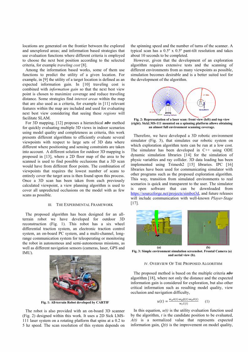
The robot is also provided with an on-board 3D scanner

(Fig. 2) designed within this work. It uses a 2D Sick LMS-

111 laser system on a rotating platform that spins at a 0.2 to

5 hz speed. The scan resolution of this system depends on

the spinning speed and the number of turns of the scanner. A

typical scan has a 0.5º x 0.5º pant-tilt resolution and takes

about 10 seconds to be completed.

However, given that the development of an exploration

algorithm requires extensive tests and the scanning of

different environments from as many viewpoints as possible,

simulation becomes desirable and is a better suited tool for

the development of the algorithm.

Fig. 2: Representation of a laser scan: front view (left) and top view

(right). SickLMS-111 mounted on a spinning platform allows obtaining

an almost full environment scanning coverage.

Therefore, we have developed a 3D robotic environment

simulator (Fig. 3), that simulates our robotic system on

which exploration algorithm tests can be run at a low cost.

The simulator has been developed in C++ using ODE

dynamic simulation libraries [14] for the simulation of

physic variables and ray collider. 3D data loading has been

implemented using Trimesh2 [15] libraries. IPC [16]

libraries have been used for communicating simulator with

other programs such as the proposed exploration algorithm.

This way, transition from simulated environments to real

scenarios is quick and transparent to the user. The simulator

is open software that can be downloaded from

https://sourceforge.net/projects/simbot3d, and future releases

will include communication with well-known Player-Stage

[17].

(a)

(b)

Fig. 3: Simple environment simulation screenshot. Frontal Camera (a)

and aerial view (b).

IV. OVERVIEW OF THE PROPOSED ALGORITHM

The proposed method is based on the multiple criteria nbv

algorithm [18], where not only the distance and the expected

information gain is considered for exploration, but also other

critical information such as resulting model quality, view

occlusion and navigation difficulty,

(1)

In this equation, u(t) is the utility evaluation function used

by the algorithm, t is the candidate position to be evaluated,

A(t) is a normalized value that represents expected

information gain, Q(t) is the improvement on model quality,

O(t) stands for the number and quality of interest zones

covered from target t, C(t) is a cost function that quantifies

the difficulty of reaching each target; and wA, wQ, wO and wC

are constant values that weight the influence of each criteria

in the evaluation function.

All these criteria are chosen in order to obtain an

environmental 3D model that fulfils model quality

requirements while reducing the number of scans needed to

cover the working area during movement, thus reducing the

process time and energy requirements.

Figure 4 shows the flowchart of the proposed algorithm,

Input information is the scanned point cloud data, and an

OpenGL Style transformation matrix which represents the

robot pose. A 3D analysis process is carried out in order to

determine robot navigation area, model quality analysis and

interest zone extraction. Afterwards a 2D grid map is created

to calculate information about the resulting model quality

and robot navigability, and over which a set of candidate

targets is created. Finally, each created target is evaluated

using the utility evaluation function to determine from where

the next scan should be taken.

Fig. 4: Algorithm block diagram

V. 3D DATA ANALYSIS

In this stage, the acquired 3D mesh is analyzed point by

point in order to extract which points correspond to

traversable surfaces and obstacles, to estimate model quality

at each point and to extract interest zones from discarded

triangles. This process is executed every robot scan.

A. Extraction of Safe Navigation Zones and Obstacles

3D data contains a large amount of information about the

environment, and 3D points can correspond to obstacles,

drivable surfaces (ground) or objects that the robot cannot

reach [19]. The extraction of safe navigation areas is done by

calculating the probability of each point of the mesh of

belonging to the ground (safe navigation zones) or an

obstacle. This data is useful to analyze navigability within

the surrounding area.

If a point is at a reachable angle for the robot (i.e. the robot

does not need to climb beyond its possibilities to reach this

point), and its normal vector projection onto the world Z axis

has is large enough, this point has a high probability of

belonging to a traversable zone from a local point of view.

However, neighboring points have to be also considered,

for example, a point on an elevated plane may comply with

local conditions, but its neighbor probabilities could be

largely lower.

For this reason, the extraction of safe navigation areas is

done in two steps. First, a probability from a local point of

view Fpl(p) is computed using (2), where Pz is the point

height, dp is its distance to the scanner on the XY plane, Nz

is its normal Z component on the global reference system

and Θ is the maximum angle that the robot can climb.

(2)

Then, a probability from a “global” point of view Fpg(p) is

computed as the average of each neighboring point

probability, Fpl(p) (points sharing 3D mesh triangles with

point p),

(3)

where γ(p) is the set of neighbors of point p and n is the

number of neighbors. Once Fpg(p) has been computed, the

final probability F(p) for each point is obtained by

weighting wl and wg their corresponding probabilities,

(4)

A point can belong to an obstacle if it is at a reachable

position for the robot and the plane to which it belongs to is

facing the robot (the dot product between the ray and the

point normal vector is close to 1). Neighbours are also

important since an obstacle point surrounded by floor points

can be traversable. The probability of belonging to an

obstacle is computed using a “local” probability function

Bl(p) (5) and a “global” probability function Bg(p) (6):

(5)

(6)

where |Nxy| is the magnitude of the resulting vector addition

of point normal components on X and Y axis, is a vector

from the 3D scanner to point p and is its normal vector. In

(6), the neighbours to point p are used to find the global

probability value. Then, the final probability B(p) is obtained

by weighting with wbl and wbg the Bl(p) and Bg(p) relevance,

(7)

Some results can be seen in Fig. 5. Ground and obstacle

probability values are used to create a navigation map that is

used to find trajectories and calculate route difficulty, as will

be explained in section VI.

Fig. 5: Left: Ground Extraction Process Result. Right: Obstacle Extraction Result

B. Model Quality Analysis

Model Quality has to be analysed point by point because it

is not a homogeneous characteristic and is affected by

various factors within one scan. In the analysis process each

point p gets a score (between 0 and 1) AP(p) where 0

correspond to bad quality and 1 to the desired quality or

better. This score is given according the following criteria,

(8)

(9)

(10)

where AA(p) is a function that compares current area per

point against maximum desired point area for point p, PAr is

point p area, Amax is the desired point area, AIp(p) is a quality

factor that depends on ray incidence angle for point's plane,

is a vector from the 3D scanner to point p and is its

normal vector. Finally, and are parameters to adjust

area against ray incidence angle relevance. Fig. 6 shows

model quality by area and ray incidence angle.

Fig. 6: Left: Map Quality by Point Area criteria. Right: map quality

by ray incidence angle criteria (cold colours mean higher quality)

C. Extraction of Interest Zones

The last step in the 3D analysis process is the extraction of

the interest zones. These zones are extracted from model

discarded triangles, which usually are occluded planes.

In order to be useful for utility evaluation, a vector that

points to the centre of each occluded plane is created. These

vectors are stored on a list along with points at the centre of

each occluded plane, and are used to measure how well

interest zones will be scanned from each candidate position.

The resulting list is projected onto the 2D information grid

where information on which occlusion planes and how are

they covered from each evaluated target t, can be extracted

using

(11)

δ is the set of visible cells from target t, β is the set of

interest zones stored for each cell j, is a vector from the

3D scanner to the point that marks the centre of an interest

zone and is the vector that is normal to the occlusion

plane.

Fig. 7: Interest Zones (in red) Extracted From One Scan

VI. EVALUATION OF CANDIDATE TARGETS

Candidate evaluation using 3D data can be a really high

resource and time consuming process. For this reason, a 2D

information grid is used in this work, in order to keep time

and resources low without losing information from 3D data.

Each cell in this grid stores all the information from an area

of the environment, so processing information becomes

much simpler. All the information of a mesh is projected

onto the grid every time a new scan is taken.

This representation is useful for many different tasks, such

as computing navigation maps by analysing the amount of

points that have high probability of belonging to obstacles or

traversable surfaces in a cell.

A. 2D Navigation Map

This representation is based on the navigability concept

[20]. It is a map very similar in appearance to occupancy

grid maps used for 2D environments. However, cells in

occupancy maps contain the probability of a cell of being

occupied by an object, while cells in the navigation map

contain the probability of a cell of being traversable by the

robot.

Each time a new point with high probability of belonging

to a traversable surface is added to a cell, the probability of

this cell to be traversable is increased. Otherwise, if an

obstacle point is added, then this probability is decreased.

Navigability per cell has ranges from 0 to 1, 1

corresponding to a completely traversable cell. This map

(see Fig. 8) is computed using all points that have a

probability of belonging to a traversable surface over a given

value, or a probability of belonging to an obstacle over a

value.

(12)

(13)

(14)

(15)

In this expression, φ is the set of points on cell c

with , npf is the number of points in set φ, ∝ is the

set of cell points with and npo is the number of

points in group ∝.

Fig. 8: Navigation Map

Candidate targets are generated in cells where , so that every evaluated target is reachable. Targets are

distributed uniformly around robot position; so many

different viewpoints are evaluated.

B. Expected Information Gain

In order to compute how much new information can be

captured from each evaluated candidate, the number of

points and the minimum and maximum point heights per cell

are used. This information is used to compute how many

new cells will be scanned from each target and which cells

will be occluded by other ones.

The first relevant value is the area covered from each

candidate target An(t), which is computed using

(16)

where Ac is the area represented by each cell and Cse is the

number of unexplored cells within the scanner range.

Computation is refined by subtracting the area of occluded

cells Ao(t) from the unexplored area that could be covered

from a given candidate target.

Occluded cells are computed using a height map that is

created using per cell min and max point height; and using

for unexplored cells the info of the closest explored cell in

robot direction.

Using map information, three points mk are generated: one

point at the minimum height of each cell, other one at the

maximum height that the scanner could reach on that cell

from the evaluated target, and another one at the middle of

said points. Then, lines are traced from the scanner position

at the evaluated target t to each of these three points, and

lines that cross a cell under its maximum height nil are

counted. The occluded area is then computed using

(17)

The expected information gain A(t) can be computed upon

(16) and (17) using (18)

C. Expected Model Quality Gain

Model quality gain is the difference between quality

information stored in the 2D information map, and the

quality information after a scan from the evaluated target t is

taken.

Expected quality is calculated using two terms. The first

term is expected per cell point area EQAP, which is computed

using the distance from the candidate target to each cell re,

the maximum desired point area Amax and Pan-Tilt

resolutions resp and rest.

(19)

(20)

The second term corresponds to the quality improvement

computed from laser incidence angle. A new ray incidence

quality for each point on the cells that are within the scanner

reach from the evaluated target, EIC(c), is computed using

(21)

where φ is the set of points stored in each cell, npc is the

number of points in each cell, is a vector from the

evaluated target to each cell point and is a unit vector

normal direction to each cell point. Expected quality gain

Q(t) is obtained using

(22)

where σ is the set of cells within the range of the scanner,

AP(p) is the quality per point mark computed in section V-B,

and and are the values introduced in that section.

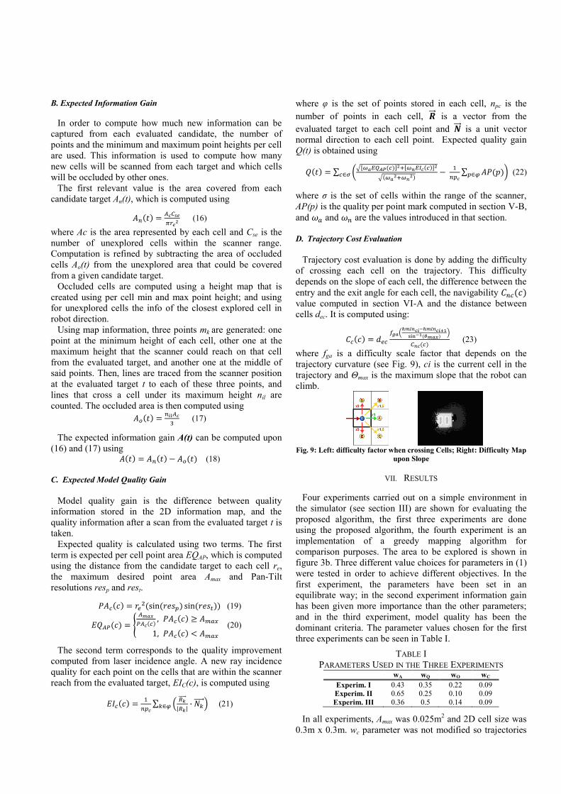
D. Trajectory Cost Evaluation

Trajectory cost evaluation is done by adding the difficulty

of crossing each cell on the trajectory. This difficulty

depends on the slope of each cell, the difference between the

entry and the exit angle for each cell, the navigability value computed in section VI-A and the distance between

cells dec. It is computed using:

(23)

where fga is a difficulty scale factor that depends on the

trajectory curvature (see Fig. 9), ci is the current cell in the

trajectory and Θmax is the maximum slope that the robot can

climb.

Fig. 9: Left: difficulty factor when crossing Cells; Right: Difficulty Map

upon Slope

VII. RESULTS

Four experiments carried out on a simple environment in

the simulator (see section III) are shown for evaluating the

proposed algorithm, the first three experiments are done

using the proposed algorithm, the fourth experiment is an

implementation of a greedy mapping algorithm for

comparison purposes. The area to be explored is shown in

figure 3b. Three different value choices for parameters in (1)

were tested in order to achieve different objectives. In the

first experiment, the parameters have been set in an

equilibrate way; in the second experiment information gain

has been given more importance than the other parameters;

and in the third experiment, model quality has been the

dominant criteria. The parameter values chosen for the first

three experiments can be seen in Table I.

TABLE I

PARAMETERS USED IN THE THREE EXPERIMENTS wA wQ wO wC

Experim. I 0.43 0.35 0.22 0.09

Experim. II 0.65 0.25 0.10 0.09

Experim. III 0.36 0.5 0.14 0.09

In all experiments, Amax was 0.025m2 and 2D cell size was

0.3m x 0.3m. wc parameter was not modified so trajectories

were determined only by the desired model criteria. The

amount of targets evaluated after each scan varies depending

on the number of traversable cells with a maximum of 1/25th

of those cells. Resulting trajectories can be seen in Fig. 10.

(a)

(b)

(c)

(d)

Fig. 10: Resulting trajectories for Exp. I (a); Exp. II (b); Exp. III (c);

Exp. IV(d). Colder Colours Represent Better Quality

Table II shows the result for each experiment in terms of

travelled distance, the number of scans done in each

experiment, the amount of cells explored within the given

area and a quality score given by the mean of per point

quality score on each cell within the area to be explored.

TABLE II

RESULTS OBTAINED IN EXPERIMENTS Travel

Distance

Quality

Score Coverage Scans

Experim. I 106 m 0.6846 92.5 % 12

Experim. II 107 m 0.6904 94.1 % 10

Experim. III 128 m 0.7503 93.6 % 13

Experim. IV 116 m 0.5013 91.4 % 8

All experiments were stopped when the coverage was over

90% of the reachable cells. Experiment II proved to be the

most efficient one since it covered the entire area using only

ten scans whilst travelling only 1 meter more than the

shortest trajectory. On the other hand, Experiment I provided

a very similar model but took two extra scans. Experiment

III required more scans (13) than any other test and more

travel distance than any other test; however it captured a

very high quality model.

Experiment IV showed that, in comparison with the greedy

mapping algorithm, the proposed algorithm may require

more scans to achieve the same level of coverage. However,

it leads to much higher quality score. The difference in terms

of traveled distance and coverage is not noticeable, but

trajectory is inefficient for greedy method since it requires

the robot to execute rougher turns for reaching the targets.

Finally, there is an important difference in the quality

distribution, this distribution being much more uniform in

the experiments carried out with the proposed algorithm, as

can be seen in Fig. 10.

Algorithm execution times vary greatly depending on the

amount of 3D data to be processed, however for these

experiments on a 3GHz Intel Core2 Duo processor the 3D

analysis process took around 350 ms each time a new scan

was made, and for the target evaluation step the evaluation

time for each target was at most 100 ms.

VIII. CONCLUSION

An algorithm for efficiently planning of viewpoints from

3D data, for 3D reconstruction of outdoor environments, has

been presented. Different criteria are used by this algorithm,

in order to obtain a model with quality over a predefined

minimum. The trajectory that the robot must follow in order

to reach each possible target is also considered, so the

process is carried out keeping a balance between the utility

of a point and the cost of getting to it.

The way the 3D data are processed in order to quantify the

model quality and extract navigation surfaces, obstacles and

interest regions has been discussed. Also a navigation map

useful for 3D environments and its resemblance to 2D

occupancy grid maps has been introduced.

The obtained results show that the algorithm can calculate

efficient trajectories for reconstructing the environment, and

that these trajectories change depending on the parameters

chosen to fulfill a given criterion. Also, our preliminary tests

of the algorithm implemented on the real robot (see Fig. 1)

have led to similar results than those obtained in simulation.

These results will be presented in future publications.

REFERENCES [1] P. Blaer and P. Allen, “Data Acquisition and View Planning for 3-D

Modeling Tasks”. In IROS2007, San Diego, 2007.

[2] A. Nuchter, K. Lingemann, and J. Hertzberg. “Extracting drivable surfaces in

outdoor 6d slam”. In the 37nd Symp. on Robotics (ISR ’06), Munich, 2006. [3] A. Nüchter, “3D Robotic Mapping”, Springer

[4] E. Bourque and G. Dudek, “Viewpoint selection-an autonomous robotic

system for virtual environment creation,” in IROS98, vol. 1, 1998,

[5] T. Danner and L. E. Kavraki, “Randomized Planning for Short Inspection

Paths,” Proceedings of IEEE International Conference on Robotics and

Automation ICRA '00. 2000.

[6] Tovey, C.; Koenig, S.; “Improved Analysis of Greedy Mapping”,

Proceedings of IEEE/RSJ International Conference on Intelligent Robots and Systems, (IROS 2003). 2003.

[7] B. Yamauchi, “A frontier-based approach for autonomous exploration,” in

Proceedings of the IEEE International Symposium on Computational

Intelligence in Robotics and Automation, July 1997, pp. 146–151.

[8] B. Yamauchi, A. Schultz, W. Adams, and K. Graves, “Integrating map

learning, localization and planning in a mobile robot,” in Intelligent Control

(ISIC), 1998. [9] P. Newman, M. Bosse, and J. Leonard, “Autonomous feature-based

exploration,” in the IEEE International Conference on Robotics and

Automation, 2003.

[10] H. H. Gonzalez-Baños and J. C. Latombe, “Navigation strategies for

exploring indoor environments.” International Journal of Robotics Research,

vol. 21, pp. 829–848, 2002.

[11] R. Grabowski, P. Khosla, and H. Choset. “Autonomous exploration via

regions of interest”. In IEEE IROS, pages 27–31, 2003. [12] K. Low and A. Lastra, "Efficient Constraint Evaluation Algorithms for

Hierarchical Next-Best-View Planning," Third International Symposium on

3D Data Processing, Visualization, and Transmission (3DPVT'06), 2006

[13] P. Blaer and P. Allen, “View Planning and Automated Data Acquisition for

Three-Dimensional Modeling of Complex Sites”, Journal of Field Robotics

26(11–12), 865–891 (2009)

[14] R. Smith; “Open Dynamics Engine”, http://www.ode.org/

[15] S. Rusinkiewicz, “trimesh2”, http://www.cs.princeton.edu/gfx/proj/trimesh2/ [16] R. Simmons, “Inter Process Communication”, http://www.cs.cmu.edu/~ipc/

[17] B. Gerkey and R. Vaughman; “The player project”,

http://playerstage.sourceforge.net/

[18] N. Basilico and F. Amigoni. “Exploration strategies based on multicriteria

decision making for an autonomous mobile robot”. Proc. ECMR09, 2009

[19] A. Nuchter, K. Lingemann, and J. Hertzberg. “Extracting drivable surfaces

in outdoor 6d slam”. In Proc. of the 37nd Int. Symp. on Robotics (ISR ’06), Munich, Germany, 2006.

[20] J. Hertzbert, K. Lingemann, C. Lorken, A. Nuchter and S. Stiene. “Does it

help a robot navigate to call navigability an affordance?”. Towards

affordance-based robot control. In Lecture Notes in Computer Science 2008.