algorithm engineering in robust optimization - arxiv · algorithm engineering in robust...
TRANSCRIPT

Algorithm Engineering in RobustOptimization∗
Marc Goerigk†1 and Anita Schobel‡2
1University of Kaiserslautern, Germany2University of Gottingen, Germany
Abstract
Robust optimization is a young and emerging field of research having receiveda considerable increase of interest over the last decade. In this paper, we arguethat the the algorithm engineering methodology fits very well to the field of robustoptimization and yields a rewarding new perspective on both the current state ofresearch and open research directions.
To this end we go through the algorithm engineering cycle of design and analysisof concepts, development and implementation of algorithms, and theoretical andexperimental evaluation. We show that many ideas of algorithm engineering havealready been applied in publications on robust optimization. Most work on robustoptimization is devoted to analysis of the concepts and the development of algo-rithms, some papers deal with the evaluation of a particular concept in case studies,and work on comparison of concepts just starts. What is still a drawback in manypapers on robustness is the missing link to include the results of the experimentsagain in the design.
1 Introduction
Similar to the approach of stochastic optimization, robust optimization deals with mod-els in which the exact data is unknown, but bounded by a set of possible realizations(or scenarios). Contrary to the former approach, in robust optimization, one typicallyrefrains from assuming a given probability distribution over the scenarios. While thefirst steps in robust optimization trace back to the work of Soyster [Soy73], it has notemerged as a field of research in its own right before the late 90s with the seminal worksof Ben-Tal, Nemirovski, and co-authors (see [BTN98,BTN99], and many more).
∗Partially supported by grant SCHO 1140/3-2 within the DFG programme Algorithm Engineering andby FP7-PEOPLE-2009-IRSES under the OptALI grant agreement no 246647.
†Email: [email protected]‡Email: [email protected]
1
arX
iv:1
505.
0490
1v3
[m
ath.
OC
] 1
1 Ja
n 20
16

In this section, we first describe the general setting of robust optimization in moredetail, and then discuss the algorithm engineering methodology and its application,which gives a natural structure for the remainder of the paper.
Uncertain optimization problems. Nearly every optimization problem suffers from un-certainty to some degree, even if this does not seem to be the case at first sight. Generallyspeaking, we may distinguish two types of uncertainty: Microscopic uncertainty, such asnumerical errors and measurement errors; and macroscopic uncertainty, such as forecasterrors, disturbances or other conditions changing the environment where a solution isimplemented.
In “classic” optimization, one would define a so-called nominal scenario, which de-scribes the expected or “most typical” behavior of the uncertain data. Depending onthe uncertainty type, this scenario may be, e.g., the coefficient of the given precision fornumerical errors, the measured value for measurement errors, the most likely forecastfor forecast errors, or an average environment for long-term solutions. Depending on theapplication, computing such a scenario may be a non-trivial process, see, e.g., [Jen00].
In this paper we consider optimization problems that can be written in the form
(P ) min f(x)
s.t. F (x) ≤ 0
x ∈ X ,
where F : Rn → Rm describes the m problem constraints, f : Rn → R is the objectivefunction, and X ⊆ Rn is the variable space. In real-world applications, both the con-straints and the objective may depend on parameters which are uncertain. In order toaccommodate such uncertainties, instead of (P ), the following parameterized family ofproblems is considered:
(P (ξ)) min f(x, ξ)
s.t. F (x, ξ) ≤ 0
x ∈ X ,
where F (·, ξ) : Rn → Rm and f(·, ξ) : Rn → R for any fixed ξ ∈ RM . Every ξ describesa scenario that may occur.
Although it is in practice often not known exactly which values such a scenario ξ maytake for an optimization problem P (ξ), we assume that it is known that ξ lies within agiven uncertainty set U ⊆ RM . Such an uncertainty set represents the scenarios whichare likely enough to be considered.
The uncertain optimization problem corresponding to P (ξ) is then denoted as
(P (ξ), ξ ∈ U) . (1)
Note that the uncertain optimization problem in fact consists of a whole set of parame-terized problems, that is often even infinitely large. The purpose of robust optimization
2

concepts is to transform this family of problems back into a single problem, which iscalled the robust counterpart. The choice of the uncertainty set is of major impact notonly for the respective application, but also for the computational complexity of theresulting robust counterpart. It hence has to be chosen carefully by the modeler.
For a given uncertain optimization problem (P (ξ), ξ ∈ U), we denote by
F(ξ) = x ∈ X : F (x, ξ) ≤ 0
the feasible set of scenario ξ ∈ U . Furthermore, if there exists a nominal scenario, it isdenoted by ξ ∈ U . The optimal objective value for a single scenario ξ ∈ U is denoted byf∗(ξ).
We say that an uncertain optimization problem (P (ξ), ξ ∈ U) has convex (quasiconvex,affine, linear) uncertainty, when both functions, F (x, ·) : U → Rm and f(x, ·) : U → Rare convex (quasiconvex, affine, linear) in ξ for every fixed x ∈ X .
Common uncertainty sets. There are some types of uncertainty sets that are frequentlyused in current literature. These include:
1. Finite uncertainty U =ξ1, . . . , ξN
2. Interval-based uncertainty U = [ξ
1, ξ1]× . . .× [ξ
M, ξM ]
3. Polytopic uncertainty U = convξ1, . . . , ξN
4. Norm-based uncertainty U =
ξ ∈ RM : ‖ξ − ξ‖ ≤ α
for some parameter α ≥ 0
5. Ellipsoidal uncertainty U =
ξ ∈ RM :
√∑Mi=1 ξ
2i /σ
2i ≤ Ω
for some parameter
Ω ≥ 0
6. Constraint-wise uncertainty U = U1 × . . .× Um, where Ui only affects constraint i
where convξ1, . . . , ξN
=∑N
i=1 λiξi :∑N
i=1 λi = 1, λ ∈ RN+
denotes the convex hull
of a set of points. Note that this classification is not exclusive, i.e., a given uncertaintyset can belong to multiple types at the same time.
The algorithm engineering methodology, and the structure of this paper. In thealgorithm engineering approach, a feedback cycle between design, analysis, implementa-tions, and experiments is used (see [San09] for a detailed discussion). We reproduce thiscycle for robust optimization in Figure 1.
While this approach usually focuses on the design and analysis of algorithms, oneneeds to consider the important role that different concepts play in robust optimization.Moreover, as is also discussed later, there is a thin line between what is to be considereda robustness concept, and an algorithm – e.g., the usage of a simplified model for a ro-bustness concept could be considered as a new concept, but also as a heuristic algorithm
3

applications with uncertain data
performanceguarantees
experiments
implementation
realinputs
designof concepts and algorithms
analysisof concepts and algorithms
libraries ofalgorithms
and concepts
realisticmodels and
uncertainty sets
Figure 1: The algorithm engineering cycle for robust optimization following [San09].
4

for the original concept. We will therefore consider the design and analysis of both,concepts and algorithms.
The algorithm engineering approach has been successfully applied to many problemsand often achieved impressive speed-ups (as in routing algorithms, see, e.g. [DSSW09]and the book [MHS10]).
Even though this aspect has not been sufficiently acknowledged in the robust opti-mization community, the algorithm engineering paradigm fits very well in the line ofresearch done in this area: In algorithm engineering it is of particular importance thatthe single steps in the depicted cycle are not considered individually, but that specialstructure occurring in typical instances is identified and used in the development andanalysis of concepts and algorithms. As we will show in the following sections theselinks to real-world applications and to the structure of the uncertain data are of specialimportance in particular in robust optimization. Various applications with different un-derstandings of what defines a robust solution triggered the development of the differentrobustness concepts (see Section 2) while the particular structure of the uncertainty setled to adapted algorithms (see Section 3.1).
Moreover, the algorithm engineering cycle is well-suited to detect the missing researchlinks to push the developed methods further into practice. A key aspect of this paperhence is to draw further attention to the potential of algorithm engineering for robustoptimization.
We structure the paper along the algorithm engineering cycle, where we discuss eachstep separately, providing a few exemplarily papers dealing with the respective matters.Missing links to trigger further research in this areas are pointed out. Specifically, weconsider
• design of robustness concepts in Section 2,
• analysis of robustness concepts in Section 3,
• design and analysis of algorithms in Section 4, and
• implementations and experiments in Section 5.
Applications of robust optimization are various, and strongly influenced the design ofrobustness concepts while the design of algorithms was rather driven by an analysis ofthe respective uncertainty sets. Some of these relations are mentioned in the respectivesections. The paper is concluded in Section 6 where we also demonstrate on someexamples how the previously mentioned results can be interpreted in the light of thealgorithm engineering methodology.
2 Design of Robustness Concepts
Robust optimization started with rather conservative concepts hedging against every-thing that is considered as being likely enough to happen. Driven by various othersituations and applications calling for “robust” solutions these concepts were further
5

developed. In this section we give an overview on the most important older and somerecent concepts. We put special emphasis on the impact applications with uncertaindata have on the design of robustness concepts (as depicted in in Figure 1), and howreal-world requirements influence the development of robustness models.
2.1 Strict Robustness
This approach, which is sometimes also known as classic robust optimization, one-stagerobustness, min-max optimization, absolute deviation, or simply robust optimization,can be seen as the pivotal starting point in the field of robustness. A solution x ∈ Xto the uncertain problem (P (ξ), ξ ∈ U) is called strictly robust if it is feasible for allscenarios in U , i.e. if F (x, ξ) ≤ 0 for all ξ ∈ U . The objective usually follows thepessimistic view of minimizing the worst-case over all scenarios. Denoting the set ofstrictly robust solutions with respect to the uncertainty set U by
SR(U) =⋂ξ∈UF(ξ),
the strictly robust counterpart of the uncertain optimization problem is given as
(SR) min supξ∈U
f(x, ξ)
s.t. x ∈ SR(U)
x ∈ X .
The first to consider this type of problems from the perspective of generalized linearprograms was Soyster [Soy73] for uncertainty sets U of type
U = K1 × . . .×Kn,
where the set Ki contains possible column vectors Ai of the coefficient matrix A.Subsequent works on this topic include [Fal76] and [Thu80].
However, building this approach into a strong theoretic framework is due to a seriesof papers by Ben-Tal, Nemirovski, El Ghaoui and co-workers [GL97, BTN98, BTN99,BTN00]. A summary of their results can be found in the book [BTGN09]. Their basicunderlying idea is to hedge against all scenarios that may occur. As they argue, such anapproach makes sense in many settings, e.g., when constructing a bridge which must bestable, no matter which traffic scenario occurs, or for airplanes or nuclear power plants.However, this high degree of conservatism of strict robustness is not applicable to allsituations which call for robust solutions. An example for this is timetabling in publictransportation: being strictly robust for a timetable means that all announced arrivaland departure times have to be met, no matter what happens. This may mean to addhigh buffer times, depending on the uncertainty set used, and thus would not resultin a practically applicable timetable. Such applications triggered research in robustoptimization on ways to relax the concept. We now describe some of these approaches.
6

2.2 Cardinality Constrained Robustness
One possibility to overcome the conservatism of strict robustness is to shrink the uncer-tainty set U . This has been conceptually introduced by Bertsimas and Sim in [BS04] forlinear programming problems. Due to this reason, this concept is sometimes also knownas “the approach of Bertsimas and Sim”, sometimes also under the name “Γ-robustness”.Analyzing the structure of uncertainty sets in typical applications, they observed that itis unlikely that all coefficients of one constraint change simultaneously to their worst-casevalues. Instead they propose to hedge only against scenarios in which at most Γ uncer-tain parameters per constraint change to their worst-case values, i.e., they restrict thenumber of coefficients which are allowed to change leading to the concept of cardinalityconstrained robustness. Considering a constraint of the form
a1x1 + . . .+ anxn ≤ b
with an uncertainty U = a ∈ Rn : ai ∈ [ai − di, ai + di], i = 1, . . . , n, their robustnessconcept requires a solution x to satisfy
n∑i=1
aixi + maxS⊆1,...,n,|S|=Γ
∑i∈S
di|xi|
≤ b
for a given parameter Γ ∈ 0, . . . , n. Any solution x to this model hence hedges againstall scenarios in which at most Γ many uncertain coefficients may deviate from theirnominal values at the same time.
It can be shown that cardinality constrained robustness can also be considered asstrict robustness using the convex hull of the cardinality-constrained uncertainty set
U(Γ) = a ∈ U : ai 6= ai for at most Γ indices i ⊆ U .
Since conv(U(Γ)) is a polyhedral set, results on strict robustness with respect topolyhedral uncertainty can also be applied to cardinality constrained robustness.
Note that this approach also extends to fractional values of Γ. Their concept hasbeen extended to uncertainty sets under general norms in [BPS04]. The approach tocombinatorial optimization problems has been generalized in [Ata06] and [GST12].
2.3 Adjustable Robustness
In [BTGGN03] a completely different observation of instances occurring in real-worldproblems with uncertain data is used: Often the variables can be decomposed intotwo sets. The values for the here-and-now variables have to be found by the robustoptimization algorithm in advance, while the decision about the wait-and-see variablescan wait until the actual scenario ξ ∈ U becomes known. Note that this is similar totwo-stage programming in stochastic optimization.
We therefore assume that the variables x = (u, v) are splitted into u ∈ X 1 ⊆ Rn1 andv ∈ X 2 ⊆ Rn2 with n1 + n2 = n, where the variables u need to be determined before
7

the scenario ξ ∈ U becomes known, while the variables v may be determined after ξ hasbeen realized. Thus, we may also write x(ξ) to emphasize the dependence of v on thescenarios. The uncertain optimization problem (P (ξ), ξ ∈ U) is rewritten as
P (ξ) min f(u, v, ξ)
F (u, v, ξ) ≤ 0
(u, v) ∈ X 1 ×X 2.
When fixing the here-and-now variables, one has to make sure that for any possiblescenario ξ ∈ U there exists v ∈ X 2 such that (u, v) is feasible for ξ. The set of adjustablerobust solutions is therefore given by
aSR = u ∈ X 1 : ∀ξ ∈ U ∃v ∈ X 2 s.t. (u, v) ∈ F(ξ)
=⋂ξ∈U
PrX 1(F(ξ)),
where PrX 1(F(ξ)) = u ∈ X 1 : ∃v ∈ X 2 s.t. (u, v) ∈ F(ξ) denotes the projection ofF(ξ) on X 1.
The worst case objective for some u ∈ aSR is given as
zaSR(u) = supξ∈U
infv:(u,v)∈F(ξ)
f(u, v, ξ).
The adjustable robust counterpart is then given as
minzaSR(u) : u ∈ aSR.
Note that this setting is also useful for another type of problem instances, namely, ifauxiliary variables are used that do not represent decisions, e.g., additional variables tomodel the absolute value of a variable.
There are several variations of the concept of adjustable robustness. Instead of twostages, multiple stages are possible. In the approach of finitely adaptable solutions[BC10], instead of computing a new solution for each scenario, a set of possible staticsolutions is computed, such that at least one of them is feasible in each stage.
Furthermore, the development of adjustable robustness was preceded by the similarapproach of Mulvey et al [MVZ95]. They considered an uncertain linear optimizationproblem of the form
(P(B,C, e)) min ctu+ dtv
s.t. Au = b
Bu+ Cv = e
u ∈ Rn1+ , v ∈ Rn2
+ ,
where u represents a vector of design variables that cannot be adjusted, and v a vectorof control variables that can be adjusted when the realized scenario becomes known. For
8

a finite uncertainty set U = (B1, C1, e1), . . . , (BN , CN , eN ), their robust counterpartis given as
(Mul) min σ(u, v1, . . . , vN ) + ωρ(z1, . . . , zN )
s.t. Au = b
Biu+ Civi + zi = ei ∀i = 1, . . . , N
u ∈ Rn1+ , vi ∈ Rn2
+ , zi ∈ Rm.
The variables zi are introduced to measure the infeasibility in every scenario, i.e., thedeviation from the right-hand side. The function σ represents the solution robustness.It can be modeled as a worst-case function of the nominal objective
σ(u, v1, . . . , vN ) = ctu+ maxi=1,...,N
dtvi
or, when probabilities pi are known, as an expected nominal objective. The function ρon the other hand represents the model robustness and depends on the infeasibility ofthe uncertain constraints. Possible penalty functions are
ρ(z1, . . . , zN ) =N∑i=1
pi
m∑j=1
max0, zij
or =
N∑i=1
pi(zi)tzi.
As (Mul) is actually a bicriteria model, ω is used as a scalarization factor to combineboth objectives.
2.4 Light Robustness
The lightly robust counterpart of an uncertain optimization problem, as developed in[FM09] and generalized in [Sch14] is again application driven. Originally developedfor timetabling, the idea of light robustness is that a solution must not be too bad inthe nominal case. For example, the printed timetable should have short travel timesif everything runs smoothly and without disturbances; or a planned schedule shouldhave a small makespan. In this sense a certain nominal quality is fixed. Among allsolutions satisfying this standard, the concept asks for the most “reliable” one withrespect to constraint violation. Specifically, the general lightly robust counterpart asdefined in [Sch14] is of the following form:
(LR) min
m∑i=1
wiγi
s.t. f(x, ξ) ≤ f∗(ξ) + ρ
F (x, ξ) ≤ γ ∀ξ ∈ Ux ∈ X , γ ∈ Rm,
9

where wi models a penalty weight for the violation of constraint i and ρ determines therequired nominal quality. We denote by ξ the nominal scenario, as introduced on page 3.This approach was in its first application in [FM09] used as a further development ofthe concept of cardinality constrained robustness (see Section 2.2).
Note that a constraint of the form F (x, ξ) ≤ 0 is equivalent to a constraint λF (x, ξ) ≤ 0for any λ > 0; therefore, the coefficients wi play an important role in balancing theallowed violation of the given constraints.
2.5 Recoverable Robustness
Similar to adjustable robustness, recoverable robustness is again a two-stage concept.It has been developed in [CDS+07, Sti08, LLMS09, DDN09] and has independently alsobeen used in [EMS09]. Its basic idea is to allow a class of recovery algorithms A thatcan be used in case of a disturbance. A solution x is called recovery robust with respectto A if for any possible scenario ξ ∈ U there exists an algorithm A ∈ A such that Aapplied to the solution x and the scenario ξ constructs a solution A(x, ξ) ∈ F(ξ), i.e., asolution which is feasible for the current scenario.
The recovery robust counterpart according to [LLMS09] is the following:
(RR) min(x,A)∈F(ξ)×A
f(x)
s.t. A(x, ξ) ∈ F(ξ) ∀ξ ∈ U .
It can be extended by including the recovery costs of a solution x: Let d(A(x, ξ)) be apossible vector-valued function that measures the costs of the recovery, and let λ ∈ Λbe a limit on the recovery costs, i.e., λ ≥ d(A(x, ξ)) for all ξ ∈ U . Assume that there issome cost function g : Λ→ R associated with λ.
SettingA(x, ξ, λ) ∈ F ′(ξ) ⇐⇒ d(A(x, ξ)) ≤ λ ∧ A(x, ξ) ∈ F(ξ)
gives the recovery robust counterpart with limited recovery costs:
(RR-LIM) min(x,A,λ)∈F(ξ)×A×Λ
f(x) + g(λ)
s.t. A(x, ξ, λ) ∈ F ′(ξ) ∀ξ ∈ U .
Due to the generality of this robustness concept, the computational tractability heav-ily depends on the problem, the recovery algorithms and the uncertainty under con-sideration. In [GS10, GS11a, Goe12, GS14], the concept of recoverable robustness hasbeen considered under the usage of metrics to measure recovery costs. The aim is tominimize the costs when recovering, where they differ between recovering to a feasiblesolution (“recovery-to-feasibility”), and recovering to an optimal solution (“recovery-to-optimality”) in the realized scenario.
10

2.6 Regret Robustness
The concept of regret robustness differs from the other presented robustness conceptsinsofar it usually only considers uncertainty in the objective function. Instead of min-imizing the worst-case performance of a solution, it minimizes the difference to theobjective function of the best solution that would have been possible in a scenario. Insome publications, it is also called deviation robustness.
Let f∗(ξ) denote the best objective value in scenario ξ ∈ U . The min-max regretcounterpart of an uncertain optimization problem with uncertainty in the objective isthen given by
(Regret) min supξ∈U
(f(x, ξ)− f∗(ξ)
)s.t. F (x) ≤ 0
x ∈ X .
Regret robustness is a concept with a vast amount of applications, e.g., in location theoryor in scheduling. For a survey on this concept, see [ABV09] and [KY97]. In a similarspirit, the concept of lexicographic α-robustness has been recently proposed [KLV12].Its basic idea is to evaluate a fixed solution by reordering the set of scenarios accordingto the performance of the solution. This performance curve is then compared to an idealcurve, where the optimization problem is solved separately for every scenario.
2.7 Some Further Robustness Concepts
Reliability. Another approach to robust optimization is to relax the constraints of strictrobustness. This leads to the concept of reliability of Ben-Tal and Nemirovski [BTN00],in which the constraints F (x, ξ) ≤ 0 are replaced by F (x, ξ) ≤ γ for some γ ∈ Rm≥0. Asolution x which satisfies
F (x, ξ) ≤ γ for all ξ ∈ Uis called reliable with respect to γ. The goal is to find a reliable solution which minimizesthe original objective function in the worst case. Similar to light robustness, one hasto be careful that the representation of the constraints does not affect the reliability ofthe solution, otherwise one may obtain the counter-intuitive result that, although theconstraints F (x, ξ) ≤ 0 can also be written as Ψ(F (x, ξ)) ≤ 0 for any increasing Ψ withΨ(0) = 0, what is understood by a robust solution may be different if one models theconstraints with F or with Ψ(F ).
Soft Robustness. The basic idea of soft robustness as introduced in [BTBB10] is tohandle the conservatism of the strict robust approach by considering a nested family ofuncertainty sets, and allowing more deviation in the constraints for larger uncertainties.Specifically, instead of an uncertainty set U ⊆ RM , a family of uncertainties U(ε) ⊆Uε>0 with U(ε1) ⊆ U(ε2) for all ε2 ≥ ε1 is used. The set of soft robust solutions is thengiven as
softR = x ∈ X : F (x, ξ) ≤ ε ∀ξ ∈ U(ε), ε > 0 .
11

Note that strict robustness is a special case with U(ε) = U for all ε > 0.In [BTBB10], the authors show that a solution to the softly robust counterpart –
i.e., the optimization over softR with a worst-case objective – can be found by solving asequence of strictly robust counterparts using a bisection approach over ε, and analyzethe numerical performance on a bond portfolio and an asset allocation problem.
Comprehensive Robustness. While the adjustable robust approach relaxes the as-sumption that all decisions have to be made before the realized scenario becomes known,the approach of comprehensively robust counterparts [BTBN06] also removes the as-sumption that only scenarios defined in the uncertainty set U need to be considered.Instead, using a distance measure dist in the space of scenarios, and a distance measuredist in the solution space, they assume that the further away a scenario is from the un-certainty set, the further away the corresponding solution is allowed to be from the setof feasible solutions. As in adjustable robustness, the dependence of x on the scenarioξ is allowed, and we may write x(ξ). The adjustable robust counterpart is extended tothe following problem:
(CRC) min z
s.t. f(x(ξ), ξ) ≤ z + α0dist(ξ,U) ∀ξdist(x(ξ),F(ξ)) ≤ αdist(ξ,U) ∀ξ,
where α, α0 denote sensitivity parameters. This formulation needs further formal speci-fication, which is provided in [BTBN06].
Uncertainty Feature Optimization. Instead of assuming that an explicit uncertaintyset is given, which may be hard to model for real-world problems, the uncertainty featureoptimization (UFO) approach [ESB11] rather assumes that the robustness of a solutionis given by an explicit function. For an uncertain optimization problem (P (ξ)), letµ : Rn → Rp be a measure for p robustness features. The UFO-counterpart of theuncertain problem is then given by
(UFO) vecmax µ(x)
s.t. F (x) ≤ 0
f(x) ≤ (1 + ρ)f∗(ξ)
x ∈ X ,
where f∗(ξ) denotes the best objective value to the nominal problem. The authorsshow that this approach generalizes both stochastic optimization and the concept ofcardinality constrained robustness of Bertsimas and Sim.
2.8 Summary
As this section shows, we cannot actually speak of one concept or point-of-view to be“robust optimization”; instead, we should see it as a vast collection of different robust-ness concepts, each providing their unique advantages and disadvantages. Generally
12

speaking, there is usually a trade-off between the degree of freedom a concept givesto react to disruptions (including what is considered as being a disruption, i.e., thechoice of the uncertainty set), and its computational complexity. From an algorithmengineering point of view, the size of this “toolbox” of different concepts significantlyhelps with finding a suitable robustness concept for a given problem. However, as theseconcepts are usually application-driven, they lack a generalizing systematics: Appli-cations tend to develop “their own approach” to robustness instead of making use ofthe existing body of literature, and develop their own notation and names along theway. In fact, the very same concepts are known under plenty of names. Summariesas [BTGN09,ABV09,BBC11,Roy10] usually avoid this Babylonian “zoo” of robustnessconcepts and nomenclature by focusing only on the mainstream concepts. Thus, wesuggest the following pointer to further research:
Remark 1 Robust optimization needs a unified classification scheme.
3 Analysis of Robustness Concepts
Not only the development of robustness concepts, but also their analysis is data-driven.This becomes in particular clear when looking at the structure of the underlying uncer-tainty set. A large amount of research in the analysis of robustness concepts is devotedto finding equivalent problem formulations that are better tractable, using the structureof the uncertainty set.
In this section we first review this line of research, and then briefly point out exem-plarily which other types of structure or ideas have been used in the analysis of concepts.
3.1 Using the structure of the uncertainty set
Finite uncertainty set. If the uncertainty set U = ξ1, . . . , ξN is a finite set containingnot too many scenarios, most of the robustness concepts can be formulated as mathe-matical programs by just adding the constraints for each of the scenarios explicitly. Thiscan straightforwardly been done for strict robustness yielding
(SR) min z
s.t. f(x, ξi) ≤ z for i = 1, . . . , N
s.t. F (x, ξi) ≤ 0 for i = 1, . . . , N
x ∈ X .
as the strictly robust counterpart. Reliability and light robustness can be treated anal-ogously. In all three cases, the robust counterpart keeps many properties of the original(non-robust) problem formulation: If the original formulation was e.g., a linear program,also its robust counterpart is. The same holds for differentiability, convexity, and manyother properties.
For regret robustness one needs to precompute the best objective function value foreach scenario ξ1, i = 1, . . . , N in order to receive again a straightforward reformulation.
13

Also in adjustable and recoverable robustness mathematical programming formulationscan be derived by adding a wait and see variable, or a group of recovery variables foreach of the scenarios. This usually leads to a high number of additional variables but is(at least for linear programming) often still solvable.
Note that the concept of cardinality constrained robustness does not make much sensefor a finite set of scenarios since it concerns the restriction which scenarios might oc-cur. For a finite set, scenarios in which too many parameters change can be removedbeforehand.
Polytopic uncertainty. Let f(x, ·) and F (x, ·) be quasiconvex in ξ for any fixed x ∈ X .Then there are robustness concepts in which the following reduction result holds: Therobust counterpart w.r.t. an uncertainty set U ′ is equivalent to the robust counterpartw.r.t. U := conv(U ′). In such cases the robust counterpart w.r.t. a polytopic uncer-tainty set U = convξ1, . . . , ξN is equivalent to the robust counterpart w.r.t. the finiteuncertainty set ξ1, . . . , ξN, hence the formulations for finite uncertainty sets can beused to treat polytopic uncertainties.
We now review for which robustness concepts the reduction result holds. First of all,this is true for strict robustness, For affine and convex uncertainty this was mentionedin [BTN98]; the generalization to quasiconvex uncertainty is straightforward. One of thedirect consequences, namely that the robust counterpart of an uncertain linear programunder these conditions is again a linear program was mentioned in [BTN00]. The sameresult holds for reliability since the reliable robust counterpart can be transformed to astrictly convex counterpart by defining F (x, ξ) = F (x, ξ)− γ. For light robustness, theresult is also true, see [Sch14]. For the case of adjustable robustness, [BTGGN03] showedthat the result holds for problems with fixed recourse. Otherwise, counterexamples canbe constructed. The generalization to nonlinear two-stage problems and quasiconvexuncertainty is due to [TTT08]. For recoverable robustness there exist special cases inwhich the recovery robust counterpart is equivalent to an adjustable robust counterpartwith fixed recourse. In these cases, the result of [BTGGN03] may be applied. However,in general, recoverable robustness does not allow this property. This also holds forrecovery-to-optimality.
Interval-based uncertainty. Interval-based uncertainty can be interpreted as a specialcase of polytopic uncertainty where the polytope is a box U = [ξ
1, ξ1] × . . . × [ξ
M, ξM ]
with 2M extreme points (ξ1, ξ2, . . . , ξM )t ∈ RM , where ξi ∈ ξi, ξi, i = 1, . . . ,M . Hence,all the results for polytopic uncertainty apply. They can often be simplified by observingthat not all extreme points are needed since the respective constraints often dominateeach other, yielding a drastic speed-up when solving the robust counterpart.
For their concept of cardinality constrained robustness, Bertsimas and Sim [BS04]considered interval-based uncertainty sets for linear programs. This can be interpreted asstrict robustness with a new uncertainty set U ′ only allowing scenarios in which not morethan Γ uncertain parameters per constraint change their values (see also [BPS04]). Thisuncertainty set U ′ is a polytope, hence the robust counterpart for cardinality constrained
14

robustness stays a linear program for interval-based uncertainty.
Ellipsoidal uncertainty. The case of ellipsoidal uncertainty is studied extensively forstrict robustness and for adjustable robustness in [BTGN09]. It could be shown thatoften the constraint
F (x, ξ) ≤ 0 for all ξ ∈ U
can be replaced by a finite number of constraints for ellipsoidal uncertainty sets. How-ever, it has been shown in [BTGN09] that for ellipsoidal uncertainty, the structure ofthe strictly robust counterpart gets more complicated. For example (see [BTN98]) thestrictly robust counterpart of a linear program is a conic quadratic program, the strictlyrobust counterpart of a quadratic constrained quadratic program is a semidefinite pro-gram, the strictly robust counterpart of a second order cone program is a semidefiniteprogram, and the strictly robust counterpart of a semidefinite program is NP-hard. Asmentioned before, all these results can be transferred to reliability.
For light robustness, it has been shown in [Sch14] that the lightly robust counterpart ofa linear program with ellipsoidal uncertainty becomes a quadratic program. Ellipsoidaluncertainty could receive more attention also for other robustness concepts (e.g., forregret robustness, which usually only considers finite or interval-based uncertainty, see[ABV09]), or for adjustable robustness, see [BTGN09].
3.2 Using duality
Duality in uncertain programs has been considered as early as 1980, see [Thu80]. In[BBT09], it is shown that “the primal worst equals the dual best”, i.e., under quite gen-eral constraints, the dual of a strictly robust counterpart (a min-max problem) amountsto optimization under the best case instead of the worst-case (a max-min problem). Sincethen, duality in robust optimization has been a vivid field of research, see, e.g., [JLS13]and [SKL13]. In the following, we highlight two applications of duality for robust opti-mization: One for constraints, and one for objectives.
Duality in the constraints.
Duality is a useful tool for the reformulation of robust constraints. We exemplarilydemonstrate this using two applications.
In [BS04], the authors show that the cardinality constrained robust counterpart canbe linearized by using the dual of the inner maximization problem. This yields
n∑i=1
aixi + zΓ +
n∑i=1
pi ≤ b
z + pi ≥ diyi ∀i = 1, . . . , n
− yi ≤ xi ≤ yi ∀i = 1, . . . , n
p, y, z ≥ 0.
15

Note that a general, robust constraint of the form
f(x, ξ) ≤ 0 ∀ξ ∈ U
can be rewritten asmaxξ∈U
f(x, ξ) ≤ 0.
This is used in [BTdHV14]. With a concave function f(x, ·) and an uncertainty setU = ξ + Aζ : ζ ∈ Z with a nonempty, convex and compact set Z, applying dualityyields
ξtv + δ∗(AT v|Z)− f∗(v, x) ≤ 0
where δ∗ is the support function, f∗ is a conjugate function, and other technical require-ments are met. This gives a very general tool to compute robust counterparts; e.g.,a linear constraint of the form f(x, ξ) = ξtx − β and Z = ζ : ‖ζ‖2 ≤ ρ yields thecounterpart ξtx+ ρ‖Atx‖2 ≤ β.
Duality in the objective.
In many papers, duality is used to change the typical min-max objective of a robustcounterpart into a min min objective by using the dual formulation of the inner maxi-mization problem.
This method was first applied to the spanning tree problem [YKP01], and later ex-tended to the general case of optimization problems with zero duality gap in [ABV09].Let an uncertain optimization problem of the form
min ctx
s.t. x ∈ X = x ∈ 0, 1n : Ax ≥ b
with interval-based uncertainty in c be given; i.e., ci ∈ [ci, ci]. Then we may write
minx∈X
maxc∈U
(f(x, c)− f∗(c))
= minx∈X
maxc∈U ,y∈X
(ctx− cty
)= min
x∈X
(cx−min
y∈Xcwc(x)y
),
where cwc(x) denotes the regret worst-case for x, given as ci if xi = 1, and ci if xi = 0.Using that the duality gap is zero, we can insert the dual to the inner optimizationproblem, and get the following equivalent problem:
min cx− btys.t. Ax ≥ b
Aty ≤ (c− c)x+ c
x ∈ 0, 1n, y ∈ Rn+
This reformulation can then be solved using, e.g., a branch and bound approach.
16
4 Design and Analysis of Algorithms
Concerning the design and analysis of algorithms we concentrate on the most matureconcept, namely on algorithms for strict robustness. Many approaches, often based onsimilar ideas, also exist for regret optimization – e.g., cutting plane approaches [IS95,ML99, ML98], or preprocessing considerations [YKP01, KZ10]. For the other concepts,approaches are currently still being developed.
The robust counterpart per se is a semi-infinite program; thus, all methods that applyto semi-infinite programming [LS07] can be used here as well. However, the special min-max structure of the robust counterpart allows improved algorithms over the generalcase, in particular for the reformulations based on special uncertainty sets as mentionedin Section 3.1.
In the following, we discuss algorithms that are generically applicable to strictly robustoptimization problems.
4.1 Finite Scenarios
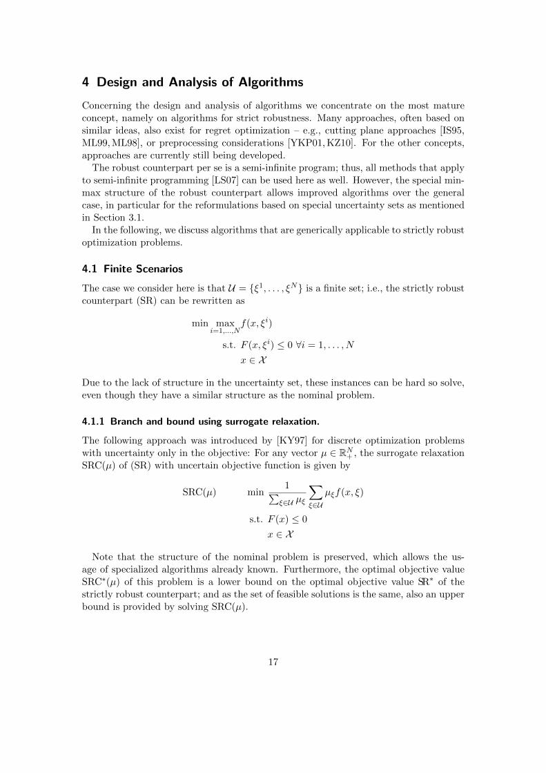
The case we consider here is that U = ξ1, . . . , ξN is a finite set; i.e., the strictly robustcounterpart (SR) can be rewritten as
min maxi=1,...,N
f(x, ξi)
s.t. F (x, ξi) ≤ 0 ∀i = 1, . . . , N
x ∈ X
Due to the lack of structure in the uncertainty set, these instances can be hard so solve,even though they have a similar structure as the nominal problem.
4.1.1 Branch and bound using surrogate relaxation.
The following approach was introduced by [KY97] for discrete optimization problemswith uncertainty only in the objective: For any vector µ ∈ RN+ , the surrogate relaxationSRC(µ) of (SR) with uncertain objective function is given by
SRC(µ) min1∑
ξ∈U µξ
∑ξ∈U
µξf(x, ξ)
s.t. F (x) ≤ 0
x ∈ X
Note that the structure of the nominal problem is preserved, which allows the us-age of specialized algorithms already known. Furthermore, the optimal objective valueSRC∗(µ) of this problem is a lower bound on the optimal objective value SR∗ of thestrictly robust counterpart; and as the set of feasible solutions is the same, also an upperbound is provided by solving SRC(µ).
17

This approach is further extended by solving the problem
maxµ∈RN
+
SRC∗(µ),
i.e., by finding the multiplier µ that yields the strongest lower bound. This can be doneusing a sub-gradient method.
The lower and upper bounds generated by the surrogate relaxation are then usedwithin a branch and bound framework on the x variables. The approach was furtherimproved for the knapsack problem in [Iid99,TYK08].
4.1.2 Local search heuristics.
In [Sbi10], a local search-based algorithm for the knapsack problem with uncertain objec-tive function is developed. We briefly list the main aspects. It makes use of two differentsearch procedures: Given a feasible solution x and a list of local neighborhood movesM , let GS(x,M) (the generalized search) determine the worst-case objective value ofevery move, and return the best move along with its objective value. Furthermore, letRS(x,M, S) (the restricted search) perform a random search using the moves M withat most S steps.
The cooperative local search algorithm (CLS) works as follows: It first constructs aheuristic starting solution, e.g., by a greedy approach. In every iteration, a set of movesM is constructed using either the generalized search for sets with small cardinality, or therestricted search for sets with large cardinality. When a maximum number of iterationsis reached, the best feasible solution found so far is returned.
4.1.3 Approximation algorithms.
A discussion of approximation algorithms for strict robustness with finitely many scenar-ios is given, e.g., in [ABV07], where it is shown that there is an FPTAS for the shortestpath, the spanning tree, and the knapsack problem when the number of scenarios isconstant; but the shortest path problem is not (2− ε)-approximable, the spanning treeproblem is not (3
2 − ε)-approximable, and the knapsack problem is not approximable atall when the number of scenarios is considered as a non-constant input.
The basic idea for their results is to use the relationship between the strictly robustcounterpart (SR) and multi-objective optimization: At least one optimal solution for(SR) is also an efficient solution in the multi-objective problem where every scenario is anobjective. Thus, if the multi-objective problem has a polynomial-time α-approximationalgorithm, then also (SR) has a polynomial-time α-approximation.
There exist many more approximation algorithms for specific problems. For example,in [FJMM07], robust set covering problems are considered with implicitly given, expo-nentially many scenarios. For a similar setting of exponentially many, implicitly givenscenarios for robust network design problems (e.g., Steiner tree), [KKMS13] presents ap-proximation results. Approximation results using finite scenario sets for two-stage robustcovering problems, min-cut and shortest path can be found in [DGRS05] and [GGP+14].
18

4.2 Infinite Scenarios
4.2.1 Sampling.
When we cannot make use of the structure of U (i.e., when the reformulation approachesfrom Section 3 cannot be applied, or when we do not have a closed description of the setavailable), we can still solve (SR) heuristically using a finite subset of scenarios (giventhat we have some sampling method available). The resulting problem can be solvedusing the algorithms described in Section 4.1.
In a series of paper [CC05,CC06,CG08,Cal10], the probability of a solution calculatedby a sampled scenario subset being feasible for all scenarios is considered. It is shownthat for a convex uncertain optimization problem, the probability of the violation eventV (x) = Pξ ∈ U : x /∈ F(ξ) can be bounded by
P (V (x∗) > ε) ≤n−1∑i=0
(Ni
)εi(1− ε)N−i,
where N is the sample size, x∗ ∈ Rn is an optimal solution with respect to the sampledscenarios, and n is (as before) the dimension of the decision space. Note that the left-hand side is the probability of a probability; this is due to fact that V (x) is a randomvariable in the sampled scenarios. In other words, if a desired probability of infeasibilityε is given, the accordingly required sample size can be determined. This result holdsunder the assumption that every subset of scenarios is feasible, and is independent ofthe probability distribution which is used for sampling over U .
As the number of scenarios sampled this way may be large, the sequential optimizationapproach [FW07, FW09a, FW09b] uses sampled scenarios one by one. Using the aboveprobability estimates, a solution generated by this method is feasible for (SR) only withina certain probability. The basic idea is the following: We consider the set S(γ) of feasiblesolutions with respect to a given quality level γ, i.e.,
S(γ) = x ∈ X : f(x) ≤ γ, F (x, ξ) ≤ 0 ∀ξ ∈ U= x ∈ X : ν(γ, x, ξ) ≤ 0 ∀ξ ∈ U
whereν(γ, x, ξ) =
(max0, f(x)− γ2 + max0, F (x, ξ)2
)1/2Using a subgradient on ν, the current solution is updated in every iteration using thesampled scenario ξ. Lower bounds on the number of required iterations are given toreach a desired level of solution quality and probability of feasibility.
4.2.2 Outer-approximation and cutting-plane methods.
For this type of algorithm, the general idea is to iteratively a) solve a robust optimizationproblem with a finite subset of scenarios, and b) use a worst-case oracle that optimizesover the uncertainty set U for a given solution x. These steps can be done either exactlyor approximately.
19

Algorithms of this type have often been used, see, e.g., [Ree94,MB09,BNA14,SAG11,GDT15, Mon06, FM12]; sometimes even without knowledge that such an approach al-ready exists (see also the lacking unification in robust optimization mentioned in Sec-tion 2.8).
The following general results should be mentioned. [MB09] show that this methodconverges under certain assumptions, and present further variations that improve thenumerical performance of the algorithm. Cutting-plane methods are compared to com-pact formulations on general problem benchmarks in [FM12]. In [BNA14], the imple-mentation is considered in more detail: A distributed algorithm version is presented, inwhich each processor starts with a single uncertain constraint, and generated cuttingplanes are communicated.
4.3 Algorithms for Specific Problems
The goal of this section is to show how much one can benefit by using the structurea specific problem might have. To this end, we exemplarily chose three specializedalgorithms: The first solves an NP-hard problem in pseudo-polynomial time, the secondis a heuristic for another NP-hard problem, and the third is a polynomial-time solutionapproach. Note that many more such algorithms have been developed.
In [MPS13], a dynamic programming algorithm is developed for the robust knapsackproblem with cardinality constrained uncertainty in the weights. Extending the classicdynamic programming scheme to also include the number of items that are on theirupper bounds, they are able to show a O(Γnc) time complexity, where n is the numberof items, and c is the knapsack budget (note that this is not a polynomial algorithm).The key idea of the dynamic program is an easy feasibility check of a solution, which isachieved by using an item sorting based on the upper weight bound wi. In computationalexperiments, instances with up to 5000 items can be solved in reasonable time.
The problem of min-max regret shortest paths with interval uncertainty is consideredin [MG04]. The general idea is based on path ranking, and the conjecture that a paththat ranks good on the worst-case scenario, may also rank good with respect to regret.Considering paths with respect to their worst-case performance order, they formulate astopping criterion when the regret of a path may not improve anymore. Note that theregret of a single path can in this case easily be computed by assuming the worst-caselength for all edges in the path, and the best-case length for all other edges. Experimentsshow a strong correlation between computation times and length of the optimal path.
While the former two problems are NP-hard (for regret shortest path, see [Zie04]),a polynomial-time algorithm for the min-max regret 1-center on a tree with uncertainedge lengths and node weights is presented in [AB00]. A 1-center is a point on any edgeof the tree for which the maximal weighted distance to all nodes is minimized. Thealgorithm runs in O(n6) time, which can be reduced to O(n2 log(n)) for the unweightedcase. It is based on the observation that an edge that contains an optimal solution canbe found in O(n2 log(n)) time; however, determining its exact location for the weightedcase is more complicated.
Further algorithms to be mentioned here are the polynomial algorithm for min-max
20

regret flow-shop scheduling with two jobs from [Ave06]; the polynomial algorithm forthe min-max regret location-allocation problem from [Con07]; the heuristic for regretspanning arborescences from [CC07]; the polynomial algorithm for the min-max regretgradual covering location problem from [BW11]; and the PTAS for two-machine flowshop scheduling with discrete scenarios from [KKZ12].
4.4 Performance Guarantees
We now discuss performance guarantees in robust optimization. Measuring the perfor-mance of a robust solution or algorithm can be either done by developing guaranteesregarding the performance of an algorithm or of a heuristic solution; but also by develop-ing performance guarantees that compare the solutions generated by different robustnessconcepts.
On the algorithmic side, standard measures like the approximation ratio (i.e., the ra-tio between the robust objective value of the heuristic and the optimal robust solution)can be applied. There are simple, yet very general approximation algorithms presentedin [ABV09] for strict robustness and regret robustness: If the original problem is poly-nomially solvable, there is an N -approximation algorithm for finite uncertainty sets,where N is the number of scenarios. Furthermore, there is a 2-approximation algorithmfor regret robustness with interval-based uncertainty [KZ06] by using the mid-pointscenario. These results have been extended in [Con12], see also the approximabilitysurvey [ABV07] on strict and regret robustness. We do not know of approximation al-gorithms for other robustness concepts, which would provide interesting insight in thestructural differences between the robust counterparts.
Regarding the comparison between solutions generated by different concepts, an in-teresting approach is to consider the quality of a strictly robust solution when usedin an adjustable setting, as done in [BG10, BGS11]. The authors are able to developperformance guarantees solely based on the degree of symmetry of the uncertainty set.
Concerning the evaluation of a robust solution (and not the algorithm to compute it),there is no general consent how to proceed, and surprisingly little systematic researchcan be found regarding this field. The so-called robustness gap as considered in [BTN98]is defined as the difference between the worst-case objective of the robust solution,and the worst optimal objective value over all scenarios, i.e., as SR∗ − supξ∈U f
∗(ξ),where SR∗ denotes the optimal value of (SR). They show that in the case of constraint-wise affine uncertainty, a compact set X , and some technical assumptions, this gapequals zero. However, the most widely used approach is computing the so-called priceof robustness [BS04], which is usually defined as the ratio between the robust solutionvalue and the nominal solution value, i.e., as
minx∈SR supξ∈U f(x, ξ)
minx∈F(ξ) f(x, ξ)
As an example, [MP13] presents the analytical calculation of the price of robustnessfor knapsack problems. Using an interval-based uncertainty set on the weights (i.e., the
21

weight of item i is in [wi−wi, wi+wi]) and a cardinality constrained robustness approach,they show that the price of robustness equals 1/(1+dδmaxe) for δmax := maxiwi/wi andΓ = 1. For Γ ≥ 2, the price of robustness becomes 1/(1 + d2δmaxe).
Note that this is a rather pessimistic view on robustness, as it only concentrates onthe additional costs of a robust solution compared to the nominal objective functionvalue of an optimal solution for the nominal case. However, if the application underconsideration is affected by uncertainty, the nominal solution will not necessarily findnominal conditions, hence the robust solution may actually save costs compared to thenominal solution (which easily may be even infeasible). There is no general “goldenrule” that would provide a fair evaluation for the performance of a robust solution.
Note that such a bound is not the kind of performance guarantee that was actuallyconsidered in [BS04]. Rather, they developed probability bounds for the feasibility ofa solution to the cardinality constrained approach depending on Γ. Using such boundsthey argue that the nominal performance of a solution can be considerably increasedwithout decreasing the probability of being feasible too much.
Summarizing the above remarks, we claim that:
Remark 2 Performance guarantees are not sufficiently researched in robust optimiza-tion.
5 Implementation and Experiments
5.1 Libraries
In the following, we present some libraries that are designed for robust optimization. Arelated overview can also be found in [Goe14b].
AIMMS for Robust Optimization. AIMMS [Par12], which stands for “Advanced In-teractive Multidimensional Modeling System”, is a proprietary software that contains analgebraic modeling language (AML) for optimization problems. AIMMS supports mostwell-known solvers, including Cplex1, Xpress2 and Gurobi3.
Since 2010, AIMMS has offered a robust optimization add-on, which was developedin a partnership with A. Ben-Tal. The extension only considers the concepts of strictand adjustable robustness as introduced in Sections 2.1 and 2.3. As uncertainty sets,interval-based uncertainty sets, polytopic uncertainty sets, or ellipsoidal uncertainty setsare supported and transformed to mathematical programs as described in Section 3.1.The respective transformations are automatically done when the model is translatedfrom the algebraic modeling language to the solver.
1http://www-03.ibm.com/software/products/en/ibmilogcpleoptistud2http://www.fico.com/en/products/fico-xpress-optimization-suite3http://www.gurobi.com/
22

ROME. While AIMMS focuses on the work of Ben-Tal and co-workers, ROME [GS11b](“Robust Optimization Made Easy”) takes its origins in the work of Bertsimas, Sim andco-workers. ROME is built in the MATLAB4 environment, which makes it on the onehand intuitive to use for MATLAB-users, but on the other hand lacks the versatilityof an AML. As a research project, ROME is free to use. It currently supports Cplex,Xpress and SDPT35 as solver engines.
ROME considers polytopic and ellipsoidal uncertainty sets, that can be further speci-fied using the mean support, the covariance matrix, or directional deviations. Assumingan affine dependence of the wait-and-see variables, it then transforms the uncertain op-timization problem to an adjustable robust counterpart. The strictly robust counterpartis included as a special case.
YALMIP. Similar to ROME, YALMIP [Lof12] is a layer between MATLAB and asolver that allows the modeling of optimization problems under uncertainty. Nearly allwell-known solvers are supported, including Cplex, Gurobi and Xpress.
YALMIP considers strict robustness. In order to obtain the strict robust counterpartof an uncertain optimization problems so-called filters are used: When presented a modelwith uncertainty, the software checks if one of these filters applies to generate the strictlyrobust counterpart. Currently, five of these automatic transformations are implemented.A duality filter (which adds dual variables according to Section 3.2), an enumerationfilter for finite and polytopic scenario sets (which simply lists all relvant constraints), anexplicit maximization filter (where a worst-case scenario is used), the Polya filter (whichis based on an inner approximation of the set of feasible solutions), and an eliminationfilter (which sets variables affected by uncertainty to 0 and is used as a last resort).
ROPI. The Robust Optimization Programming Interface (ROPI) [Goe14b,Goe13] is aC++ library that provides wrapper MIP classes to support a range of solvers. Usingthese generic classes, a robust counterpart is automatically generated given the desiredrobustness concept and uncertainty set. Contrary to the previous libraries, a widerchoice of robustness concepts is provided: These include strict robustness, adjustablerobustness, light robustness, and different versions of recoverable robustness.
Even though a user can pick and choose between multiple robust optimization libraries,there is to the best of our knowledge no library of robust optimization algorithms avail-able. All of the above implementations are based on reformulation approaches, whichmakes it possible to draw upon existing solvers. However, as described in Section 4,there are plenty of specifically designed algorithms for robust optimization available.Making them readily-implemented available to the user should be a significant concernfor future work in robust optimization.
Remark 3 There is no robust optimization library available with specifically designedalgorithms other than reformulation approaches.
4http://www.mathworks.com/products/matlab/5http://www.math.nus.edu.sg/˜mattohkc/sdpt3.html
23

5.2 Applications
As already stated, robust optimization has been application-driven; thus, there are abun-dant papers dealing with applications of some robustness approach to real-world or atleast realistic problems. Presenting an exhaustive list would go far beyond the scope ofthis paper; examples include circuit design [MSO06], emergency logistics [BTCMY11],and load planning [BGKS14] for adjustable robustness; supply chain optimization [BT06]and furniture planning [AM12] for cardinality constrained robustness; inventory controlfor comprehensive robustness [BTGS09]; timetabling [FM09, FSZ09], and timetable in-formation [GKMH+11] for light robustness; shunting [CDS+07], timetabling [CDS+09,GS10], and railway rolling stock planning [CCG+12] for recoverable robustness; andairline scheduling for UFO [Egg09].
Hence, we can state:
Remark 4 Robust optimization is application-driven.
5.3 Comparative Experiments
In this section we consider research that either compares two robustness concepts tothe same problem, or two algorithms for the same problem and robustness concept. Wepresent a list of papers on the former aspect in Table 1, and a list of papers on the latteraspect in Table 2. We do not claim completeness for these tables; rather, they shouldbe considered as giving a general impression on recent directions of research.
We conclude the following from these tables and the accompanying literature: Firstly,papers considering real-world applications that compare different robustness conceptsare relatively rare. Applied studies are too often satisfied with considering only oneapproach of the many that are possible. Secondly, algorithmic comparisons dominantlystem from the field of min-max regret, where at the same time mostly academic problemsare considered. The efficient calculation of solutions for other robustness concepts is stilla relatively open and promising field of research. Summarizing, we claim that:
Remark 5 There are too few comparative studies in robust optimization.
A different aspect Table 1 reveals is that most computational studies comparing atleast two robustness concepts include strict robustness as a “baseline concept”; accord-ingly, and unsurprisingly, the more tailor-made approaches will show an improved be-havior for the application at hand. This is much similar to frequently published paperson optimization problems which compare a problem-specific method to a generic MIPsolver, usually observing a better performance of the former compared to the latter.
However, while a standard MIP solver is often still competitive to problem-tailoredalgorithms, a robustness concept which does not capture the problem specifics at handwill nearly always be the second choice to one which uses the full problem potential.
24

Yea
rP
ap
erP
rob
lem
Rob
ust
nes
sC
once
pt
200
8[B
P08]
Port
foli
om
anag
emen
tst
rict
and
cc
200
9[B
TG
S09]
Inve
nto
ryco
ntr
olad
just
able
and
com
pre
hen
sive
200
9[Y
ML
09]
Road
imp
rovem
ent
stri
ctan
dsc
enar
io-b
ased
201
0[G
S10
]T
imet
ab
lin
gst
rict
,b
uff
ered
,li
ght,
and
vari
atio
ns
ofre
cove
rab
le
201
0[Z
AK
N10]
Saw
mil
lp
lan
nin
gM
ulv
eyw
ith
diff
eren
tre
cou
rse
cost
s
201
0[X
JF
+10]
Wate
rse
nso
rp
lace
men
tst
rict
and
regr
et
201
1[G
S11a
]L
PB
ench
mar
ks
stri
ctan
dre
cove
rab
le
201
1[A
LS
11]
Wir
eles
sn
etw
ork
reso
urc
eal
loca
tion
fin
ite
and
inte
rval
-bas
ed
201
1[L
N11]
New
sven
dor
stri
ctan
dre
gret
201
3[G
SS
+14
]T
imet
ab
lein
form
atio
nst
rict
and
ligh
t
201
3[G
HM
H+
13]
Tim
etab
lein
form
atio
nst
rict
and
reco
vera
ble
201
3[B
GK
S14]
Loa
dp
lan
nin
gst
rict
and
adju
stab
le
201
3[A
CF
+13]
Veh
icle
rou
tin
gst
rict
and
adju
stab
le
Tab
le1:
Pap
ers
pre
senti
ng
exp
erim
ents
com
par
ing
atle
ast
two
diff
eren
tro
bu
stnes
sco
nce
pts
.“c
c”ab
bre
via
tes
“car
din
alit
yco
nst
rain
ed”.
25

Yea
rP
ap
erP
rob
lem
Con
cep
tA
lgor
ith
ms
2005
[MG
05]
Sp
an
nin
gtr
eere
gret
Bra
nch
and
bou
nd
,M
IP
200
6[M
on
06]
Sp
an
nin
gtr
eere
gret
Ben
der
’sd
ecom
p.,
MIP
,b
ran
chan
db
oun
d
200
8[N
ik08]
Sp
an
nin
gtr
eere
gret
Sim
ula
ted
ann
eali
ng,
bra
nch
and
bou
nd
,B
end
er’s
dec
omp
.
200
8[T
YK
08]
Kn
ap
sack
stri
ctb
ran
chan
db
oun
dw
ith
and
wit
hou
tp
rep
roce
ssin
g
200
8[V
M08]
Cap
acit
ate
dso
urc
ing
adju
stab
leta
bu
sear
ch
200
9[C
on09]
Cri
tica
lp
ath
regr
etM
IPan
dheu
rist
ic
201
0[d
FJZ
Z10
]M
ach
ine
sch
edu
lin
gst
rict
MIP
wit
han
dw
ith
out
cuts
201
0[B
MV
10]
Win
eh
arv
esti
ng
ccro
bu
stM
IPan
dsc
enar
ioge
ner
atio
n
201
0[N
SF
10]
Lot
all
oca
tion
stri
ctb
ran
ch-a
nd
-pri
cean
dh
euri
stic
s
201
1[C
LS
N11]
Sh
ort
est
path
regr
etIP
wit
han
dw
ith
out
pre
pro
cess
ing
201
1[P
A11]
Ass
ign
men
tre
gret
MIP
,B
ender
’sd
ecom
p.,
gen
etic
algo
rith
ms
201
2[K
MZ
12]
Sp
an
nin
gtr
eere
gret
tab
use
arch
and
IP
201
2[F
M12
]d
iver
secc
rob
ust
MIP
and
cutt
ing
pla
nes
201
2[S
LT
W12]
Kn
ap
sack
stri
ctlo
cal
sear
chan
db
ran
chan
db
oun
d
201
3[M
PS
13]
Kn
ap
sack
ccro
bu
std
yn
amic
pro
gram
min
gan
dIP
201
3[O
uo13
]C
ap
acit
yass
ign
men
tad
just
able
app
roxim
atio
ns
Tab
le2:
Pap
ers
pre
senti
ng
exp
erim
ents
com
par
ing
atle
ast
two
algo
rith
ms
for
the
sam
ero
bu
stn
ess
con
cep
t.“c
c”ab
bre
via
tes
“car
din
ali
tyco
nst
rain
ed”.
26

5.4 Limits of Solvability
We show the approximate size of benchmark instances used for testing exact algorithmsfor a choice of robust problems in Table 3. These values should rather be considered asrough indicators on the current limits of solvability than the exact limits themselves, asproblem complexities are determined by many more aspects6.
Problem Approach Size Source
Spanning tree interval regret ∼ 100 nodes [PGAMCVT14]
Knapsack finite strict ∼ 1500 items [Goe14a]
Knapsack finite recoverable ∼ 500 items [BKK11a]
Knapsack cc strict ∼ 5000 items [MPS13]
Knapsack cc recoverable ∼ 200 items [BKK11b]
Shortest path interval regret ∼ 1500 nodes [CG15]
Assignment interval regret ∼ 500 items [PA11]
Table 3: Currently considered problem sizes for exact algorithms.
What becomes immediately obvious is that these limits are much smaller than fortheir nominal problem counterparts, which can go easily into the millions.
5.5 Learning from Experiments
We exemplarily show how experimental results can be used to design better algorithmsfor robust optimization; thus, we highlight the potential that lies in following the al-gorithm engineering cycle. To this end, we consider the regret shortest path problem:Given a set of scenarios consisting of arc lengths in a graph, find a path from a fixedsource node to a fixed sink node which minimizes the worst-case length difference to anoptimal path for each scenario.
From a theoretical perspective, the problem complexity is well-understood. For dis-crete uncertainty sets (and already for only two scenarios), the problem was shown tobe NP-hard in the seminal monograph [KY97]. For interval-based uncertainty, [Zie04]showed its NP-hardness.
Furthermore, it is known that the regret shortest path problem with a finite, butunbounded set of scenarios is not approximable within 2 − ε. For the interval-case, avery simple 2-approximation algorithm (see [KZ06]) is known: All one needs to do is tocompute the shortest path with respect to the midpoint scenario, i.e., the arc lengthswhich are the midpoint of the respective intervals.
To solve the interval regret problem exactly, a branch-and-bound method has beenproposed [MG04], which branches along the worst-case path in the graph. However,computational experience shows that the midpoint solution – despite being “only” a
6Number of items for finite, strict knapsack is estimated with the pegging test from [TYK08].
27
2-approximation – is already an optimal, or close-to-optimal solution for many of therandomly generated benchmark instances.
Examining this aspect in more detail, [CG15] developed an instance-dependent ap-proximation guarantee for the midpoint solution, which is always less or equal to 2, butusually lies around ∼ 1.6− 1.7.
Using these two ingredients – the strong observed performance of the midpoint so-lution, and its instance-dependent lower bound – the branch-and-bound algorithm of[MG04] can be easily adapted, by using a midpoint-path-based branching strategy in-stead of the worst-case path, and by using the improved guarantee as a lower bound.The resulting algorithm considerably outperforms the previous version, with computa-tion times two orders of magnitude better for some instance classes.
These modifications were possible by studying experimental results, improving there-upon the theoretical analysis, and feeding this analysis back to an algorithm. It is anexample for the successful traversal of an algorithm engineering cycle, and we believethat many more such algorithmic improvements can be achieved this way.
6 Algorithm Engineering in Robust Optimization andConclusion
In this paper we propose to use the algorithm engineering methodology to better un-derstand the open problems and challenges in robust optimization. Doing so, we wereable to point out links between algorithm engineering and robust optimization, and wepresented an overview on the state-of-the-art from this perspective.
In order to further stress the usefulness of the algorithm engineering methodology, wefinally present three examples. Each of them is composed of a series of papers, whichtogether follow the algorithm engineering cycle in robust optimization.
Example 1: Development of new models based on shortcomings of previous ones.[Soy73] introduced the concept of strict robustness. This concept was illustrated in
several examples (e.g. from linear programming, see [BTN00] or for a cantilever arm asin [BTN98]) and analyzed for these examples in a mathematical way. The analysis inthese papers showed that the problem complexity increases then introducing robustness(e.g., the robust counterpart of an uncertain linear program with ellipsoidal uncertaintyis an explicit conic quadratic program). Moreover, the authors recognized that theconcept is rather conservative introducing an approximate robust counterpart with amore moderate level of conservatism. These ideas were taken up [BS04] to start thenext run through the algorithm engineering cycle by introducing their new concept ofcardinality constrained robustness, which is less conservative and computationally bettertractable, but may be applied only to easier uncertainty sets. Applying this concept totrain timetabling and performing experiments with it was the starting point of [FM09]who relaxed the constraints further and developed the concept of light robustness whichwas then later generalized to arbitrary uncertainty sets by [Sch14].
Example 2: From one-stage to two-stage robustness.
28

Recognizing that the concept of strict robustness is too conservative, [BTGGN03] pro-posed the first two-stage robustness approach by introducing their concept of adjustablerobustness. When applying this concept to several application of railway planning withinthe ARRIVAL project (see [ARR]), [LLMS09] noted that the actions allowed to adjust atimetable do not fit the practical needs. This motivated them to integrate recovery ac-tions in robust planning yielding the concept of recoverable robustness. Unfortunately,recovery robust solutions are hard to obtain. Research on developing practical algo-rithms is still ongoing. recent examples are a column-generation based approach for ro-bust knapsack problems and shortest path problems with uncertain demand [BAvdH11],an approach using Bender’s decomposition for railway rolling stock planning [CCG+12],and the idea of replacing the recovery algorithm by a metric [GS11a,GS14,Goe12].
Example 3: Robust passenger information systems.The following example shows the application of the algorithm engineering cycle on a
specific application, namely constructing robust timetable information systems. Supposethat a passenger wants to travel from an origin to some destination by public transporta-tion. The passenger can use a timetable information system which will provide routeswith small traveling time. However, since delays are a matter of fact in public trans-portation, a robust route would be more valuable than just having a shortest route.In [GSS+14] this problem was considered for strictly robust routes: The model was setup, analyzed (showing that it is NP-complete), and an algorithm for its solution wasdesigned. The experimental evaluation on real-world data showed that strictly robustroutes are useless in practice: their traveling time is much too long. Based on these ex-periments, light robust passenger information system was considered. The light robustmodel was designed and analyzed; algorithms based on the strictly robust procedurescould be developed. The experiments showed that this model is much better applica-ble in practice. However, the model was still not satisfactory, since it was assumedthat a passenger stays on his/her route whatever happens. This drawback motivated tostart the algorithm engineering cycle again in [GHMH+13] where now recoverable robusttimetables are investigated.
Considering the cycle of design, analysis, implementation, and experiments, we werealso able to identify pointers for further research. We summarize our results by repro-ducing the most significant messages:
1. Robust optimization is application-driven. From the beginning, robust optimiza-tion was intended as an optimization approach which generates solutions thatperform well in a realistic environment. As such, it is highly appealing to practi-tioners, who would rather sacrifice some nominal solution quality if the solutionstability can be increased.
2. Robust optimization needs a unified classification scheme. While the strong connec-tion to applications is a beneficial driver of research, it also carries problems. Onestriking observation is a lack of unification in robust optimization. This begins withsimple nomenclature: The names for strict robustness, or the uncertainty set con-sidered by Bertsimas and Sim are plenty. It extends to the frequent re-development
29

of algorithmic ideas (as iterative scenario generation), and the reinvention of ro-bustness concepts from scratch for specific applications. This lack of organizationis in fact unscientific, and endangers the successful perpetuation of research. As re-lated problems, some journals don’t even offer “robust optimization” as a subjectclassification (even though publishing papers on robust optimization); solutionsgenerated by some fashion that is somehow related to uncertainty call themselves“robust”; and students that are new to the field have a hard time to identify thestate-of-the-art.
3. Performance guarantees are not sufficiently researched in robust optimization. Alsothis point can be regarded as related to robust optimization being application-driven and non-unified. Performance guarantees are of special importance whencomparing algorithms; hence, with a lack of comparison, there also comes a lackof performance guarantees. This includes the comparison of robust optimizationconcepts, of robust optimization algorithms, and even the general evaluation of arobust solution compared to a non-robust solution.
4. There is no robust optimization library available with specifically designed algo-rithms other than reformulation approaches. While libraries for robust optimiza-tion exist, they concentrate on the modeling aspects of uncertainty, and less ondifferent algorithmic approaches. Having such a library available would prove ex-tremely helpful not only for practitioners, but also for researches that develop newalgorithms and try to compare them to the state-of-the-art.
5. There are too few comparative studies in robust optimization. All the above pointsculminate in the lack of comparative studies; however, we argue that here also liesa chance to tackle these problems. This paper is a humble step to motivate suchresearch, and we hope for many more publications to come.
References
[AB00] I. Averbakh and O. Berman. Algorithms for the robust 1-center problemon a tree. European Journal of Operational Research, 123(2):292 – 302,2000.
[ABV07] H. Aissi, C. Bazgan, and D. Vanderpooten. Approximation of min–maxand min–max regret versions of some combinatorial optimization prob-lems. European Journal of Operational Research, 179(2):281 – 290,2007.
[ABV09] H. Aissi, C. Bazgan, and D. Vanderpooten. Min–max and min–maxregret versions of combinatorial optimization problems: A survey. Eu-ropean Journal of Operational Research, 197(2):427 – 438, 2009.
30

[ACF+13] A. Agra, M. Christiansen, R. Figueiredo, L. M. Hvattum, M. Poss, andC. Requejo. The robust vehicle routing problem with time windows.Computers & Operations Research, 40(3):856 – 866, 2013.
[ALS11] P. Adasme, A. Lisser, and I. Soto. Robust semidefinite relaxationsfor a quadratic OFDMA resource allocation scheme. Computers &Operations Research, 38(10):1377 – 1399, 2011.
[AM12] D. J. Alem and R. Morabito. Production planning in furniture settingsvia robust optimization. Computers & Operations Research, 39(2):139– 150, 2012.
[ARR] Arrival project under contract no. FP6-021235-2.http://arrival.cti.gr/index.php/Main/HomePage.
[Ata06] A. Atamturk. Strong formulations of robust mixed 0-1 programming.Math. Program., 108(2):235–250, September 2006.
[Ave06] I. Averbakh. The minmax regret permutation flow-shop problem withtwo jobs. European Journal of Operational Research, 169(3):761 – 766,2006.
[BAvdH11] P.C. Bouman, J.M. Akker, and J.A. van den Hoogeveen. Recoverablerobustness by column generation. In European Symposium on Algo-rithms, volume 6942 of Lecture Notes in Computer Science, pages 215–226. Springer, 2011.
[BBC11] D. Bertsimas, D. Brown, and C. Caramanis. Theory and applicationsof robust optimization. SIAM Review, 53(3):464–501, 2011.
[BBT09] A. Beck and A. Ben-Tal. Duality in robust optimization: Primal worstequals dual best. Operations Research Letters, 37(1):1 – 6, 2009.
[BC10] D. Bertsimas and C. Caramanis. Finite adaptability in multistage linearoptimization. Automatic Control, IEEE Transactions on, 55(12):2751–2766, 2010.
[BG10] D. Bertsimas and V. Goyal. On the power of robust solutions in two-stage stochastic and adaptive optimization problems. Mathematics ofOperations Research, 35(2):284–305, 2010.
[BGKS14] F. Bruns, M. Goerigk, S. Knust, and A. Schobel. Robust load planningof trains in intermodal transportation. OR Spectrum, 36(3):631–668,2014.
[BGS11] D. Bertsimas, V. Goyal, and X. A. Sun. A geometric characterizationof the power of finite adaptability in multistage stochastic and adaptiveoptimization. Mathematics of Operations Research, 36(1):24–54, 2011.
31

[BKK11a] C. Busing, A. M. C. A. Koster, and M. Kutschka. Recoverable robustknapsacks: the discrete scenario case. Optimization Letters, 5(3):379–392, 2011.
[BKK11b] C. Busing, A.M.C.A. Koster, and M. Kutschka. Recoverable robustknapsacks: Γ-scenarios. In J. Pahl, T. Reiners, and S. Voß, editors,Network Optimization, volume 6701 of Lecture Notes in Computer Sci-ence, pages 583–588. Springer Berlin Heidelberg, 2011.
[BMV10] C. Bohle, S. Maturana, and J. Vera. A robust optimization approachto wine grape harvesting scheduling. European Journal of OperationalResearch, 200(1):245 – 252, 2010.
[BNA14] M. Burger, G. Notarstefano, and F. Allgower. A polyhedral approxi-mation framework for convex and robust distributed optimization. Au-tomatic Control, IEEE Transactions on, 59(2):384–395, Feb 2014.
[BP08] D. Bertsimas and D. Pachamanova. Robust multiperiod portfolio man-agement in the presence of transaction costs. Computers & OperationsResearch, 35(1):3 – 17, 2008.
[BPS04] D. Bertsimas, D. Pachamanova, and M. Sim. Robust linear optimiza-tion under general norms. Operations Research Letters, 32(6):510 – 516,2004.
[BS04] D. Bertsimas and M. Sim. The price of robustness. Operations Research,52(1):35–53, 2004.
[BT06] D. Bertsimas and A. Thiele. A robust optimization approach to inven-tory theory. Operations Research, 54(1):150–168, 2006.
[BTBB10] A. Ben-Tal, D. Bertsimas, and D. B. Brown. A soft robust model foroptimization under ambiguity. Operations Research, 58(4-Part-2):1220–1234, July 2010.
[BTBN06] A. Ben-Tal, S. Boyd, and A. Nemirovski. Extending scope of robust op-timization: Comprehensive robust counterparts of uncertain problems.Mathematical Programming, 107(1-2):63–89, 2006.
[BTCMY11] A. Ben-Tal, B. D. Chung, S. R. Mandala, and T. Yao. Robust optimiza-tion for emergency logistics planning: Risk mitigation in humanitarianrelief supply chains. Transportation Research Part B: Methodological,45(8):1177 – 1189, 2011.
[BTdHV14] A. Ben-Tal, D. den Hertog, and J.-P. Vial. Deriving robust counterpartsof nonlinear uncertain inequalities. Mathematical Programming, pages1–35, 2014.
32
[BTGGN03] A. Ben-Tal, A. Goryashko, E. Guslitzer, and A. Nemirovski. Adjustablerobust solutions of uncertain linear programs. Math. Programming A,99:351–376, 2003.
[BTGN09] A. Ben-Tal, L. El Ghaoui, and A. Nemirovski. Robust Optimization.Princeton University Press, Princeton and Oxford, 2009.
[BTGS09] A. Ben-Tal, B. Golany, and S. Shtern. Robust multi-echelon multi-period inventory control. European Journal of Operational Research,199(3):922 – 935, 2009.
[BTN98] A. Ben-Tal and A. Nemirovski. Robust convex optimization. Mathe-matics of Operations Research, 23(4):769–805, 1998.
[BTN99] A. Ben-Tal and A. Nemirovski. Robust solutions of uncertain linearprograms. Operations Research Letters, 25:1–13, 1999.
[BTN00] A. Ben-Tal and A. Nemirovski. Robust solutions of linear programmingproblems contaminated with uncertain data. Math. Programming A,88:411–424, 2000.
[BW11] O. Berman and J. Wang. The minmax regret gradual covering locationproblem on a network with incomplete information of demand weights.European Journal of Operational Research, 208(3):233 – 238, 2011.
[Cal10] G. C. Calafiore. Random convex programs. SIAM J. on Optimization,20(6):3427–3464, December 2010.
[CC05] G. Calafiore and M.C. Campi. Uncertain convex programs: randomizedsolutions and confidence levels. Math. Program., 102(1):25–46, January2005.
[CC06] G.C. Calafiore and M.C. Campi. The scenario approach to robust con-trol design. Automatic Control, IEEE Transactions on, 51(5):742 – 753,May 2006.
[CC07] E. Conde and A. Candia. Minimax regret spanning arborescences underuncertain costs. European Journal of Operational Research, 182(2):561– 577, 2007.
[CCG+12] V. Cacchiani, A. Caprara, L. Galli, L. Kroon, G. Maroti, and P. Toth.Railway rolling stock planning: Robustness against large disruptions.Transportation Science, 46(2):217–232, 2012.
[CDS+07] S. Cicerone, G. D’Angelo, G. Di Stefano, D. Frigioni, and A. Navarra.Robust Algorithms and Price of Robustness in Shunting Problems. InProc. of the 7th Workshop on Algorithmic Approaches for Transporta-tion Modeling, Optimization, and Systems (ATMOS07), 2007.
33
[CDS+09] S. Cicerone, G. D’Angelo, G. Di Stefano, D. Frigioni, A. Navarra,M. Schachtebeck, and A. Schobel. Recoverable robustness in shuntingand timetabling. In Robust and Online Large-Scale Optimization, num-ber 5868 in Lecture Notes in Computer Science, pages 28–60. Springer,2009.
[CG08] M. C. Campi and S. Garatti. The exact feasibility of randomizedsolutions of uncertain convex programs. SIAM J. on Optimization,19(3):1211–1230, November 2008.
[CG15] A. B. Chassein and M. Goerigk. A new bound for the midpoint so-lution in minmax regret optimization with an application to the ro-bust shortest path problem. European Journal of Operational Research,244(3):739 – 747, 2015.
[CLSN11] D. Catanzaro, M. Labbe, and M. Salazar-Neumann. Reduction ap-proaches for robust shortest path problems. Computers & OperationsResearch, 38(11):1610 – 1619, 2011.
[Con07] E. Conde. Minmax regret location–allocation problem on a network un-der uncertainty. European Journal of Operational Research, 179(3):1025– 1039, 2007.
[Con09] E. Conde. A minmax regret approach to the critical path methodwith task interval times. European Journal of Operational Research,197(1):235 – 242, 2009.
[Con12] E. Conde. On a constant factor approximation for minmax regret prob-lems using a symmetry point scenario. European Journal of OperationalResearch, 219(2):452 – 457, 2012.
[DDN09] G. D’Angelo, G. Di Stefano, and A. Navarra. Recoverable-robusttimetables for trains on single-line corridors. In Proceedings of the 3rdInternational Seminar on Railway Operations Modelling and Analysis- Engineering and Optimisation Approaches (RailZurich2009), 2009.
[dFJZZ10] I. R. de Farias JR, H. Zhao, and M. Zhao. A family of inequalitiesvalid for the robust single machine scheduling polyhedron. Computers& Operations Research, 37(9):1610 – 1614, 2010.
[DGRS05] K. Dhamdhere, V. Goyal, R. Ravi, and M. Singh. How to pay,come what may: Approximation algorithms for demand-robust cover-ing problems. In Foundations of Computer Science, 2005. FOCS 2005.46th Annual IEEE Symposium on, pages 367–376. IEEE, 2005.
[DSSW09] D. Delling, P. Sanders, D. Schultes, and D. Wagner. Engineering routeplanning algorithms. In J. Lerner, D. Wagner, and K. A. Zweig, editors,
34

Algorithmics of Large and Complex Networks, volume 5515 of LectureNotes in Computer Science, pages 117–139. Springer Berlin Heidelberg,2009.
[Egg09] N. Eggenberg. Combining robustness and recovery for airline schedules.PhD thesis, EPFL, 2009.
[EMS09] A.L. Erera, J.C. Morales, and M. Svalesbergh. Robust optimizationfor empty repositioning problems. Operations Research, 57(2):468–483,2009.
[ESB11] N. Eggenberg, M. Salani, and M. Bierlaire. Uncertainty feature opti-mization: An implicit paradigm for problems with noisy data. Net-works, 57(3):270–284, 2011.
[Fal76] J. E. Falk. Exact solutions of inexact linear programs. OperationsResearch, 24(4):783–787, 1976.
[FJMM07] U. Feige, K. Jain, M. Mahdian, and V. Mirrokni. Robust combinatorialoptimization with exponential scenarios. In Integer Programming andCombinatorial Optimization, pages 439–453. Springer, 2007.
[FM09] M. Fischetti and M. Monaci. Light robustness. In R. K. Ahuja, R.H.Mohring, and C.D. Zaroliagis, editors, Robust and online large-scaleoptimization, volume 5868 of Lecture Note on Computer Science, pages61–84. Springer, 2009.
[FM12] M. Fischetti and M. Monaci. Cutting plane versus compact formula-tions for uncertain (integer) linear programs. Mathematical Program-ming Computation, 4(3):239–273, 2012.
[FSZ09] M. Fischetti, D. Salvagnin, and A. Zanette. Fast approaches to improvethe robustness of a railway timetable. Transportation Science, 43:321–335, 2009.
[FW07] Y. Fujisaki and T. Wada. Sequential randomized algorithms for robustoptimization. In Proceedings of the 46th IEEE Conference on Decisionand Control, pages 6190–6195, 2007.
[FW09a] Y. Fujisaki and T. Wada. Robust optimization via probabilistic cut-ting plane technique. In Proceedings of the 40th ISCIE InternationalSymposium on Stochastic Systems Theory and its Applications, pages137–142, 2009.
[FW09b] Y. Fujisaki and T. Wada. Robust optimization via randomized algo-rithms. In ICCAS-SICE, 2009, pages 1226–1229, 2009.
35

[GDT15] M. Goerigk, K. Deghdak, and V. T’Kindt. A two-stage robustnessapproach to evacuation planning with buses. Transportation ResearchPart B: Methodological, 2015. To appear.
[GGP+14] D. Golovin, V. Goyal, V. Polishchuk, R. Ravi, and M. Sysikaski. Im-proved approximations for two-stage min-cut and shortest path prob-lems under uncertainty. Mathematical Programming, pages 1–28, 2014.
[GHMH+13] M. Goerigk, S. Heße, M. Muller-Hannemann, M. Schmidt, andA. Schobel. Recoverable Robust Timetable Information. In D. Fri-gioni and S. Stiller, editors, 13th Workshop on Algorithmic Approachesfor Transportation Modelling, Optimization, and Systems, volume 33of OpenAccess Series in Informatics (OASIcs), pages 1–14, Dagstuhl,Germany, 2013. Schloss Dagstuhl–Leibniz-Zentrum fuer Informatik.
[GKMH+11] M. Goerigk, M. Knoth, M. Muller-Hannemann, M. Schmidt, andA. Schobel. The Price of Robustness in Timetable Information. InA. Caprara and S. Kontogiannis, editors, 11th Workshop on Algorith-mic Approaches for Transportation Modelling, Optimization, and Sys-tems, volume 20 of OpenAccess Series in Informatics (OASIcs), pages76–87, Dagstuhl, Germany, 2011. Schloss Dagstuhl–Leibniz-Zentrumfuer Informatik.
[GL97] L. El Ghaoui and H. Lebret. Robust solutions to least-squares problemswith uncertain data. SIAM Journal of Matrix Anal. Appl., 18:1034–1064, 1997.
[Goe12] M. Goerigk. Algorithms and Concepts for Robust Optimization. PhDthesis, Georg-August Universitat Gottingen, 2012.
[Goe13] M. Goerigk. ROPI homepage, 2013.http://optimierung.mathematik.uni-kl.de/˜goerigk/ropi/.
[Goe14a] M. Goerigk. A note on upper bounds to the robust knapsack problemwith discrete scenarios. Annals of Operations Research, 223(1):461–469,2014.
[Goe14b] M. Goerigk. ROPI - a Robust Optimization Programming Interface forC++. Optimization Methods and Software, 29(6):1261–1280, 2014.
[GS10] M. Goerigk and A. Schobel. An Empirical Analysis of Robustness Con-cepts for Timetabling. In T. Erlebach and M. Lubbecke, editors, 10thWorkshop on Algorithmic Approaches for Transportation Modelling,Optimization, and Systems (ATMOS’10), volume 14 of OpenAccess Se-ries in Informatics (OASIcs), pages 100–113, Dagstuhl, Germany, 2010.Schloss Dagstuhl–Leibniz-Zentrum fuer Informatik.
36

[GS11a] M. Goerigk and A. Schobel. A scenario-based approach for robustlinear optimization. In Proceedings of the First international ICSTconference on Theory and practice of algorithms in (computer) systems,TAPAS’11, pages 139–150, Berlin, Heidelberg, 2011. Springer-Verlag.
[GS11b] J. Goh and M. Sim. Robust optimization made easy with ROME.Operations Research, 59(4):973–985, July 2011.
[GS14] M. Goerigk and A. Schobel. Recovery-to-optimality: A new two-stageapproach to robustness with an application to aperiodic timetabling.Computers & Operations Research, 52, Part A(0):1 – 15, 2014.
[GSS+14] M. Goerigk, M. Schmidt, A. Schobel, M. Knoth, and M. Muller-Hannemann. The price of strict and light robustness in timetable in-formation. Transportation Science, 48(2):225–242, 2014.
[GST12] K.-S. Goetzmann, S. Stiller, and C. Telha. Optimization over inte-gers with robustness in cost and few constraints. In R. Solis-Oba andG. Persiano, editors, Approximation and Online Algorithms (WAOA2011), volume 7164 of Lecture Notes in Computer Science, pages 89–101. Springer Berlin / Heidelberg, 2012.
[Iid99] H. Iida. A note on the max-min 0-1 knapsack problem. Journal ofCombinatorial Optimization, 3(1):89–94, 1999.
[IS95] M. Inuiguchi and M. Sakawa. Minimax regret solution to linear pro-gramming problems with an interval objective function. European Jour-nal of Operational Research, 86(3):526 – 536, 1995.
[Jen00] L. Jenkins. Selecting scenarios for environmental disaster planning.European Journal of Operational Research, 121(2):275 – 286, 2000.
[JLS13] V. Jeyakumar, G.Y. Li, and S. Srisatkunarajah. Strong duality forrobust minimax fractional programming problems. European Journalof Operational Research, 228(2):331 – 336, 2013.
[KKMS13] R. Khandekar, G. Kortsarz, V. Mirrokni, and M. R. Salavatipour. Two-stage robust network design with exponential scenarios. Algorithmica,65(2):391–408, 2013.
[KKZ12] A. Kasperski, A. Kurpisz, and P. Zielinski. Approximating a two-machine flow shop scheduling under discrete scenario uncertainty. Eu-ropean Journal of Operational Research, 217(1):36 – 43, 2012.
[KLV12] R. Kalai, C. Lamboray, and D. Vanderpooten. Lexicographic α-robustness: An alternative to min–max criteria. European Journal ofOperational Research, 220(3):722 – 728, 2012.
37

[KMZ12] A. Kasperski, M. Makuchowski, and P. Zielinski. A tabu search al-gorithm for the minmax regret minimum spanning tree problem withinterval data. Journal of Heuristics, 18(4):593–625, 2012.
[KY97] P. Kouvelis and G. Yu. Robust Discrete Optimization and Its Applica-tions. Kluwer Academic Publishers, 1997.
[KZ06] A. Kasperski and P. Zielinski. An approximation algorithm for intervaldata minmax regret combinatorial optimization problems. InformationProcessing Letters, 97(5):177 – 180, 2006.
[KZ10] A. Kasperski and P. Zielinski. Minmax regret approach and optimalityevaluation in combinatorial optimization problems with interval andfuzzy weights. European Journal of Operational Research, 200(3):680 –687, 2010.
[LLMS09] C. Liebchen, M. Lubbecke, R. H. Mohring, and S. Stiller. The conceptof recoverable robustness, linear programming recovery, and railway ap-plications. In R. K. Ahuja, R.H. Mohring, and C.D. Zaroliagis, editors,Robust and online large-scale optimization, volume 5868 of Lecture Noteon Computer Science, pages 1–27. Springer, 2009.
[LN11] J. Lin and T. S. Ng. Robust multi-market newsvendor models withinterval demand data. European Journal of Operational Research,212(2):361 – 373, 2011.
[Lof12] J. Lofberg. Automatic robust convex programming. Optimization meth-ods and software, 27(1):115–129, 2012.
[LS07] M. Lopez and G. Still. Semi-infinite programming. European Journalof Operational Research, 180(2):491 – 518, 2007.
[MB09] A. Mutapcic and S. Boyd. Cutting-set methods for robust convex opti-mization with pessimizing oracles. Optimization Methods and Software,24(3):381–406, 2009.
[MG04] R. Montemanni and L.M. Gambardella. An exact algorithm for the ro-bust shortest path problem with interval data. Computers & OperationsResearch, 31(10):1667 – 1680, 2004.
[MG05] R. Montemanni and L.M. Gambardella. A branch and bound algorithmfor the robust spanning tree problem with interval data. EuropeanJournal of Operational Research, 161(3):771 – 779, 2005.
[MHS10] M. Muller-Hannemann and S. Schirra, editors. Algorithm engineering:bridging the gap between algorithm theory and practice, volume 5971 ofLNCS. Springer, 2010.
38
[ML98] H.E. Mausser and M. Laguna. A new mixed integer formulation for themaximum regret problem. International Transactions in OperationalResearch, 5(5):389–403, 1998.
[ML99] H. E. Mausser and M. Laguna. A heuristic to minimax absolute re-gret for linear programs with interval objective function coefficients.European Journal of Operational Research, 117(1):157 – 174, 1999.
[Mon06] R. Montemanni. A benders decomposition approach for the robustspanning tree problem with interval data. European Journal of Opera-tional Research, 174(3):1479 – 1490, 2006.
[MP13] M. Monaci and U. Pferschy. On the robust knapsack problem. SIAMJournal on Optimization, 23(4):1956–1982, 2013.
[MPS13] M. Monaci, U. Pferschy, and P. Serafini. Exact solution of the robustknapsack problem. Computers & Operations Research, 40(11):2625 –2631, 2013.
[MSO06] M. Mani, A. K. Sing, and M. Orshansky. Joint design-time and post-silicon minimization of parametric yield loss using adjustable robustoptimization. In Proceedings of the 2006 IEEE/ACM international con-ference on Computer-aided design, ICCAD ’06, pages 19–26, New York,NY, USA, 2006. ACM.
[MVZ95] J. M. Mulvey, R. J. Vanderbei, and S. A. Zenios. Robust optimizationof large-scale systems. Operations Research, 43(2):264–281, 1995.
[Nik08] Y. Nikulin. Simulated annealing algorithm for the robust spanning treeproblem. Journal of Heuristics, 14(4):391–402, 2008.
[NSF10] T. S. Ng, Y. Sun, and J. Fowler. Semiconductor lot allocation us-ing robust optimization. European Journal of Operational Research,205(3):557 – 570, 2010.
[Ouo13] A. Ouorou. Tractable approximations to a robust capacity assignmentmodel in telecommunications under demand uncertainty. Computers &Operations Research, 40(1):318 – 327, 2013.
[PA11] J. Pereira and I. Averbakh. Exact and heuristic algorithms for theinterval data robust assignment problem. Computers & Operations Re-search, 38(8):1153 – 1163, 2011.
[Par12] Paragon Decision Company. AIMMS - The Language Reference, Ver-sion 3.12, March 2012.
[PGAMCVT14] F. Perez-Galarce, E. Alvarez-Miranda, A. Candia-Vejar, and P. Toth.On exact solutions for the minmax regret spanning tree problem. Com-puters & Operations Research, 47(0):114 – 122, 2014.
39

[Ree94] R. Reemtsen. Some outer approximation methods for semi-infinite op-timization problems. Journal of Computational and Applied Mathemat-ics, 53(1):87 – 108, 1994.
[Roy10] B. Roy. Robustness in operational research and decision aiding:A multi-faceted issue. European Journal of Operational Research,200(3):629 – 638, 2010.
[SAG11] S. Siddiqui, S. Azarm, and S. Gabriel. A modified Benders decomposi-tion method for efficient robust optimization under interval uncertainty.Structural and Multidisciplinary Optimization, 44(2):259–275, 2011.
[San09] P. Sanders. Algorithm Engineering – An Attempt at a Definition. In Ef-ficient Algorithms, volume 5760 of Lecture Notes in Computer Science,pages 321–340. Springer, 2009.
[Sbi10] A. Sbihi. A cooperative local search-based algorithm for the multiple-scenario max–min knapsack problem. European Journal of OperationalResearch, 202(2):339 – 346, 2010.
[Sch14] A. Schobel. Generalized light robustness and the trade-off betweenrobustness and nominal quality. Mathematical Methods of OperationsResearch, 80(2):161–191, 2014.
[SKL13] S. Suzuki, D. Kuroiwa, and G. M. Lee. Surrogate duality for robustoptimization. European Journal of Operational Research, 231(2):257 –262, 2013.
[SLTW12] X. Song, R. Lewis, J. Thompson, and Y. Wu. An incomplete m-exchange algorithm for solving the large-scale multi-scenario knapsackproblem. Computers & Operations Research, 39(9):1988 – 2000, 2012.
[Soy73] A.L. Soyster. Convex programming with set-inclusive constraints andapplications to inexact linear programming. Operations Research,21:1154–1157, 1973.
[Sti08] S. Stiller. Extending concepts of reliability. Network creation games,real-time scheduling, and robust optimization. PhD thesis, TU Berlin,2008.
[Thu80] D. J. Thuente. Duality theory for generalized linear programs withcomputational methods. Operations Research, 28(4):1005–1011, 1980.
[TTT08] A. Takeda, S. Taguchi, and R. Tutuncu. Adjustable robust optimizationmodels for a nonlinear two-period system. Journal of OptimizationTheory and Applications, 136:275–295, 2008.
40

[TYK08] F. Taniguchi, T. Yamada, and S. Kataoka. Heuristic and exact algo-rithms for the max–min optimization of the multi-scenario knapsackproblem. Computers & Operations Research, 35(6):2034 – 2048, 2008.
[VM08] J. L. G. Velarde and R. Martı. Adaptive memory programing for therobust capacitated international sourcing problem. Computers & Op-erations Research, 35(3):797 – 806, 2008.
[XJF+10] J. Xu, M. P. Johnson, P. S. Fischbeck, M. J. Small, and J. M. Van-Briesen. Robust placement of sensors in dynamic water distributionsystems. European Journal of Operational Research, 202(3):707 – 716,2010.
[YKP01] H. Yaman, O. E. Karasan, and M. C. Pınar. The robust spanning treeproblem with interval data. Operations Research Letters, 29(1):31 – 40,2001.
[YML09] Y. Yin, S. M. Madanat, and X.-Y. Lu. Robust improvement schemesfor road networks under demand uncertainty. European Journal of Op-erational Research, 198(2):470 – 479, 2009.
[ZAKN10] M. K. Zanjani, D. Ait-Kadi, and M. Nourelfath. Robust productionplanning in a manufacturing environment with random yield: A casein sawmill production planning. European Journal of Operational Re-search, 201(3):882 – 891, 2010.
[Zie04] P. Zielinski. The computational complexity of the relative robust short-est path problem with interval data. European Journal of OperationalResearch, 158(3):570 – 576, 2004.
41