1/69

Algebro-geometric aspects of Limiting

Mixed Hodge Structures

Phillip Griffiths

Talk at the IAS on December 16, 2014.

2/69

Outline

I. Guiding questions and notations

II. Summary of some results about Question A

III. Summary of some results about Questions B, B′, B′′

IV. Brief indication of proofs

V. Final remarks

References

This talk will be mostly rather expository; the objective is togive an overview that blends the purely Hodge-theoretic andalgebro-geometric approaches. It will be largely drawn fromthe literature and a list of some representative references isgiven at the end.

3/69

I. Discussion of the geometric questions

Question A: What can a smooth, projective variety Xη

degenerate to?

We imagine X→ ∆ with generic fibre Xη and central fibre Xa local normal crossing divisor, and are interested in theextreme cases of

I a generic degeneration Xη → X ;

I the “most singular” degeneration Xη → X .

The Hodge theoretic translation is

Hn(Xη)prim → Hnlim.

Here Hnlim is an equivalence class of limiting mixed Hodge

structures.

4/69

Question A translates to

What are the extremal degenerations of a polarizedHodge structure?

We will define “extremal” below.

Question B: What Hodge-theoretic information aboutsmoothings of X are contained in

I X alone;

I (X ,TXDef(X ))?

Here X is a projective variety that is locally a product ofnormal crossing divisors as arises in a semi-stable reduction ina several parameter family. Among other things we will seethat the Hodge-theoretic smoothings (to be defined) may bestrictly larger than the algebro-geometric ones.

5/69

Question B′: What is the cohomological formulation of therefined differential of the period mapping at infinty?

The “refined differential” will be defined below.

Question B′′: What are the maximal monodrony cones thatcan arise algebro-geometrically?

Related to this question is to give algebro-geometricinterpretations for the three properties of monodromy conespredicted by Deligne and proved by Cattani-Kaplan-Schmidand discuss a possible fourth such property.

6/69

Terms and Notations

From Hodge theory

I (V ,Q,F •) = polarized Hodge structure;

I D = period domain, or more generally a Mumford-Tatedomain with compact dual D;

I D = GR/H and D = GC/P is the compact dual;

I Φ : S∗ → Γ\D = variation of Hodge structure, whereS∗ = S\Z and where the image of π1(S∗)→ Γ is abelianwith unipotent monodromies having logarithmsN1, . . . ,N`;

I frequently, but not always, S∗ = ∆∗`;

7/69

I (V ,W ,F •) = mixed Hodge structure, throughoutassumed to be polarizable;

I (V ,W , F •) where F • = e−iδF • is the Deligne canonicalR-split MHS;

I σ = spanR>0N1, . . . ,N` is a monodromy cone;

I (V ,W (N),F •) is a limiting mixed Hodge structure,defined for each N ∈ σ with

Nk : GrW (N)k V → Gr

W (N)−k V ;

8/69

I

(V ,W (N),F •) = limiting mixed Hodge structurexynilpotent orbit

NiF

p ⊂ F p−1

exp(ΣziNi) · F • ∈ D, Im zi 0

;

I equivalence class of limiting mixed Hodge structuresmeans F • ∼ exp(ΣλiNi) · F •, λi ∈ C;

I Y is a grading element for N , [Z ,N] = −2N andW (N)k = ⊕

j5kE (Y )j ;

9/69

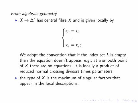
From algebraic geometry

I X→ ∆` has central fibre X and is given locally byxI1 = ti1

...

xI` = ti` ;

We adopt the convention that if the index set Ii is emptythen the equation doesn’t appear; e.g., at a smooth pointof X there are no equations. It is locally a product ofreduced normal crossing divisors times parameters;

I the type of X is the maximum of singular factors thatappear in the local descriptions;

10/69

I for k = [k1, . . . , k`], X [k] = x ∈ X : multxti = ki; for` = 1 we just write X [k] for the usual stratification of X ;

I smoothing of X as above is X→ S where X = Xs0 andthe fibres over S∗ are smooth and the monodromyrepresentation is abelian.

An example of a several parameter family is

X× X→ ∆×∆

which may be used to study natural classes, such as N , inHom

(H∗(Xη),H∗(Xη)

).

11/69

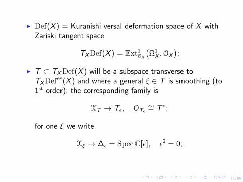
I Def(X ) = Kuranishi versal deformation space of X withZariski tangent space

TXDef(X ) = Ext1OX

(Ω1

X ,OX

);

I T ⊂ TXDef(X ) will be a subspace transverse toTXDef

es(X ) and where a general ξ ∈ T is smoothing (to1st order); the corresponding family is

XT → Tε, OTε∼= T ∗;

for one ξ we write

Xξ → ∆ε = SpecC[ε], ε2 = 0;

12/69

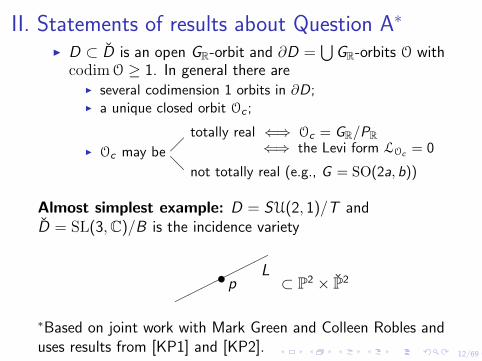
II. Statements of results about Question A∗

I D ⊂ D is an open GR-orbit and ∂D =⋃

GR-orbits O withcodimO ≥ 1. In general there are

I several codimension 1 orbits in ∂D;I a unique closed orbit Oc ;

I Oc may be

@

totally real ⇐⇒ Oc = GR/PR⇐⇒ the Levi form LOc = 0

not totally real (e.g., G = SO(2a, b))

Almost simplest example: D = SU(2, 1)/T andD = SL(3,C)/B is the incidence variety

t

pL⊂ P2 × P2

∗Based on joint work with Mark Green and Colleen Robles anduses results from [KP1] and [KP2].

13/69

Orbit structure is

D D ′′D ′

14/69

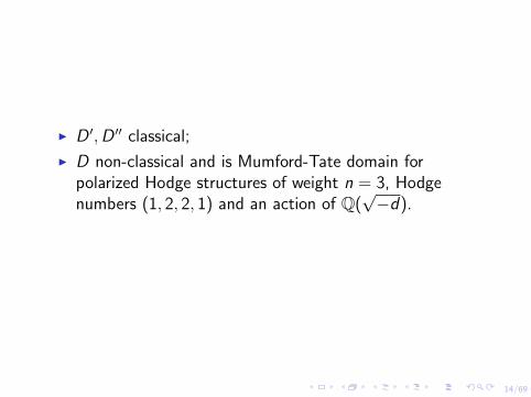
I D ′,D ′′ classical;

I D non-classical and is Mumford-Tate domain forpolarized Hodge structures of weight n = 3, Hodgenumbers (1, 2, 2, 1) and an action of Q(

√−d).

15/69

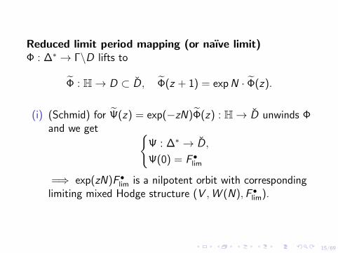
Reduced limit period mapping (or naıve limit)Φ : ∆∗ → Γ\D lifts to

Φ : H→ D ⊂ D, Φ(z + 1) = exp N · Φ(z).

(i) (Schmid) for Ψ(z) = exp(−zN)Φ(z) : H→ D unwinds Φand we get

Ψ : ∆∗ → D,

Ψ(0) = F •lim

=⇒ exp(zN)F •lim is a nilpotent orbit with correspondinglimiting mixed Hodge structure (V ,W (N),F •lim).

16/69

(ii) Set

F •∞ = limIm z→∞

Φ(z) = limIm z→∞

exp(zN) · F •lim ∈ ∂D

= limIm z→∞

exp(zN) · F •lim.

For B(N) = equivalence classes of (V ,W (N),F •)’s andB(N)R the R-split ones we have

B(N)

Φ∞

##HHH

HHHH

H

∂D

B(N)R

;;vv

vv

v

17/69

Then Φ∞ is holomorphic, factors as above, and ismaximal with respect to these properties.

N+

N

F •lim

F •∞

F •limHere, N ,Y ,N+ is an sl2.

18/69

r

r rr r rr rr?

?

?

?

Flim

rr rr r rr rr

@@@@@

@@@@@

F •∞ successivelypicks out the

highest powersof N

F∞

D classical =⇒ Φ∞ = GrW (extension data lost). In general,Φ∞ retains some but not all of the extension data

19/69

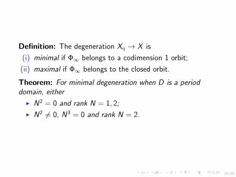
Definition: The degeneration Xη → X is

(i) minimal if Φ∞ belongs to a codimension 1 orbit;

(ii) maximal if Φ∞ belongs to the closed orbit.

Theorem: For minimal degeneration when D is a perioddomain, either

I N2 = 0 and rank N = 1, 2;

I N2 6= 0, N3 = 0 and rank N = 2.

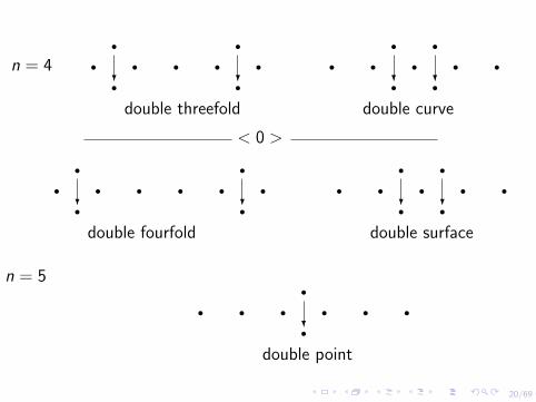
20/69

n = 4

rrr r?

r rrr r?

double threefold

r r r r r? ?

rr

rr

double curve

< 0 >

n = 5

rrr r?

r r rrr r?

double fourfold

r r r r r? ?

rr

rr

double surface

rrr r?

rr r rdouble point

21/69

For dim Xη = 5,x1x2 + x3x4 + x4x5 = 0 double point

x1x2 + x3x4 = 0 double surface

x1x2 = 0 double fourfold

Theorem′ [KP1] and [GGR]: For maximal deformations andgeneral Mumford-Tate domains

limiting mixed Hodge structure

is of Hodge-Tate type

⇐⇒ closed orbit is totally real.

22/69

It is elementary that a necessary, but in general not sufficient,condition is

hn,0 5 hn−1,1 5 · · · 5 hn−[n/2],[n/2].

Theorem′′: In the period domain case, if the closed orbit isnot totally real, then N = 2m is even and

I k 6= 0 =⇒ GrW (N)n+k,prim is Hodge-Tate;

I GrW (N)n+k,prim 6= 0 =⇒ k ≡ 2mod 4;

I GrW (N)n 6= 0 and the non-zero I p,qprim are Im+1,m−1

prim and

Im−1,m+1prim (no Im,mprim).

23/69

Example: n = 4 ss s?s s??s s??s s?s

(3, 1) (1, 3)

Picture a family of fourfolds Xη → X where Xη is a product ofpolarized K3 surfaces each of which has a type IIIdegeneration.

In general, for maximal degenerations, GrW (LMHS) is rigid.

24/69

Remarks:I The picture for general Mumford-Tate domains is more

complex, and in some ways more interesting. Forexample,

I G2 is singled out as an exception in the classification;I if there is a Hodge-Tate degeneration, then for

D = GC/P the Lie algebra p is an evenJacobson-Morosov parabolic.

25/69

I In general the Hodge-theoretic aspects of the GR-orbitstructure of ∂D may help guide the algebro-geometricproperties of boundary strata in a moduli problem

I curves and abelian varieties, K3 surfaces, cubicthreefolds and fourfolds (Laza) (these are all classicalD’s and only local normal crossings seem to occur),mirror quintics (non-classical D);

I more non-classical examples? e.g., quintic surfaces andthreefolds? May locally products of normal crossingvarieties occur as they do Hodge-theoretically?

26/69

I In the classical case Mumford et. al., and in the generalcase Kato-Usui have constructed maximal completions ofΓ/D’s

∆∗` // Γ/D

∩ ∩

∆` // Γ/DΣ, DΣ = toroidal object

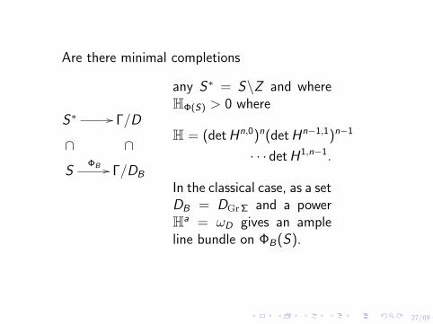
27/69

Are there minimal completions

S∗ // Γ/D

∩ ∩

SΦB // Γ/DB

any S∗ = S\Z and whereHΦ(S) > 0 where

H = (det Hn,0)n(det Hn−1,1)n−1

· · · det H1,n−1.

In the classical case, as a setDB = DGrΣ and a powerHa = ωD gives an ampleline bundle on ΦB(S).

28/69

III. Statements of results about

Questions B, B′, B′′∗

Definition: Ext1OX

(Ω1

X ,OX

)is the infinitesimal normal bundle

of X .

I For Ext1OX

(Ω1

X ,OX

)= E we have a stratification

X0 ⊃ X1 ⊃ · · · ⊃ X`, where if X 0k = Xk\Xk+1

E∣∣X 0k

is locally free of rank k .

∗Much of this was motivated by [Fr1].

29/69

Example: Locally X = X1 × X2 and stratification is

X1 × X2 ⊃ (X1,sing × X2) ∪ (X1 × X2,sing) ⊃ X1,sing × X2,sing.

Definition: E is trivializable if there are e1, . . . , e` ∈ H0(X ,E)such that for each connected component of X 0

k there areei1 , . . . , eik that frame E over that component;

I X = central fibre in X→ ∆` =⇒ Ext1OX

(Ω1

X ,OX

)is

trivializable with ei = dti .

30/69

Example: X = locally a normal crossing divisor. Then

I X = X0 ⊃ X1 = Xsing = DX ;

I Ext1OX

(Ω1

X ,OX

) ∼= ODX(X ) is the infinitesimal normal

bundle in [Fr1].

If DX =∐i=1

Di then ODX(X ) trivializable gives

ODX(X ) ∼=

⊕i=1

ODi

with sections 1Di∈ H0(ODi

).

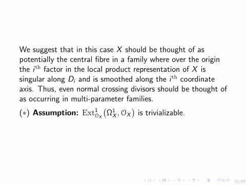
31/69

We suggest that in this case X should be thought of aspotentially the central fibre in a family where over the originthe i th factor in the local product representation of X issingular along Di and is smoothed along the i th coordinateaxis. Thus, even normal crossing divisors should be thought ofas occurring in multi-parameter families.

(∗) Assumption: Ext1OX

(Ω1

X ,OX

)is trivializable.

32/69

In the simpler case where X is locally a normal crossingdivisor, from the standard local to global spectral sequence forExt we have

C`

∼ =

TXDefes(X ) // TXDef(X )ρ // `⊕

iCDi

δ // H2(DerOX )

∼ = ∼ = ∼ = ∼ =

H1(Ext1

OX

(Ω1X ,OX

)) // Ext1OX

(Ω1X ,OX

) // H0(Ext1

OX

(Ω1X ,OX

)) // H2(ExtOX

(Ω1X ,OX

)).

33/69

Theorem I: Under the assumption (∗) there exists an`-parameter split limiting mixed Hodge structure with1Di↔ Ni .

This is defined in terms of X alone. In case δ = 0 andT ⊂ TXDef(X ) is unobstructed so that we have a family

X→ ∆`

where everything is smooth over X∗ → ∆∗`, the limiting mixedHodge structure is the associated graded to the one given bythe family.

We will explain below how the assumption ODi(X ) ∼= ODi

enters into the construction.

34/69

Still in the case where X = locally a normal crossing divisor,we have

Theorem II: Let TS ⊂ T be a k-dimensional subspace suchthat ρ(L) does not lie in any coordinate hyperplane in C`.Then there exists a k-parameter limiting mixed Hodgestructure whose commuting monodromies are linearcombinations of the 1Di

’s.

If there exists a family X→ S whose tangent space is TS ,then we obtain the limiting mixed Hodge structure associatedto this family.

In general we do not have S∗ = ∆∗`, as illustrated by thefollowing

35/69

Example: X0 = nodal variety of dimension 2n − 1 with nodesp1, . . . , p`;

X = X0 ∪(⋃

i=1

Xi

), Xi

∼= P2n−1 and X0 ∩ Xi = Qi

the normal crossing variety that would be the central fibre inthe standard semi-stable reduction of a smoothing of X0.Then the limiting mixed Hodge structure in Theorem I is theassociated graded to the one that would arise if we couldindependently smooth the nodes.

In Theorem II, the assumption just below it implies that X0

may be smoothed. Moreover, we have

TX0Def(X0) ∼= TXDef(X )

(to 1st order, deforming X0 is the same as deforming X )

36/69

and on L = ρ−1(coordinate hyperplanes in C`) subsets of thenodes may be smoothed

case ` = 3, k = 2

Monodromies are N1 + N2, N1 + N3, N2 + N3.

37/69

Three properties of nodal degenerations are

(i) the Koszul group H1(V ; N1, . . . ,N`) ∼= group ofrelations among the nodes;

(ii) the monodromy cone σ = σλ = ΣλiNi , λi > 0 isstrictly smaller than the polarizing cone

σpol =: σλ : W (Nλ) gives a polarized limiting mixedHodge structure

if, and only if, the nodes are dependent (relations amongnodes gives a larger polarizing cone);

(iii) there is an obstruction to extending the Ni to commutingsl2,i ’s in the split limiting mixed Hodge structure inTheorem I, and this obstruction vanishes if, and only if,the nodes are independent.

38/69

Example: Another example where DX has multiplecomponents is obtained by applying semi-stable reduction to apencil of surfaces Xt ⊂ P3 where the singularities of the baselocus are transverse intersections along the double curve of X0.These all contribute components to DX . Taking for examplethe familiar case when deg Xt = 4 all of the possible limitingmixed Hodge structures are extremal in the sense of thetheorem and may be pictured as

39/69

minimal, N2 = 0ss

sss17

? ?

X0 = Q1 ∩ Q2

maximal, N2 6= 0sss s18?

?

X0 = tetrahedron

which are familiar from the work of Kulikov, Friedman et al.(cf. [Fr1] and [Fr2]).

It may be that a similar story about extremal degenerationsholds in the work of Laza [La] on the cubic fourfold, but Ihaven’t had a chance to check this.

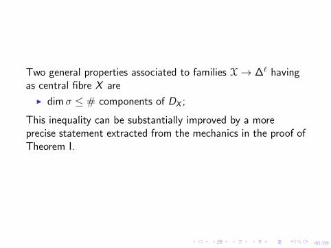
40/69

Two general properties associated to families X→ ∆` havingas central fibre X are

I dimσ ≤ # components of DX ;

This inequality can be substantially improved by a moreprecise statement extracted from the mechanics in the proof ofTheorem I.

41/69

For X locally a product of normal crossing divisors

I Na1i1· · ·Naj

ij= 0 if some ai > |Ii |, or if j > type of X .

This bounds from below the singularities that the central fibremust have in any semi-stable reduction of X∗ → ∆∗`. Thus, ifN1N2 6= 0 then X must somewhere be locally X1 × X2×(parameters) where X1 and X2 are singular.

Example: Hodge theory suggests that for some surfaces withpg = 2 the moduli space (if such exists) would have to includesingular surfaces of type k = 2.

42/69

One of our original motivations was to have a refined andcomputationally useful formulation for the period mapping atinfinity.

Example:

δ1 δ2 δ3

γ1 γ2 γ3 γ1 γ2 X

X• p1

• q1

• p2

• q2

Xt

43/69

For t = (t1, t2) and `(t) = (1/2πi)(log t1 + log t2) the periodmatrix is

Ω(t) =

1

1

1

`(t) + a11(t) a12(t) b1(t)

a21(t) `(t) + a22(t) b2(t)

b1(t) b2(t) c(t)

,

a12(t) = a21(t)

and Imc(t) > 0.

44/69

The nilpotent orbit is

11

1`(t) + a11 a12 b1

a21 `(t) + a22 b2

b1 b2 c

45/69

Rescaling gives a11 → a11 + λ1

a22 → a22 + λ2.

For the correspoinding equivalence class of limiting mixedHodge structures

ssss

s s??

Gr2

Gr1

Gr0

— (b1, b2) ∈ Ext1MHS(Gr0,Gr1)↔ AJ(pi − qi)

— c gives Gr1

— a12 = a21 gives part of the extension uponextension data for Gr2 over Gr0.

46/69

For ω1, ω2 = limt→0 ω1(t), ω2(t) where ω1(t), ω2(t) =normalized differentials of the 3rd kind

I aij =´ piqiωj , i 6= j ;

I may normalize ti , t2 to make the logarithmic singularitiescancel and have well defined a11, a22.

Refined dΩ has dc ; db1, db2; da12 and da11, da22.Moduli picture:

∂M3 ⊂M3 − dim = 6

∪C = codimension 2 boundary component

I dimC = 4 and c , b1, b2, a12 give local coordinates;

I a11, a22 give normal parameters to C ⊂M3.

47/69

Theorem: ξ ∈ Ext1OX

(Ω1

X ,OX

)defines a class

ξ(1) ∈ Ext1OX

(Ω1

Xξ/∆ε(log X )⊗ OX ,OX

),

and the refined differential of the period mapping at infinity isexpressed by the cup product

Ext1OX

(Ω1

Xξ/∆ε(log X )⊗ OX ,OX

)→ EndLMHSHn

(Ω•Xξ/∆ε(log X )⊗ OX

).

This is meant to give the flavor of the definition of andexpression for the refined differential of the period mapping atinfinity.

48/69

IV. Discussion of proofs

Question A ([GGR]): Builds on [KP1], [KP2] and the laterwork [GG]; main points include

I (V ,Q,F •)→ (g,B ,F •g ), g ⊂ EndQ(V );

I (V ,W ,F •)→ (V ,W , F •) with

I F •∞ = F •∞,

I (F •)g = (F •g );

49/69

I thus we may assumeVC = ⊕I p,q

gC = ⊕gp,q, I p,q = I q,p and gp,q = gq,p;

I then one matches the gp,q decomposition with thestandard root theoretic description of the orbit structure.

Questions B, B′, B′′: Recast and extend arguments in theliterature, including [Fr1], [Fr2], [St1], [PS],. . . in the1-parameter case. Some work in the `-parameter case hasbeen done in [Fu].

50/69

Example: In the 1-parameter case, E p,q1 terms are sums of

groups Ha(X [b])(−c) where

I d1 is expressed in terms of various restriction and Gysinmaps;

I E2 = E∞ = Gr(LMHS).

Convenient to picture a split limiting mixed Hodge structure interms of N-strings

H0(−m)→ · · · · · · · · · · · · → H0(−1)→ H0

H1(−1)→ · · · → H1

...

Hm

where Nk = Hodge structure of weight k .

51/69

Theorem: If OD(X ) ∼= OD , there are complexes

Hq−4(X [k+2])(−2)

⊕ Hq−2(X [k+1])(−1)

→ Hq−2(X [k])(−1) → ⊕ → Hq(X [k])

⊕ Hq(X [k−1])

Hq(X [k−2])

such that for 0 5 j 5 m − i the terms in the N-strings are

Hm−i(−j) ∼= (H∗Rest“+” H∗Gy)(Hm−i(X [i+1])

)(−j).

Moreover, the monodromy N = N1 + · · ·+ N` is induced by

N =∑i

1Di(1)

52/69

where for b = 2, X [b] =∐

i X[b]i and

Ha(X

[b]i

)(−c)

1Di∼−→ Ha

(X

[b]i

)(−(c − 1)).

The important observation is that having trivializations

ODi(X ) ∼= ODi

implies thatGy ·Rest = −Rest ·Gy,

so that the diagram in the statement of the theorem isactually a complex.

53/69

A perhaps new ingredient is the observation that the Ndecomposes as Σ1Di

(1). As in Theorem II we may then definean `-parameter 1st order family and Nλ = ΣλiNi , λi 6= 0. Herethe 1Di

correspond to a trivialization ODi(X ) ∼= ODi

and meansthat to 1st order we have a specified parameter in thesmoothing of the component Di of XSing. We also have ansl2,i acting on E1 where

Yi = (2c − b + 1)1Di

on Ha(X[b]i )(−c), b = 2. Then for Y = ΣYi ,

[d1,Y ] = −d1

so that Y acts on E2 = E∞ = GrW (N) V .

54/69

In general [d1,Yi ] + d1 6= 0 and measures the linking betweenvanishing cycles and their duals associated to differentcomponents of Xsing. This gives a geometric description of theobstructions to having commuting sl2,i ’s acting on GrW (N) V .

Example:

none commuting sl2’s

commuting sl2’s

In both cases GrW (LMHS) is the same over Q.

55/69

For general X = locally a product of normal crossing varietiesthere are a few additional points that arise.

A first step is a fairly straightforward extension from the case` = 1 of the identification for families X→ ∆`,

Hn(Xη) ∼= Hn(Ω•X/∆`(log X )⊗ OX

).

The complex Ω•X/∆`(log X )⊗ OX depends only on

T0∆` ⊂ TDef(X ) and is identified as the cokernel of the

map

Ω•X(log X )dt1/t1∧···∧dt`/t`−−−−−−−−−→ Ω•+`X (log X ),

which can be defined in terms of T0∆` alone. Note the

`-fold wedge product here.

56/69

A second point is that the Ni are defined in terms of theconnected components in the highest dimensional strata of thesupport of Ext1

OX(Ω1

X ,OX ).

One subtlety is that as in the case ` = 1 one cannot define aweight filtration on the complex Ω•X(log X )⊗ OX . To have amonodromy weight filtration W , whose Wk are expressed onE1 by linear inequalities among a, b, c , on Hn

lim the indices haveto have length 2n + 1, and we can only get n + 1 out of theusual filtration on Ω•X(log X ). The correct thing to do issuggested by the map above, which is the first term in aresolution of Ω•X(log)⊗ OX from which some numerologysuggests what the weight filtration should be.

57/69

A central point is to use the hard Lefschetz theorem on thenormalized strata of X and both Hodge-Riemann bilinearrelations to deduce that W , which easily satisfies

Nλ : Wk → Wk−2,

for all λ in fact satisfies

Nkλ : Wk

∼−→ W−k

when k = 0 and λ = (λ1, . . . λ`), λi > 0. Without this fromthe weight filtration W we get a mixed Hodge structure butnot a limiting mixed Hodge structure with W = W (N). Theproof of the result involves extending the nice argument due toGuillen and Navaro Anzar to the several parameter case.

58/69

V. Final remarks

In closing there were three classical properties of monodromycones for degenerating families of Hodge structures, predictedby Deligne (and established by him in the `-adic setting andproved in the Hodge-theoretic setting in [CKS1], [CKS2]).

(a) W (Nλ) is independent of λ with λi > 0;

(b) W (N) is a relative weight filtration for W (Ni);

(c) the Koszul groups Hi(V ; N1, . . . ,N`) vanish in positiveweight (purity).

59/69

The statement (b) means that we easily have thatN : Wk(Ni)→ Wk−2(Ni), and then the much more subtleresult, whose proof uses Hodge-Riemann I, II,

W (N) induces W(

N∣∣GrW (Ni )

)on GrW (Ni )

is true. It follows from this and the above construction that,e.g., when ` = 2 we have the picture

60/69

6

variation of mixed Hodge structureinduced by X∗1 → ∆∗1 × 0

?

induced variation of mixedHodge structure in the sense of [S]

variation of Hodge structureassociated to X∗ → ∆∗1 ×∆∗2

and the limiting mixed Hodge structure “limt→0(t, t)” alongthe dotted line may be identified with “limt1→0 limt2→0.” Thisresult is true by Deligne’s argument in the `-adic case; thegeometric argument may be useful in the computation ofexamples.

61/69

The result (b) means that the C[Ns , . . . ,Nλ]-module V hasvery special properties. For example, it implies that as aC[Nλ,Ni ]-module it is a direct sum of C[Nλ,Ni ]/(Np

λ ,Nqi )’s.

These statements can be verified using the above, which givessome slight refinements. For instance in the example of anodal X0

(iv) the weight filtration W (Nλ) is independent of theλi ∈ C∗ if, and only if, the nodes are independent.

62/69

Another motivation for the above is this: Given a nilpotentN ∈ End(V ), Robles has formulated and proved a preciseresult which has as a corollary that N is the monodromy of avariation of Hodge structure over ∆∗ constructed in an explicitway from (N ,V ). One may ask

Given commuting Ni ∈ End(V ), isσ = spanR>0N1, . . . ,N` that satisfies (a), (b), (c)above a monodromy cone?

63/69

She has shown by example that when ` > 1 this may not bethe case. This of course raises the question: can one findadditional conditions that σ be a monodromy cone? By havingan explicit description of σ in the geometric case one mighthope to identify additional conditions, but so far this has notbeen carried out.

64/69

We conclude with a final speculative comment. On GrW Vthere is an induced action of the Nλ and N1, . . . ,N`. For eachλ with the λi > 0 we have Nλ,Y ,N

+λ giving an

sl2,λ ⊂ End(GrW V ), and by a result of Looijenga-Lunts(whose proof uses Hodge-Riemann I, II) these sl2,λ’s generatea semi-simple Lie algebra gσ ⊂ End(GrW V ).

We have noted above that in the geometric case the Yi for Ni

do not in general pass to E2 = GrW V . However, a linearalgebra construction of Deligne gives canonically a set Y ′i ofgrading elements for the Ni , and from this we obtain a set ofsl2,i ’s. These generate a Lie algebra g′σ ⊂ End(GrW V ), onethat in the geometric case measures the obstruction to havingthe commuting sl2,i ’s on E1 survive to GrW V .

65/69

In some examples, using the polarization conditions, one mayshow that

gσ = g′σ.

If true in general the condition

(d) g′σ is semi-simple

should then be added to the properties of monodromy cones.

—Thank you—

66/69

ReferencesThe main references for Question A are

[KP1] M. Kerr and G. Pearlstein, Boundary components ofMumford-Tate domains. arXiv:1210.5301.

[KP2] M. Kerr and G. Pearlstein, Naıve boundary strata andnilpotent orbits, preprint, 2013.

[GGR] M. Green, P. Griffiths, and C. Robles, Extremaldegenerations of polarized Hodge structures,arxiv:1403.0646.

67/69

[GG] M. Green and P. Griffiths, Reduced limit period mappingsand orbits in Mumford-Tate varieties, to appear in theHerb Clemens volume.

So far as Question B is concerned, it mainly consists of proofanalysis and extension of the works

[Fr1] R. Friedman, Global smoothings of varieties with normalcrossings, Ann. of Math. 118 (1983), 75–114.

[Fr2] R. Friedman, The period map at the boundary of moduli,in Topics in Transcendental Algebraic Geometry,183–208, (P. Griffiths, ed.), Princeton Univ. Press,Princeton, NJ, 1984.

[La] R. Laza, The moduli space of cubic fourfold via theperiod map, Ann. of Math 172 (2010), 673–711.

68/69

[Fu] T. Fujisawa, Mixed Hodge structures on log smoothdegenerations, Tohoku Math. 60 (2008), 71–100.

[St1] J. Steenbrink, Limits of Hodge structures, Invent. Math.31 (1979), 229–257.

[SZ] J. Steenbrink and S. Zucker, Variation of mixed Hodgestructure. I, Invent. Math. 80 (1985), 489–542.

69/69

The Hodge-theoretic aspects of the discussion are based on

[CK] E. Cattani and A. Kaplan, Polarized mixed Hodgestructures and the local monodromy of a variation ofHodge structure, Invent. Math. 67 (1982),

CKS1] E. Cattani, A. Kaplan, and W. Schmid, Degenerations ofHodge structures, Ann. of Math. 123 (1986), 457–535.

[CKS2] E. Cattani, A. Kaplan, and W. Schmid, L2 andintersection cohomologies for a polarizable variation ofHodge structure, Invent. Math. 87 (1987), 217–252.

There are of course many related works that are not listedabove.