Universite Catholique de LouvainFaculty of applied sciences

Department of computer sciencesMaster thesis 2007

Algebraic soft-decoding

of

Reed-Solomon codes

Arnaud Dagnelies

Promoter:Prof. P. Delsarte

Thanks to my parents,my promoter,

all my roommatesand especiallyAmine, Ciara,

Camille, Netah,Yo-Sun and Yo-Yin

1

Foreword

This text is divided in two parts. The first one, the prerequisites, introducesall the necessary concepts of coding theory. If the reader is familiar withthe basics of information and coding theory, he might skip this part and godirectly to the second part, which is the core of this thesis. This second partstudies an algorithm which improves the decoding of Reed-Solomon codes.For readers familiar with coding theory, the second part is gently introducedalso making it directly accessible.

Error-correcting codes are used to add redundancy to data to make itfault tolerant (up to a certain degree). Roughly said, the typical way to do itis to encode sequences of bits to longer sequences of bits by adding structuredredundancy in it. That way, even if some bits are corrupted, but not toomany, the structured redundancy enables us to retrieve the original data.One of the most efficient and widely used type of error-correcting codes areprecisely Reed-Solomon codes. Both because of their good properties andtheir efficient decoding techniques. The algorithm presented here runs inpolynomial time and provides more powerful decoding than conventionaldecoding algorithms. A more precise and exhaustive description can befound in the introduction of the second part of this text.

We wish you an enjoyable reading.

2

Contents

I Prerequisites 6

1 Introduction 71.1 Overview . . . . . . . . . . . . . . . . . . . . . . . . . . . . . 71.2 Introductory example . . . . . . . . . . . . . . . . . . . . . . 8

2 Basics of communication 92.1 Communication system . . . . . . . . . . . . . . . . . . . . . 92.2 In more details... . . . . . . . . . . . . . . . . . . . . . . . . . 112.3 Channel encoder . . . . . . . . . . . . . . . . . . . . . . . . . 132.4 Channels and demodulators . . . . . . . . . . . . . . . . . . . 14

2.4.1 Binary Gaussian channel ...and friends . . . . . . . . . 142.4.2 Qary symmetric channel . . . . . . . . . . . . . . . . . 162.4.3 Binary erasure channel . . . . . . . . . . . . . . . . . . 17

2.5 Channel decoder . . . . . . . . . . . . . . . . . . . . . . . . . 17

3 Coding theory introduction 193.1 What are codes? . . . . . . . . . . . . . . . . . . . . . . . . . 193.2 Nearest neighbor decoding . . . . . . . . . . . . . . . . . . . . 203.3 Space and spheres . . . . . . . . . . . . . . . . . . . . . . . . 22

4 Mathematics fundamentals 274.1 Groups . . . . . . . . . . . . . . . . . . . . . . . . . . . . . . . 274.2 Rings . . . . . . . . . . . . . . . . . . . . . . . . . . . . . . . 304.3 Fields . . . . . . . . . . . . . . . . . . . . . . . . . . . . . . . 32

5 Linear codes 345.1 Definition . . . . . . . . . . . . . . . . . . . . . . . . . . . . . 345.2 Hard decoding using the syndrome . . . . . . . . . . . . . . . 38

3

6 More on fields 426.1 Field properties . . . . . . . . . . . . . . . . . . . . . . . . . . 426.2 The extended Euclidean algorithm . . . . . . . . . . . . . . . 44

7 Reed-Solomon codes 487.1 Not so classical decoding . . . . . . . . . . . . . . . . . . . . . 507.2 The key equation . . . . . . . . . . . . . . . . . . . . . . . . . 547.3 Conclusion . . . . . . . . . . . . . . . . . . . . . . . . . . . . 57

II Soft decoding 58

8 Introduction 598.1 What do we achieve here? . . . . . . . . . . . . . . . . . . . . 598.2 History and results . . . . . . . . . . . . . . . . . . . . . . . . 598.3 General outline . . . . . . . . . . . . . . . . . . . . . . . . . . 60

9 The Sudan algorithm 619.1 Introduction . . . . . . . . . . . . . . . . . . . . . . . . . . . . 619.2 Decoding problem reformulation . . . . . . . . . . . . . . . . 619.3 Weighted degree . . . . . . . . . . . . . . . . . . . . . . . . . 649.4 Overview . . . . . . . . . . . . . . . . . . . . . . . . . . . . . 649.5 Constraints for Q . . . . . . . . . . . . . . . . . . . . . . . . . 659.6 Monomial enumeration . . . . . . . . . . . . . . . . . . . . . . 669.7 Roots vs degree of Q . . . . . . . . . . . . . . . . . . . . . . . 679.8 Example . . . . . . . . . . . . . . . . . . . . . . . . . . . . . . 689.9 Performances . . . . . . . . . . . . . . . . . . . . . . . . . . . 69

10 Zeros, roots and constraints 7110.1 Zeros of higher multiplicity . . . . . . . . . . . . . . . . . . . 7110.2 Expressing the constraints . . . . . . . . . . . . . . . . . . . . 73

11 The core theorem 7711.1 Multiplicity Matrix . . . . . . . . . . . . . . . . . . . . . . . . 7711.2 Algorithm and example . . . . . . . . . . . . . . . . . . . . . 80

12 Multiplicity assignment 8412.1 The reliability matrix . . . . . . . . . . . . . . . . . . . . . . 8412.2 Setting the problem . . . . . . . . . . . . . . . . . . . . . . . 8512.3 Greedy MAA . . . . . . . . . . . . . . . . . . . . . . . . . . . 8712.4 Proportional MAA . . . . . . . . . . . . . . . . . . . . . . . . 88

4

12.5 Asymptotic hard-decoding performances . . . . . . . . . . . . 8912.6 Asymptotic soft-decoding performances . . . . . . . . . . . . 90

13 Kotter’s interpolation 9213.1 Monomial ordering . . . . . . . . . . . . . . . . . . . . . . . . 9213.2 Kernels of constraints . . . . . . . . . . . . . . . . . . . . . . 9413.3 The algorithm . . . . . . . . . . . . . . . . . . . . . . . . . . . 9413.4 Performances . . . . . . . . . . . . . . . . . . . . . . . . . . . 9913.5 Pseudo-code . . . . . . . . . . . . . . . . . . . . . . . . . . . . 99

14 Factorization 10114.1 Roth-Ruckenstein factorization . . . . . . . . . . . . . . . . . 10114.2 Pseudo-code . . . . . . . . . . . . . . . . . . . . . . . . . . . . 104

15 Program notes 10615.1 Algebra . . . . . . . . . . . . . . . . . . . . . . . . . . . . . . 107

15.1.1 Finite fields . . . . . . . . . . . . . . . . . . . . . . . . 10715.2 Polynomials . . . . . . . . . . . . . . . . . . . . . . . . . . . . 10815.3 Communication System . . . . . . . . . . . . . . . . . . . . . 108

15.3.1 Interfaces . . . . . . . . . . . . . . . . . . . . . . . . . 10815.3.2 Channels . . . . . . . . . . . . . . . . . . . . . . . . . 10915.3.3 Encoders and decoders . . . . . . . . . . . . . . . . . . 110

16 Conclusion 111

III Appendix 116

A Source code 117A.1 Algebra . . . . . . . . . . . . . . . . . . . . . . . . . . . . . . 117A.2 Communication system interfaces . . . . . . . . . . . . . . . . 131A.3 Reed-Solomon encoders/decoders . . . . . . . . . . . . . . . . 133A.4 Channels . . . . . . . . . . . . . . . . . . . . . . . . . . . . . 148

5

Part I

Prerequisites

6

Chapter 1

Introduction

1.1 Overview

Reliable communication has always been important. Even in our every daylife. Imagine your mail has a few kilobytes of data altered on its way, orthat an extremely tiny scratch makes your DVD unreadable, or that themessage typed on your mobile phone was sent with wrong letters or to awrong recipient... All these are examples of error detection or correction.In our era of digital communication, reliable transmission of informationis a wide ranging concern. It is the aim of this first part to establish amodel of communication, to explain precisely how it can be modeled andhow exactly the information can be made more reliable by means of error-correcting codes. To go straight to the subject, a little introductory exampleis presented thereafter. Then, a communication system model is taken in allits generality in the second chapter. The role of the different componentsare inspected and refined at each step, by using basic assumptions on thekind of communication models. Most notably, bloc encoders, memorylesschannels are reviewed with an emphasis on the distinction between hard andsoft-information. Then the basics of coding theory is presented in chapter 3,also in all its generality, along with some bounds on code sizes and decodingparadigms. Before linear codes are reviewed (these are the codes having thegreatest use in practice), fundamental mathematics are reviewed in chapter4. This includes a basic coverage of groups, rings and fields. This enables usto present linear codes in chapter 5 as vector subspaces over finite fields pre-viously presented. This chapter also covers the generator and parity checkmatrices as well as a brief introduction to syndrome decoding. Then, inchapter 6, finite fields at looked more closely at, explaining basic properties,

7

reviewing polynomials with coefficient in finite fields, how to construct ex-tension fields and lastly the extended Euclidean algorithm which will showits use in the next chapter. It the last chapter 7, Reed-Solomon codes, thesubject of the second part, are introduced. It explains what Reed-Solomoncodes are, how to decode them using classical algorithms and presents thekey equation.

1.2 Introductory example

So, what is it all about?

Let us begin with a simple illustrative example. Imagine a satellite in spacewhich communicates with some station on earth. That is, it receives dataor sends data messages across space. Let us take a basic scenario wherethe station on earth sends a binary message to it, for example 00110. Thismessage is then transformed by a modulator to produce waves that thesatellite receives and demodulates to recover the original message. Thecatch is that interferences in space can provoke misinterpretations by thedemodulation which in turns causes erroneous bits in the received message.Still with the example that 00110 was sent, the erroneous message 10110could be received instead. In the best case scenario, the satellite wouldask for a retransmission and in the worst case, it would execute a wrongcommand with possible potentially disastrous consequences.

Since a retransmission is fairly time consuming, one could wonder ifthere is no better way to transmit information more reliably. And this isexactly what coding theory is about. By adding redundancy in messages, itis possible to detect or even recover the original message if the distortion isnot too important. For example, every bit of the message could be repeatedthree times so that the message 00110 would be encoded in 000 000 111 111000. That way, if 010 000 111 111 000 is received the correct message couldbe easily decoded by selecting the bit with greatest occurrence from eachtriplet. The whole question of coding theory is about how to add redun-dancy in messages to achieve the best compromises between the quantityof redundancy added and the error-correction ability it provides. Knowingthe channel, the demodulator can often provide the information about theprobabilities of whether each bit is 0 or 1. This opens the way to more pow-erful soft decoding techniques taking advantage of this information. One ofthis techniques is the subject of this thesis.

8

Chapter 2

Basics of communication

”The fundamental problem of communication is that of repro-ducing at one point either exactly or approximately a messageselected at another point.”

Claude E. Shannon - A Mathematical Theory ofCommunication

2.1 Communication system

Communication is the activity of transmitting information. This transmis-sion can either be made between two places, like a phone call. Or betweentwo points in time, for example the writing of this thesis so that it can beread later on. We shall restrict ourselves to the study of digital communi-cation. That is, the transmission of messages that are sequences of symbolstaken from a set called alphabet.

Definition 1 An alphabet A is a (finite or infinite) set of symbols. Bywriting Aq, we denote a finite alphabet having exactly q distinct symbols.

ExampleA message on an alphabet 0, 1 could be ”01001110” as in the introductoryexample. Or the sentence ”HELLO WORLD” with the alphabet of usualEnglish alphabet augmented by the space character.

9

Digital communication has become predominant in today’s world. Itranges from internet, storage disks, satellite communication to digital tele-vision and numerous others... Moreover, any analog system can be trans-formed into digital data by various sampling and signal transformation meth-ods. Typical examples include encoding music in an mp3, numerical cam-eras, voice recognition and many others.

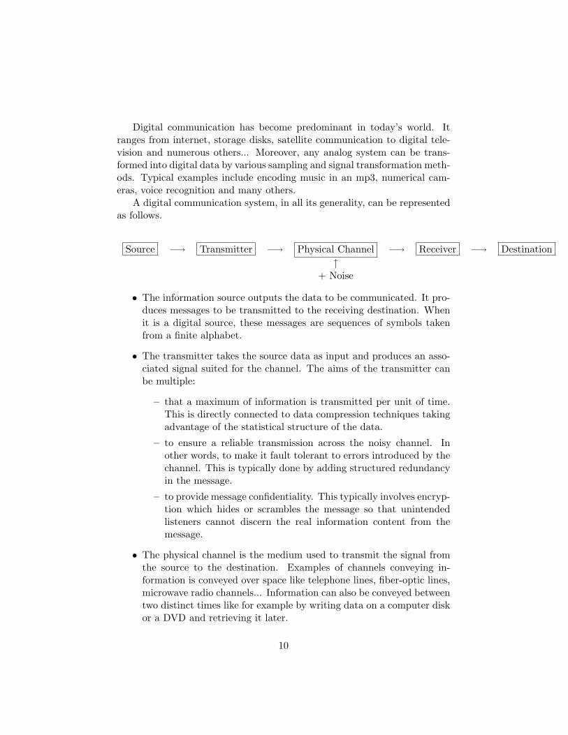
A digital communication system, in all its generality, can be representedas follows.

Source −→ Transmitter −→ Physical Channel −→ Receiver −→ Destination↑

+ Noise

• The information source outputs the data to be communicated. It pro-duces messages to be transmitted to the receiving destination. Whenit is a digital source, these messages are sequences of symbols takenfrom a finite alphabet.

• The transmitter takes the source data as input and produces an asso-ciated signal suited for the channel. The aims of the transmitter canbe multiple:

– that a maximum of information is transmitted per unit of time.This is directly connected to data compression techniques takingadvantage of the statistical structure of the data.

– to ensure a reliable transmission across the noisy channel. Inother words, to make it fault tolerant to errors introduced by thechannel. This is typically done by adding structured redundancyin the message.

– to provide message confidentiality. This typically involves encryp-tion which hides or scrambles the message so that unintendedlisteners cannot discern the real information content from themessage.

• The physical channel is the medium used to transmit the signal fromthe source to the destination. Examples of channels conveying in-formation is conveyed over space like telephone lines, fiber-optic lines,microwave radio channels... Information can also be conveyed betweentwo distinct times like for example by writing data on a computer diskor a DVD and retrieving it later.

10

As the signal propagates through the channel, or on its storage place,it may be corrupted. For example, the telephone lines suffer fromparasitic currents, waves are subject to interference issues, a DVD canbe scratched... But these perturbations are regrouped under the termof noise. The more noise, the more the signal is altered and the more itis difficult to retrieve the information originally sent. Of course, thereare many other reasons for errors like timing jitter, attenuation dueto propagation, carrier offset... But all these perturbations lie beyondthe scope of this thesis.

• The receiver ordinarily performs the inverse operation done by thetransmitter. It reconstructs the original message from the receivedsignal.

• The destination is the system or person for whom the message is in-tended.

2.2 In more details...

As was said in the previous section, the transmitter can have several rolestogether. To compress data, to secure data, to make it more reliable andlastly to transmit it as signals suited for the physical channel. Compressingdata is also called source coding, it consists of mapping sequences of symbolsin the original data stream to shorter ones. This is done based on thestatistical distribution of the original data: the most frequent sequences aremapped to shorter ones while rare sequences are mapped to longer ones. Bydoing this, the resulting sequences are on average shorter, i.e. sequences withless symbols. On the opposite, in order to make the sequence of symbolsrobust to errors, redundancy is added to it. This is called channel encodingand consists of mapping shorter sequences to longer ones so that if a fewsymbols are corrupted the original data can nevertheless be found back.

What if we want the transmitter to do both? This seems contradictorysince one reduces the number of sent symbols while the other increasesit. However, it is not really. The source coding reduces the redundancyof unstructured data which would not provide protection if symbols werecorrupted. For example, despite knowing that a file contains on average99% of zeros, you cannot know which bits were corrupted when sending thefile as it is.

On the opposite, channel coding adds structured data to improve protec-tion against such errors during the transmission. By taking the compressed

11

file and reapeating three times each bit, you can decode correctly up to oneerror per three bits introduced.

One could wonder if a technique performing both in a single step couldbe more efficient than doing it it sequentially. It turns out that performingsource and channel coding sequentially tends to be optimal when the treatedsequence length tends to infinity. This is known as the source-channel codingseparation theorem and is one of the results of Shannon’s ground breakingwork [4]. For finite sequence length, such joint encoding techniques are stilla subject of research.

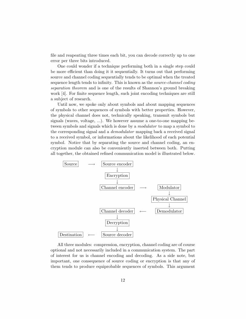
Until now, we spoke only about symbols and about mapping sequencesof symbols to other sequences of symbols with better properties. However,the physical channel does not, technically speaking, transmit symbols butsignals (waves, voltage, ...). We however assume a one-to-one mapping be-tween symbols and signals which is done by a modulator to map a symbol tothe corresponding signal and a demodulator mapping back a received signalto a received symbol, or informations about the likelihood of each potentialsymbol. Notice that by separating the source and channel coding, an en-cryption module can also be conveniently inserted between both. Puttingall together, the obtained refined communication model is illustrated below.

Source −→ Source encoder↓

Encryption↓

Channel encoder −→ Modulator↓

Physical Channel↓

Channel decoder ←− Demodulator↓

Decryption↓

Destination ←− Source decoder

All three modules: compression, encryption, channel coding are of courseoptional and not necessarily included in a communication system. The partof interest for us is channel encoding and decoding. As a side note, butimportant, one consequence of source coding or encryption is that any ofthem tends to produce equiprobable sequences of symbols. This argument

12

will support an important assumption for the input of the channel encoderlater on. Moreover, even if these modules are not present and nothing isknown about the source’s output, this is still the best assumption that canbe made. The main part of interest for us is the channel encoder and decoderand it can now be isolated from the remaining system.

Lastly, the modulator and demodulator constitute the glue between thetransmitter, the physical channel and the receiver. Usually, the channelis considered as the modulator, the physical channel and the demodulatortogether, providing an abstract model having as input and output symbols.However, the received signals, altered by noise, may not match any of thesent ones. So either it is mapped to other symbols in a bigger alphabet orsome threshold decision must be used to decide which symbol of the originalalphabet it should be. This is seen in more details in the section aboutchannels.

2.3 Channel encoder

The role of the encoder is to add structured redundancy to sequences ofsymbols. There are different ways of doing this but the biggest class ofencoders are by far block encoders. They work by cutting the data stream inblocks (of symbols) of fixed size and encoding these blocks one after another.Such a block, a finite sequence of symbols, is also known as a word.

Definition 2 A word w = (w1, ..., wm) of length m over an alphabet A isan ordered sequence of m symbols taken from A.

The data block is called the message word. By hypothesis, it has a fixedlength, say k. The encoder maps each such word to a longer one, calledcodeword, also of fixed size, say n. A reasonable assumption is that bothwords, the message and the encoded codeword, are defined over the samealphabet Aq. The encoder is thus a mapping from words of length k towords of length n where n > k. Words can be seen as points in a spaceover the alphabet. In this light, the encoder is a mapping of points in Akqto points in Anq . More specifically, the encoder is an injective function:

Enc : Akq → C ⊂ Anq .

If the alphabet has q elements, then qk message words are mapped ontoqk from qn possible words. The set of all codewords is thus only a subset ofAnq and this set forms the code C ⊂ Anq which is the image of the encoder

13

function. On a closer look, it turns out that what is of interest is not themapping, but the code C itself. This is the subject of the next chapter.

2.4 Channels and demodulators

Channels are the medium used to transmit signals corresponding to symbols,where the transmission of each symbol is assumed to be of equal duration.When noise corrupts a transmitted symbols, it tends to introduce errorshaving some pattern. One of the most frequent pattern is burst errors:several consecutive symbols are usually corrupted at once. Other patternsinclude cyclic errors, ”echoing” errors and so on. However, we shall restrictourselves only to channel models introducing errors randomly, without anypattern. These are called memoryless channels.

Definition 3 In a memoryless channel, the nth received symbol yn dependssolely on the nth sent symbol xn.

Thus, in such a channel, each symbol is transmitted, and maybe cor-rupted, independently from the others. The model of any memoryless chan-nel can be characterized by:

• An input alphabet Ain: the set of symbols that can be sent on thechannel.

• An output alphabet Aout: the set of symbols that can be received atthe other end of the channel.

• Transition probabilities p(Y = y|X = x) for all x ∈ Ain, y ∈ Aout,denoting the probability of receiving the symbol y when x was sent.

The reason transition probabilities can be expressed this way lies inthe fact that the channel is memoryless. For channels with memory, morecomplex stochastic models would be needed and the transition probabilitieswould rely on several variables.

Concerning the input and output alphabets, they are not necessarily thesame. The output alphabet can even be infinite despite Ain is finite. Thisis illustrated in the channel presented just now.

2.4.1 Binary Gaussian channel ...and friends

The Binary Gaussian channel is one of the most used in practice. In thissection we present a slight variation thereof. Let its input alphabet be 0, 1

14

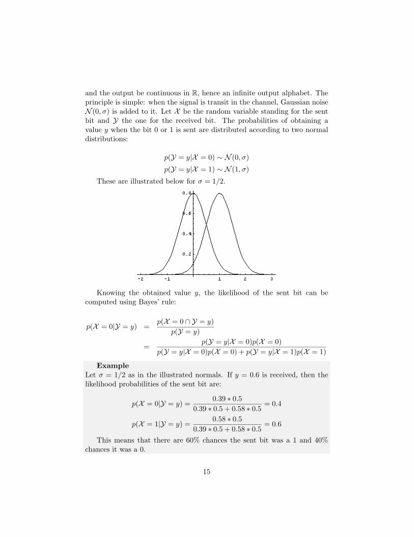
and the output be continuous in R, hence an infinite output alphabet. Theprinciple is simple: when the signal is transit in the channel, Gaussian noiseN (0, σ) is added to it. Let X be the random variable standing for the sentbit and Y the one for the received bit. The probabilities of obtaining avalue y when the bit 0 or 1 is sent are distributed according to two normaldistributions:

p(Y = y|X = 0) ∼ N (0, σ)

p(Y = y|X = 1) ∼ N (1, σ)

These are illustrated below for σ = 1/2.

Knowing the obtained value y, the likelihood of the sent bit can becomputed using Bayes’ rule:

p(X = 0|Y = y) =p(X = 0 ∩ Y = y)

p(Y = y)

=p(Y = y|X = 0)p(X = 0)

p(Y = y|X = 0)p(X = 0) + p(Y = y|X = 1)p(X = 1)

ExampleLet σ = 1/2 as in the illustrated normals. If y = 0.6 is received, then thelikelihood probabilities of the sent bit are:

p(X = 0|Y = y) =0.39 ∗ 0.5

0.39 ∗ 0.5 + 0.58 ∗ 0.5= 0.4

p(X = 1|Y = y) =0.58 ∗ 0.5

0.39 ∗ 0.5 + 0.58 ∗ 0.5= 0.6

This means that there are 60% chances the sent bit was a 1 and 40%chances it was a 0.

15

The knowledge of the likelihood of the sent bit is called soft-information,in the example 40% and 60%. This is in opposition to hard-informationwhich is the knowledge of only the most likely symbol. For the previousexample, just 1. The latter alternative is simpler for the demodulator sincea simple threshold rule tells if the output should be a zero or a one. If theinput of the channel is assumed to be equiprobable, then the output is 0 ify < 0.5 else it is 1. However, by doing this, some information is inherentlylost. On the opposite, no information is lost in soft-information consistingof the likelihood of each symbol.

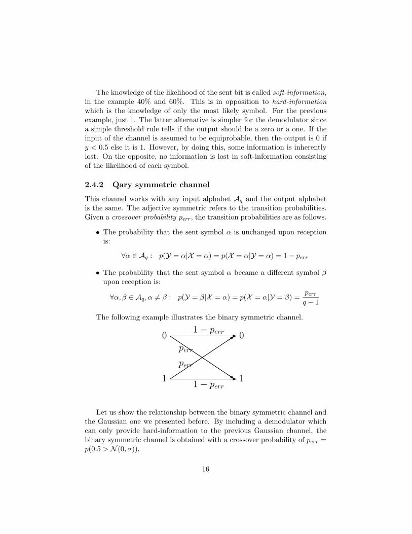
2.4.2 Qary symmetric channel

This channel works with any input alphabet Aq and the output alphabetis the same. The adjective symmetric refers to the transition probabilities.Given a crossover probability perr, the transition probabilities are as follows.

• The probability that the sent symbol α is unchanged upon receptionis:

∀α ∈ Aq : p(Y = α|X = α) = p(X = α|Y = α) = 1− perr

• The probability that the sent symbol α became a different symbol βupon reception is:

∀α, β ∈ Aq, α 6= β : p(Y = β|X = α) = p(X = α|Y = β) =perrq − 1

The following example illustrates the binary symmetric channel.

-

-

QQQQQQQQQQs

3

0 0

1 1

perr

1− perr

1− perr

perr

Let us show the relationship between the binary symmetric channel andthe Gaussian one we presented before. By including a demodulator whichcan only provide hard-information to the previous Gaussian channel, thebinary symmetric channel is obtained with a crossover probability of perr =p(0.5 > N (0, σ)).

16

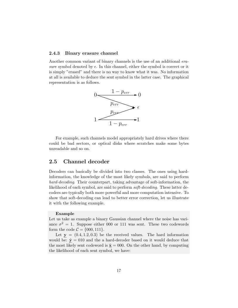
2.4.3 Binary erasure channel

Another common variant of binary channels is the use of an additional era-sure symbol denoted by ε. In this channel, either the symbol is correct or itis simply ”erased” and there is no way to know what it was. No informationat all is available to deduce the sent symbol in the latter case. The graphicalrepresentation is as follows.

-

-

1

PPPPPPPPPPq

0 0

1 1

perr

perr

1− perr

1− perr

ε

For example, such channels model appropriately hard drives where therecould be bad sectors, or optical disks where scratches make some bytesunreadable and so on.

2.5 Channel decoder

Decoders can basically be divided into two classes. The ones using hard-information, the knowledge of the most likely symbols, are said to performhard-decoding. Their counterpart, taking advantage of soft-information, thelikelihood of each symbol, are said to perform soft-decoding. These latter de-coders are typically both more powerful and more computation intensive. Toshow that soft-decoding can lead to better error correction, let us illustrateit with the following example.

ExampleLet us take as example a binary Gaussian channel where the noise has vari-ance σ2 = 1. Suppose either 000 or 111 was sent. These two codewordsform the code C = 000, 111.

Let y = (0.4, 1.2, 0.3) be the received values. The hard informationwould be: y = 010 and the a hard-decoder based on it would deduce thatthe most likely sent codeword is x = 000. On the other hand, by computingthe likelihood of each sent symbol, we have:

17

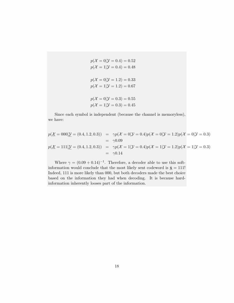
p(X = 0|Y = 0.4) = 0.52p(X = 1|Y = 0.4) = 0.48

p(X = 0|Y = 1.2) = 0.33p(X = 1|Y = 1.2) = 0.67

p(X = 0|Y = 0.3) = 0.55p(X = 1|Y = 0.3) = 0.45

Since each symbol is independent (because the channel is memoryless),we have:

p(X = 000|Y = (0.4, 1.2, 0.3)) = γp(X = 0|Y = 0.4)p(X = 0|Y = 1.2)p(X = 0|Y = 0.3)= γ0.09

p(X = 111|Y = (0.4, 1.2, 0.3)) = γp(X = 1|Y = 0.4)p(X = 1|Y = 1.2)p(X = 1|Y = 0.3)= γ0.14

Where γ = (0.09 + 0.14)−1. Therefore, a decoder able to use this soft-information would conclude that the most likely sent codeword is x = 111!Indeed, 111 is more likely than 000, but both decoders made the best choicebased on the information they had when decoding. It is because hard-information inherently looses part of the information.

18

Chapter 3

Coding theory introduction

In this chapter, we show how the set of codewords forming the code can itselfreveal the potential decoding ability of the code. How many errors can becorrected is directly dependent on how the codewords are chosen from An,the set of all words of length n. On the same time, coding theory basics arereviewed, explaining main parameters of codes, practical bounds on theseand some insights on simple codes.

3.1 What are codes?

As seen in the previous chapter, a code is the set of all the encoded words,the codewords, that an encoder can produce.

Definition 4 A q-ary code C of length n is a set of codewords in An, whereA is an alphabet of q symbols. The size of the code, noted |C|, is the numberof codewords in the code.

ExampleA ternary code of length 5 is the following set:

AAABBBABABCCCCCABCBA

The ternary alphabet used is A = A,B,C and the code size is|C| = 4 (it contains 4 codewords).

19

Codewords can be seen as vectors in the space An where the ith symbolis the ith coordinate. To compare words, the space An can be equippedwith a convenient metric called the Hamming distance.

Definition 5 The Hamming distance between two words x,y ∈ An is thenumber of coordinates in which symbols differ.

dH(x,y) = |i|xi 6= yi|

ExampledH(01110, 11000) = 3dH(BLUEBERRY,RASPBERRY ) = 4

The Hamming distance is a metric since it satisfies the triangle inequality.

dH(x,y) ≤ dH(x,w) + dH(w,y)

We invite the reader to quickly check it.

3.2 Nearest neighbor decoding

Nearest neighbor decoding is the process of decoding a received word byselecting the codeword at least Hamming distance from it. It is based onthe following theorem.

TheoremLet the channel be a memoryless symmetric one having a crossover proba-bility perr <

q−1q and assume all codewords have equal probabilities to be

sent. Under these conditions, the most likely sent codeword is the codewordat least Hamming distance from the received word.

Proof

Let y be the received word and assume that it differs in e placesfrom a codeword c. Then the probability that c was sent is:

p(X = c|Y = y) =p(c)

p(Y = y)

∏p(Yi = yi|Xi = ci).

The probability p(y) appears in each whereas p(c) is constant due to theequiprobability of the sent codeword hypothesis. Therefore, the above

20

expression is directly proportional to:∏p(Yi = yi|Xi = ci) ≤ (1− perr)n−e

(perrq − 1

)e.

Since 1− perr > 1/q and perr/(q − 1) < 1/q by hypothesis, this functionis strictly decreasing with e. Therefore, the probability that c is thesent codeword increases as e decreases so that the word being at leastHamming distance is the most likely one.

It should be kept in mind that nearest neighbor decoding is maximumlikelihood decoding under the implicit assumption that we are working witha ”normal” symmetric channel. To stress how important this assumption is,let us take a small example. Suppose the word AAXXXXB is received andeither AAXXXX or XXXXXB could be decoded. If the probability thatan A was an X before (transmission) is 1/4 and the probability that a Bwas an X before is 1/32, then it is more likely that the two A’s are erroneousthan a single B. In other words, the codeword XXXXXB would be morelikely despite it is the one having the greater distance to AAXXXXBcompared to the other codeword.

Satisfying the symmetric channel hypothesis, as well as the probabilitycondition concerning it, are crucial for nearest neighbor decoding. But thishypothesis is frequently met in practice. Either because the channel is indeeda symmetric one or because no information about likelihood of symbols isavailable to the decoder, like in hard-decoding, and thus assuming that anykind of symbol error is equiprobable. This places the hard-decoding problemin a new light. The aim of the hard decoder reduces to find the codewordat nearest distance from the received word. More formally, the most likelysent codeword x is the codeword of least distance to y.

x = argminx∈CdH(x,y)

£ Hard decoding thus forgets abouts probabilities and focuses solely onfinding the nearest codeword.

Intuitively, one can feel that it is interesting for the code to have amaximum of distance between its codewords.

Definition 6 The smallest distance between any two distinct codewords ofa code C is called the minimal distance of a code and is noted d.

d = minx,y∈C,x 6=y

dH(x,y)

21

Indeed, the minimal distance of a code is a fundamental parameter since theerror correcting ability of the code is directly related to its minimal distance.For nearest neighbor decoding, in order for the code to provide unambiguousdecoding of the received codewords up to e errors, it is necessary and suficientthat the minimal distance be at least d = 2e+ 1. This follows directly fromthe triangle inequality since no received word w can lie at distance less thanor equal to e to two codewords if they are all at a distance d = 2e+ 1.

Intuition also tells us that soft decoding performances are as well affectedby the minimal distance between codewords. However, quantifying it is adifficult task involving channel outcome probability distributions.

3.3 Space and spheres

Back to the codes. We showed that the minimal distance of a code is acrucial parameter, but what is also of interest is that it contains a maximumnumber of codewords. We will see in this section how the construction ofgood codes is equivalent to a sphere packing problem. We shall begin byconsidering the set of words at a given distance from some word and forminga Hamming sphere.

Definition 7 The Hamming sphere of radius τ around a word w is the setof all the words which are at a Hamming distance ≤ τ from w.

Hτ (w) = x ∈ An|dH(x,w) ≤ τ

ExampleConsider the alphabet A,B,C and the word AABB. The Hammingsphere of radius 2 around this word contains :

• at distance 0: AABB

• at distance 1: BABB,CABB,ABBB,ACBB,AAAB,AACB,AABA,AABC

• at distance 2: BBBB,BCBB,BAAB,BACB,BABA,BABC,CBBB,CCBB,CAAB,CACB...

Let A be an alphabet of q symbols, the number of words in a sphere ofradius τ sums up to:

22

τ∑i=0

(τi

)(q − 1)i

Hamming spheres show to be a useful concept, both by assisting under-standing and to derive bounds on code parameters. For example, requestinge errors to be unambiguously correctable is equivalent to request that theHamming spheres of radius e around any two distinct codewords do not in-tersect. Indeed, if words were in two spheres, it would mean that they areat a distance less than or equal to e from several codewords. This leads tofollowing definitions:

Definition 8 The packing radius is the greatest possible radius of spheresaround each codeword so that they do not intersect.

The covering radius is the smallest possible radius around codewords so thatany word is included in some sphere.

To get good codes, the points in space should be chosen to have thegreatest possible packing radius to maximize the minimal distance. Andon the same time, have the lowest possible covering radius to not ”wastespace”. Obviously, we always have that covering radius ≥ packing radius.Using these, it is easy to obtain lower and upper bounds on the size of acode depending of its minimal distance:

TheoremHAMMING BOUNDGiven an alphabet of size q and a space of n dimensions, the size of any codewith minimal distance 2e+ 1 is bounded from above by:

|C| ≤ qn∑ei=0

(ni

)(q − 1)i

.

Proof

This is simply the number of words in the space divided by thenumber of words in a sphere.

23

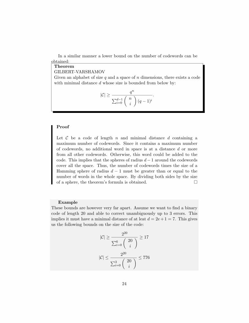
In a similar manner a lower bound on the number of codewords can beobtained:

TheoremGILBERT-VARSHAMOVGiven an alphabet of size q and a space of n dimensions, there exists a codewith minimal distance d whose size is bounded from below by:

|C| ≥ qn∑d−1i=0

(ni

)(q − 1)i

.

Proof

Let C be a code of length n and minimal distance d containing amaximum number of codewords. Since it contains a maximum numberof codewords, no additional word in space is at a distance d or morefrom all other codewords. Otherwise, this word could be added to thecode. This implies that the spheres of radius d− 1 around the codewordscover all the space. Thus, the number of codewords times the size of aHamming sphere of radius d − 1 must be greater than or equal to thenumber of words in the whole space. By dividing both sides by the sizeof a sphere, the theorem’s formula is obtained.

ExampleThese bounds are however very far apart. Assume we want to find a binarycode of length 20 and able to correct unambiguously up to 3 errors. Thisimplies it must have a minimal distance of at leat d = 2e+1 = 7. This givesus the following bounds on the size of the code:

|C| ≥ 220∑6i=0

(20i

) ≥ 17

|C| ≤ 220∑3i=0

(20i

) ≤ 776

24

And thus, we know that a code with these parameters and containing atleast 17 codewords exists, but it is impossible to find such a code containingmore than 776 codewords.

These are not the only bounds and we invite the interested reader toother resources for further informations about them. They can be found inany coding theory book such as [1] or on Wikipedia.

Achieving the Hamming bound happens when the packing radius is equalto the covering radius (why?). Codes achieving this extraordinary propertyare called perfect codes and are very scarce. These are repetition codes,Hamming codes and Golay codes. However, their parameters do not neces-sarily fit the application. Therefore, it is important to have good codes fora wide range of parameters even if they are not perfect.

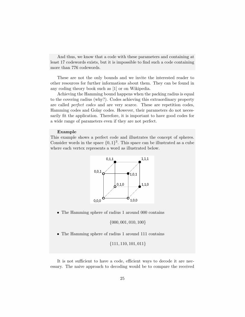
ExampleThis example shows a perfect code and illustrates the concept of spheres.Consider words in the space 0, 13. This space can be illustrated as a cubewhere each vertex represents a word as illustrated below.

• The Hamming sphere of radius 1 around 000 contains

000, 001, 010, 100

• The Hamming sphere of radius 1 around 111 contains

111, 110, 101, 011

It is not sufficient to have a code, efficient ways to decode it are nec-essary. The naive approach to decoding would be to compare the received

25

word to every codeword by measuring it’s Hamming distance. Despite thefact that this provides the best possible decoding it has unreasonable timecomplexity. For example, if there is a codeword associated to any messageof 100 bits, then this makes already more than 1030 codewords and thus asmuch comparisons. Hard-decoding paradigms can be subdivided into threecategories:

• Bounded distance decoding: this is the most frequent kind of decodingalgorithms. Given a code C and a decoding radius τ less than or equalto the packing radius (usually equal). Bounded distance decodingdecodes a received word y ∈ An to x ∈ C if dH(x,y) ≤ τ . I.e. ifthe received word lies in a sphere of radius τ around some codeword,uniquely determined. In the case the received word is in none of thespheres, a decoding failure is declared. This is why it is also referredas τ -error decoding since it decodes correctly if at most τ errors wereintroduced.

• List decoding: this problem can be seen as an extension of boundeddistance decoding. If we allow the decoding radius τ to be greater thanthe packing radius, then codewords are no more uniquely determined.List decoding therefore returns a list L = x ∈ C|dH(x,y) ≤ τ of allcodewords x ∈ C in the sphere of radius τ around the received wordy.

• Nearest codeword decoding: The decoded codeword x ∈ C is theone with the minimum distance to the received word y ∈ An. I.ex = minx∈C dH(x,y). If several codewords lie at the same distance,there is a number of options possible: the list of these codewords isreturned, a codeword is chosen at random or a failure is declared. Thisenables to correct any received words even if it lies beyond the packingradius. However, this kind of decoding turns out to be computationallydifficult in general.

In order to provide efficient encoding and decoding, it is necessary toprovide the code with some underlying structure. And for the code to bestructured, the alphabet needs some mathematical structure itself. Thisbrings us to the next chapter explaining the basics of fundamental algebraicstructures.

26

Chapter 4

Mathematics fundamentals

This chapter is devoted to covering the basic concepts of groups, rings andfields.

4.1 Groups

The most fundamental algebraic structure is a group. It satisfies the follow-ing axioms.

Definition 9 A group (G, ∗) is a set G with a binary operation ∗ : G×G→G satisfying the following 3 axioms:

• Associativity: For all a, b, c ∈ G : (a ∗ b) ∗ c = a ∗ (b ∗ c)

• Identity element: There is an element e ∈ G such that for all a ∈ G :e ∗ a = a ∗ e = a

• Inverse element: For each a ∈ G, there is an element b ∈ G such thata ∗ b = b ∗ a = e, where e is the identity element.

As is stated, a group is simply a set of elements having a neutral andinverses, noted a−1 or −a depending on the situation. A group is said to becommutative, or Abelian, if for a, b ∈ G we have ab = ba.

Example

• The set of even integers, noted 2Z is a commutative group under addi-tion. On the opposite, the set of odd integers is not a group at all sincethe sum of two odd integers does not lie in the set of odd integers.

27

• The set of invertible square matrices Rn×n forms a non-commutativegroup under multiplication where the neutral element is the identitymatrix.

• Let S be an ordered set. Consider G: the set of bijections α : S → S.That is, the elements of G are permutations of the ordered set S.The set G is a group under composition. The inverse is simply thepermutation which maps S′ to its original state and the neutral is thepermutation which does not change anything.

It is straightforward to show that the cancellation laws hold in groups:

ab = ac⇒ b = c

Since it is sufficient to premultiply both sides by a−1 to obtain the equality.Moreover the cancellation laws implies the following theorem.

TheoremThe map x→ ax : G→ G is a bijection.

Proof

To prove that the map is bijective, we will prove that it is bothinjective and surjective. The cancellation law directly implies that it isinjective since ax1 = ax2 ⇒ x1 = x2. To show surjectivity, let us showthat for every b ∈ G there exists a value for x ∈ G so that ax = b, this issimply x = a−1b.

By taking a subset of elements satisfying the properties of a group, weobtain a subgroup.

Definition 10 A subgroup (S, ∗) of (G, ∗) satisfies the following axioms:

• S ⊂ G and S 6= ∅

• if a, b ∈ S then a ∗ b ∈ S

• if a ∈ S then a−1 ∈ S

So that (S, ∗) is a group by itself with the same neutral element.

28

ExampleThe set of even integers 2Z is a subgroup of the integers Z.

By performing the operation (which can be the addition, the multiplica-tion, ...) on a subgroup by an element of a group, we obtain a coset.

Definition 11 Let (H, ∗, e) be a subgroup of (G, ∗, e), both commutative. Acoset of H in G is a set of the form

aH = ah|h ∈ H = Ha

for some fixed a ∈ G.

ExampleLet us take as group the integers Z under addition. Then 5Z is a subgroupof it and 5Z + 1 is a coset.

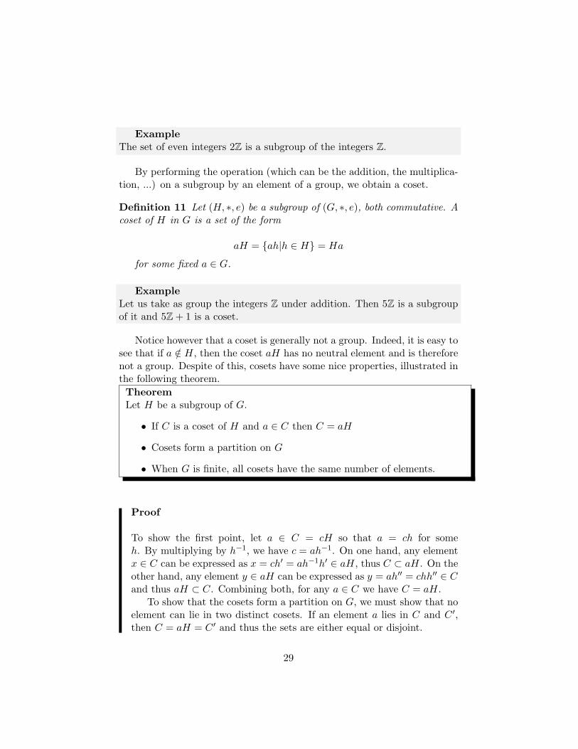
Notice however that a coset is generally not a group. Indeed, it is easy tosee that if a /∈ H, then the coset aH has no neutral element and is thereforenot a group. Despite of this, cosets have some nice properties, illustrated inthe following theorem.

TheoremLet H be a subgroup of G.

• If C is a coset of H and a ∈ C then C = aH

• Cosets form a partition on G

• When G is finite, all cosets have the same number of elements.

Proof

To show the first point, let a ∈ C = cH so that a = ch for someh. By multiplying by h−1, we have c = ah−1. On one hand, any elementx ∈ C can be expressed as x = ch′ = ah−1h′ ∈ aH, thus C ⊂ aH. On theother hand, any element y ∈ aH can be expressed as y = ah′′ = chh′′ ∈ Cand thus aH ⊂ C. Combining both, for any a ∈ C we have C = aH.

To show that the cosets form a partition on G, we must show that noelement can lie in two distinct cosets. If an element a lies in C and C ′,then C = aH = C ′ and thus the sets are either equal or disjoint.

29

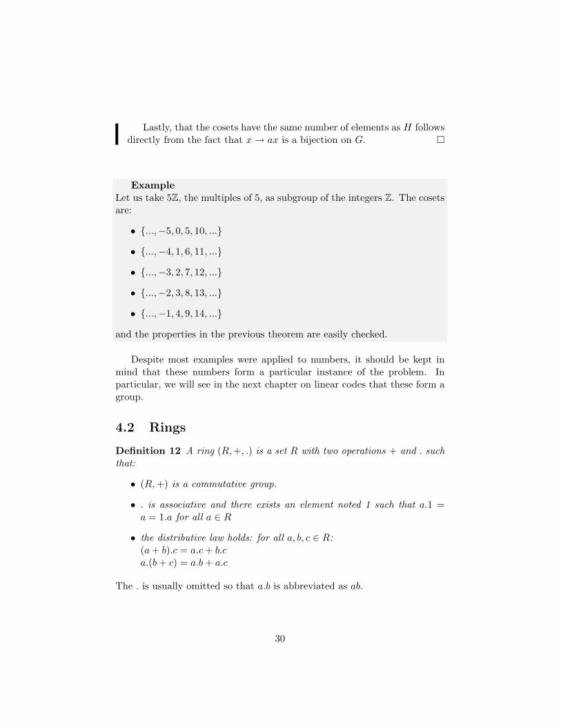
Lastly, that the cosets have the same number of elements as H followsdirectly from the fact that x→ ax is a bijection on G.

ExampleLet us take 5Z, the multiples of 5, as subgroup of the integers Z. The cosetsare:

• ...,−5, 0, 5, 10, ...

• ...,−4, 1, 6, 11, ...

• ...,−3, 2, 7, 12, ...

• ...,−2, 3, 8, 13, ...

• ...,−1, 4, 9, 14, ...

and the properties in the previous theorem are easily checked.

Despite most examples were applied to numbers, it should be kept inmind that these numbers form a particular instance of the problem. Inparticular, we will see in the next chapter on linear codes that these form agroup.

4.2 Rings

Definition 12 A ring (R,+, .) is a set R with two operations + and . suchthat:

• (R,+) is a commutative group.

• . is associative and there exists an element noted 1 such that a.1 =a = 1.a for all a ∈ R

• the distributive law holds: for all a, b, c ∈ R:(a+ b).c = a.c+ b.ca.(b+ c) = a.b+ a.c

The . is usually omitted so that a.b is abbreviated as ab.

30

ExampleThe integers Z form a ring whereas the set of even numbers 2Z is not a ring.Checking this using the definition is left as a small exercise for the reader.

The most frequent example of rings is modular arithmetic, sometimesalso called ”clock arithmetic” and works as follows. Two integers a, b arecongruent modulo n if and only if a− b is a multiple of n.

a ≡ b (mod n) ⇔ n|(a− b)

The notation on the right means n divides a − b. Such a ring is notedZ/nZ. The sets of congruent integers form n equivalence classes partitioningZ.

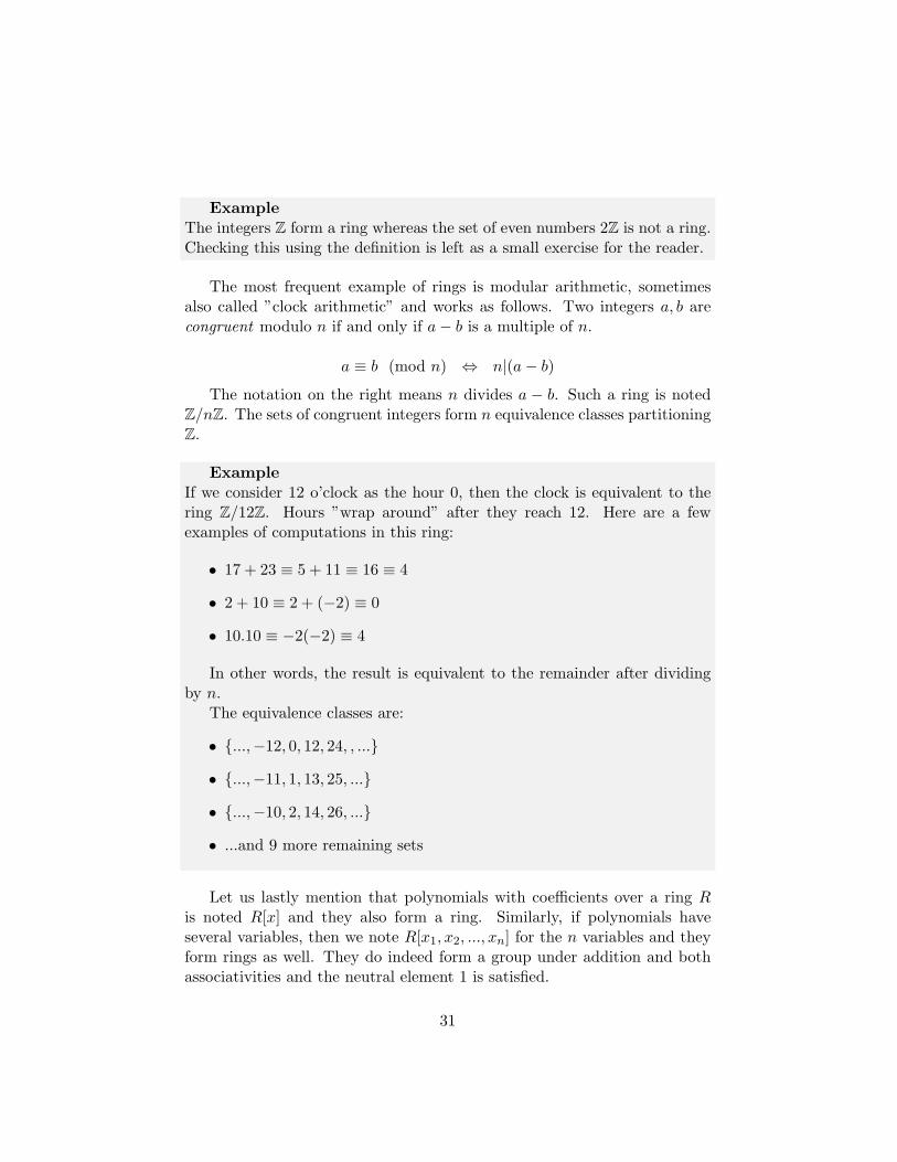
ExampleIf we consider 12 o’clock as the hour 0, then the clock is equivalent to thering Z/12Z. Hours ”wrap around” after they reach 12. Here are a fewexamples of computations in this ring:

• 17 + 23 ≡ 5 + 11 ≡ 16 ≡ 4

• 2 + 10 ≡ 2 + (−2) ≡ 0

• 10.10 ≡ −2(−2) ≡ 4

In other words, the result is equivalent to the remainder after dividingby n.

The equivalence classes are:

• ...,−12, 0, 12, 24, , ...

• ...,−11, 1, 13, 25, ...

• ...,−10, 2, 14, 26, ...

• ...and 9 more remaining sets

Let us lastly mention that polynomials with coefficients over a ring Ris noted R[x] and they also form a ring. Similarly, if polynomials haveseveral variables, then we note R[x1, x2, ..., xn] for the n variables and theyform rings as well. They do indeed form a group under addition and bothassociativities and the neutral element 1 is satisfied.

31

However, they do not behave like in usual arithmetics, for example divi-sion is not always possible and a polynomial could factor several ways. Forexample, in (Z/6Z)[x], we have:

(x+ 2)(x+ 3) ≡ x2 + 5x ≡ x(x+ 5)

This motivates the need of a stronger algebraic structure.

4.3 Fields

Fields are mathematical structures behaving with the same rules as usualarithmetic and close to our everyday intuition. A field is a set where opera-tions like addition, subtraction, multiplication or division subject to the lawsof commutativity, distributivity, associativity and other ”usual” properties.

Definition 13 A field is a set F or F with two operations + and . suchthat:

• (F,+) is a commutative group;

• (F ∗, .), where F ∗ = F \ 0, is a commutative group;

• the distributive law holds.

Notice that a field is a ring, by definition, with the additional propertythat every element has an inverse under multiplication. Some common ex-amples of fields are R, C and Q. Indeed, every axiom is straightforward toverify. However, the set of integers Z is not a field. Indeed, for (Z∗, .) to be agroup, any of its element should have an inverse under multiplication. Thisis clearly not the case since no integers have an inverse in this set except −1and 1.

Moreover, it should be noted that no flat assumptions are made aboutoperations like subtraction or division. These two can respectively be seenas undoing the operation, i.e. a+ (−b) and a.b−1. Other familiar propertiesare not assumed by default but easily proved.

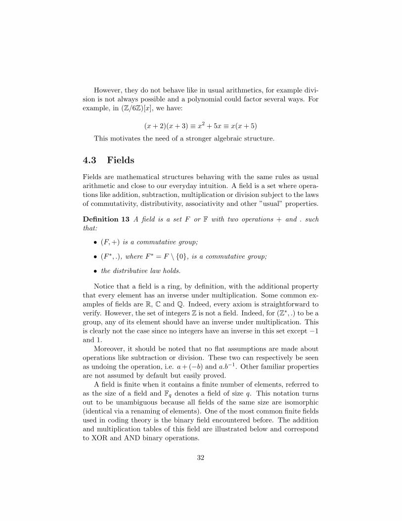
A field is finite when it contains a finite number of elements, referred toas the size of a field and Fq denotes a field of size q. This notation turnsout to be unambiguous because all fields of the same size are isomorphic(identical via a renaming of elements). One of the most common finite fieldsused in coding theory is the binary field encountered before. The additionand multiplication tables of this field are illustrated below and correspondto XOR and AND binary operations.

32

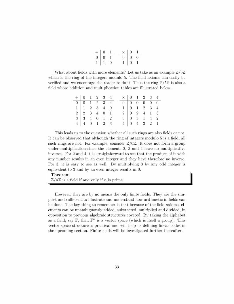
+ 0 10 0 11 1 0

× 0 10 0 01 0 1

What about fields with more elements? Let us take as an example Z/5Zwhich is the ring of the integers modulo 5. The field axioms can easily beverified and we encourage the reader to do it. Thus the ring Z/5Z is also afield whose addition and multiplication tables are illustrated below.

+ 0 1 2 3 40 0 1 2 3 41 1 2 3 4 02 2 3 4 0 13 3 4 0 1 24 4 0 1 2 3

× 0 1 2 3 40 0 0 0 0 01 0 1 2 3 42 0 2 4 1 33 0 3 1 4 24 0 4 3 2 1

This leads us to the question whether all such rings are also fields or not.It can be observed that although the ring of integers modulo 5 is a field, allsuch rings are not. For example, consider Z/6Z. It does not form a groupunder multiplication since the elements 2, 3 and 4 have no multiplicativeinverses. For 2 and 4 it is straightforward to see that the product of it withany number results in an even integer and they have therefore no inverse.For 3, it is easy to see as well. By multiplying 3 by any odd integer isequivalent to 3 and by an even integer results in 0.

TheoremZ/nZ is a field if and only if n is prime.

However, they are by no means the only finite fields. They are the sim-plest and sufficient to illustrate and understand how arithmetic in fields canbe done. The key thing to remember is that because of the field axioms, el-ements can be unambiguously added, subtracted, multiplied and divided, inopposition to previous algebraic structures covered. By taking the alphabetas a field, say F, then Fn is a vector space (which is itself a group). Thisvector space structure is practical and will help us defining linear codes inthe upcoming section. Finite fields will be investigated further thereafter.

33

Chapter 5

Linear codes

5.1 Definition

An important family of codes is linear codes. They do not only admitsimple representations but also have practical reasons by providing efficienttechniques of encoding and decoding.

Definition 14 Let F be a field. A linear code is a vector subspace of Fn:

∀a, b ∈ F, ∀x,y ∈ C : ax + by ∈ C

ExampleOver F3, the following code is linear:000001110022200001110022211211220111102222122

Indeed, any linear combination of codewords is also a codeword.

Since a linear code is a vector subspace, a convenient way to express itis by means of a basis of this subspace. This is the role of the generatormatrix.

34

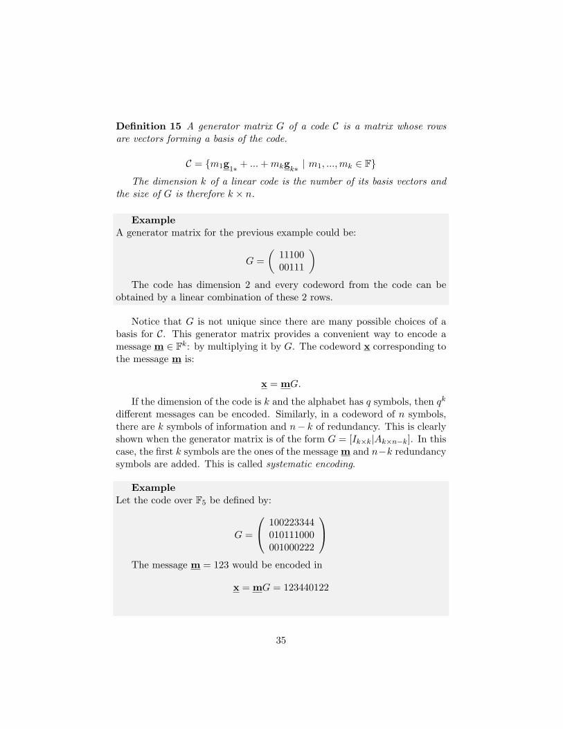
Definition 15 A generator matrix G of a code C is a matrix whose rowsare vectors forming a basis of the code.

C = m1g1∗ + ...+mkgk∗ | m1, ...,mk ∈ F

The dimension k of a linear code is the number of its basis vectors andthe size of G is therefore k × n.

ExampleA generator matrix for the previous example could be:

G =(

1110000111

)The code has dimension 2 and every codeword from the code can be

obtained by a linear combination of these 2 rows.

Notice that G is not unique since there are many possible choices of abasis for C. This generator matrix provides a convenient way to encode amessage m ∈ Fk: by multiplying it by G. The codeword x corresponding tothe message m is:

x = mG.

If the dimension of the code is k and the alphabet has q symbols, then qk

different messages can be encoded. Similarly, in a codeword of n symbols,there are k symbols of information and n− k of redundancy. This is clearlyshown when the generator matrix is of the form G = [Ik×k|Ak×n−k]. In thiscase, the first k symbols are the ones of the message m and n−k redundancysymbols are added. This is called systematic encoding.

ExampleLet the code over F5 be defined by:

G =

100223344010111000001000222

The message m = 123 would be encoded in

x = mG = 123440122

35

The counterpart of the generator matrix is the parity matrix H.

Definition 16 A parity matrix H of a code C is a matrix whose rows arevectors forming a basis of the nullspace of the code.

C = c ∈ Fn|HcT = 0

If the code has dimension k then the dimension of its nullspace is n− k andthe size of H is therefore (n− k)× n.

And here again H is not unique. Since the rows of H form a basis of thenullspace of the code whose basis is the rows of G, we have:

GHT = HGT = 0

Notice that the roles of G and H are invertible. This leads to the notionof dual code.

Definition 17 The dual of a code C defined by a generator matrix G is thecode C⊥ whose parity matrix is G. Similarly, if H is the parity matrix of Cthen H is the generator matrix of C⊥.

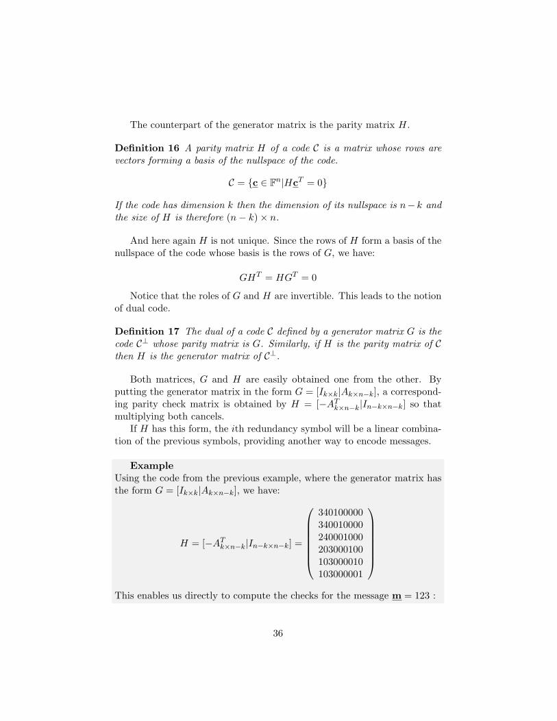
Both matrices, G and H are easily obtained one from the other. Byputting the generator matrix in the form G = [Ik×k|Ak×n−k], a correspond-ing parity check matrix is obtained by H = [−ATk×n−k|In−k×n−k] so thatmultiplying both cancels.

If H has this form, the ith redundancy symbol will be a linear combina-tion of the previous symbols, providing another way to encode messages.

ExampleUsing the code from the previous example, where the generator matrix hasthe form G = [Ik×k|Ak×n−k], we have:

H = [−ATk×n−k|In−k×n−k] =

340100000340010000240001000203000100103000010103000001

This enables us directly to compute the checks for the message m = 123 :

36

• x3 = −3x1 − 4x2 = 4

• x4 = −3x1 − 4x2 = 4

• x5 = −2x1 − 4x2 = 0

• ...

And we obtain the same codeword x = 123440122 (of course!) whichsatisfies Hx = 0.

As a summary, we can write:

C = Im(G) = Ker(H)

Lastly, let us mention that the analogy with vector spaces on fields ofcharacteristic zero like the reals R stops here. For example, the scalar prod-uct of a vector by itself can give zero. In other words, the vector is orthogonalto itself. This can of course be extended to a set of vectors and lead to theinteresting case of selfdual codes. These codes have the interesting propertythat their generator and parity check matrices are identical.

ExampleThe following code over the binary field is selfdual:

G =(

11000011

)= H

It is easy to verify that:

GHT = HGT = 0

To summarize it, a code is characterized by four important parameters:

• its alphabet

• its length n

• its dimension k

• its minimal distance d

37

And a code is sometimes noted with parameters in brackets and has theform C[n, k, d].

Determining its minimal distance can be done several ways.

Definition 18 The Hamming weight of a word w ∈ An is the number ofnon-null symbols the word contains.

wH(w) = dH(0,w)

And using this definition, we can show that the minimal distance of a linearcode is equal to the minimum weight of its nonzero codewords.

d = min06=c∈C

wH(c)

If there were two codewords, say x and y so that dH(x,y) < d, thenx − y would also be in the code and have a Hamming weight less than dwhich contradicts the hypothesis that we took d as the minimum weight.

For linear codes, one of the most fundamental bounds is the SingletonBound which combines the three main parameters k, n and d as follows.

d ≤ n− k + 1

It can be explained two ways. Given a code C[n, k, d], if all codewordsare projected on k−1 coordinates, then (since there are qk codewords) somecodewords must agree on all these k−1 coordinates. Thus, these codewordsthen disagree on at most all other coordinates, i.e. the minimal distance isat most n− (k − 1) proving the inequality.

The other way to show the bound makes use of H. For any set oflinearly dependent columns of H, there exists a codeword acting on thesewhose weight is equal to the size of this set. Thus, the minimal weightof codewords (=d) is equal to the minimum number of linearly dependentcolumns. Since any set of n− k + 1 columns are necessarily dependent thisgives an upper bound on the minimum size of such a set and the aboveinequality is obtained. Codes achieving this bound are called maximumdistance separable codes.

5.2 Hard decoding using the syndrome

Let x be the sent codeword and let y be the received word. Since we areworking in Fnq , the error vector can be expressed as e = y − x. The error

38

vector e is 0 in the locations where the channel did not introduce errors andnonzero where errors were introduced. By definition, we have:

y = x + e.

Since a linear code is a vector subspace, it is also a subgroup of Fn.By adding the error vector, y falls in the coset C + e and all cosets form apartition over Fn. Taking this the other way round, we know that given areceived vector y, the error vector lies in the coset C + y. The most likelyerror vector is then a word of least weight in this coset and is called cosetleader. If it is unique, nearest neighbor decoding is unambiguous, else, thereare several error vectors of same weight to choose from.

ExampleLet the linear code C over F2 be defined by:

G =(

11111000011111

)If the received vector is 1110000 we know that the error is in the coset

formed by1110000, 0001100, 1101111, 0010011

so that the most likely error is 0001100 and results in the decoded codeword1111100. It is nevertheless possible that more errors were introduced so thatthis choice would be the wrong one and another word of the coset be thecorrect error word. However, taking the most likely error word, i.e. thecoset leader, remains the best choice that can be made.

A nice relationship with the Hamming spheres can be shown. The pack-ing radius is the maximum value so that any coset leader having a weightless than or equal to this radius is unique. The covering radius on the otherhand is equal to the maximum weight of any coset leader.

ExampleIn the previous example, there are 25 = 32 cosets:

• 7 cosets with unique coset leaders of weight 1.

• 19 cosets with unique coset leaders of weight 2.

• 1 coset with 2 coset leaders of weight 2, 1100000, 0000011

39

• 5 cosets with several coset leaders of weight 3.

This means that unambiguous decoding can take place for any singleerror as well as in 19 of 21 cases of double errors. There 2 double errorswhere 2 most likely decoded codewords are possible. The packing radius is1 and the covering radius is 3.

Here comes a general decoding technique. Let C + y be the coset towhich the received word belong. Since the sent codeword x is not knowna priori, the most likely error e is the coset leader of C + y and we havex = y − e. Thus a way to identify cosets is needed as well as a dictionarymapping the cosets to one of their respective coset leader, having thereforeqn−k entries.

A way to identify cosets is the syndrome.

Definition 19 The syndrome s of a received word y is:

s = yHT .

Like in medical terminology where a syndrome means a pattern of symp-toms helping to identify a disease, the syndrome in coding theory can beused as a unique coset identifier. This fact is illustrated by the followingproperty:

s = yHT = xHT + eHT = eHT .

This formula shows that the syndrome is the same for any words of a samecoset. The codewords are ”filtered out” so that only the error word affectsthe syndrome. This provides a straightforward way to make a syndromedictionary : a lookup table mapping syndromes to their corresponding cosetleader, i.e. the most likely error word.

ExampleLet a linear code C over F5 be defined by the following parity check matrix:

H =(

011111101234

)It can correct up to one error since any two columns are independent.

The code size would be 54 = 625 which is also the size of the cosets. There-fore, a naive decoder would need 625 comparaisons. On the opposite, thereare 52 = 25 cosets that can already be associated with a coset leader:

40

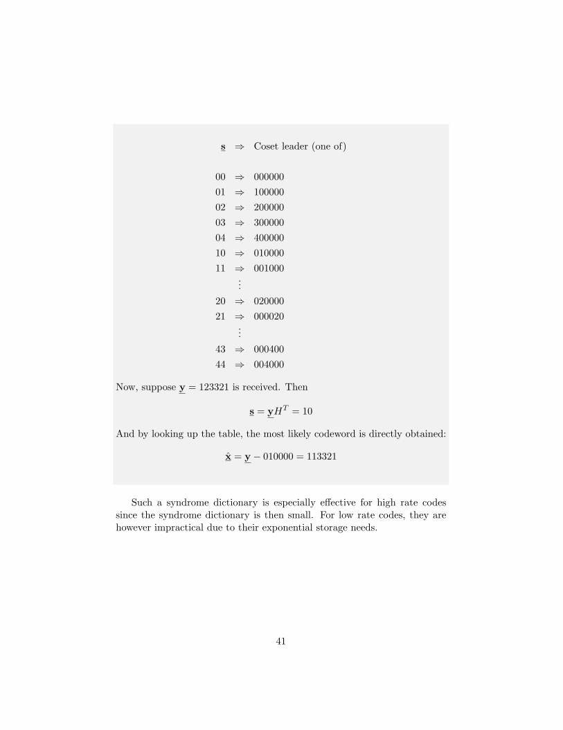
s ⇒ Coset leader (one of)

00 ⇒ 00000001 ⇒ 10000002 ⇒ 20000003 ⇒ 30000004 ⇒ 40000010 ⇒ 01000011 ⇒ 001000

...20 ⇒ 02000021 ⇒ 000020

...43 ⇒ 00040044 ⇒ 004000

Now, suppose y = 123321 is received. Then

s = yHT = 10

And by looking up the table, the most likely codeword is directly obtained:

x = y − 010000 = 113321

Such a syndrome dictionary is especially effective for high rate codessince the syndrome dictionary is then small. For low rate codes, they arehowever impractical due to their exponential storage needs.

41

Chapter 6

More on fields

A few chapters before, fields were briefly introduced. It is now time to coverthem more in depth. The aims of this section are multiple. First, to explainbasic proprieties of fields to become familiar with them, then to reviewpolynomial arithmetic over fields and lastly how to construct extension fieldsof a given field.

6.1 Field properties

Let us take an element a 6= 0 ∈ F, where F is finite. By taking the seriesa+ a, a+ a+ a, ... there is a point where it will come back to zero and wraparound. If it was not, we would have that two different sums of a’s wouldbe equal since the field is finite. Thus the difference of them, also a sum ofa’s, would be zero leading to the same conclusion. Since the element can beput in evidence, it boils down to knowing how many times 1, the neutralunder multiplication, can be added to itself before wrapping to zero sincethe same applies to any element of F, forming cyclic subgroups of F.

Definition 20 The characteristic of a finite field Fq is the smallest integerp such that

1 + 1 + ...+ 1︸ ︷︷ ︸p times

= 0

The characteristic of a finite field is a prime number. Otherwise there wouldbe divisors of zero, i.e. some a 6= 0, b 6= 0 ∈ Fq so that ab = 0. Bymultiplying by a−1 we have that b = 0 which contradicts our hypothesis.

42

TheoremThe size of a finite field is a power of a prime.

Proof

Suppose p is the characteristic of the field Fq with q > p. Take amaximal set of elements β1, β2, ..., βm in Fq which are linearly inde-pendent over Fp. That is, no two two sums of β’s can be equal. Thenthe field contains, by closure, any linear combination of them.

α1β1 + α2β2 + ...+ αmβm ∈ Fq

And no others. Fq is a vector space of dimension m over Fp and has thusq = pm elements.

Of course, multiplication must be defined on this vector space in orderto provide the structure of a field. It turns out that all fields of same sizeare isomorphic. That fields of same size are isomorphic means that one canbe obtained from another simply by renaming the elements. This enablesus to write Fq without ambiguity. Before we show how to construct fieldswhose sizes are powers of a prime, a little introduction about polynomialsover fields is necessary. In opposition to polynomials over rings, polynomialsover fields have a unique factorization.

Definition 21 A polynomial p(x) in F[x] is called irreducible over the fieldF if it is non-constant and cannot be represented as the product of two non-constant polynomials from F[x].

ExampleThe polynomial x2 + 1 is irreducible over F3 but not over F2 where we havex2 + 1 = (x+ 1)2.

The concept of modular arithmetic can be generalized to polynomialsover fields. Then F[x]/p(x) where p(x) ∈ F[x] becomes a set equivalenceclasses of polynomials.

TheoremThe equivalence classes Fq[x]/r(x) form a field of size qdeg(r(x)) if and onlyif r(x) ∈ Fq[x] is an irreducible polynomial.

43

The proof is similar to the one of APPENDIX A.1.

Definition 22 The order of a non-zero element a ∈ Fq is the smallestinteger m > 0 so that am = 1.

For every finite field Fq there exists an element of order q − 1 which iscalled a primitive element. Thus, a finite field is composed of zero and allq − 1 powers of this primitive element. This in turn means that F∗q forms acyclic group under multiplication whose generator is the primitive element.

ExampleLet us take the irreducible polynomial r(x) = x3 + x + 1 over F2. Saidin another way, we have x3 = x + 1. Then we have, along with differentrepresentations:

0 ⇔ 000 ⇔ 01 ⇔ 100 ⇔ 1α ⇔ 010 ⇔ 2α2 ⇔ 001 ⇔ 4α3 = α+ 1 ⇔ 110 ⇔ 3α4 = α2 + α ⇔ 011 ⇔ 6α5 = α2 + α+ 1 ⇔ 111 ⇔ 7α6 = α2 + 1 ⇔ 101 ⇔ 5... (α7 = 1)

This set forms F23 and α is a primitive element.

The irreducible polynomial in the example above is special since theprimitive element is a root of it. Such a polynomial is called a primitivepolynomial.

Since F∗q is a cyclic group of order q−1, we have the interesting propertythat βq = β for all β ∈ F ∗q . Therefore, every β ∈ Fq is a root of xq − x,giving rise to the following factorization:

xq − x =∏β∈Fq

(x− β)

6.2 The extended Euclidean algorithm

We present an important algorithm which will be of later use in decodingspecific codes. This algorithm is very general and not limited to finite fields.It computes the smallest common divisor of a pair of integers or a pair of

44

polynomials in one variable. For simplicity, we explain it here by applyingit on a pair of integers.

The algorithm works by decomposing every number in smaller and smallersubparts by means of divisions with quotient and remainder. Suppose wewant to compute the greatest common divisor of, say, r0 and r1, with r1 < r0.This is denoted by gcd(r0, r1). We will proceed by scrambling these twonumbers into smaller and smaller pieces until we obtain a divisor of both.Here is how to proceed:

r0 = q1r1 + r2 with r2 < r1

r1 = q2r2 + r3 with r2 < r1

...rm−1 = qmrm + 0 with rm+1 = 0

Or, shortly, we perform:

ri−1 = qiri + ri+1 with ri+1 < ri, 1 ≤ i ≤ m

until rm+1 = 0. That the algorithm is guaranteed to stop is straightforwardsince the remainders ri are strictly decreasing at each iteration. To showthat the last non-zero remainder rm is the greatest common divisor of r0

and r1, we must proceed by induction. Since ri−1 can be expressed by alinear combination of ri and ri+1, we have, by induction, that r0 and r1 canboth be expressed by a linear combination of rm and rm+1 also. And, sincethe latter one is null, both r0 and r1 can be expressed as multiples of rmsolely.

ExampleLet us compute gcd(654, 123) over the integers. We have:

654 = 5.123 + 39123 = 3.39 + 639 = 6.6 + 36 = 2.3 + 0

And thus gcd(654, 123) = 3 where 654 = 214.3 and 123 = 41.3. Duringthe process above, notice that the upper divisors and remainders can alwaysbe replaced by a sum of ”smaller ones”. For example, 654 = 5.(3.39+6)+39,then replace 39 by smaller ones and so on until at some time, everythingboils down to a multiple 3.

45

The extended Euclidean algorithm provides an additional side computa-tion to find the ring elements u and v satisfying Bezout’s identity:

gcd(a, b) = ua+ vb

Over the integers, either u or v is obviously negative. It works hand inhand with the basic Euclidean algorithm. Notice that the remainders, asusual with ri+1 < ri, can be expressed as follows:

ri+1 = ri−1 − qiriAnd thus, rm can be expressed, by induction, as a sum of multiples of

r0 and r1. A practical way to keep track of the values u and v is to computethem iteratively at each step of the basic Euclidean algorithm so that:

ri = uir0 + vir1

Thus, at each step, ui and vi must be updated as follows:

ui+1 = ui−1 − q1ui vi+1 = vi−1 − q1vi,

with the initial values u0 = 1, u1 = 0, v0 = 0, v1 = 1.

ExampleLet us compute gcd(654, 123) over the integers along with the values of uiand vi at each step.

i ri qi ui vi0 654 / 1 01 123 5 0 12 39 3 1 −53 6 6 −3 164 3 2 19 −101

And the relation ri = uir0 + vir1 can be verfied at each step. Another wayto make apparent the computation of the ui and vi is the following:

39 = 654− 5.1236 = 123− 3.39

= 3(654− 5.123)= −3.654 + 16.123

3 = 39− 6.6= (654− 5.123)− 6(−3.654 + 16.123)= 19.654− 101.123

46

Lastly, note that despite the examples were taken with integers, thealgorithm is much more general. It can be applied over various algebraicstructures and in particular to polynomials over fields. This will be used fora decoding technique in the next chapter.

47

Chapter 7

Reed-Solomon codes

In 1960, I.S. Reed and G. Solomon introduced a family of error-correcting codes that are doubly blessed. The codes and theirgeneralizations are useful in practice, and the mathematics thatlies behind them is interesting.

J. Hall - lecture notes

Reed-Solomon codes, abbreviated RS codes, are designed by oversam-pling a polynomial constructed from the data. The message to send ismapped to a polynomial and the codeword is defined by evaluating it atseveral points.

Definition 23 Generalized Reed-Solomon codeLet α = (α1, ..., αn) be the locations where the Generalized Reed-Solomoncode is evaluated, with αi 6= αj for all i 6= j. Let λ = (λ1, ..., λn) be thenon-zero normalizing coefficients. Then, the GRS(n,k,α,λ) code is defined asthe set of codewords:

(λ1f(α1), λ2f(α2), ..., λnf(αn))|f(x) ∈ Fq[x] with deg(f(x)) < k

A classic Reed-Solomon code is the same without the normalizing coef-ficients which constitute the ”generalization”. The RS code is obtained byevaluating polynomials of degree less than k at n different locations αi. Thenormalizing coefficients of a GRS code have a less important role since theysimply rescale values at each location by a given factor λi. Such a GRScode can also be represented by a generator matrix of the type:

48

G =

1 1 ... 1

λ1α1 λ2α2 ... λnαnλ1α

21 λ2α

22 ... λnα

2n

......

...λ1α

k−11 λ2α

k−12 ... λnα

k−1n

However, it is sometimes more convenient to think in terms of polynomi-

als. Let m = (m0, ...,mk−1) ∈ Fkq be the message to send. Consider now thebijection to f(x) = m0 + m1x + ... + mk−1x

k−1. This polynomial is calledthe encoding polynomial. The codeword is then constructed by evaluatingthis polynomial at the predefined positions α = (α1, ..., αn). The codewordis c = (λ1f(α1), λ2f(α2), ..., λnf(αn)).

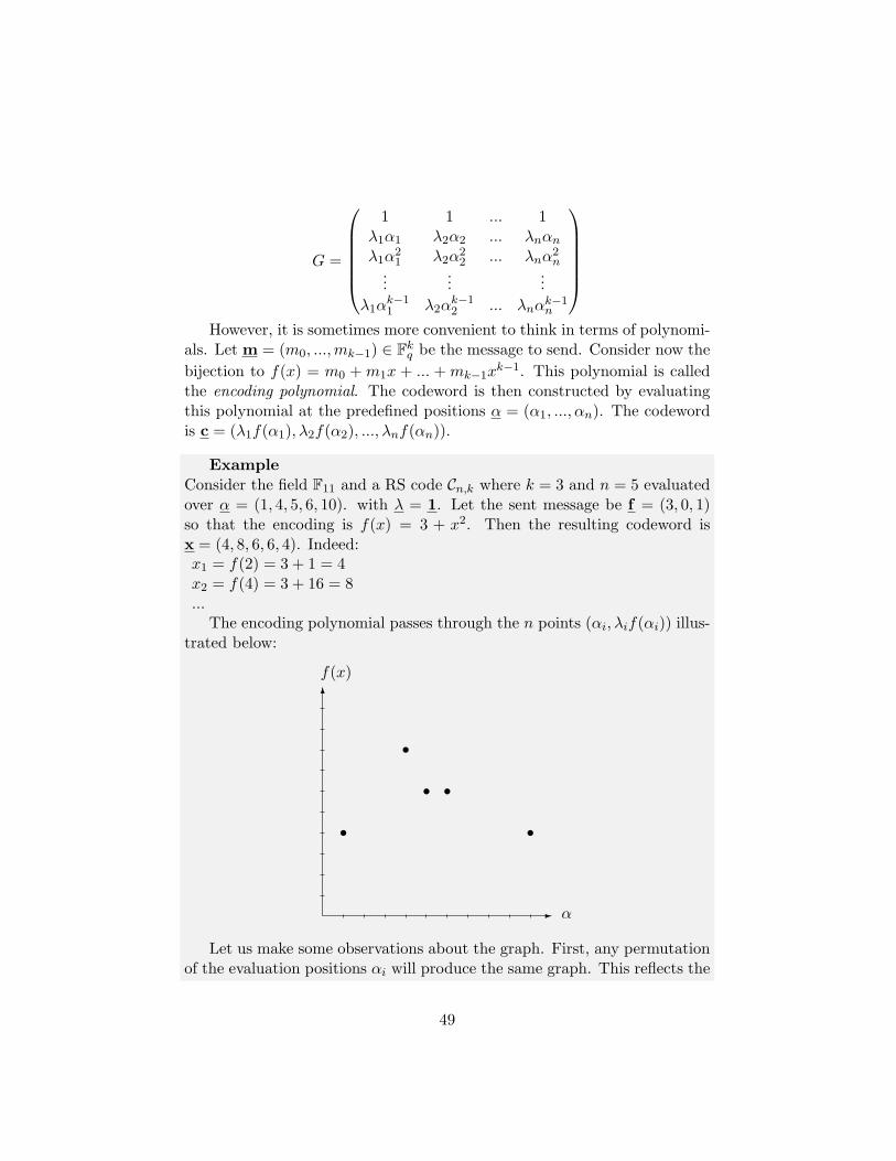
ExampleConsider the field F11 and a RS code Cn,k where k = 3 and n = 5 evaluatedover α = (1, 4, 5, 6, 10). with λ = 1. Let the sent message be f = (3, 0, 1)so that the encoding is f(x) = 3 + x2. Then the resulting codeword isx = (4, 8, 6, 6, 4). Indeed:x1 = f(2) = 3 + 1 = 4x2 = f(4) = 3 + 16 = 8...

The encoding polynomial passes through the n points (αi, λif(αi)) illus-trated below:

-

6

α

f(x)

s

ss s

s

Let us make some observations about the graph. First, any permutationof the evaluation positions αi will produce the same graph. This reflects the

49

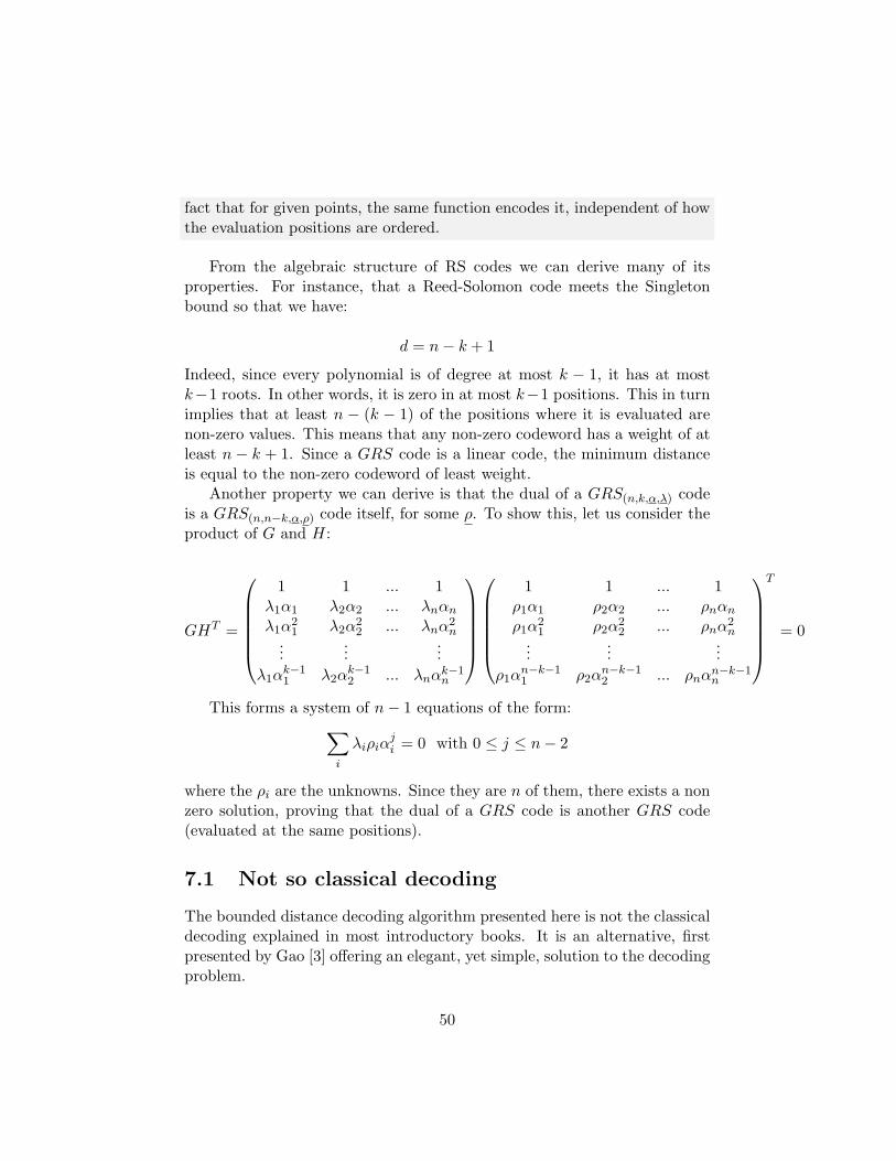
fact that for given points, the same function encodes it, independent of howthe evaluation positions are ordered.

From the algebraic structure of RS codes we can derive many of itsproperties. For instance, that a Reed-Solomon code meets the Singletonbound so that we have:

d = n− k + 1

Indeed, since every polynomial is of degree at most k − 1, it has at mostk−1 roots. In other words, it is zero in at most k−1 positions. This in turnimplies that at least n − (k − 1) of the positions where it is evaluated arenon-zero values. This means that any non-zero codeword has a weight of atleast n − k + 1. Since a GRS code is a linear code, the minimum distanceis equal to the non-zero codeword of least weight.

Another property we can derive is that the dual of a GRS(n,k,α,λ) codeis a GRS(n,n−k,α,ρ) code itself, for some ρ. To show this, let us consider theproduct of G and H:

GHT =

1 1 ... 1

λ1α1 λ2α2 ... λnαnλ1α

21 λ2α

22 ... λnα

2n

......

...λ1α

k−11 λ2α

k−12 ... λnα

k−1n

1 1 ... 1

ρ1α1 ρ2α2 ... ρnαnρ1α

21 ρ2α

22 ... ρnα

2n

......

...ρ1α

n−k−11 ρ2α

n−k−12 ... ρnα

n−k−1n

T

= 0

This forms a system of n− 1 equations of the form:∑i

λiρiαji = 0 with 0 ≤ j ≤ n− 2

where the ρi are the unknowns. Since they are n of them, there exists a nonzero solution, proving that the dual of a GRS code is another GRS code(evaluated at the same positions).

7.1 Not so classical decoding

The bounded distance decoding algorithm presented here is not the classicaldecoding explained in most introductory books. It is an alternative, firstpresented by Gao [3] offering an elegant, yet simple, solution to the decodingproblem.

50

TheoremGAO DECODING ALGORITHMInput: the received word y = (y1, ..., yn) ∈ FnqOutput: the encoding polynomial f(z) or ”Decoding failure”

• Step 1: Set p0(z) =∏ni=1(z − αi) and find the (unique) polynomial

p1(z) of degree n− 1 such that p1(αi) = yi for i = 1, ..., n.

• Step 2: Apply the extended euclidean algorithm on p0 and p1 and stopwhen the remainder pm(z) has degree less than n+k

2 .

• Step 3: Perform the division pm(z) = f(z)vm(z) + r(z). If r(z) = 0and deg(f(z)) < k then output f(z) as the encoding polynomial, elsedeclare a ”Decoding failure”.

Proof

In the following proof, we assume that e errors were introduced.

e = |i|f(αi) 6= yi|

Letw(z) =

∏i

(z − αi) , i|f(αi) = yi

w(z) =∏i

(z − αi) , i|f(αi) 6= yi

Let us moreover define the polynomial ∆(z) of degree at most e− 1 suchthat:

∆(αi) =yi − f(αi)w(αi)

, i|f(αi) 6= yi

Since there are e constraints and deg(∆(z)) ≤ e − 1, this polynomialexists and is unique. In order to make the proof lighter and the readingeasier, the variable will be hidden by default so that f is directly writteninstead of f(z) and so on. Using these polynomials, both p0 and p1 canbe expressed as follows:

p0 =n∏i=1

(z − αi) = ww

51

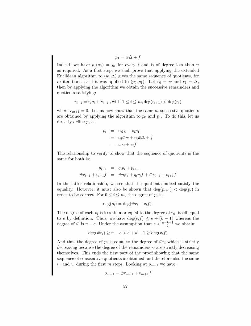
p1 = w∆ + f

Indeed, we have p1(αi) = yi for every i and is of degree less than nas required. As a first step, we shall prove that applying the extendedEuclidean algorithm to (w,∆) gives the same sequence of quotients, form iterations, as if it was applied to (p0, p1). Let r0 = w and r1 = ∆,then by applying the algorithm we obtain the successive remainders andquotients satisfying:

ri−1 = riqi + ri+1 ,with 1 ≤ i ≤ m,deg(ri+1) < deg(ri)

where rm+1 = 0. Let us now show that the same m successive quotientsare obtained by applying the algorithm to p0 and p1. To do this, let usdirectly define pi as:

pi = uip0 + vip1

= uiww + viw∆ + f

= wri + vif

The relationship to verify to show that the sequence of quotients is thesame for both is:

pi−1 = qipi + pi+1

wri−1 + vi−1f = wqiri + qivif + wri+1 + vi+1f

In the latter relationship, we see that the quotients indeed satisfy theequality. However, it must also be shown that deg(pi+1) < deg(pi) inorder to be correct. For 0 ≤ i ≤ m, the degree of pi is:

deg(pi) = deg(wri + vif).

The degree of each vi is less than or equal to the degree of r0, itself equalto e by definition. Thus, we have deg(vif) ≤ e + (k − 1) whereas thedegree of w is n− e. Under the assumption that e < n−k+1

2 we obtain:

deg(wri) ≥ n− e > e+ k − 1 ≥ deg(vif)

And thus the degree of pi is equal to the degree of wri which is strictlydecreasing because the degree of the remainders ri are strictly decreasingthemselves. This ends the first part of the proof showing that the samesequence of consecutive quotients is obtained and therefore also the sameui and vi during the first m steps. Looking at pm+1 we have:

pm+1 = wrm+1 + vm+1f

52

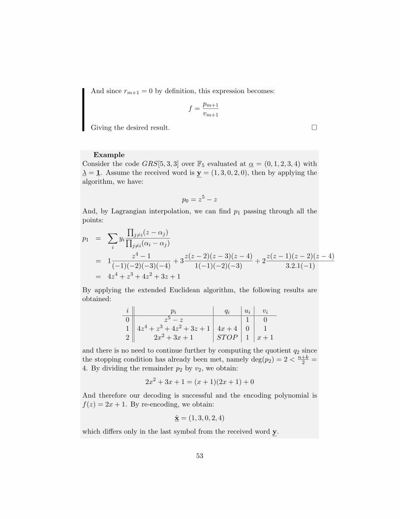
And since rm+1 = 0 by definition, this expression becomes:

f =pm+1

vm+1

Giving the desired result.

ExampleConsider the code GRS[5, 3, 3] over F5 evaluated at α = (0, 1, 2, 3, 4) withλ = 1. Assume the received word is y = (1, 3, 0, 2, 0), then by applying thealgorithm, we have:

p0 = z5 − zAnd, by Lagrangian interpolation, we can find p1 passing through all thepoints:

p1 =∑i

yi

∏j 6=i(z − αj)∏j 6=i(αi − αj)

= 1z4 − 1

(−1)(−2)(−3)(−4)+ 3

z(z − 2)(z − 3)(z − 4)1(−1)(−2)(−3)

+ 2z(z − 1)(z − 2)(z − 4)

3.2.1(−1)= 4z4 + z3 + 4z2 + 3z + 1

By applying the extended Euclidean algorithm, the following results areobtained:

i pi qi ui vi0 z5 − z 1 01 4z4 + z3 + 4z2 + 3z + 1 4x+ 4 0 12 2x2 + 3x+ 1 STOP 1 x+ 1

and there is no need to continue further by computing the quotient q2 sincethe stopping condition has already been met, namely deg(p2) = 2 < n+k

2 =4. By dividing the remainder p2 by v2, we obtain:

2x2 + 3x+ 1 = (x+ 1)(2x+ 1) + 0

And therefore our decoding is successful and the encoding polynomial isf(z) = 2x+ 1. By re-encoding, we obtain:

x = (1, 3, 0, 2, 4)

which differs only in the last symbol from the received word y.

53

The source code for a GRS encoder and a ”Euclidean decoder” can befound in the appendix.

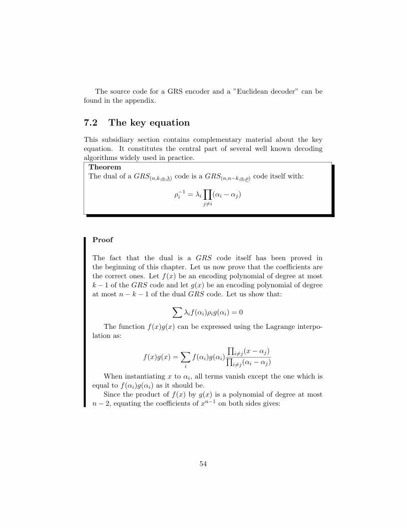
7.2 The key equation

This subsidiary section contains complementary material about the keyequation. It constitutes the central part of several well known decodingalgorithms widely used in practice.

TheoremThe dual of a GRS(n,k,α,λ) code is a GRS(n,n−k,α,ρ) code itself with:

ρ−1i = λi

∏j 6=i

(αi − αj)

Proof

The fact that the dual is a GRS code itself has been proved inthe beginning of this chapter. Let us now prove that the coefficients arethe correct ones. Let f(x) be an encoding polynomial of degree at mostk− 1 of the GRS code and let g(x) be an encoding polynomial of degreeat most n− k − 1 of the dual GRS code. Let us show that:∑

λif(αi)ρig(αi) = 0

The function f(x)g(x) can be expressed using the Lagrange interpo-lation as:

f(x)g(x) =∑i

f(αi)g(αi)

∏i 6=j(x− αj)∏i 6=j(αi − αj)

When instantiating x to αi, all terms vanish except the one which isequal to f(αi)g(αi) as it should be.

Since the product of f(x) by g(x) is a polynomial of degree at mostn− 2, equating the coefficients of xn−1 on both sides gives:

54

0 =∑i

f(αi)g(αi)1∏

i 6=j(αi − αj)

=∑i

λif(αi)1

λi∏i 6=j(αi − αj)

g(αi)

=∑i

(λif(αi))(ρig(αi))

Which completes the proof.

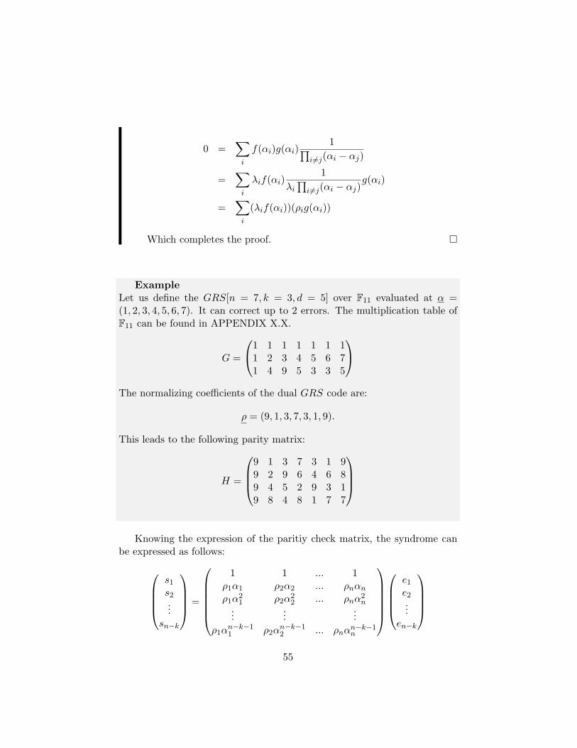
ExampleLet us define the GRS[n = 7, k = 3, d = 5] over F11 evaluated at α =(1, 2, 3, 4, 5, 6, 7). It can correct up to 2 errors. The multiplication table ofF11 can be found in APPENDIX X.X.

G =

1 1 1 1 1 1 11 2 3 4 5 6 71 4 9 5 3 3 5

The normalizing coefficients of the dual GRS code are:

ρ = (9, 1, 3, 7, 3, 1, 9).

This leads to the following parity matrix:

H =

9 1 3 7 3 1 99 2 9 6 4 6 89 4 5 2 9 3 19 8 4 8 1 7 7

Knowing the expression of the paritiy check matrix, the syndrome canbe expressed as follows:

s1

s2...

sn−k

=

1 1 ... 1

ρ1α1 ρ2α2 ... ρnαnρ1α

21 ρ2α

22 ... ρnα

2n

......

...ρ1α

n−k−11 ρ2α

n−k−12 ... ρnα

n−k−1n

e1

e2...

en−k

55

And, by isolating each component of the syndrome:

sj =∑i

eiρiαj−1i

Let us now take every syndrome component into account:

s(z) =n−k∑j=1

sjzj−1

=n−k∑j=1

∑i

eiρiαj−1i zj−1

=∑i

eiρi

n−k∑j=1

αj−1i zj−1

=∑i

eiρi

(1− (αiz)n−k

1− αiz

)Since terms with ei = 0 do not contribute to the latter sum, it is equivalentto consider this sum over the set of error locations I = i|ei 6= 0. With afew manipulations, the above equation becomes:∏

i∈I(1− αiz)s(z) =

∑i∈I

eiρi∏

j∈I\i

(1− αjz) (mod zn−k)

This expression can be expressed more elegantly as the key equation:

σ(z)s(z) = ω(z) (mod zn−k)

withσ(z) =

∏i∈I

(1− αiz)

andω(z) =

∑i∈I

eiρi∏

j∈I\i

(1− αjz) (mod zn−k)

The polynomial ω(z) is called the error locator polynomial because it tellsus at which coordinates the errors are:

I = i|σ(α−1i ) = 0

56

Once these error locations are known, the error evaluator polynomial ω(z)gives us the exact error at a given position:

∀i ∈ I : ei =ω(α−1

i )ρi∏j∈I\i(1− αjα

−1i )

Therefore, the decoding of a codeword necessitate to solve the key equationby finding σ(z) and ω(z). There exist several efficient techniques to do thisand we invite the interested reader to the extensive literature about thissubject, for example [1].

7.3 Conclusion

Reed-Solomon codes have many advantages. They provide excellent error-correcting abilities since they reach the Singleton bound. Moreover, k canbe chosen freely and therefore GRS codes can be used for nearly any rate.Lastly, they have efficient bounded distance decoding techniques decodingup to n−k

2 errors and polynomial running time in O(n2).One drawback they have is that they are based on large alphabets. If

they are mapped to smaller alphabets, their length and dimension increaseproportionally but their distance does not change. These mapped codeshowever remain excellent concerning error bursts since a block of successiveerrors affects only a few symbols in the bigger alphabet. Because error burstsis a common pattern, these codes are widely used in practice. Let us stressagain the fact that mapping a GRS code to a smaller alphabet is not wellsuited if the errors are completely random.

57

Part II

Soft decoding

58

Chapter 8

Introduction

8.1 What do we achieve here?

The algebraic algorithm we present here is a breakthrough in the field. Clas-sical algorithms either perform hard-decoding up to n−k

2 errors, or are run-ning in exponential time and were thus of very limited practical use due totheir complexity exploding behavior. This algorithm outperforms both byproviding soft-decoding in polynomial time. Moreover, it can handle hard-decoding also as a special case. For both, the gains are substantial. Forhard-decoding, it provides list-decoding beyond the classical n−k

2 bound forlow rates easily. For high rates this is also the case but the cost grows dras-tically in this latter case. However, its real strength lies in soft-decoding,taking advantage of the full information available. Using soft-decoding, theperformances improvement of the error correction ability is substantial whilerunning in polynomial time. Moreover, it has some other advantages. Forexample, the trades-off between decoding complexity and decoding perfor-mance can easily be fine tuned. Another side effect is that erasures arenaturally handled. Moreover, and not unimportant, the algorithm can beextended to BCH and algebraic-geometry codes. Lastly, as bonus if I maysay, the algorithm provides beautiful underlying mathematics.

8.2 History and results

In 1996, Sudan presented a new kind of algorithm for hard-decoding Reed-Solomon codes [5]. He placed the problem in a new light and transformedthe problem of decoding to a problem of polynomial fitting. This led to anew algorithm providing list-decoding beyond the error-correction radius of

59

n−k2 for low rate RS codes. This triggered a renewed and intense interest

in the research community. A few years later, Sudan and Guruswami ex-tended the algorithm and provided a better error-correction ability at anyrate [6]. However, increased error-correction ability comes hand-in-handwith increased computational cost. For high rate codes, these are significant.Then Koetter and Vardy generalized it one step further to take advantageof the soft-information from the channel [9]. This leads to the algebraic soft-decision Reed-Solomon decoding algorithm we present here. The algorithmhas two main parts consisting in interpolation and factorization of bivari-ate polynomials (over finite fields). For these two tasks, efficient solutionswere presented by [12] and [13]. Research is still active in this ”hot” area,various modifications and improvements were already published and furtheradvancements are to be expected.

8.3 General outline

The first chapter covers Sudan’s initial algorithm in full length. It offers anunderstanding of the global process, of the algorithm as a whole and will bevalid for the other algorithms too. Then, the extension of Guruswami-Sudanis implicitly presented in chapter two leading directly to a presentation ofthe core theorem of the algorithm: a condition on successful decoding. Thisis presented in a fashion naturally made to be extended to the soft-decodingadaptation from Koetter and Vardy in chapter three. This one consists of amapping of the soft-information from the channel to the multiplicity matrixintroduced later and a few comments on performances. While chapter onegave the overview and chapter two and three give reasons on why it worksand what conditions should be satisfied, the two next chapter are aboutpractical tasks. As for Sudan’s initial algorithm, two main steps remain:the interpolation and the factorization of a bivariate polynomial. Efficientways of performing these are seen in chapter four and five, respectively.Lastly, some recent improvements are briefly outlined, and a conclusion isgiven.

60

Chapter 9

The Sudan algorithm

In this chapter, we cover completely Sudan’s algorithm which pioneeredthe field. This algorithm was the first in its genre and the source of allthe subsequent algorithms like the algebraic soft decoding which is in factjust a layer upon it. Therefore, understanding the easier Sudan algorithmfirst helps greatly to understand the big picture and to grasp some of theunderlying concepts also valid for the other algorithms.

9.1 Introduction

In 1996, Madhu Sudan presented in [5] a new and innovative way of decod-ing Reed-Solomon and algebraic geometry codes. Before, every decodingscheme was based on the analysis of the syndrome. The new approach ofSudan is based on a geometrical interpretation of the problem. This didnot only opened new ways of considering the decoding problem of Reed-Solomon codes, but also provided a more powerful list-decoding. Before, allthe classical decoding algorithms decoded at a distance up to n−k

2 . We willsee that Sudan’s algorithm performs list-decoding beyond this bound for lowrate codes.

9.2 Decoding problem reformulation

As seen in chapter 7, codewords from a RS code are the evaluation of anencoding polynomial at given locations. Let some f(z) be the encodingpolynomial and let α = (α1, ..., αn) be the locations where it is evaluated.The codeword can be represented as a set of n points (αi, f(αi)) as we sawbefore.

61

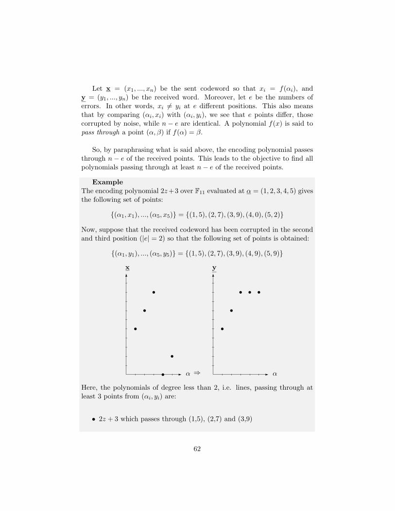
Let x = (x1, ..., xn) be the sent codeword so that xi = f(αi), andy = (y1, ..., yn) be the received word. Moreover, let e be the numbers oferrors. In other words, xi 6= yi at e different positions. This also meansthat by comparing (αi, xi) with (αi, yi), we see that e points differ, thosecorrupted by noise, while n − e are identical. A polynomial f(x) is said topass through a point (α, β) if f(α) = β.

So, by paraphrasing what is said above, the encoding polynomial passesthrough n− e of the received points. This leads to the objective to find allpolynomials passing through at least n− e of the received points.

ExampleThe encoding polynomial 2z+3 over F11 evaluated at α = (1, 2, 3, 4, 5) givesthe following set of points:

(α1, x1), ..., (α5, x5) = (1, 5), (2, 7), (3, 9), (4, 0), (5, 2)

Now, suppose that the received codeword has been corrupted in the secondand third position (|e| = 2) so that the following set of points is obtained:

(α1, y1), ..., (α5, y5) = (1, 5), (2, 7), (3, 9), (4, 9), (5, 9)

-

6

α

x

ss

s

ss

⇒ -

6

α

y

ss

s s s

Here, the polynomials of degree less than 2, i.e. lines, passing through atleast 3 points from (αi, yi) are:

• 2z + 3 which passes through (1,5), (2,7) and (3,9)

62

• 9 which passes through (3,9), (4,9) and (5,9)

In this case, both codewords would be at a distance 2 from y and aretwo equiprobable candidates for decoding.

What we get is a list of all polynomials corresponding to codewords at adistance at most e from the received codeword y. To our delight, the list isusually rather short. Before going further, it should be noted that we do notknow the value of e beforehand. Therefore, we will instead use a constant τdenoting the decoding radius, or in other words, the number of points thatcan differ.

As can be seen, the decoding problem has shifted from finding the near-est codeword to a polynomial fitting problem. This problem translation hastwo advantages. First, the polynomial fitting problem is more general sinceit can be generalized to other fields like the reals or complex while it canalso be used in a much larger panel of applications. Secondly, this abstrac-tion enables us to put codes by side. It is now a polynomial fitting problemand can be handled independently, without requesting any error-correctingcodes knowledge. However, the connection will be kept all the way since itis the aim of this work. To resume the whole, let us restate the problem torefresh our mind:

Input:

• n points: (αi, yi) for 1 ≤ i ≤ n

• the decoding radius τ

• the maximum degree k − 1 of the fitting polynomial

Output:

• a list L containing all polynomials f(z) of degree less than k passingthrough at least n− τ points.

As a reminder, this is equivalent to the decoding problem. Indeed, thepolynomials we will get will be the ones that encode codewords being at adistance less than or equal to τ from the received codeword.

The main question this triggers is: how to (efficiently) find those poly-nomials? Subsidiary questions are: for which values of τ does it work? And

63

lastly, how likely is it to obtain more than one fitting polynomial? All thesequestions will be answered in this order.

It is now time to introduce Sudan’s algorithm. Before we attack the coreof the algorithm and the key aspect, we will need to define some vocabulary.

9.3 Weighted degree

Definition 24 The (a, b) weighted degree of a monomial xiyj is defined as:

wdeg(a,b)xiyj = ai+ bj

Any polynomial is by definition just a finite weighted sum of monomials:Q(x, y) =

∑qijx

iyj . It is therefore natural to extend the definition ofweighted degree to polynomials in the following manner:

Definition 25 The (a,b) weighted degree of a polynomial Q(x, y) is thelargest weighted degree of its monomials.

Examplewdeg(1,7)x

2y3 = 2 + 3 ∗ 7 = 23wdeg(1,4)(x6 + x3y + xy2) = max(6, 7, 9) = 9

The notion of weighted degree can be extended to any number of vari-ables but two will suffice for our needs. The use of this can be illustratedin the following situation. Consider a bivariate polynomial Q(z, F ) and aunivariate polynomial f(z). If we replace F by f(z), we get:

Q(z, f(z)) =∑

qijzi(f(z))j

Therefore, if the maximum degree of f(z) is at most k−1 then the maximumdegree of Q(z, f(z)) is upper bounded by the (1, k − 1) weighted degree ofQ(z, F ).

9.4 Overview

The algorithm is based on a bivariate polynomial called Q(z, F ) 1 whose(1, k − 1) weighted degree is Ω. When F is replaced by a polynomial f(z)

1 It is often noted as Q(x, y) in the literature but we have preferred the Q(z, F ) notationin this text. The reason of this choice is to improve clarity and to avoid possible confusionbetween the variables x, y and the codewords x,y.

64

of degree less than k in Q(z, F ), we get a univariate polynomial Q(z, f(z))of degree less than or equal to Ω as seen previously.

Now, assume that we choose Q(z, F ) so that Q(αi, yi) = 0 for everyi. We say that Q(z, F ) is zero or vanishes at this point. An interestingviewpoint is the algebraic curve defined by Q(z, F ) = 0, this curve passesthrough every point (αi, yi).

If f(αi) = yi for some αi then Q(z, f(z)) is zero as well for this valueαi since Q(αi, f(αi)) = Q(αi, yi) = 0. Thus, every αi such that f(αi) = yiis also a root of the polynomial Q(z, f(z)). Therefore Q(z, f(z)) is eitherthe zero polynomial or has as many roots as the number of points that f(z)passes through.

In the case f(z) passes through more than Ω points, the polynomialQ(z, f(z)) should also have as many roots. Since a non-zero polynomialcannot have more roots than its degree, there is no other possibility thanbeing the zero polynomial. To summarize it, if f(z) passes through morethan Ω points, then Q(z, f(z)) = 0. Which in turn implies that f(z) is anF -root of Q(z, F )!

This condensed explanation will now be seen in more detail, step by stepand illustrated by a few examples for a better understanding.

9.5 Constraints for Q

The polynomial Q(z, F ) should have two properties, it should vanish at allpoints and have a weighted degree as small as possible. More formally,

Let Q(z, F ) = qijziF j , with qij ∈ Fq. We want to ensure that:

• Q(αi, yi) = 0 for every i.

• Ω = wdeg(1,k−1)Q(z, F )] is minimal.

The first condition regroups n constraints, one for each point, that wemust satisfy. To find an appropriate Q(z, F ) it is therefore sufficient to solvea system of n equation, one for each point, where the unknowns are thecoefficients qij of the polynomial and the ziF j terms are evaluated at eachpoint. A non-trivial solution exists provided that the number of unknowns isgreater than n. Or in other words, we need more than n distinct monomialsat hand.

65

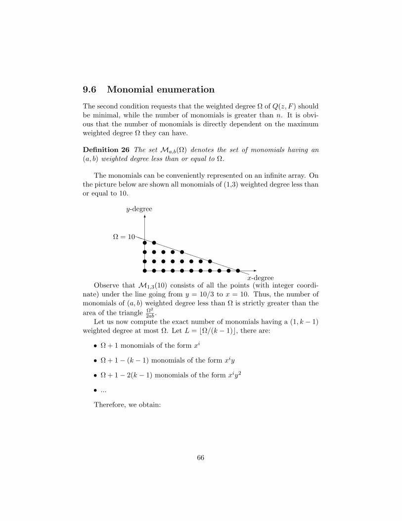
9.6 Monomial enumeration

The second condition requests that the weighted degree Ω of Q(z, F ) shouldbe minimal, while the number of monomials is greater than n. It is obvi-ous that the number of monomials is directly dependent on the maximumweighted degree Ω they can have.

Definition 26 The set Ma,b(Ω) denotes the set of monomials having an(a, b) weighted degree less than or equal to Ω.

The monomials can be conveniently represented on an infinite array. Onthe picture below are shown all monomials of (1,3) weighted degree less thanor equal to 10.

-

6

x-degree

y-degree

u u u u u u u u u u uu u u u u u u uu u u u uu uPPPPPPPPPPPPPPPPPPΩ = 10

Observe that M1,3(10) consists of all the points (with integer coordi-nate) under the line going from y = 10/3 to x = 10. Thus, the number ofmonomials of (a, b) weighted degree less than Ω is strictly greater than thearea of the triangle Ω2

2ab .Let us now compute the exact number of monomials having a (1, k − 1)

weighted degree at most Ω. Let L = bΩ/(k − 1)c, there are:

• Ω + 1 monomials of the form xi

• Ω + 1− (k − 1) monomials of the form xiy

• Ω + 1− 2(k − 1) monomials of the form xiy2

• ...

Therefore, we obtain:

66

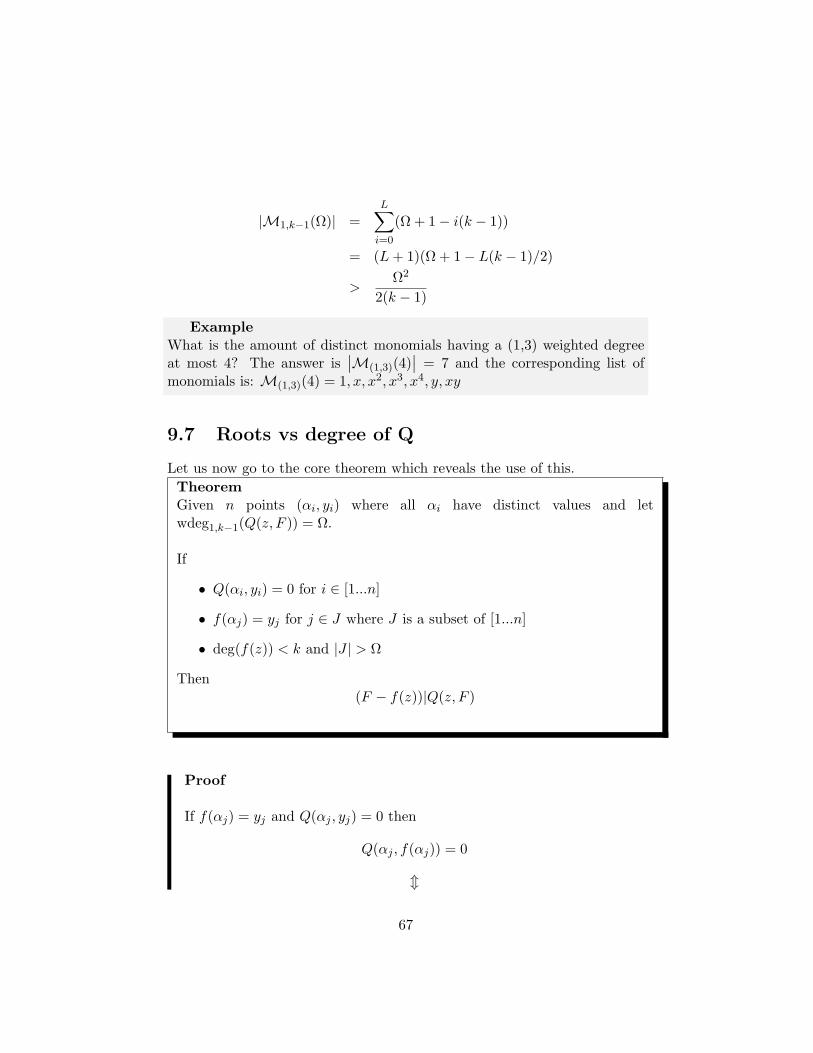
|M1,k−1(Ω)| =L∑i=0

(Ω + 1− i(k − 1))

= (L+ 1)(Ω + 1− L(k − 1)/2)

>Ω2

2(k − 1)

ExampleWhat is the amount of distinct monomials having a (1,3) weighted degreeat most 4? The answer is

∣∣M(1,3)(4)∣∣ = 7 and the corresponding list of

monomials is: M(1,3)(4) = 1, x, x2, x3, x4, y, xy

9.7 Roots vs degree of Q

Let us now go to the core theorem which reveals the use of this.TheoremGiven n points (αi, yi) where all αi have distinct values and letwdeg1,k−1(Q(z, F )) = Ω.

If

• Q(αi, yi) = 0 for i ∈ [1...n]

• f(αj) = yj for j ∈ J where J is a subset of [1...n]

• deg(f(z)) < k and |J | > Ω

Then(F − f(z))|Q(z, F )

Proof

If f(αj) = yj and Q(αj , yj) = 0 then

Q(αj , f(αj)) = 0

m

67

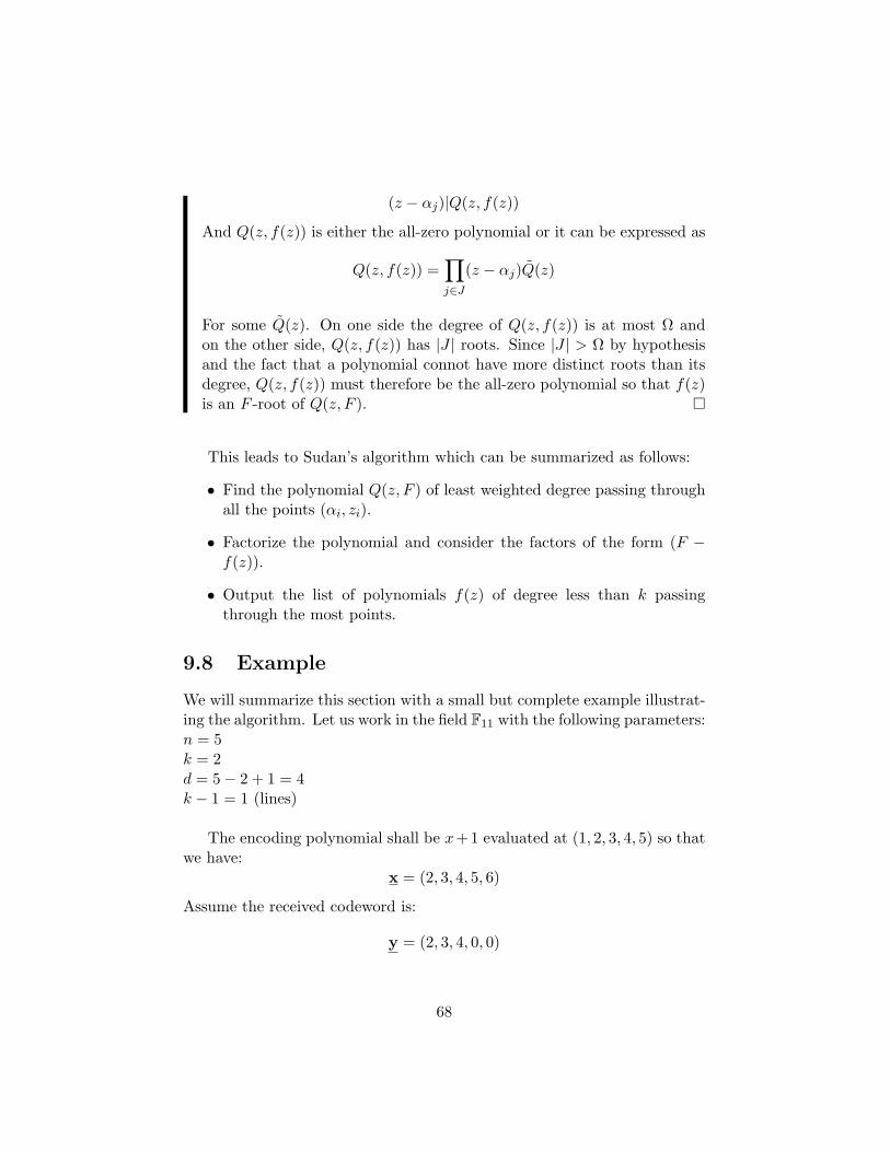
(z − αj)|Q(z, f(z))

And Q(z, f(z)) is either the all-zero polynomial or it can be expressed as

Q(z, f(z)) =∏j∈J

(z − αj)Q(z)

For some Q(z). On one side the degree of Q(z, f(z)) is at most Ω andon the other side, Q(z, f(z)) has |J | roots. Since |J | > Ω by hypothesisand the fact that a polynomial connot have more distinct roots than itsdegree, Q(z, f(z)) must therefore be the all-zero polynomial so that f(z)is an F -root of Q(z, F ).

This leads to Sudan’s algorithm which can be summarized as follows:

• Find the polynomial Q(z, F ) of least weighted degree passing throughall the points (αi, zi).

• Factorize the polynomial and consider the factors of the form (F −f(z)).

• Output the list of polynomials f(z) of degree less than k passingthrough the most points.

9.8 Example

We will summarize this section with a small but complete example illustrat-ing the algorithm. Let us work in the field F11 with the following parameters:n = 5k = 2d = 5− 2 + 1 = 4k − 1 = 1 (lines)

The encoding polynomial shall be x+ 1 evaluated at (1, 2, 3, 4, 5) so thatwe have:

x = (2, 3, 4, 5, 6)

Assume the received codeword is:

y = (2, 3, 4, 0, 0)

68

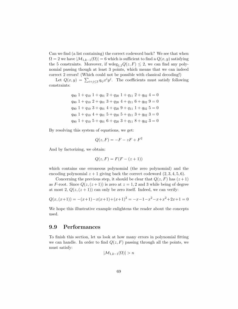
Can we find (a list containing) the correct codeword back? We see that whenΩ = 2 we have |M1,k−1(Ω)| = 6 which is sufficient to find a Q(x, y) satisfyingthe 5 constraints. Moreover, if wdeg1,1Q(z, F ) ≤ 2, we can find any poly-nomial passing though at least 3 points, which means that we can indeedcorrect 2 errors! (Which could not be possible with classical decoding!)

Let Q(x, y) =∑

i+j≤3 qijxiyj . The coefficients must satisfy following

constraints:

q00 1 + q10 1 + q01 2 + q20 1 + q11 2 + q02 4 = 0q00 1 + q10 2 + q01 3 + q20 4 + q11 6 + q02 9 = 0q00 1 + q10 3 + q01 4 + q20 9 + q11 1 + q02 5 = 0q00 1 + q10 4 + q01 5 + q20 5 + q11 3 + q02 3 = 0q00 1 + q10 5 + q01 6 + q20 3 + q11 8 + q02 3 = 0

By resolving this system of equations, we get:

Q(z, F ) = −F − zF + F 2

And by factorizing, we obtain:

Q(z, F ) = F (F − (z + 1))

which contains one erroneous polynomial (the zero polynomial) and theencoding polynomial z + 1 giving back the correct codeword (2, 3, 4, 5, 6).

Concerning the previous step, it should be clear that Q(z, F ) has (z+ 1)as F -root. Since Q(z, (z+ 1)) is zero at z = 1, 2 and 3 while being of degreeat most 2, Q(z, (z + 1)) can only be zero itself. Indeed, we can verify:

Q(x, (x+1)) = −(x+1)−x(x+1)+(x+1)2 = −x−1−x2−x+x2+2x+1 = 0

We hope this illustrative example enlightens the reader about the conceptsused.

9.9 Performances

To finish this section, let us look at how many errors in polynomial fittingwe can handle. In order to find Q(z, F ) passing through all the points, wemust satisfy:

|M1,k−1(Ω)| > n

69

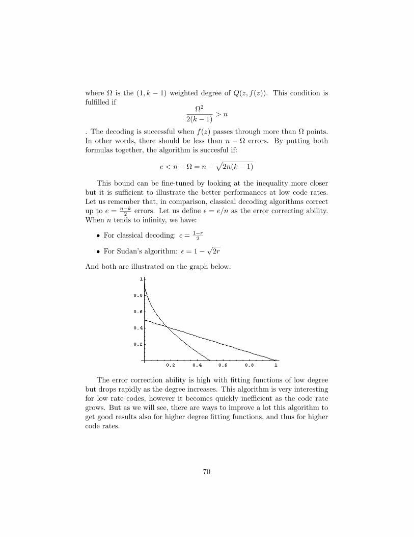
where Ω is the (1, k − 1) weighted degree of Q(z, f(z)). This condition isfulfilled if

Ω2

2(k − 1)> n

. The decoding is successful when f(z) passes through more than Ω points.In other words, there should be less than n − Ω errors. By putting bothformulas together, the algorithm is succesful if:

e < n− Ω = n−√

2n(k − 1)

This bound can be fine-tuned by looking at the inequality more closerbut it is sufficient to illustrate the better performances at low code rates.Let us remember that, in comparison, classical decoding algorithms correctup to e = n−k

2 errors. Let us define ε = e/n as the error correcting ability.When n tends to infinity, we have:

• For classical decoding: ε = 1−r2

• For Sudan’s algorithm: ε = 1−√

2r

And both are illustrated on the graph below.

The error correction ability is high with fitting functions of low degreebut drops rapidly as the degree increases. This algorithm is very interestingfor low rate codes, however it becomes quickly inefficient as the code rategrows. But as we will see, there are ways to improve a lot this algorithm toget good results also for higher degree fitting functions, and thus for highercode rates.

70

Chapter 10

Zeros, roots and constraints

This chapter is devoted to understanding the relationship between higherorder zeros, the roots of Q(z, f(z)) and the constraints on the polynomialQ(z, F ) to satisfy these zeros. Using the algebraic curve comparison, itmeans that the curve passes through given points several times. In Sudan’salgorithm, Q(z, F ) is determined so that it is zero at each received point.The idea remains the same but it is generalized to each point with zeros ofany multiplicity. The consequences of this will be the core theorem of thealgorithm seen in the next chapter.

10.1 Zeros of higher multiplicity

For a univariate polynomial f(x) = f0 + f1x + f2x2 + f3x

3 + f4x4 + ...,

we say that f(x) has a zero of multiplicity (or order) m at the origin iff0 = f1 = ... = fm−1 = 0 so that it can be expressed as f(x) =

∑i≥m fix

i.Or equivalently we can say that xm|f(x). All these conditions are strictlyequivalent. As a side note, a null multiplicity is no zero at all.

To know the multiplicity of a zero at a given point α, we just have totranslate the polynomial so that its new origin is at α. This corresponds tothe translated polynomial f(x+α). Therefore, the zero multiplicity of f(x)at α is simply the zero multiplicity of f(x+ α) at the origin.

We can define the multiplicity of zeros for Q(z, F ) exactly the same way.

Definition 27 A polynomial Q(z, F ) has a zero of multiplicity or order mat (α, β) if Q(z + α, F + β) =

∑i+j≥m qijz

iF j.

Q(z + α, F + β) is simply the polynomial Q(z, F ) where the origin hasbeen translated to the point (α, β). Having a multiplicity of m just means

71

that this translated polynomial has no monomials of degree less than m.

Recall that in the Sudan algorithm, we proved that if f(α) = β andQ(α, β) = 0 then (z − α)|Q(z, f(z)). This result will now be extended tozeros of higher multiplicities in the following theorem.

TheoremDIVISORS THEOREMIf Q(z, F ) has a zero of order m at (α, β) and f(α) = β then

(z − α)m|Q(z, f(z))

Proof

By translation of z to z + α, proving that (z − α)m|Q(z, f(z)) isequivalent to proving that zm|Q(z + α, f(z + α)).

Let us now consider the polynomial f(z + α)− β. Since it is zero atthe origin (for z = 0), we can rewrite it to become f(z + α)− β = zf(z)for some f(z).

By replacing f(z + α) in the translated equation, we get Q(z +α, zf(x) +β) and since Q(z, F ) has a zero of order m at (α, β) we get thefinal expression:

Q(z + α, zf(z) + β) =∑

i+j≥mqijz

izj f(z)k

which is divisible by zm as we wanted to show.

ExampleLet f(z) = z2 − 4 and Q(z, F ) = (F − z − 2)2.

When (α, β) = (3, 5), it can be shown that f(α) = β and Q(z, F ) has azero of multiplicity 2 at this point. Let us verify this. For f(α) we have:

f(3) = 9− 4 = 5.

And for Q(z + α, F + β) we have:

Q(z + 3, F + 5) = ((F + 5)− (z + 3)− 2)2 = (F − z)2

72

which has indeed a zero of multiplicity two.Lastly, the theorem tells us that (z − 3)2|Q(z, f(z)) in this case and we

can verify:

Q(z, f(z)) = (z2 − z − 6)2 = (z − 3)2(z + 2)2.

And the desired result is obtained.

This can now be extended to any number of points. If f(z) passesthrough n such points (αi, βi) and Q(z, F ) has zeros of multiplicity mi atthese, then we have: ∏

i

(z − αi)mi |Q(z, f(z))

This is exactly the same reasoning as for Sudan’s algorithm.

10.2 Expressing the constraints

Let us now rename the parameters of Q(z, F ) to become Q(x, y). This isjust a renaming for convenience, x has nothing to do with a codeword andjust stands for z. And as well about y which just stands for F . The subjectof this section is to determine the constraints that Q(x, y) must satisfy inorder to have zeros of given multiplicities at given points. Or better said, ifwe express Q(x, y) as:

Q(x, y) =∑

qijxiyj

The question becomes: how can the coefficients qij be chosen so that Q(x, y)has indeed zeros of given multiplicities at the given points? More precisely,for some points (α, β), the polynomial Q(x, y) must have a zero of multi-plicity m. This means that

Q(x+ α, y + β) =∑

i+j≥mq(α,β),ijx

iyj

where q(α,β),∗ are the coefficients of the polynomial translated to the point(α, β).

Since the translation is a linear transformation, the translated coefficientsq(α,β),ij can be expressed as a linear combination of the original ones. To

73

see this, let us decompose the translated polynomial:

Q(x+ α, y + β) =∑i,j

qij(x+ α)i(y + β)j

=∑i,j

qij

[i∑

u=0

(iu

)xuαi−u

][j∑

v=0

(jv

)yvβj−v

]

Now we can establish a relationship between the coefficients q∗ of the initialpolynomial and the coefficients q(α,β),∗ of the translated one. By isolatingterms of given degree xuyv from Q(x+ α, y + β), we obtain:

q(α,β),uv = coef(xuyv) =∑

i≥u,j≥vqij

(iu

)(jv

)αi−uβj−v

In a field of characteristic 0, this awkward expression is equivalent to avery convenient one, namely the Hasse derivative.

Definition 28 The (u, v)th Hasse (mixed partial) derivative of Q(x, y) eval-uated at (α, β) is:

DHu,v,(α,β) Q(x, y) =(

1u!v!

du

dxudv

dyvQ(x, y)

)∣∣∣∣(α,β)

Indeed, this definition is equivalent to the previous expression (...providedthe field is of characteristic 0). The sharp-eyed reader may have noticed thatin other fields, the Hasse derivative would in some cases reduce to 0

0 if wetreat it in a rigorous way. For example, the pth derivative of xn in Fq, whereq is a power of p, would reduce to 0

0 since in this field p ≡ 0. Therefore, thetwo expressions are quite similar but are not strictly equivalent because ofthe field characteristic. From now on, we shall use the notation Du,v,(α,β) toexpress the coefficients q(α,β),uv to remind the extreme similarity with theHasse derivative.

q(α,β),uv = coef(xuyv) = Du,v,(α,β)Q(x, y)

ExampleLet Q(x, y) = x3 + y2 + xy ∈ F11[x, y] and the point (2, 5). What are thecoefficients q(2,5),ij of Q(x+ 2, y + 5)?

We have:

74

D0,0,(2,5) Q(x, y) = (x3 + y2 + xy)∣∣(2,5)

= 43 = −1(mod11)

D1,0,(2,5) Q(x, y) = (3x2 + y)∣∣(2,5)

= 17 = 6(mod11)

D2,0,(2,5) Q(x, y) = (3x)|(2,5) = 6(mod11)D3,0,(2,5) Q(x, y) = 1D0,1,(2,5) Q(x, y) = (2y + x)|(2,5) = 12 = 1(mod11)D1,1,(2,5) Q(x, y) = 1D0,2,(2,5) Q(x, y) = 1

Thus, Q(x+ 2, y + 5) can be expressed as:

Q(x+ 2, y + 5) = y2 + xy + y + x3 + 6x2 + 6x− 1

In order to have a zero of multiplicity m at (α, β), we must have all thecoefficients of the translated polynomial qi,uv = 0 whenever u+v ≤ m. Thisis equivalent to satisfying the set of constraints:

D = Du,v,(α,β) Q(x, y) = 0|u+ v ≤ m

And this set contains m(m+1)2 linear constraints since this is the number of

couples u, v satisfying u+ v ≤ m.This can be generalized to any number of points with zeros of any multi-

plicities easily. Moreover, each constraint can be expressed as a linear com-bination of the coefficients from the initial polynomial Q(x, y). A system oflinear equations is obtained where each equation expresses a constraint.

ExampleLet Q(x, y) = q00 + q10x+ q20x

2 + q01y + q11xy. Is it possible to find valuesfor the different qij so that Q(x, y) has a zero of order 2 at p = (2, 3)?

The answer is yes! Indeed Q(x, y) has a zero of order 2 at p if it satisfiesthis set of constraints:

D = D0,0,p, D1,0,p, D0,1,pSo that the following system of equations is obtained:

D0,0,pQ = q00 + 2q10 + 4q20 + 3q01 + 6q11 = 0D1,0,pQ = q10 + 4q20 + 3q11 = 0D0,1,pQ = q01 + 2q11 = 0

75

By solving it, we obtain that Q(x, y) can be any linear combination of:

4− 4x+ x2 and 6− 3x− 2y + xy

When we take a closer look at both of these components, we see that theyare equivalent to:

(x− 2)2 and (x− 2)(y − 3)

And it is easily seen that both of these components have second order zerosat (2, 3).

To conclude, let us say that Q(x, y) can be found in polynomial timesince it is sufficient to solve a system of linear equations expressing therequired constraints. Since a zero of multiplicity mi at a point pi can beexpressed as mi(mi+1)

2 linear constraints on the coefficients of Q(x, y), weobtain a system of linear equations with

∑imi(mi+1)

2 constraints.Finding a nonzero polynomial satisfying these constraints can be done by

solving a system of linear equations provided that there are more coefficientsthan constraints. Therefore, the weighted degree ofQ(x, y) must be just highenough to have more coefficients than this value.

76

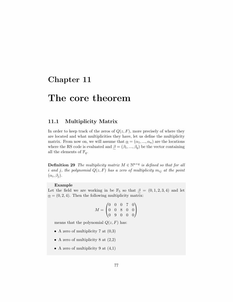
Chapter 11

The core theorem

11.1 Multiplicity Matrix

In order to keep track of the zeros of Q(z, F ), more precisely of where theyare located and what multiplicities they have, let us define the multiplicitymatrix. From now on, we will assume that α = (α1, ..., αn) are the locationswhere the RS code is evaluated and β = (β1, ..., βq) be the vector containingall the elements of Fq.

Definition 29 The multiplicity matrix M ∈ Nn×q is defined so that for alli and j, the polynomial Q(z, F ) has a zero of multiplicity mij at the point(αi, βj).

ExampleLet the field we are working in be F5 so that β = (0, 1, 2, 3, 4) and letα = (0, 2, 4). Then the following multiplicity matrix:

M =

0 0 0 7 00 0 8 0 00 9 0 0 0

means that the polynomial Q(z, F ) has:

• A zero of multiplicity 7 at (0,3)

• A zero of multiplicity 8 at (2,2)

• A zero of multiplicity 9 at (4,1)

77

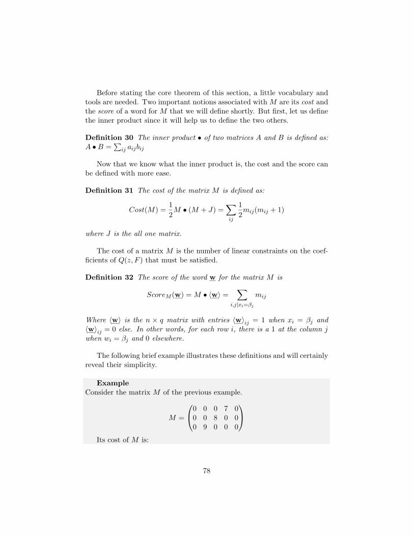
Before stating the core theorem of this section, a little vocabulary andtools are needed. Two important notions associated with M are its cost andthe score of a word for M that we will define shortly. But first, let us definethe inner product since it will help us to define the two others.

Definition 30 The inner product • of two matrices A and B is defined as:A •B =

∑ij aijbij

Now that we know what the inner product is, the cost and the score canbe defined with more ease.

Definition 31 The cost of the matrix M is defined as:

Cost(M) =12M • (M + J) =

∑ij

12mij(mij + 1)

where J is the all one matrix.

The cost of a matrix M is the number of linear constraints on the coef-ficients of Q(z, F ) that must be satisfied.

Definition 32 The score of the word w for the matrix M is

ScoreM (w) = M • 〈w〉 =∑

i,j|xi=βj

mij

Where 〈w〉 is the n × q matrix with entries 〈w〉ij = 1 when xi = βj and〈w〉ij = 0 else. In other words, for each row i, there is a 1 at the column jwhen wi = βj and 0 elsewhere.

The following brief example illustrates these definitions and will certainlyreveal their simplicity.

ExampleConsider the matrix M of the previous example.

M =

0 0 0 7 00 0 8 0 00 9 0 0 0

Its cost of M is:

78

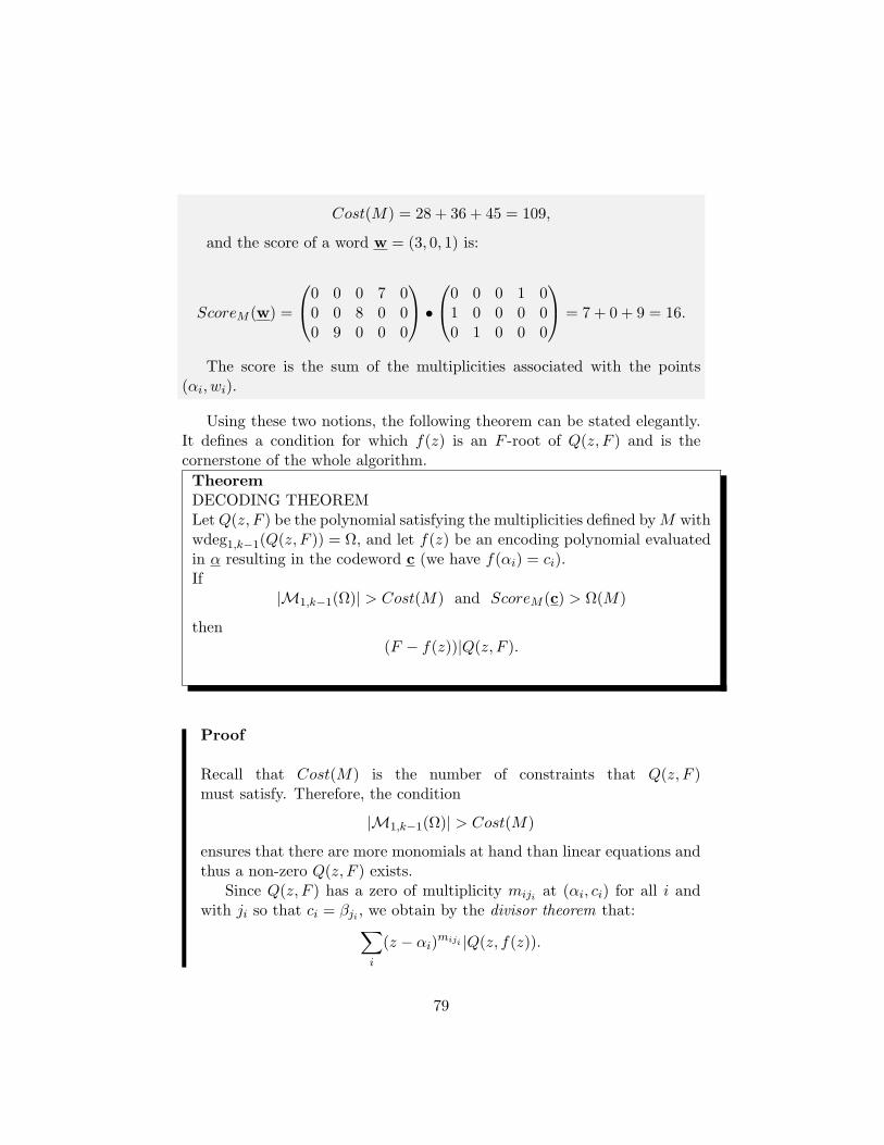
Cost(M) = 28 + 36 + 45 = 109,

and the score of a word w = (3, 0, 1) is:

ScoreM (w) =

0 0 0 7 00 0 8 0 00 9 0 0 0

•0 0 0 1 0

1 0 0 0 00 1 0 0 0

= 7 + 0 + 9 = 16.

The score is the sum of the multiplicities associated with the points(αi, wi).

Using these two notions, the following theorem can be stated elegantly.It defines a condition for which f(z) is an F -root of Q(z, F ) and is thecornerstone of the whole algorithm.

TheoremDECODING THEOREMLetQ(z, F ) be the polynomial satisfying the multiplicities defined byM withwdeg1,k−1(Q(z, F )) = Ω, and let f(z) be an encoding polynomial evaluatedin α resulting in the codeword c (we have f(αi) = ci).If

|M1,k−1(Ω)| > Cost(M) and ScoreM (c) > Ω(M)

then(F − f(z))|Q(z, F ).

Proof

Recall that Cost(M) is the number of constraints that Q(z, F )must satisfy. Therefore, the condition

|M1,k−1(Ω)| > Cost(M)

ensures that there are more monomials at hand than linear equations andthus a non-zero Q(z, F ) exists.

Since Q(z, F ) has a zero of multiplicity miji at (αi, ci) for all i andwith ji so that ci = βji , we obtain by the divisor theorem that:∑

i

(z − αi)miji |Q(z, f(z)).

79

Thus, the polynomial Q(z, f(z)) is either the all-zero polynomial or has(at least)

∑imiji = ScoreM (c) roots.

Recall that the degree of Q(z, f(z)) is bounded from above by theweighted degree of Q(z, F ), equal to Ω. Thus, when

ScoreM (c) > Ω(M)

then the polynomial Q(z, f(z)) would have more roots than its degree andit must therefore be the all-zero polynomial. In other words, we have:

(F − f(z))|Q(z, F )

which concludes the proof.

Let us stress that understanding the previous theorem and its proof iscrucial. That f(z) is an F -root of Q(z, F ) means that we can ”extract it”by factorizing Q(z, F ). This reduces to a very simple but strong statement:if

ScoreM (x) > Ω(M)

then the decoding is successful. The algorithm naturally flows from thetheorem and is presented in the upcoming section. For the moment, we canalready see that increasing the multiplicities in M increases the potentialscore as well as the cost of the matrix. Thus, it is important to choose thevalues in a suitable manner. We will see that with higher values we canobtain finer decoding but since the cost of M is the number of constraintsto satisfy, it is directly linked to the algorithm complexity. This provides atrade-off between correction ability and computational complexity.

11.2 Algorithm and example

The algorithm steps can be illustrated as follows:

80

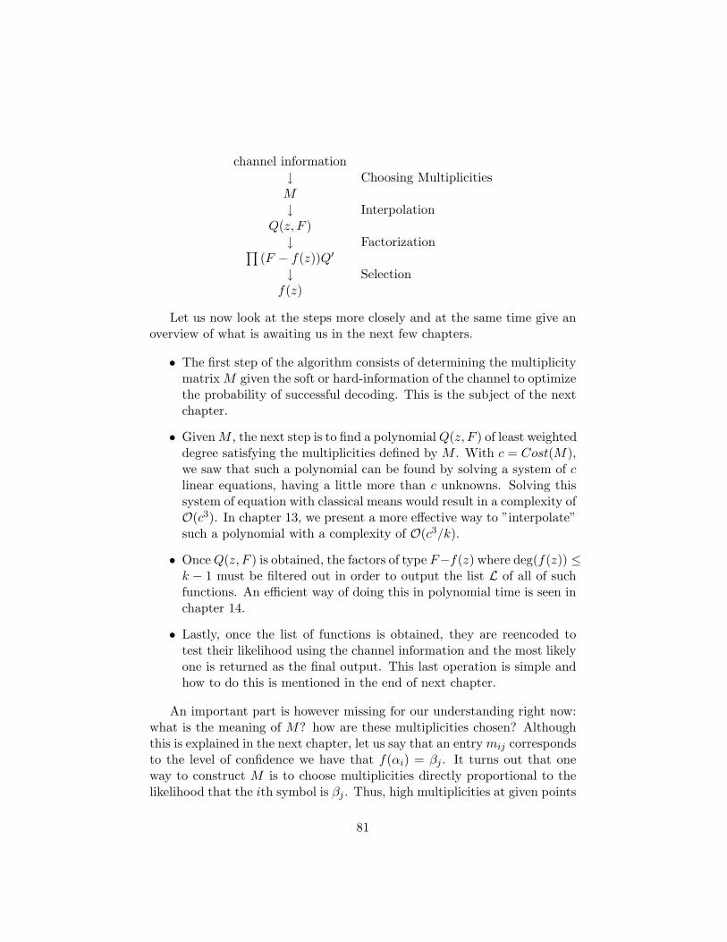
channel information↓ Choosing MultiplicitiesM↓ Interpolation

Q(z, F )↓ Factorization∏

(F − f(z))Q′

↓ Selectionf(z)

Let us now look at the steps more closely and at the same time give anoverview of what is awaiting us in the next few chapters.

• The first step of the algorithm consists of determining the multiplicitymatrix M given the soft or hard-information of the channel to optimizethe probability of successful decoding. This is the subject of the nextchapter.

• GivenM , the next step is to find a polynomialQ(z, F ) of least weighteddegree satisfying the multiplicities defined by M . With c = Cost(M),we saw that such a polynomial can be found by solving a system of clinear equations, having a little more than c unknowns. Solving thissystem of equation with classical means would result in a complexity ofO(c3). In chapter 13, we present a more effective way to ”interpolate”such a polynomial with a complexity of O(c3/k).

• OnceQ(z, F ) is obtained, the factors of type F−f(z) where deg(f(z)) ≤k − 1 must be filtered out in order to output the list L of all of suchfunctions. An efficient way of doing this in polynomial time is seen inchapter 14.

• Lastly, once the list of functions is obtained, they are reencoded totest their likelihood using the channel information and the most likelyone is returned as the final output. This last operation is simple andhow to do this is mentioned in the end of next chapter.

An important part is however missing for our understanding right now:what is the meaning of M? how are these multiplicities chosen? Althoughthis is explained in the next chapter, let us say that an entry mij correspondsto the level of confidence we have that f(αi) = βj . It turns out that oneway to construct M is to choose multiplicities directly proportional to thelikelihood that the ith symbol is βj . Thus, high multiplicities at given points

81

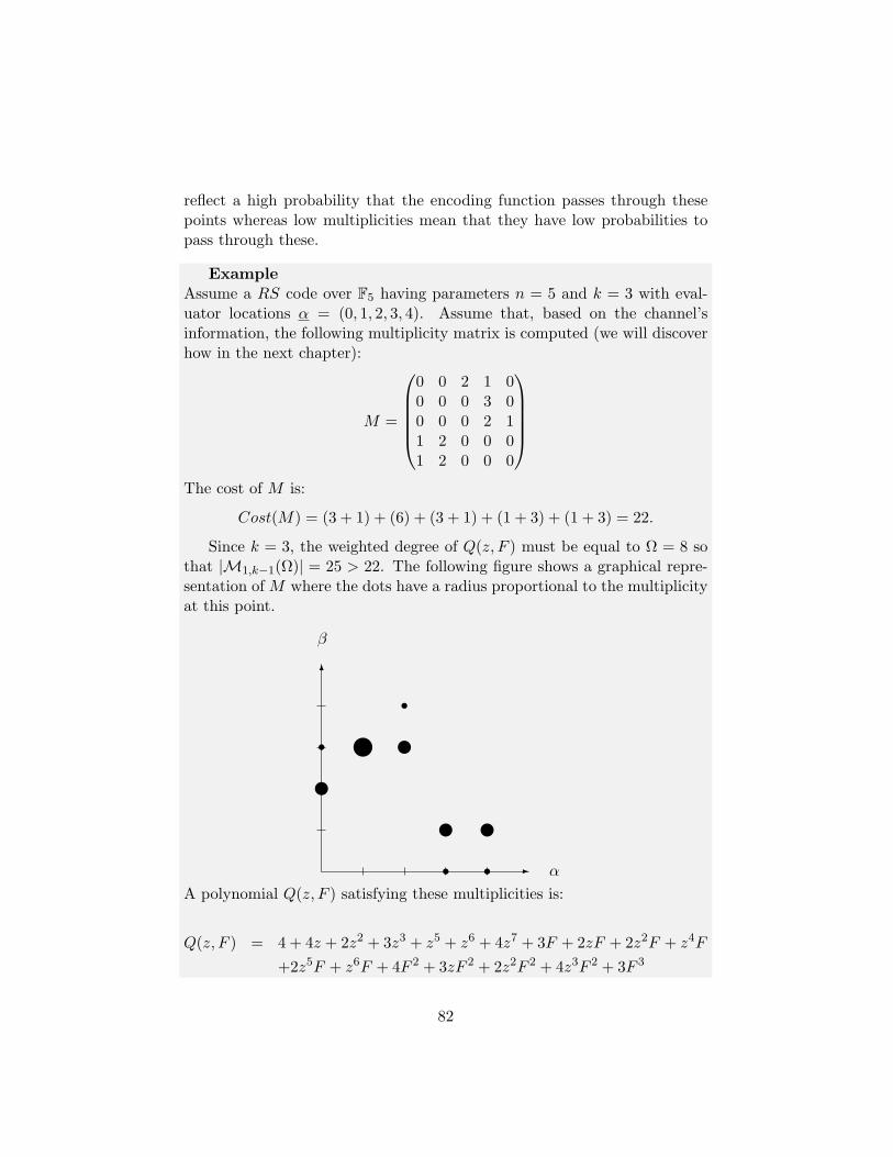
reflect a high probability that the encoding function passes through thesepoints whereas low multiplicities mean that they have low probabilities topass through these.

ExampleAssume a RS code over F5 having parameters n = 5 and k = 3 with eval-uator locations α = (0, 1, 2, 3, 4). Assume that, based on the channel’sinformation, the following multiplicity matrix is computed (we will discoverhow in the next chapter):

M =

0 0 2 1 00 0 0 3 00 0 0 2 11 2 0 0 01 2 0 0 0

The cost of M is:

Cost(M) = (3 + 1) + (6) + (3 + 1) + (1 + 3) + (1 + 3) = 22.

Since k = 3, the weighted degree of Q(z, F ) must be equal to Ω = 8 sothat |M1,k−1(Ω)| = 25 > 22. The following figure shows a graphical repre-sentation of M where the dots have a radius proportional to the multiplicityat this point.

-

6

α

β

xs | x

s

sx

sx

A polynomial Q(z, F ) satisfying these multiplicities is:

Q(z, F ) = 4 + 4z + 2z2 + 3z3 + z5 + z6 + 4z7 + 3F + 2zF + 2z2F + z4F

+2z5F + z6F + 4F 2 + 3zF 2 + 2z2F 2 + 4z3F 2 + 3F 3

82

By factorizing it, we obtain:

Q(z, F ) = [F − (2 + z)][F − (2 + 2z)][F − (3 + z + z2)]

Thus, three potential encoding functions are considered:

• z + 2

• 2z + 2

• 3 + z + z2

When computing the points they pass through and summing the multi-plicities at these points, we conclude that a single function has a high enoughscore, namely:

f(z) = z + 2.

The function passes through the points

(0, 2), (1, 3), (2, 4), (3, 0), (4, 1)

And its score x is:

ScoreM (x) = 2 + 3 + 1 + 1 + 2 = 9 > Ω = 8

Computing the score can be done quickly by looking at the graph above andlooking at the multiplicities of the points directly. In the end, the algorithmoutputs f(z) = z + 2 which is the best candidate for decoding.

83

Chapter 12

Multiplicity assignment

In the previous chapter, we saw that the output list of the algorithm containsthe sent codeword x ∈ C under the following condition:

ScoreM (x) > Ω(M),

where Ω(M) is the smallest integer such that |M1,k−1(Ω)| > Cost(M).Knowing this, the remaining question is: how to choose the matrix M?

This chapter shows how to find ”good” matrices M in the sense that theymaximize the probability of correct decoding, or better said, an approxima-tion thereof.

12.1 The reliability matrix

Let us start where everything starts: the channel. In our case, the inputconsists of symbols taken from a finite set, namely the elements of the fieldFq. We will denote the input as the discrete variable X which takes valuesin Fq.

Under the assumption that the channel is memoryless, it can be char-acterized by transition functions p(Y = y|X = βj) for every βj ∈ Fq. Theydefine the probability of receiving y when having sent βj .

Given these probabilities, it is easy to compute the reverse conditionalprobabilities using Bayes’ rule:

p(X = βj |Y = y) =p(y|X = βj)p(X = βj)∑l p(y|X = βl)p(X = βl)

Moreover, under the assumption that X is uniformly distributed over Fq,

84

the above formula can be simplified into:

p(X = βj |Y = y) =p(y|X = βj)∑l p(y|X = βl)

If we perform this computation for every received symbol yi, we obtain thereliability matrix.

Definition 33 The reliability matrix Π is an n × q matrix with entriesdefined as: πi,j = p(Xi = βj |Yi = yi).

To summarize it, each entry of Π is the probability that the ith symbolfrom the sent codeword is βj . We saw in the previous chapter that a code-word from an RS code can be represented as a set of n points (αi, xi = f(αi)).Placed in this light, the entries correspond to the confidence we have thatf(αi) = βj (based on the yi value received).

The sent and received codewords can be represented, respectively, bya vector of random variables X = (X1, ...,Xn) and Y = (Y1, ...,Yn). Notehowever that the a posteriori probability p(X = x|Y = y) are not equal to∏i p(X = xi|Y = yi) since the Xi are not independent. The equality would

apply if the vectors x would a priori be taken from Fnq . However, this isnot the case since they are taken from C(n,k) ⊂ Fnq . Moreover, it should bepointed out that finding p(X = x|Y = y) would be equivalent to maximumlikelihood decoding which is NP-complete.

12.2 Setting the problem

The sent codeword x is unknown to the decoder. The only information thedecoder has at hand is some stochastic information about the likelihood ofeach sent symbol. Therefore, from the decoder’s perspective, the sent code-word can be seen as a random variable X = (X1, ...,Xn). The probabilitythat a codeword w ∈ Fnq was sent can be stated as follows:

p(X = w|y) =

0 if w /∈ Cγ−1

∏p(Xi = wi|yi) if w ∈ C

where γ =∑

c∈C∏i p(Xi = ci|yi).

Given this distribution, the optimal multiplicity matrix Mopt is the onewhich maximizes the probability of decoding:

Mopt = argmaxMoptp(ScoreM (X ) > Ω(M))

85

Unfortunately, this optimization problem is inherently difficult because oftwo reasons:

• the matrix M affecting both sides of the inequality,

• the conditional probabilistic model for p(X = x).

Moreover, Koetter and Vardy showed that this optimization problem is nottractable and that finding the optimal Mopt reduces to an NP-hard prob-lem [9]. Therefore, a simplified model is used, tackling both of the abovedifficulties while remaining a good approximation.

Let Mc be the (finite) set of matrices whose cost is c. To deal with thefirst issue, the solution is to find M ∈ Mc maximizing the expected scoreamong matrices of equal cost c, that is

M = argmaxM∈McE[ScoreM (X )].

The justification is twofold. First, it sounds intuitively reasonable and makessense. Secondly, Koetter and Vardy computed bounds on the error proba-bility based on this approximation showing it is asymptotically ”good” [9].

Based on this reformulated problem, we are now concerned with how tocompute the expected score E[ScoreM (X )] of a matrix M . To do this, thefollowing approximation is needed, concerning the probability that x wassent:

p(X = x|y) =∏

p(Xi = xi|yi).

This would be the a posteriori distribution of X given y if the codewordswere a priori uniformly taken in the entire space Fnq . Therefore, the decoderdoes not use all the available information and this results in a sub-optimalproblem. However, it enables one to solve the (approximate) optimizationmodel because the expectation of the score can now be computed:

E[ScoreM (X )] =def∑

x∈Fnq

M • xp(X = x|y)

= M •∑

x∈Fnq

xp(X = x|y)

= M •Π.

Indeed, Π is the component-wise addition of 〈x〉 p(x). To conclude thissection, we thus look for M such that

M = argmaxM∈McM •Π

The two upcoming sections present two multiplicity assignment algo-rithms, shortly MAAs, solving exactly this approximated problem.

86

12.3 Greedy MAA

One way to findM ∈Mc which maximizesM•Π is to construct it iteratively.Starting with M0 as the all-zero matrix, the algorithm greedily incrementsone of the entries of M at each iteration. Incrementing an entry by one hastwo consequences:

• the cost is increased by mij + 1, this is the number of additional con-straints to satisfy;

• the expected score is increased by πij .

Therefore, the best choice is to increment the entry having the best tradeoff between gain and cost, that is, the greatest ratio πij

mij+1 .

TheoremInput:

• the reliability matrix Π

• an integer s, indicating the number of interpolation points

Output:the multiplicity matrix M = argmaxMM •Π among matrices of same cost.

Proof

Let us prove that the output of the algorithm is indeed the matrixM = argmaxMM • Π among the matrices of same cost. To facilitatethe understanding, a geometric interpretation is used. Let us associateto each position in M an infinite sequence of rectangles Rij,1, Rij,2, ...having their length and height defined as follows:

• length(Rij,l) = l

• height(Rij,l) = πij/l

Notice that the area of a rectangle Rij,l is πij . Now, let the set of rectan-gles associated to a multiplicity matrix M be

R = Rij,l|1 ≤ i ≤ n, 1 ≤ j ≤ q, 1 ≤ l ≤ mij

87

This set contains s rectangles, the number of interpolation points countedwith their multiplicities. Increasing the entry mij is by analogy addingthe rectangle Rij,mij+1, where its length is the number of constraintsadded and its area is the increase of the expected score. By putting allthese rectangles side by side, the cost of M can conveniently be expressedas the total length of the rectangles:

Cost(M) =12

∑ij

mij(mij + 1) =∑ij

mij∑l=1

l =∑R∈R

length(R).

And the expected score of M is the total surface of all rectangles:

M •Π =∑ij

mijπij =∑ij

mij∑l=1

πij =∑R∈R

area(R).

In this context, maximizing M for a given cost is equivalent to maximizingthe total area given its total length. It is obvious to see that this is doneby taking the set of the tallest rectangles and this is exactly what thealgorithm does. At each iteration, it picks the tallest rectangle.

Notice that no comment was made about the number of iterations s =∑mij which is also the number of interpolation points counted with their

multiplicities. Typically, s is chosen dynamically and the algorithm is stoppedjust before Ω(M) (which directly depends on the cost) exceeds some fixedthreshold.

12.4 Proportional MAA

In the greedy MAA, the tallest rectangle available is taken at each itera-tion so that all the remaining ones are smaller than some height threshold.Therefore, for any value 0 < h < πmax, the algorithm includes, at someiteration, all the rectangles taller than h whereas the remaining ones aresmaller. For all i, j we have:

πijmij≥ h > πij

mij + 1

When looking closer at it, the non-strict and the strict inequalities can beswapped. Moreover, under the condition that h would be different than the

88

height of any rectangles, two strict inequalities could be used. However, theformula as it is above is sufficient for us. Let us rewrite it:

πijh− 1 < mij ≤

πijh

For convenience, let us take λ = h−1. The expression of mij becomes:

mij = λπij − ε ,with 0 ≤ ε < 1

This, in turn, is just the definition of the floor of λπij . Moreover, if λ < 1πmax

is taken, then the above formula gives 0 for every mij and this correspondsto the initial all-zero matrix for M . Therefore, for any fixed value of λ, thegreedy MAA produces, after an unknown number of iteration, a matrix Mwhich is:

M = bλMc

Thus, the multiplicity matrix proportional to Π is the optimal one amongmultiplicity matrices of same cost. This provides a very efficient and prac-tical way to obtain the multiplicity matrix quickly and easily: M is simplychosen proportionally to Π. We call this the proportional MAA.

It is a shortcut of the greedy MAA obtaining instantly but exactly whatwould be produced after many iterations by the greedy MAA. Nevertheless,the latter one is still useful and the best method to choose M is to combineboth as follows. First, choose a reasonable λ and multiply the reliabilitymatrix multiplier by it to obtain a ”rough” multiplicity matrix M . Then,to tweak it, apply the greedy MAA on it and stop just before an offset ofΩ(M). That way, the score is optimized in the sense that any additionalincrement on M would cause Ω(M) to increase, which is unfavorable for themain decoding condition ScoreM (x) > Ω(M).

12.5 Asymptotic hard-decoding performances

Notice that hard information is like having a reliability matrix with onesfor the most likely symbols and zeros for the others. In this light, Sudan’salgorithm is clearly a special case of this general algorithm with n interpo-lation points of multiplicity 1. The next historical step was to assign highermultiplicities to each such point and was developed by Guruswami-Sudan[6]. Every point (αi, yi) is assigned a multiplicity of m = λ for some fixedλ. Let us compute the asymptotical error correcting ability as λ tends toinfinity. To construct Q(z, F ), we must ensure that:

89

Ω2

2(k − 1)>M1,k−1(Ω) >

12nλ(λ+ 1).

By isolating Ω we obtain:

Ω >√n(k − 1)λ(λ+ 1)

Since the score is (n− e)λ the decoding is successful when:

(n− e)λ >√n(k − 1)λ(λ+ 1)

When λ and n tend to infinity, the condition becomes:

ε < 1−√r

This bound is illustrated on the graph hereunder, together with the errorcorrection ability of conventional decoders, namely ε = n−k

2 .

We see that the error correction ability of this kind of decoder is always(at any rate) superior to conventional decoders. However, it should be keptin mind that this holds when λ tends to infinity and therefore also the com-plexity and runtime of the algorithm. For fixed values of λ, the bound variesbetween the bound above and the bound presented in Sudan’s algorithm.

12.6 Asymptotic soft-decoding performances

These are harder to characterize due to their nature. It makes no senseto talk in terms of error-correction ability since it does not depend on thenumber of erroneous symbols but on the probabilities themselves.

90

Before going on, let us come back the last example of the precedingchapter. In this example, the soft-decoding algorithm was successful, givingas output f(z) = z + 2. When looking at the multiplicity matrix, one canfigure out that the hard-information corresponding to the matrix would havebeen (2, 3, 3, 1, 1). When evaluating the decoded function, it results in thecodeword (2, 3, 4, 0, 1). This corresponds to two errors in terms of hard-information. Since the minimal distance of the code is d = 3, conventionaldecoders could only have corrected a single error and would therefore havefailed decoding the example.

Lastly, to select the codeword, it is sufficient to:

• First, reencode every obtained function so that a list of codewordsL = c1, ..., cl is obtained.

• Then, select the codeword ci ∈ L maximizing Π • 〈ci〉, proportional tothe probability of being the sent codeword.

Performances rely heavily on the code rate as well as the type of channel.Moreover, improvements offering a better optimization model and betterMAAs than the initial work of Koetter and Vardy appeared several timessince then. Performances of the MAA presented here can be found in theoriginal paper of Koetter and Vardy [9]. Another paper of interest is the onefrom Jiang and Narayanan which studies the performances of this algorithmusing this MAA analytically for the binary symmetric channel and binaryerasure channel [14]. The latest and best result however has been reported byEl-Khamy and McEliece in [15]. Based on an improved optimization model,they obtain an MAA resulting in much better decoding performances thanwith previously known MAAs.

91

Chapter 13

Kotter’s interpolation

We saw that finding a polynomial having zeros of given multiplicities atgiven points reduces to satisfying a set of constraints D. In this chapter, wereview how to efficiently find the polynomial Q(x, y) of minimal weighteddegree and satisfying this set of constraints. As usual, some notions will beneeded as prerequisites for the understanding of the algorithm and its proof,so here we go.

13.1 Monomial ordering

Let M[x, y] denote the set of monomials in x, y. The subject of this part isto define a total order for M[x, y]. That is, for every pair φA = xiAyjA andφB = xiByjB , it must be possible to say that φA is greater than or smallerthan φB according to the defined order. Not surprisingly, we shall order themonomials according to their weighted degree. That is, the relation ≺ isdefined so that φA ≺ φB whenever wdeg1,k−1(φA) < wdeg1,k−1(φB).

However, this is not yet a complete order. Indeed, there can be severalmonomials of the same weighted degree. For example, when k − 1 = 3, thethree monomials x6, x3y, y2 have all a weighted degree of 6. Therefore, away to distinguish them is needed. Arbitrarily, we say that the one withhigher y-degree is greater.

Definition 34 The complete order ≺ is defined as φA ≺ ψB if and only ifwdeg1,k−1(φA) < wdeg1,k−1(φB)

or(wdeg1,k−1(φA) = wdeg1,k−1(φB) and degy(φA) < degy(φB)

92

ExampleConsider the case where k−1 = 5 and two monomials are x6y2 and x4y3. Inthis context, x6y2 ≺ x4y3 since wdeg1,k−1(x6y2) = 16 < wdeg1,k−1(x4y3) =19

ExampleAs a second example, when k − 1 = 3 and the two monomials are x8 andx2y2. Then x8 ≺ x2y2 since wdeg1,k−1(x8) = 8 = wdeg1,k−1(x2y2) butdegy(x8) = 0 < degy(x2y2) = 2

This complete order also provides us a way to enumerate the monomialsunambiguously. Monomials φi ∈ M[x, y] can now be linearly ordered andform a sequence 1 = φ0 ≺ φ1 ≺ φ2 ≺ φ3 ≺ ...

ExampleFor k − 1 = 3, the resulting ordering is: 1 ≺ x ≺ x2 ≺ x3 ≺ y ≺ x4 ≺ xy ≺x5 ≺ x2y ≺ x6 ≺ x3y ≺ y2 ≺ ...

Any polynomial Q(x, y) can be expressed as a sum of these orderedmonomials, i.e. Q(x, y) =

∑i qiφi. Expressing it this way leads to two new

concepts, the leading monomial and the rank.

Definition 35 The leading monomial of a polynomial Q(x, y) is the mono-mial of highest order. More formally: LM(Q) = φI where Q(x, y) =∑I

i=0 qiφi with qi 6= 0.

Definition 36 The rank of a polynomial is the order of its leading mono-mial.

ExampleLet k − 1 = 3 and Q(x, y) = 6x4 + 5xy. We obtain LM(Q) = xy andRank(Q) = Rank(LM(Q)) = 5

As a side note, the total order can also be used to represent Q(x, y) as atuple. This is simply done by defining that the ith entry in the tuple is thecoefficient of the ith monomial.

93

13.2 Kernels of constraints

As was seen previously, every constraint in our problem is of the form:

Du,vQ(x, y)|(α,β) = 0 : DiQ.

The expression on the left is the complete expression and on the rightan abbreviated form of it. Because the left notation is pretty heavy, theabbreviated one DiQ will be adopted. This is done purely for convenience,it is just a syntactic change where DiQ denotes the ith constraint. Noticethat we also dropped the variables of Q, again just for convenience.

The operator Di is what is called a linearfunctional. This means simplythat it maps vectors to values in a linear way.

Definition 37 A linear functional on a vector space S over a field F is afunction f : V → F which satisfies the following two properties:

• ∀u, v ∈ S : f(u+ v) = f(u) + f(v)

• ∀α ∈ F, u ∈ S : f(αu) = αf(u)

It should be clear to the reader that Di is a linear functional. IndeedQ can be seen as a vector and the derivative is then evaluated at somepoint resulting in a value. The two other properties are also satisfied forderivatives, thus for Di.

Using a strandard terminology, the set of all polynomials Q so thatDiQ = 0 is called the kernel of Di.

Definition 38 kerDi = Q|DiQ = 0.

If QA, QB ∈ kerDi then αQA + βQB ∈ kerDi also since Di is a linear func-tional. Indeed, we have:

Di(αQA + βQB) = αDiQA + βDiQB = α0 + β0 = 0

In other words, the kernel is a vector subspace of the polynomial space.

13.3 The algorithm

Now that we know about ranks and kernels, ”finding Q” can be reformulatedas follows. Find a Q of least rank so that Q ∈ kerD1 ∩... ∩ kerDCost

The idea behind Kotter’s interpolation algorithm is to satisfy the con-straints one after another. Therefore, let us define the cumulative kernels.

94

Definition 39 The cumulative kernel Ki is defined as: Ki = K0∩ker(D1)∩...∩ker(Di) where K0 is the set of all polynomials of weighted degree at mostΩ.

The cumulative kernel is simply the set of polynomials that satisfy theset of the first i constraints.

INITIALIZATIONLet L be the maximum y-degree of Q(x, y), i.e. L = bΩ/(k − 1)c. The

algorithm initializes L+ 1 polynomials as follows:

Q0(x, y) = 1Q1(x, y) = y

Q2(x, y) = y2

...

QL(x, y) = yL

In this initialization, each of the L + 1 polynomials Qj belongs to aspecific set. Namely the set Qj of polynomials whose leading monomialhave a y-degree of j.

Definition 40 Let Qj be the set of polynomials whose leading monomialhas a y-degree of j. More formally: Qj = Q ∈ Fq[x, y]|LM(Q) = x?yj.

ExampleConsider k − 1 = 4. In this case the polynomial Q(x, y) = 3x7y2 + 5x2y3

has as leading monmial x7y2 and thus Q ∈ Q2.

An important fact is that Qj ∈ Qj will remain true at each step of thealgorithm.

ITERATIONAt each iteration, one additional constraint is satisfied. At the same, the

y-degree of the leading monomial of every Qj keeps constant. That is, it isensured that LM(Qj) = x?yi after each iteration.

At the ith iteration, the constraint Di has to be satisfied. It has theform: Du, vQ(x, y)|(α,β) = 0.

The order in which the constraints are satisfied is crucial but we are notyet ready for it. A condition on the ordering of constraint satisfaction willbe explained in the proof. Let us ignore it for the moment. To ensure thatevery polynomial Qj(x, y) satisfies this constraint, the following is done:

95

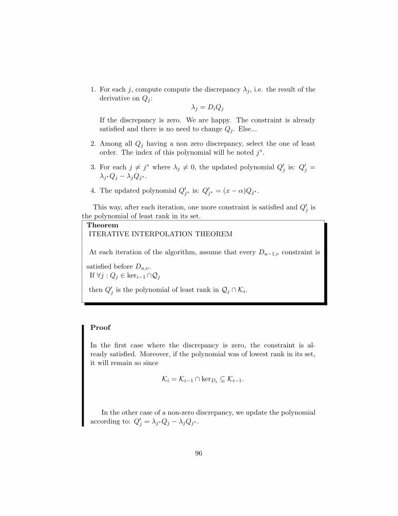
1. For each j, compute compute the discrepancy λj , i.e. the result of thederivative on Qj :

λj = DiQj

If the discrepancy is zero. We are happy. The constraint is alreadysatisfied and there is no need to change Qj . Else...

2. Among all Qj having a non zero discrepancy, select the one of leastorder. The index of this polynomial will be noted j∗.

3. For each j 6= j∗ where λj 6= 0, the updated polynomial Q′j is: Q′j =λj∗Qj − λjQj∗ .

4. The updated polynomial Q′j∗ is: Q′j∗ = (x− α)Qj∗ .

This way, after each iteration, one more constraint is satisfied and Q′j isthe polynomial of least rank in its set.

TheoremITERATIVE INTERPOLATION THEOREM

At each iteration of the algorithm, assume that every Du−1,v constraint is

satisfied before Du,v.If ∀j : Qj ∈ keri−1 ∩Qj

then Q′j is the polynomial of least rank in Qj ∩ Ki.

Proof

In the first case where the discrepancy is zero, the constraint is al-ready satisfied. Moreover, if the polynomial was of lowest rank in its set,it will remain so since

Ki = Ki−1 ∩ kerDi ⊆ Ki−1.

In the other case of a non-zero discrepancy, we update the polynomialaccording to: Q′j = λj∗Qj − λjQj∗ .

96

Since Di is a linear functional and since by hypothesis both Qj andQj∗ belong to Ki−1, it is straightforward that (λj∗Qj − λjQj∗) ∈ Ki−1.Moreover:

Di(λj∗Qj − λjQj∗) = λj∗DiQj − λjDiQj∗ = λj∗λj − λjλj∗ = 0.

Thus Q′j ∈ Ki−1 ∩ kerDi = Ki. Additionally, the rank of Q′j has notchanged since a polynomial of lower rank has been subtracted. Thus ifQj was of lowest rank in its set, it will remain so since Ki ⊆ Ki−1.

The last point is a little more complicated. The lowest ranked poly-nomial Qj∗ is updated by multiplying it by (x− α). Again, it is obviousthat Q′j∗ ∈ Ki−1. But is it also in kerDi? Here comes in play the conditionon constraints ordering that we omitted previously.

DiQ =d

dxDu−1,v(x− λj∗)Qj∗ = Du−1,vQj∗ + (x− α)Du,vQj∗

When evaluating the latter expression at (α, β), the equality becomes:

Du,v(x− λj∗)Qj∗ |(α,β) = Du−1,vQj∗ |ab

Thus, if the constraint constraint Du−1,vQ(x, y)|(α,β) is already satisfied,before DiQ = Du,vQ(x, y)|(α,β) = 0 and is therefore in kerDi , else notnecessarily.

ENDTo summarize it, after the ith iteration, every polynomial Qj is the

lowest rank polynomial in Ki ∩Qj . Thus, at the end of the algorithm, aftera number of iterations equal to the cost of M , the Qj obtained satisfy all theconstraints. Notice that the union of all Qj sets is the set of all polynomialswith y-degree less than or equal to L. The lowest ranked among the Qjpolynomials is therefore also the lowest ranked possible from the whole setof polynomials with y-degree less than or equal to L.

ExampleLet us work over F5 with α = (1, 2) and k = 4. Let the multiplicity matrixbe:

M =(

0 0 0 0 12 0 0 0 0

).

97

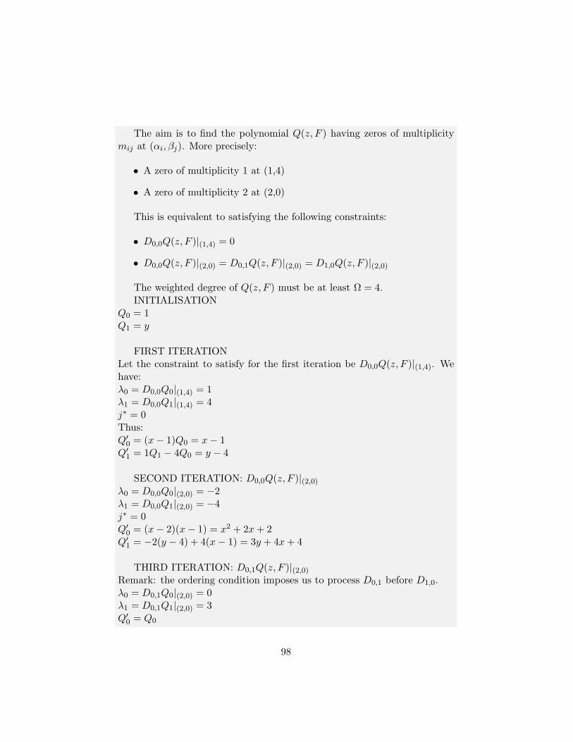
The aim is to find the polynomial Q(z, F ) having zeros of multiplicitymij at (αi, βj). More precisely:

• A zero of multiplicity 1 at (1,4)

• A zero of multiplicity 2 at (2,0)

This is equivalent to satisfying the following constraints:

• D0,0Q(z, F )|(1,4) = 0

• D0,0Q(z, F )|(2,0) = D0,1Q(z, F )|(2,0) = D1,0Q(z, F )|(2,0)

The weighted degree of Q(z, F ) must be at least Ω = 4.INITIALISATION

Q0 = 1Q1 = y

FIRST ITERATIONLet the constraint to satisfy for the first iteration be D0,0Q(z, F )|(1,4). Wehave:λ0 = D0,0Q0|(1,4) = 1λ1 = D0,0Q1|(1,4) = 4j∗ = 0Thus:Q′0 = (x− 1)Q0 = x− 1Q′1 = 1Q1 − 4Q0 = y − 4

SECOND ITERATION: D0,0Q(z, F )|(2,0)

λ0 = D0,0Q0|(2,0) = −2λ1 = D0,0Q1|(2,0) = −4j∗ = 0Q′0 = (x− 2)(x− 1) = x2 + 2x+ 2Q′1 = −2(y − 4) + 4(x− 1) = 3y + 4x+ 4

THIRD ITERATION: D0,1Q(z, F )|(2,0)

Remark: the ordering condition imposes us to process D0,1 before D1,0.λ0 = D0,1Q0|(2,0) = 0λ1 = D0,1Q1|(2,0) = 3Q′0 = Q0

98

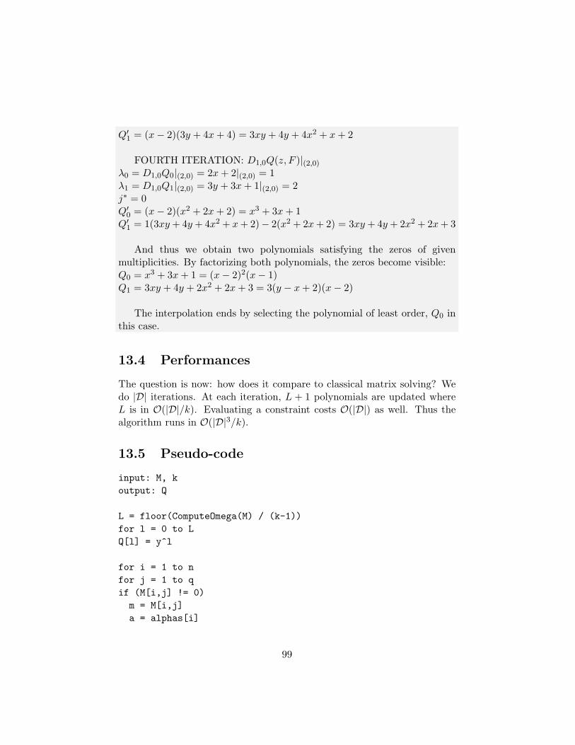
Q′1 = (x− 2)(3y + 4x+ 4) = 3xy + 4y + 4x2 + x+ 2

FOURTH ITERATION: D1,0Q(z, F )|(2,0)

λ0 = D1,0Q0|(2,0) = 2x+ 2|(2,0) = 1λ1 = D1,0Q1|(2,0) = 3y + 3x+ 1|(2,0) = 2j∗ = 0Q′0 = (x− 2)(x2 + 2x+ 2) = x3 + 3x+ 1Q′1 = 1(3xy + 4y + 4x2 + x+ 2)− 2(x2 + 2x+ 2) = 3xy + 4y + 2x2 + 2x+ 3

And thus we obtain two polynomials satisfying the zeros of givenmultiplicities. By factorizing both polynomials, the zeros become visible:Q0 = x3 + 3x+ 1 = (x− 2)2(x− 1)Q1 = 3xy + 4y + 2x2 + 2x+ 3 = 3(y − x+ 2)(x− 2)

The interpolation ends by selecting the polynomial of least order, Q0 inthis case.

13.4 Performances

The question is now: how does it compare to classical matrix solving? Wedo |D| iterations. At each iteration, L + 1 polynomials are updated whereL is in O(|D|/k). Evaluating a constraint costs O(|D|) as well. Thus thealgorithm runs in O(|D|3/k).

13.5 Pseudo-code

input: M, koutput: Q

L = floor(ComputeOmega(M) / (k-1))for l = 0 to LQ[l] = y^l

for i = 1 to nfor j = 1 to qif (M[i,j] != 0)

m = M[i,j]a = alphas[i]

99

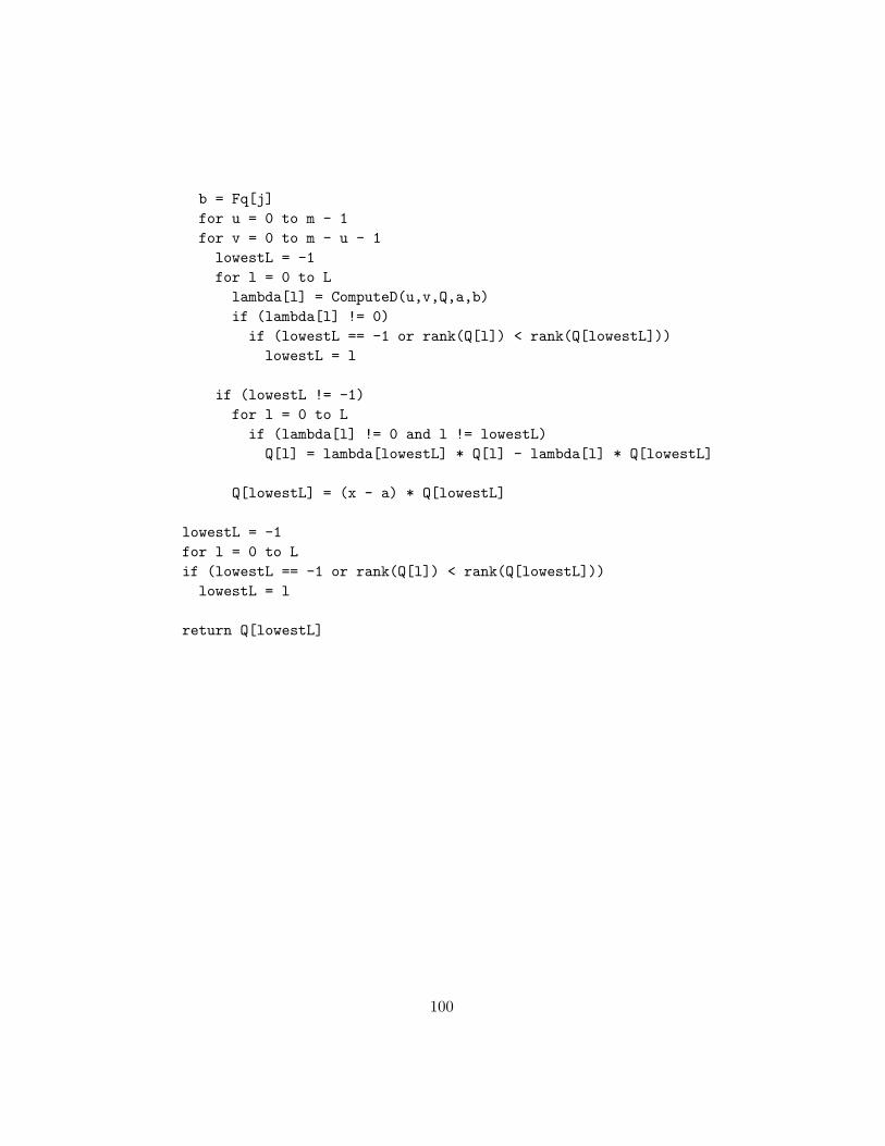
b = Fq[j]for u = 0 to m - 1for v = 0 to m - u - 1lowestL = -1for l = 0 to L

lambda[l] = ComputeD(u,v,Q,a,b)if (lambda[l] != 0)if (lowestL == -1 or rank(Q[l]) < rank(Q[lowestL]))lowestL = l

if (lowestL != -1)for l = 0 to L

if (lambda[l] != 0 and l != lowestL)Q[l] = lambda[lowestL] * Q[l] - lambda[l] * Q[lowestL]

Q[lowestL] = (x - a) * Q[lowestL]

lowestL = -1for l = 0 to Lif (lowestL == -1 or rank(Q[l]) < rank(Q[lowestL]))lowestL = l

return Q[lowestL]

100

Chapter 14

Factorization

In this chapter, we investigate how to find the factors of the type (y− f(x))in Q(x, y). More specifically, only the factors with f(x) of degree less than k.The brute force method would be to test whether f(x) is a y-root of Q(x, y)or not for each polynomial f(x). But of course, this would be outrageouslyexpensive in terms of computation time. For the same price, one coulddirectly test the best candidate among all possible codewords. This is ofcourse unreasonable and we therefore need an efficient algorithm running inpolynomial time.

The one we shall present here is known as the Roth-Ruckenstein factor-ization algorithm, named after its inventors [13].

14.1 Roth-Ruckenstein factorization

Like in the interpolation algorithm, the idea here is not to get all at oncebut the opposite. It is to find out the coefficients of the polynomials one byone. Let us express a polynomial f(x) as:

f(x) = f0 + f1x+ f2x2 + ...

Assume f(x) is a y-root of Q(x, y) so that Q(x, f(x)) = 0. By instantiatingx to 0, we have f(0) = f0 and also that Q(0, f0) = 0. In other words, itmeans that f0 is a y-root of Q(0, y).

Definition 41 Let 〈〈Q(x, y)〉〉 be the normalized polynomial defined as fol-lows:

〈〈Q(x, y)〉〉 = Q(x, y)/xm

where m is the greatest integer such that xm|Q(x, y).

101

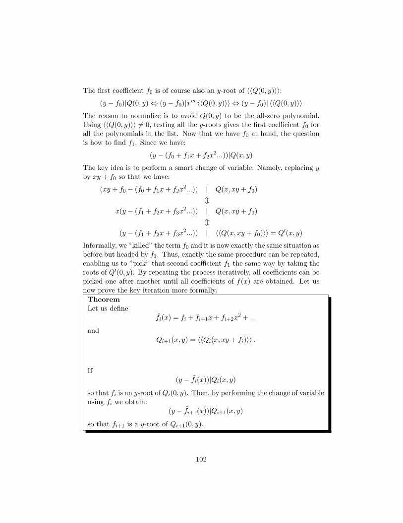
The first coefficient f0 is of course also an y-root of 〈〈Q(0, y)〉〉:

(y − f0)|Q(0, y)⇔ (y − f0)|xm 〈〈Q(0, y)〉〉 ⇔ (y − f0)| 〈〈Q(0, y)〉〉

The reason to normalize is to avoid Q(0, y) to be the all-zero polynomial.Using 〈〈Q(0, y)〉〉 6= 0, testing all the y-roots gives the first coefficient f0 forall the polynomials in the list. Now that we have f0 at hand, the questionis how to find f1. Since we have:

(y − (f0 + f1x+ f2x2...))|Q(x, y)

The key idea is to perform a smart change of variable. Namely, replacing yby xy + f0 so that we have:

(xy + f0 − (f0 + f1x+ f2x2...)) | Q(x, xy + f0)

mx(y − (f1 + f2x+ f3x

2...)) | Q(x, xy + f0)m

(y − (f1 + f2x+ f3x2...)) | 〈〈Q(x, xy + f0)〉〉 = Q′(x, y)

Informally, we ”killed” the term f0 and it is now exactly the same situation asbefore but headed by f1. Thus, exactly the same procedure can be repeated,enabling us to ”pick” that second coefficient f1 the same way by taking theroots of Q′(0, y). By repeating the process iteratively, all coefficients can bepicked one after another until all coefficients of f(x) are obtained. Let usnow prove the key iteration more formally.

TheoremLet us define

fi(x) = fi + fi+1x+ fi+2x2 + ...

andQi+1(x, y) = 〈〈Qi(x, xy + fi)〉〉 .

If(y − fi(x))|Qi(x, y)

so that fi is an y-root of Qi(0, y). Then, by performing the change of variableusing fi we obtain:

(y − fi+1(x))|Qi+1(x, y)

so that fi+1 is a y-root of Qi+1(0, y).

102

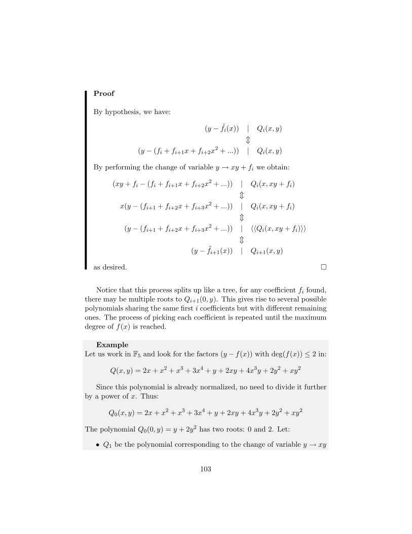
Proof

By hypothesis, we have:

(y − fi(x)) | Qi(x, y)m

(y − (fi + fi+1x+ fi+2x2 + ...)) | Qi(x, y)

By performing the change of variable y → xy + fi we obtain:

(xy + fi − (fi + fi+1x+ fi+2x2 + ...)) | Qi(x, xy + fi)

mx(y − (fi+1 + fi+2x+ fi+3x

2 + ...)) | Qi(x, xy + fi)m

(y − (fi+1 + fi+2x+ fi+3x2 + ...)) | 〈〈Qi(x, xy + fi)〉〉

m(y − fi+1(x)) | Qi+1(x, y)

as desired.

Notice that this process splits up like a tree, for any coefficient fi found,there may be multiple roots to Qi+1(0, y). This gives rise to several possiblepolynomials sharing the same first i coefficients but with different remainingones. The process of picking each coefficient is repeated until the maximumdegree of f(x) is reached.

ExampleLet us work in F5 and look for the factors (y− f(x)) with deg(f(x)) ≤ 2 in:

Q(x, y) = 2x+ x2 + x3 + 3x4 + y + 2xy + 4x3y + 2y2 + xy2

Since this polynomial is already normalized, no need to divide it furtherby a power of x. Thus:

Q0(x, y) = 2x+ x2 + x3 + 3x4 + y + 2xy + 4x3y + 2y2 + xy2

The polynomial Q0(0, y) = y + 2y2 has two roots: 0 and 2. Let:

• Q1 be the polynomial corresponding to the change of variable y → xy

103

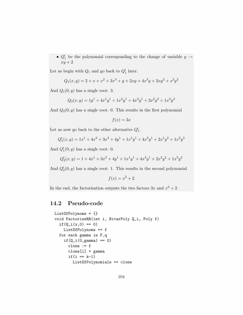
• Q′1 be the polynomial corresponding to the change of variable y →xy + 2

Let us begin with Q1 and go back to Q′1 later.

Q1(x, y) = 2 + x+ x2 + 3x3 + y + 2xy + 4x3y + 2xy2 + x2y2

And Q1(0, y) has a single root: 3.

Q2(x, y) = 1y1 + 4x1y1 + 1x2y1 + 4x3y1 + 2x2y2 + 1x3y2

And Q2(0, y) has a single root: 0. This results in the first polynomial

f(x) = 3x

Let us now go back to the other alternative Q′1.

Q′1(x, y) = 1x1 + 4x2 + 3x3 + 4y1 + 1x1y1 + 4x3y1 + 2x1y2 + 1x2y2

And Q′1(0, y) has a single root: 0.

Q′2(x, y) = 1 + 4x1 + 3x2 + 4y1 + 1x1y1 + 4x3y1 + 2x2y2 + 1x3y2

And Q′2(0, y) has a single root: 1. This results in the second polynomial

f(x) = x2 + 2

In the end, the factorization outputs the two factors 3x and x2 + 2.

14.2 Pseudo-code

ListOfPolynoms = void FactorizeRR(int i, BivarPoly Q_i, Poly f)

if(Q_i(x,0) == 0)ListOfPolynoms += f

for each gamma in F_qif(Q_i(0,gamma) == 0)

clone := fclone[i] = gammaif(i == k-1)ListOfPolynomials += clone

104

elseQ_i_next += Normalize(Q_i(x, xy + gamma))FactorizeRR(i+1 , Q_i_next, clone)

105

Chapter 15

Program notes

In this chapter, we present the source code provided along with this text.It tells what the API provides, how to use it and a few implementationnotes. This includes examples of code excerpts to demonstrate how to usethe API. The program is primarily written for educational purposes, toillustrate how the algorithm works, to experiment with the algebraic soft-decoding and to see it in action. Besides of this, it provides also a limitedAPI that can be used for performing computation with polynomials in finitefields, implementing encoders, decoders and other communication systemcomponents. Lastly, it can also be used to provide benchmarks. Despitethe program favors clarity in spite of performances, these ones should beacceptable and have the same running time asymptotic properties as in thetheory. The language C# was chosen because of several reasons: it is wellknown, it is relatively efficient, it is multi-platform (in theory at least...)and lastly it offers operator overloading which increases a lot readability aswell as comfort when writing and using the source code.

As a side note, a free IDE called visual C# express is provided by Mi-crosoft. This IDE can be downloaded freely on the net, is extremely easy toset up and getting the source code running is just a matter of minutes.

The program can be divided in four main parts:

• Algebra tools: classes for finite fields and polynomials over such fields

• Communication system: interfaces for encoders, channels and decoders

• Channel models: the different kind of channel models implemented

• Reed-Solomon: encoders and decoders for Reed-Solomon codes

106

15.1 Algebra

15.1.1 Finite fields

Two kinds of finite fields are currently implemented: prime fields and fieldswhose size are a power of two. Their source code is in PrimeField.csand BinaryExtensionField.cs respectively. A finite field element is rep-resented externally by the struct FFE, the choice of being a struct andnot an object is for performance reasons. Internally, the finite field elementis represented by an integer for performance reasons as well. For extensionfields Fpm , the following bijection to integers Fpm ↔ N is used:

a0 + a1x+ ...+ amxm ⇔

m∑i=0

aipi

Both classes are written in order to take advantage of the structure ofthe field for these sizes. For example, for fields whose size is a power of 2,bitwise addition is performed directly whereas modular arithmetic is usedin prime fields. All operations are in O(1). In fields whose size is a powerof 2, primitive polynomials are hard-coded and enable to make fields of sizeup to 216.

And now a few example. To construct a field:

FiniteField Fq = new PrimeField(101); // q = p = 101FiniteField Fq = new BinaryExtensionField(8); // q = 2^8 = 1024

To get elements of a field:

FFE a = Fq[3];FFE b = Fq[47];

To perform computations in fields:

FFE result = a * Fq[21] + b / Fq[33] + (Fq[2]^3402);Console.WriteLine(result);

The reason the exponent has been put in parenthesis is that this operatorin C# initially stands for bitwise XOR and has no precedence over otheroperators.

Remark: since FFE is a struct, it is created by default upon declara-tion with all fields uninitialized. Doing so results in broken field elements.myFiniteField[i] should always be used to get elements.

A prime extenstion field class can be implemented and seamlessly inte-grated in the API provided it implements the FiniteField interface.

107

15.2 Polynomials

To be more precise, bivariate polynomials. Polynomials of different degreesin x,y can be added, subtracted, multiplied and powers of them can betaken. Except for polynomial powers, all other operations are efficientlyimplemented. The next few code lines illustrates how polynomials can beused.

// Let Fq = FFE.DEFAULT_FIELDPolynomial p = new Polynomial(new int[,]0,3,0,0,0,2); // result: p(x,y) = Fq[3]y + Fq[2] xy^2Polynomial q = new Polynomial(4,3); // a polynomial whose max x-degree is 4 and max y-degree is 3q[3,3] = Fq[5]; // result: q(x,y) = Fq[5]x^3y^3

Console.WriteLine((p*q - Fq[21]*p)^2);

Polynomial poly = Fq[1]; // implicit conversionPolynomial x = Polynomial.GetX();

for(int i=0; i<Fq.q; i++)poly = poly * (x - Fq[i]);

Console.WriteLine(poly); // prints x^q - x

Internally, polynomials store an array of FFE being the coefficients of thepowers of x and y.

15.3 Communication System

15.3.1 Interfaces

The communication system is represented by three key interfaces which areutterly simple.

• Encoder: any encoder must implement this interface which consists ofthe single method FFE[] Encode(FFE[] message).

• Channel: any channel must implement this interface which consists oftwo methods:

– void Send(FFE[] word)

– double[,] Receive(): returns the reliability matrix for the lastsent word

108

• FFE[] Decode(double[,] RM): given the reliability matrix as input,perform the decoding algorithm. For hard-decoding, the auxiliarymethod FFE[] GetQuantizedReceivedWord(double[,] RM) can beused.

By means of these interfaces, various components can be put togetherto form the system. Moreover, it is easy to extend the current programby adding different kind of channels, other decoders and so on. That way,running simulation in a standardized way becomes easy:

FiniteField Fq = new MyFiniteField(...);

Encoder encoder = new MyEncoder(...);Channel channel = new MyChannel(...);Decoder decoder = new MyDecoder(...);

for (int i = 0; i < howManyTimes; i++)FFE[] m = RandomMessage();FFE[] x = encoder.Encode(m);channel.Send(x);double[,] RM = channel.Receive();FFE[] hatx = decoder.Decode(RM);

15.3.2 Channels

Three channels are implemented:

• a noiseless channel outputting the same as is sent.

• a Qary symmetric channel with custom transition probabilities.

• a ”binary extension channel” explained next.

The last channel works only for the transmission of symbols from afinite field whose size is 2m for some m. Each symbol is mapped onto bits,transmitted an underlying binary symmetric channel of crossover probabilityperr, then the received sequence of bits is mapped back to the symbol itstands for. The probability that β was sent if γ is received depends on thenumber of locations in which bits differ, noted be:

p(X = β|Y = γ) = pbeerr(1− perr)m−be

109

ExampleLet m = 4 and perr = 0.1 and assume that 1100 is received. Then:

• 1100 has a probability of 0.94 of being the sent symbol.

• 1000, 0100, 111, 1101 have each a probability of 0.1 ∗ 0.93 of being thesent symbol.

• ...

• 0011 has a probability of 0.14 of being the sent symbol.

15.3.3 Encoders and decoders

A Reed-Solomon encoder is implemented. It works for any finite field andany valid parameters. The locations where the encoding polynomial is evalu-ated can be specified or chosen by default. Two decoders were implemented:

• A bounded-distance hard-decoder performing the Gao algorithm pre-sented in chapter 7 and decoding up to n−k

2 errors.

• The algebraic soft-decoder for Reed-Solomon codes described in thisthesis. It uses the greedy MAA with the number of total multiplicitiesis given, the Kotter interpolation and the Roth-Ruckenstein factoriza-tion.

In the first line of the source code of RSSoftDecoder.cs are preprocessordirectives included to indicate if the algorithm should execute in normal,verbose or mute mode.

• In the verbose mode, every step is printed on the screen with everytemporary polynomial obtained during the interpolation and factor-ization steps.

• In the normal mode, a dot is printed each time a constraint is satisfiedduring the interpolation. Once interpolation has finished, the resultingpolynomial is printed. For factorization, a dot is printed for each rootfound and upon termination the list of potential encoding polynomialsfound are printed.

• In the mute mode, nothing at all is printed.

Code to run tests directly can be found in Benchmark.cs.

110

Chapter 16

Conclusion

In practice, the advantage of this algebraic soft decoding algorithm dependson:

• the rate of the code

• the kind of channel

• the available computational power

Since the rate of a code is directly chosen depending on the magnitudeof the noise in the channel (for low noise, high code rates are used and vice-versa), these two arguments in fact boil down to the same one. Both forlow rate codes and for very noisy channels, this algorithm offers tremendousbenefits. Unfortunately, neither of these situations are frequent in practice.For example, optical fiber has crossover probabilities in the range of 10−12,CD-Roms use RS codes with parameters k = 239 and n = 255, and so on.For these higher rate codes and low noise channels, the benefits are lower andmore expensive (computationally) but nevertheless present. If the systemcan afford these computational resources, this alternative should be takeninto account.

Another advantage for this algorithm is that it can easily be fined tunedbetween performances in decoding ability and rapidity of execution. Indeed,both are directly dependent on the number of interpolation points.

Despite it does not look very attractive for the moment at high rates,some very promising improvements for this algorithm emerged during thelast few years. Here are some of them:

111

• There is the fact that it can be extended for soft-decoding algebraicgeometry codes which are superior to RS codes.

• In [10][11], four authors show the equivalence between the initial in-terpolation problem and a transformed interpolation problem of lessercomplexity by means of a genuine change of variable. The transformedinterpolation problem has the property that a significant amount ofconstraints can be pre-solved. This reduces the number of constraintsin the shifted interpolation problem by at least n

n−k .

• El-Khamy and McEliece showed a better optimization problem forthe assignment of the multiplicity matrix providing an MAA leadingto greatly improved error correcting ability [15].

• In [17], Guruswami and Rudra showed that by carefully selection thelocations at which the Reed-Solomon is evaluated, cyclic errors upto the capacity can be corrected. He calls this folded Reed-Solomoncodes and takes advantage of relation between polynomials evaluatedat specified locations.

• Iterative algorithms to perform the interpolation while giving the in-termediate results to be factored are being developed.

• Lastly, some papers go toward an implementation of this algorithm onan electronic level with VLSI.

Combining these recent advances together, it would not be surprising tohave significantly increased decoding performances while having a significantreduction in computational complexity. This would make this decodingalgorithm also attractive at high rates. It is surely only a matter of timeuntil they are applied in practice.

112

Bibliography

[1] The Theory of Error-Correcting Codes- F.J. MacWilliams and N.J.A. SloaneNorth-Holland, Amsterdam, 1977, 762 pp.

[2] Lecture notes- J. Hallhttp://www.mth.msu.edu/~jhall/classes/codenotes/coding-notes.html

[3] A new algorithm for decoding Reed-Solomon codes- S. GaoCommunications, Information and Network Security (V. Bhargava, H.V. Poor, V. Tarokh and S. Yoon, Eds.), Kluwer Academic Publishers,2003, p. pp. 55–68http://www.math.clemson.edu/faculty/Gao/papers/RS.pdf

[4] A Mathematical Theory of Communication- C. Shannonhttp://cm.bell-labs.com/cm/ms/what/shannonday/shannon1948.pdfThe Bell System Technical Journal, Vol. 27, pp. 379-423, 623-656, July,October, 1948

[5] Decoding of Reed-Solomon codes beyond the error-correction bound- M. SudanJournal of Complexity, 13(1): 180–193, March 1997http://people.csail.mit.edu/madhu/papers/reeds-journ.ps

[6] Improved decoding of Reed-Solomon and algebraic-geometry codes- V. Guruswami, M. SudanIEEE Transactions on Information Theory, 45(6): 1757–1767, Septem-ber 1999.http://people.csail.mit.edu/madhu/papers/venkat-journ.ps

113

[7] Reflections on ”Improved decoding of Reed-Solomon and algebraic-geometry codes”- V. Guruswami, M. SudanIEEE Information Theory Society Newsletter, Volume 52, Number 1,ISSN 1059-2362, pages 6-12, March 2002.http://people.csail.mit.edu/madhu/papers/reflections.ps

[8] The Guruswami-Sudan Decoding Algorithm for Reed-Solomon Codes.- R. J. McElieceThe Interplanetary Network Progress Report, IPN PR 42-153, January-March 2003, pp. 1-60http://tmo.jpl.nasa.gov/progress report/42-153/153F.pdf

[9] Algebraic soft-decision decoding of Reed-Solomon codes- R. Koetter, A. VardyIEEE Transactions on Information Theory, vol. 49, no. 11, November2003http://www.eecs.berkeley.edu/~dolecek/coding/KoetterVardy03.pdf

[10] Efficient interpolation and factorization in algebraic soft-decision de-coding of Reed-Solomon codes- R. Koetter, J. Ma, A. Vardy, and A. Ahmed

[11] A Complexity Reducing Transformation in Algebraic List Decoding ofReed-Solomon Codes- Ralf Koetter, Alexander Vardy

[12] Fast Generalized Minimum Distance Decoding of Algebraic-Geometryand Reed-Solomon Codes- R. KotterIEEE Transaction in Information Theory, vol. 42, no. 3, pp. 721-737,May 1996

[13] Efficient Decoding of Reed-Solomon Codes beyond Half the MinimumDistance- R. Roth and G. RuckensteinTrans. Info. Theory, vol. 46, no. 1, pp. 246256, Jan. 2000

[14] Algebraic Soft-Decision Decoding of Reed-Solomon Codes Using Bit-level Soft Information- Jing Jiang and Krishna R. Narayanan

114

in Proc. Allerton Conference on Communications, Control and Com-puting 2006 and submitted to IEEE Trans. on Information Theory.http://www.ece.tamu.edu/~jjiang/bit gmd.pdf

[15] Interpolation Multiplicity Assignment Algorithms for Algebraic Soft-Decision Decoding of Reed Solomon CodesM. El-Khamy and R. J. McElieceAMS-DIMACS volume on Algebraic Coding Theory and InformationTheory, vol. 68, 2005.http://www.its.caltech.edu/~mostafa/pubs/DimacsElk8c.pdf

[16] Codes and Curves- Judy L. Walkerexpository monograph, published by the AMS in the IAS/Park CityMathematical Subseries of the Student Mathematical Series.http://www.math.unl.edu/~jwalker7/papers/rev.pdf

[17] Achieving List Decoding Capacity Using Folded Reed-Solomon Codes- V. Guruswami and A. RudraInvited paper at Allerton 2006http://www.cs.washington.edu/homes/venkat/pubs/papers/FRS-allerton.pdf

[18] Iterative Algebraic Soft-Decision List Decoding of Reed-Solomon Codes- M. El-Khamy. and R. J. McEliecehttp://arxiv.org/PS cache/cs/pdf/0509/0509097v1.pdf

[19] aximum-Likelihood Decoding of Reed-Solomon Codes is NP-hardV. Guruswami and A. VardySODA 2005; accepted to IEEE Trans. Info. Theoryhttp://www.cs.washington.edu/homes/venkat/pubs/papers/mldrs.pdf

115

Part III

Appendix

116

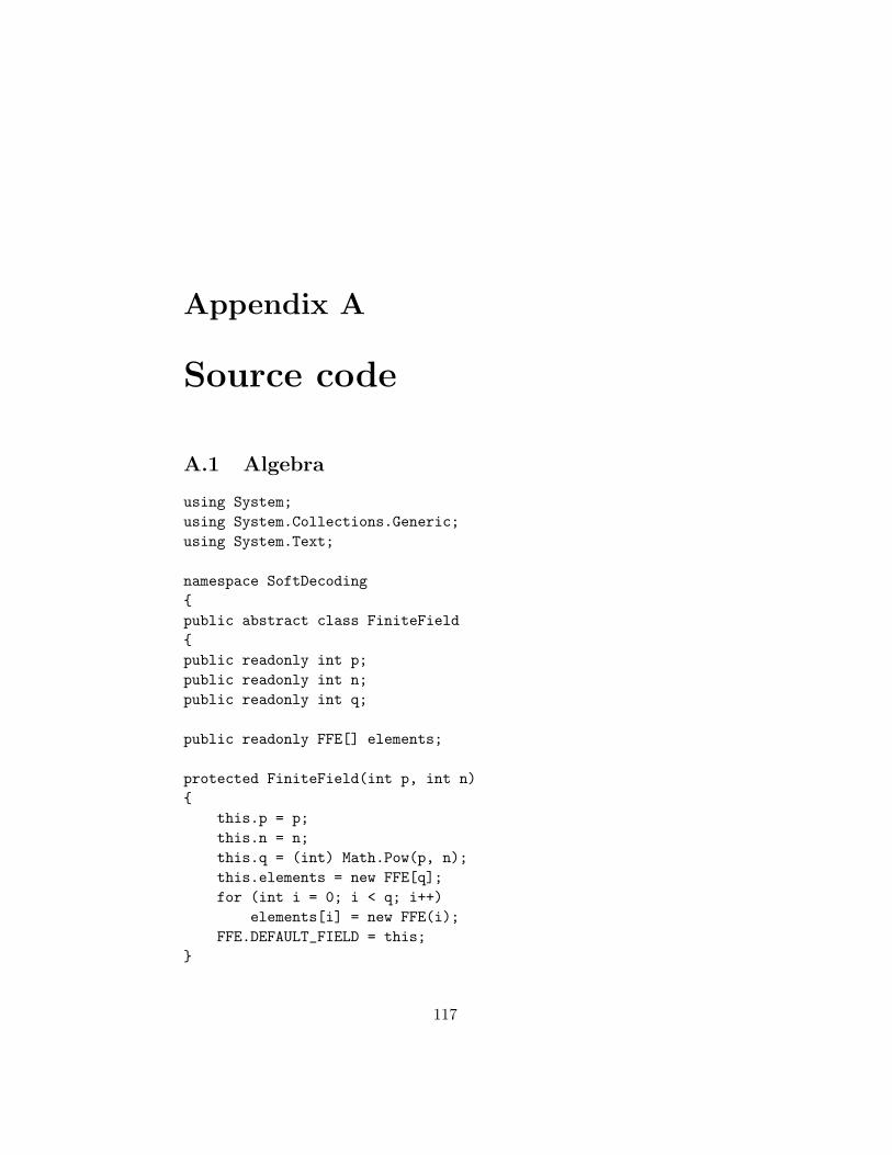
Appendix A

Source code

A.1 Algebra

using System;using System.Collections.Generic;using System.Text;

namespace SoftDecodingpublic abstract class FiniteFieldpublic readonly int p;public readonly int n;public readonly int q;

public readonly FFE[] elements;

protected FiniteField(int p, int n)

this.p = p;this.n = n;this.q = (int) Math.Pow(p, n);this.elements = new FFE[q];for (int i = 0; i < q; i++)

elements[i] = new FFE(i);FFE.DEFAULT_FIELD = this;

117

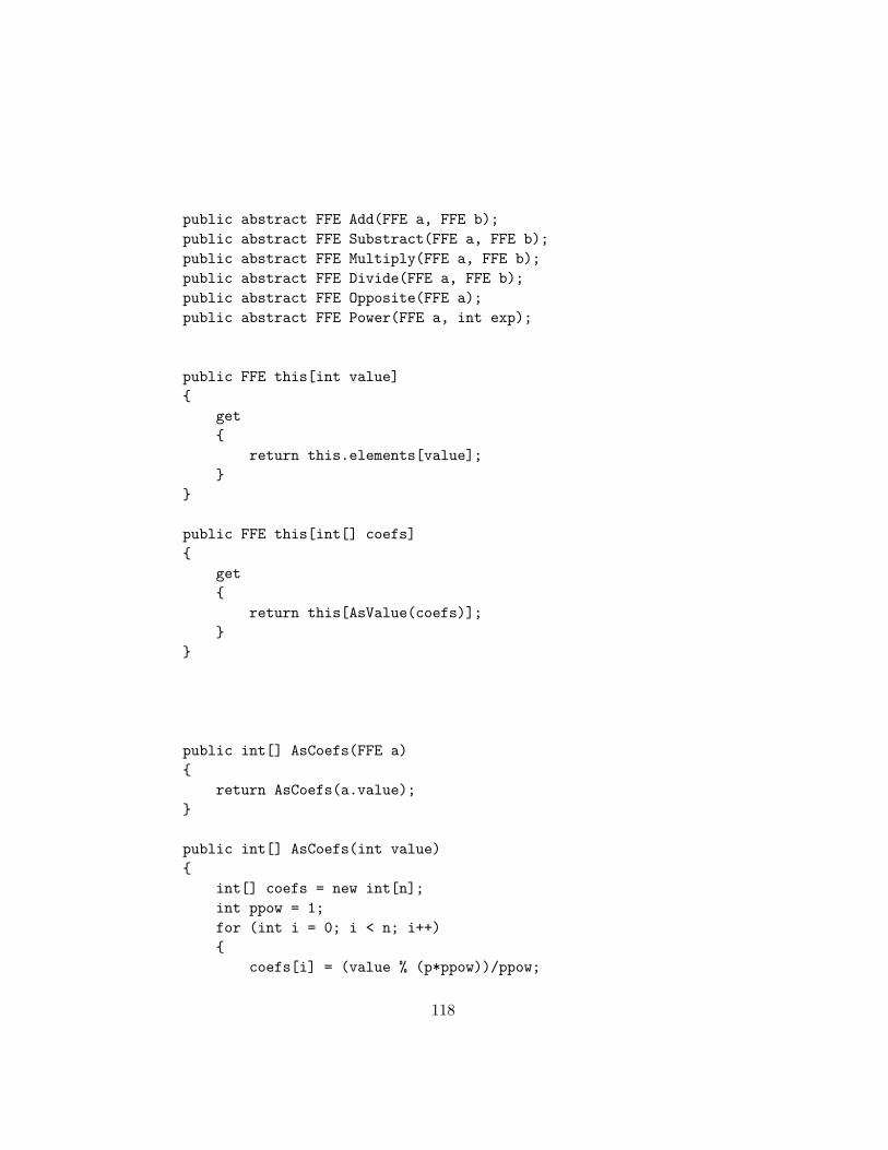
public abstract FFE Add(FFE a, FFE b);public abstract FFE Substract(FFE a, FFE b);public abstract FFE Multiply(FFE a, FFE b);public abstract FFE Divide(FFE a, FFE b);public abstract FFE Opposite(FFE a);public abstract FFE Power(FFE a, int exp);

public FFE this[int value]

get

return this.elements[value];

public FFE this[int[] coefs]

get

return this[AsValue(coefs)];

public int[] AsCoefs(FFE a)

return AsCoefs(a.value);

public int[] AsCoefs(int value)

int[] coefs = new int[n];int ppow = 1;for (int i = 0; i < n; i++)

coefs[i] = (value % (p*ppow))/ppow;

118

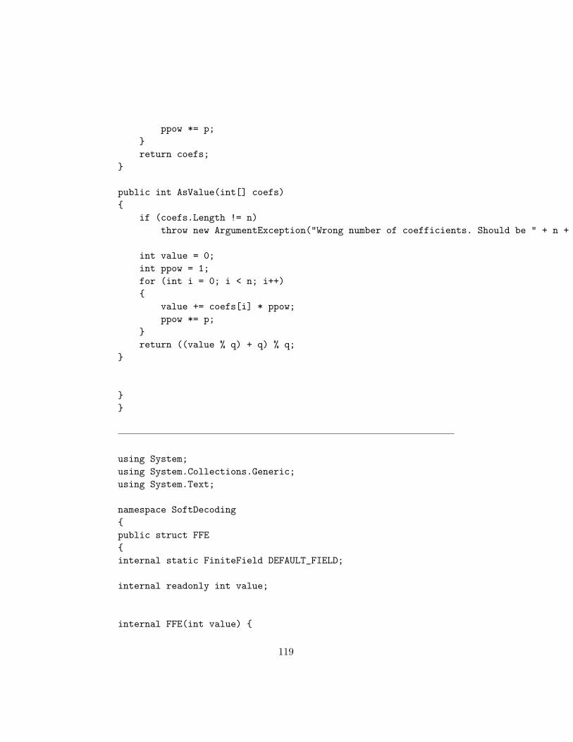
ppow *= p;return coefs;

public int AsValue(int[] coefs)

if (coefs.Length != n)throw new ArgumentException("Wrong number of coefficients. Should be " + n + " instead of " + coefs.Length + ".");

int value = 0;int ppow = 1;for (int i = 0; i < n; i++)

value += coefs[i] * ppow;ppow *= p;

return ((value % q) + q) % q;

using System;using System.Collections.Generic;using System.Text;

namespace SoftDecodingpublic struct FFEinternal static FiniteField DEFAULT_FIELD;

internal readonly int value;

internal FFE(int value)

119

this.value = value;

public override String ToString() if (DEFAULT_FIELD.n == 1)

return this.value.ToString();else

String ans = "";int[] coefs = DEFAULT_FIELD.AsCoefs(value);for (int i = 0; i < coefs.Length; i++)

ans += coefs[i];return ans;/*if (this.value == 0)

return "X";

for (int i = 0; i < DEFAULT_FIELD.q; i++)

int power = (DEFAULT_FIELD[2] ^ i).value;if (this.value == power)

return i.ToString();

throw new Exception("Field element is not the power of the generator element.");*/

public static FFE operator +(FFE a, FFE b) return DEFAULT_FIELD.Add(a, b);

public static FFE operator -(FFE a) return DEFAULT_FIELD.Opposite(a);

120

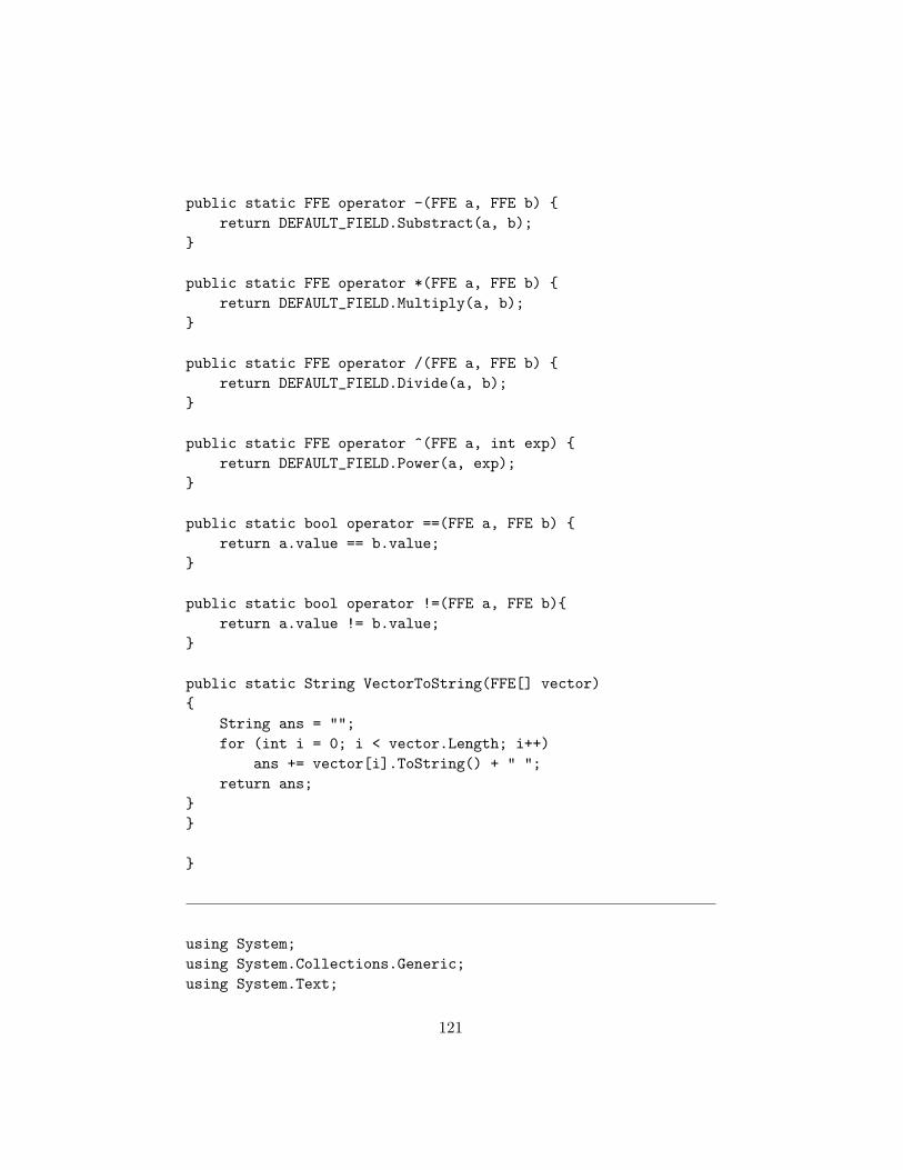
public static FFE operator -(FFE a, FFE b) return DEFAULT_FIELD.Substract(a, b);

public static FFE operator *(FFE a, FFE b) return DEFAULT_FIELD.Multiply(a, b);

public static FFE operator /(FFE a, FFE b) return DEFAULT_FIELD.Divide(a, b);

public static FFE operator ^(FFE a, int exp) return DEFAULT_FIELD.Power(a, exp);

public static bool operator ==(FFE a, FFE b) return a.value == b.value;

public static bool operator !=(FFE a, FFE b)return a.value != b.value;

public static String VectorToString(FFE[] vector)

String ans = "";for (int i = 0; i < vector.Length; i++)

ans += vector[i].ToString() + " ";return ans;

using System;using System.Collections.Generic;using System.Text;

121

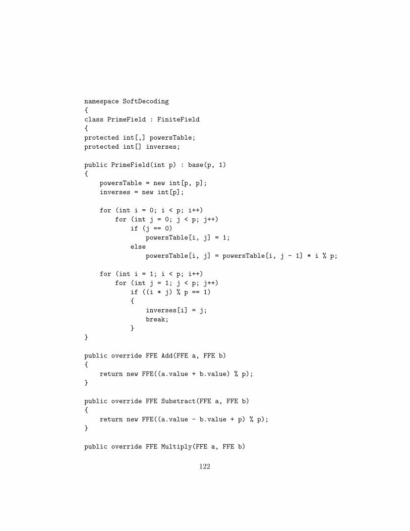
namespace SoftDecodingclass PrimeField : FiniteFieldprotected int[,] powersTable;protected int[] inverses;

public PrimeField(int p) : base(p, 1)

powersTable = new int[p, p];inverses = new int[p];

for (int i = 0; i < p; i++)for (int j = 0; j < p; j++)

if (j == 0)powersTable[i, j] = 1;

elsepowersTable[i, j] = powersTable[i, j - 1] * i % p;

for (int i = 1; i < p; i++)for (int j = 1; j < p; j++)

if ((i * j) % p == 1)

inverses[i] = j;break;

public override FFE Add(FFE a, FFE b)

return new FFE((a.value + b.value) % p);

public override FFE Substract(FFE a, FFE b)

return new FFE((a.value - b.value + p) % p);

public override FFE Multiply(FFE a, FFE b)

122

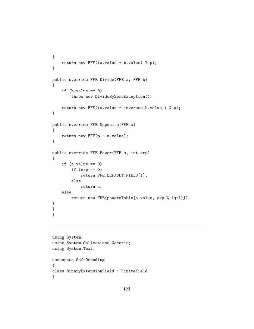
return new FFE((a.value * b.value) % p);

public override FFE Divide(FFE a, FFE b)

if (b.value == 0)throw new DivideByZeroException();

return new FFE((a.value * inverses[b.value]) % p);

public override FFE Opposite(FFE a)

return new FFE(p - a.value);

public override FFE Power(FFE a, int exp)

if (a.value == 0)if (exp == 0)

return FFE.DEFAULT_FIELD[1];else

return a;else

return new FFE(powersTable[a.value, exp % (q-1)]);

using System;using System.Collections.Generic;using System.Text;

namespace SoftDecodingclass BinaryExtensionField : FiniteField

123

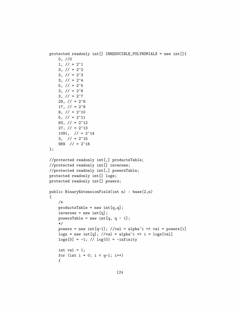
protected readonly int[] IRREDUCIBLE_POLYNOMIALS = new int[]0, //01, // = 2^13, // = 2^23, // = 2^33, // = 2^45, // = 2^53, // = 2^63, // = 2^729, // = 2^817, // = 2^99, // = 2^105, // = 2^1183, // = 2^1227, // = 2^131091, // = 2^143, // = 2^15989 // = 2^16

;

//protected readonly int[,] productsTable;//protected readonly int[] inverses;//protected readonly int[,] powersTable;protected readonly int[] logs;protected readonly int[] powers;

public BinaryExtensionField(int n) : base(2,n)

/*productsTable = new int[q,q];inverses = new int[q];powersTable = new int[q, q - 1];*/powers = new int[q-1]; //val = alpha^i => val = powers[i]logs = new int[q]; //val = alpha^i => i = logs[val]logs[0] = -1; // log(0) = -infinity

int val = 1;for (int i = 0; i < q-1; i++)

124

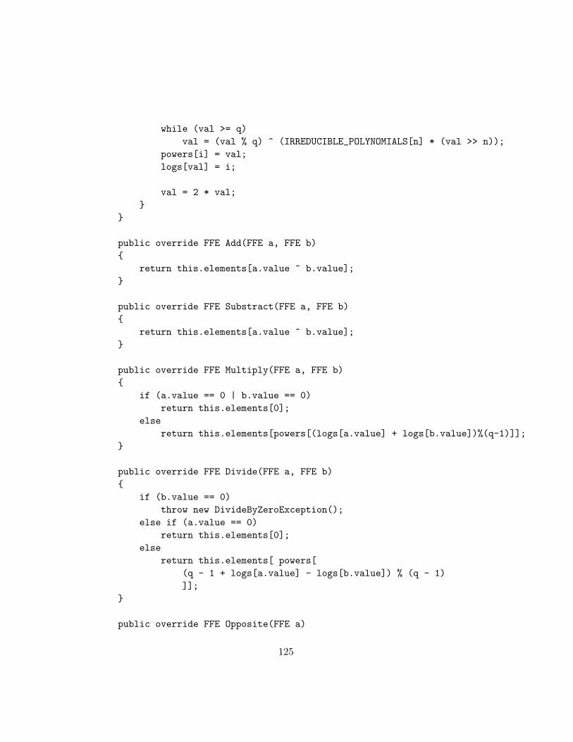
while (val >= q)val = (val % q) ^ (IRREDUCIBLE_POLYNOMIALS[n] * (val >> n));

powers[i] = val;logs[val] = i;

val = 2 * val;

public override FFE Add(FFE a, FFE b)

return this.elements[a.value ^ b.value];

public override FFE Substract(FFE a, FFE b)

return this.elements[a.value ^ b.value];

public override FFE Multiply(FFE a, FFE b)

if (a.value == 0 | b.value == 0)return this.elements[0];

elsereturn this.elements[powers[(logs[a.value] + logs[b.value])%(q-1)]];

public override FFE Divide(FFE a, FFE b)

if (b.value == 0)throw new DivideByZeroException();

else if (a.value == 0)return this.elements[0];

elsereturn this.elements[ powers[

(q - 1 + logs[a.value] - logs[b.value]) % (q - 1)]];

public override FFE Opposite(FFE a)

125

return a;

public override FFE Power(FFE a, int exp)

if (a.value == 0)if (exp == 0)

return this.elements[1];else

return this.elements[0];else

return this.elements[powers[(logs[a.value]* exp) % (q - 1)]];

using System;using System.Collections.Generic;using System.Text;

namespace SoftDecodingstruct Polynomialprivate FFE[,] values;

public FFE this[int i, int j]

get

if (i < values.GetLength(0) & j < values.GetLength(1))return values[i, j];

elsereturn FFE.DEFAULT_FIELD[0];

set

126

if (i < values.GetLength(0) & j < values.GetLength(1))values[i, j] = value;

else

FFE[,] old = values;values = new FFE[Math.Max(i, old.GetLength(0)), Math.Max(j, old.GetLength(1))];for (int ii = 0; ii < old.GetLength(0); ii++)

for (int jj = 0; jj < old.GetLength(1); jj++)values[ii, jj] = old[ii, jj];

values[i, j] = value;

public Polynomial(int[,] values)

this.values = new FFE[values.GetLength(0), values.GetLength(1)];for (int i = 0; i < values.GetLength(0); i++)

for (int j = 0; j < values.GetLength(1); j++)this.values[i, j] = FFE.DEFAULT_FIELD[values[i,j]];

public Polynomial(FFE[,] values)

this.values = values;

public Polynomial(FFE[] values)

this.values = new FFE[values.Length, 1];for (int i = 0; i < values.Length; i++)

this.values[i,0] = values[i];

public static Polynomial GetX()

return new Polynomial(new FFE[,] FFE.DEFAULT_FIELD[0] , FFE.DEFAULT_FIELD[1] );

127

public static Polynomial GetY()

return new Polynomial(new FFE[,] FFE.DEFAULT_FIELD[0], FFE.DEFAULT_FIELD[1] );

public int GetMaxDegX() return values.GetLength(0)-1;

public int GetDegreeX()

for (int i = this.GetMaxDegX(); i >= 0; i--)for (int j = 0; j <= this.GetMaxDegY(); j++)

if (values[i, j] != FFE.DEFAULT_FIELD[0])return i;

return 0;

public int GetMaxDegY()return values.GetLength(1)-1;

public Polynomial(int maxDegX, int maxDegY)

this.values = new FFE[maxDegX+1, maxDegY+1];

public static Polynomial operator +(Polynomial P, Polynomial Q)

Polynomial res = new Polynomial(Math.Max(P.GetMaxDegX(), Q.GetMaxDegX()),Math.Max(P.GetMaxDegY(), Q.GetMaxDegY()));

for (int i = 0; i <= res.GetMaxDegX(); i++)for (int j = 0; j <= res.GetMaxDegY(); j++)

res[i, j] = P[i, j] + Q[i, j];

128

return res;

public static Polynomial operator -(Polynomial P, Polynomial Q)

Polynomial res = new Polynomial(Math.Max(P.GetMaxDegX(), Q.GetMaxDegX()),Math.Max(P.GetMaxDegY(), Q.GetMaxDegY()));

for (int i = 0; i <= res.GetMaxDegX(); i++)for (int j = 0; j <= res.GetMaxDegY(); j++)

res[i, j] = P[i, j] - Q[i, j];

return res;

public static Polynomial operator *(Polynomial P, Polynomial Q)

Polynomial res = new Polynomial(P.GetDegreeX() + Q.GetDegreeX(), P.GetMaxDegY() + Q.GetMaxDegY());

for (int pi = 0; pi <= P.GetDegreeX(); pi++)for (int pj = 0; pj <= P.GetMaxDegY(); pj++)

if(P[pi,pj] != FFE.DEFAULT_FIELD[0])for (int qi = 0; qi <= Q.GetDegreeX(); qi++)

for (int qj = 0; qj <= Q.GetMaxDegY(); qj++)res[pi+qi, pj+qj] += P[pi, pj] * Q[qi, qj];

return res;

public static Polynomial operator ^(Polynomial P, int exp)

if (P == GetX())

Polynomial res = new Polynomial(exp, 0);res[exp,0] = FFE.DEFAULT_FIELD[1];

129

return res;else if (P == GetY())

Polynomial res = new Polynomial(0, exp);res[0, exp] = FFE.DEFAULT_FIELD[1];return res;

else

Polynomial ans = FFE.DEFAULT_FIELD[1];for (int i = 0; i < exp; i++)

ans *= P;return ans;

// implicit conversion from an FFE to a polynomialpublic static implicit operator Polynomial(FFE value)

return new Polynomial(new FFE[,] value );

public FFE Evaluate(FFE xVal, FFE yVal)

FFE res = FFE.DEFAULT_FIELD[0];for (int i = 0; i <= GetMaxDegX(); i++)

for (int j = 0; j <= GetMaxDegY(); j++)res += this.values[i,j]*(xVal^i)*(yVal^j);

return res;

public override string ToString()

130

String ans = "";FFE zero = FFE.DEFAULT_FIELD[0];for (int j = 0; j <= GetMaxDegY(); j++)

for (int i = 0; i <= GetMaxDegX(); i++)if (this[i, j] != zero)

ans += this[i, j] + (i == 0 ? "" : "x^" + i) + (j == 0 ? "" : "y^" + j) + " + ";

if (ans.Length > 0)return ans.Substring(0, ans.Length - 2);

elsereturn "0";

public static bool operator ==(Polynomial P, Polynomial Q)

return !(P != Q);

public static bool operator !=(Polynomial P, Polynomial Q)

int maxDegX = (int) Math.Max(P.GetMaxDegX(), Q.GetMaxDegX());int maxDegY = (int) Math.Max(P.GetMaxDegY(), Q.GetMaxDegY());

for (int i = 0; i <= maxDegX; i++)for (int j = 0; j <= maxDegY; j++)

if (P[i, j] != Q[i, j])return true;

return false;

A.2 Communication system interfaces

using System;

131

using System.Collections.Generic;using System.Text;

namespace SoftDecodinginterface Encoder

FFE[] Encode(FFE[] message);

using System;using System.Collections.Generic;using System.Text;

namespace SoftDecodinginterface Channel

void Send(FFE[] word);double[,] Receive(); // returns the reliability matrix

using System;using System.Collections.Generic;using System.Text;

namespace SoftDecodinginterface Decoder

FFE[] Decode(double[,] RM);

132

A.3 Reed-Solomon encoders/decoders

using System;using System.Collections.Generic;using System.Text;

namespace SoftDecodingclass RSEncoder : Encoderpublic readonly int n;public readonly int k;public readonly FFE[] alphas;

internal RSEncoder(int k, FFE[] alphas)

this.n = alphas.Length;this.k = k;this.alphas = alphas;

public static FFE[] GetDefautLocation(FiniteField Fq, int n)

if (n > Fq.q)throw new ArgumentException("More locations than field elements is not allowed. You must ensure n <= q.");

FFE[] alphas = new FFE[n];if (n < Fq.q)

for (int i = 0; i < n; i++)alphas[i] = Fq[i + 1];

else // n == qfor (int i = 0; i < n; i++)

alphas[i] = Fq[i];

return alphas;

public FFE[] Encode(FFE[] message)

133

Polynomial f = new Polynomial(message);FFE[] x = new FFE[n];for (int i = 0; i < n; i++)

x[i] = f.Evaluate(alphas[i], FFE.DEFAULT_FIELD[0]);return x;

using System;using System.Collections.Generic;using System.Text;

namespace SoftDecodingclass GaoDecoder : Decoderprotected FiniteField Fq;protected int k;protected int n;protected FFE[] alphas;

public GaoDecoder(FiniteField Fq, FFE[] alphas, int k)

this.Fq = Fq;this.alphas = alphas;this.n = alphas.Length;this.k = k;

FFE[] Decoder.Decode(double[,] RM)

FFE[] y = new FFE[n];

for (int i = 0; i < n; i++)

int maxJ = 0;

134

double max = 0;for (int j = 0; j < Fq.q; j++)

if (RM[i, j] > max)

max = RM[i, j];maxJ = j;

y[i] = Fq[maxJ];

return this.Decode(y);

private FFE[] Decode(FFE[] y)

Polynomial[] p_i = new Polynomial[3];Polynomial[] v_i = new Polynomial[3] Fq[0], Fq[0], Fq[1] ;

Polynomial x = Polynomial.GetX();

// p_1 = prod_j (x - alpha_j)p_i[1] = Fq[1];for (int i = 0; i < n; i++)

p_i[1] *= (x - alphas[i]);

// p_2 = sum y_i prod (x - alpha_j)/(alpha_i - alpha_j)p_i[2] = Fq[0];for (int i = 0; i < n; i++)

Polynomial fact = y[i];for (int j = 0; j < n; j++)

if (j != i)fact *= Fq[1]/(alphas[i] - alphas[j])*(x - alphas[j]);

p_i[2] += fact;

if (p_i[2].GetDegreeX() < k)

FFE[] hatx = new FFE[n];

135

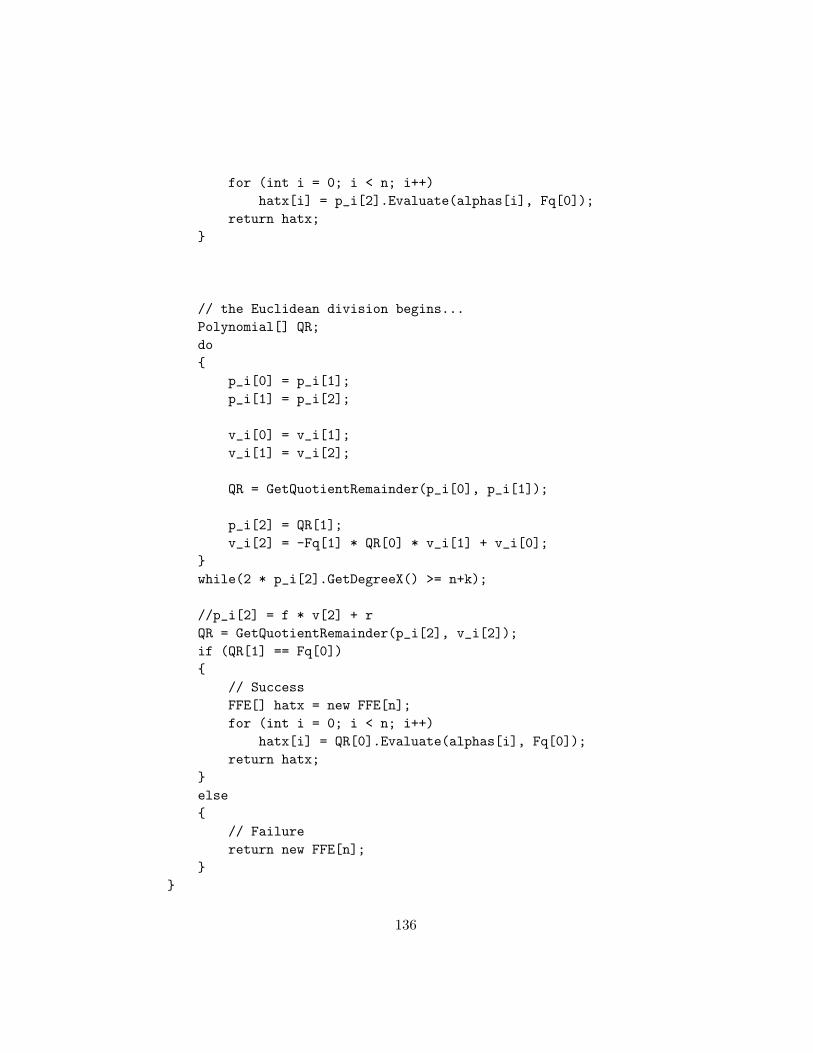
for (int i = 0; i < n; i++)hatx[i] = p_i[2].Evaluate(alphas[i], Fq[0]);

return hatx;

// the Euclidean division begins...Polynomial[] QR;do

p_i[0] = p_i[1];p_i[1] = p_i[2];

v_i[0] = v_i[1];v_i[1] = v_i[2];

QR = GetQuotientRemainder(p_i[0], p_i[1]);

p_i[2] = QR[1];v_i[2] = -Fq[1] * QR[0] * v_i[1] + v_i[0];

while(2 * p_i[2].GetDegreeX() >= n+k);

//p_i[2] = f * v[2] + rQR = GetQuotientRemainder(p_i[2], v_i[2]);if (QR[1] == Fq[0])

// SuccessFFE[] hatx = new FFE[n];for (int i = 0; i < n; i++)

hatx[i] = QR[0].Evaluate(alphas[i], Fq[0]);return hatx;

else

// Failurereturn new FFE[n];

136

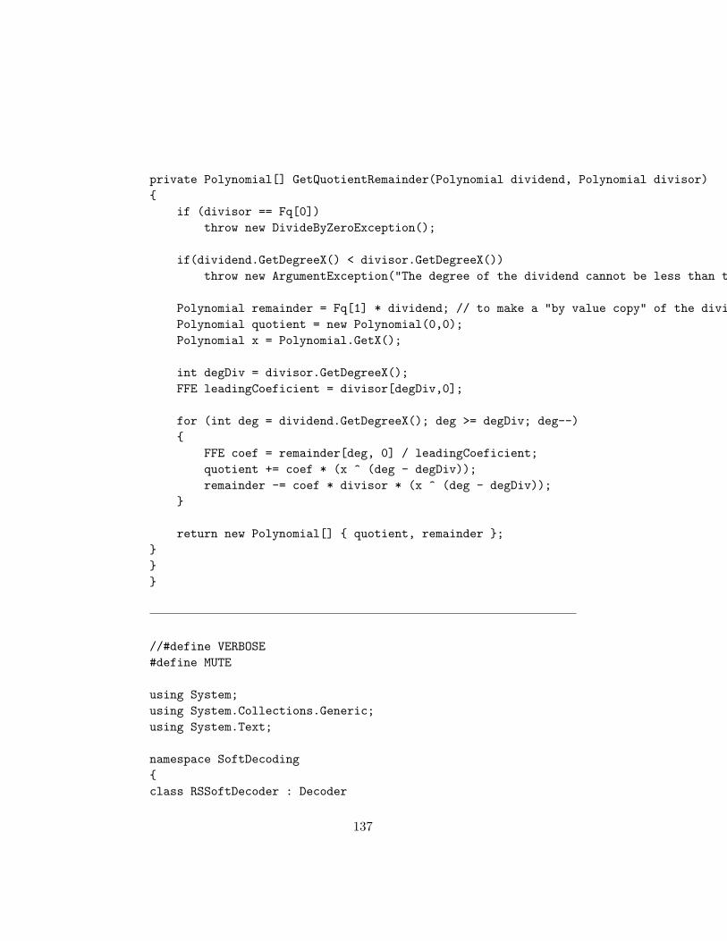
private Polynomial[] GetQuotientRemainder(Polynomial dividend, Polynomial divisor)

if (divisor == Fq[0])throw new DivideByZeroException();

if(dividend.GetDegreeX() < divisor.GetDegreeX())throw new ArgumentException("The degree of the dividend cannot be less than the degree of the divisor.");

Polynomial remainder = Fq[1] * dividend; // to make a "by value copy" of the dividendPolynomial quotient = new Polynomial(0,0);Polynomial x = Polynomial.GetX();

int degDiv = divisor.GetDegreeX();FFE leadingCoeficient = divisor[degDiv,0];

for (int deg = dividend.GetDegreeX(); deg >= degDiv; deg--)

FFE coef = remainder[deg, 0] / leadingCoeficient;quotient += coef * (x ^ (deg - degDiv));remainder -= coef * divisor * (x ^ (deg - degDiv));

return new Polynomial[] quotient, remainder ;

//#define VERBOSE#define MUTE

using System;using System.Collections.Generic;using System.Text;

namespace SoftDecodingclass RSSoftDecoder : Decoder

137

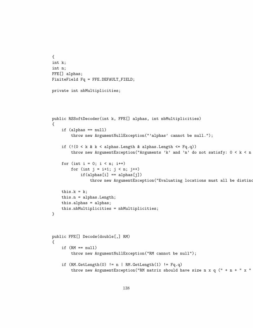
int k;int n;FFE[] alphas;FiniteField Fq = FFE.DEFAULT_FIELD;

private int nbMultiplicities;

public RSSoftDecoder(int k, FFE[] alphas, int nbMultiplicities)

if (alphas == null)throw new ArgumentNullException("’alphas’ cannot be null.");

if (!(0 < k & k < alphas.Length & alphas.Length <= Fq.q))throw new ArgumentException("Arguments ’k’ and ’n’ do not satisfy: 0 < k < n <= q, where ’q’ is the size of the field.");

for (int i = 0; i < n; i++)for (int j = i+1; j < n; j++)

if(alphas[i] == alphas[j])throw new ArgumentException("Evaluating locations must all be distinct");

this.k = k;this.n = alphas.Length;this.alphas = alphas;this.nbMultiplicities = nbMultiplicities;

public FFE[] Decode(double[,] RM)

if (RM == null)throw new ArgumentNullException("RM cannot be null");

if (RM.GetLength(0) != n | RM.GetLength(1) != Fq.q)throw new ArgumentException("RM matrix should have size n x q (" + n + " x " + Fq.q + ").");

138

int[,] M = GreedyMAA(RM);

int omega = ComputeOmega(Cost(M));List<Polynomial> polyList = ListDecode(M, omega);

if (polyList.Count == 0)

//throw new Exception("Decoding failed");return new FFE[n];

double maxProba = 0;Polynomial best = polyList[0];

foreach (Polynomial poly in polyList)

double proba = 1;for (int i = 0; i < n; i++)

for (int j = 0; j < Fq.q; j++)if (poly.Evaluate(alphas[i], Fq[0]) == Fq[j])

proba *= RM[i, j];

if (proba > maxProba)

maxProba = proba;best = poly;

#if !MUTEConsole.WriteLine("\n--== RESULT ==--\n" + best);

#endifFFE[] x = new FFE[n];for (int i = 0; i < n; i++)

x[i] = best.Evaluate(alphas[i], Fq[0]);

return x;

public int[,] GreedyMAA(double[,] RM)

139

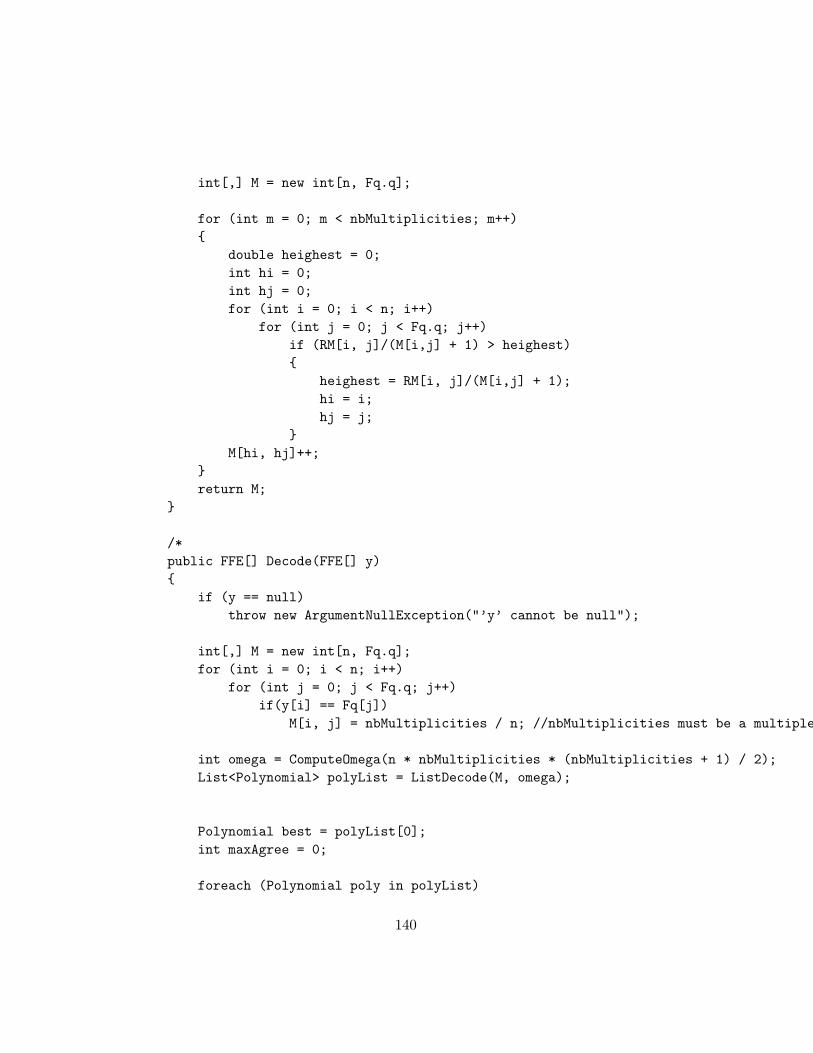
int[,] M = new int[n, Fq.q];

for (int m = 0; m < nbMultiplicities; m++)

double heighest = 0;int hi = 0;int hj = 0;for (int i = 0; i < n; i++)

for (int j = 0; j < Fq.q; j++)if (RM[i, j]/(M[i,j] + 1) > heighest)

heighest = RM[i, j]/(M[i,j] + 1);hi = i;hj = j;

M[hi, hj]++;

return M;

/*public FFE[] Decode(FFE[] y)

if (y == null)throw new ArgumentNullException("’y’ cannot be null");

int[,] M = new int[n, Fq.q];for (int i = 0; i < n; i++)

for (int j = 0; j < Fq.q; j++)if(y[i] == Fq[j])

M[i, j] = nbMultiplicities / n; //nbMultiplicities must be a multiple of n!!!

int omega = ComputeOmega(n * nbMultiplicities * (nbMultiplicities + 1) / 2);List<Polynomial> polyList = ListDecode(M, omega);

Polynomial best = polyList[0];int maxAgree = 0;

foreach (Polynomial poly in polyList)

140

int agree = 0;for (int i = 0; i < n; i++)

if (poly.Evaluate(alphas[i], Fq[0]) == y[i])agree++;

if (agree > maxAgree)

maxAgree = agree;best = poly;

#if !MUTEConsole.WriteLine("\n--== RESULT ==--\n" + best);

#endifFFE[] x = new FFE[n];for (int i = 0; i < n; i++)

x[i] = best.Evaluate(alphas[i], Fq[0]);

return x;*/

public List<Polynomial> ListDecode(int[,] M, int omega)

Polynomial Q = FindQ(M, omega);#if !MUTE

Console.WriteLine("\n--== Interpolation finished ==--\n" + Q+"\n");#endif

List<Polynomial> polyList = new List<Polynomial>();FactorizeRR(Q, 0, new Polynomial(0,0), polyList);

#if !MUTEConsole.WriteLine("\n--== Factorization finished ==--");foreach (Polynomial poly in polyList)

Console.WriteLine(poly);#endif

return polyList;

141

public static long C(int j, int n)

long ans = 1;

if (j > n / 2)j = n-j;

for (int i = 0; i < j; i++)ans *= (n - i);

ans /= Fact(j);

return ans;

static int Fact(int n)

if (n <= 1)return 1;

elsereturn n * Fact(n - 1);

// divides by the greatest power of X possible and shrink the array as much as possiblePolynomial NormalizeX(Polynomial Q)

int xPowerDivisor = -1;

for (int i = 0; i <= Q.GetMaxDegX() & xPowerDivisor == -1; i++)for (int j = 0; j <= Q.GetMaxDegY(); j++)

if (Q[i, j] != Fq[0])

xPowerDivisor = i;break;

if (xPowerDivisor == -1) return new Polynomial(0,0);

142

int xDegreesInExcess = -1;for (int i = Q.GetMaxDegX(); i > 0 & xDegreesInExcess == -1; i--)

for (int j = 0; j <= Q.GetMaxDegY(); j++)if (Q[i, j] != Fq[0])

xDegreesInExcess = Q.GetMaxDegX() - i;break;

if (xPowerDivisor > 0 | xDegreesInExcess > 0)

Polynomial divided = new Polynomial(Q.GetMaxDegX() - xPowerDivisor - xDegreesInExcess, Q.GetMaxDegY());for (int i = 0; i <= divided.GetMaxDegX(); i++)

for (int j = 0; j <= divided.GetMaxDegY(); j++)divided[i, j] = Q[i + xPowerDivisor, j];

return divided;else

return Q;

public Polynomial Y_To_XY_Plus_Gamma(Polynomial Q, FFE gamma)

Polynomial result = new Polynomial(Q.GetMaxDegX() + Q.GetMaxDegY(), Q.GetMaxDegY());

for (int i = 0; i <= Q.GetMaxDegX(); i++)for (int j = 0; j <= Q.GetMaxDegY(); j++)

for (int d = 0; d <= j; d++)result[i + d, d] += Fq[(int) C(d, j) % Fq.p] * Q[i, j] * (gamma ^ (j - d));

return result;

Polynomial HasseDerivative(Polynomial Q, int dx, int dy)

143

if (dx == 0 & dy == 0)return Q;

Polynomial DQ = new Polynomial(Math.Max(Q.GetMaxDegX() - dx,0), Math.Max(Q.GetMaxDegY() - dy,0));for (int i = 0; i <= Q.GetMaxDegX() - dx; i++)

for (int j = 0; j <= Q.GetMaxDegY() - dy; j++)

int ii = i + dx;int jj = j + dy;long ci = C(dx, ii);long cj = C(dy, jj);DQ[i, j] = Fq[(int) (C(dx,ii) % Fq.p)] * Fq[(int) (C(dy,jj) % Fq.p)] * Q[ii, jj];

return DQ;

public int Cost(int[,] M)

int cost = 0;

for (int i = 0; i < M.GetLength(0); i++)for (int j = 0; j < M.GetLength(1); j++)

cost += M[i, j] * (M[i, j] + 1) / 2;

return cost;

public int ComputeOmega(int cost)

// this is a lower bound on Omega(cost)int omega = (int) Math.Sqrt(2 * (k - 1) * cost) - 1;int L = omega / (k - 1);

// now, we find the least Omega such that NbMonoms(Omega) > costint nbMonoms = (L + 1) * (omega+1 - L * (k - 1) / 2);

144

while (nbMonoms <= cost)

omega++;L = omega / (k - 1);nbMonoms = (L + 1) * (omega+1 - L * (k - 1) / 2);

return omega;

public Polynomial FindQ(int[,] M, int omega)

int L = omega / (k - 1);

Polynomial[] Q = new Polynomial[L + 1];int[] wdeg = new int[L + 1];for (int l = 0; l <= L; l++)

Q[l] = new Polynomial(omega, L);Q[l][0, l] = Fq[1];wdeg[l] = l * (k - 1);

FFE[] lambdas = new FFE[L + 1];int lowestL;

for (int i = 0; i < alphas.Length; i++)for (int j = 0; j < Fq.q; j++)if (M[i, j] != 0)

#if VERBOSEConsole.WriteLine("i,j: " + alphas[i] + "," + Fq[j]);

#endif

for (int u = 0; u < M[i, j]; u++)for (int v = 0; v < M[i, j] - u; v++)

#if !MUTE

145

#if !VERBOSEConsole.Write(".");

#endif#endif

lowestL = -1;for (int l = 0; l <= L; l++)

Polynomial Duv = HasseDerivative(Q[l], u, v);lambdas[l] = Duv.Evaluate(alphas[i], Fq[j]);

#if VERBOSEConsole.WriteLine("Q["+l+"](x,y) = " +Q[l] + "\n => D_" + u + "," + v + " = " + Duv + "\n => lambda (" + alphas[i] + "," + Fq[j] + ") = " + lambdas[l]);

#endifif (lambdas[l] != Fq[0])

if (lowestL == -1 || wdeg[l] < wdeg[lowestL])lowestL = l;

#if VERBOSE

Console.WriteLine("\n" + "Lowest l is: " + lowestL + "\n");#endif

if (lowestL != -1)

for (int l = 0; l <= L; l++)if (lambdas[l] != Fq[0] & l != lowestL)

Q[l] = Q[l] - (lambdas[l]/lambdas[lowestL]) * Q[lowestL];

Q[lowestL] = (Polynomial.GetX() - alphas[i]) * Q[lowestL];wdeg[lowestL] += 1;

return Q[ArgMin(wdeg)];

static int ArgMin(int[] array)

int argMin = -1;

146

for (int i = 0; i < array.Length; i++)if (argMin == -1 || array[i] < array[argMin])

argMin = i;

return argMin;

public void FactorizeRR(Polynomial Q, int i, Polynomial f, List<Polynomial> fList)

Q = NormalizeX(Q);

#if VERBOSEConsole.WriteLine("i: " + i + " - k: " + k);

#elif !MUTEConsole.Write(".");

#endif

for (int j = 0; j < Fq.q; j++)

FFE eval = Q.Evaluate(Fq[0], Fq[j]);if(eval == Fq[0])

#if VERBOSE

Console.WriteLine(Q);Console.WriteLine("Q(0," + Fq[j] + ") = " + Q.Evaluate(Fq[0], Fq[j]));

#endifPolynomial otherF = f + Fq[j] * (Polynomial.GetX()^i);

if (i == k - 1)fList.Add(otherF);

else

Polynomial nextQ = Y_To_XY_Plus_Gamma(Q, Fq[j]);FactorizeRR(nextQ, i + 1, otherF, fList);

147

A.4 Channels

using System;using System.Collections.Generic;using System.Text;

namespace SoftDecodingpublic class NoiselessChannel : Channelprotected FiniteField Fq;

public NoiselessChannel(FiniteField Fq)

this.Fq = Fq;

FFE[] received;

public void Send(FFE[] word)

received = word;

public double[,] Receive()

int n = received.Length;double[,] RM = new double[n, Fq.q];for (int i = 0; i < n; i++)

for (int j = 0; j < Fq.q; j++)if (received[i] == Fq[j])

RM[i, j] = 1.0;return RM;

148

public void SetVariance(double variance)

//nothing to do

using System;using System.Collections.Generic;using System.Text;

namespace SoftDecodingclass QarySymetricChannel : Channelpublic readonly FiniteField Fq;public readonly double p_err;

private Random random = new Random();

private FFE[] received;private double[,] RM;

public QarySymetricChannel(FiniteField Fq, double p_err)

this.Fq = Fq;this.p_err = p_err;

public void Send(FFE[] word)

int n = word.Length;received = new FFE[n];for (int i = 0; i < word.Length; i++)

if (random.NextDouble() > p_err)received[i] = word[i];

else

149

doreceived[i] = Fq[random.Next(Fq.q)];

while (received[i] == word[i]);

RM = new double[word.Length, Fq.q];for (int i = 0; i < n; i++)

for (int j = 0; j < Fq.q; j++)if (received[i] == Fq[j])

RM[i, j] = 1.0 - p_err;else

RM[i, j] = p_err / (Fq.q - 1);

public double[,] Receive()

return RM;

using System;using System.Collections.Generic;using System.Text;

namespace SoftDecodingclass ExtendedBinaryChannel : ChannelFiniteField Fq;double p_err;

double[,] RM;FFE[] received;

private Random random = new Random();private int m;

150

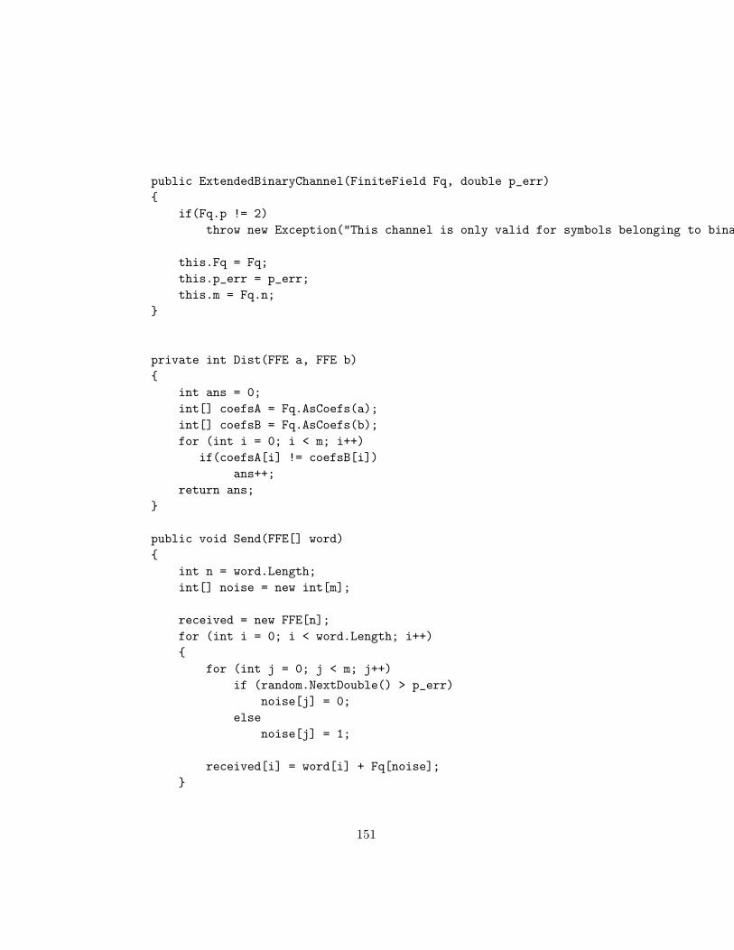
public ExtendedBinaryChannel(FiniteField Fq, double p_err)

if(Fq.p != 2)throw new Exception("This channel is only valid for symbols belonging to binary power fields.");

this.Fq = Fq;this.p_err = p_err;this.m = Fq.n;

private int Dist(FFE a, FFE b)

int ans = 0;int[] coefsA = Fq.AsCoefs(a);int[] coefsB = Fq.AsCoefs(b);for (int i = 0; i < m; i++)

if(coefsA[i] != coefsB[i])ans++;

return ans;

public void Send(FFE[] word)

int n = word.Length;int[] noise = new int[m];

received = new FFE[n];for (int i = 0; i < word.Length; i++)

for (int j = 0; j < m; j++)if (random.NextDouble() > p_err)

noise[j] = 0;else

noise[j] = 1;

received[i] = word[i] + Fq[noise];

151

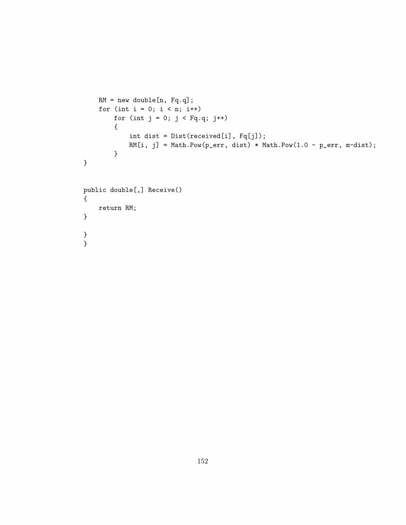
RM = new double[n, Fq.q];for (int i = 0; i < n; i++)

for (int j = 0; j < Fq.q; j++)

int dist = Dist(received[i], Fq[j]);RM[i, j] = Math.Pow(p_err, dist) * Math.Pow(1.0 - p_err, m-dist);

public double[,] Receive()

return RM;

152