Vol.:(0123456789)

SN Applied Sciences (2019) 1:1157 | https://doi.org/10.1007/s42452-019-1201-1

Research Article

Algebraic reconstruction technique combined with Monte Carlo method for weight matrix calculation in gamma ray transmission tomography

Chhavi Agarwal1  · Amol Mhatre1 · Sabyasachi Patra1 · Sanhita Chaudhury1 · A. Goswami2

© Springer Nature Switzerland AG 2019

AbstractIn the present work, the algebraic reconstruction technique (ART) combined with Monte Carlo method has been pro-posed for image reconstruction in gamma ray transmission tomography, which is generally used for the nondestructive assay of special nuclear materials. The Monte Carlo method has been explored to generate the weight matrix, which is required for executing ART algorithm. The method has been successfully demonstrated using a two-dimensional tomo-graphic set-up with circular sample. The advantage of the method is that it is generalized, with no assumptions regard-ing weight matrices and is easily extendable to three dimensional systems, where other classical approaches become cumbersome. Moreover, the method is computationally simple and less time consuming unlike full scale Monte Carlo simulations.

Keywords Nondestructive assay · Transmission tomography · Image reconstruction · ART algorithm · Monte Carlo method

1 Introduction

Passive nondestructive assay (NDA) techniques are widely used for the assay of special nuclear materials (SNMs) such as uranium and plutonium at different stages of nuclear fuel cycle [1]. One of the most important applications of gamma ray based NDA technique is the assay of low-density 200 L waste drums containing low/intermediate level of activity. Segmented gamma ray assay (SGA) is the most commonly employed technique for the assay of such heterogeneous samples [2–7]. In this technique, the radial inhomogeneity of the waste drum is averaged out by rotating the drum during counting. Similarly the drum is counted in successive segments to take care of the vertical inhomogeneity. This technique accounts for variation of matrix materials in different segments, it assumes both the source and the matrix to be homogeneously distributed in each segment. For situations where the radionuclide

source distribution as well as matrix distribution is signifi-cantly heterogeneous, SGA technique may lead to large errors [8]. Also, the heterogeneity will lead to difficulty in preparing representative standards. Another advanced NDA technique to assay radioactive waste is tomographic gamma scanning (TGS) which combines high resolution gamma spectrometry with low spatial resolution three-dimensional emission and transmission image reconstruc-tion techniques to yield a coarse 3-dimensional image of the radionuclide and matrix density distributions, with a typical spatial resolution of 6 cm [8–16]. This technique is capable of providing quantitative results with bet-ter accuracy where the radionuclide is distributed non-uniformly in a heterogeneous matrix. The basic principle of a TGS assay is similar to X-ray tomography, which is widely used in not only medical imaging but also finds its applications in different industries [17, 18]. While the X-ray based tomography facilitates faster scans due to

Received: 6 May 2019 / Accepted: 30 August 2019 / Published online: 4 September 2019

* Chhavi Agarwal, cagarwal@barc.gov.in | 1Radiochemistry Division, Bhabha Atomic Research Centre, Mumbai 400085, India. 2Formerly, Radiochemistry Division, Bhabha Atomic Research Centre, Mumbai 400085, India.

Vol:.(1234567890)

Research Article SN Applied Sciences (2019) 1:1157 | https://doi.org/10.1007/s42452-019-1201-1

the high intensity of X-ray sources, the gamma ray based tomography supersedes owing to the high penetration of gamma rays, portable installation and less cost. Apart from nondestructive assay of nuclear waste, over the last decade, the gamma ray based tomographic technique has been increasingly used for diverse applications such as multiphase flow analysis or process tomography [19], in evaluation of soil structure [20] and in chemical reactor engineering studies [21]. The technique also finds appli-cation in radiography [22], metrology [23] and in inspec-tion of distillation towers [24]. Gamma ray tomographic technique has been used to locate solid deposits in vessel by measuring the transmission of monoenergetic gamma rays from a 137Cs source [25]. The gas–liquid phase distri-bution in commercially available industrial pumps using gamma ray tomography is also extensively studied [26, 27]. Recently, the gamma scanning has been coupled with gamma based tomography to inspect a broken pipe struc-ture inside a laboratory scale vessel [28].

In a TGS assay, the sample is viewed as a composite of small volumes, called as voxels. For a two-dimensional set-up, the term ‘voxel’ is generally replaced with ‘pixel’. Both the radioactivity and matrix distributions in the sample are obtained by measuring the emission and transmis-sion spectra respectively at all the possible translations and rotations of sample. Each measurement is called as projection. Each projection (pi) is the single ray consisting of the sum of all the voxels/pixels in that ray (fj), given by:

where M is the total number of projections, N is the total number of voxels and wij is the weight factor that repre-sents the contribution of the jth voxel to the ith ray sum. These projections are then used in image reconstruction algorithms to develop three-dimensional maps of the source distribution and matrix attenuation within the sample. Generally, the image reconstruction of each voxel is complex, since the voxels that lie between the source and the detector vary as the drum rotates and translates. Nevertheless, by careful geometric definition of the fixed and rotating coordinate systems and the application of efficient reconstruction algorithms, high throughput, low bias, and adequate image reconstruction can be achieved.

Two types of methods are used for reconstruction of image in tomography, (i) analytical methods such as back projection method [29] involving radon transform and (ii) iterative methods such as algebraic reconstruc-tion technique (ART), multiplicative algebraic recon-struction technique (MART) etc. Generally, the back pro-jection methods are commercially used, though iterative

(1)N∑

j=1

wijfj = pi i = 1, 2,… ,M

techniques give better images. In the latter technique, correction to the image of the sample is applied at each iteration. This procedure is repeated until a satisfactory accuracy is achieved. The commercial success of this technique is limited by the long computational time. Compared to other statistical iterative algorithms such as Maximum Likelihood Expectation–Maximization (MLEM) [30], the algebraic reconstruction technique (ART) [31, 32] has a higher convergence rate. The ART was pro-posed by Ref. [32] and begins with some initial estimate of the activity/linear attenuation coefficient (image) at each pixel to be reconstructed (usually as a uniformly gray image). The estimated projection in the subsequent steps is obtained by summing the contribution of pix-els along that projection and is thrown back across the reconstruction matrix from which it came. The discrep-ancy between the measured (pi) and the corresponding estimated projection (qi) is used to assign a new estimate of ‘f’, as given by:

where f(i − 1, j) and f (i, j) represents the estimate of activ-ity/linear attenuation coefficient in the jth pixel at (i − 1)th and ith projection respectively for emission/transmis-sion measurement respectively. ART modifies this estimate repeatedly until the pixel values appear to converge. A suitable criterion for convergence is used to get the activ-ity/linear attenuation coefficient in each pixel. Weight matrix is an indispensable element in algebraic image reconstruction techniques in computed tomography. Due to the finite detector size and beam width, varying fractions of the pixels are seen by the beam/detector in different projections. Also, the shape of the pixels seen changes from rectangular through trapezoid to triangu-lar depending on the angle of a projection. Therefore, the contribution of a pixel to the weight matrix varies with projection [30]. Classical analytical approaches to weight matrix generation include a line length and a strip-area model [33–35]. In the line length model, the weight matrix is the beam intersection length in the pixel and in the strip area model, it is the intersection area divided by the beam width. Along with these two, other analytical approaches are also available in literature [36]. In all these approaches, the required parameters such as intersection length, area or the beam width are obtained by analytical modeling. However, this becomes difficult and cumbersome for 3-dimensional image reconstructions. Also, due to the var-ying field of view with distances from detector, the weight matrix is not easy to generate. The analytical derivation becomes still more challenging for nonconventional

(2)f (i, j) = f (i − 1, j) +(pi − qi)∑N

k=1w2

ik

wij

Vol.:(0123456789)

SN Applied Sciences (2019) 1:1157 | https://doi.org/10.1007/s42452-019-1201-1 Research Article

system geometries. In order to make the calculations less cumbersome, pixels are replaced by the centroids and the edge and partial volume effects are neglected [31]. Full scale Monte Carlo simulation is another method to generate weight matrix for the required sample-detector system [37–39]. This is particularly useful for 3-dimensional or nonconventional systems where analytical methods become difficult to derive. In fact, the Monte Carlo simu-lations are also used in tomographic imaging to produce large number of datasets from arbitrary source and matrix distributions, generally required for validation of any reconstruction algorithm [37–39]. In this application, as the exact source, matrix and detector characteristics are known; the link between the reconstructed and the actual images can be thoroughly studied. There are several gen-eral purpose codes like Geant4 [40], MCNP [41], Penelope [42] etc. as well as dedicated toolkits such as GATE [38, 43], GAMOS [44] etc. available for this purpose. Mosorov et al. [45] used MCNP5 code to model a gamma ray indus-trial tomography set-up and compared its results with the experimental observations. However, the major problem of Monte Carlo simulations is the long computation times, generally required for achieving reasonable accuracy in simulation of any realistic configurations.

In this work, an ART algorithm combined with Monte Carlo method is presented for image reconstruction in transmission gamma ray tomography. The Monte Carlo method has been proposed for the generation of weight matrix. The advantage of the method is that like full scale Monte Carlo simulation, it can be easily applied to any nonconventional system geometry [38] and takes care of the varying field of view of the sample with respect to detector as a function of rotation and translation. Also, the method is easier to comprehend for three-dimensional image reconstructions [38]. The advantage over full scale Monte Carlo simulations is that the method is computa-tionally less time taking (< 1 min). The method is simple and does not require detailed detector geometry. Also, the method is combined with the reconstruction algorithm at a common platform, unlike the Monte Carlo simulations, where the weight matrix generated needs to be subjected to reconstruction algorithm separately. The applicability of the method has been validated by reconstruction of image from the experimental projection data collected with a simple circular two-dimensional tomography set-up. Transmission experiments through attenuators of dif-ferent materials, placed at different positions in the set-up have been carried out using a collimated beam of 137Cs source. Measurements have been carried out for all the translations and rotations. A FORTRAN program has been written to geometrically scan the sample translationally and rotationally. The experimentally measured projec-tions have been used as inputs in the program. Algebraic

reconstruction technique (ART) has been used to recon-struct the transmission image. Monte Carlo method has been used for calculating the contributions of each pixel to a particular projection. The results of the matrix dis-tributions and linear attenuation coefficients have been presented.

2 Theoretical method

In the present study, the circular sample of diameter Nδ has been superposed on an N x N square matrix, with total of N2 pixels (each of δ × δ cm2 size) as shown in Fig. 1. Geometrical representation of the circular sample with collimated detector and transmission source is shown in Fig. 2. As seen from the figure, the collimated detec-tor and source are placed diametrically opposite to each other in touching configuration with the circular sample. In the present method, instead of rotating the sample, the collimated detector and the transmission source are translationally and rotationally moved. For rotation of the source-detector system by an angle θ, the points A and B are rotated to points C and I respectively (Fig. 2). The co-ordinates of the latter points are given as:

where (x, y) and (x′, y′) are the co-ordinates of point A and B respectively.

(3)

(

x1�

y1�

)

=

(

cos � − sin �

sin � cos �

)

(

x

y

)

(4)

(

x2�

y2�

)

=

(

cos � − sin �

sin � cos �

)

(

x�

y�

)

(x1, y1) (x2, y1)

(x1, y2) (x2, y2)

(a, b)X

(a, b)Yxl xr

Detector collimator

Transmission source collimator

145

62

138

Detector

Fig. 1 Superposition of the circular sample on a square matrix. Inset shows enlarged view of a single pixel and co-ordinates of dif-ferent points are explained in the text

Vol:.(1234567890)

Research Article SN Applied Sciences (2019) 1:1157 | https://doi.org/10.1007/s42452-019-1201-1

The upper limits of the co-ordinates of the lines along which the detector and its collimator need to be translated to scan the full diameter of the sample i.e. points D, H, E and G are obtained by solving the following equations:

Similarly, x2d and y2d is obtained by replacing x1θ by x2θ and y1θ by y2θ. Equations 7 and 8 are solved to get (x3d, y3d):

Similarly, x4d and y4d is obtained by replacing x1θ by x2θ and y1θ by y2θ in Eqs. 7 and 8. Transmission source collimator co-ordinates (x5d, y5d) and (x6d, y6d) are also obtained in a similar way by replacing detector collimator length l with transmission source collimator length, l’ in Eqs. 7 and 8. For each translation, the co-ordinates of the detector collima-tor (i.e. (u1,v1), (u2, v2), (u3, v3) and (u4, v4)) as shown in the inset of Fig. 2, are obtained as:

(5)cos 90◦ =x1�(x1� − x1d) + y1�(y1� − y1d)

(N�∕2)2

(6)x21d

+ y21d

= 2(N�∕2)2

(7)cos 90◦ =x1�(x1� − x3d) + y1�(y1� − y3d)

(N�∕2)(N�∕2 + l)

(8)x23d

+ y23d

= (N�∕2)2 + (N�∕2 + l)2

(9)u1 =(� − rc)x2d + ((N − 1)� + rc)x1d

N�

(10)v1 =(� − rc)y2d + ((N − 1)� + rc)y1d

N�

(11)u2 =(� + rc)x2d + ((N − 1)� − rc)x1d

N�

where rc is the radius of the collimator in front of detector. Also, (u3,v3) and (u4,v4) are obtained from Eqs. (9 and 10) and (11 and 12) respectively, by replacing (x1d, y1d) by (x3d, y3d) and (x2d, y2d) by (x4d, y4d) respectively. The transmission source co-ordinates are then obtained as:

Once the scan range of detector and transmission source collimator is calculated, translational movement of the two is achieved analytically by incrementing their position by δ, the pixel length. The detector-source system is rotated at intervals of 22.5° and for each rotation, the sample is scanned translationally by placing the detector and the source at the centre of the left most column of the sample matrix (i.e. at a distance of δ/2) to the centre of the right most column (i.e. at a distance of (Nδ − δ/2)). This makes the total number of projections to 16N (16 rotations × N translations). The experimental count rate data constitute the projections which are given as an input in the program.

The image reconstruction by ART algorithm also requires weight matrix as an input, which represents the contribution of each pixel in a projection. As seen from Fig. 1, each pixel will contribute differently in different projections and this will depend on the fraction of the pixel covered by the passage of the transmission source

(12)v2 =(� + rc)y2d + ((N − 1)� − rc)y1d

N�

(13)u5 =�x6d + (N − 1)�x5d

N�

(14)v5 =�y6d + (N − 1)�y5d

N�

Fig. 2 Geometrical represen-tation of the circular sample with collimated detector and transmission source. The co-ordinates are explained in the text

Nδ

A B

D

H

FC

I

(0,0)

O

(-Nδ/2,0)

(x1θ, y1θ)

(x2θ, y2θ)

(x1d, y1d)

(x2d, y2d)

(xd, yd)

Nδ/2

dθ

θ

Collimator

NaI(Tl) detector

Transmission source

Collimator θ

(x3d, y3d)

(x4d, y4d)

(u5, v5)

(x5d, y5d)

(x6d, y6d)

(u3, v3)

(u4, v4)(u1, v1)

(u2, v2)

Detector collimator

l

l’

E

G

K

LM

J

Vol.:(0123456789)

SN Applied Sciences (2019) 1:1157 | https://doi.org/10.1007/s42452-019-1201-1 Research Article

gamma rays reaching the detector. In the present work, the weight matrix is obtained using Monte Carlo method. In this method, random points (a, b) are generated in a pixel bound by the coordinates (x1, y1), (x2, y1), (x1, y2) and (x2, y2) respectively as shown in the inset of Fig. 1. The point is accepted if the condition (a2+ b2) ≤ rs

2 is satisfied which ensures that the point also lies within the sample of radius rs. Out of all the random points (a, b) lying within the sample and the pixel, only a fraction of points may lie in the path of the beam defined by the collimated trans-mission source. For example as shown in the inset of Fig. 1, while both points X and Y lie within the sample and the pixel, point X lies outside the path of the beam but point Y lie inside it. Therefore, only point Y will contribute to the attenuation of the gamma rays emitted by the transmis-sion source. To check geometrically whether the randomly chosen points lie inside the beam path or not, the limits of the beam path along x-axis corresponding to the y-co-ordinate of the random point i.e. ‘b’, is obtained as:

All the random points (a, b) for which the x-co-ordinate, ‘a’ lies within xl and xr are considered as the points contribut-ing to the attenuation of the gamma rays originating from the transmission source. In this way, a large number of ran-dom points are generated within the pixel and checked for their contribution in the projection. The contribution of a pixel in a particular projection i.e. wij is given by:

where, n represents the number of random points which are within the pixel as well as in the beam path within the pixel and No is the total number of random points lying within the pixel in the sample. This fractional contribution from each pixel is then multiplied with the pixel length (δ) to get the fractional length covered by the gamma rays in the pixel. The estimated projection, qi is then obtained as:

where µij represents the estimated linear attenuation coef-ficient in jth pixel for ith projection. In this way, all the 16 N projections are sequentially considered to update the val-ues of linear attenuation coefficients (µij) in different pixels using ART algorithm (Eq. 2). The full set of 16N projections is considered as a single iteration. In this way, the process

(15)xl =(b − v5) × (u3 − u5)

(v3 − v5)+ u5

(16)xr =(b − v5) × (u4 − u5)

(v4 − v5)+ u5

(17)wij =n

No

(18)qi =

N∑

j=1

wij�ij

of modifying the image using ART algorithm is iteratively repeated until the discrepancy (Δpq) as given by Eq. 19, reaches a minimum:

3 Experimental

The prototype TGS system used in the measurements consisted of a circular perspex plate of 43.18 cm diameter with concentric grooves at a distance of 2 cm to place the attenuator sample. The arrangement of the prototype sys-tem is shown schematically in Fig. 3. Attenuators of differ-ent matrices (aluminium, lead and steel) were placed at well defined positions in the perspex plate as attenuating matrices. The transmittance through these samples was measured using a collimated beam of 137Cs as the trans-mission source using a well collimated NaI(Tl) detector placed diametrically opposite to the transmission source. Attenuators of two different lengths (2.54 and 5.08 cm) and ~ 0.5 cm or 1 cm thickness (depth) were used. The height of the attenuators was taken to be sufficient to fully obstruct the transmission source gamma ray path. Table 1 gives the details of the attenuators used. The count rate of the transmitted ray at different translations and rota-tions of the circular sample was measured (I) for a fixed attenuator position by accumulating the counts for 150 s. The rotation of the sample was realized by moving the whole perspex plate systematically at intervals of 22.5°. The translation along the X-axis (Fig. 1) was done by mov-ing perspex plate in 2.54 cm intervals. For each rotation, the sample was scanned translationally by moving the detector from the centre of the left most column of the sample matrix to the centre of the right most column. This makes the total number of projections to 272. The count rate of the transmission ray in the absence of the attenu-ator sample was also measured to give the unattenuated count rate (Io).

(19)Δpq =

√

√

√

√1

M

M∑

i=1

(pi − qi)2

A�enua�ng blockTransmission source

Fig. 3 A prototype two dimensional transmission tomography sys-tem

Vol:.(1234567890)

Research Article SN Applied Sciences (2019) 1:1157 | https://doi.org/10.1007/s42452-019-1201-1

4 Results and discussion

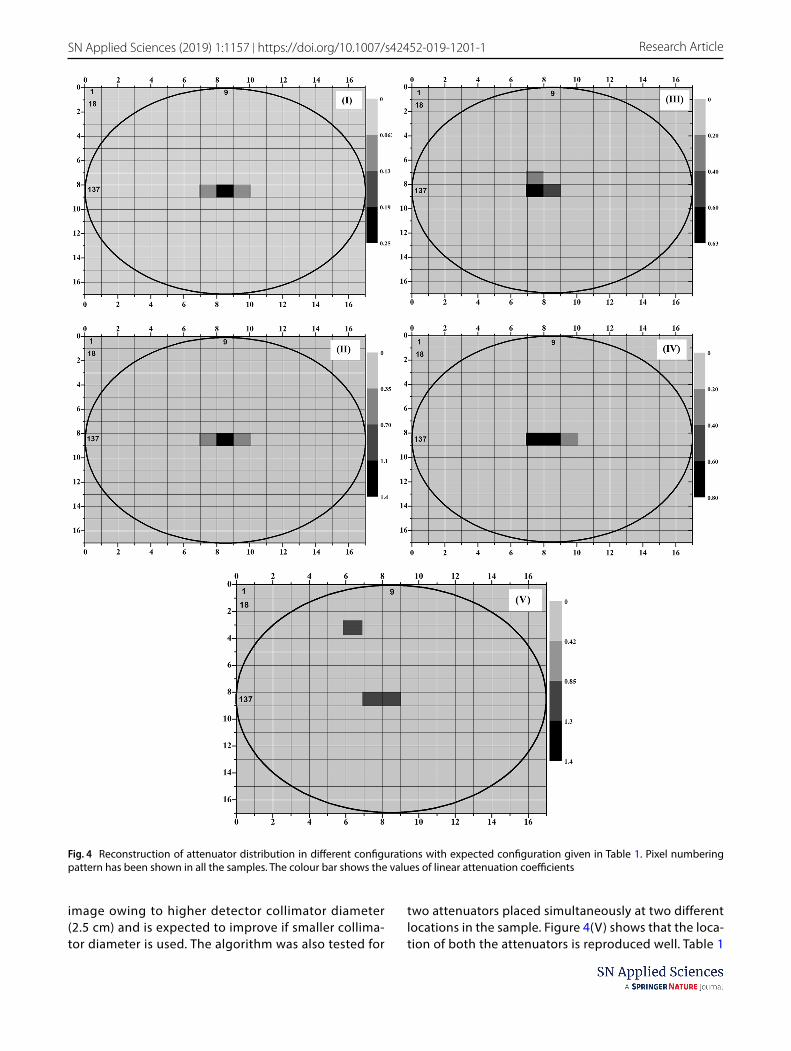
In the present study, a FORTRAN program has been written to geometrically scan the sample translation-ally and rotationally as explained in the theoretical sec-tion. The circular sample of 43.18 cm diameter has been superposed on a 17 × 17 square matrix, with a total of 289 pixels (each of 2.54 × 2.54 cm2 size). The logarithmic of the transmission of the sample (ln(Io/I)) for different translations and rotations has been given as an input to the FORTRAN program. The detector and transmis-sion source collimator diameter and lengths have been also given as inputs in the program (Table 2). The con-tribution of a pixel in a particular projection i.e. wij has been obtained using Monte Carlo method, as described in the theoretical section. In each pixel, 500 random points have been generated to get its weight fraction, which has been corrected with the pixel length (2.54 cm) to get the fractional length covered by the transmit-ted gamma ray in that pixel. The calculation was done in a desktop personal computer and the time taken for computation was less than a minute. The expected projection data (qi) at each stage of iteration has been obtained using the wij and the estimated values of the

linear attenuation coefficient (Eq. 18). The initial values of the latter have been chosen to be all zero’s, i.e. µ(i, j)= 0 (grey image) and have been updated in each projection using ART algorithm (Eq. 2). Calculation of one full set of 272 projections is considered as a single iteration. After two–three iterations, a minima in the discrepancy (Δpq) has been observed and therefore the calculations have been terminated. Attempt was made to keep number of iterations minimum since ART algorithm is known to accumulate reconstruction errors more significantly with iteration [46]. Figure 4(I–V) shows the reconstructed matrix density image for all the samples, in sequence corresponding to Table 1. It can be seen from the figure, that the spatial location of the attenuators have been well reproduced. Slight diffusiveness to the nearby pixels have been observed, owing to the wide collimator used in the present study. Since in the present study, the num-ber of projections (272) are much less than the number of pixels (289), the data used for reconstruction is under-determined and the solution is not unique. The image may be further improved by increasing the number of projections, which can be achieved using mechanical movement of the sample using motors. The effect of matrix density is clearly seen from the different degree of greyness in the Fig. 4(I-III), for different attenuators i.e. aluminium, lead and steel. The shape of the attenuat-ing material image is different in Fig. 4(III) as compared to the previous two images i.e. Figure 4(I and II). This reflects the difference in length of the two attenuators, with the longer attenuator (length = 5.08 cm) encom-passing two pixels in Fig. 4(III) and the shorter attenu-ator (length = 2.54  cm) encompassing only one pixel in Fig. 4(II). This is clearly visible from the two images. Not much difference in the image is obtained when the attenuator is shifted by one pixel (Fig. 4(IV)) relative to Fig. 4(III). This is also due to the lower resolution of the

Table 1 Attenuator configuration in the sample and expected and obtained linear attenuation coefficients in different samples

Sample no. Attenuator configuration and dimension Expected linear attenua-tion coefficient (cm−1)

Obtained linear attenuation coef-ficient (cm−1) at specified position

Ratio (expected/obtained)

I Al (2.54 cm length and 0.5 cm thickness) at centre (145) 0.25 Pixel 145 0.25 1.00II Lead (2.54 cm length and 0.5 cm thickness) at centre (145) 1.26 Pixel 145 1.41 0.89III Steel (5.08 cm length and 0.5 cm thickness) at centre (145) 0.69 Pixel 145 0.63 1.09

0.69 Pixel 146 0.60 1.14IV Steel (5.08 cm length and 0.5 cm thickness) at 144 0.69 Pixel 144 0.64 1.07

0.69 Pixel 145 0.62 1.10V Pb (5.08 cm length and 0.5 cm thickness) at 144 & Pb

(2.54 cm length and 0.5 cm thickness) at 581.26 Pixel 144 1.10 1.14

1.26 Pixel 145 1.22 1.031.26 Pixel 58 1.27 0.99

Table 2 Parameters given as input in FORTRAN program

Parameters

Detector collimator Length (cm) 10.16 Diameter (cm) 2.5

Transmission source collimator Length (cm) 3.0 Diameter (cm) 1.2

Vol.:(0123456789)

SN Applied Sciences (2019) 1:1157 | https://doi.org/10.1007/s42452-019-1201-1 Research Article

image owing to higher detector collimator diameter (2.5 cm) and is expected to improve if smaller collima-tor diameter is used. The algorithm was also tested for

two attenuators placed simultaneously at two different locations in the sample. Figure 4(V) shows that the loca-tion of both the attenuators is reproduced well. Table 1

Fig. 4 Reconstruction of attenuator distribution in different configurations with expected configuration given in Table 1. Pixel numbering pattern has been shown in all the samples. The colour bar shows the values of linear attenuation coefficients

Vol:.(1234567890)

Research Article SN Applied Sciences (2019) 1:1157 | https://doi.org/10.1007/s42452-019-1201-1

gives the expected and the obtained linear attenuation coefficient values after image reconstruction. It can be seen that in all the cases, the expected and the obtained linear attenuation coefficients have been found to be within 10–13%, showing the efficacy of the analysis.

5 Conclusion

The study proposes a Monte Carlo based method for gen-eration of appropriate weight matrix which is central to using the algebraic reconstruction technique for image reconstruction in gamma ray transmission tomography. The method has been successfully tested for different attenuating matrices such as aluminium, steel and lead, of varying dimensions, placed at different well defined positions in the sample. The method facilitates a faster convergence and the calculations take less than a minute in a normal desktop personal computer. The advantage of the method is that it is easier to implement for noncon-ventional system geometries and three dimensional image reconstructions, where classical approaches become cum-bersome. Also, it easily takes care of the different shapes of the pixels seen by the beam and the detector. Though the studies emphasises on the image reconstruction required for the assay of waste nuclear material in a tomographic gamma assay system, the Monte Carlo based method pro-posed for generation of weight matrix is general and can be applied to any of the diverse application of transmis-sion based tomographic system such as process tomog-raphy, radiography, metrology and in chemical reactor engineering studies.

Funding This research did not receive any specific grant from fund-ing agencies in the public, commercial, or not-for-profit sectors.

Compliance with ethical standards

Conflict of interest The authors declare that they have no conflict of interest.

Ethical approval The authors state that the research was conducted according to ethical standards.

References

1. Reilly D, Ensslin N Jr, Smith H, Kreiner S (1991) Passive nonde-structive assay of nuclear materials. Los Alamos National Labora-tory, New Mexico

2. Martin ER, Jones DF, Parker JL (1977) Gamma-ray measurements with the segmented gamma scan. Los Alamos National Labora-tory report, LA-7059-M

3. Sprinkle JK Jr, T-Hsue S (1987) Recent advances in segmented gamma scanner analysis. Los Alamos National Laboratory report, LA-UR-87-3954

4. Bjork CW (1987) Current segmented gamma scanner technol-ogy. In: Proceedings of 3rd international conference on facility operation safeguards interface, San Diego, CA

5. Cesana A, Terrani M, Sandrelli G (1993) Gamma activity deter-mination in waste drums from nuclear plants. Appl Radiat Isot 44:517–520

6. Filβ P (1995) Relation between the activity of a high-density waste drum and its gamma count rate measured with an unshielded Ge-detector. Appl Radiat Isot 46:805–812

7. Bai YF, MauerhoferE Wang DZ, Odoj R (2009) An improved method for the non-destructive characterization of radioac-tive waste by gamma scanning. Appl Radiat Isot 67:1897–1903

8. Hansen JS (2007) Tomographic gamma ray scanning of ura-nium and plutonium. LA-UR-07-5150, Chapter 4

9. Estep RJ, Prettyman T, Sheppard G (1993) Tomographic Gamma Scanning to measure inhomogeneous nuclear mate-rial matrices from future fuel cycles. LA-UR-93-1637

10. Venkataraman R, Villani M, Croft S, McClay P, McElroy R, Kane S, MuellerW Estep R (2007) An integrated Tomographic Gamma Scanning system for non-destructive assay of radioactive waste. Nucl Instrum Methods Phys Res A 579:375–379

11. Kawasaki S, KondoM Izumi S, Kikuchi M (1990) Radioactivity measurement of drum package waste by a computed tomog-raphy technique. Appl Radiat Isot 41:983–987

12. Estep RJ, Prettyman TH, Sheppard GA (1994) Tomographic gamma scanning to assay heterogeneous radioactive waste. Nucl Sci Eng 118:145–152

13. Venkataraman R, Croft S, Villani M (2005) The next generation in tomographic gamma scanner. In: Annual Symposium on Safeguards and Nuclear Material Management, London, UK

14. Venkataraman R, Villani M, Croft S (2007) An integrated Tomo-graphic γ Scanning system for non-destructive assay of radio-active waste. Nucl Instrum Methods Phys Res A 579:375–379

15. Camp DC, Martz HE, Roberson GP, Decman DJ, Bernardi RT (2002) Nondestructive waste-drum assay for transuranic con-tent bygamma-ray active and passive computed tomography. Nucl Instrum Methods Phys Res A 495:69–83

16. Roy T, More MR, Ratheesh J, Sinha A (2017) Active and pas-sive CT for waste assay using LaBr 3(Ce) detector. Radiat Phys Chem 130:29–34

17. Hamideen MS, Sharaf J, Al-Saleh KA, Shaderma M (2011) Description of a transmission X-ray computed tomography scanner. Radiat Phys Chem 80:1162–1165

18. Luggar RD, Morton EJ, Jenneson PM, Key MJ (2001) X-ray tomographic imaging in industrial process control. Radiat Phys Chem 61:785–787

19. Bieberle A, Nehring H, Berger R, Arlit M, Härting HU, Schubert M, Hampel U (2013) Compact high-resolution gamma-ray computed tomography system for multiphase flow studies. Rev Sci Instrum 84:1–10

20. Pires LF, Borges JA, Bacchi OO, Reichardt K (2010) Twenty-five years of computed tomography in soil physics: a lit-erature review of the Brazilian contribution. Soil Tillage Res 110:197–210

21. Boyer C, Fanget B (2002) Measurement of liquid flow distribution in trickle bed reactor of large diameter with a new gamma-ray tomographic system. Chem Eng Sci 57:1079–1089

22. Adams R, Zboray R (2017) Gamma radiography and tomog-raphy with a CCD camera and Co-60 source. Appl Radiat Isot 127:22–26

23. Kruth J, Bartscher M, Carmignato S, Schmitt R, Chiffre LD, Weck-enmann A (2011) Computed tomography for dimensional metrology. CIRP Ann Manuf Technol 60(2):821–842

Vol.:(0123456789)

SN Applied Sciences (2019) 1:1157 | https://doi.org/10.1007/s42452-019-1201-1 Research Article

24. Haraguchia MI, Calvo WAP, Kim HY (2018) Tomographic 2-D gamma scanning for industrial process troubleshooting. Flow Meas Instrum 62:235–245

25. Cattle BA, Fellerman AS, West RM (2004) On the detection of solid deposits using gamma ray emission tomography with lim-ited data. Meas Sci Technol 15:1429–1439

26. Bieberle A, Schäfer T, Neumann M, Hampel U (2015) Validation of high-resolution gamma-ray computed tomography for quan-titative gas holdup measurements in centrifugal pumps. Meas Sci Technol 26:095304–095316

27. Sultan AJ, Sabri LS, Al-Dahhan MH (2018) Impact of heat-exchanging tube configurations on the gas holdup distribution in bubble columns using gamma-ray computed tomography. Int J Multiph Flow 106:202–219

28. Saengchantr D, Srisatit S, Chankow N (2019) Development of gamma ray scanning coupled with computedtomographic tech-nique to inspect a broken pipe structure insidelaboratory scale vessel. Nucl Eng Technol 51:800–806

29. Kumar U, Ramakrishna GS, Datta SS, Ravindran VR (2000) Pro-totype gamma ray computed tomographic imaging system for industrial applications. Insight 42:662–666

30. Shepp A, Vardi Y (1982) Maximum likelihood reconstruction for emission tomography. IEEE Trans Med Imaging MI-I:113–122

31. Gordon R (1974) A tutorial on Algebraic Reconstruction Tech-niques (ART). IEEE Trans NS-2121:78–93

32. Gordon R, Bender R, Herman GT (1970) Algebraic Reconstruction Techniques (ART) for three-dimensional electron microscopy and X-ray photography. J Theor Biol 29:477–481

33. Fessler J (2008) Iterative methods for image reconstruction. ISBI Tutorial

34. Khorsandi M, Feghhi SAH (2015) Development of image recon-struction for Gamma-ray CT of large-dimension industrial plants using Monte Carlo simulation. Nucl Instrum Methods Phys Res A B356–357:176–185

35. Askari M, Ali Taheri, Larijani MM, Movafeghi A (2019) Industrial gamma computed tomography using high aspect ratio scintil-lator detectors (A Geant4 simulation). Nucl Instrum Methods Phys Res A 923:109–117

36. Industrial Process Gamma Tomography, International Atomic Energy Agency, Vienna, Austria, IAEA-Tecdoc-1589, May 2008, 21 p

37. Gillam JE, Rafecas M (2016) Monte Carlo simulations and image reconstruction for novel imaging scenarios in emission tomog-raphy. Nucl Instrum Methods Phys Res A 809:76–88

38. Buvat I, Lazaro D (2006) Monte Carlo simulations in emission tomography and GATE: an overview. Nucl Instrum Methods Phys Res A 569:323–329

39. Rogers DWO (2006) Fifty years of Monte Carlo simulations for medical physics. Phys Med Biol 51:R287–R301

40. Agostinelli S, Allison J, Amako K, Apostolakis J et  al (2003) GEANT4—a simulation toolkit. Nucl Instrum Methods Phys Res A 506:250–303

41. Briesmeister JF (1986) MCNP, a general Monte Carlo code for neutron and photon transport. Los Alomos National Laboratory Publication LA 7396-M

42. Salvat F, Fernandez-Varea J, Sempau J (2009) Penelope-2008: a code system for Monte Carlo simulation of electron and photon transport. Technical Report 6416

43. Jan S, Santin G, Struhl D et al (2004) GATE: a simulation toolkit for PET and SPECT. Phys Med Biol 49:4543–4561

44. Arce P, Rato P, Canadas M, Lagares J (2008) Gamos: a Geant4-based easy and flexible framework for nuclear medicine applica-tions. In: Nuclear Science Symposium Conference Record. IEEE, pp 3162–3168

45. Mosorov V, Johansen GA, Maad R, Sankowski D (2011) Monte Carlo simulation for multi-channel gamma-ray process tomog-raphy. Meas Sci Technol 22:055502–055512

46. Mazur EJ, Gordon R (1995) Interpolative algebraic reconstruc-tion techniques without beam partitioning for computed tomography. Med Biol Eng Comput 33:82–86

Publisher’s Note Springer Nature remains neutral with regard to jurisdictional claims in published maps and institutional affiliations.