Algebraic Methods in Mechanism Analysis andSynthesis

Manfred L. Husty

University Innsbruck, Institute of Basic Sciences in Engineering,Technikerstraße 13, A6020 Innsbruck, Austria

email:manfred.husty@uibk.ac.at

Abstract: Algebraic methods in connection with classical multidimensional geometryhave proven to be very efficient in the computation of direct and inverse kinematics ofmechanisms as well as the explanation of strange, pathological behavior. In this paper wegive an overview of the results achieved within the last years using the algebraic geometricmethod, geometric preprocessing and numerical analysis. We provide the mathematical andgeometrical background, like Study’s parametrization of the Euclidean motion group, theideals belonging to mechanism constraints and methods to solve polynomial equations. Themethods are explained with different examples from mechanism analysis and synthesis.

1 IntroductionThere are many different mathematical methods in dealing with mechanism analysis andsynthesis. Matrix and vector methods are most common to derive equations that describethe mechanisms (see e.g. Angeles [1]). Generally these methods have the disadvantage, thatone has to deal with sines and cosines, which are eliminated using half tangent substitutions.Within the last ten years algebraic methods have become successful in solving problems inmechanism analysis and synthesis. One of the main reasons are the advances in solvingsystems of polynomial equations. Many algorithms have been developed, all of them heavilyrelying on the use of computer algebra systems (see e.g. Dickenstein et.al. [8]).

In mechanism science is important to find the simplest mathematical modelling of amechanism, because the systems of polynomial equations generally are very complicated.Therefore it seems to be advantageous to have additionally a geometrical setting for theinterpretation of the equations. Kinematic image spaces provide such a setting. They havebeen introduced by W. Blaschke [5] and E. Study [24] and have been forgotten for long time.The main contribution of this overview paper is to show that geometric preprocessing andan understanding of the multidimensional geometry of kinematic image spaces is crucial tofind simple sets of equations, which then can be solved efficiently using all the advances incomputer algebra and the newly introduced methods in polynomial equation solving.

1

The paper is organized as follows: In the remaining part of the introduction the math-ematical background and the algebraic-geometric method to derive constraint equations formechanism analysis and synthesis is provided. Section 2 gives then the application of thedevised algorithms to mechanism analysis, especially to the direct kinematics of Stewart-Gough platforms, self-motions of platform mechanisms and the inverse kinematics of serial6R-chains. Section 3 deals with the synthesis of Bennett mechanisms.

1.1 Study-Model of SE(6)

Euclidean displacements D ∈ SE(6) can be described by (see [13, 18])

D : x′ = Ax + t, (1)

where x′ resp. x represent a point in the fixed resp. moving frame, A is a 3 × 3 properorthogonal matrix and t = [t1, t2, t3]

T is the translation vector, connecting the origins of mov-ing and fixed frame. Expanding the dual quaternion representation (see [13, Section 3.3.2])and using an operator approach, the matrix operator corresponding to the normalized dualquaternion q = [x0, x1, x2, x3] + ε[y0, y1, y2, y3] is given by

M :=

1 0 0 0t1 x2

0 + x21 − x2

3 − x22 −2x0x3 + 2x2x1 2x3x1 + 2x0x2

t2 2x2x1 + 2x0x3 x20 + x2

2 − x21 − x2

3 −2x0x1 + 2x3x2

t3 −2x0x2 + 2x3x1 2x3x2 + 2x0x1 x20 + x2

3 − x22 − x2

1

. (2)

wheret1 = 2x0y1 − 2y0x1 − 2y2x3 + 2y3x2,

t2 = 2x0y2 − 2y0x2 − 2y3x1 + 2y1x3,

t3 = 2x0y3 − 2y0x3 − 2y1x2 + 2y2x1.

(3)

The point [x, y, z]T is transformed to [x′, y′, z′]T according to

[1, x, y, z]T = M · [1, x′, y′, z′]T .

The entries [xi, yi] in the transformation matrix M have to fulfill the quadratic identity

x0y0 + x1y1 + x2y2 + x3y3 = 0 (4)

and at least one xi is different from 0. The lower right 3 × 3 sub-matrix of M is an ele-ment of the special orthogonal group SO(3)+ and the xi are the Euler parameters. Thisrepresentation of Euclidean displacements is sometimes called Study representation and theparameters xi, yi are called Study parameters. This allows the following multidimensionalgeometric interpretation: Eq. (4) defines a six dimensional quadric hyper-surface in a sevendimensional projective space P 7. This quadric S2

6 is called Study quadric and serves as apoint model for Euclidean displacements. The quadric S2

6 is of hyperbolic type and has thefollowing properties:

2

1. The maximal linear spaces on S26 are three dimensional (generator spaces).

2. Each tangent space cuts S26 in a five dimensional cone.

3. The generator space x0 = x1 = x2 = x3 = 0 is one of the 3-spaces mentioned above butit does not represent regular displacements, because in this space all Euler parametersare zero. Therefore this space has to be cut out of S2

6 . A quadric with one generatorspace removed is called sliced.

A detailed treatment of more properties of S26 can be found in [23, Chapter 10]. The mapping

κ : D → P ∈ P 7 (5)M(xi, yi) → [x0 : x1 : x2 : x3 : y0 : y1 : y2 : y3]

T 6= [0 : 0 : 0 : 0 : 0 : 0 : 0 : 0]T

is called kinematic mapping and maps each Euclidean displacement D to a point P onS2

6 ⊂ P 7.Given a displacement D as in Eq. (1) it is straightforward to compute the Study parame-

ters xi, yi. One can use one of the formulas (6) to compute the Euler parameters xi directlyfrom the 3× 3 proper orthogonal matrix A = (aij)i,j=1,...,3:

x0 : x1 : x2 : x3 = 1 + a11 + a22 + a33 : a32 − a23 : a13 − a31 : a21 − a12

= a32 − a23 : 1 + a11 − a22 − a33 : a12 + a21 : a31 + a13

= a13 − a31 : a12 + a21 : 1− a11 + a22 − a33 : a23 + a32

= a21 − a12 : a31 + a13 : a23 + a32 : 1− a11 − a22 + a33.

(6)

These formulas are already due to Study [24]. If A is non-symmetric, we can always takethe first proportion of (6). If A is symmetric, then it describes a rotation about an angle ofπ and the first formula fails. In this case we can always resort to one of the three remainingproportions. It should be noted, that at least one of the four proportions in (6) is nonzero!The yi are given by

y0 = −1

2(t3x3 + t2x2 + t1x1), y1 = −1

2(t3x2 − t2x3 − t1x0),

y2 = −1

2(−t3x1 + t1x3 − t2x0), y3 = −1

2(−t3x0 + t2x1 − t1x2).

(7)

Remark 1 Planar displacements and spherical displacements are included in the model pre-sented above. The kinematic image of spherical displacements is obtained from (2) by settingyi = 0:

M :=

1 0 0 00 x2

0 + x21 − x2

3 − x22 −2x0x3 + 2x2x1 2x3x1 + 2x0x2

0 2x2x1 + 2x0x3 x20 + x2

2 − x21 − x2

3 −2x0x1 + 2x3x2

0 −2x0x2 + 2x3x1 2x3x2 + 2x0x1 x20 + x2

3 − x22 − x2

1

. (8)

3

It should be noted, that spherical displacements generate a linear three-space on S26 . Be-

cause we have ∞3 points in three space, which can serve as centers for spherical displace-ments, there are ∞3 three spaces of this type on the Study quadric. The kinematic image ofplanar displacements could be obtained by setting y0 = y1 = x2 = x3 = 0. The kinematic im-ages of planar displacements also generate three spaces on S2

6 . Because there are ∞3 planesin three space we have ∞3 three spaces on of this type on S2

6 .

1.2 Constraint Varieties for Mechanism Analysis and Synthesis

The basic idea to analyze mechanisms with kinematic mapping is the following: every mecha-nism motion generates a certain set of points, curves, surfaces or higher dimensional algebraicvarieties of up to five dimensions in the image space. Generally the dimension of the corre-sponding variety corresponds to the degree of freedom of the kinematic chain. If for exampleone point of the moving system of a spatial mechanical device is bound to move on a surface,the system still has five degrees of freedom. Therefore the mechanical constraint is mappedto a hyper-surface in kinematic image space. From this statement we can conclude thatevery mechanical system in general can be described by a system of algebraic (polynomial)equations.

From algebraic point of view we have a system of polynomial equations I = (g1, . . . , gn),which corresponds to an algebraic variety V = V (g1, . . . , gn). The algebraic varieties are theconstraint surfaces. With this interpretation it is possible to use all the progress which wasmade in recent years in solving systems of polynomial equations (see [8]).

Figure 1: 3RPR-platform and geometric equivalent

We show this idea with a simple example: consider a planar parallel manipulator con-sisting of a base and a platform linked by three RPR-legs (Fig.1,left). In the so called directkinematic we are given the design of the manipulator, i.e. the design of base and platform

4

Figure 2: Constraint surfaces in kinematic image space

(the coordinates (B1, C1, C2, a1, a2, b1, b2, c1, c2) and the lengths of the legs r1, r2, r3 ). Thetask is to find all assembly modes.

Geometric preprocessing transforms the direct kinematic problem now into the followingtask: given a triangle and three circles; place the triangle such that its three vertices are onthe circles (vertex A on circle k1 etc., Fig.1,right). The circles also constitute the mechanicalconstraints. If for a moment we just consider one circle, then we can say for example thatmechanically point A is constrained to move on circle k1. Using planar kinematic mappingthis constraint is mapped to a hyper-surface in the three dimensional kinematic image space.It turns out that the constraint surface is a special hyperboloid in this space (Fig.2), Bottema-Roth [6]. Algebraically this hyper-surface is (for the point C):

h1 : 4 x22 + 4 C2 x0 x2 + R3 − 4 C1 x3 x0 − 4 x2 x0 c2 + 4 x3 x0 c1 + 4 x3

2 − 4 x1 C2 x0 c1+

4 x1 C1 x0 c2 − 4 x1 x2 c1 − 4 x1 C2 x3 − 4 x1 C1 x2 − 4 x1 x3 c2 + 4 x12C1 c1+

4 x12C2 c2 − 2 C2 c2 − 2 C1 c1 = 0 (9)

From algebraic point of view we have three quadratic polynomials h1, h2, h3 which determinethe algebraic variety V = V (h1, h2, h3). The dimension of this variety is zero, it consists of8 points. Six of these points are solution to the direct kinematics problem, two of the pointsare always complex and do not solve the task.

2 Application to Mechanism AnalysisIn this section we show how the above developed theory was applied to mechanism analysis.In a first subsection the direct kinematics of the famous Stewart-Gough platform is solved. Inthe second subsection we show how the jump of dimension of the solution ideal is related toa jump of the degree of freedom of mechanisms. In the third subsection we apply algebraicgeometry, geometric preprocessing and multidimensional geometry to devise a completely

5

Figure 3: Sketch of a Stewart-Gough Platform

new algorithm for the inverse kinematics of all serial 6R chains (including the most generalones).

2.1 Direct Kinematics of Stewart-Gough PlatformsIn this subsection we show how the above mentioned theory is applied to the direct kinematicsof Stewart-Gough platforms (SGP) (see Merlet [20], Fig. 3). Similar to the case of planar3RPR-platforms it was shown in Husty [12] that the direct kinematics of all SGPs (6SPS-platforms, S is a spherical joint, P is a prismatic joint; the prismatic joint is actuated) isgoverned by a set of seven quadratic equations, one of them being Eq. 4 and the other sixhaving the general form

h =R(x20 + x2

1 + x22 + x2

3) + 4(y20 + y2

1 + y22 + y2

3)− 2x20(Aa + Bb + Cc) + 2x2

1(−Aa + Bb + Cc)+

2x22(Aa−Bb− Cc) + 2x2

3(Aa + Bb + Cc) + 2x23(Aa + Bb− Cc) + 4[x0x1(Bc− Cb)+

x0x2(Ca−Ac) + x0x3(Ab−Ba)− x1x2(Ab + Ba)− x1x3(Ac + Ca)−x2x3(Bc + Cb) + (x0y1 − y0x1)(A− a) + (x0y2 − y0x2)(B − b) + (x0y3 − y0x3)(C − c)+(x1y2 − y1x2)(C + c)− (x1y3 − y1x3)(B + b) + (x2y3 − y2x3)(A + a)] = 0, (10)

where (a, b, c) are the coordinates of a point in the platform frame, (A, B, C) are coordinatesof a point in the base frame, r is the joint parameter (leg length). Furthermore it was set

R := A2 + B2 + C2 + a2 + b2 + c2 − r2.

The solutions of the seven quadratic equations constitute an affine variety V (hi, S26). This

variety V represents the solutions of the direct kinematics in the kinematic image space.The polynomials determining V generate an ideal, whose elements are obtained by linear

6

combination and multiplication of the seven polynomials with coefficients from R. In thegeneral situation the variety V will be zero dimensional, because we have seven equationsand seven unknowns. It is well known, that this system has maximal 40 real solutions ([26],[22]). An algorithm to solve the system was presented in [12]. Quite recently it was shown,that within the ideal one can generate additional polynomials which represent additionalconstraints between the rigid bodies. The zeros of these additional polynomials determinequadrics which pass through all forty solutions. From this follows that one can constructredundant SGP (more than six legs; for anchor points in two different planes (SGPP) eveninfinitely many) having all solutions of the direct kinematics in common. This has also theconsequence that adding leg would not change the singularities of such a SGP. It shows thatone has to be careful in adding legs to avoid singularities (see [19]).

2.2 Architecture Singularity and Self Motions of Platform Manip-ulators (Griffis-Duffy Platforms)

It is not surprising that for special platform and base geometries it can happen that thesolution variety V is not zero dimensional. Then V (hi, S

26) no longer consists of discrete

points, but of a curve, or even of a surface on S26 . Platform manipulators having this

property can perform a self motion without actuating the prismatic joints 1. In the followingwe discuss such an example. In [10] and [9] two types of mechanisms are proposed whichwill be called Griffis-Duffy Platforms (GDP). Both are special types of SGP. One of them iscalled “midline to apex” embodiment and the other “apex to apex” embodiment. The anchorpoints of the spherical joints on platform and base are arranged on the vertices of a triangleand the remaining three each on the edges of the triangle. Here we will summarize brieflythe results of [14] on the “midline to apex” embodiment (Fig. 4). Base and platform consistof an equilateral triangle and the remaining anchor points are the mid points of the threeedges. This special case of GDP will be called a “Special Griffis-Duffy-Platform” (SGDP).Using the coordinate systems shown in Fig. 4 coordinates of both anchor points in base andplatform are listed in the table of Fig. 5.

2.2.1 Architecture Singularity

For an arbitrary SGP the transformation of the joint velocities into the infinitesimal twistof the produced motion is written as

Jq = t, (11)

where q is the vector of joint velocities and t is the twist of the platform. J is a 6×6-matrixand it is well known that its rows consist of the axis coordinates of the linear actuatoraxes Pipi. pi

0 denotes the position of a joint center of the platform measured in the base1Examples of 2-DOF self motions are also known. If non-trivial 3-DOF self motions are possible is not

known. They would correspond to solids on S26 .

7

Figure 4: Griffis-Duffy platform

A B C a b c

P1 -p 0 0 p1q2

q√

32

0

P2 0 0 0 p2 0 q√

3 0

P3 p 0 0 p3 − q2

q√

32

0

P4p2

p√

32

0 p4 −q 0 0

P5 0 p√

3 0 p5 0 0 0

P6 −p2

p√

32

0 p4 q 0 0

Figure 5: Coordinates of anchor points

coordinate system and Q is the transformation matrix from platform to base.

p0i = Qpi. (12)

To compute the Jacobian matrix J for the SGDP we substitute the coordinates of the tablein Figure 5 into Eq. 12, compute pi

0 and the axis coordinates of the legs. For the first legwe get(

0 : p (2y0x3 − 2y3x0 + 2y2x1 − 2y1x2 + qx1x3 + qx0x2 − q√

3x2x3q√

3x0x1) :

− p (2y0x2 − 2y2x0 + 2y1x3 − 2y3x1 + (x1x2 − x0x3)q +1

2(x2

0 − x21 + x2

2 − x23)q√

3) :

2y0x1 − 2y1x0 + 2y3x2 − 2y2x3 +1

2(x2

0 + x21 − x2

2 − x23)q + (x1x2 + x0x3)q

√3 + p :

2y0x2− 2y2x0 + 2y1x3 − 2y3x1 + (x1x2 − x0x3)q +1

2(x2

0 − x21 + x2

2 − x23)q√

3 :

2y0x3 − 2y3x0 + 2y2x1 − 2y1x2 + qx1x3 + qx0x2 + q√

3x2x3 − q√

3x0x1

). (13)

Similar expressions build up the whole matrix J. Using an algebraic manipulation system tocompute the determinant of J we get detJ = 0. This tells that J is singular independentlyof the joint parameters and therefore of the pose of the platform. The SGDP is architecturesingular, that means it is singular in every pose of its workspace!

2.2.2 Self Motions of SGDP

In this section we will show that the SGDP platform is not only architecture singular butalso movable from every point of its workspace without actuating the joints. To show this

8

we will go back to the constraint equation Eq. 10 and the equation for S26 (Eq.4). Because of

the six legs there are six constraint equations hj, j = 1, . . . , 6 and S26 . They make a system

A of seven quadratic equations that has to be solved for the eight homogeneous unknownsxi, yi, (i = 0, . . . , 3). To admit a self-motion the affine variety V (hj, S

26) consisting of the

zeros of the polynomial equations hj = 0, x0y0 + x1y1 + x2y2 + x3y3 = 0 has to be at leastone dimensional. We will show that V is a curve. This curve represents in the kinematicimage space the one parameter motion which the platform can perform without changingleg lengths. Substituting the coordinates of the table in Figure 5 into Eq. 10 we get sixconstraint equations hj, (j = 1, . . . , 6) one of them, h1, is displayed below, all the other fivehave a similar structure.

h1 : qx20p + 4y0x1p− 4y1x0p− 4y3x2p + 4y2x3p− qx2

3p− 2q√

3x0x3p + qx21p− qx2

2p+

2q√

3x1x2p + (x23 + x2

1 + x20 + x2

2)R1 + 2x2y3q − 2y2x3q + 2y0x1q − 2y1x0q+ (14)

2y1x3q√

3 + 2x2y0q√

3− 2y2x0q√

3− 2y3q√

3x1 + 4(y23 + y2

2 + y20 + y2

1) = 0.

From the six constraint equations five difference equations are produced: U1 = h1−h3, U2 =h2 − h5, U3 = h4 − h6, U4 = h1 − h2, U5 = h1 − h4. The equations Ui have the characteristicproperty that they are all linear in yi. We take three of the difference equations U1, U2, U3 andEq. 4 and solve this linear system LS for yi. Substitution of the solutions of LS into U4, U5

and h1 yields a system S of three nonlinear equations for the four remaining homogeneousunknowns xi. It is easy to show that no more independent equations can be generated fromthe original system A. A close inspection of the new system S shows that U4 is of degreefour, h1 is of degree eight and U5 takes the form

U5 : (x20 + x2

1 + x22 + x2

3)(3q2 − 3p2 −R4 −R2 −R6 + R3 + R1 + R5) = 0. (15)

The first factor in U5 cannot be zero because the xi are the Euler parameters of a Euclideandisplacement and the second factor depends only on the design of the manipulator and theleg lengths. We will call the second factor an assembly condition, because U5 allows only oneinterpretation: Either U5 is fulfilled, which means one linear condition on the legs is fulfilled,or this condition is not fulfilled, but then the manipulator cannot be assembled with thesix given legs. Let us assume that U5 is fulfilled. Then only two equations remain in Sfor four homogeneous unknowns. One of the unknowns e.g. x1 can be eliminated and theremaining equation L(x0, x2, x3, R2, R3, R4, R5, R6) = 0 represents the affine solution varietyV of the original set of seven nonlinear equations. After specifying a set of joint parameters(R2, R3, R4, R5, R6) the equation L(x0, x2, x3) = 0 represents a curve in the Study parameterspace which corresponds to a one parameter motion which the platform will perform withoutchanging the joint inputs. Inspection of L reveals that it has special algebraic (and geometric)properties because it can be factored into

L : p20(x0, x2, x3)(q6(x0, x2, x3))

2 = 0. (16)

q6 is a sixth degree polynomial (which is squared) and it corresponds to the determinant Dof coefficients of the linear system LS which has been used to solve for yi. This polynomial

9

cannot vanish in the case in discussion, so the motion is represented by the polynomial ofdegree 20. Different subcases can occur for different values of leg lengths because then Dcould vanish and the elimination process has to be modified. A detailed discussion can befound in [14]. Note that the polynomial of degree 20 in Eq. 16 does not necessarily show theorder of the overall motion curve because it represents only a projection of this curve ontothe x2x3 plane of the Euler parameter space. A detailed discussion on this fact is in [27]where continuation methods are used to find all components of different dimensions of thesolution variety V .

2.3 Kinematic Image of a 3R Serial Chain

The most important step in a recently developed algorithm for the inverse kinematics of anopen 6R-chain [15, 16], is the decomposition of the 6R-chain into two 3R-chains. Therefore,at first we will study the kinematic image of the 3R-chain and derive some of its geometricproperties.

Given the design (the Denavit-Hartenberg-parameters [DH-parameters]) of an arbitrary3R-chain we can compute the relative position of the end-effector frame Σ with respect to abase frame Σ0 in dependence of three rotation angles u1, u2, u3. Therefore, the constraintmanifold of a 3R-chain, representing all poses the frame Σ can attain is a 3-manifold in thekinematic image space.

It is known (see [23]) that the constraint manifold representing a 2R-chain in the kine-matic image space is the intersection of a 3-space T with the Study quadric S2

6 . This facthas been used in [7] to derive a new method for the synthesis of Bennett mechanisms. Theintersection of S2

6 and T is again a quadric surface.If we fix one of the three revolute joints of the 3R-chain by fixing one parameter, say u3,

we get a 2R-chain. Its kinematic image lies in a 3-space T . Hence, the constraint manifold ofthe 3R-chain is the intersection of the Study-quadric S2

6 with a one parameter set of 3-spacesT (u3).

If we fix two of the three revolute joints of the 3R-chain by fixing the parameters u1 andu2, we get a pure rotation about the third revolute axis. This rotation maps to a line l onthe Study quadric. The line l itself depends on the two parameters u1 and u2; therefore wewrite l = l(u1, u2). The points on l are parameterized by u3. We have a closer look at thisparametrization:

The parametric representation of the constraint manifold of the 3R-chain in kinematicimage space, as computed via (6) and (7), reads p(u1, u2, u3). We apply the half-tangentsubstitution vi = tan(ui/2), thus obtaining a rational parametric representation p(v1, v2, v3)of degree four. Fixing v1 and v2 yields a rational parametrization p(v3) of the straight linel(v1, v2).

Lemma 1 For any v1, v2, the parametric representation p(v3) of l(v1, v2) is linear in v3.

A proof of this lemma can be found in [16].

10

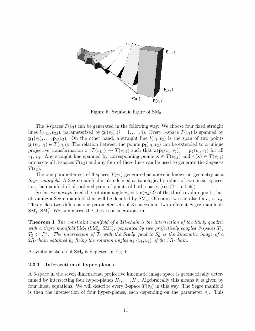
Figure 6: Symbolic figure of SM3

The 3-spaces T (v3) can be generated in the following way: We choose four fixed straightlines l(v1,i, v2,i), parameterized by pi(v3) (i = 1, . . . , 4). Every 3-space T (v3) is spanned byp1(v3), . . . ,p4(v3). On the other hand, a straight line l(v1, v2) is the span of two pointspj(v1, v2) ∈ T (v3,j). The relation between the points pj(v1, v2) can be extended to a uniqueprojective transformation π : T (v3,1) → T (v3,2) such that π(p1(v1, v2)) = p2(v1, v2) for allv1, v2. Any straight line spanned by corresponding points x ∈ T (v3,1) and π(x) ∈ T (v3,2)intersects all 3-spaces T (v3) and any four of these lines can be used to generate the 3-spacesT (v3).

The one parameter set of 3-spaces T (v3) generated as above is known in geometry as aSegre manifold. A Segre manifold is also defined as topological product of two linear spaces,i.e., the manifold of all ordered pairs of points of both spaces (see [21, p. 569]).

So far, we always fixed the rotation angle v3 = tan(u3/2) of the third revolute joint, thusobtaining a Segre manifold that will be denoted by SM3. Of course we can also fix v1 or v2.This yields two different one parameter sets of 3-spaces and two different Segre manifoldsSM′

3, SM′′3. We summarize the above considerations in

Theorem 1 The constraint manifold of a 3R-chain is the intersection of the Study quadricwith a Segre manifold SM3 (SM′

3, SM′′3), generated by two projectively coupled 3-spaces T1,

T2 ⊂ P 7. The intersection of Ti with the Study quadric S26 is the kinematic image of a

2R-chain obtained by fixing the rotation angles u3 (u1, u2) of the 3R-chain.

A symbolic sketch of SM3 is depicted in Fig. 6.

2.3.1 Intersection of hyper-planes

A 3-space in the seven dimensional projective kinematic image space is geometrically deter-mined by intersecting four hyper-planes H1, . . . , H4. Algebraically this means it is given byfour linear equations. We will describe every 3-space T (v3) in this way. The Segre manifoldis then the intersection of four hyper-planes, each depending on the parameter v3. This

11

representation will be used in the proposed algorithm for the inverse kinematics of an open6R-chain in Section 2.3.2.

For each of the four hyper-planes Hj(v3) four points pi(v3) are given; but they do notdetermine Hj(v3). Because seven points span a hyper-plane in P 7 we need three more pointsaj,1, aj,2, aj,3 ∈ Hj(v3) to compute a linear equation of Hj(v3). In principle, the points aj,k

can be taken anywhere in P 7 but it makes sense to choose them such that the resultinghyper-plane equations become as simple as possible. Without loss of generality we take thethree points such that aj,k ∈ SM3 ∩ S2

6 . We choose the points aj,k independent of v3; thereexist fixed parameter values vjk

3 such that aj,k ∈ T (vjk3 ).

The points pi(v3) and aj,k have coordinate vectors

pi(v3) = [pi0, . . . , pi7]T , aj,k =

[ajk

0 , . . . , ajk7

]T.

Note that the coordinates of pi depend linearly on v3, although this does not reflect in ournotation. The equation of a hyper-plane Hj(v3) is given by the Grassmannian determinant

Hj(v3) : det

x0 x1 x2 x3 y0 y1 y2 y3

p10 p11 p12 p13 p14 p15 p16 p17...

...p40 p41 p42 p43 p44 p45 p46 p47

aj10 aj1

1 aj12 aj1

3 aj14 aj1

5 aj16 aj1

7

aj20 aj2

1 aj22 aj2

3 aj24 aj2

5 aj26 aj2

7

aj30 aj3

1 aj32 aj3

3 aj34 aj3

5 aj36 aj3

7

= 0. (17)

We denote the coefficients of the hyperplane equations (17) by cjl, i.e.,

Hj(v3) : cj0x0 + cj1x1 + cj2x2 + cj3x3 + cj4y0 + cj5y1 + cj6y2 + cj7y3 = 0. (18)

The coefficients cjl are polynomials of degree four in v3 and can be interpreted as homoge-neous coordinates for the hyperplane Hj. Because of the special choice of the points aj,k,the polynomials cjl have the common divisor

g = (v3 − vj13 )(v3 − vj2

3 )(v3 − vj33 ). (19)

Dividing the polynomials cjl by g yields hyperplane coordinates for Hj(v3) that dependlinearly on v3. We state this as

Theorem 2 The Segre manifold SM3 is the intersection of four one parameter pencils ofhyperplanes Hj(v3). The hyperplane coordinates of Hj(v3) depend linearly on v3.

Remark 2 It is even possible to compute symbolically the hyperplane coordinates of Hj(v3)without specifying the DH-parameters of the 3R-robot. Computed once the equations can betaken for every possible design.

12

Figure 7: Cutting of the 6R into two 3R serial chains

2.3.2 Discussion of the Inverse Kinematics of General 6R-Manipulators

In this subsection we show how the constraint manifolds of 3R-chains can be used to solve theinverse kinematics of a general open 6R manipulator. Recall that in the inverse kinematicproblem of a serial chain the design and a pose of the end-effector of the manipulator isknown. The rotation angles ui of the revolute joints have to be computed. To apply thetheory developed in the last section we break up the link between the third and the fourthrevolute joint of the 6R and attach two copies of a coordinate frame ΣL = ΣR (the “left”and the “right” frame) in the middle of the common normal of these two joints such, thatthe twist angle between the z-axes of Σ3 and ΣL = ΣR is α3

2(Fig. 7). Then we compute the

direct kinematics for the first half of the 6R manipulator, which is now a 3R-chain, with theend-effector frame ΣL.

When the end-effector of the 6R manipulator is fixed we can do the same with the secondpart of the 6R but in the opposite direction. This means that for this 3R manipulator Σ6 isthe base and ΣR is the end-effector frame.

SM3,L is a Segre manifold in P 7. We saw that SM3,L is the intersection of four one-parameter sets of hyperplanes. The same is true for SM3,R. Hence, we have to intersecteight one parameter sets of hyper-planes with S2

6 . We summarize these results in

Theorem 3 Geometrically the inverse kinematics of a general 6R-serial chain is equivalentto the intersection of eight one parameter sets of hyper-planes with S2

6 .

An investigation of the algebraic structure of the nine equations reveals the non linearityof the problem. We have eight hyper-plane equations Hi(v3) = 0, Hi+4(v6) = 0, i = 1, . . . , 4and Equation (4) of S2

6 . The equations Hi are linear in xi, yi and bilinear in xiv3 and yiv3

13

resp. xiv6 and yiv6. The solution algorithm of this system is straight forward. The completesolution can be found in [16].

3 Synthesis of MechanismKinematic mapping can also be used in the synthesis of mechanisms. A detailed introductioninto this interesting topic can be found in [18]. The mathematical tools used there are closelyrelated to the presented methods within this paper. But there is a difference in the geometricinterpretation of the devised equations. We show the application of our methods in thesynthesis of a Bennett mechanism.

Figure 8: Bennett mechanism

The Bennett mechanism is a closed 4R-chain. It is well known that a Bennett mechanismcan be synthesized exactly when three poses of the end effector system are given (Fig.8).Synthesis means that we have to find the design parameters of the mechanism and thelocation of the axes in the fixed system and the location of the moving body in the movingsystem. For the synthesis of such a mechanism we attach two of the revolute axes to thefixed system and two axes to the moving (coupler) system. Now we prize open the couplerlink and obtain two open RR-chains. The basic idea of the synthesis is now: We map thepossible displacements of the first RR-chain onto S2

6 . This yields the constraint manifoldM1 of the RR-chain in the kinematic image space. The same procedure we perform withthe other RR-chain and obtain a second constraint manifold M2. Possible assembly modesof the two RR-chains correspond to intersection points of M1 and M2.

14

3.1 Constraint Manifold of RR-Chains

Using the Denavit-Hartenberg notation we compute the forward kinematics of the RR-chain.This yields a coordinate transformation of the type

x′(u1, u2) = A(u1, u2)x + t(u1, u2). (20)

u1 and u2 are the rotation parameters of the two rotations about the axes of the RR-chain.We apply the procedure explained in Section 1.1 to obtain the Study-parameters which arein this case functions of two parameters u1, u2:

xi = fi(u1, u2), yi = gi(u1, u2), i = 0, . . . 3. (21)

Elimination of the two parameters yields five equations in the unknowns xi, yi, i = 0, . . . , 3.It turns out that four equations are linear and one equation is the equation of the Study-quadric S2

6 . This result agrees with Selig [23], who derived a normal form of the equationsusing dual quaternions and exponential mapping. The multidimensional interpretation of thefive equations is as follows: each linear equation describes a (six dimensional) hyperplaneL6 of P 7. The intersection of these hyper-planes is a linear three-plane L3. This meansthat all possible poses of the end-effector of the RR-chain are in L3. Note that not allL3 ⊂ P 7 correspond to RR-chains. The constraint manifold M of an RR-chain is thereforethe intersection of L3 and S2

6 .With this knowledge we have a much simpler algorithm to derive the five linear equations

describing M: Each three-plane (i.e. a three dimensional space) is determined by fourpoints. To find the four linear equations we choose four discrete sets of rotation anglesui

1, ui2, i = 1, . . . , 4. These four sets correspond to four points Pi on the Study-quadric. Now

we construct four arbitrary hyper-planes L6 containing the four points Pi. This is done byadding three arbitrary points Qk

j , j = 1, . . . , 3, k = 1, . . . , 4 of P 7 different for each hyperplaneand computing the Grassmann determinant:

Ei =

∣∣∣∣∣∣x0 x1 x2 x3 y0 y1 y2 y3

pi0 pi1 pi2 pi3 pi4 pi5 pi6 pi7

qkj0 qk

j1 qkj2 qk

j3 qkj4 qk

j5 qkj6 qk

j7

∣∣∣∣∣∣ = 0, i = 1, . . . , 4, j = 1, . . . 3, k = 1, . . . , 4.

(22)Due to the fact that a Bennett mechanism consists of two RR-chains, one has to intersect

two three-planes L31, L3

2 in P 7. According to the well known dimension formula

dim(U ∩ V ) = dim(U) + dim(V )− dim(U + V ) (23)

where U, V denote sub-spaces of an n-dimensional space P n, the intersection of two three-planes L3

1, L32 in a seven dimensional space P 7 can be:

• dim(L31 ∩ L3

2) = −1,⇒ intersection is empty,

• dim(L31 ∩ L3

2) = 0,⇒ intersection is one point,

15

• dim(L31 ∩ L3

2) = 1,⇒ intersection is a line,

• dim(L31 ∩ L3

2) = 2,⇒ intersection is a two-plane

• dim(L31 ∩ L3

2) = 3 ⇒ L31 and L3

2 coincide.

The first case is the general case. The mechanical interpretation is that two general RR-chains never can be assembled to form a closed 4R-mechanism. There have to be conditionsto make this happen. When the constraint manifolds are chosen such that they come from a4R-chain, then they have exactly one point in common, which is on S2

6 (forward kinematicsof a serial 4R-chain). This fact is also a simple proof that the inverse kinematics of a general4R serial chain has one solution. The case of the line intersection is only possible for special4R-chains for which the inverse kinematics then has two solutions, which correspond to thetwo intersections of the line with S2

6 . As we know, the Bennett motion is a one-parameter-motion, represented by a curve in the kinematic image space. Therefore only the cases ofa line, which lies completely on S2

6 or a two-plane are of interest. The case that the lineis contained in S2

6 is not possible. Following Baker[2], who argued via screws, the relativemotion between opposite links of a proper Bennett loop can be neither purely rotationalnor purely translational at any time. Since straight lines on S2

6 correspond to rotations ortranslations we can restrict ourselves to the case of dim(L3

1 ∩ L32) = 2. The kinematic image

of the Bennett motion is therefore the intersection of a two-plane with the Study-quadricS2

6 . This yields another confirmation of the fact that the synthesis of a Bennett needs threeprecision points. Three precision points correspond to three points on the Study-quadricand span the two-plane. This agrees with [25]. Summarizing we have:

Theorem 4 Bennett motions are represented by planar sections of the Study-quadric andvice versa.

The intersection of the two-plane and S26 is a quadratic curve. In this sense Bennett mo-

tions can be regarded as the simplest non-trivial one parameter space motions. A directconsequence of the above considerations is the following

Corollary 1 Bennett linkages are the only movable 4R-chains.

It should be noted that to the authors’ best knowledge up to now there exist only complicatedalgebraic proofs of this result (see for example [17]). A complete discussion of the synthesisalgorithm including an example can be found in [7].

4 ConclusionIn this overview we have discussed the application of kinematic mapping and the resultinggeometric-algebraic approach to solve problems in mechanism analysis and synthesis. It wasshown that geometric preprocessing in a multidimensional setting allowed to simplify andsubsequently solve the sets of polynomial equations linked to the mechanical problems.

16

5 AcknowledgementsThe author is grateful to his colleagues H.-P. Schöcker, K. Brunnthaler and M. Pfurner forgiving the consent to use their results in this overview.

References[1] Angeles, J., Fundamentals of Robotic Mechanical Systems. Theory, Methods and Algo-

rithms, Springer, New York, 1997.

[2] Baker, J. E. 1998. On the motion geometry of the Bennett linkage. Proceedings ofthe 8th International Conference on Engineering Computer Graphics and DescriptiveGeometry. Austin. Texas. USA. pp. 433–437.

[3] Bennett, G. T. 1903. A new mechanism. Engineering. Vol. 76. pp. 777–778.

[4] Bennett, G. T. 1913–1914. The scew isogram-mechanism. Proceedings of the LondonMathematical Society. Vol. 13. pp. 151–173.

[5] Blaschke, W. 1960, Kinematik und Quaternionen, Wolfenbüttler Verlagsanstalt.

[6] Bottema, O., Roth, B., 1990, Theoretical Kinematics, Dover Publishing.

[7] Brunnthaler, K., Schröcker, H.-P., Husty, M. L., A new method for the synthesis ofBennet mechanisms, in: Proceedings of CK 2005, Cassino, Italy, 2005.

[8] Dickenstein, A. Emiris, I.Z., Solving Polynomial Equations, Foundations, Algorithmsand Applications, Springer Pub., 2005.

[9] Griffis, M., Crane, C., Duffy, J., 1994, ”A smart kinestatic interactive platform”, in:Lenarcic, J. and Ravani, B.: Advances in Robot Kinematics, Kluwer Acad. Pub., 459 –464, ISBN 0-7923-2983-X.

[10] Griffis, M., Duffy, J., 1993, "Method and Apparatus for Controlling Geometrically Sim-ple Parallel Mechanisms with Distinctive Connections", US Patent # 5,179, 525, 1993.

[11] Harris, J. , Algebraic Geometry: A First Course, Vol. 133 of Graduate Texts in Math-ematics, Springer, 1995.

[12] Husty, M. L., 1996, "An Algorithm for Solving the Direct Kinematic of General Stewart-Gough Platforms",Mechanism and Machine Theory, vol. 31, No. 4, pp. 365-380.

[13] Husty, M. L., Karger A., Sachs H., Steinhilper W., Kinematik und Robotik, Springer-Verlag, Berlin, Heidelberg, New York, 1997.

17

[14] Husty, M.L„ and Karger, A., 2000 "Self-Motions of Griffis-Duffy Type Platforms", Pro-ceedings of IEEE conference on Robotics and Automation (ICRA 2000), San Francisco,7–12.

[15] Husty, M. L. - Pfurner, M. - Schröcker, H.P., A New and Efficient Algorithm for the In-verse kinematics of a General 6R, Proceedings of IDETEC/CIE 2005, DETEC/MECH-84745, 2005, 8p.

[16] Husty, M. L. - Pfurner, M. - SchrÖCker, H.P., A New and Efficient Algorithm for theInverse Kinematics of a General 6R, Mech. Mach. Theory, 2006, in print.

[17] Karger, A. 4-parametric robot-manipulators and the Bennett’s mechanism. Privatecommunication.

[18] McCarthy J.M., Geometric Design of Linkages, Vol. 320 of Interdisciplinary AppliedMathematics, Springer-Verlag, New York, 2000.

[19] Mielczarek S., Husty M., - Hiller M., Designing a redundant Stewart-Gough platformwith a maximal forward kinematics solution set. CD-ROM, Proceedings MUSME, Mex-ico City, 12 pages, (2002).

[20] Merlet, J.P., 2000, Parallel Robots, Kluwer Academic Publishers, Dordrecht, TheNetherlands.

[21] Naas J., Schmid H., Mathematisches Wörterbuch, Vol. Band II, Akademie-Verlag Berlin,1974.

[22] Raghavan, M., 1991, "The Stewart platform of general geometry has 40 configurations",ASME Design and Automation Conf., Chicago, 1991, vol. 32-2, 397–402.

[23] Selig,J. M., Geometric Fundamentals of Robotics, Monographs in Computer Science,Springer, New York, 2005.

[24] Study E., Geometrie der Dynamen, B. G. Teubner, Leipzig, 1903.

[25] Suh, C. H., Radcliffe, C. W. 1978. Kinematics and Mechanisms Design. John Wileyand Sons. Canada.

[26] Wampler, C., 1996, "Forward displacement analysis of general six-in-parallel SPS (Stew-art) platform manipulators using soma coordinates", Mech. Mach. theory, vol.31 (3),331-337.

[27] Sommese, A, Verschelde, Wampler, Ch., 2002, ”Advances in Polynomial Continuationfor Solving problems in Kinematics”, preprint.

18