algebraic geometry
DESCRIPTION
A problem solving approachTRANSCRIPT
Algebraic Geometry: A Problem Solving
Approach
Park City Mathematics Institute - 2008
Thomas A. Garrity, Project Lead
Richard Belshoff
Lynette Boos
Ryan Brown
Jim Drouihlet
Carl Lienert
David Murphy
Junalyn Navarra-Madsen
Pedro Poitevin
Shawn Robinson
Brian A. Snyder
Caryn Werner
ii
Williams College
Missouri State University
Trinity College
Current address : Providence College
Georgia College and State University
Minnesota State University
Current address : Jim passed away January 23, 2009 during writing of this
book.
Fort Lewis College
Hillsdale College
Texas Woman’s University
Salem State College
University of Maine, Presque Isle
Lake Superior State University
Allegheny College


Contents
Preface ix
0.1. Algebraic geometry ix
0.2. Overview x
0.3. Problem book xi
0.4. History of book xii
0.5. An aside on notation xii
0.6. Thanks xiii
Chapter 1. Conics 1
1.1. Conics over the Reals 1
1.2. Changes of Coordinates 5
1.3. Conics over the Complex Numbers 14
1.4. The Complex Projective Plane P2 18
1.5. Projective Change of Coordinates 22
1.6. The Complex Projective Line P1 24
1.7. Ellipses, Hyperbolas, and Parabolas as Spheres 26
1.8. Degenerate Conics - Crossing lines and double lines. 30
1.9. Tangents and Singular Points 32
1.10. Conics via linear algebra 37
1.11. Duality 42
Chapter 2. Cubic Curves and Elliptic Curves 47
2.1. Cubics in C2 47
2.2. Inflection Points 48
2.3. Group Law 56
2.4. Normal forms of cubics 64
2.5. The Group Law for a Smooth Cubic in Canonical Form 75
2.6. Cubics as Tori 81
2.7. Cross-Ratios and the j-Invariant 83
2.8. Cross Ratio: A Projective Invariant 88
2.9. Torus as C/Λ 90
2.10. Mapping C/Λ to a Cubic 95
v

vi CONTENTS
Chapter 3. Higher Degree Curves 99
3.1. Higher Degree Polynomials and Curves 99
3.2. Higher Degree Curves as Surfaces 100
3.3. Bezout’s Theorem 104
3.4. Regular Functions and Function Fields 114
3.5. The Riemann-Roch Theorem 119
3.6. Blowing up 142
Chapter 4. Affine Varieties 149
4.1. Zero Sets of Polynomials 149
4.2. Algebraic Sets 151
4.3. Zero Sets via V (I) 152
4.4. Functions on Zero Sets and the Coordinate Ring 154
4.5. Hilbert Basis Theorem 155
4.6. Hilbert Nullstellensatz 157
4.7. Variety as Irreducible Algebraic Set: Prime Ideals 159
4.8. Subvarieties 161
4.9. Function Fields 163
4.10. Points as Maximal Ideals 165
4.11. The Zariski Topology 165
4.12. Points and Local Rings 172
4.13. Tangent Spaces 175
4.14. Dimension 180
4.15. Singular Points 182
4.16. Morphisms 185
4.17. Isomorphisms of Varieties 187
4.18. Rational Maps 191
4.19. Products of Affine Varieties 196
Chapter 5. Projective Varieties 199
5.1. Definition of Projective n-space Pn(k) 199
5.2. Graded Rings and Homogeneous Ideals 202
5.3. Projective Varieties 205
5.4. Functions on Projective Varieties 208
5.5. Examples 212
Chapter 6. Sheaves and Cohomology 217
6.1. Intuition and Motivation for Sheaves 217
6.2. The Definition of a Sheaf 220
6.3. The Sheaf of Rational Functions 224

CONTENTS vii
6.4. Divisors 225
6.5. Invertible Sheaves and Divisors 228
6.6. Basic Homology Theory 231
6.7. Cech Cohomology 232
Appendix A. A Brief Review of Complex Analysis 239
A.1. Visualizing Complex Numbers 239
A.2. Power Series 239
A.3. Residues 239
A.4. Liouville’s Theorem 239
Appendix. Bibliography 241
Appendix. Index 243


Preface
0.1. Algebraic geometry
As the name suggests, algebraic geometry is the linking of algebra to geometry.
For example, the circle, a geometric object, can also be described as the points
(1, 0)
(0, 1)
Figure 1. The unit circle centered at the origin
(x, y) in the plane satisfying the polynomial
x2 + y2 − 1 = 0,
an algebraic object. Algebraic geometry is thus often described as the study of
those geometric objects that can be described by polynomials. Ideally, we want a
complete correspondence between the geometry and the algebra, allowing intuitions
from one to shape and influence the other.
The building up of this correspondence is at the heart of much of mathematics
for the last few hundred years. It touches area after area of mathematics. By now,
despite the humble beginnings of the circle
(x2 + y2 − 1 = 0),
algebraic geometry is not an easy area to break into.
ix

x PREFACE
Hence this book.
0.2. Overview
Algebraic geometry is amazingly useful, and yet much of its development has
been guided by aesthetic considerations: some of the key historical developments
in the subject were the result of an impulse to achieve a strong internal sense of
beauty.
One way of doing mathematics is to ask bold questions about concepts you
are interested in studying. Usually this leads to fairly complicated answers having
many special cases. An important advantage of this approach is that the questions
are natural and easy to understand. A disadvantage is that, on the other hand, the
proofs are hard to follow and often involve clever tricks, the origin of which is very
hard to see.
A second approach is to spend time carefully defining the basic terms, with
the aim that the eventual theorems and their proofs are straightforward. Here,
the difficulty is in understanding how the definitions, which often initially seem
somewhat arbitrary, ever came to be. And the payoff is that the deep theorems are
more natural, their insights more accessible, and the theory is more aesthetically
pleasing. It is this second approach that has prevailed in much of the development
of algebraic geometry.
This second approach is linked to solving equivalence problems. By an equiva-
lence problem, we mean the problem of determining, within a certain mathematical
context, when two mathematical objects are the same. What is meant by the same
differs from one mathematical context to another. In fact, one way to classify
different branches of mathematics is to identify their equivalence problems.
A branch of mathematics is closed if its equivalence problems can be easily
solved. Active, currently rich branches of mathematics are frequently where there
are partial but not complete solutions. The branches of mathematics that will only
be active in the future are those for which there is currently no hint for solving any
type of equivalence problem.
To solve, or at least set up the language for a solution to an equivalence problem
frequently involves understanding the functions defined on an object. Since we will
be concerned with the algebra behind geometric objects, we will spend time on
correctly defining natural classes of functions on these objects. This in turn will
allow us to correctly describe what we will mean by equivalence.
Now for a bit of an overview of this text. In Chapter One, our motivation will
be to find the natural context for being able to state that all conics (all zero loci of
second degree polynomials) are the same. The key will be the development of the
complex projective plane P2. We will say that two curves in this new space P2 are

0.3. PROBLEM BOOK xi
the “same” (we will use the term “isomorphic”) if one curve can be transformed
into the other by a projective change of coordinates (which we will define).
Chapter Two will look at when two cubic curves are the same in P2 (meaning
again that one curve can be transformed into the other by a projective change of
coordinates). Here we will see that there are many, many different cubics. We will
further see that the points on a cubic have incredible structure; technically we will
see that the points form an abelian group.
Chapter Three turns to higher degree curves. From our earlier work, we still
think of these curves as “living” in the space P2. The first goal of this chapter
is Bezout’s theorem. If we stick to curves in the real plane R2, which would be
the naive first place to work in, one can prove that a curve that is the zero loci
of a polynomial of degree d will intersect another curve of degree e in at most de
points. In our claimed more natural space of P2, we will see that these two curves
will intersect in exactly de points, with the additional subtlety of needing to also
give the correct definition for intersection multiplicity. We will then define on a
curve its natural class of functions, which will be called the curve’s ring of regular
functions.
In Chapter Four we look at the geometry of more complicated objects than
curves in the plane P2. We will be treating the zero loci of collections of polynomials
in many variables, and hence looking at geometric objects in Cn. Here the exercises
work out how to bring much more of the full force of ring theory to bear on geometry;
in particular the function theory plays an increasingly important role. With this
language we will see that there are actually two different but natural equivalence
problems: isomorphism and birationality.
Chapter Five develops the true natural ambient space, complex projective n-
space Pn, and the corresponding ring theory.
Chapter Six moves up the level of mathematics, providing an introduction to
the more abstract (and more powerful) developments in algebraic geometry in the
nineteen fifties and nineteen sixties.
0.3. Problem book
This is a book of problems. We envision three possible audiences.
The first audience consists of students who have taken a courses in multivariable
calculus and linear algebra. The first three chapters are appropriate for a semester
long course for these people. If you are in this audience, here is some advice. You are
at the stage of your mathematical career of shifting from merely solving homework
exercises to proving theorems. While working the problems ask yourself what is the
big picture. After working a few problems, close the book and try to think of what
is going on. Ideally you would try to write down in your own words the material
xii PREFACE
that you just covered. What is most likely is that the first few times you try this,
you will be at a loss for words. This is normal. Use this as an indication that you
are not yet mastering this section. Repeat this process until you can describe the
mathematics with confidence, ready to lecture to your friends.
The second audience consists of students who have had a course in abstract
algebra. Then the whole book is fair game. You are at the stage where you know
that much of mathematics is the attempt to prove theorems. The next stage of
your mathematical development is in coming up with your own theorems, with the
ultimate goal being to become creative mathematicians. This is a long process.
We suggest that you follow the advice given in the previous paragraph, with the
additional advice being to occasionally ask yourself some of your own questions.
The third audience is what the authors referred to as “mathematicians on an
airplane.” Many professional mathematicians would like to know some algebraic
geometry. But jumping into an algebraic geometry text can be difficult. For the
pro, we had the image of them taking this book along on a long flight, with most of
the problems just hard enough to be interesting but not so hard so that distractions
on the flight will interfere with thinking. It must be emphasized that we do not
think of these problems as being easy for student readers.
0.4. History of book
This book, with its many authors, had its start in the summer of 2008 at the
Park City Mathematics Institute’s Undergraduate Faculty Program on Algebraic
and Analytic Geometry. Tom Garrity led a group of mathematicians on the the
basics of algebraic geometry, with the goal being for the participants to be able to
teach an algebraic geometry at their own college or university.
Since everyone had a Ph.D. in math, each of us knew that you cannot learn
math by just listening to someone lecture. The only way to learn is by thinking
through the math on ones own. Thus we decided to try to write a new beginning
text on algebraic geometry, based on the reader solving many, many exercises. This
book is the result.
0.5. An aside on notation
Good notation in mathematics is important but can be tricky. It is often the
case that the same mathematical object is best described using different notations
depending on context. For example, in this book we will sometimes denote a curve
by the symbol C while at other time denote the curve by the symbol V (P ), where
the curve is the zero loci of the polynomial P (x, y). Both notations are natural and
both will be used.

0.6. THANKS xiii
0.6. Thanks
There are going to be many people and organizations for which the authors are
grateful. We would like to thank the Institute for Advanced Study and the Park
City Mathematics Institute for their support.
The authors would like to thank the students at Georgia College and State
University who will course-test this manuscript and provide many great suggestions.

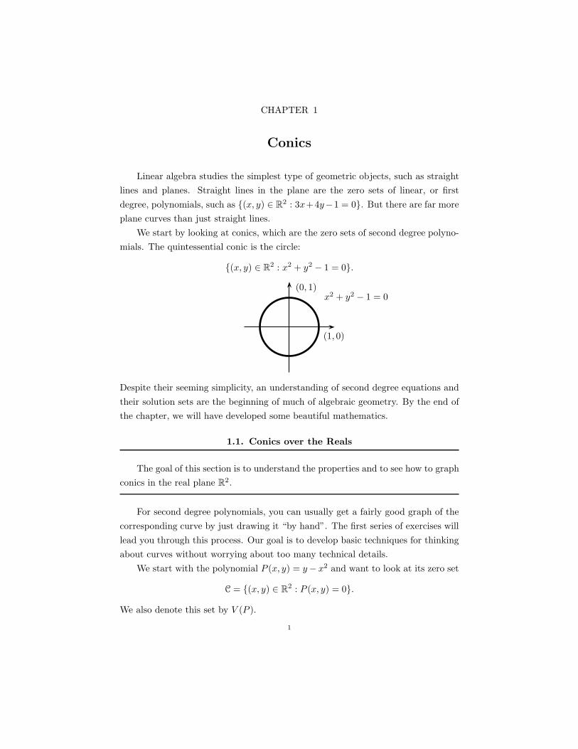
CHAPTER 1
Conics
Linear algebra studies the simplest type of geometric objects, such as straight
lines and planes. Straight lines in the plane are the zero sets of linear, or first
degree, polynomials, such as (x, y) ∈ R2 : 3x+4y−1 = 0. But there are far more
plane curves than just straight lines.
We start by looking at conics, which are the zero sets of second degree polyno-
mials. The quintessential conic is the circle:
(x, y) ∈ R2 : x2 + y2 − 1 = 0.
x2 + y2 − 1 = 0
(1, 0)
(0, 1)
Despite their seeming simplicity, an understanding of second degree equations and
their solution sets are the beginning of much of algebraic geometry. By the end of
the chapter, we will have developed some beautiful mathematics.
1.1. Conics over the Reals
The goal of this section is to understand the properties and to see how to graph
conics in the real plane R2.
For second degree polynomials, you can usually get a fairly good graph of the
corresponding curve by just drawing it “by hand”. The first series of exercises will
lead you through this process. Our goal is to develop basic techniques for thinking
about curves without worrying about too many technical details.
We start with the polynomial P (x, y) = y− x2 and want to look at its zero set
C = (x, y) ∈ R2 : P (x, y) = 0.
We also denote this set by V (P ).
1

2 1. CONICS
Exercise 1.1.1. Show that for any (x, y) ∈ C, then we also have
(−x, y) ∈ C.
Thus the curve C is symmetric about the y-axis.
Exercise 1.1.2. Show that if (x, y) ∈ C, then we have y ≥ 0.
Exercise 1.1.3. For points (x, y) ∈ C, show that if y goes to infinity, then
one of the corresponding x-coordinates also approaches infinity while the other
corresponding x-coordinate must approach negative infinity.
These two exercises show that the curve C is unbounded in the positive and
negative x-directions, unbounded in the positive y-direction, but bounded in the
negative y-direction. This means that we can always find (x, y) ∈ C so that x is
arbitrarily large, in either the positive or negative directions, y is arbitrarily large
in the positive direction, but that there is a number M (in this case 0) such that
y ≥M (in this case y ≥ 0).
Exercise 1.1.4. Sketch the curve C = (x, y) ∈ R2 : P (x, y) = 0. (The readeris welcome to use Calculus to give a more rigorous sketch of this curve.)
Conics that have these symmetry and boundedness properties and look like
this curve C are called parabolas. Of course, we could have analyzed the curve
(x, y) : x− y2 = 0 and made similar observations, but with the roles of x and y
reversed. In fact, we could have shifted, stretched, and rotated our parabola many
ways and still retained these basic features.
We now perform a similar analysis for the plane curve
C = (x, y) ∈ R2 :
(x2
4
)+
(y2
9
)− 1 = 0.
Exercise 1.1.5. Show that if (x, y) ∈ C, then the three points (−x, y), (x,−y),and (−x,−y) are also on C. Thus the curve C is symmetric about both the x and
y-axes.
Exercise 1.1.6. Show that for every (x, y) ∈ C, we have |x| ≤ 2 and |y| ≤ 3.
This shows that the curve C is bounded in both the positive and negative x
and y-directions.
Exercise 1.1.7. Sketch C = (x, y) ∈ R2 :
(x2
4
)+
(y2
9
)− 1 = 0.
Conics that have these symmetry and boundedness properties and look like this
curve C are called ellipses.
There is a third type of conic. Consider the curve
C = (x, y) ∈ R2 : x2 − y2 − 4 = 0.

1.1. CONICS OVER THE REALS 3
Exercise 1.1.8. Show that if (x, y) ∈ C, then the three points (−x, y), (x,−y),and (−x,−y) are also on C. Thus the curve C is also symmetric about both the x
and y-axes.
Exercise 1.1.9. Show that if (x, y) ∈ C, then we have |x| ≥ 2.
This shows that the curve C has two connected components. Intuitively, this
means that C is composed of two distinct pieces that do not touch.
Exercise 1.1.10. Show that the curve C is unbounded in the positive and
negative x-directions and also unbounded in the positive and negative y-directions.
Exercise 1.1.11. Sketch C = (x, y) ∈ R2 : x2 − y2 − 4 = 0.
Conics that have these symmetry, connectedness, and boundedness properties
are called hyperbolas.
In the following exercise, the goal is to sketch many concrete conics.
Exercise 1.1.12. Sketch the graph of each of the following conics in R2. Iden-
tify which are parabolas, ellipses, or hyperbolas.
(1) V (x2 − 8y)
(2) V (x2 + 2x− y2 − 3y − 1)
(3) V (4x2 + y2)
(4) V (3x2 + 3y2 − 75)
(5) V (x2 − 9y2)
(6) V (4x2 + y2 − 8)
(7) V (x2 + 9y2 − 36)
(8) V (x2 − 4y2 − 16)
(9) V (y2 − x2 − 9)
A natural question arises in the study of conics. If we have a second degree
polynomial, how can we determine whether its zero set is an ellipse, hyperbola,
parabola, or something else in R2. Suppose we have the following polynomial.
P (x, y) = ax2 + bxy + cy2 + dx + ey + h
What are there conditions on a, b, c, d, e, h that determine what type of conic V (P )
is? Whenever we have a polynomial in more than one variable, a useful technique
is to treat P as a polynomial in a single variable whose coefficients are themselves
polynomials.
Exercise 1.1.13. Express the polynomial P (x, y) = ax2+bxy+cy2+dx+ey+h
in the form
P (x, y) = Ax2 +Bx+ C
where A, B, and C are polynomial functions of y. What are A, B, and C?

4 1. CONICS
Since we are interested in the zero set V (P ), we want to find the roots of
Ax2 + Bx + C = 0 in terms of y. As we know from high school algebra not all
quadratic equations in a single variable have real roots. The number of real roots
is determined by the discriminant ∆x of the equation, so let’s find the discriminant
of Ax2 +Bx+ C = 0 as a function of y.
Exercise 1.1.14. Show that the discriminant of Ax2 +Bx+ C = 0 is
∆x(y) = (b2 − 4ac)y2 + (2bd− 4ae)y + (d2 − 4ah).
Exercise 1.1.15.
(1) Suppose ∆x(y0) < 0. Explain why there is no point on V (P ) whose
y-coordinate is y0.
(2) Suppose ∆x(y0) = 0. Explain why there is exactly one point V (P ) whose
y-coordinate is y0.
(3) Suppose ∆x(y0) > 0. Explain why there are exactly two points V (P )
whose y-coordinate is y0.
This exercise demonstrates that in order to understand the set V (P ) we need
to understand the set y | ∆x(y) ≥ 0.
Exercise 1.1.16. Suppose b2 − 4ac = 0.
(1) Show that ∆x(y) is linear and that ∆x(y) ≥ 0 if and only if y ≥ 4ah− d2
2bd− 4ae,
provided 2bd− 4ae 6= 0.
(2) Conclude that if b2 − 4ac = 0 (and 2bd − 4ae 6= 0) , then V (P ) is a
parabola.
Notice that if b2 − 4ac 6= 0, then ∆x(y) is itself a quadratic function in y,
and the features of the set over which ∆x(y) is nonnegative is determined by its
quadratic coefficient.
Exercise 1.1.17. Suppose b2 − 4ac < 0.
(1) Show that one of the following occurs: y | ∆x(y) ≥ 0 = ∅, y | ∆x(y) ≥0 = y0, or there exist real numbers α and β, α < β, such that y |∆x(y) ≥ 0 = y | α ≤ y ≤ β.
(2) Conclude that V (P ) is either empty, a point, or an ellipse.
Exercise 1.1.18. Suppose b2 − 4ac > 0.
(1) Show that one of the following occurs: y | ∆x(y) ≥ 0 = R and ∆x(y) 6=0, y | ∆x(y) = 0 = y0 and y | ∆x(y) > 0 = y | |y| > y0, or thereexist real numbers α and β, α < β, such that y | ∆x(y) ≥ 0 = y | y ≤α ∪ y | y ≥ β.

1.2. CHANGES OF COORDINATES 5
(2) Show that if there exist real numbers α and β, α < β, such that y |∆x(y) ≥ 0 = y | y ≤ α ∪ y | y ≥ β, then V (P ) is a hyperbola.
Above we decided to treat P as a function of x, but we could have treated P as
a function of y, P (x, y) = A′y2+B′y+C′ each of whose coefficients is a polynomial
in x.
Exercise 1.1.19. Show that the discriminant of A′y2 +B′y + C′ = 0 is
∆y(x) = (b2 − 4ac)x2 + (2be− 4cd)x+ (e2 − 4ch).
Note that the quadratic coefficient is again b2 − 4ac, so our observations from
above are the same in this case as well. In the preceding exercises we were inten-
tionally vague about some cases. For example, we do not say anything about what
happens when b2−4ac = 0 and 2bd−4ae = 0. This is an example of a “degenerate”
conic. We treat degenerate conics later in this chapter, but for now it suffices to
note that if b2 − 4ac = 0, then V (P ) is not an ellipse or hyperbola. If b2 − 4ac < 0,
then V (P ) is not a parabola or hyperbola. And if b2 − 4ac > 0, then V (P ) is not
a parabola or ellipse. This leads us to the following theorem.
Theorem 1.1.20. Suppose P (x, y) = ax2 + bxy+ cy2+ dx+ ey+h. If V (P ) is
a parabola in R2, then b2 − 4ac = 0; if V (P ) is an ellipse in R2, then b2 − 4ac < 0;
and if V (P ) is a hyperbola in R2, then b2 − 4ac > 0.
In general, it is not immediately clear whether a given conic V (ax2 + bxy +
cy2 + dx+ e + h) is an ellipse, hyperbola, or parabola, but if the coefficient b = 0,
then it is much easier to determine whether C = V (ax2 + cy2 + dx + ey + h) is an
ellipse, hyperbola, or parabola.
Corollary 1.1.1. Suppose P (x, y) = ax2 + cy2 + dx + ey + h. If V (P ) is a
parabola in R2, then ac = 0; if V (P ) is an ellipse in R2, then ac < 0, i.e. a and
c have opposite signs; and if V (P ) is a hyperbola in R2, then ac > 0, i.e. a and c
have the same sign.
1.2. Changes of Coordinates
The goal of this section is to sketch intuitively how, in R2, any ellipse can be
transformed into any other ellipse, any hyperbola into any other hyperbola, and
any parabola into any other parabola.
Here we start to investigate what it could mean for two conics to be the “same”;
thus we start to solve an equivalence problem for conics. Intuitively, two curves
are the same if we can shift, stretch, or rotate one to obtain the other. Cutting or
gluing however is not allowed.
6 1. CONICS
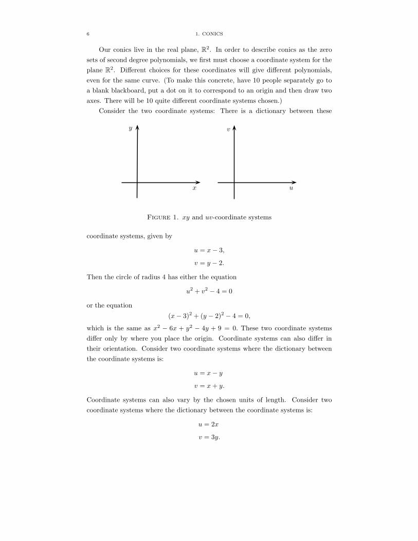
Our conics live in the real plane, R2. In order to describe conics as the zero
sets of second degree polynomials, we first must choose a coordinate system for the
plane R2. Different choices for these coordinates will give different polynomials,
even for the same curve. (To make this concrete, have 10 people separately go to
a blank blackboard, put a dot on it to correspond to an origin and then draw two
axes. There will be 10 quite different coordinate systems chosen.)
Consider the two coordinate systems: There is a dictionary between these
u
v
x
y
Figure 1. xy and uv-coordinate systems
coordinate systems, given by
u = x− 3,
v = y − 2.
Then the circle of radius 4 has either the equation
u2 + v2 − 4 = 0
or the equation
(x− 3)2 + (y − 2)2 − 4 = 0,
which is the same as x2 − 6x + y2 − 4y + 9 = 0. These two coordinate systems
differ only by where you place the origin. Coordinate systems can also differ in
their orientation. Consider two coordinate systems where the dictionary between
the coordinate systems is:
u = x− y
v = x+ y.
Coordinate systems can also vary by the chosen units of length. Consider two
coordinate systems where the dictionary between the coordinate systems is:
u = 2x
v = 3y.

1.2. CHANGES OF COORDINATES 7
u
v
4−4
4
−4
Figure 2. Circle of radius 4 centered at the origin in the uv-
coordinate system
x
y
u
v
Figure 3. xy and uv-coordinate systems with different orientations
All of these possibilities are captured in the following.
Definition 1.2.1. A real affine change of coordinates in the real plane, R2, is
given by
u = ax+ by + e
v = cx+ dy + f,
where a, b, c, d, e, f ∈ R and
ad− bc 6= 0.

8 1. CONICS
x
y
u
v
11
1
1
Figure 4. xy and uv-coordinate systems with different units
In matrix language, we have(u
v
)=
(a b
c d
)(x
y
)+
(e
f
),
where a, b, c, d, e, f ∈ R, and
det
(a b
c d
)6= 0.
Exercise 1.2.1. Show that the origin in the xy-coordinate system agrees with
the origin in the uv-coordinate system if and only if e = f = 0. Thus the constants
e and f describe translations of the origin.
Exercise 1.2.2. Show that if u = ax+ by+ e and v = cx+ dy+ f is a change
of coordinates, then the inverse change of coordinates is
x =
(1
ad− bc
)(du− bv)−
(1
ad− bc
)(de − bf)
y =
(1
ad− bc
)(−cu+ av)−
(1
ad− bc
)(−ce+ af).
This is why we require that ad − bc 6= 0. There are two ways of working this
problem. One method is to just start fiddling with the equations. The second is to
translate the change of coordinates into the matrix language and then use a little
linear algebra.
We frequently go back and forth between using a change of coordinates and its
inverse. For example, suppose we have the ellipse V (x2 + y2 − 1) in the xy-plane.
Under the real affine change of coordinates
u = x+ y
v = 2x− y,

1.2. CHANGES OF COORDINATES 9
this ellipse becomes V (5u2−2uv+2v2−9) in the uv-plane (verify this). To change
coordinates from the xy-plane to the uv-plane we replace x and y with u3 + v
4 and2u3 − v
3 , respectively. In other words to change from the xy-coordinate system to
the uv-coordinate system, we use the inverse change of coordinates
x =1
3u+
1
3v
y =2
3u− 1
3v.
Since any affine transformation has an inverse transformation, we will not worry too
much about whether we are using a transformation or its inverse in our calculations.
When the context requires care, we will make the distinction.
It is also common for us to change coordinates multiple times, but we need
to ensure that a composition of real affine changes of coordinates is a real affine
change of coordinates.
Exercise 1.2.3. Show that if
u = ax+ by + e
v = cx+ dy + f
and
s = Au+By + E
t = Cu+Dy + F
are two real affine changes of coordinates from the xy-plane to the uv-plane and
from the uv-plane to the st-plane, respectively, then the composition from the xy-
plane to the st-plane is a real affine change of coordinates.
Exercise 1.2.4. For each pair of ellipses, find a real affine change of coordinates
that maps the ellipse in the xy-plane to the ellipse in the uv-plane.
(1) V (x2 + y2 − 1), V (16u2 + 9v2 − 1)
(2) V ((x− 1)2 + y2 − 1), V (16u2 + 9(v + 2)2 − 1)
(3) V (4x2 + y2 − 6y + 8), V (u2 − 4u+ v2 − 2v + 4)
(4) V (13x2 − 10xy + 13y2 − 1), V (4u2 + 9v2 − 1)
We can apply a similar argument for hyperbolas.
Exercise 1.2.5. For each pair of hyperbolas, find a real affine change of coor-
dinates that maps the hyperbola in the xy-plane to the hyperbola in the uv-plane.

10 1. CONICS
(1) V (xy − 1), V (u2 − v2 − 1)
(2) V (x2 − y2 − 1), V (16u2 − 9v2 − 1)
(3) V ((x− 1)2 − y2 − 1), V (16u2 − 9(v + 2)2 − 1)
(4) V (x2 − y2 − 1), V (v2 − u2 − 1)
(5) V (8xy − 1), V (2u2 − 2v2 − 1)
Exercise 1.2.6. Give an intuitive argument, based on number of connected
components, for the fact that no ellipse can be transformed into a hyperbola by a
real affine change of coordinates.
Now we move on to parabolas.
Exercise 1.2.7. For each pair of parabolas, find a real affine change of coor-
dinates that maps the parabola in the xy-plane to the parabola in the uv-plane.
(1) V (x2 − y), V (9v2 − 4u)
(2) V ((x− 1)2 − y), V (u2 − 9(v + 2))
(3) V (x2 − y), V (u2 + 2uv + v2 − u+ v − 2).
(4) V (x2 − 4x+ y + 4), V (4u2 − (v + 1))
(5) V (4x2 + 4xy + y2 − y + 1), V (4u2 + v)
The preceding three problems suggest that we can transform ellipses to ellipses,
hyperbolas to hyperbolas, and parabolas to parabolas by way of real affine changes
of coordinates. This turns out to be the case. Suppose C = V (ax2+bxy+cy2+dx+
ey + h) is a smooth conic in R2. Our goal in the next several exercises is to show
that if C is an ellipse, we can transform it to V (x2 + y2 − 1); if C is a hyperbola, we
can transform it to V (x2 − y2 − 1); and if C is a parabola, we can transform it to
V (x2 − y). We will pass through a series of real affine transformations and appeal
to Exercise 1.2.3. This result ensures that the final composition of our individual
transformations is the real affine transformation we seek. This composition is,
however, a mess, so we won’t write it down explicitly. We will see in Section 1.10
that we can organize this information much more efficiently by using tools from
linear algebra.
We begin with ellipses. Suppose C = V (ax2 + bxy + cy2 + dx + ey + h) is an
ellipse in R2. Our first transformation will be to remove the xy term, i.e. to find a
real affine transformation that will align our given curve with the coordinate axes.
By Theorem 1.1.20 we know that b2 − 4ac < 0.
Exercise 1.2.8. Explain why if b2 − 4ac < 0, then ac > 0.

1.2. CHANGES OF COORDINATES 11
Exercise 1.2.9. Show that under the real affine transformation
x =
√c
au+ v
y = u−√a
cv
C in the xy-plane becomes an ellipse in the uv-plane whose defining equation is
Au2 + Cv2 + Du + Ev + H = 0. Find A and C in terms of a, b, c. Show that if
b2 − 4ac > 0, then A 6= 0 and C 6= 0.
Now we have a new ellipse V (Au2 + Cv2 +Du + Ev +H) in the uv-plane. If
our original ellipse already had b = 0, then we would have skipped the previous
step and gone directly to this one.
Exercise 1.2.10. Complete the square two times on the left hand side of the
equation
Au2 + Cv2 +Du+ Ev +H = 0
to rewrite this in the factored form
A(u−R)2 + C(v − S)2 − T = 0.
Express R, S, and T in terms of A,C,D,E, and H .
To simplify notation we revert our notation to x and y instead of u and v,
but we keep in mind that we are not really still working in our original xy-plane.
This is a convenience to avoid subscripts. Without loss of generality we can assume
A,C > 0, since if A,C < 0 we could simply multiply the above equation by −1
without affecting the conic. Note that we assume that our original conic is an
ellipse, i.e. it is nondegenerate. A consequence of this is that T 6= 0.
Exercise 1.2.11. Suppose A,C > 0. Find a real affine change of coordinates
that maps the ellipse
V (A(x −R)2 + C(y − S)2 − T ),
to the circle
V (u2 + v2 − 1).
Hence, we have found a (composition) real affine change of coordinates that
transforms any ellipse V (ax2+ bxy+ cy2+dx+ ey+h) to the circle V (u2+ v2− 1).
We can repeat this process in the case of parabolas.
Suppose C = V (ax2+bxy+cy2+dx+ey+h) is an parabola in R2. By Theorem
1.1.20 we know that b2 − 4ac = 0. As before our first task is to eliminate the xy
term. Suppose first that b 6= 0. Since b2 > 0 (b ∈ R) and 4ac = b2 we know ac > 0,
so we repeat Exercise 1.2.9.
12 1. CONICS
Exercise 1.2.12. Consider the values A and C found in Exercise 1.2.9. Show
that if b2 − 4ac = 0, then either A = 0 or C = 0, depending on the signs of a, b, c.
[Hint: Recall,√α2 = −α if α < 0.]
Since either A = 0 or C = 0 we can assume C = 0 without loss of generality, so
our transformed parabola is V (Au2+Du+Ev+H) in the uv-plane. If our original
parabola already had b = 0, then we also know, since b2 − 4ac, that either a = 0 or
c = 0, so we could have skipped ahead to this step.
Exercise 1.2.13. Complete the square on the left hand side of the equation
Au2 +Du+ Ev +H = 0
to rewrite this in the factored form
A(u−R)2 + E(v − T ) = 0.
Express R and T in terms of A,D, and H .
As above we revert our notation to x and y with the same caveat as before.
Exercise 1.2.14. Suppose A,B 6= 0. Find a real affine change of coordinates
that maps the parabola
V (A(x−R)2 − E(y − T )),
to the parabola
V (u2 − v).
Hence, we have found a (composition) real affine change of coordinates that
transforms any parabola V (ax2+bxy+cy2+dx+ey+h) to the parabola V (u2−v).Finally, suppose C = V (ax2 + bxy + cy2 + dx + ey + h) is a hyperbola in R2. By
Theorem 1.1.20 we know that b2− 4ac > 0. Suppose first that b 6= 0. Unlike before
we could have ac > 0, ac < 0, or ac = 0.
Exercise 1.2.15. Suppose ac > 0. Use the real affine transformation in Exer-
cise 1.2.9 to transform C to a conic in the uv-plane. Find the coefficients of u2 and
v2 in the resulting equation and show that they have opposite signs.
Exercise 1.2.16. Suppose ac < 0. Use the real affine transformation
x =
√− c
au+ v
y = u−√−acv
to transform C to a conic in the uv-plane. Find the coefficients of u2 and v2 in the
resulting equation and show that they have opposite signs.

1.2. CHANGES OF COORDINATES 13
Exercise 1.2.17. Suppose ac = 0 (so b 6= 0). Since either a = 0 or c = 0 we
can assume c = 0. Use the real affine transformation
x = u+ v
y = u− 2a
bv
to transform C = V (ax2 + bxy + dx+ ey + h) to a conic in the uv-plane. Find the
coefficients of u2 and v2 in the resulting equation and show that they have opposite
signs.
In all three cases we find the C is transformed to V (Au2−Cv2+Du+Ev+H)
in the uv-plane. We can now complete the hyperbolic transformation as we did
above with parabolas and ellipses.
Exercise 1.2.18. Complete the square two times on the left hand side of the
equation
Au2 − Cv2 +Du+ Ev +H = 0
to rewrite this in the factored form
A(u−R)2 − C(v − S)2 − T = 0.
Express R, S, and T in terms of A,C,D,E, and H .
Exercise 1.2.19. Suppose A,C > 0. Find a real affine change of coordinates
that maps the hyperbola
V (A(x −R)2 − C(y − S)2 − T ),
to the hyperbola
V (u2 − v2 − 1).
We have now shown that in R2 we can find a real affine change of coordinates
that will transform any ellipse to V (x2 + y2 − 1), any hyperbola to V (x2 − y2 − 1),
and any parabola to V (x2 − y). Thus we have three classes of smooth conics in R2.
Our next task is to show that these are distinct, that is, that we cannot transform
an ellipse to a parabola and so on.
Exercise 1.2.20. Give an intuitive argument, based on number of connected
components, for the fact that no ellipse can be transformed into a hyperbola by a
real affine change of coordinates.
Exercise 1.2.21. Show that there is no real affine change of coordinates
u = ax+ by + e
v = cx+ dy + f
that transforms the ellipse V (x2 + y2 − 1) to the hyperbola V (u2 − v2 − 1).
14 1. CONICS
Exercise 1.2.22. Give an intuitive argument, based on boundedness, for the
fact that no parabola can be transformed into an ellipse by a real affine change of
coordinates.
Exercise 1.2.23. Show that there is no real affine change of coordinates that
transforms the parabola V (x2 − y) to the circle V (u2 + v2 − 1).
Exercise 1.2.24. Give an intuitive argument, based on the number of con-
nected components, for the fact that no parabola can be transformed into a hyper-
bola by a real affine change of coordinates.
Exercise 1.2.25. Show that there is no real affine change of coordinates that
transforms the parabola V (x2 − y) to the hyperbola V (u2 − v2 − 1).
Definition 1.2.2. The zero loci of two conics are equivalent under a real affine
change of coordinates if the defining polynomial for one of the conics can be trans-
formed via a real affine change of coordinates into the defining polynomial of the
other conic.
Combining all of the work in this section, we have just proven the following
theorem.
Theorem 1.2.26. Under a real affine change of coordinates, all ellipses in R2
are equivalent, all hyperbolas in R2 are equivalent, and all parabolas in R2 are
equivalent. Further, these three classes of conics are distinct; no conic of one class
can be transformed via a real affine change of coordinates to a conic of a different
class.
In Section 1.10 we will revisit this theorem using tools from linear algebra.
This approach will yield a cleaner and more straightforward proof than the one
we have in the current setting. The linear algebraic setting will also make all of
our transformations simpler, and it will become apparent how we arrived at the
particular transformations.
1.3. Conics over the Complex Numbers
The goal of this section is to see how, under a complex affine changes of coordinates,
all ellipses and hyperbolas are equivalent, while parabolas are still distinct.
While it is certainly natural to begin with the zero set of a polynomial P (x, y)
as a curve in the real plane R2, polynomials also have roots over the complex
numbers. In fact, throughout mathematics it is almost always easier to work over
the complex numbers than over the real numbers. This can be seen even in the
solutions given by the quadratic equation, as seen in the following exercises:

1.3. CONICS OVER THE COMPLEX NUMBERS 15
Exercise 1.3.1. Show that x2+1 = 0 has no solutions if we require x ∈ R but
does have the two solutions, x = ±i, in the complex numbers C.
Exercise 1.3.2. Show that the set
(x, y) ∈ R2 : x2 + y2 = −1
is empty but that the set
C = (x, y) ∈ C2 : x2 + y2 = −1
is not empty. If fact, show that given any complex number x that there must exist
a y ∈ C such that
(x, y) ∈ C.
Then show that if x 6= ±i, then there are two distinct values y ∈ C such that
(x, y) ∈ C, while if x = ±i, there is only one such y.
Thus if we only allow a solution to be a real number, some zero sets of second
degree polynomials will be empty. This does not happen over the complex numbers.
Exercise 1.3.3. Let
P (x, y) = ax2 + bxy + cy2 + dx+ ey + f = 0,
with a 6= 0. Show that for any value y ∈ C, there must be at least one x ∈ C, butno more than two such x’s, such that
P (x, y) = 0.
[Hint: Write P (x, y) = Ax2 + Bx + C as a function of x whose coefficients A, B,
and C are themselves functions of y, and use the quadratic formula. This technique
will be used frequently.]
Thus for any second order polynomial, its zero set is non-empty provided we
work over the complex numbers.
But even more happens. We start with:
Exercise 1.3.4. Let C = V((
x2
4
)+(y2
9
)− 1)
⊂ C2. Show that C is un-
bounded in both x and y. (Over the complex numbers C, being unbounded in x,
say, means, given any numberM , there will be point (x, y) ∈ C such that |x| > M .)
Hyperbolas in R2 come in two pieces. In C2, it can be shown that hyperbolas
are connected, meaning there is a continuous path from any point to any other
point. The following shows this for a specific hyperbola.

16 1. CONICS
Exercise 1.3.5. Let C = V (x2−y2−0) ⊂ C2. Show that there is a continuous
path on the curve C from the point (−1, 0) to the point (1, 0), despite the fact that
no such continuous path exists in R2. (Compare this exercise with Exercise 1.1.9.)
Definition 1.3.1. A complex affine change of coordinates in the complex plane
C2 is given by
u = ax+ by + e
v = cx+ dy + f,
where a, b, c, d, e, f ∈ C and
ad− bc 6= 0.
Exercise 1.3.6. Show that if u = ax+ by+ e and v = cx+ dy+ f is a change
of coordinates, then the inverse change of coordinates is
x =
(1
ad− bc
)(du− bv)−
(1
ad− bc
)(de − bf)
y =
(1
ad− bc
)(−cu+ av)−
(1
ad− bc
)(−ce+ af).
This proof should look almost identical to the solution of Exercise 1.2.2.
Definition 1.3.2. The zero loci of two conics are equivalent under a complex
affine change of coordinates if the defining polynomial for one of the conics can be
transformed via a complex affine change of coordinates into the defining polynomial
for the other conic.
Exercise 1.3.7. Use Theorem 1.2.26 together with the new result of Exercise
1.3.6 to conclude that all ellipses and hyperbolas are equivalent under complex
affine changes of coordinates.
Parabolas, though, are still different:
Exercise 1.3.8. Show that (x, y) ∈ C2 : x2 + y2 − 1 = 0 is not equivalent
under a complex affine change of coordinates to the parabola (u, v) ∈ C2 : u2−v =
0.
We now want to look more directly at C2 in order to understand more clearly
why the class of ellipses and the class of hyperbolas are different as real objects but
the same as complex objects. We start by looking more closely at C. Algebraic
geometers regularly use the variable x for a complex number. Complex analysts
more often use the variable z, which allows a complex number to be expressed in
terms of its real and imaginary parts.
z = x+ iy,

1.3. CONICS OVER THE COMPLEX NUMBERS 17
x
y
1
1
C
b2 + i
b
−3− 2i
b
−3 + 4i
Figure 5. Points in the complex plane
where x is the real part of z and y is the imaginary part.
Similarly, an algebraic geometer will usually use (x, y) to denote points in the
complex plane C2 while a complex analyst will instead use (z, w) to denote points
in the complex plane C2. Here the complex analyst will write
w = u+ iv.
There is a natural bijection from C2 to R4 given by
(z, w) = (x+ iy, u+ iv) → (x, y, u, v).
In the same way, there is a natural bijection from C2∩(x, y, u, v) ∈ R4 : y = 0, v =
0 to the real plane R2, given by
(x+ 0i, u+ 0i) → (x, 0, u, 0) → (x, u).
Likewise, there is a similar natural bijection from C2 = (z, w) ∈ C2∩(x, y, u, v) ∈R4; y = 0, u = 0 to R2, given this time by
(x+ 0i, 0 + vi) → (x, 0, 0, v) → (x, v).
One way to think about conics in C2 is to consider two dimensional slices of
C2. Let
C = (z, w) ∈ C2 : z2 + w2 = 1.
Exercise 1.3.9. Give a bijection from
C ∩ (x+ iy, u+ iv) : x, u ∈ R, y = 0, v = 0
to the real circle of unit radius in R2. (Thus a real circle in the plane R2 can be
thought of as real slice of the complex curve C.)
Taking a different real slice of C will yield not a circle but a hyperbola.
18 1. CONICS
Exercise 1.3.10. Give a bijection from
C ∩ (x+ iy, u+ iv) ∈ R4 : x, v ∈ R, y = 0, u = 0
to the hyperbola (x2 − v2 = 1) in R2.
Thus the single complex curve C contains both real circles and real hyperbolas.
1.4. The Complex Projective Plane P2
The goal of this section is to introduce the complex projective plane P2, the natural
ambient space (with its higher dimensional analog Pn) for much of algebraic geom-
etry. In P2, we will see that all ellipses, hyperbolas and parabolas are equivalent.
In R2 all ellipses are equivalent, all hyperbolas are equivalent, and all parabolas
are equivalent under a real affine change of coordinates. Further, these classes
of conics are distinct in R2. When we move to C2 ellipses and hyperbolas are
equivalent under a complex affine change of coordinates, but parabolas remain
distinct. The next step is to understand the “points at infinity” in C2.
We will give the definition for the complex projective plane P2 together with
exercises to demonstrate its basic properties. It may not be immediately clear what
this definition has to do with the “ordinary” complex plane C2. We will then see
how C2 naturally lives in P2 and how the “extra” points in P2 that are not in C2
are viewed as points at infinity. In the next section we will look at the projective
analogue of change of coordinates and see how we can view all ellipses, hyperbolas
and parabolas as equivalent.
Definition 1.4.1. Define a relation ∼ on points in C3 − (0, 0, 0) as follows:
(x, y, z) ∼ (u, v, w) if and only if there exists λ ∈ C − 0 such that (x, y, z) =
(λu, λv, λw).
Exercise 1.4.1. Show that ∼ is an equivalence relation.
Exercise 1.4.2.
(1) Show that (2, 1 + i, 3i) ∼ (2 − 2i, 2, 3 + 3i).
(2) Show that (1, 2, 3) ∼ (2, 4, 6) ∼ (−2,−4,−6) ∼ (−i,−2i,−3i).
(3) Show that (2, 1 + i, 3i) 6∼ (4, 4i, 6i).
(4) Show that (1, 2, 3) (3, 6, 8).
Exercise 1.4.3. Suppose that (x1, y1, z1) ∼ (x2, y2, z2) and that x1 = x2. Show
then that y1 = y2 and z1 = z2.

1.4. THE COMPLEX PROJECTIVE PLANE P2 19
Exercise 1.4.4. Suppose that (x1, y1, z1) ∼ (x2, y2, z2) with z1 6= 0 and z2 6= 0.
Show that
(x1, y1, z1) ∼(x1z1,y1z1, 1
)∼(x2z2,y2z2, 1
)∼ (x2, y2, z2).
Let (x : y : z) denote the equivalence class of (x, y, z), i.e. (x : y : z) is the
following set.
(x : y : z) = (u, v, w) ∈ C3 − (0, 0, 0) : (x, y, z) ∼ (u, v, w)
Exercise 1.4.5. (1) Find the equivalence class of (0, 0, 1).
(2) Find the equivalence class of (1, 2, 3).
Exercise 1.4.6. Show that the equivalence classes (1 : 2 : 3) and (2 : 4 : 6) are
equal as sets.
Definition 1.4.2. The complex projective plane, P2(C), is the set of equiva-
lence classes of the points in C3 − (0, 0, 0). That is,
P2(C) =(C3 − (0, 0, 0)
)/∼ .
The set of points (x : y : z) ∈ P2(C) : z = 0 is called the line at infinity. We will
write P2 to mean P2(C) when the context is clear.
Let (a, b, c) ∈ C3 − (0, 0, 0). Then the complex line through this point and
the origin (0, 0, 0) can be defined as all points, (x, y, z), satisfying
x = λa, y = λb, and z = λc,
for any complex number λ. Here λ can be thought of as an independent parameter.
Exercise 1.4.7. Explain why the elements of P2 can intuitively be thought of
as complex lines through the origin in C3.
Exercise 1.4.8. If c 6= 0, show, in C3, that the line x = λa, y = λb, z = λc
intersects the plane (x, y, z) : z = 1 in exactly one point. Show that this point of
intersection is(ac ,
bc , 1).
In the next several exercises we will use
P2 = (x : y : z) ∈ P2 : z 6= 0 ∪ (x : y : z) ∈ P2 : z = 0
to show that P2 can be viewed as the union of C2 with the line at infinity.
Exercise 1.4.9. Show that the map φ : C2 → (x : y : z) ∈ P2 : z 6= 0 defined
by φ(x, y) = (x : y : 1) is a bijection.
Exercise 1.4.10. Find a map from (x : y : z) ∈ P2 : z 6= 0 to C2 that is the
inverse of the map φ in Exercise 1.4.9.

20 1. CONICS
The maps φ and φ−1 in Exercises 1.4.9 and 1.4.10 show us how to view C2
inside P2. Now we show how the set (x : y : z) ∈ P2 : z = 0 corresponds to
directions towards infinity in C2.
Exercise 1.4.11. Consider the line ` = (x, y) ∈ C2 : ax+ by + c = 0 in C2.
Assume a, b 6= 0. Explain why, as |x| → ∞, |y| → ∞. (Here, |x| is the modulus of
x.)
Exercise 1.4.12. Consider again the line `. We know that a and b cannot
both be 0, so we will assume without loss of generality that b 6= 0.
(1) Show that the image of ` in P2 under φ is the set
(bx : −ax− c : b) : x ∈ C.
(2) Show that this set equals the following union.
(bx : −ax− c : b) : x ∈ C = (0 : −c : b) ∪(
1 : −ab− c
bx:1
x
)
(3) Show that as |x| → ∞, the second set in the above union becomes
(1 : −ab: 0).
Thus, the points (1 : −ab : 0) are directions toward infinity and the set (x : y : z) ∈
P2 : z = 0 is the line at infinity.
If a point (a : b : c) in P2 is the image of a point (x, y) ∈ C2 under the map
from C2 φ−→ P2, we say that (a, b, c) ∈ C3 are the homogeneous coordinates for (x, y).
Notice that the homogeneous coordinates for a point (x, y) ∈ C2 are not unique.
For example, the coordinates (2 : −3 : 1), (10 : −15 : 5), and (2−2i : −3+3i : 1− i)are all homogeneous coordinates for (2,−3).
In order to consider zero sets of polynomials in P2, a little care is needed. We
start with:
Definition 1.4.3. A polynomial is homogeneous if every monomial term has
the same total degree, that is, if the sum of the exponents in every monomial is
the same. The degree of the homogeneous polynomial is the degree of one of its
monomials. An equation is homogeneous if every nonzero monomial has the same
total degree.
Exercise 1.4.13. Explain why the following polynomials are homogeneous,
and find each degree.
(1) x2 + y2 − z2
(2) xz − y2
(3) x3 + 3xy2 + 4y3
(4) x4 + x2y2

1.4. THE COMPLEX PROJECTIVE PLANE P2 21
Exercise 1.4.14. Explain why the following polynomials are not homogeneous.
(1) x2 + y2 − z
(2) xz − y
(3) x2 + 3xy2 + 4y3 + 3
(4) x3 + x2y2 + x2
Exercise 1.4.15. Show that if the homogeneous equation Ax +By + Cz = 0
holds for the point (x, y, z) in C3, then it holds for every point of C3 that belongs
to the equivalence class (x : y : z) in P2.
Exercise 1.4.16. Show that if the homogeneous equation Ax2 +By2 +Cz2 +
Dxy + Exz + Fyz = 0 holds for the point (x, y, z) in C3, then it holds for every
point of C3 that belongs to the equivalence class (x : y : z) in P2.
Exercise 1.4.17. State and prove the generalization of the previous two exer-
cises for any degree n homogeneous equation P (x, y, z) = 0.
Exercise 1.4.18. Consider the non-homogeneous equation P (x, y, z) = x2 +
2y + 2z = 0. Show that (2,−1,−1) satisfies this equation, but not all other points
of the equivalence class (2 : −1 : −1) satisfy the equation.
Thus the zero set of a non-homogeneous polynomials is not well- defined in P2.
These exercises demonstrate that the only polynomials that are well-defined on P2
(and any projective space Pn) are homogeneous polynomials.
In order to study the behavior at infinity of a curve in C2, we would like
to extend the curve to P2. In order for the zero set of a polynomial over P2 to
be well-defined we must, for any given a polynomial on C2, replace the original
(possibly non-homogeneous) polynomial with a homogeneous one. For any point
(x : y : z) ∈ P2 with z 6= 0 we have (x : y : z) ∼(xz : yz : 1
)which we identify, via
φ−1 from Exercise 1.4.10, with the point(xz ,
yz
)∈ C2. This motivates our procedure
to homogenize polynomials.
We start with an example. With a slight abuse of notation, the polynomial
P (x, y) = y − x − 2 maps to P (x, y, z) = yz − x
z − 2. Since P (x, y, z) = 0 and
zP (x, y, z) = 0 have the same zero set if z 6= 0 we clear the denominator and
consider the polynomial P (x, y, z) = y−x−2z. The zero set of P (x, y, z) = y−x−2z
in P2 corresponds to the zero set of P (x, y) = y − x − 2 = 0 in C2 precisely when
z = 1.
Similarly, the polynomial x2 + y2 − 1 maps to(xz
)2+(yz
)2 − 1. Again, clear
the denominators to obtain the homogeneous polynomial x2 + y2 − z2, whose zero
set, V (x2 + y2 − z2) ⊂ P2 corresponds to the zero set, V (x2 + y2 − 1) ⊂ C2 when
z = 1.

22 1. CONICS
Definition 1.4.4. Let P (x, y) be a degree n polynomial defined over C2. The
corresponding homogeneous polynomial defined over P2 is
P (x, y, z) = znP(xz,y
z
).
Exercise 1.4.19. Homogenize the following equations. Then find the point(s)
where the curves intersect the line at infinity.
(1) ax+ by + c = 0
(2) x2 + y2 = 1
(3) y = x2
(4) x2 + 9y2 = 1
(5) y2 − x2 = 1
Exercise 1.4.20. Show that in P2, any two distinct lines will intersect in a
point. Notice, this implies that parallel lines in C2, when embedded in P2, intersect
at the line at infinity.
Exercise 1.4.21. Once we have homogenized an equation, the original vari-
ables x and y are no more important than the variable z. Suppose we regard x
and z as the original variables in our homogenized equation. Then the image of the
xz-plane in P2 would be (x : y : z) ∈ P2 : y = 1.(1) Homogenize the equations for the parallel lines y = x and y = x+ 2.
(2) Now regard x and z as the original variables, and set y = 1 to sketch the
image of the lines in the xz-plane.
(3) Explain why the lines in part (2) meet at the x−axis.
1.5. Projective Change of Coordinates
The goal of this section is to define a projective change of coordinates and then
show that all ellipses, hyperbolas and parabolas are equivalent under a projective
change of coordinates.
Earlier we described a complex affine change of coordinates from C2 with points
(x, y) to C2 with points (u, v) by setting u = ax+ bx+ e and v = cx+ dy + f . We
will define the analog for changing homogeneous coordinates (x : y : z) for some
P2 to homogeneous coordinates (u : v : w) for another P2. We need the change of
coordinates equations to be both homogeneous and linear:
Definition 1.5.1. A projective change of coordinates is given by
u = a11x+ a12y + a13z
v = a21x+ a22y + a23z
w = a31x+ a32y + a33z

1.5. PROJECTIVE CHANGE OF COORDINATES 23
where the aij ∈ C and
det
a11 a12 a13
a21 a22 a23
a31 a32 a33
6= 0.
In matrix language u
v
w
= A
x
y
z
,
where A = (aij), aij ∈ C, and detA 6= 0.
Definition 1.5.2. Two conics in P2 are equivalent under a projective change
of coordinates, or projectively equivalent, if the defining homogeneous polynomial
for one of the conics can be transformed into the defining polynomial for the other
conic via a projective change of coordinates.
Exercise 1.5.1. For the complex affine change of coordinates
u = ax+ by + e
v = cx+ dy + f,
where a, b, c, d, e, f ∈ C and ad− bc 6= 0, show that
u = ax+ by + ez
v = cx+ dy + fz
w = z
is the corresponding projective change of coordinates.
This means that if two conics in C2 are equivalent under a complex affine
change of coordinates, then the corresponding conics in P2 will still be equivalent,
but now under a projective change of coordinates.
Exercise 1.5.2. Let C1 = V (x2 + y2 − 1) be an ellipse in C2 and let C2 =
V (u2 − v) be a parabola in C2. Homogenize the defining polynomials for C1 and
C2 and show that the projective change of coordinates
u = ix
v = y + z
w = y − z
transforms the ellipse in P2 into the parabola in P2.
Exercise 1.5.3. Use the results of Section 1.3 together with the above problem
to show that, under a projective change of coordinates, all ellipses, hyperbolas, and
parabolas are equivalent in P2.
24 1. CONICS
1.6. The Complex Projective Line P1
The goal of this section is to define the complex projective line P1 and show that it
can be viewed topologically as a sphere. In the next section we will use this to show
that ellipses, hyperbolas, and parabolas are also spheres in the complex projective
plane P2.
We start with the definition of P1:
Definition 1.6.1. Define an equivalence relation ∼ on points in C2 − (0, 0)as follows: (x, y) ∼ (u, v) if and only if there exists λ ∈ C− 0 such that (x, y) =
(λu, λv). Let (x : y) denote the equivalence class of (x, y). The complex projective
line P1 is the set of equivalence classes of points in C2 − (0, 0). That is,
P1 =(C2 − (0, 0)
)/∼ .
The point (1 : 0) is called the point at infinity.
The next series of problems are direct analogs of problems for P2.
Exercise 1.6.1. Suppose that (x1, y1) ∼ (x2, y2) and that x1 = x2 6= 0. Show
that y1 = y2.
Exercise 1.6.2. Suppose that (x1, y1) ∼ (x2, y2) with y1 6= 0 and y2 6= 0.
Show that
(x1, y1) ∼(x1y1, 1
)∼(x2y2, 1
)∼ (x2, y2).
Exercise 1.6.3. Explain why the elements of P1 can intuitively be thought of
as complex lines through the origin in C2.
Exercise 1.6.4. If b 6= 0, show, in C2, that the line x = λa, y = λb will
intersect the plane (x, y) : y = 1 in exactly one point. Show that this point of
intersection is(ab , 1).
We have that
P1 = (x : y) ∈ P1 : y 6= 0 ∪ (1 : 0).
Exercise 1.6.5. Show that the map φ : C→ (x : y) ∈ P1 : y 6= 0 defined by
φ(x) = (x : 1) is a bijection.
Exercise 1.6.6. Find a map from (x : y) ∈ P1 : y 6= 0 to C that is the
inverse of the map φ in Exercise 1.6.5.

1.6. THE COMPLEX PROJECTIVE LINE P1 25
The maps φ and φ−1 in Exercises 1.6.5 and 1.6.6 show us how to view C inside
P1. Now we want to see how the extra point (1 : 0) will correspond to the point at
infinity of C.
inverse of the map in the previous problem.
Exercise 1.6.7. Consider the map φ : C → P1 given by φ(x) = (x : 1). Show
that as |x| → ∞, we have φ(x) → (1 : 0).
Hence we can think of P1 as the union of C and a single point at infinity. Now
we want to see how we can regard P1 as a sphere, which means we want to find a
homeomorphism between P1 and a sphere. A homeomorphism is a continuous map
with a continuous inverse. Two spaces are topologically equivalent, or homeomor-
phic, if we can find a homeomorphism from one to the other. We know that the
points of C are in one-to-one correspondence with the points of the real plane R2,
so we will first work in R2 ⊂ R3. Let S2 denote the unit sphere in R3 centered at
the origin. This sphere is given by the equation
x2 + y2 + z2 = 1.
Exercise 1.6.8. Let p denote the point (0, 0, 1) ∈ S2, and let ` denote the line
through p and the point (x, y, 0) in the xy-plane, whose parametrization is given
by
γ(t) = (1 − t)(0, 0, 1) + t(x, y, 0),
i.e.
l = (tx, ty, 1− t) | t ∈ R.(1) ` clearly intersects S2 at the point p. Show that there is exactly one other
point of intersection q.
(2) Find the coordinates of q.
(3) Define the map ψ : R2 → S2 − p to be the map that takes the point
(x, y) to the point q. Show that ψ is a continuous bijection.
(4) Show that as |(x, y)| → ∞, we have ψ(x, y) → p.
The above argument does establish a homeomorphism, but it relies on coordi-
nates and an embedding of the sphere in R3. We now give an alternative method
for showing that P1 is a sphere that does not rely as heavily on coordinates.
If we take a point (x : y) ∈ P1, then we can choose a representative for this
point of the form(xy : 1
), provided y 6= 0, and a representative of the form
(1 : yx
),
provided x 6= 0.
Exercise 1.6.9. Determine which point(s) in P1 do not have two representa-
tives of the form (x : 1) = (1 : 1x ).

26 1. CONICS
Our constructions needs two copies of C. Let U denote the first copy of C,
whose elements are denoted by x. Let V be the second copy of C, whose elements
we’ll denote y. Further let U∗ = U − 0 and V ∗ = V − 0.
Exercise 1.6.10. Map U → P1 via x→ (x : 1) and map V → P1 via y → (1 :
y). Show that there is a the natural one-to-one map U∗ → V ∗.
The next two exercises have quite a different flavor than most of the problems
in the book. The emphasis is not on calculations but on the underlying intuitions.
Exercise 1.6.11. A sphere can be split into a neighborhood of its northern
hemisphere and a neighborhood of its southern hemisphere. Show that a sphere
can be obtained by correctly gluing together two copies of C.
C
C
Figure 6. gluing copies of C together
Exercise 1.6.12. Put together the last two exercises to show that P1 is topo-
logically equivalent to a sphere.
1.7. Ellipses, Hyperbolas, and Parabolas as Spheres
The goal of this section is to show that there is always a bijective polynomial
map from P1 to any ellipse, hyperbola, or parabola. Since we showed in the last
section that P1 is topologically equivalent to a sphere, this means that all ellipses,
hyperbolas, and parabolas are spheres.
1.7.1. Rational Parameterizations of Smooth Conics. We start with
rational parameterizations of conics. While we will consider conics in the complex
plane C2, we often draw these conics in R2. Part of learning algebraic geometry
is developing a sense for when the real pictures capture what is going on in the
complex plane.
Consider a conic C = (x, y) ∈ C2 : P (x, y) = 0 ⊂ C2 where P (x, y) is a second
degree polynomial. Our goal is to parametrize C with polynomial or rational maps.
1.7. ELLIPSES, HYPERBOLAS, AND PARABOLAS AS SPHERES 27
This means we want to find a map φ : C → C ⊂ C2, given by φ(λ) = (x(λ), y(λ))
such that x(λ) and y(λ) are polynomials or rational functions. In the case of a
parabola, for example when P (x, y) = x2 − y, it is easy to find a bijection from C
to the conic C.
Exercise 1.7.1. Find a bijective polynomial map from C to the conic C =
(x, y) ∈ C2 : x2 − y = 0.
On the other hand, it may be easy to find a parametrization but not a rational
parametrization.
Exercise 1.7.2. Let C = V (x2 + y2 − 1) be an ellipse in C2.
(1) Find a trigonometric parametrization of C.
(2) For any point (x, y) ∈ C, express the variable x as a function of y involving
a square root. Use this to find another parametrization of C.
The exercise above gives two parameterizations for the circle but in algebraic geom-
etry we restrict our maps to polynomial or rational maps. We develop a standard
method, similar to the method developed in Exercise 1.6.8, to find such a parame-
terization below.
Exercise 1.7.3. Consider the ellipse C = V (x2+y2−1) ⊂ C2 and let p denote
the point (0, 1) ∈ C.
(1) Parametrize the line segment from p to the point (λ, 0) on the complex
line y = 0 as in Exercise 1.6.8.
(2) This line segment clearly intersects C at the point p. Show that if λ 6= ±i,then there is exactly one other point of intersection. Call this point q.
(3) Find the coordinates of q ∈ C.
(4) Show that if λ = ±i, then the line segment intersects C at p only.
Define the map ψ : C→ C ⊂ C2 by
ψ(λ) =
(2λ
λ2 + 1,λ2 − 1
λ2 + 1
).
But we want to work in projective space. This means that we have to homog-
enize our map.
Exercise 1.7.4. Show that the above map can be extended to the map ψ :
P1 → (x : y : z) ∈ P2 : x2 + y2 − z2 = 0 given by
ψ(λ : µ) = (2λµ : λ2 − µ2 : λ2 + µ2).
Exercise 1.7.5.
(1) Show that the map ψ is one-to-one.

28 1. CONICS
(2) Show that ψ is onto. [Hint: Consider two cases: z 6= 0 and z = 0. For
z 6= 0 follow the construction given above. For z = 0, find values of λ and
µ to show that these point(s) are given by ψ. How does this relate to Part
4 of Exercise 1.7.3?]
Since we already know that every ellipse, hyperbola, and parabola is projec-
tively equivalent to the conic defined by x2+ y2− z2 = 0, we have, by composition,
a one-to-one and onto map from P1 to any ellipse, hyperbola or parabola.
But we can construct such maps directly. Here is what we can do for any conic
C. Fix a point p on C, and parametrize the line segment through p and the point
(x, 0). We use this to determine another point on curve C, and the coordinates of
this point give us our map.
Exercise 1.7.6. For the following conics, for the given point p, follow what we
did for the conic x2 + y2 − 1 = 0 to find a rational map from C to the curve in C2
and then a one-one map from P1 onto the conic in P2.
(1) x2 + 2x− y2 − 4y − 4 = 0 with = (0,−2).
(2) 3x2 + 3y2 − 75 = 0 with p = (5, 0).
(3) 4x2 + y2 − 8 = 0 with p = (1, 2).
1.7.2. Links to Number Theory. The goal of this section is to see how
geometry can be used to find all primitive Pythagorean triples, a number theory
problem.
Overwhelmingly in this book we will be interested in working over the complex
numbers. But if instead we work over the integers or the rational numbers, some
of the deepest questions in mathematics appear. We want to see this approach in
the case of conics.
In particular we want to link the last section to the search for primitive Pythagorean
triples. A Pythagorean triple is a triple, (x, y, z), of integers that satisfies the equa-
tion
x2 + y2 = z2.
Exercise 1.7.7. Suppose (x0, y0, z0) is a solution to x2 + y2 = z2. Show that
(mx0,my0,mz0) is also a solution for any scalar m.
A primitive Pythagorean triple is a Pythagorean triple that cannot be obtained
by multiplying another Pythagorean triple by an integer.
The simplest example, after the trivial solution (0, 0, 0), is (3, 4, 5). These triples
get their name from the attempt to find right triangles with integer length sides,
x, y, and z. We will see that the previous section gives us a method to compute all
possible primitive Pythagorean triples.

1.7. ELLIPSES, HYPERBOLAS, AND PARABOLAS AS SPHERES 29
We first see how to translate the problem of finding integer solutions of x2+y2 =
z2 to finding rational number solutions to x2 + y2 = 1.
Exercise 1.7.8. Let (a, b, c) ∈ Z3 be a solution to x2 + y2 = z2. Show that
c = 0 if and only if a = b = 0.
This means that we can assume c 6= 0, since there can be only one solution
when c = 0.
Exercise 1.7.9. Show that if (a, b, c) is a Pythagorean triple, with c 6= 0, then
the pair of rational numbers(ac ,
bc
)is a solution to x2 + y2 = 1.
Exercise 1.7.10. Let(ac1, bc2
)∈ Q2 be a rational solution to x2 + y2 = 1.
Find a corresponding Pythagorean triple.
Thus to find Pythagorean triples, we want to find the rational points on the
curve x2 + y2 = 1. We denote these points as
C(Q) = (x, y) ∈ Q2 : x2 + y2 = 1.
Recall, from the last section, the parameterization ψ : Q → (x, y) ∈ Q2 :
x2 + y2 = 1 given by
λψ−→(
2λ
λ2 + 1,λ2 − 1
λ2 + 1
).
Exercise 1.7.11. Show that the above map ψ sends Q→ C(Q).
Extend this to a map ψ : P1(Q) → C(Q) ⊂ P2(Q) by
(λ : µ) 7→ (2λµ : λ2 − µ2 : λ2 + µ2),
where λ, µ ∈ Z.Since we know already that the map ψ is one-to-one by Exercise 1.7.5, this give
us a way to produce an infinite number of integer solutions to x2 + y2 = z2.
Exercise 1.7.12. Show that λ and µ are relatively prime if and only if ψ(λ : µ)
is a primitive Pythagorean triple.
Thus it makes sense for us to work in projective space since we are only inter-
ested in primitive Pythagorean triples.
We now want to show that the map ψ is onto so that we actually obtain all
primitive Pythagorean triples.
Exercise 1.7.13.
(1) Show that ψ : P1(Q) → C(Q) ⊂ P2(Q) is onto.(2) Show that every primitive Pythagorean triple is of the form (2λµ, λ2 −
µ2, λ2 + µ2), where λ, µ ∈ Z are relatively prime.

30 1. CONICS
Exercise 1.7.14. Find a rational point on the conic x2 + y2 − 2 = 0. Develop
a parameterization and conclude that there are infinitely many rational points on
this curve.
Exercise 1.7.15. By mimicking the above, find four rational points on each of
the following conics.
(1) x2 + 2x− y2 − 4y − 4 = 0 with p = (0,−2).
(2) 3x2 + 3y2 − 75 = 0 with p = (5, 0).
(3) 4x2 + y2 − 8 = 0 with p = (1, 2).
Exercise 1.7.16. Show that the conic x2 + y2 = 3 has no rational points.
Diophantine problems are those where you try to find integer or rational solu-
tions to a polynomial equation. The work in this section shows how we can approach
such problems using algebraic geometry. For higher degree equations the situation
is quite different and leads to the heart of a great deal of the current research in
number theory.
1.8. Degenerate Conics - Crossing lines and double lines.
The goal of this section is to extend our study of conics from ellipses, hyperbolas
and parabolas to the “degenerate” conics: crossing lines and double lines.
Let f(x, y, z) be any homogeneous second degree polynomial with complex
coefficients. The overall goal of this chapter is to understand curves
C = (x : y : z) ∈ P2 : f(x, y, z) = 0.
Most of these curves will be various ellipses, hyperbolas and parabolas. But consider
the second degree polynomial
f(x, y, z) = (−x+ y + z)(2x+ y + 3z) = −2x2 + y2 + 3z2 + xy − xz + 4yz.
Exercise 1.8.1. Dehomogenize f(x, y, z) by setting z = 1. Graph the curve
C(R) = (x : y : z) ∈ P2 : f(x, y, 1) = 0
in the real plane R2.
The zero set of a second degree polynomial could be the union of crossing lines.
Exercise 1.8.2. Consider the two lines given by
(a1x+ b1y + c1z)(a2x+ b2y + c2z) = 0,
and suppose
det
(a1 b1
a2 b2
)6= 0.

1.8. DEGENERATE CONICS - CROSSING LINES AND DOUBLE LINES. 31
Show that the two lines intersect at a point where z 6= 0.
Exercise 1.8.3. Dehomogenize the equation in the previous exercise by setting
z = 1. Give an argument that, as lines in the complex plane C, they have distinct
slopes.
Exercise 1.8.4. Again consider the two lines
(a1x+ b1y + c1z)(a2x+ b2y + c2z) = 0,
where at least one of a1, b1, or c1 is nonzero and at least one of a2, b2, or c2 is
nonzero. (This is to guarantee that (a1x + b1y + c1z)(a2x + b2y + c2z) is actually
second order.) Now suppose that
det
(a1 b1
a2 b2
)= 0
and that
det
(a1 c1
a2 c2
)6= 0 or det
(b1 c1
b2 c2
)6= 0.
Show that the two lines still have one common point of intersection, but that this
point must have z = 0.
There is one other possibility. Consider the zero set
C = (x : y : z) ∈ P2 : (ax+ by + cz)2 = 0.
As a zero set, the curve C is geometrically the line
ax+ by + cz = 0
but due to the exponent 2, we call C a double line.
Exercise 1.8.5. Let
f(x, y, z) = (a1x+ b1y + c1z)(a2x+ b2y + c2z),
where at least one of a1, b1, or c1 is nonzero and at least one of the a2, b2, or c2 is
nonzero. Show that the curve defined by f(x, y, z) = 0 is a double line if and only
if
det
(a1 b1
a2 b2
)= 0, det
(a1 c1
a2 c2
)= 0, and det
(b1 c1
b2 c2
)= 0.
We now want to show that any two crossing lines are equivalent under a pro-
jective change of coordinates to any other two crossing lines and any double line is
equivalent under a projective change of coordinates to any other double line. This
means that there are precisely three types of conics: the ellipses, hyperbolas, and
parabolas; pairs of lines; and double lines.
32 1. CONICS
For the exercises that follow, assume that at least one of a1, b1, or c1 is nonzero
and at least one of a2, b2, or c2 is nonzero.
Exercise 1.8.6. Consider the crossing lines
(a1x+ b1y + c1z)(a2x+ b2y + c2z) = 0,
with
det
(a1 b1
a2 b2
)6= 0.
Find a projective change of coordinates from xyz-space to uvw-space so that the
crossing lines become
uv = 0.
Exercise 1.8.7. Consider the crossing lines (a1x+b1y+c1z)(a2x+b2y+c2z) =
0, with
det
(a1 c1
a2 c2
)6= 0.
Find a projective change of coordinates from xyz-space to uvw-space so that the
crossing lines become
uv = 0.
Exercise 1.8.8. Show that there is a projective change of coordinates from
xyz-space to uvw-space so that the double line (ax + by + cz)2 = 0 becomes the
double line
u2 = 0.
Exercise 1.8.9. Argue that there are three distinct classes of conics in P2.
1.9. Tangents and Singular Points
The goal of this section is to develop the idea of singularity. We’ll show that all
ellipses, hyperbolas, and parabolas are smooth, while crossing lines and double lines
are singular, but in different ways.
Thus far, we have not explicitly needed Calculus; to discuss singularities we will
need to use Calculus. We have been working over both real and complex numbers
throughout. For all of our differentiation we will use the familiar differentiation
rules from real calculus, but we note that the underlying details involved in complex
differentiation are more involved than in the differentiation of real-valued functions.
See the appendix on complex analysis for further details.

1.9. TANGENTS AND SINGULAR POINTS 33
Let f(x, y) be a polynomial. Recall that if f(a, b) = 0, then the normal vector
for the curve f(x, y) = 0 at the point (a, b) is given by the gradient vector
∇f(a, b) =(∂f
∂x(a, b),
∂f
∂y(a, b)
).
A tangent vector to the curve at the point (a, b) is perpendicular to ∇f(a, b)and hence must have a dot product of zero with ∇f(a, b). This observation shows
that the tangent line is given by
(x, y) ∈ C2 :
(∂f
∂x(a, b)
)(x − a) +
(∂f
∂y(a, b)
)(y − b) = 0.
x
y
f(x, y) = 0
a
b
∇f(a, b)
b
Figure 7. gradient versus tangent vectors
Exercise 1.9.1. Explain why if both ∂f∂x (a, b) = 0 and ∂f
∂y (a, b) = 0 then the
tangent line is not well-defined at (a, b).
This exercise motivates the following definition.
Definition 1.9.1. A point p = (a, b) on a curve C = (x, y) ∈ C2 : f(x, y) = 0is said to be singular if
∂f
∂x(a, b) = 0and
∂f
∂y(a, b) = 0.
A point that is not singular is called smooth. If there is at least one singular point
on C, then curve C is called a singular curve. If there are no singular points on C,
the curve C is called a smooth curve.
Exercise 1.9.2. Show that the curve
C = (x, y) ∈ C2 : x2 + y2 − 1 = 0
is smooth.
34 1. CONICS
Exercise 1.9.3. Show that the pair of crossing lines
C = (x, y) ∈ C2 : (x + y − 1)(x− y − 1) = 0
has exactly one singular point. [Hint: Use the product rule.] Give a geometric
interpretation of this singular point.
Exercise 1.9.4. Show that every point on the double line
C = (x, y) ∈ C2 : (2x+ 3y − 4)2 = 0
is singular. [Hint: Use the chain rule.]
These definitions can also be applied to curves in P2.
Definition 1.9.2. A point p = (a : b : c) on a curve C = (x : y : z) ∈ P2 :
f(x, y, z) = 0, where f(x, y, z) is a homogeneous polynomial, is said to be singular
if∂f
∂x(a, b, c) = 0,
∂f
∂y(a, b, c) = 0, and
∂f
∂z(a, b, c) = 0.
We have similar definitions, as before, for smooth point, smooth curve, and singular
curve.
Exercise 1.9.5. Show that the curve
C = (x : y : z) ∈ P2 : x2 + y2 − z2 = 0
is smooth.
Exercise 1.9.6. Show that the pair of crossing lines
C = (x : y : z) ∈ P2 : (x+ y − z)(x− y − z) = 0
has exactly one singular point.
Exercise 1.9.7. Show that every point on the double line
C = (x : y : z) ∈ P2 : (2x+ 3y − 4z)2 = 0
is singular.
For homogeneous polynomials, there is a clean relation between f, ∂f∂x ,∂f∂y and
∂f∂z , which is the goal of the next few exercises.
Exercise 1.9.8. For
f(x, y, z) = x2 + 3xy + 5xz + y2 − 7yz + 8z2,
show that
2f = x∂f
∂x+ y
∂f
∂y+ z
∂f
∂z.

1.9. TANGENTS AND SINGULAR POINTS 35
Exercise 1.9.9. For
f(x, y, z) = ax2 + bxy + cxz + dy2 + eyz + hz2,
show that
2f = x∂f
∂x+ y
∂f
∂y+ z
∂f
∂z.
Exercise 1.9.10. Let f(x, y, z) be a homogeneous polynomial of degree n.
Show that
n f = x∂f
∂x+ y
∂f
∂y+ z
∂f
∂z.
(This problem is quite similar to the previous two, but to work out the details takes
some work.)
Exercise 1.9.11. Use Exercise 1.9.10 to show that if p = (a : b : c) satisfies
∂f
∂x(a, b, c) =
∂f
∂y(a, b, c) =
∂f
∂z(a, b, c) = 0,
then p ∈ V (f).
The notion of smooth curves and singular curves certainly extends beyond the
study of conics. We will briefly discuss higher degree curves here. Throughout, we
will see that singular corresponds to not having a well-defined tangent.
Exercise 1.9.12. Graph the curve
f(x, y) = x3 + x2 − y2 = 0
in the real plane R2. What is happening at the origin (0, 0)? Find the singular
points.
Exercise 1.9.13. Graph the curve
f(x, y) = x3 − y2 = 0
in the real plane R2. What is happening at the origin (0, 0)? Find the singular
points.
For any two polynomials, f1(x, y) and f2(x, y), let f(x, y) = f1(x, y)f2(x, y) be
the product. We have
V (f) = V (f1) ∪ V (f2).
The picture of these curves is:
From the picture, it seems that the curve V (f) should have singular points at
the points of intersection of V (f1) and V (f2).
Exercise 1.9.14. Suppose that
f1(a, b) = 0, and f2(a, b) = 0
for a point (a, b) ∈ C2. Show that (a, b) is a singular point on V (f), where f = f1f2.

36 1. CONICS
x
yf1 = 0
f2 = 0
Figure 8. curves f1 and f2
Exercise 1.9.15. Suppose we have the projective change of coordinates given
by
u = x+ y
v = x− y
w = x+ y + z.
If f(u, v, w) = u2 + uw + v2 + vw, find f(x, y, z).
Exercise 1.9.16. Given a general projective change of coordinates given by
u = a11x+ a12y + a13z
v = a21x+ a22y + a23z
w = a31x+ a32y + a33z
and a polynomial f(u, v, w), describe how to find the corresponding f(x, y, z).
We now want to show, under a projective change of coordinates, that singular
points go to singular points and smooth points go to smooth points.
Exercise 1.9.17. Let
u = a11x+ a12y + a13z
v = a21x+ a22y + a23z
w = a31x+ a32y + a33z
be a projective change of coordinates. Show that (u0 : v0 : w0) is a singular point
of the curve C = (u : v : w) : f(u, v, w) = 0 if and only if the corresponding
point (x0 : y0 : z0) is a singular point of the corresponding curve C = (x : y : z) :
f(x, y, z) = 0. (This is an exercise in the multi-variable chain rule; most people

1.10. CONICS VIA LINEAR ALGEBRA 37
are not comfortable with this chain rule without a lot of practice. Hence the value
of this exercise.)
Exercise 1.9.18. Use the previous exercise to prove Theorem 1.2.26.
1.10. Conics via linear algebra
The goal of this section is to show how to interpret conics via linear algebra. In fact,
we will see how, under projective changes of coordinates, all ellipses, hyperbolas
and parabolas are equivalent; all crossing line conics are equivalent; and all double
lines are equivalent follows easily from linear algebra facts about symmetric 3 × 3
matrices.
1.10.1. Conics via 3 × 3 symmetric matrices. We start by showing how
to represent conics with symmetric 3 × 3 matrices. Consider the second degree
homogeneous polynomial
f(x, y, z) = x2 + 6xy + 5y2 + 4xz + 8yz + 9z2
= x2 + (3xy + 3yx) + 5y2 + (2xz + 2zx) + (4yz + 4zy) + 9z2
=(x y z
)1 3 2
3 5 4
2 4 9
x
y
z
.
By using seemingly silly tricks such as 6xy = 3xy + 3yx, we have written our
initial second degree polynomial in terms of the symmetric 3× 3 matrix1 3 2
3 5 4
2 4 9
.
There is nothing special about this particular second degree polynomial. We
can write all homogeneous second degree polynomials f(x, y, z) in terms of sym-
metric 3× 3 matrices. (Recall that a matrix A = (aij) is symmetric if aij = aji for
all i and j. Since the transpose of A simply switches the row and column entries
AT = (aji), another way to say A is symmetric is A = AT .)
Exercise 1.10.1. Write the following conics in the form
(x y z
)A
x
y
z
= 0.
That is, find a matrix A for each quadratic equation.
(1) x2 + y2 + z2 = 0

38 1. CONICS
(2) x2 + y2 − z2 = 0
(3) x2 − y2 = 0
(4) x2 + 2xy + y2 + 3xz + z2 = 0
Symmetric matrices can be be used to define second degree homogeneous poly-
nomials with any number of variables.
Definition 1.10.1. A quadratic form is a homogeneous polynomial of degree
two in any given number of variables. Given a symmetric n × n matrix A and
X =
x1...
xn
∈ Cn, then f(X) = XTAX is a quadratic form.
Thus conics are quadratic forms in three variables.
Exercise 1.10.2. Show that any conic
f(x, y, z) = ax2 + bxy + cy2 + dxz + eyz + hz2
can be written as
(x y z
)A
x
y
z
,
where A is a symmetric 3× 3 matrix.
1.10.2. Change of variables via matrices. We want to see that a projective
change of coordinates has a quite natural linear algebra interpretation.
Suppose we have a projective change of coordinates
u = a11x+ a12y + a13z
v = a21x+ a22y + a23z
w = a31x+ a32y + a33z.
The matrix
M =
a11 a12 a13
a21 a22 a23
a31 a32 a33
that encodes the projective change of coordinates will be key.
Suppose f(u, v, w) is a second degree homogeneous polynomial and let f(x, y, z)
be the corresponding second degree homogeneous polynomial in the xyz-coordinate

1.10. CONICS VIA LINEAR ALGEBRA 39
system. In the previous section, we know that there are two 3×3 symmetric matrices
A and B such that
f(u, v, w) =(u v w
)A
u
v
w
, f(x, y, z) =
(x y z
)B
x
y
z
.
We want to find a relation between the three matrices M , A and B.
Exercise 1.10.3. Let C be a 3× 3 matrix and let X be a 3× 1 matrix. Show
that (CX)T = XTCT .
Exercise 1.10.4. Let M be a projective change of coordinates
u
v
w
=M
x
y
z
,
and suppose
f(u, v, w) =(u v w
)A
u
v
w
, f(x, y, z) =
(x y z
)B
x
y
z
.
Show that
B =MTAM.
As a pedagogical aside, if we were following the format of earlier problems,
before stating the above theorem, we would have given some concrete exercises
illustrating the general principle. We have chosen not to do that here. In part, it
is to allow the reader to come up with their own concrete examples, if needed. The
other part is that this entire section’s goal is not only to link linear algebra with
conics but also to (not so secretly) force the reader to review some linear algebra.
Recall the following definitions from linear algebra.
Definition 1.10.2. We say that two n × n matrices A and B are equivalent,
A ∼ B, if there is an invertible n× n matrix C such that
A = C−1BC.
Definition 1.10.3. An n× n matrix C is orthogonal if C−1 = CT .
Definition 1.10.4. A matrix A has an eigenvalue λ if Av = λv for some non-
zero vector v. The vector v is called an eigenvector with associated eigenvalue
λ.
40 1. CONICS
Exercise 1.10.5. Given a 3 × 3 matrix A, show that A has exactly three
eigenvalues, counting multiplicity. [For this problem, it is fine to find the proof in
a Linear Algebra text. After looking it up, close the book and try to reproduce the
proof on your own. Repeat as necessary until you get it. This is of course another
attempt by the authors to coax the reader into reviewing linear algebra.]
Exercise 1.10.6. (1) Let A and B be two symmetric matrices, neither
of which has as zero eigenvalue. Show there is an invertible 3 × 3 matrix
C such that
A = CTBC.
(2) Let A and B be two symmetric matrices, each of which has exactly one
zero eigenvalue (with the other two eigenvalues being non-zero). Show
that there is an invertible 3× 3 matrix C such that
A = CTBC.
(3) Now let A and B be two symmetric matrices, each of which has a zero
eigenvalue with multiplicity two (and hence the remaining eigenvalue must
be non-zero). Show that there is an invertible 3× 3 matrix C such that
A = CTBC.
(Again, it is fine to look up this deep result in a linear algebra text. Just make
sure that you can eventually reproduce it on your own.)
Exercise 1.10.7. (1) Show that the 3×3 matrix associated to the ellipse
V (x2 + y2 − z2) has three non-zero eigenvalues.
(2) Show that the 3× 3 matrix associated to the two lines V (xy) has one zero
eigenvalue and two non-zero eigenvalues.
(3) Finally show that the 3×3 matrix associated to the double line V ((x−y)2)has a zero eigenvalue of multiplicity two and a non-zero eigenvalue.
Exercise 1.10.8. Based on the material of this section, give another proof that
under projective changes of coordinates all ellipses, hyperbolas and parabolas are
the same, all “two line” conics are the same, and all double lines are the same.
1.10.3. Conics in R2. We have shown that all smooth conics can be viewed
as the same in the complex projective plane P2. But certainly ellipses, hyperbolas
and parabolas are quite different in the real plane R2, as we saw earlier. But there
is a more linear-algebraic approach that captures these differences.
Let f(x, y, z) = ax2 + bxy + cy2 + dxz + eyz + hz2 = 0, with a, b, c, d, e, h ∈ R.Dehomogenize by setting z = 1, so that we are looking at the polynomial
f(x, y) = ax2 + bxy + cy2 + dx+ ey + h,

1.10. CONICS VIA LINEAR ALGEBRA 41
which can be written as
f(x, y) =(x y 1
)a b
2d2
b2 c e
2d2
e2 h
x
y
1
.
In P2, the coordinates x, y and z all play the same role. That is no longer the
case, after setting z = 1. The second order term of f ,
ax2 + bxy + cy2
determines whether we have an ellipse, hyperbola, or parabola.
Exercise 1.10.9. Explain why we only need to consider the second order terms.
[Hint: We have already answered this question earlier in this chapter.]
x
y
x
y
x
y
Figure 9. three types of conics
This suggests that the matrix(a b
2b2 c
)
might be worth investigating.
Definition 1.10.5. The discriminant of a conic over R2 is
∆ = −4 det
(a b
2b2 c
)
Exercise 1.10.10. Find the discriminant of each of the following conics:
(1) 9x2 + 4y2 = 1
(2) 9x2 − 4y2 = 1
(3) 9x2 − y = 0.

42 1. CONICS
Exercise 1.10.11. Based on the previous exercise, describe the conic obtained
if ∆ = 0, ∆ < 0, or ∆ > 0. State what the general result ought to be. To rigorously
prove it should take some time. In fact, if you have not seen this before, this type
of problem will have to be spread out over a few days. (We do not mean for you
spend all of your time on this problem; no, we mean for you to work on it for a
thirty minutes to an hour, put it aside and then come back to it.)
Exercise 1.10.12. Consider the equation ax2 + bxy + cy2 = 0, where all co-
efficients are real numbers. Dehomogenize the equation by setting y = 1. Solve
the resulting quadratic equation for x. You should see a factor involving ∆ in your
solution. How does ∆ relate to the discriminant used in the quadratic formula?
Exercise 1.10.13. The discriminant in the quadratic formula tells us how
many (real) solutions a given quadratic equation in a single variable has. Classify a
conic V (f(x, y)) based on the number of solutions to the dehomogenized quadratic
equation.
1.11. Duality
1.11.1. Duality in P2 between points and lines. The goal of this sub-
section is show that there is a duality between points and lines in the projective
plane.
Given a triple of points a, b, c ∈ C, not all zero, we have a line
L = (x : y : z) ∈ P2 : ax+ by + cz = 0.
Exercise 1.11.1. Show that the line associated to a1 = 1, b1 = 2, c1 = 3 is the
same line as that associated to a2 = −2, b2 = −4, c2 = −6.
Exercise 1.11.2. Show that the line associated to a1, b1, c1 is the same line
as the line associated to a2, b2, c2 if and only if there is a non-zero constant λ ∈ Csuch that a1 = λa2, b1 = λb2, c1 = λc2.
Hence any representative in the equivalence class for (a : b : c) ∈ P2 defines the
same line.
Exercise 1.11.3. Show that the set of all lines in P2 can be identified with P2
itself.
Even though the set of lines in P2 can be thought of as another P2, we want
notation to be able to distinguish P2 as a set of points and P2 as the set of lines.
Let P2 be our set of points and let P2 denote the set of lines in P2. To help our
notation, given (a : b : c) ∈ P2, let
L(a:b:c) = (x : y : z) ∈ P2 : ax+ by + cz = 0.
1.11. DUALITY 43
Then we define the map D : P2 → P2 by
D(L(a:b:c)) = (a : b : c).
The D stands for duality.
Let us look for a minute at the equation of a line:
ax+ by + cz = 0.
Though it is traditional to think of a, b, c as constants and x, y, z as variables, this
is only a convention. Think briefly of x, y, z as fixed, and consider the set
M(x:y:z) = (a : b : c) ∈ P2 : ax+ by + cz = 0.
Exercise 1.11.4. Explain in your own words why, given a (x0 : y0 : z0) ∈ P2,we can interpret M(x0:y0:z0) as the set of all lines containing the point (x0 : y0 : z0).
We are beginning to see a duality between lines and points.
Let
Σ = ((a : b : c), (x0 : y0 : z0)) ∈ P2 × P2 : ax0 + by0 + cz0 = 0.
There are two natural projection maps:
π1 : Σ → P2
given by
π1(((a : b : c), (x0 : y0 : z0))) = (a : b : c)
and
π2 : Σ → P2
given by
π2(((a : b : c), (x0 : y0 : z0))) = (x0 : y0 : z0).
Exercise 1.11.5. Show that both maps π1 and π2 are onto.
Exercise 1.11.6. Given a point (a : b : c) ∈ P2, consider the set
π−11 (a : b : c) = ((a : b : c), (x0 : y0 : z0)) ∈ Σ.
Show that the set π2(π−11 (a : b : c)) is identical to a set in P2 that we defined near
the beginning of this section.
In evidence for a type of duality, show:
Exercise 1.11.7. Given a point (x0 : y0 : z0) ∈ P2, consider the set
π−12 (x0 : y0 : z0) = ((a : b : c), (x0 : y0 : z0)) ∈ Σ.
Show that the set π1(π−12 (x0 : y0 : z0)) is identical to a set in P2 that we defined
near the beginning of this section.
44 1. CONICS
Exercise 1.11.8. Let (1 : 2 : 3), (2 : 5 : 1) ∈ P2. Find
π2(π−11 (1 : 2 : 3)) ∩ π2(π−1
1 (2 : 5 : 1)).
Explain why this is just a fancy way for finding the point of intersection of the two
lines
x+ 2y + 3z = 0
2x+ 5y + z = 0.
As another piece of evidence for duality, show:
Exercise 1.11.9. Let (1 : 2 : 3), (2 : 5 : 1) ∈ P2. Find
π1(π−12 (1 : 2 : 3)) ∩ π1(π−1
2 (2 : 5 : 1)).
Explain that this is just a fancy way for finding the unique line containing the two
points (1 : 2 : 3), (2 : 5 : 1).
Principle 1.11.1. The duality principle for points and lines in the complex
projective plane is that for any theorem for points and lines there is a corresponding
different theorem obtained by interchanging words the “points” and “lines”.
Exercise 1.11.10. Use the duality principle to find the corresponding theorem
to:
Theorem 1.11.11. Any two distinct points in P2 are contained on a unique
line.
This duality extends to higher dimensional projective spaces.
The following is a fairly open ended exercise:
Exercise 1.11.12. For points (x0, y0, z0, w0), (x1, y1, z1, w1) ∈ C4−(0, 0, 0, 0),define
(x0, y0, z0, w0) ∼ (x1, y1, z1, w1)
if there exists a non-zero λ such that
x0 = λx1, y0 = λy1, z0 = λz1, w0 = λw1.
Define
P3 = C4 − (0, 0, 0, 0)/ ∼ .
Show that the set of all planes in P3 can be identified with another copy of P3. Ex-
plain how the duality principle can be used to link the fact that three non-collinear
points define a unique plane to the fact three planes with linearly independent
normal vectors intersect in a unique point.
1.11. DUALITY 45
1.11.2. Dual Curves to Conics. The goal of this subsection is to show
how to map any smooth curve in P2 to another curve via duality.
Let f(x, y, z) be a homogeneous polynomial and let
C = (x : y : z) ∈ P2 : f(x, y, z) = 0,
We know that the normal vector at a point p = (x0 : y0 : z0) ∈ C is
∇(f)(p) =
(∂f
∂x(p),
∂f
∂y(p),
∂f
∂z(p)
).
Further the tangent line at p = (x0 : y0 : z0) ∈ C is defined as
Tp(C) = (x : y : z) ∈ P2 : x∂f
∂x(p) + y
∂f
∂y(p) + z
∂f
∂z(p) = 0.
Recall from Section 1.9, that if f has degree n, then
nf(x, y, z) = x∂f
∂x+ y
∂f
∂y+ z
∂f
∂z.
Exercise 1.11.13. Show that for any p = (x0 : y0 : z0) ∈ C, we have
Tp(C) = (x : y : z) ∈ P2 : (x− x0)∂f
∂x(p) + (y − y0)
∂f
∂y(p) + (z − z0)
∂f
∂z(p) = 0.
Recall that p ∈ C is smooth if the gradient
∇f(p) 6= (0, 0, 0).
Definition 1.11.1. For a smooth curve C, the dual curve C is the composition
of the map, for p ∈ C,
p→ Tp(C)
with the dual map from last section
D : P2 → P2.
We denote this map also by D. Then
D(p) =
(∂f
∂x(p) :
∂f
∂y(p) :
∂f
∂z(p)
).
To make sense out of this, we of course need some examples.
Exercise 1.11.14. For f(x, y, z) = x2 + y2 − z2, let C = V (f(x, y, z)). Show
for any (x0 : y0 : z0) ∈ C that
D(x0 : y0 : z0) = (2x0 : 2y0 : −2z0).
Show that in this case the dual curve C is the same as the original C.
46 1. CONICS
Exercise 1.11.15. Consider f(x, y, z) = x2 − yz = 0. Then for any (x : y :
z) ∈ C , where C = V (f), show that
D(x, y, z) =(∂f∂x
:∂f
∂y:∂f
∂z
)
= (2x : −z : −y)
Show that the image is indeed in P2 by showing that (2x : −z : −y) 6= (0 : 0 : 0).
Let (u : v : w) = (2x : −z : −y). Using x2 − yz = 0 on C as a motivator, show that
u2 − 4vw = 4x2 − 4yz = 4(x2 − yz) = 0. Relabeling (u : v : w) as (x : y : z), show
that the curve C is given by x2 − 4yz = 0. Note that here C 6= C.
Exercise 1.11.16. For C = V (x2 + 4y2 − 9z2), show that the dual curve is
C = (x : y : z) ∈ P2 : x2 +1
4y2 − 1
9z2 = 0.
Exercise 1.11.17. For C = V (5x2 + 2y2 − 8z2), find the dual curve.
Exercise 1.11.18. For a line L = (x : y : z) ∈ P2 : ax + by + cz, find the
dual curve. Explain why calling this set the “dual curve” might seem strange.
CHAPTER 2
Cubic Curves and Elliptic Curves
The goal of this chapter is to provide an introduction to cubic curves (smooth cubic
curves are also known as elliptic curves). Cubic curves have a far richer structure
than that of conics. Many of the deepest questions in mathematics still involve
questions about cubics. After a few preliminaries, we will show how each smooth
cubic curve is a group, meaning that its points can be added together. No other
type of curve has this property. We will then see that there are many different
cubics, even up to projective change of coordinates. In fact, we will see that there
are a complex numbers worth of different cubics. That is, we can parametrize cubics
up to isomorphism by the complex numbers. (This is in marked contrast to conics,
since all smooth conics are the same up to projective change of coordinates.). Next,
we will see that, as surfaces, all smooth cubics are toruses. Finally, we see how all
cubics can be viewed as the quotient C/Λ, where Λ is a lattice in C.
2.1. Cubics in C2
A cubic curve V(P ) is simply the zero set of a degree three polynomial P . If
P is in two variables, then V(P ) will be a cubic in C2 while if P is homogeneous in
three variables, then V(P ) is a cubic in the projective plane P2.
Exercise 2.1.1. Sketch the following cubics in the real plane R2.
(1) y2 = x3
(2) y2 = x(x− 1)2
(3) y2 = x(x− 1)(x− 2)
(4) y2 = x(x2 + x+ 1)
Of course, we are only sketching these curves in the real plane to get a feel for
cubics.
Exercise 2.1.2. Consider the cubics in the above exercise.
(1) Give the homogeneous form for each cubic, which extends each of the
above cubics to the complex projective plane P2.
(2) For each of the above cubics, dehomogenize by setting x = 1, and graph
the resulting cubic in R2 with coordinates y and z.
47

48 2. CUBIC CURVES AND ELLIPTIC CURVES
Recall that a point (a : b : c) ∈ V(P ) on a curve is singular if
∂P
∂x(a, b, c) = 0
∂P
∂y(a, b, c) = 0
∂P
∂z(a, b, c) = 0
If a curve has a singular point, then we call the curve singular. If a curve has no
singular points, it is smooth.
Exercise 2.1.3. Show that the following cubics are singular:
(1) V(xyz)
(2) V(x(x2 + y2 − z2))
(3) V(x3)
The only singular conics are unions of two lines or double lines. The above
singular cubics are similar, in that they are all the zero sets of reducible polynomials
P (x, y, z). Unlike for conics, though, there are singular cubics that do not arise from
reducible P .
Exercise 2.1.4. Sketch the cubic y2 = x3 in the real plane R2. Show that the
corresponding cubic V(x3 − y2z) in P2 has a singular point at (0 : 0 : 1). Show that
this is the only singular point on this cubic.
Exercise 2.1.5. Show that the polynomial P (x, y, z) = x3− y2z is irreducible,
i.e. cannot be factored into two polynomials. (This is a fairly brute force high-school
algebra problem.)
2.2. Inflection Points
The goal of this section is to show that every smooth cubic curve must have exactly
nine points of inflection.
2.2.1. Intuitions about Inflection Point. One of the strengths of algebraic
geometry is the ability to move freely between the symbolic language of algebra and
the visual capabilities of geometry. We would like to use this flexibility to convert
what initially is a geometric problem into an algebraic one. While we can sometimes
imagine what is happening geometrically, this will help us in situations that may
be difficult to visualize.
We have seen that a line will intersect a smooth conic in two points. If the
points are distinct, then the line will cut through the conic. However, there may
be a line which has only one point in common with the conic, namely the tangent
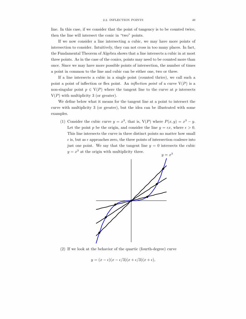
2.2. INFLECTION POINTS 49
line. In this case, if we consider that the point of tangency is to be counted twice,
then the line will intersect the conic in “two” points.
If we now consider a line intersecting a cubic, we may have more points of
intersection to consider. Intuitively, they can not cross in too many places. In fact,
the Fundamental Theorem of Algebra shows that a line intersects a cubic in at most
three points. As in the case of the conics, points may need to be counted more than
once. Since we may have more possible points of intersection, the number of times
a point in common to the line and cubic can be either one, two or three.
If a line intersects a cubic in a single point (counted thrice), we call such a
point a point of inflection or flex point. An inflection point of a curve V(P ) is a
non-singular point p ∈ V(P ) where the tangent line to the curve at p intersects
V(P ) with multiplicity 3 (or greater).
We define below what it means for the tangent line at a point to intersect the
curve with multiplicity 3 (or greater), but the idea can be illustrated with some
examples.
(1) Consider the cubic curve y = x3, that is, V(P ) where P (x, y) = x3 − y.
Let the point p be the origin, and consider the line y = εx, where ε > 0.
This line intersects the curve in three distinct points no matter how small
ε is, but as ε approaches zero, the three points of intersection coalesce into
just one point. We say that the tangent line y = 0 intersects the cubic
y = x3 at the origin with multiplicity three.y = x3
b
b
b
b
b
b
b
(2) If we look at the behavior of the quartic (fourth-degree) curve
y = (x− ε)(x − ε/3)(x+ ε/3)(x+ ε),
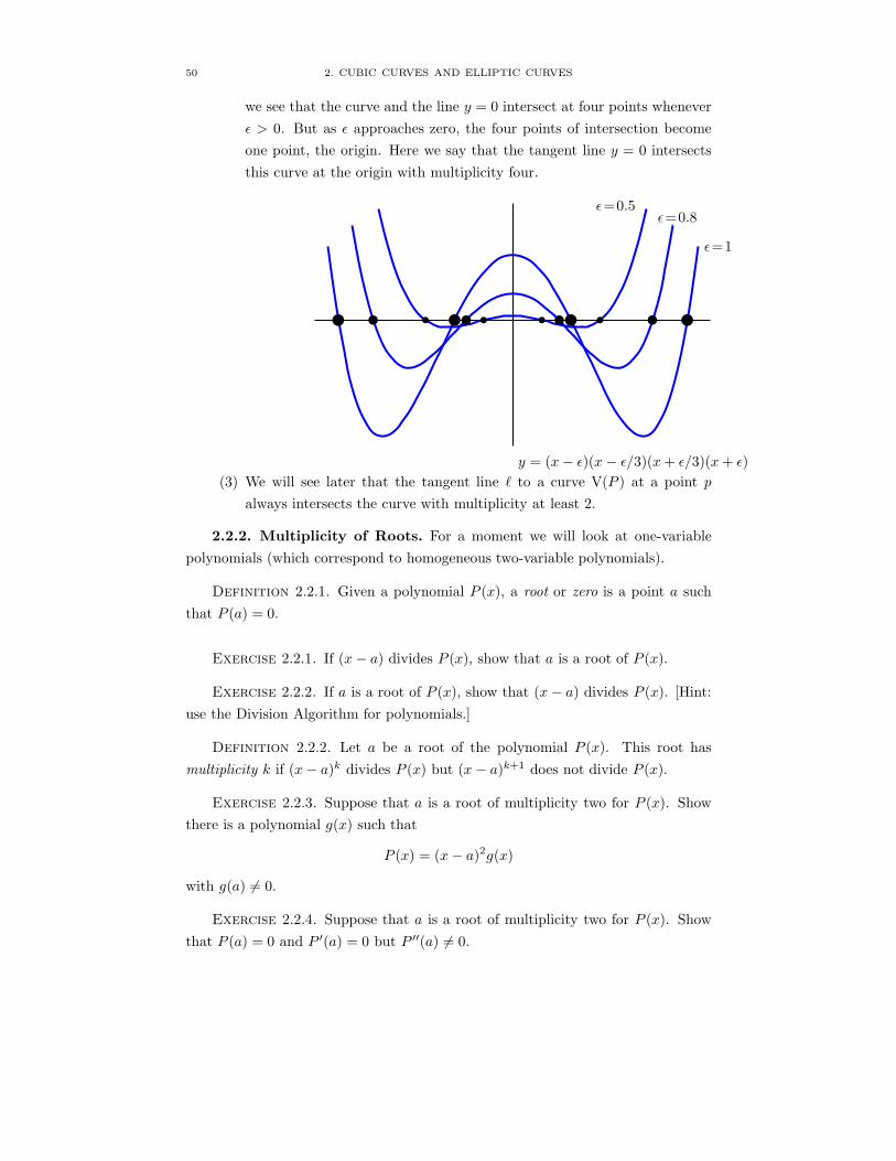
50 2. CUBIC CURVES AND ELLIPTIC CURVES
we see that the curve and the line y = 0 intersect at four points whenever
ε > 0. But as ε approaches zero, the four points of intersection become
one point, the origin. Here we say that the tangent line y = 0 intersects
this curve at the origin with multiplicity four.
b b b bb b b bb b b b
ε=1
ε=0.8ε=0.5
y = (x− ε)(x − ε/3)(x+ ε/3)(x+ ε)
(3) We will see later that the tangent line ` to a curve V(P ) at a point p
always intersects the curve with multiplicity at least 2.
2.2.2. Multiplicity of Roots. For a moment we will look at one-variable
polynomials (which correspond to homogeneous two-variable polynomials).
Definition 2.2.1. Given a polynomial P (x), a root or zero is a point a such
that P (a) = 0.
Exercise 2.2.1. If (x− a) divides P (x), show that a is a root of P (x).
Exercise 2.2.2. If a is a root of P (x), show that (x− a) divides P (x). [Hint:
use the Division Algorithm for polynomials.]
Definition 2.2.2. Let a be a root of the polynomial P (x). This root has
multiplicity k if (x− a)k divides P (x) but (x − a)k+1 does not divide P (x).
Exercise 2.2.3. Suppose that a is a root of multiplicity two for P (x). Show
there is a polynomial g(x) such that
P (x) = (x− a)2g(x)
with g(a) 6= 0.
Exercise 2.2.4. Suppose that a is a root of multiplicity two for P (x). Show
that P (a) = 0 and P ′(a) = 0 but P ′′(a) 6= 0.

2.2. INFLECTION POINTS 51
Exercise 2.2.5. Suppose that a be a root of multiplicity k for P (x). Show
there is a polynomial g(x) such that
P (x) = (x − a)kg(x)
with g(a) 6= 0.
Exercise 2.2.6. Suppose that a is a root of multiplicity k for P (x). Show that
P (a) = P ′(a) = · · · = P (k−1)(a) = 0 but that P (k)(a) 6= 0.
The homogeneous version is the following.
Definition 2.2.3. Let P (x, y) be a homogeneous polynomial. A root or zero
is a point (a : b) ∈ P1 such that P (a, b) = 0. If (a : b) is a root of P (x, y), then
(bx− ay) divides P (x, y). This root has multiplicity k if (bx− ay)k divides P (x, y)
but (bx− ay)k+1 does not divide P (x, y).
Exercise 2.2.7. Suppose that (a : b) is a root of multiplicity two for P (x, y).
Show that
P (a, b) =∂P
∂x(a, b) =
∂P
∂y(a, b) = 0,
but at least one of the second partials does not vanish at (a : b).
Exercise 2.2.8. Suppose that (a : b) is a root of multiplicity k for P (x, y).
Show that
P (a, b) =∂P
∂x(a, b) =
∂P
∂y(a, b) = · · · = ∂k−1P
∂xi∂yj(a, b) = 0,
where i+ j = k − 1 but that
∂kP
∂xi∂yj(a, b) 6= 0,
for at least one pair i + j = k. This means that the first partials, second partials,
etc. up to the k − 1 partials all vanish at (a : b), but that at least one of the kth
partials does not vanish at (a : b).
2.2.3. Inflection Points. Let P (x, y, z) be a homogeneous polynomial. We
want to understand what it means for a line to intersect V(P ) in a point with
multiplicity three or more. Let
l(x, y, z) = ax+ by + cz
be a linear polynomial and let ` = V(l) be the corresponding line in P2. We are
tacitly assuming that not all of a, b, c are zero. We might as well assume that b 6= 0.
That is, by a projective change of coordinates we may assume that b 6= 0. We
can multiply l by any nonzero constant and still have the same line, meaning that
for λ 6= 0, we have V(l) = V(λl). So, we can assume that b = −1. The reason

52 2. CUBIC CURVES AND ELLIPTIC CURVES
for the −1 is that we now know that all points on the line have the property that
y = ax+ cz.
Exercise 2.2.9. Let (x0 : y0 : z0) ∈ V(P )∩V(l). Show that (x0 : z0) is a root of
the homogeneous two-variable polynomial P (x, ax+ cz, z) and that y0 = ax0+ cz0.
Definition 2.2.4. The intersection multiplicity of V(P ) and V(l) at (x0 : y0 :
z0) is the multiplicity of the root (x0 : z0) of P (x, ax+ cz, z).
Exercise 2.2.10. Let P (x, y, z) = x2 − yz and l(x, y, z) = λx − y. Show that
the intersection multiplicity of V(P ) and V(l) at (0 : 0 : 1) is one when λ 6= 0 and
is two when λ = 0.
The key to the definition above is that, when b = −1, the system x = x, y =
ax + cz, z = z gives a parametrization of the line V(l) and the intersection multi-
plicity of V(P ) and V(l) at (x0 : y0 : z0) is found by considering P evaluated as a
function of these two parameters. The next exercise proves the important fact that
the intersection multiplicity is independent of the choice of parametrization of the
line V(l) used.
Exercise 2.2.11. Let (x0 : y0 : z0) ∈ V(P ) ∩ V(l). Let x = a1s + b1t, y =
a2s + b2t, z = a3s + b3t and x = c1u + d1v, y = c2u + d2v, z = c3u + d3v be two
parametrizations of the line V(l) such that (x0 : y0 : z0) corresponds to (s0 : t0)
and (u0 : v0), respectively. Show that the multiplicity of the root (s0 : t0) of
P (a1s + b1t, a2s + b2t, a3s + b3t) is equal to the multiplicity of the root (u0 : v0)
of P (c1u + d1v, y = c2u+ d2v, z = c3u + d3v). Conclude that our definition of the
intersection multiplicity of V(P ) and V(l) is independent of the parametrization of
the line V(l) used.
Exercise 2.2.12. Let P (x, y, z) = x2+2xy−yz+z2. Show that the intersection
multiplicity of V(P ) and any line ` at a point of intersection is at most two.
Exercise 2.2.13. Let P (x, y, z) be an irreducible second degree homogeneous
polynomial. Show that the intersection multiplicity of V(P ) and any line ` at a
point of intersection is at most two.
Exercise 2.2.14. Let P (x, y, z) = x2 + y2 + 2xz − yz.
(1) Find the tangent line ` = V(l) to V(P ) at (−2 : 1 : 1).
(2) Show that the intersection multiplicity of V(P ) and ` at (−2 : 1 : 1) is
two.
Exercise 2.2.15. Let P (x, y, z) = x3 − y2z + z3.
(1) Find the tangent line to V(P ) at (2 : 3 : 1) and show directly that the
intersection multiplicity of V(P ) and its tangent at (2 : 3 : 1) is two.

2.2. INFLECTION POINTS 53
(2) Find the tangent line to V(P ) at (0 : 1 : 1) and show directly that the
intersection multiplicity of V(P ) and its tangent at (0 : 1 : 1) is three.
Exercise 2.2.16. Redo the previous two exercises using Exercise 2.2.8.
Exercise 2.2.17. Show that for any non-singular curve V(P ) ⊂ P2, the inter-
section multiplicity of V(P ) and its tangent line ` at the point of tangency is at
least two.
Exercise 2.2.18.
(1) Let P (x, y, z) be an irreducible degree three homogeneous polynomial.
Show that the intersection multiplicity of V(P ) and any line ` at a point
of intersection is at most three.
(2) Let P (x, y, z) be an irreducible homogeneous polynomial of degree n.
Show that the intersection multiplicity of V(P ) and any line ` at a point
of intersection is at most n.
Definition 2.2.5. Let P (x, y, z) be an irreducible homogeneous polynomial of
degree n. A non-singular point p ∈ V(P ) ⊂ P2 is called a point of inflection or a
flex of the curve V(P ) if the tangent line to the curve at p intersects V(P ) with
multiplicity at least three.
Exercise 2.2.19. Let P (x, y, z) = x3+yz2. Show that (0 : 0 : 1) is an inflection
point of V(P ).
Exercise 2.2.20. Let P (x, y, z) = x3 + y3 + z3 (the Fermat curve). Show that
(1 : −1 : 0) is an inflection point of V (P ).
2.2.4. Hessians. We have just defined what it means for a point p ∈ V(P )
to be a point of inflection. Checking to see whether a given point p ∈ V(P ) is
an inflection point can be tedious, but finding inflection points can be extremely
difficult task with our current tools. How did we know to check (1 : −1 : 0) in
Exercise 2.2.20? As we know V(P ) has an infinite number of points, so it would
be impossible to find the tangent at every point and to check the intersection
multiplicity. Moreover, if these inflection points are related to the inflection points
of calculus, where are the second derivatives? The Hessian curve will completely
solve these difficulties. We will first define the Hessian curve, then determine how
it can be used to find the points of inflection.
Definition 2.2.6. Let P (x, y, z) be a homogeneous polynomial of degree n.
The Hessian H(P ) is
H(P )(x, y, z) = det
Pxx Pxy Pxz
Pxy Pyy Pyz
Pxz Pyz Pzz
,

54 2. CUBIC CURVES AND ELLIPTIC CURVES
where
Px =∂P
∂x
Pxx =∂2P
∂x2
Pxy =∂2P
∂x∂y, etc.
The Hessian curve is V(H(P )).
Exercise 2.2.21. Compute H(P ) for the following cubic polynomials.
(1) P (x, y, z) = x3 + yz2
(2) P (x, y, z) = y3 + z3 + xy2 − 3yz2 + 3zy2
(3) P (x, y, z) = x3 + y3 + z3
Exercise 2.2.22. Let P (x, y, z) be an irreducible homogeneous polynomial of
degree three. Show that H(P ) is also a third degree homogeneous polynomial.
We want to link the Hessian curve with inflection points.
Exercise 2.2.23. Let P (x, y, z) = x3 + y3 + z3 (the Fermat curve). Show that
(1 : −1 : 0) ∈ V(P ) ∩ V(H(P )).
Exercise 2.2.24. Let P (x, y, z) = y3 + z3 + xy2 − 3yz2 + 3zy2. Show that
(−2 : 1 : 1) ∈ V(P ) ∩ V(H(P )).
Exercise 2.2.25. Let P (x, y, z) = x3 + yz2. Show that (0 : 0 : 1) ∈ V(P ) ∩V(H(P )).
These exercises suggest a link between inflection points of V(P ) and points in
V(P ) ∩ V(H(P )), but we need to be careful.
Exercise 2.2.26. Let P (x, y, z) = x3 + yz2.
(1) Show that (0 : 1 : 0) ∈ V(P ) ∩ V(H(P )).
(2) Explain why (0 : 1 : 0) is not an inflection point of V(P ).
We can now state the relationship we want.
Theorem 2.2.27. Let P (x, y, z) be a homogeneous polynomial of degree d. If
V(P ) is smooth, then p ∈ V(P ) ∩ V(H(P )) if and only if p is a point of inflection
of V(P ).
We will prove this theorem through a series of exercises.1 The first thing we
need to show is that the vanishing of the Hessian V(H(P )) is invariant under a
projective change of coordinates.
1The following exercises are based on the proof taken from C. G. Gibson’s “Elementary
Geometry of Algebraic Curves.”[Gib98]

2.2. INFLECTION POINTS 55
Exercise 2.2.28. Consider the following projective change of coordinatesu
v
w
= A
x
y
z
,
where
A =
a11 a12 a13
a21 a22 a23
a31 a32 a33
.
Suppose that under the projective transformation A the polynomial P (x, y, z) be-
comes the polynomial Q(u, v, w).
(1) Show that the Hessian matrices of P and Q are related byPxx Pxy Pxz
Pxy Pyy Pyz
Pxz Pyz Pzz
= AT
Quu Quv Quw
Quv Qvv Qvw
Quw Qvw Qww
A.
(2) Conclude that H(P )(x, y, z) = 0 if and only if H(Q)(u, v, w) = 0.
Next we need to show that inflection points are mapped to inflection points
under a projective change of coordinates.
Exercise 2.2.29. Suppose p is a point of inflection of V(P ), and that under a
projective change of coordinates the polynomial P becomes the polynomial Q and
p 7→ q. Show that q is a point of inflection of V(Q).
In the next exercise, we will reduce the proof of Theorem 2.2.27 to the case
where p = (0 : 0 : 1) ∈ V(P ) and the tangent line to V(P ) at p is ` = V(y).
Exercise 2.2.30. Use Exercises 2.2.28 and 2.2.29 to explain why to prove
Theorem 2.2.27 it is enough to show that p is a point of inflection if and only if
H(P )(p) = 0 in the case where p = (0 : 0 : 1) ∈ V(P ) and the tangent line ` to
V(P ) at p is y = 0, i.e. ` = V(y).
Thus we will assume that the point p = (0 : 0 : 1) ∈ V(P ) and that the tangent
line to V(P ) at p is y = 0 from now until the end of Exercise 2.2.34.
Exercise 2.2.31. Explain why in the affine patch z = 1 the dehomogenized
curve is
λy + (ax2 + bxy + cy2) + higher order terms,
where λ 6= 0. [Hint: We know that p ∈ V(P ) and p is non-singular.]
From this we can conclude that P (x, y, z) is given by
(2.1) P (x, y, z) = λyzd−1 + (ax2 + bxy + cy2)zd−2 + higher order terms
where d = degP .

56 2. CUBIC CURVES AND ELLIPTIC CURVES
Exercise 2.2.32. Explain why the intersection of V(P ) with the tangent V(y)
at p corresponds to the root (0 : 1) of the equation
P (x, 0, z) = ax2zd−2 + higher order terms = 0.
Exercise 2.2.33. Show that p is a point of inflection of V(P ) if and only if
a = 0. [Hint: For p to be an inflection point, what must the multiplicity of (0 : 1)
be in the equation in Exercise 2.2.32?]
We have now established that p is a point of inflection if and only if a = 0 in
Equation (2.1). All that remains is to show that p ∈ V(H(P )) if and only if a = 0.
Exercise 2.2.34.
(1) Show that
H(P )(p) = det
2a b 0
b 2c λ(d− 1)
0 λ(d− 1) 0
.
(2) Conclude that p ∈ V(H(P )) if and only if a = 0.
This completes our proof of Theorem 2.2.27. In practice, we use the Hessian
to locate inflection points even if V(P ) is not smooth by finding the points of
intersection of V(P ) and V(H(P )) and eliminating those that are singular on V(P ).
Exercise 2.2.35. Let P (x, y, z) be an irreducible second degree homogeneous
polynomial. Using the Hessian curve, show that V(P ) has no points of inflection.
We conclude this section with the following theorem, which we state without
proof. Theorem 2.2.36 is a direct result of Bezout’s theorem, which we will prove
in Section 3.3.27.
Theorem 2.2.36. Two cubic curves in P2 will intersect in exactly 3 × 3 = 9
points, counted up to intersection multiplicities.
Exercise 2.2.37. Use Exercise 2.2.22 and Theorem 2.2.27 to show that if V(P )
is a smooth cubic curve, then V(P ) has exactly nine inflection points.
Exercise 2.2.38. Find all nine points of inflection of the Fermat curve, P (x, y, z) =
x3 + y3 + z3.
2.3. Group Law
The goal of this section is to illustrate that, as a consequence of their geometric
structure, smooth cubic curves are abelian groups. While the group law can be
stated algebraically, in this section we will develop it geometrically to see why it is
important for the curve to have degree three.

2.3. GROUP LAW 57
2.3.1. Adding points on smooth cubics. Let C denote a smooth cubic
curve in the projective plane, P2(C). We will develop a geometric method for
adding points so that C is an abelian group under this operation. First, we define
an abelian group.
Definition 2.3.1. A group is a set G equipped with a binary operation ?
satisfying the following axioms:
(G1) The binary operation is associative, i.e.,
g1 ? (g2 ? g3) = (g1 ? g2) ? g3
for all g1, g2, g3 ∈ G.
(G2) There is an (unique) identity element e ∈ G such that e ? g = g = g ? e for
all g ∈ G.
(G3) For each g ∈ G, there is an (unique) inverse element g′ ∈ G satisfying
g ? g′ = e = g′ ? g.
A group G is said to be an abelian group if, in addition, the binary operation
? is commutative, i.e., g1 ? g2 = g2 ? g1 for all g1, g2 ∈ G.
For points P and Q on C, let `(P,Q) denote the line in P2 through P and Q. In
case P and Q are the same point, let `(P, P ) be the line tangent to C at P . (This is
why we must assume the cubic curve C is smooth, in order to ensure there is a well-
defined tangent line at every point.) In Section 2.2.3 we saw that the Fundamental
Theorem of Algebra ensures there are exactly three points of intersection of `(P,Q)
with the cubic curve C, counting multiplicities. Let PQ denote this unique third
point of intersection, so that the three points of intersection of C with `(P,Q) are
P , Q and PQ. In the event that a line ` is tangent to C at P , then the multiplicity
of P is at least two by Exercise 2.2.17. Therefore, if P 6= Q and `(P,Q) is tangent
to C at P , then PQ = P , for P counted the second time is the third point of
intersection of `(P,Q) with C. The rule (P,Q) 7→ PQ gives a binary operation on
C, which is called the chord-tangent composition law .
Exercise 2.3.1. Explain why the chord-tangent composition law is commuta-
tive, i.e., PQ = QP for all points P,Q on C.
While this is a well-defined, commutative binary operation on C, the following
exercises illustrate that the chord-tangent composition law lacks the properties
required of a group law.
Exercise 2.3.2. Consider the cubic curve C = (x, y) ∈ C2 | y2 = x3 − xand the points P,Q,R on C, as shown below. (Note that only the real part of C is
shown.)
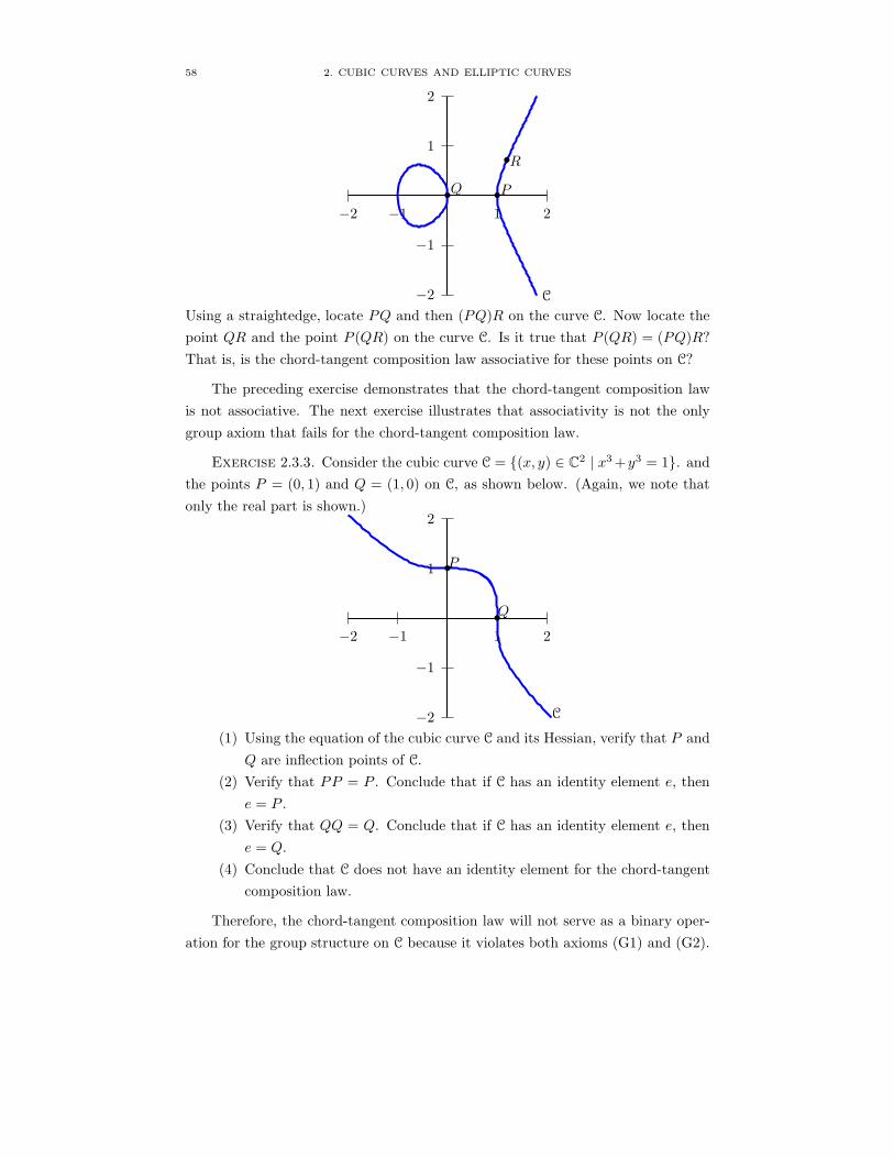
58 2. CUBIC CURVES AND ELLIPTIC CURVES
1
2
−1
−2
1 2−1−2
C
•P•Q
•R
Using a straightedge, locate PQ and then (PQ)R on the curve C. Now locate the
point QR and the point P (QR) on the curve C. Is it true that P (QR) = (PQ)R?
That is, is the chord-tangent composition law associative for these points on C?
The preceding exercise demonstrates that the chord-tangent composition law
is not associative. The next exercise illustrates that associativity is not the only
group axiom that fails for the chord-tangent composition law.
Exercise 2.3.3. Consider the cubic curve C = (x, y) ∈ C2 | x3+y3 = 1. andthe points P = (0, 1) and Q = (1, 0) on C, as shown below. (Again, we note that
only the real part is shown.)
1
2
−1
−2
1 2−1−2
C
•P
•Q
(1) Using the equation of the cubic curve C and its Hessian, verify that P and
Q are inflection points of C.
(2) Verify that PP = P . Conclude that if C has an identity element e, then
e = P .
(3) Verify that QQ = Q. Conclude that if C has an identity element e, then
e = Q.
(4) Conclude that C does not have an identity element for the chord-tangent
composition law.
Therefore, the chord-tangent composition law will not serve as a binary oper-
ation for the group structure on C because it violates both axioms (G1) and (G2).

2.3. GROUP LAW 59
However, we can find a way to make this work. By using the chord-tangent com-
position law twice in combination with a fixed inflection point, we will construct
the group law on C in the next subsection.
2.3.2. Group Law with an Inflection Point. Let C denote a smooth cubic
curve in the projective plane, P2(C). As we showed in Exercise 2.2.37 , there
are nine points of inflection (counting multiplicity) on C. These are the points of
intersection of the cubic curve, C, with its Hessian curve.
Select a point of inflection O on C. We define our binary operation, +, relative
to this specific point O. For points P,Q on C, define P +Q to be the unique third
point of intersection of `(O,PQ) with C, where PQ denotes the chord-tangent
composition of P and Q. That is, P + Q = O(PQ), using the chord-tangent
composition law notation. We claim that with this binary operation +, C is an
abelian group, and we call this operation addition, i.e. we can “add” points on C.
We will prove that for a given choice of inflection point, O, the cubic curve
C with addition of points relative to O is an abelian group. Before we verify this
claim, let’s consider a specific example.
1
2
3
4
−1
−2
−3
−4
1 2 3−1−2
C
•P1
•P2
•P3
•P4
•P5
Figure 1. The cubic curve C = V (x3 − y2z + z3) in the affine
patch z = 1

60 2. CUBIC CURVES AND ELLIPTIC CURVES
Consider the cubic curve C = V (x3 − y2z + z3) ⊂ P2, and the points P1 = (2 :
3 : 1), P2 = (0 : 1 : 1), P3 = (−1 : 0 : 1), P4 = (0 : −1 : 1), P5 = (2 : −3 : 1) on C.
Figure 2.3.2 shows C in the affine patch z = 1.
Exercise 2.3.4. Use the equations of the cubic curve C and its Hessian to
verify that P2 and P4 are inflection points of C.
Exercise 2.3.5. Let O = P2 be the specified inflection point so that + is
defined relative to P2, i.e. Q+R = P2(QR) for points Q,R on C.
(1) Compute P1 + P2, P2 + P2, P3 + P2, P4 + P2, and P5 + P2.
(2) Explain why P2 is the identity element for C.
(3) Find the inverses of P1, P2, P3, P4 and P5 on C.
(4) Verify that P1+(P3+P4) = (P1+P3)+P4. In general, addition of points
on C is associative.
Exercise 2.3.6. Now let O = P4 be the specified inflection point so that + is
defined relative to P4, i.e. Q+R = P4(QR) for points Q,R on C.
(1) Compute P1 + P2, P2 + P2, P3 + P2, P4 + P2, and P5 + P2. [Hint: For
P4+P2 and P5+P2 find the equations of the lines `(P4, P2) and `(P5, P2),
respectively, to find the third points of intersection with C.] Are the
answers the same as they were in part (1) of Exercise 2.3.5? Is P2 still
the identity element for C?
(2) Now compute P1 + P4, P2 + P4, P3 + P4, P4 + P4, and P5 + P4. Explain
why P4 is now the identity element for C.
(3) Using the fact that P4 is now the identity element on C, find the inverses
of P1, P2, P3, P4 and P5 on C. [Hint: See the hint on part (1).] Are these
the same as the inverses found in part (3) of Exercise 2.3.5?
Now we will prove that the cubic curve C with addition of points relative to
a fixed inflection point O is an abelian group. First, we verify that the binary
operation + is commutative.
Exercise 2.3.7. Explain why P + Q = Q + P for all points P,Q on C. This
establishes that + is a commutative binary operation on C.
In Exercises 2.3.5 and 2.3.6, the inflection point used to define the addition also
served as the identity element for the curve C = V (x3 − y2z + z3). In the exercise
below, you will show this is true for any cubic curve.
Exercise 2.3.8. Let C be a smooth cubic curve and let O be one of its inflection
points. Define addition, +, of points on C relative to O. Show that P +O = P for
all points P on C and that there is no other point on C with this property. Thus O
is the identity element for + on C.
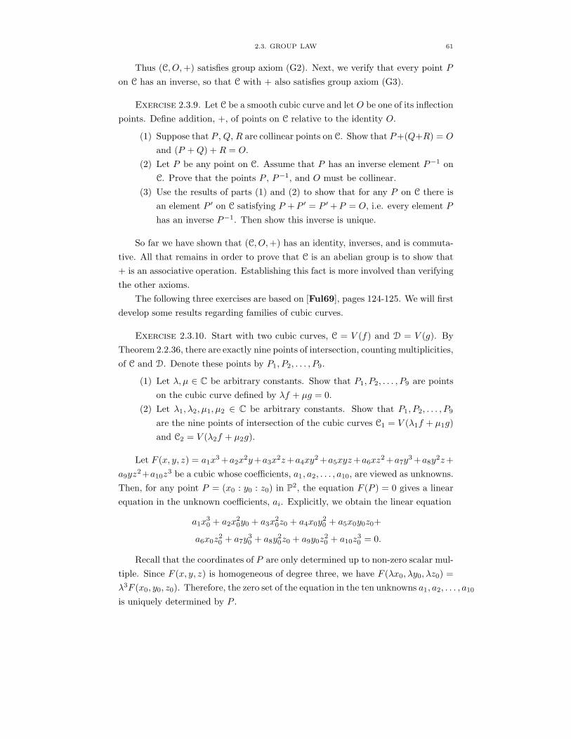
2.3. GROUP LAW 61
Thus (C, O,+) satisfies group axiom (G2). Next, we verify that every point P
on C has an inverse, so that C with + also satisfies group axiom (G3).
Exercise 2.3.9. Let C be a smooth cubic curve and let O be one of its inflection
points. Define addition, +, of points on C relative to the identity O.
(1) Suppose that P , Q, R are collinear points on C. Show that P+(Q+R) = O
and (P +Q) +R = O.
(2) Let P be any point on C. Assume that P has an inverse element P−1 on
C. Prove that the points P , P−1, and O must be collinear.
(3) Use the results of parts (1) and (2) to show that for any P on C there is
an element P ′ on C satisfying P +P ′ = P ′ +P = O, i.e. every element P
has an inverse P−1. Then show this inverse is unique.
So far we have shown that (C, O,+) has an identity, inverses, and is commuta-
tive. All that remains in order to prove that C is an abelian group is to show that
+ is an associative operation. Establishing this fact is more involved than verifying
the other axioms.
The following three exercises are based on [Ful69], pages 124-125. We will first
develop some results regarding families of cubic curves.
Exercise 2.3.10. Start with two cubic curves, C = V (f) and D = V (g). By
Theorem 2.2.36, there are exactly nine points of intersection, counting multiplicities,
of C and D. Denote these points by P1, P2, . . . , P9.
(1) Let λ, µ ∈ C be arbitrary constants. Show that P1, P2, . . . , P9 are points
on the cubic curve defined by λf + µg = 0.
(2) Let λ1, λ2, µ1, µ2 ∈ C be arbitrary constants. Show that P1, P2, . . . , P9
are the nine points of intersection of the cubic curves C1 = V (λ1f + µ1g)
and C2 = V (λ2f + µ2g).
Let F (x, y, z) = a1x3+a2x
2y+a3x2z+a4xy
2+a5xyz+a6xz2+a7y
3+a8y2z+
a9yz2+a10z
3 be a cubic whose coefficients, a1, a2, . . . , a10, are viewed as unknowns.
Then, for any point P = (x0 : y0 : z0) in P2, the equation F (P ) = 0 gives a linear
equation in the unknown coefficients, ai. Explicitly, we obtain the linear equation
a1x30 + a2x
20y0 + a3x
20z0 + a4x0y
20 + a5x0y0z0+
a6x0z20 + a7y
30 + a8y
20z0 + a9y0z
20 + a10z
30 = 0.
Recall that the coordinates of P are only determined up to non-zero scalar mul-
tiple. Since F (x, y, z) is homogeneous of degree three, we have F (λx0, λy0, λz0) =
λ3F (x0, y0, z0). Therefore, the zero set of the equation in the ten unknowns a1, a2, . . . , a10
is uniquely determined by P .
62 2. CUBIC CURVES AND ELLIPTIC CURVES
Exercise 2.3.11. Consider eight distinct points in P2, say P1, P2, . . . , P8, that
are in general position, which for us means that no four are collinear and no seven
are on a single conic. Let F be a generic cubic polynomial with unknown coefficients
a1, a2, . . . , a10. The system of simultaneous equations F (P1) = F (P2) = · · · =
F (P8) = 0 is a system of eight linear equations in the ten unknowns a1, a2, . . . , a10.
(1) Show that if the eight points P1, P2, . . . , P8 are in general position, then
the rank of the linear system F (P1) = F (P2) = · · · = F (P8) = 0 is equal
to 8.
(2) Use the Rank-Nullity theorem from linear algebra to show that there are
two “linearly independent” cubics F1(x, y, z) and F2(x, y, z) such that any
cubic curve passing through the eight points P1, P2, . . . , P8 has the form
λF1 + µF2.
(3) Conclude that for any collection of eight points in general position, there
is a unique ninth point P9 such that every cubic curve passing through
the eight given points must also pass through P9.
In this next exercise, we prove the associativity of the newly defined addition
of points on a smooth cubic curve.
Exercise 2.3.12. Let C be a smooth cubic curve in P2 and let P,Q,R be three
points on C. We will show that P + (Q+ R) = (P +Q) +R.
• Let V (l1) = `(P,Q) and S1 = PQ, so V (l1) ∩ C = P,Q, S1.• Let V (l2) = `(S1, O) and S2 = OS1 = P +Q, so V (l2) ∩ C = S1, O, S2.• Let V (l3) = `(S2, R) and S3 = (P +Q)R, so V (l3) ∩ C = S2, R, S3.
Similarly,
• Let V (m1) = `(Q,R) and T1 = QR, so V (m1) ∩ C = Q,R, T1.• Let V (m2) = `(T1, O) and T2 = OT1 = Q+R, so V (m2)∩C = T1, O, T2.• Let V (m3) = `(T2, P ) and T3 = P (Q +R), so V (m3) ∩ C = T2, P, T3.
(1) Notice that C′ = V (l1m2l3) is a cubic. Find C′ ∩ C.
(2) Likewise, C′′ = V (m1l2m3) is a cubic. Find C′′ ∩ C.
(3) Using parts (1) and (2) together with Exercise 2.3.11, deduce that (P +
Q)R = P (Q +R).
(4) Explain why (P+Q)R = P (Q+R) implies that (P+Q)+R = P+(Q+R).
Conclude that the addition of points on cubics is associative.
Therefore, a cubic curve C with a selected inflection pointO determines a binary
operation, +, in such a way that (C, O,+) is an abelian group under addition.2
2We defined addition on C relative to an inflection point, O, but we could define addition on
C relative to any point O on C. See Husemoller, “Elliptic Curves”, Theorem 1.2 for details.

2.3. GROUP LAW 63
Since (C, O,+) is a group, it is natural to ask group theoretic questions about
C, such as questions regarding the orders of its elements. First we define an integer
multiple of a point and the order of a point.
Definition 2.3.2. Let (C, O,+) be a smooth cubic curve and let P 6= O be a
point on the curve. For n ∈ Z we define n · P as follows:
• 0 · P = O and 1 · P = P
• For n ≥ 2, we have n · P = (n− 1)P + P
• For n < 0, we set n · P to be the inverse of −n · P .
Definition 2.3.3. Let (C, O,+) be a smooth cubic curve and let P 6= O be a
point on the curve. If there exists a positive integer n so that n · P = O and for
1 ≤ m ≤ n−1 we have m ·P 6= O, then the point P has order n. If no such positive
integer exists, then the point is said to have infinite order.
We can now examine points of finite order. In particular, we are interested here
in points of order two and three. Many areas of mathematics are concerned with
the computation of the order of various points on a cubic curve.
2.3.3. Points of Order Two and Three. Let C be a smooth cubic curve
with + defined relative to the inflection point O, the group identity. Let P be a
point on C.
Exercise 2.3.13. Show that 2P = O if and only if `(O,P ) is tangent to C at
P .
Exercise 2.3.14. Show that if P and Q are two points on C of order two, then
PQ, the third point of intersection of C with `(P,Q), is also a point of order two
on C.
Exercise 2.3.15. Let C be the cubic curve defined by y2z = x3 − xz2. Graph
C in the affine patch z = 1, and find three points of order two.
Let C be a smooth cubic curve with + defined relative to the inflection point
O.
Exercise 2.3.16. Let P be any inflection point on C. Show that 3P = O.
Exercise 2.3.17. Suppose P is point on C and 3P = O. Conclude that PP =
P . From this, deduce that P is a point of inflection on C.
We will return to points of finite order in section 2.4.3 after we have developed
a more convenient way to express our smooth cubic curves.
64 2. CUBIC CURVES AND ELLIPTIC CURVES
2.4. Normal forms of cubics
The goal of this section3 is to show that every smooth cubic is projectively equiv-
alent to one of the form y2 = x3 + Ax + B, the Weierstrass normal form, where
the coefficients A and B are determined uniquely. See Equation (2.7). We will
also show that every smooth cubic is projectively equivalent to the canonical form
y2 = x(x−1)(x−λ). See Equation 2.4.24. The value of λ, however, is not uniquely
determined, as there are six values of λ for the same cubic. We associate to each
cubic a complex number and vice versa showing that we can parametrize all cubics
by the complex numbers. Using this, in the next section we will give an algebraic
characterization of the group law, which may then be used not only in characteristic
zero, but for positive characteristics and even over non-algebraically closed fields
such as R, Q, and Zp.
2.4.1. Weierstrass Normal Form. One set of problems will be to achieve
the goals outlined above for a general cubic curve C. The other set of problems
consists of carrying out the computations with a concrete example, the curve x3+y3 − z3 = 0.
Let C be a smooth cubic curve in P2 given by the homogeneous equation
f(x, y, z) = 0. Select an inflection point, O = (a0 : b0 : c0), on C and let ` denote
the tangent line to C at O, where ` is defined by the linear equation l(x,y,z)=0.
Recall that we can projectively change coordinates with an invertible 3× 3 matrix
M . x1
y1
z1
=M
x
y
z
.
We choose M so that 0
1
0
=M
a0
b0
c0
and ` is transformed to the line defined by l1(x1, y1, z1) = z1, i.e. the inflection
point O becomes and (0 : 1 : 0) and the tangent line ` becomes the line z1 = 0under the projective change of coordinates M . Recall, that we actually carry out
the computations of changing coordinates by using the inverse M−1 of M and
replacing x, y, and z with expressions involving x1, y1, and z1.
Exercise 2.4.1. Consider the smooth cubic curve C defined by x3+y3−z3 = 0.
(1) Show that O = (1 : 0 : 1) is an inflection point of C.
3The development in this section follows the first two sections of chapter three of J. Silver-
man’s The Arithmetic of Elliptic Curves.

2.4. NORMAL FORMS OF CUBICS 65
(2) Show that x− z = 0 is the equation of the tangent line to C at O.
(3) Find a 3× 3 matrix M such that, under the change of variablesx
y
z
=M−1
x1
y1
z1
,
we have (1 : 0 : 1) 7→ (0 : 1 : 0) and l(x, y, z) = x − z becomes
l1(x1, y1, z1) = z1.
(4) Find the equation, f1(x1, y1, z1) = 0, for the curve C1 that is associated
to this projective change of coordinates.
Now we have transformed our original smooth cubic curve C into another
smooth cubic curve C1, which is projectively equivalent to C. Let’s now work
with the new curve C1 that is defined by the equation f1(x1, y1, z1) = 0 in P2 with
coordinates (x1 : y1 : z1).
Exercise 2.4.2.
(1) Explain why the homogeneous polynomial f1(x1, y1, z1) can be expressed
as
f1(x1, y1, z1) = αx31 + z1F (x1, y1, z1),
where α 6= 0 and F (0, 1, 0) 6= 0.
(2) Explain why the highest power of y1 in the homogeneous polynomial
f1(x1, y1, z1) is two.
(3) Explain how by rescaling we can introduce new coordinates (x2 : y2 : z2)
so that the coefficient of x32 is 1 and the coefficient of y22z2 is −1 in the
new homogeneous polynomial f2(x2, y2, z2) = 0.
We can now rearrange the equation f2(x2, y2, z2) = 0 to be of the form
(2.2) y22z2 + a1x2y2z2 + a3y2z22 = x32 + a2x
22z2 + a4x2z
22 + a6z
32 .
Exercise 2.4.3. Refer to the curve defined in Exercise 2.4.1 for the following.
(1) Show that the matrix
M−1 =
0 1 0
1 0 1
0 1 −1
does what we want for part (3) of Exercise 2.4.1.
(2) Find the homogeneous polynomial f1(x1, y1, z1) that corresponds to this
projective change of coordinates.
(3) Verify that f1 is of the form f1(x1, y1, z1) = αx31 + z1F (x1, y1, z1), where
α 6= 0 and F (0, 1, 0) 6= 0.

66 2. CUBIC CURVES AND ELLIPTIC CURVES
(4) Rescale, if necessary, so that the coefficient of x2 is 1 and the coefficient
of y22z2 is −1.
(5) Rearrange f2(x2, y2, z2) = 0 to be in the form of equation (2.2).
Let’s now work in the affine patch z2 = 1, that is, in the affine (x2, y2) plane,
and consider the nonhomogeneous form of equation (2.2),
(2.3) y22 + a1x2y2 + a3y2 = x32 + a2x22 + a4x2 + a6,
keeping in mind that there is an extra point at infinity. We can treat the left-hand
side of equation (2.3) as a quadratic expression in y2. This means we can complete
the square to remove some of the terms.
Consider the following concrete examples.
Exercise 2.4.4.
(1) Complete the square on the left hand side of the following equation.
y2 + 2y = 8x3 + x− 1
(2) Find an affine change of coordinates so that y2+2y = 8x3+x−1 becomes
v2 = f(u).
Exercise 2.4.5.
(1) Complete the square (with respect to y) on the left hand side of the
following equation.
y2 + 4xy + 2y = x3 + x− 3
(2) Find an affine change of coordinates such that y2 + 2y = 8x3 + x − 1
becomes v2 = f(u).
Now we can do this in general.
Exercise 2.4.6. Complete the square on the left-hand side of equation (2.3)
and verify that the affine change of coordinates
x3 = x2
y3 = a1x2 + 2y2 + a3
gives the new equation
(2.4) y23 = 4x33 + (a21 + 4a2)x23 + 2(a1a3 + 2a4)x3 + (a23 + 4a6)
To simplify notation, we introduce the following.
b2 = a21 + 4a2
b4 = a1a3 + 2a4
b6 = a23 + 4a6
2.4. NORMAL FORMS OF CUBICS 67
so that equation (2.4) becomes
(2.5) y23 = 4x33 + b2x23 + 2b4x3 + b6.
We are now ready to make the final affine change of coordinates to achieve
the Weierstrass normal form. Our goal is to scale the coefficient of x33 to 1 and to
eliminate the x23 term. 4
Consider the following concrete examples.
Exercise 2.4.7.
(1) Suppose we have the equation
y2 = x3 + 6x2 − 2x+ 5.
Show that the affine change of coordinates
u = x+ 2
v = y
eliminates the quadratic term on the right hand side.
(2) Suppose we have the equation
y2 = 4x3 + 12x2 + 4x− 6.
Show that the affine change of coordinates
u = 36x+ 36
v = 108y
eliminates the quadratic term and rescales the coefficient of the cubic term
to one on the right hand side.
Exercise 2.4.8. Verify that the affine change of coordinates
u = 36x3 + 3b2
v = 108y3
gives the Weierstrass normal form
v2 = u3 − 27(b22 − 24b4)u− 54(b32 + 36b2b4 − 216b6).
4This change of coordinates is similar to completion of the square, but with cubics. This was
first used by Cardano in Ars Magna (in 1545) to achieve a general solution to the cubic equation
x3+αx2+βx+γ = 0. He needed to eliminate the x2 term then, as we do now. Since the coefficient
of the cubic term inhis equation is already one, he simply made the substitution u = x− α/3.

68 2. CUBIC CURVES AND ELLIPTIC CURVES
Again we can introduce the following to simplify notation.
c4 = b22 − 24b4
c6 = −b32 + 36b2b4 − 216b6.
Then we have the following for our Weierstrass normal form.
(2.6) v2 = u3 − 27c4u− 54c6
Let’s collect all of the coefficient substitutions that we have made. Recall that
the ai’s are the coefficients from equation (2.3). Then we have the following.
b2 = a21 + 4a2
b4 = 2a4 + a1a3
b6 = a23 + 4a6
c4 = b22 − 24b4
c6 = −b32 + 36b2b4 − 216b6.
For upcoming computations it is convenient to introduce the following as well.
b8 = a21a6 + 4a2a6 − a1a3a4 + a2a23 − a24
∆ = −b22b8 − 8b34 − 27b26 + 9b2b4b6
j =c34∆
Exercise 2.4.9. Show the following relationships hold.
(1) 4b8 = b2b6 − b24
(2) 1728∆ = c34 − c26
(3) j =1728c34c34 − c26
These are simply brute-force computations.
∆ is called the discriminant of the cubic curve. The discriminant of a poly-
nomial is an expression in the coefficients of a polynomial which is zero if and
only if the polynomial has a multiple root. For example, the quadratic equation
ax2+ bx+ c = 0 has a multiple root if and only if b2− 4ac = 0. Similarly, the cubic
equation αx3 + βx2 + γx+ δ = 0 has a multiple root if and only if
β2γ2 − 4αγ3 − 4β3δ − 27α2δ2 + 18αβγδ = 0.
The discriminant ∆ given above is the discriminant (up to a factor of 16) of the
right hand side cubic in equation (2.5). The number j defined above is called the
j-invariant of the cubic curve. We will see its significance soon.
2.4. NORMAL FORMS OF CUBICS 69
Exercise 2.4.10. Follow the procedure outlined above to write the following
cubics in Weierstrass normal form and use part (3) of Exercise 2.4.9 to calculate
their j- invariants.
(1) y2 + 2y = 8x3 + x− 1
(2) y2 + 4xy + 2y = x3 + x− 3
To avoid even more cumbersome notation, let’s “reset” our variables. Consider
the Weierstrass normal form of a smooth cubic C:
(2.7) y2 = x3 − 27c4x− 54c6
Notice that with the specific example x3 + y3 − z3 = 0 in P2 in exercises 2.4.1
and 2.4.3, we chose the initial change of coordinates, the transformationM , so that
the inflection point is (0 : 1 : 0) with tangent line given by z = 0, but this is not
a unique transformation. Suppose we had chosen a different transformation. That
is, suppose instead of having the equation
y2 + a1xy + a3y = x3 + a2x2 + a4x+ a6
we obtained the equation
y2 + a′1xy + a′3y = x3 + a′2x2 + a′4x+ a′6.
How different would our Weierstrass normal form have been?
Exercise 2.4.11. Show that the only (affine) transformation that takes
y2 + a1xy + a3y = x3 + a2x2 + a4x+ a6
to
v2 + a′1uv + a′3v = u3 + a′2u2 + a′4u+ a′6
is given by
x = α2u+ r
y = α2su+ α3v + t,
with α, r, s, t ∈ C and α 6= 0. [Hint: Start with the projective transformation,
which is also affine,
x = a11u+ a12v + a13w
y = a21u+ a22v + a23w
z = w
and show that the only way to satisfy the condition in this exercise is for the specific
aij to have the form above.]

70 2. CUBIC CURVES AND ELLIPTIC CURVES
Using this change of coordinates, we can compute the following relationships5
between equivalent cubic curves with coefficients ai in equation (2.2) with coordi-
nates (x : y : z) and coefficients a′i with coordinates (u : v : w).
αa′1 = a1 + 2s
α2a′2 = a2 − sa1 + 3r − s2
α3a′3 = a3 + ra1 + 2t
α4a′4 = a4 − sa3 + 2ra2 − (t+ rs)a1 + 3r2 − 2st
α6a′6 = a6 + ra4 − ta3 + r2a2 − rta1 + r3 − t2
α2b′2 = b2 + 12r
α4b′4 = b4 + rb2 + 6r2
α6b′6 = b6 + 2rb4 + r2b2 + 4r3
α6b′8 = b8 + 3rb6 + 3r2b4 + r3b2 + 3r4
α4c′4 = c4
α6c′6 = c6
α12∆′ = ∆
j′ = j
Notice that if two smooth cubic plane curves are projectively equivalent, then
the value j for each is the same, which is why we call this number the j-invariant.
Let C and C′ be two cubic plane curves, written in Weierstrass normal form.
C : y2 = x3 +Ax+B
C′ : y2 = x3 +A′x+B′
Exercise 2.4.12. Suppose C and C′ have the same j-invariant.
(1) Show that this implies
A3
4A3 + 27B2=
A′3
4A′3 + 27B′2.
(2) Show that from the previous part we have A3B′2 = A′3B2.
In the next exercises we construct the transformations that send C to C′. We
need to consider three cases: A = 0, B = 0, AB 6= 0.
5This is Table 1.2 in Silverman’s book.
2.4. NORMAL FORMS OF CUBICS 71
Exercise 2.4.13. Suppose A = 0.
(1) Show that if A = 0, then B 6= 0. [Hint: Recall, C is smooth.]
(2) What is j if A = 0?
(3) Explain why B′ 6= 0.
(4) Show that the following change of coordinates takes C to C′.
x = (B/B′)1/3u
y = (B/B′)1/2v
Exercise 2.4.14. Suppose B = 0.
(1) What is j if B = 0?
(2) Explain why A′ 6= 0.
(3) Show that the following change of coordinates takes C to C′.
x = (A/A′)1/2u
y = (A/A′)3/4v
Exercise 2.4.15. Suppose AB 6= 0. Find a change of coordinates that takes C
to C′. [Hint: See the two previous problems.]
We can summarize the preceding discussion with the following theorem.
Theorem 2.4.16. Two smooth cubic curves are projectively equivalent if and
only if their j-invariants are equal.
The following exercises yield a characterization of smooth cubics via the j-
invariant.
Exercise 2.4.17. Let γ be any complex number except 0 or 1728, and consider
the cubic curve C defined as follows.
y2 + xy = x3 − 36
γ − 1728x− 1
γ − 1728
Compute j for this cubic.
Exercise 2.4.18. Compute j for the following cubics.
(1) y2 + y = x3
(2) y2 = x3 + x
Exercise 2.4.19. Use Theorem 2.4.16 and Exercises 2.4.10 and 2.4.18 to show
that V (x3+xz2−y2z) and V (8x3+xz2−y2z−2yz2−z3) are projectively equivalent.
Exercises (2.4.17) and (2.4.18) establish the following theorem.
Theorem 2.4.20. If γ is any complex number, then there exists a plane cubic
curve whose j-invariant is γ.

72 2. CUBIC CURVES AND ELLIPTIC CURVES
2.4.2. Canonical Form. As we have just seen the Weierstrass normal form
is very useful and provides a nice way to characterize smooth plane cubics. Another
form that is equally useful is the canonical form of the cubic. Consider equation
(2.5) from above.
y2 = 4x3 + b2x2 + 2b4x+ b6
Exercise 2.4.21. Rewrite equation (2.5) on page 67 in (x1, y1) using the change
of coordinates below.
x = x1
y = 2y1
The change of coordinates in Exercise 2.4.21 scales the cubic coefficient on the
right hand side to one. Now we can factor the resulting equation from to obtain
(2.8) y21 = (x1 − e1)(x1 − e2)(x1 − e3).
Exercise 2.4.22. Show that e1, e2, e3 are distinct. [Hint: Recall, the cubic
curve V ((x − e1z)(x− e2z)(x− e3z)− y2z)is smooth.]
Consider the following example.
Exercise 2.4.23. In Exercise 2.4.10 we found the Weierstrass normal form of
y2 +2y = 8x3 + x− 1 to be y2 = x3 + 12x. Factor the right hand side to find values
for e1, e2, and e3.
Now we can do this in general.
Exercise 2.4.24. Rewrite equation (2.8) in (x2, y2) using the change of coor-
dinates below.
x1 = (e2 − e1)x2 + e1
y1 = (e2 − e1)3/2y2
Exercise 2.4.25. Show that if we make the substitution
(2.9) λ =e3 − e1e2 − e1
in the equation we found in Exercise 2.4.24, we get
y22 = x2(x2 − 1)(x2 − λ).
We say a smooth cubic is in canonical form if we can write
(2.10) y2 = x(x − 1)(x− λ).
Exercise 2.4.26. Find an affine transformation that puts y2+2y = 8x3+x−1
in canonical form. What is λ?

2.4. NORMAL FORMS OF CUBICS 73
We digress for a moment here. By now we have become comfortable working
in P2 and in various affine patches. We have seen that the context often determines
when it is most advantageous to work in an affine patch. We usually work in the
affine xy-plane, i.e. the z = 1 patch, but we need to be sure that we are not missing
anything that happens “at infinity.”
Exercise 2.4.27. Let C ⊂ P2 be the smooth cubic defined by the homogeneous
equation y2z = x(x−z)(x−λz). Show that the only “point at infinity” (x1 : y1 : 0)
on C is the point (0 : 1 : 0). We will see the significance of the point (0 : 1 : 0) in
section 2.5.
In equation (2.8) we factored the right hand side and called the roots e1, e2,
and e3, but these labels are just labels. We could just as easily have written e2,
e3, and e1. In other words, we should get the same cubic curve no matter how we
permuted the ei’s. There are 3! = 6 distinct permutations of the set e1, e2, e3, sowe expect that there would be six equivalent ways to express our cubic in canonical
form. Recall that we defined λ as a ratio in equation (2.9). Changing the roles of
e2 and e3 would give 1/λ rather than λ. The two cubics
y2 = x(x− 1)(x− λ)
and
y2 = x(x − 1)(x− 1/λ)
should still be equivalent.
Exercise 2.4.28. Suppose we have the following canonical cubic
y2 = x(x − 1)(x− λ),
where λ corresponds to the order e1, e2, e3 of the roots in (2.8). Show that the other
five arrangements of e1, e2, e3 yield the following values in place of λ.
1
λ1− λ
1
1− λ
λ− 1
λ
λ
λ− 1
As we have seen the value of λ in a canonical form of C is almost uniquely
determined by C. The correspondence between complex numbers λ 6= 0, 1 and
smooth cubic curves C is a six-to-one correspondence , where if λ is a complex
number assigned to C, then all of the complex numbers in exercise (2.4.28) are
assigned to C. Though λ is not uniquely determined, the j-invariant, as we would
expect, is unique.
Exercise 2.4.29. Show that if a smooth cubic curve C has an equation in
canonical form
y2 = x(x − 1)(x− λ),

74 2. CUBIC CURVES AND ELLIPTIC CURVES
then its j-invariant is
j = 28(λ2 − λ+ 1)3
λ2(λ− 1)2.
[Hint: Write the equation y2 = x(x− 1)(x− λ) in Weirstrass normal form and use
Exercise 2.4.9 to compute j.]
Exercise 2.4.30. Use the λ found in Exercise 2.4.26 to compute the j-invariant
of y2 +2y = 8x3 + x− 1. [Hint: Use the expression in Exercise 2.4.29.] Check that
this agrees with the computation of j in Exercise 2.4.10.
Exercise 2.4.31. Show that the j-invariant of a smooth cubic curve C can be
written as
27
[6∑
i=1
µ2i − 3
],
where the µi range over the six values λ, 1/λ, . . . from exercise 2.4.28.
Exercise 2.4.31 demonstrates that the value of the j-invariant, while expressed
in terms of a particular choice of λ associated to C, is independent of which λ
corresponding to C we select. When we combine Exercise 2.4.31 and Theorem
2.4.16 we see that, as we would expect, the six values in Exercise 2.4.28 really do
give the same smooth cubic.
Exercise 2.4.32. Verify that the values of aλ and bλ are the same no matter
which of the six options of λ is selected in the canonical form.
Exercise 2.4.33. I conjecture that j(λ) is some natural invariant expressed in
terms of aλ and bλ. Find this expression.
2.4.3. An Application: Points of Finite Order. As we have seen it is
often convenient to express a smooth cubic in canonical form. For our final appli-
cation in this section we will prove that there are exactly three points of order two
on a smooth cubic. We showed in Exercise 2.3.14, that if we have two points P
and Q of order two, then there is a third point PQ also of order two, but we are
not assured of the existence of the two points P and Q or that there is not another
point R, of order two, not collinear with P and Q. Exercise 2.3.15 suggests there
are exactly three such points and now we set about proving this in general. Recall,
in Exercise 2.3.13 we showed that a point P ∈ C has order two if and only if the
tangent to C at P passes through the identity element O.
Exercise 2.4.34. Let C = V (x(x − 1)(x − λ) − y2) be a smooth cubic curve
with + defined relative to the inflection point O = (0 : 1 : 0).
(1) Homogenize Equation 2.10 and find the equation of the tangent line V (l)
to C at the point P = (x0 : y0 : z0).
2.5. THE GROUP LAW FOR A SMOOTH CUBIC IN CANONICAL FORM 75
(2) Show that (0 : 1 : 0) ∈ V (l) if and only if either z0 = 0 or y0 = 0.
(3) Show that O is the only point in C ∩ V (l) with z0 = 0.
(4) Show that (0 : 0 : 1), (1 : 0 : 1), and (λ : 0 : 1) are the only points in
C ∩ V (l) with y0 = 0.
(5) Conclude that there are exactly three points of order two on C.
We have just shown that any cubic C has exactly three points of order two. In
fact, we have found these points explicitly, but we can say even more.
Exercise 2.4.35. (1) Show that the points of order two on C, together
with O = (0 : 1 : 0), form a subgroup of C.
(2) Show that this subgroup is isomorphic to Z2 × Z2.
We showed in Exercises 2.3.16 and 2.3.17 that a point P ∈ C satisfies 3P = O
if and only if P is an inflection point. By Exercise 2.2.37 there are exactly nine
inflection points on C, but O has order one. Thus there are eight points of order
three on C.
In general, there are n2 points on C whose order divides n. Hence there are
twelve points of order four on C, as there will be sixteen whose order divides four,
but four of these are already counted among the three points of order two and O.
2.5. The Group Law for a Smooth Cubic in Canonical Form
The goal of this section is to reformulate the group law for a smooth cubic that it
is already expressed in canonical form y2 = x(x − 1)(x − λ). By doing so, we will
see that the group law for cubics is valid not only over C, but over fields of positive
characteristic6 and non-algebraically closed fields, too.
We have already shown that the set of points of a smooth cubic curve C forms
a group under the binary operation + we defined in Section 2.3.2. In what follows
we will use the canonical form developed in Section 2.4 to determine the (affine)
coordinates of the point P + Q given coordinates of P and Q. We will use the
point at infinity (0 : 1 : 0) as our identity O on C. When we work in the affine
patch z = 1, we will see that the line `(O,PQ) that we use to determine P +Q will
correspond to the vertical line through PQ.
2.5.1. The Identity, Addition, and Inverses. First, we need to establish
that O ∈ C and that any vertical line in the affine xy-plane does indeed pass through
O.
6We would need to modify our calculations from the previous sections for fields of character-
istic two or three.

76 2. CUBIC CURVES AND ELLIPTIC CURVES
Exercise 2.5.1. Consider the cubic curve C in homogeneous canonical form
given by y2z = x(x− z)(x+ z), i.e. C = V (x3 − xz2 − y2z).
(1) Show that the point at infinity (0 : 1 : 0) ∈ C.
(2) Show that (0 : 1 : 0) ∈ V (H(x3 −xz2 − y2z)), the Hessian curve of C, and
conclude that O = (0 : 1 : 0) is an inflection point.
(3) Show that every vertical line in the affine xy-plane meets C at (0 : 1 : 0).
(4) Sketch the graph of the real affine part of C, y2 = x3 − x.
(5) Let P and Q be two points on the real affine curve. Show geometrically
that if the line `(P,Q) through P and Q intersects C a third time at the
point PQ = (a, b), then P +Q = (a,−b).(6) Now suppose that R = (a : b : 1) is a point on C. Show that the line
`(O,R) is given by the equation x − az = 0, which is the vertical line
x = a in the xy-plane.
Exercise 2.5.2. Let λ 6= 0, 1 be a complex number and consider the cubic
curve C in homogeneous canonical form given by y2z = x(x − z)(x − λz), i.e.
C = V (x(x − z)(x− λz)− y2z).
(1) Show that the point at infinity, (0 : 1 : 0) ∈ C.
(2) Show that (0 : 1 : 0) ∈ V (H(x(x − z)(x − λz)− y2z)), the Hessian curve
of C, and conclude that O = (0 : 1 : 0) is an inflection point.
(3) Show that every vertical line in the affine xy-plane meets C at O.
(4) Suppose that P = (a : b : 1) is a point on C. Show that the line `(O,P ) is
given by the equation x − az = 0, which is the vertical line x = a in the
(x, y)-plane.
Now we have established that if C = V (x(x − z)(x − λz) − y2z) is given in
canonical form, then (0 : 1 : 0) is an inflection point, so henceforth we let O =
(0 : 1 : 0) be our identity element. Since any vertical line ` in the affine xy-plane
intersects C at O, we define + relative to O and `. Before we develop an algebraic
expression for the coordinates of P + Q, we first consider the coordinates of P−1,
the inverse of the point P . Recall, that if P ∈ C then the inverse P−1 of P is the
third point of intersection of C and `(O,P ).
Exercise 2.5.3. First, we want to work in the affine patch z = 1, so we
dehomogenize our cubic equation, y2 = x(x−1)(x−λ). Let P = (x1, y1) be a point
in the xy-plane on C with y1 6= 0.
(1) Find the linear equation that defines `(O,P ).
(2) Find the point P ′ = (x2, y2) that is the third point of intersection of
`(O,P ) and C in the xy-plane.
(3) Show that P + P ′ = O. Conclude that P ′ = P−1.
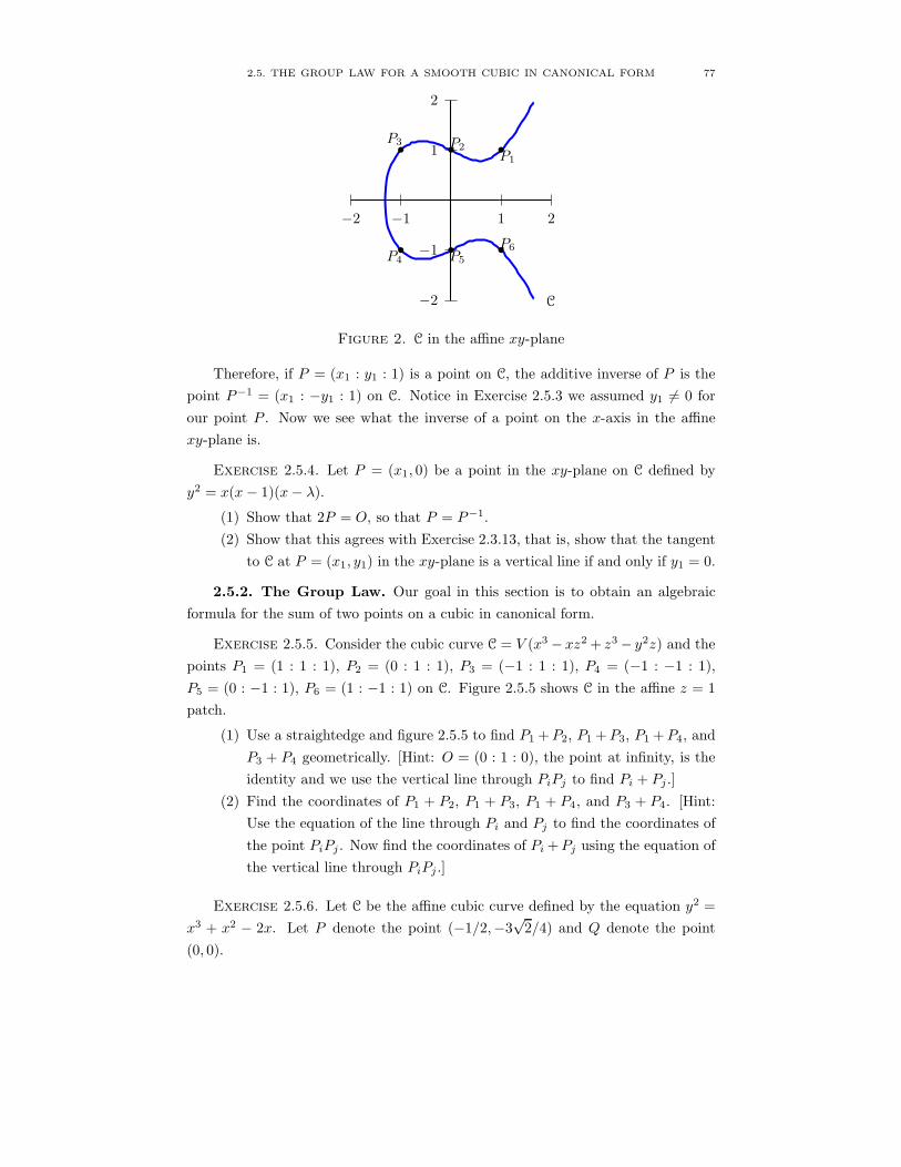
2.5. THE GROUP LAW FOR A SMOOTH CUBIC IN CANONICAL FORM 77
1
2
−1
−2
1 2−1−2
C
•P1•P2•P3
•P4•P5
•P6
Figure 2. C in the affine xy-plane
Therefore, if P = (x1 : y1 : 1) is a point on C, the additive inverse of P is the
point P−1 = (x1 : −y1 : 1) on C. Notice in Exercise 2.5.3 we assumed y1 6= 0 for
our point P . Now we see what the inverse of a point on the x-axis in the affine
xy-plane is.
Exercise 2.5.4. Let P = (x1, 0) be a point in the xy-plane on C defined by
y2 = x(x − 1)(x− λ).
(1) Show that 2P = O, so that P = P−1.
(2) Show that this agrees with Exercise 2.3.13, that is, show that the tangent
to C at P = (x1, y1) in the xy-plane is a vertical line if and only if y1 = 0.
2.5.2. The Group Law. Our goal in this section is to obtain an algebraic
formula for the sum of two points on a cubic in canonical form.
Exercise 2.5.5. Consider the cubic curve C = V (x3 − xz2 + z3 − y2z) and the
points P1 = (1 : 1 : 1), P2 = (0 : 1 : 1), P3 = (−1 : 1 : 1), P4 = (−1 : −1 : 1),
P5 = (0 : −1 : 1), P6 = (1 : −1 : 1) on C. Figure 2.5.5 shows C in the affine z = 1
patch.
(1) Use a straightedge and figure 2.5.5 to find P1 +P2, P1 +P3, P1 +P4, and
P3 + P4 geometrically. [Hint: O = (0 : 1 : 0), the point at infinity, is the
identity and we use the vertical line through PiPj to find Pi + Pj .]
(2) Find the coordinates of P1 + P2, P1 + P3, P1 + P4, and P3 + P4. [Hint:
Use the equation of the line through Pi and Pj to find the coordinates of
the point PiPj . Now find the coordinates of Pi+Pj using the equation of
the vertical line through PiPj .]
Exercise 2.5.6. Let C be the affine cubic curve defined by the equation y2 =
x3 + x2 − 2x. Let P denote the point (−1/2,−3√2/4) and Q denote the point
(0, 0).

78 2. CUBIC CURVES AND ELLIPTIC CURVES
(1) Write the defining equation of C in canonical form and verify that P and
Q are on C.
(2) Find the equation of `(P,Q), the line through P and Q.
(3) Find the coordinates of the point PQ on C, that is, the coordinates of the
third point of intersection of C and `(P,Q).
(4) Let O denote the inflection point (0 : 1 : 0) and find the coordinates of
the point P +Q on C using O as the identity element.
(5) Find the coordinates of 2P on C.
(6) Find the coordinates of the point P−1 on C usingO as the identity element.
(7) Show that 2Q = O. [Hint: Show that the tangent to C at Q passes through
O and invoke Exercise 2.3.13.]
(8) Find the coordinates of all three points of the points of order 2 on C.
Now we carry out these computations in a more general setting to derive an
expression for the coordinates of P +Q. Let C = V (x(x − z)(x − λz) − y2z) be a
smooth cubic curve. Dehomogenize the defining equation x(x−z)(x−λz)−y2z = 0
to get the affine equation y2 = f(x), where f(x) = x(x − 1)(x− λ).
Exercise 2.5.7. Suppose P = (x1 : y1 : 1) and Q = (x2 : y2 : 1) are two points
on C, with Q 6= P−1 (that is x1 6= x2), and let y = αx + β be the equation of line
`(P,Q) through the points P and Q.
(1) Suppose P 6= Q. Express α in terms of x1, x2, y1, y2.
(2) Suppose P = Q (in which case `(P,Q) is the tangent line to C at P ). Use
implicit differentiation to express α in terms of x1, y1.
(3) Substitute αx + β for y in the equation y2 = f(x) to get a new equation
in terms of x only. Write the resulting equation of x in the form x3 +
Bx2 + Cx +D = 0.
(4) If P + Q has coordinates (x3 : y3 : 1), explain why x3 + Bx2 + Cx +D
must factor as (x− x1)(x − x2)(x− x3).
(5) By equating coefficients of x2 in parts (4) and (5), conclude that
x3 = −x1 − x2 + α2 + λ+ 1,
where α is the slope of the line `(P,Q).
(6) We now have an expression for the x-coordinate of P + Q. Use this to
conclude that
P +Q =(−x1 − x2 + α2 + λ+ 1 : y1 + α(x3 − x1) : 1
)
where α is the slope of `(P,Q). [Hint: Use the relationship between the
y-coordinates of PQ and P + Q along with the fact that (x1, y1) lies on
the line defined by y = αx+ β.]

2.5. THE GROUP LAW FOR A SMOOTH CUBIC IN CANONICAL FORM 79
Therefore, if P = (x1 : y1 : 1), P = (x2 : y2 : 1) are points on C = V (x(x −1)(x− λ)− y2), then P +Q has coordinates (x3 : y3 : 1) given by
x3 =
−x1 − x2 + λ+ 1 +
(y2 − y1x2 − x1
)2
if P 6= Q
−2x1 + λ+
(f ′(x1)
2y1
)2
if P = Q
y3 = y1 + α(x3 − x1).
Exercise 2.5.8. Verify the results in Exercise 2.5.6 using the above formula.
We may perform a similar sequence of calculations for a cubic in general form.
Let C be the cubic curve defined by y2z = ax3+bx2z+cxz2+dz3, where a, b, c, d ∈ C.Dehomogenize this defining equation to get the affine equation y2 = f(x), where
f(x) = ax3 + bx2 + cx+ d and f has distinct roots.
Exercise 2.5.9. Suppose P = (x1 : y1 : 1) and Q = (x2 : y2 : 1) be two points
on C, with Q 6= P−1, and let y = αx + β be the equation of line `(P,Q) through
the points P and Q.
(1) Suppose P 6= Q. Express α in terms of x1, x2, y1, y2.
(2) Suppose P = Q (in which case `(P,Q) is the tangent line to C at P ). Use
implicit differentiation to express α in terms of x1, y1.
(3) Substitute αx + β for y in the equation y2 = f(x) to get a new equation
in terms of x only. Write the resulting equation of x in the form x3 +
Bx2 + Cx +D = 0.
(4) If P +Q has coordinates P +Q = (x3 : y3 : 1), explain why Ax3 +Bx2 +
Cx+D must factor as a(x − x1)(x − x2)(x − x3).
(5) By equating coefficients of x2, conclude that
x3 = −x1 − x2 +α2 − b
a,
where α is the slope of the line `(P,Q).
(6) We now have an expression for the x-coordinate of P + Q. Use this to
conclude that
P +Q =
(−x1 − x2 −
b
a+
1
aα2 : y1 + α(x3 − x1) : 1
)
where α is the slope of `(P,Q).
80 2. CUBIC CURVES AND ELLIPTIC CURVES
Therefore, if P = (x1 : y1 : 1), P = (x2 : y2 : 1) are points on C = V (ax3 +
bx2 + cx+ d− y2), then P +Q has coordinates (x3 : y3 : 1) given by
x3 =
−x1 − x2 −b
a+
1
a
(y2 − y1x2 − x1
)2
if P 6= Q
−2x1 −b
a+
1
a
(f ′(x1)
2y1
)2
if P = Q
y3 = y1 + α(x3 − x1).
2.5.3. Rational Points on Cubics. Of particular importance to number
theory and the theory of elliptic curves is the following property of the group law
for elliptic curves.
Definition 2.5.1. Let y2 = f(x) be an affine equation of a smooth cubic
curve, where f(x) is a polynomial with rational coefficients. A point P = (x, y) is
a rational point if x, y ∈ Q.
Once we have a rational point, a natural follow-up would be to ask how many
rational points exist on a given curve. We first note the following property of
rational points.
Exercise 2.5.10. Let y2 = f(x) be an affine equation of a smooth cubic curve,
where f(x) is a degree three polynomial with rational coefficients. Suppose P and
Q are rational points on this curve, so that P,Q ∈ Q2 and Q 6= P−1. Prove that
P +Q is also a rational point.
What happens if Q = P−1? In this case P +Q would be equal to the point at
infinity O = [0 : 1 : 0]. While this point does have rational coordinates, this point
is technically not on this particular affine chart. How can we address this?
2.5.4. Cubics over Other Fields. Another important consequence of our
algebraic formulation for the group law is that the operations involved are inde-
pendent of the field of definition. With this addition law, we can define the group
law for cubic curves not only over C, but also over R, Q, and even over finite fields.
However, there is one subtlety that we need to be aware of. Some of the calculations
need to be modified if the characteristic of the field is equal to 2.
Exercise 2.5.11. This is inspired by [AG06], pages 105–109. Let C be the
cubic curve given by y2 = x3 + 1.
(1) Show that (0, 4) and (2, 3) are points of C over F5.
(2) Use the formulas for addition above to compute (0, 4) + (2, 3).
(3) Find all of the points on C that are defined over F5.

2.6. CUBICS AS TORI 81
2.6. Cubics as Tori
The goal of this problem set is to realize a smooth cubic curve in P2(C) as a torus.
Exercise 2.6.1. Draw a sequence of diagrams to show that if we attach the
circle A to the circle C and the circle B to circle D, we obtain a torus.
A B
C D
Exercise 2.6.2. Let T : [0, 2π] → C be defined by T (θ) = eiθ and let f : C→ C
be defined by f(x) =√x.
(1) Show that T ([0, 2π]) is a unit circle in C.
(2) Show that f T ([0, 2π]) is a half circle.
Exercise 2.6.3. Now let T : [0, 2π] → C be defined by T (θ) = 2eiθ and let
f : C→ C be defined by f(x) =√x(x− 1).
(1) Show that T ([0, 2π]) is a circle of radius 2 in C.
(2) Show that f T (0) = f T (2π).(3) Show that f T ([0, 2π]) is a closed curve in C− [0, 1].
(4) Sketch an intuitive argument for f(x) =√x(x − 1) being well-defined on
C− [0, 1] in two ways: (i) by setting√
2(2− 1) = +√2, and then (ii) by
setting√2(2− 1) = −
√2. This construction establishes a 2 sheeted cover
of C.
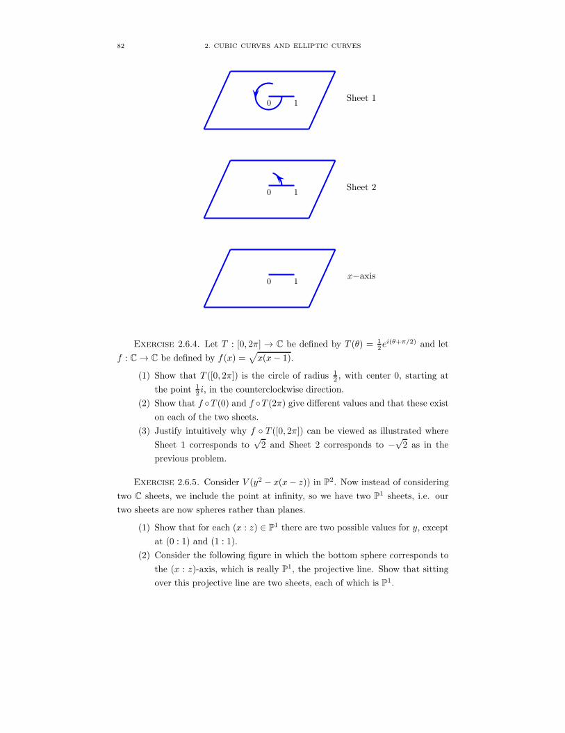
82 2. CUBIC CURVES AND ELLIPTIC CURVES
Sheet 10 1
Sheet 20 1
x−axis0 1
Exercise 2.6.4. Let T : [0, 2π] → C be defined by T (θ) = 12ei(θ+π/2) and let
f : C→ C be defined by f(x) =√x(x− 1).
(1) Show that T ([0, 2π]) is the circle of radius 12 , with center 0, starting at
the point 12 i, in the counterclockwise direction.
(2) Show that f T (0) and f T (2π) give different values and that these exist
on each of the two sheets.
(3) Justify intuitively why f T ([0, 2π]) can be viewed as illustrated where
Sheet 1 corresponds to√2 and Sheet 2 corresponds to −
√2 as in the
previous problem.
Exercise 2.6.5. Consider V (y2 − x(x− z)) in P2. Now instead of considering
two C sheets, we include the point at infinity, so we have two P1 sheets, i.e. our
two sheets are now spheres rather than planes.
(1) Show that for each (x : z) ∈ P1 there are two possible values for y, except
at (0 : 1) and (1 : 1).
(2) Consider the following figure in which the bottom sphere corresponds to
the (x : z)-axis, which is really P1, the projective line. Show that sitting
over this projective line are two sheets, each of which is P1.

2.7. CROSS-RATIOS AND THE J-INVARIANT 83
Sheet 1(0:1) (1:1)
Sheet 2(0:1) (1:1)
x−axis(0:1) (1:1)
(3) Replace the segments in [(0 : 1), (1 : 1)] in Sheets 1 and 2 with circles A
and B. Draw a sequence of diagrams to show that if we attach circle A
in Sheet 1 to circle B in Sheet 2, then we obtain a sphere.
(4) Conclude that V (y2 − x(x − z)) ⊂ P2 is a sphere.
Exercise 2.6.6. Now consider f : C→ C defined by f(x) =√x(x − 1)(x− λ).
(1) Justify that f is well-defined on two possible sheets.
(2) Show that f is a 2-to-1 cover of the x-axis except at x = 0, x = 1, and
x = λ.
(3) Homogenize y2 = x(x− 1)(x− λ) to show that we now have a two-to-one
cover of P1 except at (0 : 1), (1 : 1), (λ : 1), and (1 : 0), where each of the
two sheets is itself a P1. Explain how this is related to (b). What is the
extra ramified point?
(4) Use the earlier exercises to draw a sequence of diagrams illustrating how
y2 = x(x− z)(x− λz) in P2 is a torus.
2.7. Cross-Ratios and the j-Invariant

84 2. CUBIC CURVES AND ELLIPTIC CURVES
We have seen that every smooth cubic curve can be thought of as a two-to-one
cover of P1, branched at exactly four points. This section will show how we can
always assume, via a change of coordinates, that three of these four branch points
are (1 : 0), (1 : 1) and (0 : 1). We will start with a series of exercises that explicitly
give these changes of coordinates. We then will have a series of exercises putting
these changes of coordinates into changes of coordinates of C. It is here that the
cross ratio is made explicit. The key behind all of this is that two ordered sets of
four points are projectively equivalent if and only if they have the same cross-ratio.
The cross ratio will then return us to the j-invariant for a cubic curve.
2.7.1. Projective Changes of Coordinates for P1. Given any three points
(x1 : y1), (x2 : y2), (x3 : y3) ∈ P1, we want to find a projective change of coordinates
T : P1 → P1 such that
T (x1 : y1) = (1 : 0)
T (x2 : y2) = (0 : 1)
T (x3 : y3) = (1 : 1)
We will see that not only does such a map always exist, but that it is unique.
We first have to define what we mean by a projective change of coordinates for
P1. In Section 1.5, we gave a definition for project change of coordinates for P2.
The definition for P1 is similar, namely that a projective change of coordinates is
given by
u = ax+ by
v = cx+ dy,
where ad− bc 6= 0. We write this as
T (x : y) = (ax + by : cx+ dy).
Now, we could write (x : y) ∈ P1 as a column vector(x
y
).
If we let
A =
(a b
c d
),
then we can think of T (x : y) = (ax + by : cx + dy) in terms of the matrix
multiplication
A
(x
y
)=
(a b
c d
)(x
y
)=
(ax+ by
cx+ dy
).
2.7. CROSS-RATIOS AND THE J-INVARIANT 85
In P1, we have that (x : y) = (λx : λy) for any constant λ 6= 0. This suggests the
following:
Exercise 2.7.1. Show that the matrices
A =
(3 2
1 4
)and B =
(6 4
2 8
)= 2 · A
give rise to the same change of coordinates of P1 → P1.
Exercise 2.7.2. Show that the matrices
A =
(a b
c d
)and B =
(λa λb
λc λd
),
for any λ 6= 0, give rise to the same change of coordinates of P1 → P1.
This means that the projective change of coordinates
(x : y) → (ax+ by : cx+ dy)
and
(x : y) → (λax + λby : λcx+ λdy)
are the same.
Our desired projective change of coordinates T such that
T (x1 : y1) = (1 : 0), T (x2 : y2) = (0 : 1), T (x3 : y3) = (1 : 1)
is
T (x : y) = ((x2y − y2x)(x1y3 − x3y1) : (x1y − y1x)(x2y3 − x3y2)).
(It should not be at all clear how this T was created.)
Exercise 2.7.3. Let
(x1 : y1) = (1 : 2), (x2 : y2) = (3 : 4), (x3 : y3) = (6 : 5).
Show that
(1) T (x : y) = (28x− 21y : 18x− 9y)
(2) T (1 : 2) = (1 : 0), T (3 : 4) = (0 : 1), T (6 : 5) = (1 : 1)
These problems give no hint as to how anyone could have known how to create
T ; the goal of these last problems was to show that this T actually does work.
We now want to start looking at uniqueness questions.
86 2. CUBIC CURVES AND ELLIPTIC CURVES
Exercise 2.7.4. Let T (x : y) = (ax + by : cx + dy) be a projective change of
coordinates such that T (1 : 0) = (1 : 0), T (0 : 1) = (0 : 1), T (1 : 1) = (1 : 1). Show
that
a = d 6= 0
and that
b = c = 0.
Explain why T must be the same as the projective change of coordinates given by
T (x : y) = (x : y).
Part of showing uniqueness will be in finding a decent, easy to use formula for
the inverse of our map T .
Exercise 2.7.5. Let T (x : y) = (ax + by : cx + dy) be a projective change of
coordinates and let
A =
(a b
c d
)
be its associated matrix. Let
B =
(d −b−c a
)
Show that
A ·B = det(A)I,
where I is the two-by-two identity matrix.
Exercise 2.7.6. Let (x1 : y1), (x2 : y2), (x3 : y3) ∈ P1 be three distinct points.Let T1 and T2 be two projective change of coordinates such that
T1(x1 : y1) = (1 : 0), T1(x2 : y2) = (0 : 1), T1(x3 : y3) = (1 : 1)
and
T2(x1 : y1) = (1 : 0), T2(x2 : y2) = (0 : 1), T2(x3 : y3) = (1 : 1).
Show that T1 T−12 is a projective change of coordinates such that
T1 T−12 (1 : 0) = (1 : 0), T1 T−1
2 (0 : 1) = (0 : 1), T1 T−12 (1 : 1) = (1 : 1).
Show that T1 and T2 must be the same projective change of coordinates.
Thus our desired map T is unique.
Exercise 2.7.7. Mathematicians will say that any three points in P1 can be
sent to any other three points, but any fourth point’s image must be fixed. Using
the results of this section, explain what this means. (This problem is not so much
a typical math exercise but is instead an exercise in exposition.)

2.7. CROSS-RATIOS AND THE J-INVARIANT 87
Finally, we can see how anyone ever came up with the map
T (x : y) = ((x2y − y2x)(x1y3 − x3y1) : (x1y − y1x)(x2y3 − x3y2)).
We just have to find a matrix
A =
(a b
c d
)
such that
A
(x1
y1
)=
(1
0
), A
(x2
y2
)=
(0
1
), A
(x3
y3
)=
(1
1
).
Solving for the coefficients for A is now just a (somewhat brutal) exercise in algebra.
2.7.2. Working in C. Algebraic geometers like to work in projective space
Pn. Other mathematicians prefer to keep their work in affine spaces, such as Cn,
allowing for points to go off, in some sense, to infinity. In this subsection we
interpret the projective change of coordinates T : P1 → P1 in the previous section
as a map T : C ∪ ∞ → C ∪ ∞.Given three points x1, x2 and x3 in C, we want to find a map T : C ∪ ∞ →
C ∪ ∞ such that
T (x1) = ∞T (x2) = 0
T (x3) = 1
For now, set
T (x) =(x2 − x)(x1 − x3)
(x1 − x)(x2 − x3).
The next three exercises are in parallel with those in the previous subsection.
Exercise 2.7.8. Let x1 = 1/2, x2 = 3/4, and x3 = 6/5. (Note that these
correspond to the dehomogenization of the three points (x1 : y1) = (1 : 2), (x2 :
y2) = (3 : 4) in the previous subsections first problem.) Show that
(1) T (x) =28x− 21
18x− 9.
(2) T (1/2) = ∞, T (3/4) = 0, T (6/5) = 1.
The next exercise will link the map T : C ∪ ∞ → C ∪ ∞ with the map
T : P1 → P1. Recall in P1 that
(x : y) = (x
y: 1),
provided that y 6= 0. By a slight abuse of notation, we can think of dehomogenizing
as just setting all of the y’s equal to one.

88 2. CUBIC CURVES AND ELLIPTIC CURVES
Exercise 2.7.9. Show that the map T : P1 → P1 given by
T (x : y) = (ax+ by : cx+ dy)
will correspond to a map T : C ∪ ∞ → C ∪ ∞ given by
T (x) =ax+ b
cx+ d.
Exercise 2.7.10. Show that the map T : P1 → P1 given by
T (x : y) = ((x2y − y2x)(x1y3 − x3y1) : (x1y − y1x)(x2y3 − x3y2))
will correspond to the map T : C ∪ ∞ → C ∪ ∞ given by
T (x) =(x2 − x)(x1 − x3)
(x1 − x)(x2 − x3).
Here the dehomogenization is the map achieved by setting y = 1.
2.8. Cross Ratio: A Projective Invariant
Suppose we are given some points in P1. We can label these points in many
ways, by choosing different coordinate systems. This is the same as studying the
points under projective changes of coordinates. We would like to associate to our
points something (for us, a number) that will not change, no matter how we write
the points. We call such numbers invariants.
If we start with three points p1 = (x1 : y1), p2 = (x2 : y2), p3 = (x3 : y3) ∈ P1,no such invariant number can exist, since any three points can be sent to any other
three points. But we cannot send any four points to any other four points. This
means that any collection of four points has some sort of intrinsic geometry. So
add a fourth point p4 = (x4 : y4) ∈ P1. Then
Definition 2.8.1. The cross ratio of the four distinct points p1, p2, p3, p4 is
[p1, p2, p3, p4] =(x2y4 − y2x4)(x1y3 − x3y1)
(x1y4 − y1x4)(x2y3 − x3y2).
We need to show that this number does not change under projective change of
coordinates.
Exercise 2.8.1. Let
p1 = (1 : 2), p2 = (3 : 1), p3 = (1 : 1), p4 = (5 : 6).
(1) Calculate the cross ratio [p1, p2, p3, p4].
(2) Let T : P1 → P1 be
T (x : y) = (3x+ 2y : 2x+ y).
Find T (p1), T (p2), T (p3), T (p4).

2.8. CROSS RATIO: A PROJECTIVE INVARIANT 89
(3) Show
[T (p1), T (p2), T (p3), T (p4)] = [p1, p2, p3, p4].
Exercise 2.8.2. Let p1 = (x1 : y1), p2 = (x2 : y2), p3 = (x3 : y3), p4 = (x4 : y4)
be any collection of four distinct points in P1 and let T (x, y) = (ax+ by : cx+ dy)
be any projective change of coordinates. Show
[T (p1), T (p2), T (p3), T (p4)] = [p1, p2, p3, p4].
(This is a long exercise in algebra, but at the end, there should be satisfaction at
seeing everything being equal.)
The above cross ratio depends, though, on how we ordered our four points
p1, p2, p3p4. If we change the order, the cross ratio might change.
Exercise 2.8.3. Let p1, p2, p3, p4 be any four distinct points in P1. Show
[p1, p2, p3, p4] =1
[p2, p1, p3, p4].
Exercise 2.8.4. Let p1 = (x1 : y1), p2 = (x2 : y2), p3 = (x3 : y3), p4 = (x4 : y4)
such that [p1, p2, p3, p4] 6= ±1. Show that there is no projective change of coordinate
T (x : y) = (ax+ by : cx+ dy) such that T interchanges p1 with p2 but leave p3 and
p4 alone. In other words, show there is no T such that
T (p1) = p2, T (p2) = p1, T (p3) = p3, T (p4) = p4.
Exercise 2.8.5. Let p1 = (x1 : y1), p2 = (x2 : y2), p3 = (x3 : y3), p4 = (x4 : y4)
be any collection of four distinct points in P1. Show that
[p2, p1, p4, p3] = [p1, p2, p3, p4].
Exercise 2.8.6. Using the notation from the previous problem, find two other
permutations of the points p1, p2, p3, p4 so that the cross ratio does not change.
Let
[p1, p2, p3, p4] = λ.
We have shown that there are four permutations of the p1, p2, p3, p4 that do not
change the cross ratio but we have also shown
[p2, p1, p3, p4] =1
λ.
Exercise 2.8.7. Using the above notation, find permutations of the p1, p2, p3, p4
so that all of the following cross ratios occur:
λ,1
λ,
1
1− λ, 1− λ,
λ
λ− 1,λ− 1
λ.

90 2. CUBIC CURVES AND ELLIPTIC CURVES
Exercise 2.8.8. Given any four distinct points p1, p2, p3, p4 in P1, show that
the j-invariant of the cross ratio does not change under any reordering of the four
points and under any projective linear change of coordinates. (This is why we are
justified in using the term “invariant” in the name j-invariant.)
Thus given a smooth cubic curve, we can put the curve into Weierstrass normal
form and associate to this curve a singe number j. A natural question is if two
different curves could have the same j invariant. The next exercises will show that
this is not possible.
Exercise 2.8.9. Suppose that
j(λ) = 28(λ2 − λ+ 1)3
λ2(λ− 1)2= a
for some constant a.
(1) Show that any solution µ of the equation
28(λ2 − λ+ 1)3 − aλ2(λ − 1)2 = 0
has the property that
j(µ) = a.
(2) Show that the above equation can have only six solutions.
(3) Show that if λ is a solution, then the other five solutions are 1λ ,
11−λ , 1−
λ, λλ−1 ,
λ−1λ .
(4) Show that if we have two curves zy2 = x(x − z)(x − λz) and zy2 =
x(x − z)(x− µz) with
j(λ) = j(µ),
then there is a projective change of coordinates of P1 with coordinates
(x : z) taking the first curve to the second.
2.9. Torus as C/Λ
We will begin this section with background material from abstract algebra to
make clear what a quotient group is. After that material is developed, we will
expeditiously proceed to the goal of this problem set, namely to realize a torus as
the quotient group C/Λ.

2.9. TORUS AS C/Λ 91
2.9.1. Quotient Groups. Given a group G with binary operation ?, a subset
S of G is said to be a subgroup if, equipped with the restriction of ? to S × S, S
itself is a group. Given a known group G, a way to generate examples of groups is
to look at all its subgroups. Another way of generating examples is to “collapse”
a certain type of subgroup N of the group G into the identity element of a new
“quotient group” G/N . In order for this “quotient” construction to yield a group,
N must satisfy certain properties that make it a so-called normal subgroup of G.
Notation: Let G be a group with binary operation ?. This binary operation ?
induces an operation ? (by abuse of notation) on subsets of G defined as follows:
if S and T are subsets of G, then S ? T := s ? t : s ∈ S, t ∈ T . If S = s is a
singleton, then we write sT for s ? T ; likewise, we write St for S ? t.
Definition 2.9.1. Given a nonempty set A, we say that a collection P of
subsets of A is a partition of A if P consists of nonempty, pairwise disjoint sets
whose union is A. This means that if
P = Uαα∈I ,
where I is an indexing set, then the elements of P satisfy the following two condi-
tions.
(1) Pα ∩ Pβ = for all α, β ∈ I;
(2) A = ∪α∈IUα.
Exercise 2.9.1. Let A be a nonempty set.
(1) Let ∼ be an equivalence relation on the set A. Show that the set of
equivalence classes of ∼ is a partition of A.
(2) Suppose P is a partition of A. Show that the relation ∼, defined by x ∼ y
if and only if x and y belong to the same element of P , is an equivalence
relation.
The previous exercise shows that partitions give natural equivalence relations
and that equivalence relations are natural ways of generating partitions.
Definition 2.9.2. Let G be a group. A quotient group of G is a partition of
G that is a group under the subset operation induced by the binary operation on
G.
Exercise 2.9.2. For i = 0, 1, 2, let 3Z + i := 3n + i : n ∈ Z. Show that
3Z, 3Z+ 1, 3Z+ 2 is a quotient group of the additive group Z.
Exercise 2.9.3. Suppose Q is a quotient group of a group G. Prove the
following.
92 2. CUBIC CURVES AND ELLIPTIC CURVES
(1) Let e be the identity of G and let E be the unique element of Q with
e ∈ E. Then E is the identity in the group Q.
(2) Let A ∈ Q, a ∈ A, and a−1 the inverse to a in G. Let A′ be the unique
element of Q containing a−1. Then A′ is the inverse to A in Q.
(3) Let A ∈ Q. For any a ∈ A, A = aE = Ea.
Definition 2.9.3. Let G be a group. A normal subgroup N of G is a subgroup
of G that is the identity element of some quotient group Q of G. The subsets of G
in Q are called the cosets of N . If N is a normal subgroup by virtue of being the
identity element of the quotient group Q, we write Q = G/N and say that Q is the
group G mod N .
Exercise 2.9.4. Identify all possible normal subgroups of the additive group
Z. (Hint: start by analyzing the previous exercise.)
Recall, from above, that gN = gn : n ∈ N. In the next exercise we will
establish that N is normal if and only if gN = Ng. gN and Ng are two sets and
we will show equality as sets. In particular, we show that every element of gN is
in Ng and vice versa, but it is not necessarily true that gn = ng for a particular
n ∈ N , i.e. the group need not be abelian.
Exercise 2.9.5. Show that a subgroup N of a group G is normal if and only if
gN = Ng for all g ∈ G. [Hint: If gN = Ng for all g ∈ G, define Q = gN : g ∈ G.Show that the operation on subsets of G is well-defined on Q and makes Q into a
group.]
Exercise 2.9.6. Given a quotient group Q of a group G, show that the element
of Q containing e (the identity element of G) is a normal subgroup of G.
Exercise 2.9.7. Suppose G is an abelian group. Show that every subgroup is
normal.
In the discussion above, we have produced some ways of generating examples of
groups: finding subgroups and taking quotients. (To be sure, there are more ways
of generating groups from given ones: for instance, one can take direct products, or
ultraproducts, but that’s not useful to us at this point.) But how do we compare
groups? One way of doing this is to look for maps between groups that preserve
group structure.
Definition 2.9.4. Suppose (G, ?G) and (H, ?H) are two groups. A map ϕ :
G→ H is said to be a homomorphism if ϕ(x ?G y) = ϕ(x) ?H ϕ(y) for all x, y ∈ G.
If a homomorphism is bijective, we call it an isomorphism and say that the groups
G and H are isomorphic. We denote this by G ∼= H .
2.9. TORUS AS C/Λ 93
If two groups are isomorphic, they are essentially “the same.” If there is a
homomorphism between two groups there is still a nice relationship between G and
H .
Exercise 2.9.8. Let ϕ : G→ H be a homomorphism, and let e be the identity
element of H . Let ker(ϕ) := g ∈ G : ϕ(g) = e. (We call ker(ϕ) the kernel of ϕ.)
(1) Show that ker(ϕ) is a subgroup of G.
(2) Show that ker(ϕ) is a normal subgroup of G.
(3) Show that if ϕ : G → H is onto, then the quotient group G/ker(ϕ) is
isomorphic to H .
The previous exercise gives us a way to check whether a subset S of a groupG is
a normal subgroup. If we can realize the subset S as the kernel of a homomorphism,
then it must be a normal subgroup.
Exercise 2.9.9. LetG be the multiplicative group of all invertible 2×2 matrices
over the real numbers, and let N be the subset of G consisting of matrices having
determinant equal to 1. Prove that N is a normal subgroup of G.
2.9.2. The Torus. In order to understand some of the geometry of a torus,
we need to determine how a torus is formed. We will begin by using a little group
theory to realize a circle, S1, as the quotient group R/Z.
Exercise 2.9.10.
(1) Show that R is an abelian group under addition.
(2) Show that Z is a subgroup of R and conclude that Z is a normal subgroup.
Exercise 2.9.11. Define a relation on R by x ∼ y if and only if x− y ∈ Z.(1) Verify that ∼ an equivalence relation.
(2) Let [x] denote the equivalence class of x, that is, [x] = y ∈ R | x ∼ y.Find the following equivalence classes: [0], [ 12 ], and [
√2].
(3) The equivalence relation ∼ gives a partition of R. Explain how this par-
tition R/Z is the realization of a circle. [Hint: Explain how progressing
from 0 to 1 is the same as going around a circle once.]
We can also use Exercise 2.9.8 to give an isomorphism between R/Z and the
circle. Let S1 denote the unit circle centered at the origin in R2. As we have already
seen R2 is in one-to-one correspondence with C, so we can regard S1 as the set
S1 = x ∈ C | |x| = 1. Recall, that any complex number has a polar representation
x = r(cos θ + i sin θ), so we can express S1 as S1 = cos θ + i sin θ : θ ∈ R ⊂ C.
Exercise 2.9.12. Show that S1 is a group under (complex) multiplication.
94 2. CUBIC CURVES AND ELLIPTIC CURVES
Exercise 2.9.13. Define a map φ : R→ S1 by φ(θ) = cos 2πθ + i sin 2πθ.
(1) Show that φ is onto.
(2) Show that φ is a homomorphism, i.e. show that φ(α+ β) = φ(α)φ(β) for
all α, β ∈ R.(3) Find kerφ and conclude that R/Z ∼= S1.
We now want to extend the ideas in the previous exercises to the complex plane.
Let ω1 and ω2 be complex numbers such that ω1
ω2is not purely real. Let the integer
lattice Λ be defined as Λ = mω1+nω2 : m,n ∈ Z. We will call the parallelogram
formed by joining 0, ω1, ω1 + ω2, ω2, and 0 in succession the fundamental period-
parallelogram. We will realize a torus as a quotient group C/Λ.
Exercise 2.9.14. (1) Sketch the lattice generated by ω1 = 1 and ω2 = i.
[Hint: Sketch the fundamental period-parallelogram of this lattice.]
(2) Sketch the lattice generated by ω1 = 1 + i and ω2 = i.
Exercise 2.9.15. (1) Show that C is an abelian group under addition.
(2) Show that Λ is a subgroup of C and conclude that Λ is a normal subgroup.
Exercise 2.9.16. Define a relation on C by x ∼ y if and only if x − y ∈ Λ.
Show that ∼ is an equivalence relation.
Since ∼ is an equivalence relation, it is natural to ask about the quotient group
C/Λ.
Exercise 2.9.17. Let Λ ⊂ C be the integer lattice generated by ω1 = 1, ω2 =
i and let a, b ∈ R.(1) Find all points in C equivalent to 1
2 + 12 i in the group C/Λ.
(2) Find all points in C equivalent to 13 + 1
4 i in C/Λ.
(3) Show that a ∼ a+ i in C/Λ.
(4) Show that bi ∼ 1 + bi in C/Λ.
Exercise 2.9.18. Sketch a sequence of diagrams to show that C/Λ is a torus.
[Hint: Construct a torus using ω1 = 1 and ω2 = i by identifying the horizontal and
vertical sides of the fundamental period-parallelogram as in the previous problem.
Now repeat with any lattice.]
Exercise 2.9.19. Let Λ ⊂ C be the integer lattice generated by ω1 = 1, ω2 =
i.(1) Sketch a vertical segment in the fundamental period-parallelogram and
illustrate to what this corresponds on our torus. Sketch a horizontal line
in the fundamental period-parallelogram and illustrate to what this cor-
responds on our torus.

2.10. MAPPING C/Λ TO A CUBIC 95
(2) Show that 14 + i ∈ C/Λ has order 4 and write all of the elements of 〈14 + i〉.
(3) Represent the fact that 14 + i has order 4 geometrically on the fundamen-
tal period-parallelogram by sketching a line in C that has slope 14 and
considering its image in C/Λ.
(4) Sketch the paths traced by these segments on the torus. What do you
notice about this path on the torus?
(5) Pick any element α ∈ C/Λ and show that if α has finite order, then the
path on the torus represented by the line through 0 and α is a closed path.
(6) Suppose an element α has infinite order. What can you say about the
slope of the line through 0 and α. Illustrate this phenomenon on the
fundamental period-parallelogram in C and on the torus.
2.10. Mapping C/Λ to a Cubic
The goal of this problem set is construct a map from C/Λ to a cubic curve.
In this section we assume some knowledge about complex variables and analysis.
For a quick outline of the basics that we are going to use, please refer to Appendix A
or your favorite introductory complex variables textbook.
We have established that given any smooth cubic curve C we can realize C
topologically as a torus. We have also seen that given any integer lattice Λ =
mω1 + nω2 : m,n ∈ Z ⊂ C, with ω1/ω2 not purely real, we can construct a torus
C/Λ. Our goal in this section is to generate a smooth cubic curve given a lattice Λ.
Hence, we will construct a map from the quotient group C/Λ to C2 whose image is
the zero locus of a non-singular cubic polynomial. In order to do this we will use
the Weierstrass ℘-function ℘ : C/Λ → C defined by
℘(x) =1
x2+
∑
m,n∈Z
(m,n) 6=(0,0)
1
(x −mω1 − nω2)2− 1
(mω1 + nω2)2.
Then our map C/Λ → C2 will be given by the map x 7→ (℘(x), ℘′(x)), and the
smooth cubic will be defined by the differential equation [℘′(x)]2 = 4[℘(x)]3 +
A℘(x) +B.
At this point it is not at all clear how we arrived at the function ℘. We begin
by considering the minimal properties that are essential for our map C/Λ → C. We
will then show that ℘ has these properties and gives us our desired cubic.
Exercise 2.10.1. Show that for a function f : C/Λ → C to be well-defined,
the function f : C→ C must be doubly-periodic, that is,
f(x+ ω1) = f(x) and f(x+ ω2) = f(x),
for all x in the domain of f .

96 2. CUBIC CURVES AND ELLIPTIC CURVES
To define the function f we seek we need only consider what happens on the
fundamental period-parallelogram. Our first hope is that f is analytic on its fun-
damental period-parallelogram, i.e. f has a Taylor series, f(x) =∑∞
n=0 anxn. This
will not work.
Exercise 2.10.2. Show that if a doubly-periodic function f is analytic on
its fundamental period-parallelogram, then f is constant. (Hint: Use Liouville’s
Theorem.)
We see then that f cannot be analytic on its entire fundamental period-parallelogram.
The next hope is that f is be analytic except with a single pole at 0, and hence at
the other lattice points by double periodicity. Furthermore, we hope that the pole
at 0 is not too bad. We can do this, but 0 will be a pole of order two, as the next
two exercises illustrate.
It is inconvenient to integrate over these parallelograms if the singularities are
on the boundaries, but we can translate the vertices, without rotating, so that the
singularities are in the interior. The translated parallelograms will be called cells.
Exercise 2.10.3. Show that the sum of the residues of f at its poles in any
cell is zero.
Exercise 2.10.4. Show that if f has a single pole at 0 in its fundamental
period-parallelogram, not including the other vertices, then 0 must be a pole of
order at least two.
We have now established that a candidate for our function could have the form
f(x) =a−2
x2+ a0 + a1x+ a2x
2 + . . .
Exercise 2.10.5. Show that if
f(x) =a−2
x2+ a0 + a1x+ a2x
2 + a3x3 + . . .
is doubly-periodic, then f is an even function, i.e. a1 = a3 = · · · = 0. [Hint:
Consider the function f(x)− f(−x).]
We can change coordinates to eliminate a0 so that f is now of the form
f(x) =a−2
x2+ a2x
2 + a4x4 + . . .
Now we are ready to introduce the Weierstrass ℘-function.
(2.11) ℘(x) =1
x2+
∑
m,n∈Z
(m,n) 6=(0,0)
1
(x −mω1 − nω2)2− 1
(mω1 + nω2)2,
A series∑∞n=0 an is absolutely convergent whenever
∑∞n=0 |an| <∞.

2.10. MAPPING C/Λ TO A CUBIC 97
A series of functions fn is uniformly convergent with limit f if for all ε > 0,
there exists a natural number N such that for all x in the domain and all n ≥ N ,
|fn(x)− f(x)| < ε.
Exercise 2.10.6. Show that ℘(x) converges uniformly and absolutely except
near its poles. Conclude that ℘(x) is analytic on the complex plane except at the
lattice points Λ = mω1 + nω2.
Since ℘(x) converges uniformly and absolutely, we can differentiate term-by-
term to find ℘′(x), and the order of summation does not affect the value of the
function, so we can rearrange the terms.
Exercise 2.10.7. Find ℘′(x) and show that ℘′(x) is doubly-periodic.
Exercise 2.10.8. Show that ℘(x) is doubly-periodic. (Hint: Consider the
functions Fi(x) = ℘(x+ ωi)− ℘(x) for i = 1, 2.)
Consider the function F (x) = ℘(x) − x−2.
Exercise 2.10.9. Show that F is analytic in a neighborhood of 0.
Exercise 2.10.10. Find the Taylor series expansion of F at 0.
Exercise 2.10.11. From above we know that ℘(x) is even, so F is also even.
Show that the odd powers of x vanish in the Taylor expansion of F at 0.
Exercise 2.10.12. Now we can rewrite ℘(x) = x−2+F (x). Find the coefficients
of x2 and x4 in this expression for ℘(x).
Exercise 2.10.13. Let
g2 = 60∑
ω∈Λ
ω 6=0
1
ω4
and
g3 = 140∑
ω∈Λ
ω 6=0
1
ω6.
Find the x2 and x4 coefficients of ℘(x) in terms of g2 and g3.
Exercise 2.10.14. Find the coefficients of x and x3 in ℘′(x) in terms of g2 and
g3.
We will now establish a cubic relationship between ℘(x) and ℘′(x). In the
previous exercises we found the following expressions for ℘(x) and ℘′(x).
℘(x) =1
x2+
1
20g2x
2 +1
28g3x
4 +O(x6)
℘′(x) = − 2
x3+
1
10g2x+
1
7g3x
3 +O(x5)

98 2. CUBIC CURVES AND ELLIPTIC CURVES
Exercise 2.10.15. Compute ℘(x)3 and ℘′(x)2, and only consider terms up to
first order, that is, find f and g such that ℘(x)3 = f(x) + O(x2) and ℘′(x)2 =
g(x) +O(x2).
Exercise 2.10.16. Show that ℘′(x)2 = 4℘(x)3 − g2℘(x)− g3.

CHAPTER 3
Higher Degree Curves
The goal of this chapter is to explore higher degree curves in P2. There are six
parts. In the first, we define what is meant by an irreducible curve and its degree.
We next show how curves in P2 can be thought of as real surfaces, similar to our
observations for conics (Section 1.7) and cubics (Section 2.6). In the third part, we
develop Bezout’s Theorem, which tells us the number of points of intersection of
two curves. We then introduce the ring of regular functions and the function field
of a curve. In the fourth part, we develop Riemann-Roch, an amazing theorem that
links functions on the curve, the degree of the curve and the genus (the number of
holes) of the curve into one formula. In the last section, we consider singular points
on a curve and develop methods for resolving them.
3.1. Higher Degree Polynomials and Curves
The goals of this section are to define what it means for a curve to be irreducible
and to define the degree of a curve.
In Chapter 1 we dealt with conics, which are the zero sets of second degree
polynomials. In Chapter 2, we looked at cubics, which are the zero sets of third
degree polynomials. It is certainly natural to consider zero sets of higher degree
polynomials.
By now, we know that it is most natural to work in the complex projective
plane, P2, which means in turn that we want our zero sets to be the zero sets of
homogeneous polynomials. Suppose that P (x, y, z) ∈ C[x, y, z] is a homogeneous
polynomial. We denote this polynomial’s zero set by
V(P ) = (a : b : c) ∈ P2 : P (a, b, c) = 0.
Exercise 3.1.1. Let P (x, y, z) = (x+ y+ z)(x2 + y2 − z2). Show that V(P ) is
the union of the two curves V(x+ y + z) and V(x2 + y2 − z2).
Thus, if we want to understand V(P ), we should start with looking at its two
components: V(x + y + z) and V(x2 + y2 − z2). In many ways, this reminds us
99

100 3. HIGHER DEGREE CURVES
of working with prime factorization of numbers. If we understand these build-
ing blocks—those numbers that cannot be broken into a product of two smaller
numbers—then we start to understand the numbers formed when they are strung
together.
Exercise 3.1.2. Let P (x, y, z) = (x+y+z)2. Show that V(P ) = V(x+y+z).
Both (x + y + z)(x2 + y2 − z2) and (x + y + z)2 are reducible, meaning that
both can be factored. We would prefer, for now, to restrict our attention to curves
that are the zero sets of irreducible homogeneous polynomials.
Definition 3.1.1. If the defining polynomial P cannot be factored, we say the
curve V(P ) is irreducible.
When we are considering a factorization, we do not consider trivial factoriza-
tions, such as P = 1 ·P . For the rest of this chapter, all polynomials used to define
curves will be irreducible unless otherwise indicated.
Definition 3.1.2. The degree of the curve V(P ) is the degree of its defining
polynomial, P 1.
The degree of a curve is the most basic number associated to a curve that is
invariant under change of coordinates. The following is an example of this phenom-
enon.
Exercise 3.1.3. Let P (x, y, z) = x3 + y3 − z3. Then V(P ) is a degree three
curve. Consider the projective change of coordinates
x = u− w
y = iv
z = u+ v
Find the polynomial P (u, v, w) whose zero set V(P ) maps to V(P ). Show that
V(P ) also has degree three.
3.2. Higher Degree Curves as Surfaces
The goal of this section is to generalize our work in Sections 1.7 and 2.6, where we
realized smooth conics and cubics over C as topological surfaces over R.
1Recall that we are assuming that all polynomials used to define curves are irreducible. There
will be times when we will define the degree as the degree of P even if P is not irreducible but
then we have to alter slightly the definition of V(P).

3.2. HIGHER DEGREE CURVES AS SURFACES 101
3.2.1. Topology of a Curve. Suppose f(x, y, z) is a homogeneous polyno-
mial, so V(f) is a curve in P2. Recall that the degree of V(f) is, by definition, the
degree of the homogeneous polynomial f . We will see that this algebraic invariant
of the curve is closely linked to the topology of the curve viewed as a surface over
R. Specifically, it is related to the “genus” of the curve, which counts the number
of holes in the surface.
Before we proceed to higher degree curves, we return to our previous experience
with conics and cubics.
Exercise 3.2.1. Consider the conics defined by the homogeneous equation
x2 − y2 = λz2, where λ is a parameter. Sketch affine patches of these in the chart
z = 1 for λ = 4, 1, 0.25.
As λ→ 0, we get x2 − y2 = 0, or (x− y)(x+ y) = 0. In R2, this looks like
•
but this picture isn’t accurate over C in P2. Instead, topologically the picture looks
like “kissing spheres”:
•
Thus, the topological version of the original equation, x2 − y2 = λz2, should be
found by perturbing the kissing spheres a little to account for λ 6= 0:
•
λ = 0 λ 6= 0
∼=
Therefore, by mildly perturbing the specialized, non-smooth conic, we find that
topologically a smooth conic (those in this exercise for which λ 6= 0) is a sphere
with no holes, which agrees with our work in Section 1.7.

102 3. HIGHER DEGREE CURVES
Following this same reasoning, we find another proof that a smooth cubic must
be a torus when realized as a surface over R. We begin with the highly degenerate
cubic, f(x, y, z) = (a1x+ b1y + c1z)(a2x+ b2y + c2z)(a3x+ b3y + c3z). In the real
affine chart z = 1, the picture looks like
•
••
Again, our picture isn’t valid over C in P2. Instead, the correct topological picture
is that of three spheres meeting at three points, as shown.
•
••
Perturbing the top two spheres slightly, we find they join into the topological equiv-
alent of a single sphere, but that this new figure is joined to the third sphere at two
points of contact. Perturbing each of these points of intersection independently of
one another, we obtain a single surface with a hole through the middle as depicted
in the sequence of figures below.
••
∼=
Thus a smooth cubic over C is topologically equivalent to a torus (a sphere with
a hole through it) as a surface over R. Note that this agrees with our results in
Section 2.6.

3.2. HIGHER DEGREE CURVES AS SURFACES 103
Exercise 3.2.2. Mimic the arguments illustrated above to describe the real
surface corresponding to a smooth quartic (fourth degree) curve over C in P2.
Start with a highly degenerate quartic (the product of four pairwise non-parallel
lines), draw the corresponding four spheres, and deform this surface by merging
touching spheres two at a time. How many holes will the resulting figure possess?
Now do the same for a smooth quintic (fifth degree) curve. How many holes
must it have?
3.2.2. Genus of a Curve. The number of holes in the real surfaces corre-
sponding to smooth conics, cubics, quartics and quintics is a topological invariant
of these curves. That is, every smooth conic is topologically equivalent to a real
sphere with no holes. Every smooth cubic is topologically equivalent to a real
torus (a sphere with exactly one hole through it), every smooth quartic is equiv-
alent to a sphere with three holes and every smooth quintic to a sphere with six
holes. Therefore, all smooth conics are topologically equivalent to one another, all
smooth cubics are topologically equivalent, and so on, and each equivalence class
is completely determined by the number of holes in the associated real surface.
Definition 3.2.1. Let V(P ) be a smooth, irreducible curve in P2(C). The
number of holes in the corresponding real surface is called the topological genus of
the curve V(P ).
topological
genus=0topological genus=1 topological genus=2
Presently, this notion of genus only makes sense when we are working over the
reals or an extension of them. However, by the discussion above, we see that there
is a connection between the genus, g, and the degree, d, of a curve. That is, all
smooth curves of degree d have the same genus, so we now wish to find a formula
expressing the genus as a function of the degree.
Exercise 3.2.3. Find a quadratic function in d, the degree of a smooth curve,
that agrees with the topological genus of curves of degrees d = 2, 3, 4 found earlier.
Now use this formula to compute the genus of a smooth quintic (fifth degree) curve.
Does it match your answer to the last exercise?

104 3. HIGHER DEGREE CURVES
Definition 3.2.2. Let V(P ) be a smooth curve of degree d. The number(d− 1)(d− 2)
2is the arithmetic genus of the curve, which is an algebraic invariant
of V(P ).
Exercise 3.2.4. Argue by induction on d, the degree, that the topological
genus agrees with the arithmetic genus for smooth curves, or in other words that
g =(d− 1)(d− 2)
2.
It is a theorem that the topological genus and the arithmetic genus do agree with
one another whenever both are defined and make sense. However, the arithmetic
version is independent of base field and enables us to exploit the genus of curves
even over finite fields in positive characteristic.
3.3. Bezout’s Theorem
The goal of this section is to develop the needed sharp definitions to allow a
statement and a proof of Bezout’s Theorem, which states that in P2 a curve of
degree n will intersect a curve of degree m in exactly nm points, provided the
points of intersection are “counted correctly”.
3.3.1. Intuition behind Bezout’s Theorem. We look at how many points
a straight line will intersect a conic in P2. Both the need to work in the com-
plex projective plane P2 and the need to define intersection numbers correctly will
become apparent.
Exercise 3.3.1. Show that the line V(x − y) will intersect the circle V(x2 +
y2 − 1) in two points in the real plane, R2.
Exercise 3.3.2. Show that the line V(x−y+10) will not intersect V(x2+y2−1)
in R2 but will intersect V(x2 + y2 − 1) in two points in C2.
The last exercise demonstrates our need to work over the complex numbers.
Now to see the need for projective space.
Exercise 3.3.3. Show that the two lines V(x− y+2) and V(x− y+3) do not
intersect in C2. Homogenize both polynomials and show that they now intersect at
a point at infinity in P2.
Exercise 3.3.4. Show that V(y−λ) will intersect V(x2+ y2− 1) in two points
in C2, unless λ = ±1. Show that V(y − 1) and V(y + 1) are tangent lines to the
circle V(x2 + y2 − 1) at their respective points of intersection. Explain why we say
that V(y− 1) intersects the circle V(x2+ y2− 1) in one point with multiplicity two.
3.3. BEZOUT’S THEOREM 105
Exercise 3.3.5. Show that the line V(y−λx) will intersect the curve V(y−x3)in three points in C2, unless λ = 0. Letting λ = 0, show that V(y) will intersect
the curve V(y − x3) in only one point in C2. Explain why we that V(y) intersects
V(y − x3) in one point with multiplicity three.
Exercise 3.3.6. Show that there are no points in C2 in the intersection of
V(xy − 1) with V(y). Homogenize both equations xy = 1 and y = 0. Show that
there is a point of intersection at infinity. Explain why we say that V(xy − 1) will
intersect V(y) in one point at infinity with multiplicity two.
3.3.2. Fundamental Theorem of Algebra. The goal of this section is
to review the Fundamental Theorem of Algebra and consider how it might be
generalized to a statement about intersections of plane curves.
Polynomials have roots. Much of the point behind high school algebra is the
exploration of this fact. The need for complex numbers stems from our desire to
have all possible roots for polynomials.
In this section we briefly review the Fundamental Theorem of Algebra. The
exercises in this section will lead us to the realizations that such a generalization
requires a precise definition of the multiplicity of a point of intersection and that
the curves must lie in projective space.
Consider a polynomial f(x) with real coefficients. Of course, the number of
real roots of f is less than or equal to the degree of f , with equality in the case
that f can be written as a product of distinct linear factors over R.
Exercise 3.3.7. Give examples of second degree polynomials in R[x] that have
zero, one, and two distinct real roots, respectively.
Exercise 3.3.8. Find the complex roots of your first example.
Exercise 3.3.9. Define the multiplicity of a root of a polynomial so that, in
your second example, the single real root has multiplicity two.
The moral of the preceding exercises is that by considering complex roots,
and defining multiplicity appropriately, we can make a uniform statement about
the number of roots of a polynomial. Compare the following definition with the
definition you produced in the exercise above.
Definition 3.3.1. Let f(x) be a polynomial in C[x]. If f(x) = (x − a)mg(x),
m > 0, such that (x− a) does not divide g(x), then we say that the multiplicity of
the root a of f(x) is m.

106 3. HIGHER DEGREE CURVES
Theorem 3.3.10 (Fundamental Theorem of Algebra). If f(x) is a polynomial
of degree d in C[x], then
f(x) = (x− a1)m1(x− a2)
m2 · · · (x− ar)mr ,
where each ai is a complex root of multiplicity mi andr∑
i=1
mi = d.
Another way of stating this theorem is that the graph of y = f(x) in C2
intersects the complex line x = 0 in d points, counted with multiplicity. A natural
generalization of this would be to consider the intersection of a curve defined by
f(x, y) = 0, where f is a degree d polynomial in C[x, y], and a line defined by
ax+ by + c = 0.
Exercise 3.3.11. Let f(x, y) = x2 − y2 − 1 and g(x, y) = x. Sketch V(f) and
V(g) in R2. Do they intersect? Find V(f) ∩V(g) in C2.
Exercise 3.3.12. Let g(x, y) = ax + by + c, b 6= 0, in C[x, y]. Let f(x, y) =∑
i
aixriysi be any polynomial of degree d in C[x, y]. Show that the number of
points in V(f) ∩ V(g) is d, if the points are counted with an appropriate notion
of multiplicity. (Substitute y =−ax− c
binto f = 0, so that f = 0 becomes a
polynomial equation of degree d in the single variable x. Apply the Fundamental
Theorem of Algebra.)
What about the intersection of two curves, one defined by a polynomial of
degree d and the other defined by a polynomial of degree e? To answer this question
we will need a more general definition of multiplicity—one that is inspired by the
previous exercise, and for the most uniform statement we will need to consider
curves in the complex projective plane.
3.3.3. Intersection Multiplicity. The goal of this section is to understand
Bezout’s Theorem on the number of points in the intersection of two plane curves.
The statement of this theorem requires the definition of the intersection multiplicity
of a point p in the intersection of two plane curves defined by polynomials f and g,
respectively. We would like to define this notion in such a way that we can often,
through elimination of variables, reduce its calculation to an application of the
Fundamental Theorem of Algebra. The first step in this direction is to generalize
the idea of multiplicity of a root.
We want a rigorous definition for the multiplicity of a point on a curve V(P ),
which will require us to first review multivariable Taylor series expansions.

3.3. BEZOUT’S THEOREM 107
Exercise 3.3.13. Show that P (x, y) = 5 − 8x + 5x2 − x3 − 2y + y2 is equal
to (y − 1)2 − (x − 2)2 − (x − 2)3, by directly expanding the second polynomial.
Now, starting with P (x, y) = 5− 8x+5x2−x3− 2y+ y2, calculate its Taylor series
expansion at the point (2, 1):
Taylor expansion of P at (2, 1) =
∞∑
n,m=0
1
n!m!
∂n+mP
∂xn∂ym(2, 1)(x− 2)n(y − 1)m
= P (2, 1) +∂P
∂x(2, 1)(x− 2) +
∂P
∂y(2, 1)(y − 1) +
1
2
∂2P
∂x2(2, 1)(x− 2)2 + . . .
Definition 3.3.2. Let f be a non-homogeneous polynomial (in any number of
variables) and let p be a point in the set V(f). The multiplicity of f at p, denoted
mpf , is the degree of the lowest degree non-zero term of the Taylor series expansion
of f at p.
Notice that if p 6∈ V (f), then f(p) 6= 0, so the lowest degree non-zero term of
the Taylor expansion of f at p is f(p), which has degree zero. If p ∈ V (f), then
f(p) = 0, so mpf must be at least one.
Exercise 3.3.14. Let f be a non-homogeneous polynomial (in any number of
variables) of degree n.
(1) Show thatmpf = 1 if and only if p is a nonsingular point. Hence, mp(f) =
1 for every point p ∈ V (f) if and only if V (f) is nonsingular.
(2) Show that mpf ≤ n for all p ∈ V (f). Hence, 1 ≤ mpf ≤ n for all
p ∈ V (f).
Exercise 3.3.15. Let f(x, y) = xy. What is the multiplicity of f at the origin?
Let p = (0, 1), and calculate mpf .
Exercise 3.3.16. Let f(x, y) = x2 + xy− 1. Calculate the multiplicity of f at
p = (1, 0).
We are interested in curves in the complex projective plane, P2, and hence in
zero sets of homogeneous polynomials. Luckily this does not matter.
Exercise 3.3.17. Consider the homogeneous polynomial
P (x, y, z) = zy2 − (x− z)3.
We want to show that the point (1 : 0 : 1) ∈ V(P ) has multiplicity two, no matter
how P is dehomgenized. Show when we dehomogenize by setting z = 1, that
the point x = 1, y = 0 has multiplicity two for P (x, y, 1). Now show when we
dehomogenize by setting x = 1, that the point y = 0, z = 1 has multiplicity two for
P (1, y, z).

108 3. HIGHER DEGREE CURVES
Exercise 3.3.18. Let (a : b : c) ∈ V(f). Show no matter how we dehomogenize
that the multiplicity of f at the point (a : b : c) remains the same. (This is quite a
long problem to work out in full detail).
The following theorem establishes the existence of a nicely behaved intersection
multiplicity. We will not prove this theorem now, but we will revisit it in a later
chapter after we have more fully developed the dictionary between algebra and
geometry. The statement of this theorem and our treatment of it closely follows
that of Fulton [Ful69].
Theorem 3.3.19 (Intersection Multiplicity). Given polynomials f and g in
C[x, y] and a point p in C2, there is a uniquely defined number I(p,V(f) ∩ V(g))
such that the following axioms are satisfied.
(1) I(p,V(f) ∩ V(g)) ∈ Z≥0.
(2) I(p,V(f) ∩ V(g)) = 0 iff p 6∈ V(f) ∩V(g).
(3) For an affine change of coordinates T , I(p,V(f)∩V(g)) = I(T (p),V(T−1f)∩V(T−1g)).
(4) I(p,V(f) ∩ V(g)) = I(p,V(g) ∩ V(f)).
(5) I(p,V(f) ∩ V(g)) ≥ mpf · mpg with equality iff V(f) and V(g) have no
common tangent at p.
(6) I(p,V(f) ∩ V(g)) =∑risiI(p,V(fi) ∩ V(gi)) when f =
∏f rii and g =
∏gsii .
(7) I(p,V(f) ∩ V(g)) = I(p,V(f) ∩ V(g + af)) for all a ∈ C[x, y].
Note that Axioms Five and Seven suggest a way to compute intersection mul-
tiplicity by reducing it to the calculation of mpF , for an appropriate polynomial F.
We can easily extend this definition to curves in P2(C) by dehomogening the curves
making them into curves in C2 containing the point in question.
Exercise 3.3.20. Use the above axioms to show that for p = (0, 0), I(p,V(x2)∩V(y)) = 2. Sketch V(x2) and V(y).
Exercise 3.3.21. Show for p = (0, 0), I(p,V(x2 − y) ∩ V(y)) = 2. Sketch
V(x2 − y) and V(y).
Exercise 3.3.22. Show for p = (0, 0), I(p,V(y2−x2−x3)∩V(x)) = 2. Sketch
V(y2 − x2 − x3) and V(x).
Exercise 3.3.23. Let f(x, y) = x2+y2−1. Give examples of a real polynomial
g(x, y) = ax + by + c such that V(x2 + y2 − 1) ∩ V(ax + by + c) in R2 has zero,

3.3. BEZOUT’S THEOREM 109
one or two points, respectively. Now consider the intersections V(f) ∩ V(g) in C2.
In each of your three examples, find these points of intersection, calculate their
multiplicities, and verify that∑
p
I(p,V(f) ∩ V(g)) = (deg f)(deg g).
3.3.4. Statement of Bezout’s Theorem.
Exercise 3.3.24. Let f = x2 + y2 − 1 and g = x2 − y2 − 1. Find all points
of intersection of the curves V(f) and V(g). For each point of intersection p,
send p to (0, 0) via a change of coordinates T . Find I(p, f ∩ g) by calculating
I((0, 0), T (V(f)) ∩ T (V(g))). Verify that∑
p
I(p,V(f) ∩ V(g)) = (deg f)(deg g).
Exercise 3.3.25. Let f = y − x(x − 2)(x + 2) and g = y − x. Find all
points of intersection of the curves V(f) and V(g). For each point of intersection
p, send p to (0, 0) via a change of coordinates T . Find I(p, f ∩ g) by calculating
I((0, 0), T (V(f)) ∩ T (V(g))). Verify that∑
p
I(p,V(f) ∩ V(g)) = (deg f)(deg g).
The previous exercises may have led you to conjecture that if f and g are any
polynomials, then∑
p
I(p,V(f) ∩V(g)) = (deg f)(deg g). This is not true for all
curves V(f) and V(g) in C2, though, as the next exercise illustrates.
Exercise 3.3.26. Let f = y − x2 and g = x. Verify that the origin is the only
point of V(f) ∩ V(g) in C2 and that I((0, 0),V(f) ∩ V(g)) = 1.
The way to unify the previous exercises is to consider the polynomials as restric-
tions to an affine plane of homogeneous polynomials, well-defined on the projective
plane. The corresponding curves in the projective plane will always intersect in the
“correct” number of points, counted with multiplicity. This is Bezout’s Theorem.
Theorem 3.3.27 (Bezout’s Theorem). Let f and g be homogeneous polyno-
mials in C[x, y, z] with no common component, and let V(f) and V(g) be the
corresponding curves in P2(C). Then
∑
p∈V(f)∩V(g)
I(p,V(f) ∩ V(g)) = (deg f)(deg g).
Exercise 3.3.28. Homogenize the polynomials in Exercise 3.3.26, and find the
two points of V(f) ∩ V(g) in P2(C).
Exercise 3.3.29. Let f = x2 − y2 − 1 and g = x − y. Sketch V(f) and V(g)
in R2. Homogenize f and g and verify Bezout’s Theorem in this case. Describe
the relationship between the points of intersection in P2(C) and the sketch in R2.
Repeat this exercise with g = y + x.

110 3. HIGHER DEGREE CURVES
Exercise 3.3.30. Confirm that the curves defined by x2+y2 = 1 and x2+y2 =
4 do not intersect in C2. Homogenize these equations and confirm Bezout’s Theorem
in this case. Would a sketch of the circles in R2 give you any insight into the
intersections in P2(C)?
3.3.5. Resultants.
The goal of this section is to use the resultant of two polynomials to find
their common roots. The resultant will be the main tool in our proof of Bezout’s
Theorem.
While the Fundamental Theorem of Algebra tells us that a one-variable poly-
nomial of degree d has exactly d roots, counting multiplicities, it gives us no means
for actually finding these roots. Similarly, what if we want to know if two one-
variable polynomials have a common root? The most naive method would be to
find the roots for each of the polynomials and see if any of the roots are the same.
In practice, though, this method is quite difficult to implement, since we have no
easy way for finding these roots. The resultant is a totally different approach for
determining if the polynomials share a root. The resultant is the determinant of
a matrix; this determinant will be zero precisely when the two polynomials have a
common root.
Definition 3.3.3. The resultant Res(f, g;x) of two polynomials f(x) = anxn+
an−1xn−1 + · · ·+ a1x+ a0 and g(x) = bmx
m+ bm−1xm−1 + · · ·+ b1x+ b0 is defined
to be the determinant of the (m+ n)× (m+ n) matrix
Res(f, g;x) =
an an−1 · · · a0 0 0 · · · 0
0 an an−1 · · · a0 0 · · · 0
0 0. . .
. . . · · · . . . . . . 0
0 0 · · · 0 an an−1 · · · a0
bm bm−1 · · · b0 0 0 · · · 0
0 bm bm−1 · · · b0 0 · · · 0
0 0. . .
. . . · · · . . . . . . 0
0 0 · · · bm−1 · · · · · · · · · b0
.
An important property of resultants is that f(x) and g(x) have a common
root if and only if Res(f, g) = 0. The following three exercises will illustrate this
property.
Exercise 3.3.31. Let f(x) = x2 − 1 and g(x) = x2 + x− 2.
(1) Find the roots of f and g and show that they share a root.
(2) Show that Res(f, g) = 0.

3.3. BEZOUT’S THEOREM 111
Exercise 3.3.32. Let f(x) = x2 − 1 and g(x) = x2 − 4.
(1) Find the roots of f and g and show that they have no roots in common.
(2) Show that Res(f, g) 6= 0.
Exercise 3.3.33. (1) Let f(x) = x− r and g(x) = x− s. Find Res(f, g).
Verify that Res(f, g) = 0 if and only if r = s.
(2) Let f(x) = x− r and g(x) = (x− s1)(x− s2). Find Res(f, g). Verify that
Res(f, g) = 0 if and only if r = s1 or r = s2.
Exercise 3.3.34. For a degree two polynomial f(x) = a2x2 + a1x + a0 =
a2(x− r1)(x− r2), we have
a1a2
= −(r1 + r2)
a0a2
= r1r2.
Use these relations between the coefficients and roots to show that if
f(x) = a2x2 + a1x+ a0 = a2(x− r1)(x− r2)
g(x) = b2x2 + b1x+ b0 = b2(x− s1)(x − s2)
then Res(f, g) = a22b22(r1 − s1)(r1 − s2)(r2 − s1)(r2 − s2).
Exercise 3.3.35. Let f(x, y) = x2 + y2 − 2 and g(x, y) = x2 − xy+ y2 + y− 2.
(1) Treating f and g as polynomials in x, compute
R(y) = Res(f, g;x) = det
1 0 y2 − 2 0
0 1 0 y2 − 2
1 −y y2 + y − 2 0
0 1 −y y2 + y − 2
(2) Set R(y) = 0 and solve for y to find the projections on the y-axis of the
points of intersection of V(f) and V(g).
Exercise 3.3.36. The two lines V(x−y) and V(x−y+2) are parallel in the affine
plane, but intersect at (1 : 1 : 0) in P2. Treating f(x, y, z) = x− y and g(x, y, z) =
x− y+2z as one-variable polynomials in x, show that Res(x− y, x− y+2z;x) = 0
when z = 0.
Exercise 3.3.37. Let f(x, y) = 4x − 3y and g(x, y) = x2 + y2 − 25. Use the
resultant Res(f, g;x) to find the points of intersection of V(f) and V(g).
Exercise 3.3.38. Let f(x) = ax2 + bx+ c.
(1) Find Res(f, f ′).
(2) Under what conditions will Res(f, f ′) = 0?

112 3. HIGHER DEGREE CURVES
In these last two exercises of this section, you will prove our previous assertion
that the polynomials f and g have a common root if and only if Res(f, g) = 0.
Exercise 3.3.39. Show that if r is a common root of f and g, then the vector
x =
rm+n−1
rm+n−2
...
r
1
is in the null space of the resultant matrix of f and g, and thus
Res(f, g) = 0.
Exercise 3.3.40 (from Kirwan, Complex Algebraic Curves [Kir92], Lemma
3.3, p. 67). Let f(x) = anxn + an−1x
n−1 + · · · + a1x + a0 and g(x) = bmxm +
bm−1xm−1 + · · ·+ b1x+ b0.
(1) Prove that f and g have a common root x = r if and only if there exists
a polynomial p(x) of degree m− 1 and a polynomial q(x) of degree n− 1
such that p(x)f(x) = q(x)g(x).
(2) Write p(x) = αm−1xm−1 + · · · + α1x + α0 and q(x) = βn−1x
n−1 + · · · +β1x + β0. By comparing coefficients, show that the polynomial equation
p(x)f(x) = q(x)g(x) corresponds to the system
αm−1an = βn−1bm
αm−1an−1 + αm−2an = βn−1bm−1 + βn−2bm...
α0a0 = β0b0
(3) Prove that this system of equations has a non-zero solution
(αm−1, αm−2, . . . , α0, βn−1, βn−2, . . . , β0)
if and only if Res(f, g) = 0.
3.3.6. Proof of Bezout’s Theorem. Now we are ready to outline a proof of
Bezout’s Theorem. Full details can be found in Cox, Little, O’Shea, Ideals Varieties
and Algorithms [CLO07], Chapter 8, Section 7.
Exercise 3.3.41. Let f(x, y, z) = 3x + y + 2z and g(x, y, z) = x + 5z. Show
that Res(f, g; z) is a homogeneous polynomial in x and y of degree 1.
Exercise 3.3.42. Let f(x, y, z) = x2 + y2 + z2 and g(x, y, z) = 2x + 3y − z.
Show that Res(f, g; z) is a homogeneous polynomial of degree 2.
Exercise 3.3.43. Let f(x, y, z) = x2 + xy + xz and g(x, y, z) = x2 + y2 + z2.
Show that Res(f, g; z) is a homogeneous polynomial of degree 4.
3.3. BEZOUT’S THEOREM 113
The next exercise is a generalization of these exercises.
Exercise 3.3.44 (Cox, Little, O’Shea [CLO07], Lemma 5, p. 425). Let f, g ∈C[x, y, z] be homogeneous polynomials of degreesm and n, respectively. If f(0, 0, 1)
and g(0, 0, 1) are nonzero, then Res(f, g; z) is homogeneous of degree mn in x and
y.
Exercise 3.3.45. Let f(x, y) = x2−8xy+15y2. Show that V (f) = (3, 1), (5, 1)and that f(x, y) = (x− 3y)(x− 5y).
Exercise 3.3.46. Let f(x, y) = x2+y2. Show that V (f) = (i, 1), (−i, 1) and
that f(x, y) = (x + iy)(x− iy).
Exercise 3.3.47. Let f(x, y) = 2x2 + 3xy + 4y2. Show that
V (f) = (−3 +√7i, 2), (−3−
√7i, 2)
and that
f(x, y) =1
2[2x− (−3 +
√7i)y][2x− (−3−
√7i)y].
Exercise 3.3.48. Let f(x, y) = x3 − 5x2y − 14xy2. Show that V (f) =
(0, 1), (7, 1), (−2, 1) and that f(x, y) = x(x + 2y)(x− 7y).
The previous exercises are special cases of the general result presented next.
Exercise 3.3.49. ([CLO07], Lemma 6, p. 427) Let f ∈ C[x, y] be homoge-
neous, and let V(f) = (r1, s1), . . . , (rt, st). Show that
f = c(s1x− r1y)m1 · · · (stx− rty)
mt ,
where c is a nonzero constant.
Exercise 3.3.50. Let V(f) and V(g) be curves in P2(C) with no common
components. Choose homogeneous coordinates for P2(C) so that the point (0 : 0 : 1)
is not in V(f) or V(g) and is not collinear with any two points of V(f)∩V(g). (What
follows will be independent of this choice of coordinates, though it is not obvious.)
Show that if p = (u : v : w) is in V(f)∩V(g), then I(p,V(f)∩V(g)) is the exponent
of (vx − uy) in the factorization of Res(f, g; z), i.e. check the axioms that define
intersection multiplicity.
Exercise 3.3.51. Deduce Bezout’s Theorem from Exercises 3.3.44, 3.3.49, and
3.3.50.
Exercise 3.3.52. Let f = yz − x2 and g = yz − 2x2, and let C = V(f) and
D = V(g).
(1) Find C ∩D by solving Res(f, g; z) = 0.

114 3. HIGHER DEGREE CURVES
(2) One of the points of intersection is (0 : 0 : 1). Check that (1 : 0 : 0) is not
in C or D and is not collinear with any two points of C ∩D.
(3) Find an invertible 3× 3 matrix A such that A(1 : 0 : 0) = (0 : 0 : 1).
(4) Compute Res(f A−1, g A−1; z). This will be a homogeneous polynomial
in x, y; factor it completely and read the intersection multiplicities for the
points in A(C) ∩A(D). These are the multiplicities for the corresponding
points in C ∩D.
3.4. Regular Functions and Function Fields
3.4.1. The Affine Case. We want to understand the functions defined on a
curve.
Exercise 3.4.1. Let P (x, y) = x2 + xy + 1. Consider the two polynomials
f1(x, y) = x2 and f2(x, y) = 2x2 + xy + 1
Find a point (a, b) ∈ C2 such that
f1(a, b) 6= f2(a, b).
Now show that if (a, b) ∈ C2 with the extra condition that the corresponding point
(a, b) ∈ V(P ), then
f1(a, b) = f2(a, b).
To some extent, we would like to say that the polynomials f1 and f2 are the
same as far as points on the curve V(P ) are concerned.
Why is it in the above exercise that f1(a, b) = f2(a, b) for any point (a, b) ∈V(P )? The key is to look at f2(x, y)− f1(x, y).
Definition 3.4.1. Let V(P ) be an irreducible curve. Let f(x, y) and g(x, y)
be two polynomials. We say that
f(x, y) ∼ g(x, y)
if P (x, y) divides f(x, y)− g(x, y).
Exercise 3.4.2. Show that ∼ defines an equivalence relation on polynomials.
(Recall that an equivalence relation ∼ on a set X satisfies the conditions (i.) a ∼ a
for all a ∈ X , (ii.) a ∼ b implies b ∼ a, and (iii.) a ∼ b and b ∼ c implies a ∼ c.)
Definition 3.4.2. Let V(P ) be an irreducible curve. The ring of regular func-
tions on V(P ) is the space of all polynomials f(x, y) modulo the equivalence relation
∼. Denote this ring by O(V ). (We will also denote this by OV .)
You should be worried that we are calling O(V ) a ring without proof. We shall
remedy that situation now.

3.4. REGULAR FUNCTIONS AND FUNCTION FIELDS 115
Exercise 3.4.3. We want to show that addition and multiplication are well-
defined on O(V ). Suppose that
f1(x, y) ∼ f2(x, y) and g1(x, y) ∼ g2(x, y).
Show that
f1(x, y) + g1(x, y) ∼ f2(x, y) + g2(x, y),
which means that addition is well-defined in O(V ). Also show
f1(x, y)g1(x, y) ∼ f2(x, y)g2(x, y),
which means that multiplication is well-defined in O(V ).
Hence for any curve V(P ), we have the regular ring O(V ) of functions defined
on V(P ). (Once we know the operations are well-defined, checking the ring axioms
is straightforward and left as an exercise for the interested reader.)
Exercise 3.4.4. Suppose V(P ) is an irreducible curve. Let f(x1, x2, . . . , xn)
and g(x1, x2, . . . , xn) be two polynomials. Show that if fg ∼ 0, then either f ∼ 0
or g ∼ 0. Conclude that the ring of functions on an irreducible curve is an integral
domain.
There is also a field of functions associated to V(P ). Morally this field will
simply be all of the fractions formed by the polynomials in O(V ).
Definition 3.4.3. Let the function field, K(V ), for the curve V(P ) be all
rational functionsf(x, y)
g(x, y)
where
(1) P does not divide g (which is a way of guaranteeing that g, the denomi-
nator, is not identically zero on the curve V(P )), and
(2)f1(x, y)
g1(x, y)is identified with
f2(x, y)
g2(x, y)if P divides f1g2 − f2g1.
We wantK(V ) to mimic the rational numbers. Recall that the rational numbers
Q are all the fractionsa
bsuch that a, b ∈ Z, b 6= 0 and a
b is identified with cd if ad− bc = 0.
Now, you should be concerned with us calling K(V ) a field. We need to define
addition and multiplication on K(V ), using the rational numbers, Q, as a guide.
Definition 3.4.4. On K(V ), define addition and multiplication by
f(x, y)
g(x, y)+h(x, y)
k(x, y)=f(x, y)k(x, y) + g(x, y)h(x, y)
g(x, y)k(x, y)

116 3. HIGHER DEGREE CURVES
andf(x, y)
g(x, y)· h(x, y)k(x, y)
=f(x, y)h(x, y)
g(x, y)k(x, y).
Exercise 3.4.5. Suppose
f1 ∼ f2, g1 ∼ g2, h1 ∼ h2, and k1 ∼ k2.
Show that f1g1
+ h1
k1can be identified in K(V ) to f2
g2+ h2
k2. Similarly, show that f1g1 ·
h1
k1
can be identified in K(V ) to f2g2
· h2
k2.
Exercise 3.4.6. Show that K(V ) is a field. (This is an exercise in abstract
algebra; its goal is not only to show that K(V ) is a field but also to provide the
reader with an incentive to review what a field is.)
3.4.2. The Projective Case. We have seen that the natural space for the
study of curves is not C2 but the projective plane P2. The corresponding functions
will have to be homogeneous polynomials. This section will be to a large extent
a copying of the previous section, with the addition of the needed words about
homogeneity.
Exercise 3.4.7. Let P (x, y, z) = x2 + xy + z2. Consider the two polynomials
f1(x, y, z) = x2 and f2(x, y, z) = 2x2 + xy + z2
Find a point (a : b : c) ∈ P2 such that
f1(a, b, c) 6= f2(a, b, c).
Now show that if (a : b : c) ∈ P2 with the extra condition that the corresponding
point (a : b : c) ∈ V(P ), then
f1(a, b, c) = f2(a, b, c).
Why is it in the above exercise that f1(a, b, c) = f2(a : b : c) for any point
(a : b : c) ∈ V(P )? The key is to look at f2(x, y, z)− f1(x, y, z).
Definition 3.4.5. Let V(P ) be an irreducible curve. Let f(x, y, z) and g(x, y, z)
be two homogeneous polynomials of the same degree. We say that
f(x, y, z) ∼ g(x, y, z)
if P (x, y, z) divides f(x, y, z)− g(x, y, z).
Exercise 3.4.8. Show that ∼ defines an equivalence relation on polynomials.
(Recall that an equivalence relation ∼ on a set X satisfies the conditions (i.) a ∼ a
for all a ∈ X , (ii.) a ∼ b implies b ∼ a, and (iii.) a ∼ b and b ∼ c implies a ∼ c.)

3.4. REGULAR FUNCTIONS AND FUNCTION FIELDS 117
In the affine case, we used the analogous equivalence relation to define the ring
of polynomials on the curve V(P ). That is a bit more difficult in this case, as we do
not want to allow the adding of two homogeneous polynomials of different degrees.
This is handled via defining the notion of a graded ring, which we will do in chapter
five. Building to that definition, we consider:
Exercise 3.4.9. Suppose that
f1(x, y, z) ∼ f2(x, y, z) and g1(x, y, z) ∼ g2(x, y, z),
with the additional assumption that all four polynomials are homogeneous of the
same degree. Show that
f1(x, y, z) + g1(x, y, z) ∼ f2(x, y, z) + g2(x, y, z),
and
f1(x, y, z)g1(x, y, z) ∼ f2(x, y, z)g2(x, y, z).
Luckily we have a projective analog to the functions field.
Definition 3.4.6. Let the function field, K(V ), for the curve V(P ), where
P (x, y, z) is a homogeneous polynomial, be all rational functions
f(x, y, z)
g(x, y, z)
where
(1) both f and g are homogeneous of the same degree,
(2) P does not divide g (which is a way of guaranteeing that g, the denomi-
nator, is not identically zero on the curve V(P )), and
(3)f1(x, y, z)
g1(x, y, z)is identified with
f2(x, y, z)
g2(x, y, z)if P divides f1g2−f2g1. We denote
this identification by setting
f1(x, y, z)
g1(x, y, z)∼ f2(x, y, z)
g2(x, y, z).
As before, we want K(V ) to mimic the rational numbers.
Definition 3.4.7. On K(V ), define addition and multiplication by
f(x, y, z)
g(x, y, z)+h(x, y, z)
k(x, y, z)=f(x, y, z)k(x, y, z) + g(x, y, z)h(x, y, z)
g(x, y, z)k(x, y, z)
andf(x, y, z)
g(x, y, z)· h(x, y, z)k(x, y, z)
=f(x, y, z)h(x, y, z)
g(x, y, z)k(x, y, z),
when f, g, h and k are all homogeneous and f and g have the same degree and h
and k have the same degree.
118 3. HIGHER DEGREE CURVES
We now want to link the equivalence relation for the projective case with the
equivalence relation for the affine case.
In fact, we will show that thisK(V ) is isomorphic, in some sense, to the function
field of the previous section (which is why we are using the same notation for both).
For now, we will specify the K(V ) of this section as KP(V ) and the K(V ) of the
previous section as KA(V )
Define
T : KP(V ) → KA(V )
by setting
T
(f(x, y, z)
g(x, y, z)
)=f(x, y, 1)
g(x, y, 1)
We first show that T is well-defined.
Exercise 3.4.10. Let f(x, y, z) and g(x, y, z) be two homogeneous polynomials
of the same degree such that f(x, y, z) ∼ g(x, y, z) with respect to the homogeneous
polynomial P (x, y, z). Show that f(x, y, 1) ∼ g(x, y, 1) with respect to the non-
homogeneous polynomial P (x, y, 1).
Exercise 3.4.11. Let f1(x, y, z), f2(x, y, z), g1(x, y, z) and g2(x, y, z) be homo-
geneous polynomials of the same degree such that f1(x, y, z) ∼ f2(x, y, z) and
g1(x, y, z) ∼ g2(x, y, z) with respect to the homogeneous polynomial P (x, y, z).
Show that in KA(V ) we have
T
(f1(x, y, z)
g1(x, y, z)
)∼ T
(f1(x, y, z)
g1(x, y, z)
).
Hence T indeed maps the field KP(V ) to the field KA(V ). Next we want to
show that T is a field homomorphism, which is the point of the next two exercises.
Exercise 3.4.12. Let f(x, y, z) and g(x, y, z) be two homogeneous polynomi-
als of the same degree and let h(x, y, z) and k(x, y, z) be two other homogeneous
polynomials of the same degree. Show that
T
(f(x, y, z)
g(x, y, z)+h(x, y, z)
k(x, y, z)
)= T
(f(x, y, z)
g(x, y, z)
)+ T
(h(x, y, z)
k(x, y, z)
).
Exercise 3.4.13. Let f(x, y, z) and g(x, y, z) be two homogeneous polynomi-
als of the same degree and let h(x, y, z) and k(x, y, z) be two other homogeneous
polynomials of the same degree. Show that
T
(f(x, y, z)
g(x, y, z)· h(x, y, z)k(x, y, z)
)= T
(f(x, y, z)
g(x, y, z)
)· T(h(x, y, z)
k(x, y, z)
).
To show that T is one-to-one, we use that one-to-oneness is equivalent to the
only element mapping to zero is zero itself.

3.5. THE RIEMANN-ROCH THEOREM 119
Exercise 3.4.14. Suppose f(x, y, z) and g(x, y, z) are two homogeneous poly-
nomials of the same degree such that
T
(f(x, y, z)
g(x, y, z)
)= 0
in KA(V ). Show that
f(x, y, z)
g(x, y, z)= 0
in KP(V ).
To finish the proof that T is an isomorphism, we must show that T is onto.
Exercise 3.4.15. Given two polynomials f(x, y) and g(x, y), find two homo-
geneous polynomials F (x, y, z) and G(x, y, z) of the same degree such that
T
(F (x, y, z)
G(x, y, z)
)=f(x, y)
g(x, y).
3.5. The Riemann-Roch Theorem
The goal of this section is to develop the Riemann-Roch Theorem, a result that
links the algebraic and topological properties of a curve.
3.5.1. Intuition behind Riemann-Roch. Here is a fairly simple question.
Let C = V(P ) be a curve in P2. Choose some point p on the curve. Is there a
rational function F (x, y, z) ∈ K(C) with a pole (an infinity) of order one exactly at
the point p, with no other poles? Recall that a rational function in K(C) has the
form
F (x, y, z) =f(x, y, z)
g(x, y, z),
where f and g are homogeneous polynomials of the same degree with the additional
property that neither f not g are zero identically on V(P ) (which means that the
polynomial P can divide neither f nor g). The poles of F on the curve V(P ) occur
when the denominator of F is zero. Thus we must look at the set of intersection
points:
V(g) ∩V(P ).
By Bezout’s theorem, there should be deg(g) ·deg(P ) points of intersection. UnlessP has degree one, there cannot be only one zero in V(g)∩V(P ), which means that
F cannot have a single isolated pole of order one on C.
There is a subtlety that we need to consider. It could be that the number of
intersection points in V(g)∩V(P ) is greater than one but that at all of these points,
besides our chosen point p, the numerator f has the same zeros, canceling those
from the denominator. The heart of Riemann-Roch is showing that this does not

120 3. HIGHER DEGREE CURVES
happen. The Riemann-Roch Theorem will give us information about what type of
elements in K(C) can exist with prescribed poles on C = V(P ).
We now want to see that the straight line P1 has a particularly well-behaved
function field.
Exercise 3.5.1. If x and y are the homogeneous coordinates for P1, show that
the rational function
F (x, y) =x
y
has a single zero at (0 : 1) and a single pole at (1 : 0).
Exercise 3.5.2. For P1, find a rational function with a single zero at (1 : −1)
and a single pole at (1 : 0).
Exercise 3.5.3. For P1, find a rational function with zeros at (1 : −1) and at
(0 : 1) and a double pole at (1 : 0).
Exercise 3.5.4. For P1, find a rational function with zeros at (1 : −1) and
(0 : 1) and poles at (1 : 0) and (1 : 1).
Exercise 3.5.5. For P1, show that there cannot be a rational function with
zeros at (1 : −1) and at (0 : 1) and a single pole at (1 : 0) with no other poles.
3.5.2. Divisors. The goal of this section is to define divisors on a curve
V(P ).
In the last section, we asked several questions concerning zeros and poles on
curves with prescribed multiplicities. We will now introduce divisors as a tool to
keep track of this information.
Definition 3.5.1. A divisor on a curve C = V(P ) is a formal finite linear
combination of points on C with integer coefficients, D = n1p1 +n2p2 + · · ·+nkpk.
The sum∑ki=1 ni of the coefficients is called the degree of D. When each ni ≥ 0
we say that D is effective.
Given two divisors D1 and D2 on V(P ), we say
D1 ≤ D2
if and only if D2 −D1 is effective. This defines a partial ordering on the set of all
divisors on V(P ).
Part of the reason that divisors are natural tools to study a curve is their link
with rational functions.
Consider a non-zero function F in the function field, K(C), of the curve C =
V(P ). Associate to F the divisor div(F ) =∑nipi, where the sum is taken over all
3.5. THE RIEMANN-ROCH THEOREM 121
zeros and poles of F on V(P ) and ni is the multiplicity of the zero at pi and −njis the order of the pole at pj .
Definition 3.5.2. Any divisor that can be written as div(w) for a function
w ∈ K(C) is called a principal divisor on C = V(P ).
Note that for the plane curve C = V(P ) defined by P (x, y, z) = 0, any w ∈ K(C)
can be written as w = f(x,y,z)g(x,y,z) , where f and g are homogeneous polynomials of the
same degree in C[x, y, z]/〈P (x, y, z)〉.
Exercise 3.5.6. Let x and y be homogeneous coordinates on P1 and let w = xy .
Write the divisor div(w) as a formal sum of points.
Exercise 3.5.7. Let x, y, z be homogeneous coordinates on P2. For the cubic
curve V(y2z − x3 − xz2), write the divisor div(yz ) as a formal sum of points.
Exercise 3.5.8. Let x, y, z be homogeneous coordinates on P2. For the cubic
curve V(y2z − x3 − xz2), show that the divisor D = 2(0 : 0 : 1) − 2(0 : 1 : 0) is
principal.
Exercise 3.5.9. Show that a principal divisor has degree zero.
Exercise 3.5.10. Prove that the set of all divisors on a curve V(P ) form an
abelian group under addition and that the subset of principal divisors is a subgroup.
3.5.3. Vector space L(D) associated to a divisor. The goal of this
section is to associate to any divisor on a curve C a vector space that is a subspace
of the function field K(C). The dimension of this vector space will be critical for
the Riemann-Roch Theorem.
Definition 3.5.3. For a divisor D on a curve C, define L(D) to be
L(D) = F ∈ K(C) : F = 0 or div(F ) +D ≥ 0.
Thus for D =∑npp, we have F ∈ L(D) when F has a pole of order at most np
for points p with np > 0 and F has a zero of multiplicity at least −np at points p
with np < 0.
Exercise 3.5.11. Consider the curve P1. Let D = (1 : 0) + (0 : 1). Show that
(x− y)(x+ y)
xy∈ L(D).
Exercise 3.5.12. Consider the curve P1. Let D = (1 : 0) + (0 : 1). Show that
(x− y)(x+ y)
xy∈ L(kD),
for any positive integer k > 0.

122 3. HIGHER DEGREE CURVES
Exercise 3.5.13. Continuing with the previous problem. Show that
xy
(x− y)(x+ y)6∈ L(D).
Exercise 3.5.14. LetD = (1 : 0 : 1)+(−1 : 0 : 1) be a divisor on V(x2+y2−z2).Show that
x
y∈ L(D)
but that yx 6∈ L(D).
Exercise 3.5.15. Let D be a divisor on V(P ). Show that L(D) is a complex
vector space.
Exercise 3.5.16. For a smooth curve V(P ), find L(0).
Exercise 3.5.17. Find L(D) for the divisor D = (0 : 1) on P1.
Exercise 3.5.18. Prove if deg(D) < 0, then L(D) = 0, the trivial space.
Exercise 3.5.19. Prove if D1 ≤ D2, then L(D1) ⊆ L(D2).
In the next section, we will see that the dimension of L(D) is finite.
3.5.4. L(D+ p) versus L(D). The goal of this section is to begin the proof
of the Riemann-Roch Theorem.
We write l(D) for the dimension of L(D) as a vector space over C. At the end
of this chapter we will be discussing the Riemann-Roch Theorem, which gives sharp
statements linking the dimension, l(D), of the vector space L(D) with the degree
of D and the genus of the curve C. We will start the proof here, by proving:
Theorem 3.5.20. Let D be a divisor on a curve C and let p ∈ C be any point
on the curve. Then
l(D + p) ≤ l(D) + 1.
By Exercise 3.5.19, we know that l(D) ≤ l(D+ p). Thus the above theorem is
stating that by adding a single point to a divisor, we can increase the dimension of
the corresponding vector space by at most one.
Exercise 3.5.21. Let D =∑npp be a divisor on the curve V(P ). Use this
theorem together with the result of Exercise 3.5.18 to prove that l(D), the dimension
of the vector space L(D), is finite.
The proof of Theorem 3.5.20 uses some basic linear algebra.

3.5. THE RIEMANN-ROCH THEOREM 123
Exercise 3.5.22. Let V be a complex vector space. Let
T : V → C
be a linear transformation. Recall that the kernel of T is
ker(T ) = v ∈ V : T (v) = 0.
Show that ker(T ) is a subspace of V .
Exercise 3.5.23. Using the above notation, show that
dim(ker(T )) ≤ dim(V ) ≤ dim(ker(T )) + 1.
(This problem will require you to look up various facts about linear transformations
and dimensions.)
For the next few exercises, assume that D is a divisor on a curve C and p ∈ C
is a point on the curve.
Exercise 3.5.24. Suppose there is a linear transformation
T : L(D + p) → C
such that
ker(T ) = L(D).
Show then that
l(D + p) ≤ l(D) + 1.
Thus to prove the theorem it suffices to construct such a linear transformation.
Let D =∑nqq, where each nq ∈ Z, the q are points on C and all but a finite
number of the coefficients, nq, are zero. We call the integer nq the multiplicity of
the point q for the divisor D.
Exercise 3.5.25. Show that the multiplicity of the point p for the divisorD+p
is exactly one more than the multiplicity of p for the divisor D.
Exercise 3.5.26. Let p = (0 : 1 : 1) ∈ V(x2+y2−z2). Set D = 2p+(1 : 0 : 1).
Let F ∈ L(D). Even though F (x, y, z) can have a pole (a singularity) at the point
p, show that the function x2F (x, y, z) cannot have a pole at p. Show if p is a zero
of the function x2F (x, y, z), then F ∈ L(D − p).
Exercise 3.5.27. Use the same notation as in the previous exercise. Define a
map
T : L(D) → C

124 3. HIGHER DEGREE CURVES
as follows. Dehomogenize by setting z = 1. Set T (F ) to be the number obtained
by plugging in (0, 1) to the function x2F (x, y, 1). Show that
T
((2y − z)(2y + z)
x2
)= 3.
Exercise 3.5.28. Use the notation from the previous exercise. Show that
T : L(D) → C
is a linear transformation with kernel L(D − p).
We need to make a few choices about our curve C and our point p. By choosing
coordinates correctly, we can assume that p = (0 : y : 1). We choose a line that goes
through the point p and is not tangent to the curve C. By rotating our coordinates,
if needed, we can assume that the line is given by L = V(x).
Exercise 3.5.29. Let n be the multiplicity of the point p for the divisor D+p.
For any F ∈ L(D+ p), show that the function xnF (x, y, 1) does not have a pole at
p.
Exercise 3.5.30. Using the notation from the previous problem, show that if
xnF (x, y, 1) has a zero at p means that F ∈ L(D).
Exercise 3.5.31. Let n be the multiplicity of the point p for the divisor D+p.
Define
T : L(D + p) → C
by setting T (F ) to be the number obtained by plugging in (0, y) to the function
xnF (x, y, 1). Show that T is a linear transformation with kernel L(D).
Thus we have shown that
l(D) ≤ l(D + p) ≤ l(D) + 1.
3.5.5. Linear equivalence of divisors. The goal of this section is to intro-
duce a relation on divisors, called linear equivalence.
Recall that a divisor D on a curve C is called principal if it is of the form div(w)
for some w ∈ K(C).
Definition 3.5.4. Two divisors D1 and D2 are linearly equivalent, written as
D1 ≡ D2, if D1 −D2 is principal.
Exercise 3.5.32. Prove that linear equivalence is an equivalence relation on
the set of all divisors on V(P ).
Exercise 3.5.33. Prove for any two points p and q in P1, p ≡ q.

3.5. THE RIEMANN-ROCH THEOREM 125
Exercise 3.5.34. For any fixed point p, prove that any divisor on P1 is linearly
equivalent to mp for some integer m.
Exercise 3.5.35. Prove if D1 ≡ D2, then L(D1) ∼= L(D2) as vector spaces
over C.
3.5.6. Hyperplane divisors. The goal for this section is to explicitly cal-
culate the dimensions, l(D), for a special class of divisors.
We have defined divisors on a curve C as finite formal sums of points on C. In
section 3.5.2 we extended this definition by considering the divisor of a homogeneous
polynomial f(x, y, z), where V (f) and C share no common component. We now
look at an important case where f(x, y, z) is linear.
Exercise 3.5.36. Consider the curve V(x2 + y2 − z2). Determine the divisor
D1 = V(x− y) ∩ V(x2 + y2 − z2)
and the divisor
D2 = V(x) ∩ V(x2 + y2 − z2).
Show that D1 ≡ D2.
Exercise 3.5.37. Keeping with the notation from the previous problem, let
D3 be the divisor on
V(x4 + 2y4 − x3z + z4) ∩ V(x2 + y2 − z2).
Show that D3 ≡ 4D1. (Hint: do not explicitly calculate the divisor D3).
Exercise 3.5.38. Keeping with the notation from the previous problems, let
f(x, y, z) be a homogeneous polynomial of degree 3. Show that
f(x, y, z)
(x− y)3∈ L(3D1).
Exercise 3.5.39. Keeping with the notation from the previous problems, let
f(x, y, z) be a homogeneous polynomial of degree k. Show that
f(x, y, z)
(x− y)k∈ L(kD1).
Definition 3.5.5. Let C = V(P ) be a plane curve defined by a homogeneous
polynomial P (x, y, z) of degree d. Define a hyperplane divisor H on C to be the di-
visor of zeros of a linear function in C[x, y, z], meaning that for some linear function
`(x, y, z), set
H = V(`) ∩ V(P ).
We now consider the more general case.
126 3. HIGHER DEGREE CURVES
Exercise 3.5.40. Suppose that H and H ′ are hyperplane divisors on a curve
C. Prove that H ≡ H ′.
Exercise 3.5.41. With the same notation as the previous problem, show for
any homogeneous polynomial f(x, y, z) of degree m in C[x, y, z] that
f(x, y, z)
`m∈ L(mH).
Now we start calculating l(mH) = dimL(mH), for any hyperplane divisor H .
We know from the above exercise that L(mH) contains elements of the formf(x,y,z)`m . In fact, every element in L(mH) can be written in this form. To prove
this we use
Theorem 3.5.42 (Noether’s AF+BG Theorem). [?]
Let F (x, y, z) and G(x, y, z) be homogeneous polynomials defining plane curves
that have no common component. Let U(x, y, z) be a homogeneous polynomial
that satisfies the following condition: suppose for every point P in the intersection
V (F ) ∩ V (G), IP (F,U) ≥ IP (F,G). Then there are homogeneous polynomials A
and B such that U = AF +BG.
Exercise 3.5.43. In the case of the Theorem, what are the degrees of the
polynomials A and B?
Exercise 3.5.44. Let F (x, y, z) = x and G(x, y, z) = y. Show that any poly-
nomial U vanishing at (0 : 0 : 1) satisfies the condition of the Theorem, thus there
are A and B such that U = AF +BG.
Exercise 3.5.45. Let F (x, y, z) = x2+y2+z2 and G(x, y, z) = x3−y2z. Showthat the polynomial U = x4 + y2z2 satisfies the condition of the Theorem, and find
A and B such that U = AF +BG.
We now use this Theorem to determine the form of the general element in
L(mH) in the following steps.
Exercise 3.5.46. Let U ∈ L(mH). Show that U can be written as U = uv
where u and v are homogeneous polynomials of the same degree in C[x, y, z] and
div(v) ≤ div(u) + div(`m).
Exercise 3.5.47. Let C = V (F ) and let U = uv ∈ L(mH), where u and v
are homogeneous polynomials of the same degree in C[x, y, z]. Show for all P ∈V (F ) ∩ V (v), IP (F, u`
m) ≥ IP (F, v).
Exercise 3.5.48. Under the assumptions of the previous exercise, use Noether’s
Theorem to conclude there exist A and B with u`m = AF + Bv. Show that this
implies U = B`m in K(C).

3.5. THE RIEMANN-ROCH THEOREM 127
Thus the vector space L(mH) consists of all functions in K(C) of the form f`m
for homogeneous polynomials f of degree m. To find the dimension of L(mH), we
need to find the dimension of the vector space of possible numerators, f . The key
will be that P cannot divide f .
Exercise 3.5.49. Let Cm[x, y, z] denote the set of all homogeneous polynomials
of degree m together with the zero polynomial. Show that if f, g ∈ Cm[x, y, z] and
if λ, µ ∈ C, thenλf + µg ∈ Cm[x, y, z].
Conclude that Cm[x, y, z] is a vector space over C.
Exercise 3.5.50. Show that dimC1[x, y, z] = 3. Show that a basis is x, y, z.
Exercise 3.5.51. Show that dimC2[x, y, z] = 6. Show that a basis is x2, xy, xz, y2, yz, z2.
Exercise 3.5.52. Show that
dimCm[x, y, z] =
(m+ 2
m
).
(By definition (n
k
)=
n!
k!(n− k)!.
This number, pronounced “n choose k”, is the number of ways of choosing k items
from n, where order does not matter.)
Exercise 3.5.53. Let P (x, y, z) be a homogeneous polynomial of degree d. In
the vector space Cm[x, y, z], let
W = f(x, y, z) ∈ Cm[x, y, z] : P |f.
If f, g ∈ W and if λ, µ ∈ C, then show
λf + µg ∈W.
Show that W is a vector subspace of Cm[x, y, z].
Exercise 3.5.54. With the notation of the previous problem, show that the
vector space W is isomorphic to the vector space Cm−d[x, y, z]. (Recall that this
means you must find a linear map T : Cm−d[x, y, z] → W that is one-to-one and
onto.) Conclude that
dim(W ) = dimCm−d[x, y, z].
Exercise 3.5.55. Show that
l(mH) = dimCm[x, y, z]− dimCm−d[x, y, z],
where Cn[x, y, z] is the space of homogeneous polynomials of degree n. Thus
l(mH) =(m+ 1)(m+ 2)
2− (m− d+ 1)(m− d+ 2)
2.
128 3. HIGHER DEGREE CURVES
Exercise 3.5.56. Let ` be a linear function and let H be the corresponding
hyperplane divisor on V(P ), where P (x, y, z) is homogeneous of degree d. Show
that deg(H) = d and in general, that deg(mH) = md. (Hint: Think Bezout.)
Exercise 3.5.57. Use the degree-genus formula g =(d− 1)(d− 2)
2to show
that
l(mH) = md− g + 1.
3.5.7. Riemann’s Theorem. Our goal is to prove Riemann’s Theorem.
Throughout this section, let C = V(P ) be a plane curve of degree d and genus
g.
Theorem 3.5.58 (Riemann’s Theorem). If D is a divisor on a plane curve C
of genus g, then
l(D) ≥ degD − g + 1.
Our real goal is eventually to prove the Riemann-Roch Theorem, which finds
the explicit term that is needed to change the above inequality into an equality.
Exercise 3.5.59. Show that for any hyperplane divisor H and any positive
integer m, we have
l(mH) = deg(mH)− g + 1.
Following notation used in Fulton’s Algebraic Curves [Ful69], set
S(D) = degD + 1− l(D).
Exercise 3.5.60. Suppose that for all divisors D we have
S(D) ≤ g.
Show that Riemann’s theorem is then true.
Thus we want to show that S(D) ≤ g, for any divisor D.
Exercise 3.5.61. Show, for any hyperplane divisor H , that S(mH) = g for all
positive integers m.
Exercise 3.5.62. Let D1 ≤ D2. Show that l(D1) ≤ l(D2).
Exercise 3.5.63. Recall for any divisor D and point p on the curve C that
l(D) ≤ l(D + p) ≤ l(D) + 1. Show that
S(D + p) ≥ S(D).

3.5. THE RIEMANN-ROCH THEOREM 129
Exercise 3.5.64. Suppose that D1 ≡ D2 for two divisors on the curve C. Show
that
S(D1) = S(D2).
Exercise 3.5.65. Let f(x, y, z) ∈ O(V ) be a homogeneous polynomial of degree
m. Let D be the divisor on
V(f) ∩V(P )
and letH be a hyperplane divisor on C. Show thatD ≡ mH and that deg(D) = md.
Exercise 3.5.66. Let p = (a : b : c) ∈ V(P ) for some curve V(P ) of degree d.
Suppose that not both a and b are zero. (This is not a big restriction on the point.)
Let
f(x, y, z) = ay − bx.
Let
D = V(f) ∩V(P )
be a divisor on V(P ). Show that p ≤ D.
Exercise 3.5.67. Let p1 = (a1 : b1 : c1) ∈ V(P ) and p2 = (a2 : b2 : c2) ∈ V(P )
for some curve V(P ) of degree d. Suppose that not both a1 and b1 are zero and
similarly for a2 and b2. Let
f(x, y, z) = (a1y − b1x)(a2y − b2x).
Let
D = V(f) ∩V(P )
be a divisor on V(P ). Show that p1 + p2 ≤ D.
Exercise 3.5.68. Let p1, p2, . . . , pk ∈ V(P ) for some curve V(P ) of degree d.
Find a polynomial f such that if
D = V(f) ∩V(P )
then p1 + · · ·+ pk ≤ D.
Exercise 3.5.69. LetH be a hyperplane divisor on C. Using the divisorD from
the previous problem, show that there is a positive integer m such that D ≡ mH .
Exercise 3.5.70. Let D =∑nkpk be an effective divisor on C = V(P ). Let
n be any positive integer. Prove that there is an m ≥ n and points q1, . . . , qk on C
such that D +∑qi ≡ mH .
Exercise 3.5.71. Let D =∑nkpk be a divisor on a curve V(P ). Show that
there are points q1, . . . , qn on V(P ), which need not be distinct, such that D+ q1+
· · ·+ qn is an effective divisor.
130 3. HIGHER DEGREE CURVES
Exercise 3.5.72. Let D =∑nkpk be a divisor on a curve V(P ). Let n be a
positive integer. Prove that there exists an integer m, m ≥ n, and points q1, . . . , qk
on C such that D +∑qi ≡ mH .
Exercise 3.5.73. Let D be a divisor on a curve C and let H be any hyperplane.
Show that there is a positive integer m so that
S(D) ≤ S(mH).
Exercise 3.5.74. Prove Riemann’s Theorem.
3.5.8. Differentials. In calculus we learn that the slope of the graph y =
f(x) is given by the derivative dydx at each point where it is defined. For a curve
defined implicitly, say by an equation P (x, y) = 0, using implicit differentiation we
compute dydx =
∂P∂x∂P∂y
. Similarly we define the differential of the function P (x, y) to be
dP = ∂P∂x dx+ ∂P
∂y dy.
More generally, a differential form on C2 is a sum of terms g df , for functions
f, g ∈ K(C2) (recall that this means f and g are ratios of polynomials in two
variables). Of course we have the usual rules from calculus,
d(f + g) = df + dg
d(cf) = cdf
d(fg) = gdf + fdg
for c ∈ C, f, g ∈ K(C2).
Exercise 3.5.75. (1) Find the differential of f(x, y) = x2 + y2 − 1.
(2) Use your answer for part (1) to find the slope of the circle f(x, y) = 0 at
a point (x, y).
(3) For which points on the circle is this slope undefined?
Exercise 3.5.76. (1) Find the differential of f(x, y) = x3 + x− y2.
(2) Use your answer for part (1) to find the slope of the curve f(x, y) = 0 at
a point (x, y).
(3) For which points on the curve is this slope undefined?
Exercise 3.5.77. Prove that the set of all differential forms on C2 is a vector
space over K(C2) with basis dx, dy.
To define differentials on an affine curve P (x, y) = 0 in C2, we use the relation
dP = ∂P∂x dx + ∂P
∂y dy = 0. As in calculus this gives the slope −∂P/∂x∂P/∂y of the curve
when ∂P∂y 6= 0. We can also use this expression to express dy in the form g(x, y)dx
for a function g ∈ K(C2) (namely, g = −∂P/∂x∂P/∂y , the slope of our curve).
Suppose that f ∈ K(C) is determined by some F (x, y) ∈ K(C2) restricted to C.
We wish to define the differential df to be dF restricted to C. This appears to depend

3.5. THE RIEMANN-ROCH THEOREM 131
on the choice of F (x, y), which is only well-defined up to the addition of terms of the
form G(x, y)P (x, y) for G(x, y) ∈ K(C2). Yet d(GP ) = G(x, y) dP + P (x, y) dG,
and we know that P (x, y) = dP = 0 on C. Thus any F + GP ∈ K(C2) that
represents f ∈ K(C) has d(F + GP ) = dF when restricted to C, so taking df
to be the restriction of dF is well-defined. With this established, we may define
differentials on an affine curve C = V(P ) to be sums of terms of the form g df for
g, f ∈ K(C).
Exercise 3.5.78. Prove that the set of all differential forms on a non-singular
curve C = V(P ) in C2 is a vector space over K(C).
Exercise 3.5.79. Prove that the vector space of differentials on a non-singular
curve C = V(P ) in C2 has dimension one over K(C).
3.5.9. Local Coordinates. To extend our definition of differential forms to
projective curves C = V(P ) in P2, we will consider the affine pieces of C obtained
by dehomogenizing the defining polynomial P (x, y, z). We can cover P2 by three
affine coordinate charts, that is three copies of C2, as follows. The bijective map
ϕ : P2\V(z) → C2
defined by ϕ(x : y : z) =(xz ,
yz
)assigns coordinates r = x
z , s = yz for all points
(x : y : z) with z 6= 0. Similarly we can set t = xy , u = z
y for all (x : y : z) with
y 6= 0, and v = yx , w = z
x when x 6= 0. (These three coordinate systems give a more
careful way to “dehomogenize” polynomials in P2, compared to simply setting one
coordinate equal to 1 as in the first chapter.)
Exercise 3.5.80. Verify that the map ϕ : P2\V(z) → C2 is a bijection.
Exercise 3.5.81. Use the above coordinates for three affine charts on P2.
(1) Find coordinates for the point (−1 : 2 : 3) in each of the three coordinate
charts.
(2) Find all points in P2 that cannot be represented in (r, s) affine space.
(3) Find the points in P2 that are not in either (r, s) or (t, u) affine space.
Exercise 3.5.82. In this exercise you will find the change of coordinates func-
tions between coordinate charts.
(1) Write the local coordinates r and s as functions of t and u.
(2) Write the local coordinates r and s as functions of v and w.
(3) Write the local coordinates v and w as functions of t and u.
Now let C be the curve defined by the vanishing of a homogeneous polynomial
P (x, y, z). We will work locally by considering an affine part of the curve in one of
the affine charts. Let p = (a : b : c) ∈ C. At least one of a, b, cmust be non-zero; let’s

132 3. HIGHER DEGREE CURVES
assume c 6= 0, so we can look at the affine part of our curve P (xz ,yz , 1) = P (r, s) = 0
in C2. We assume that C is smooth, thus ∂P∂r 6= 0 or ∂P
∂s 6= 0 at (r, s) = (ac ,bc ).
We will use the following version of the Implicit Function Theorem for curves
in the plane. This Theorem tells us that when p is a smooth point of a curve, near
p the curve looks like the graph of a function. For example, the circle x2 + y2 = 1
is smooth at the point p = (0, 1), and we know that near p we can write the circle
as the graph y =√1− x2. Although this formula will not work for all points of the
circle, near p we may use x as a local coordinate for our curve.
Theorem 3.5.83. Implicit Function Theorem (Kirwan, Appendix B)
Let F (v, w) be a polynomial over C and let (v0, w0) be a point on the curve
F = 0. Assume ∂F∂w (v0, w0) 6= 0. Then there are open neighborhoods V andW of v0
and w0, respectively, and a holomorphic function f : V →W such that f(v0) = w0
and for v ∈ V , if f(v) = w then F (v, w) = 0.
In our example P (x, y) = x2 + y2 − 1 = 0 at the point p = (0, 1), ∂P∂y 6= 0, thus
by the Implicit Function Theorem x is a local coordinate.
Exercise 3.5.84. We extend our circle example to the projective curve C =
V(x2 + y2 − z2).
(1) Let’s consider the point p = (1 : 0 : 1), so we can dehomogenize to (r, s)
affine coordinates. Find a function f(s) that expresses C as the graph
r = f(s) near p. At this point ∂f∂s = 0; explain why r is not a local
coordinate at p.
(2) Alternately write the affine part of C in (v, w) coordinates and give an
alternate expression for C as the graph of a function near p.
Exercise 3.5.85. Let C = V(x2 − yz).
(1) Show that this curve is covered by the two charts (r, s) and (t, u), that
is every point p ∈ C can be written in at least one of these coordinate
systems.
(2) Show that r is a local coordinate at all points p = (a : b : c) ∈ C with
c 6= 0.
(3) Show that t is a local coordinate at the point (0 : 1 : 0).
Exercise 3.5.86. Let C = V(x3 − y2z − xz2).
(1) Show that every point p ∈ C can be written in either (r, s) or (t, u) coor-
dinates.
(2) Show that r is a local coordinate at all points p = (a : b : c) ∈ C with
b, c 6= 0.
(3) Find all points on C with b = 0 or c = 0 and determine a local coordinate
at each point.
3.5. THE RIEMANN-ROCH THEOREM 133
We will use local coordinates to write differential forms on curves. As the
derivative provides local (that is, in a small neighborhood of a point) information
about a curve, it makes sense to use this approach for differentials.
Let ω be a differential form on a non-singular curve V(P ) ⊂ C2. In a previous
exercise, we showed that any differential form on an affine curve in C2 can be written
as f(x, y)dx. At any point p = (a, b) on the curve at least one of ∂P∂x ,∂P∂y must be
non-zero (by the definition of non-singular). Assume ∂P∂y (a, b) 6= 0; by the Implicit
Function Theorem there exists a holomorphic function g defined on neighborhoods
of a and b with y = g(x). This means that we can consider x as a coordinate for
the curve near the point p and we can write ω = h(x)dx near p for some rational
function h(x).
Exercise 3.5.87. Consider the curve V(x2 − y) in C2.
(1) Show that x is a coordinate at all points on this curve.
(2) Write the differential dy in the form f(x)dx.
(3) Show that any differential form can be written as h(x)dx for some rational
function h(x).
Exercise 3.5.88. Consider the curve V(x2 + y2 − 1) in C2.
(1) Show that x is a coordinate at all points (a, b) with b 6= 0.
(2) At each point on V(x2 + y2 − 1) ∩ V(y) find g(y) with x = g(y).
(3) Write the differential dx in the form f(y)dy.
Using local coordinates we can now describe differential forms on a curve C =
V (P (x, y, z)) in P2. Using the previous notation we have three affine pieces of our
curve, corresponding to the (r, s) = (xz ,yz ), (t, u) = (xy ,
zy ), and (v, w) = ( yx ,
zx )
coordinate charts. For an affine piece of our curve, say in the (r, s) coordinate
system, we can write a differential form as h(r)dr (or h(s)ds) for a rational function
h. Using the changes of coordinates between the three affine charts we can translate
this form to each set of coordinates. Thus a differential form on C is a collection of
differential forms on each affine piece of our curve, such that these pieces “match”
under our changes of coordinates.
Exercise 3.5.89. Let C be the curve V(x2 − yz) in P2, which dehomogenizes
to r2 − s = 0 in the (r, s) affine chart.
(1) Show that the differential form ds can be written as 2rdr.
(2) Use the appropriate change of coordinates to write ds in the form f(u)du.
(3) Use the appropriate change of coordinates to write ds in the form g(w)dw.
Exercise 3.5.90. Let C be the curve V(x2+y2−z2) in P2. Use the appropriatechanges of coordinates to write the differential form dr in each coordinate chart.
134 3. HIGHER DEGREE CURVES
3.5.10. The Canonical Divisor. We now define the divisor associated to a
differential form on a smooth projective curve C ⊂ P2. For any differential form ω,
we want to determine a divisor div(ω) =∑npp, a finite sum of points p ∈ C with
integer coefficients np.
Throughout this section we will use the notation:
r =x
z, s =
y
z,
t =x
y, u =
z
y,
v =y
x, w =
z
x.
To define the canonical divisor, let p = (a : b : c) be any point on C and assume
c 6= 0. By de-homogenizing we can consider p as a point on the affine piece of C
given by P (xz ,yz , 1) = 0 in C2. As C is non-singular, at least one of
∂P
∂x,∂P
∂y,∂P
∂z
is non-zero at (a : b : c). Moreover, as c 6= 0, by Euler’s formula either ∂P (r,s,1)∂r 6= 0
or ∂P (r,s,1)∂s 6= 0 at (r, s) = (ac ,
bc). Assume ∂P (r,s,1)
∂s 6= 0; then we have r as local
coordinate at p. Thus we can write
ω = h(r)dr
near p. We define the order np of div(ω) at p to be the order of the divisor of the
rational function h(r) at p.
As a first example, let C be the curve V(x2− yz), and let ω = ds. In a previous
exercise we determined how to transform ω among the different affine charts. We
now use these expressions to compute the divisor of ω.
Exercise 3.5.91. (1) Show that r is a local coordinate for all points p =
(a : b : c) on C with c 6= 0.
(2) Show that we can write ω in the form 2rdr for all points with c 6= 0.
(3) Show that at all points with c 6= 0, the divisor of 2r is (0 : 0 : 1), since 2r
has a simple zero at this point.
(4) Show that when c = 0, then p ∈ C implies that p = (0 : 1 : 0). Verify that
t is a local coordinate for C at (0 : 1 : 0).
(5) Show that ω = − 2t3 dt at (0 : 1 : 0), and at this point − 2
t3 has a pole of
order 3 at (0 : 1 : 0): thus the divisor is −3(0 : 1 : 0).
(6) Conclude that the divisor of ω is (0 : 0 : 1)− 3(0 : 1 : 0).
The above computation for the divisor ω = ds depended on our choice of local
coordinate r. We now want to show that the calculation of ω is actually independent
3.5. THE RIEMANN-ROCH THEOREM 135
of which local coordinate we choose. Suppose we have a curve V(P ). Let r1 and r2
be two different local coordinates.
picutre
Thinking of r2 as the actual local coordinate, we can write r1 as a function of r2,
meaning that there is a function g such that
r1 = g(r2).
But thinking of r1 as the actual local coordinate, we can in turn find a function h
such that
r2 = h(r1).
Then we have
r1 = g(h(r1)),
which means, from calculus, that
dg
dr2=dr1dr2
6= 0.
Exercise 3.5.92. Show that this definition of divisor ω = ds does not depend
on our choice of local coordinates at p. (Key will be the use of the chain rule.)
Since the order of the divisor of a differential form is well-defined, we can make
the following definition.
Definition 3.5.6. The canonical divisor class KC on a curve C is the divisor
associated to any differential form ω on C.
Of course we also need to check that the linear equivalence class of the divisor
KC does not depend on our choice of differential form.
Exercise 3.5.93. Assume C is a non-singular curve.
(1) Let f, g ∈ K(C). Show that div(fdg) ≡ div(dg).
(2) Let ω1, ω2 be two differential forms on C. Show that
div(ω1) ≡ div(ω2).
(In an earlier section we showed that the vector space of differential forms,
over the field of rational functions, is one-dimensional.)
Exercise 3.5.94. To compute the canonical divisor of the projective line P1,
write (x : y) for coordinates of P1, with affine charts u = xy and v = y
x .
(1) Show that the divisor of du is equal to −2(1 : 0).
(2) Show that the divisor of dv is equal to −2(0 : 1).
(3) Prove that the divisors of the two differential forms du and dv are linearly
equivalent.

136 3. HIGHER DEGREE CURVES
Exercise 3.5.95. Let C = V(x2 − yz). We have already seen that
(ds) = (0 : 0 : 1)− 3(0 : 1 : 0).
The goal of this exercise is to show that
(dr) ≡ (ds).
(1) Compute the divisor of the differential form dr.
(2) Prove that the divisors of the two differential forms dr and ds are linearly
equivalent and of degree −2.
Exercise 3.5.96. Let C be the curve defined by P (x, y, z) = x2 + y2 − z2 = 0.
We will compute the divisor of the differential form dr.
(1) For points p = (a : b : c) ∈ C with c = 0, show that w = zx is a local
coordinate. Use that r = 1w to write dr as h(w)dw. Show that there are
two points on C with w = 0 and that h(w) has a pole of order two at each.
(2) For points p = (a : b : c) ∈ C with c 6= 0 and ∂P∂y 6= 0, show that r is
a local coordinate. Conclude that the divisor of dr has no zeros or poles
when z 6= 0, ∂P∂y 6= 0.
(3) For points p = (a : b : c) ∈ C with c 6= 0 and ∂P∂y = 0, show that ∂P
∂x 6= 0
and therefore a 6= 0. By the Implicit Function Theorem s = yz is a local
coordinate at these points. Use r2+s2 = 1 to write dr = h(s)ds and show
that h(s) has zeros of multiplicity one at each of these points.
(4) Conclude that div(ω) is a divisor of degree −2.
In the previous exercises we found that the divisor of a differential form on a
curve of genus 0 has degree −2. For a general smooth curve we have the following
relation between genus and degree of KC.
Theorem 3.5.97. The degree of a canonical divisor on a non-singular curve C
of genus g is 2g − 2.
We outline a proof of this theorem in the following exercises.
Exercise 3.5.98. Let C be a non-singular curve defined by a homogeneous
polynomial P (x, y, z) of degree n.
(1) Show that by changing coordinates if necessary we may assume (1 : 0 :
0) /∈ C.
(2) Show that the curve C is covered by two copies of C2, (a : b : c) : c 6= 0and (a : b : c) : b 6= 0. Conclude that at every point of C we may
use either the coordinates (r, s), where r = xz , s = y
z , or (t, u), where
t = xy , u = z
y .
3.5. THE RIEMANN-ROCH THEOREM 137
(3) Let P1(r, s) = P (r, s, 1) and P2(t, u) = P (t, 1, u) be the de-homogenized
polynomials defining C in the two coordinate systems. Prove that
∂P1
∂r=
∂P
∂x(r, s, 1)
∂P1
∂s=
∂P
∂y(r, s, 1)
∂P2
∂t=
∂P
∂x(t, 1, u)
∂P2
∂u=
∂P
∂z(t, 1, u).
(4) Explain why (1 : 0 : 0) /∈ C implies that ∂P1
∂r has degree n− 1.
(5) Show that by changing coordinates if necessary we may assume if p = (a :
b : c) ∈ C with ∂P∂x (a, b, c) = 0, then c 6= 0.
We will find the degree of KC by computing the divisor of the differential one-
form ω = ds, where s = yz . By the previous exercise we may assume (1 : 0 : 0) /∈ C
and if p = (a : b : c) ∈ C with ∂P∂x (a, b, c) = 0, then c 6= 0.
Exercise 3.5.99. First consider points (a : b : c) on the curve with c 6= 0 and∂P∂x 6= 0. Show that s is a local coordinate and ω has no zeros or poles at these
points.
Exercise 3.5.100. Next we determine div(ω) at points (a : b : c) with c 6= 0
and ∂P∂x = 0.
(1) Show that we must have ∂P∂y 6= 0 at these points, and that r is a local
coordinate.
(2) Use P (r, s, 1) = 0 to write ω = ds in the form f(r)dr.
(3) Compute the degree of div(ω) at these points by determining the order of
the zeros or poles of f(r).
Exercise 3.5.101. Now we determine div(ω) at points (a : b : c) with c = 0.
By our choice of coordinates, we are assuming that (a : b : c) ∈ V(P ) with c = 0
can only happen if ∂P∂x 6= 0.
(1) Show that u is a local coordinate.
(2) Write ω = ds in the form g(u)du.
(3) Compute the degree of div(ω) at these points by determining the order of
the zeros or poles of g(u).
(4) Conclude that div(ω) has degree n(n− 1)− 2n = n(n− 3). Use exercise
3.3.4 to show that this is equal to 2g − 2, where g is the genus of C.
Exercise 3.5.102. Let C = V (xy + xz + yz).

138 3. HIGHER DEGREE CURVES
(1) Find a change of coordinates to transform C to an equivalent curve C′
such that (1 : 0 : 0) 6∈ C′ and such that if p = (a : b : c) ∈ C with c = 0,
then ∂P∂x (a, b, c) 6= 0.
(2) Compute the canonical divisor class of C′ by computing the divisor of
ω = ds.
3.5.11. The space L(K −D). We will now see the important role that the
canonical divisor plays in the Riemann-Roch Theorem. We proved previously Rie-
mann’s Theorem,
l(D) ≥ degD − g + 1
for any divisor D on a smooth curve C of genus g. We now improve this result by
determining the value of l(D)− (degD − g + 1). We will show that for all D on C,
this difference is equal to the dimension of the space L(KC −D).
We have seen for any point p ∈ C, l(D) ≤ l(D + p) ≤ l(D) + 1, that is L(D) is
either equal to L(D + p) or a subspace of codimension one. Applying this to the
divisorK−D, we have either l(K−D) = l(K−D−p) or L(K−D) = l(K−D−p)+1.
For our next result we need an important consequence of the Residue Theorem:
there is no differential form on C with a simple (order one) pole at one point and
no other poles.
Exercise 3.5.103. We will show if L(D) ( L(D + p) then L(K − D − p) =
L(K −D).
(1) Assume L(D) ( L(D + p) and L(K − D − p) ( L(K − D). Show that
this implies the existence of functions f, g ∈ K(C) with div(f)+D+p ≥ 0
and div(g) +K −D ≥ 0, such that these relations are equalities at p.
(2) Let ω be a differential form on C so that div(ω) ≡ KC. Show that
div(fgω) + p ≥ 0 and thus the form fgω has a simple pole at p.
(3) Explain why this contradicts the Residue Theorem (see appendix).
(4) Show that this result is equivalent to the inequality l(D + p) − l(D) +
l(K −D)− l(K −D − p) ≤ 1.
Exercise 3.5.104. Let q1, . . . , qk be points on the curve C. Use the previous
exercise and induction to show
l(D +k∑
1
qi)− l(D) + l(K −D)− l(K −D −k∑
1
qi) ≤ k.
The next problem has nothing to do with the previous one, but does use criti-
cally that l(D) = 0 if D has negative degree. It will be the last step that we need
before proving Riemann-Roch in the next section.
Exercise 3.5.105. Prove there exists a positive integer n such that l(KC −nH) = 0, where H is a hyperplane divisor.

3.5. THE RIEMANN-ROCH THEOREM 139
3.5.12. Riemann-Roch Theorem. We have previously shown Riemann’s
Theorem: for a divisorD on a smooth plane curve C of genus g, l(D) ≥ degD−g+1.
This result provides a bound for the dimension of the space of functions on C with
poles bounded by the divisorD. A remarkable fact is that we can explicitly calculate
the error term in this inequality; that is, we can improve this result in the Riemann
Roch Theorem:
Theorem 3.5.106. If D is a divisor on a smooth plane curve C of genus g and
KC is the canonical divisor of C, then
l(D)− l(KC −D) = degD − g + 1.
This theorem allows us to explictly calculate the dimensions of spaces of func-
tions on our curve C in terms of the genus of C and the degree of the bounding
divisor D. As before we will prove this for smooth curves in the plane, but in
fact the result also holds for singular curves. The Riemann-Roch Theorem can
also be generalized to higher dimensional varieties. In the next several exercises we
complete the proof.
Exercise 3.5.107. Let n be a positive integer with l(KC − nH) = 0; use
Exercise 3.5.63 to show there existsm > n and q1, . . . , qk ∈ C withD+∑k
1 qi ≡ mH .
Show that the degree of D is m degC− k.
Exercise 3.5.108. Using the notation of the previous Exercise and Exercise
3.5.97, show that
l(mH)− l(D) + l(KC −D) ≤ k.
Exercise 3.5.109. Using the notation of the previous Exercise and that
deg(mH) = m deg(C)− g + 1
(Exercise 3.5.50), show that
l(D)− l(KC −D) ≥ degD − g + 1.
Exercise 3.5.110. Show that
deg(D)− g + 1 ≥ l(D)− l(KC −D).
(Hint: think of KC −D as a divisor.)
Exercise 3.5.111. Prove the Riemann-Roch Theorem: show that
l(D)− l(KC −D) = degD − g + 1.
Exercise 3.5.112. Use the Riemann Roch Theorem to prove for a divisor D
with degD > 0 on an elliptic curve, l(D) = degD.

140 3. HIGHER DEGREE CURVES
Exercise 3.5.113. For a smooth curve C prove that the genus g is equal to the
dimension of the vector space L(KC).
Exercise 3.5.114. Suppose D is a divisor of degree 2g − 2 with l(D) = g.
Prove that D is linearly equivalent to the canonical divisor.
3.5.13. Associativity of the Group Law for a Cubic. As an application
of Riemann-Roch, we will finally provide a proof of associativity for the group law
on a cubic curve. Starting with a smooth cubic curve C, we must show, given any
three points P,Q,R ∈ C, that
(P +Q) +R = P + (Q+ R).
Most of the following exercises will depend on the material in chapter two. We
start, though, with how we will use the Riemann-Roch theorem.
Exercise 3.5.115. Let T be a point on the smooth cubic curve C. Show that
L(T ) is one-dimensional and conclude that the only rational functions in L(T ) are
constant functions.
Exercise 3.5.116. Let S and T be two points on the smooth cubic curve C.
Suppose there is a rational function f such that
(f) + T = S.
Show that S = T .
Let
S = (P +Q) +R, T = P + (Q +R).
Here the ‘ + ” refers to the cubic addition, not the divisor addition. Our goal is to
show that S = T .
Let
A = P +Q, B = Q+ R.
Again, the addition is the cubic law addition. Let O denote the identity element of
the smooth cubic curve C.
Exercise 3.5.117. Find a linear function l1(x, y, z) such that
(l1 = 0) ∩ C = P,Q,−A.
Here −A refers to the inverse of A with respect to the group law of the cubic.
Exercise 3.5.118. Find a linear function l2(x, y, z) such that
(l2 = 0) ∩ C = A,O,−A.

3.5. THE RIEMANN-ROCH THEOREM 141
Exercise 3.5.119. Find a rational function φ such that
(φ) = P +Q−A− O.
Here the addition is the addition for divisors.
Exercise 3.5.120. Find a linear function l3(x, y, z) such that
(l3 = 0) ∩ C = A,R,−S.
Here −S refers to the inverse of S with respect to the group law of the cubic.
Exercise 3.5.121. Find a linear function l4(x, y, z) such that
(l4 = 0) ∩ C = S,O,−S.
Exercise 3.5.122. Find a rational function ψ such that
(ψ) = A+R− S − O.
Here the addition is the addition for divisors.
Exercise 3.5.123. Show that
(ψφ) = P +Q+R− S − 2O.
Here the addition is the addition for divisors.
Exercise 3.5.124. Following the outline of the last six exercise, find a rational
function µ so that
(µ) = P +Q+R− T − 2O.
Here the addition is the addition for divisors.
Exercise 3.5.125. Show that µψφ is a rational function such that
(µ
ψφ
)+ T = S.
Exercise 3.5.126. Put these exercises together to prove that the group law
for cubics is associative.
Exercise 3.5.127. Show that (0, 0) is a singular point of V(x2 − y2) in C2.
Sketch the curve V(x2 − y2) in R2, to see that at the origin there is no well-defined
tangent.
Exercise 3.5.128. Show that (0 : 0 : 1) is a singular point on V(zy2 − x3) in
P2. (This curve is called the cuspidal cubic. See also Exercise ??.)
Exercise 3.5.129. Show that V(y2z− x3 + x2z) in P2 is singular at (0 : 0 : 1).
(This curve is called the nodal cubic. See also Exercise ??.)
142 3. HIGHER DEGREE CURVES
Exercise 3.5.130. Let V be V(x4 + y4 − 1) in C2.
(1) Is V singular?
(2) Homogenize V . Is the corresponding curve in P2 singular?
Exercise 3.5.131. Let V be V(y − x3) in C2.
(1) Is V singular?
(2) Homogenize V . Is the corresponding curve in P2 singular? If so, find an
affine chart of P2 containing one of its singularities, and dehomogenize the
curve in that chart.
Exercise 3.5.132. Show that V ((x + 3y)(x− 3y + z)) has a singularity.
Exercise 3.5.133. Let V be V(y2z − x3 + 3xz2) in P2. Is V singular?
3.6. Blowing up
We begin this section by describing the blow-up of the plane C2 at the origin.
Let
π : C2 × P1 −→ C2
be the projection
((x, y), (u : v)) 7→ (x, y).
Let
Y = ((x, y), (x : y)) : at least one of x or y is nonzero ⊂ C2 × P1.
Set
Y = Y ∪ π−1((0, 0)).
Exercise 3.6.1. Verify that π−1((0, 0)) can be identified with P1. Show that
the restriction of π to Y is a bijection between Y and C2 − (0, 0). (Neither of these
are deep.)
The set Y , along with the projection π : Y −→ C2, is called the blow-up of
C2 at the point (0, 0). (For the rest of this section, the map π will refer to the
restriction projection π : Y −→ C2.)
We look at the blow up a bit more carefully. We can describe Y as
Y = ((x, y), (x : y)) : at least one of x or y is nonzero ⊂ C2 × P1
= (x, y)× (u : v) ∈ C2 × P1 : xv = yu, (x, y) 6= (0, 0)
Then Y is simply
Y = (x, y)× (u : v) ∈ C2 × P1 : xv = yu.

3.6. BLOWING UP 143
Recall that the projective line P1 can be thought of as all lines in C2 containing
the origin. Thus Y is the following set:
(points p in C2)× (lines l through (0, 0)) : p ∈ l.
The above exercise is simply a restatement that through every point p in C2−(0, 0)
there is a unique line through that point and the origin.
b p
C2
More generally, if C is a curve in C2 that passes through the origin, then the
there is a bijection between C− (0, 0) and the set π−1(C − (0, 0)) in Y . The blow-
up of C at the origin, denoted Bl(0,0)C, is the closure of π−1(C (0, 0)) in Y , in a
sense that will be made precise in Chapter 4, along with the restricted projection
map:
Bl(0,0)C = Closure of π−1(C (0, 0)).
Intuitively, π−1(C (0, 0)) resembles a punctured copy of C in C2×P1, and there
is an obvious way to complete this punctured curve. If the origin is a smooth point
of C, then the blow-up at the origin is simply a copy of C. If the origin is a singular
point, then the blow-up contains information about how the tangents to C behave
near the origin.
We want to look carefully at an example. Consider C = V(xy) in C2. Here we
are interested in the zero locus of xy = 0,

144 3. HIGHER DEGREE CURVES
C = V(xy)
or, in other words, the x-axis (when y = 0) union the y-axis (when y = 0). We
will show in two ways that the blow up of C has two points over the origin (0, 0):
(0, 0)× (0 : 1) and (0, 0)× (1 : 0), which correspond to the x-axis and the y-axis.
Let P (x, y) = xy. We know that π is a bijection away from the origin. We have
that
π−1(C− (0, 0)) = (x, y)× (x : y) : xy = 0, (x, y) 6= (0, 0).
We know that
C = V(xy) = V(x) ∪ V(y).
We will show that there is one point over the origin of the blow-up of V(x) and one
point (a different point) over the origin of the blow-up of V(xy).
We have
π−1(V(x) − (0, 0)) = (x, y)× (0 : y) : 0 = x, (x, y) 6= (0, 0)= (0, y)× (0 : y) : y 6= 0= (0, y)× (0 : 1) : y 6= 0
Then as y → 0, we have
(0, y)× (0 : 1) → (0, 0)× (0 : 1),
a single point as desired, corresponding to the y-axis.
Similarly, we have
π−1(V(y)− (0, 0)) = (x, y)× (x : 0) : y = 0, (x, y) 6= (0, 0)= (x, 0)× (x : 0) : x 6= 0= (x, 0)× (1 : 0) : x 6= 0

3.6. BLOWING UP 145
Then as x→ 0, we have
(x, 0)× (1 : 0) → (0, 0)× (1 : 0),
a single, different point, again as desired, corresponding to the x- axis.
Now for a slightly different way of thinking of the blow-up. The projective line
can be covered by two copies of C, namely by (u : 1) and (1 : v). For any point
(u : v) ∈ P1, at least one of u or v cannot be zero. If u 6= 0, then we have
(u : v) = (1 : v/u)
while if v 6= 0, we have
(u : v) = (u/v : 1).
In either case, we can assume that u = 1 or that v = 1.
Start with u = 1. We can identify (x, y) × (1 : v) with C3, having coordinates
x, y, v. Then the blow-up of V(xy) will be the closure of
xy = 0
y = xv
(x, y) = (0, 0).
Plugging xv for y into the top equation, we have
x2v = 0.
Since x 6= 0, we can divide through by x to get
v = 0.
Then we have as our curve (x, xv) × (1 : 0) = (x, 0) × (1 : 0). Then as x → 0, we
have
(x, 0)× (1 : 0) → (0, 0)× (1 : 0),
Now let v = 1. We can identify (x, y) × (u : 1) with C3, having coordinates
x, y, u. Then the blow-up of V(xy) will be the closure of
xy = 0
yu = x
(x, y) = (0, 0).
Plugging yu for x into the top equation, we have
y2u = 0.
Since y 6= 0, we can divide through by y to get
u = 0.
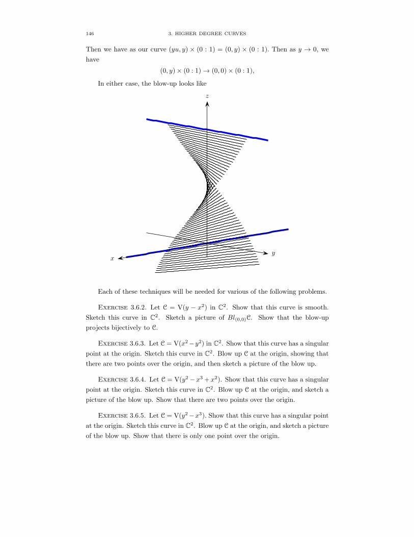
146 3. HIGHER DEGREE CURVES
Then we have as our curve (yu, y) × (0 : 1) = (0, y) × (0 : 1). Then as y → 0, we
have
(0, y)× (0 : 1) → (0, 0)× (0 : 1),
In either case, the blow-up looks like
xy
z
Each of these techniques will be needed for various of the following problems.
Exercise 3.6.2. Let C = V(y − x2) in C2. Show that this curve is smooth.
Sketch this curve in C2. Sketch a picture of Bl(0,0)C. Show that the blow-up
projects bijectively to C.
Exercise 3.6.3. Let C = V(x2−y2) in C2. Show that this curve has a singular
point at the origin. Sketch this curve in C2. Blow up C at the origin, showing that
there are two points over the origin, and then sketch a picture of the blow up.
Exercise 3.6.4. Let C = V(y2 − x3 + x2). Show that this curve has a singular
point at the origin. Sketch this curve in C2. Blow up C at the origin, and sketch a
picture of the blow up. Show that there are two points over the origin.
Exercise 3.6.5. Let C = V(y2−x3). Show that this curve has a singular point
at the origin. Sketch this curve in C2. Blow up C at the origin, and sketch a picture
of the blow up. Show that there is only one point over the origin.

3.6. BLOWING UP 147
Exercise 3.6.6. Let C = V((x − y)(x + y)(x + 2y)) be a curve in C2. Show
that this curve has a singular point at the origin. Sketch this curve in C2. Blow
up C at the origin, and sketch a picture of the blow up. Show that there are three
points over the origin.
The previous exercises should convey the idea that if the original curve is sin-
gular at the origin, then the blow-up seems to be less singular at its point over the
origin. We currently can’t express precisely what this means, since our definition
of singularity applies only to curves in the plane, and the blow-up does not lie in
a plane. Algebraic ideas developed in Chapter 4 will allow us to make this idea
precise.
Of course, there is nothing special about the origin in affine space, and we could
just as easily blow up curves at any other point. Also, the definition of blowing up
can easily be extended to curves in projective spaces. Blowing up will be discussed
in full generality in Chapter 4, once we have the necessary algebraic tools.


CHAPTER 4
Affine Varieties
The goal of this chapter is to start using more algebraic concepts to describe the
geometry of curves and surfaces in a fairly concrete setting. We will translate the
geometric features into the language of ring theory, which can then be extended to
encompass curves and surfaces defined over objects besides the real numbers or the
complex numbers. You will need to know some basic facts about rings, including
ideals, prime ideals, maximal ideals, sub-rings, quotient rings, ring homomorphisms,
ring isomorphisms, integral domains, fields, and local rings. Most undergraduate
abstract algebra texts include this material, and can be used as a reference. In
addition, some concepts from topology and multivariable calculus are needed. We
have tried to include just enough of these topics to be able to work the problems.
By considering the set of points where a polynomial vanishes, we can see there is
a correspondence between the algebraic concept of a polynomial and the geometric
concept of points in the space. This chapter is devoted to understanding that
connection. Here tools from abstract algebra, especially commutative ring theory,
will be become key.
Definition 4.0.1. For a field k, the affine n-space over k is the set
An(k) = (a1, a2, . . . , an) : ai ∈ k for i = 1, . . . , n.
We write simply An when the field k is understood.
For example, A2(R) is the familiar Euclidean space R2 from calculus, and A1(C)
is the complex line. We are interested in subsets of An that are the zero sets of a
collection of polynomials over k.
4.1. Zero Sets of Polynomials
Recall that k[x1, x2, . . . , xn] is the commutative ring of all polynomials in the
variables x1, x2, . . . , xn with coefficients in the field k. Frequently for us, our field
will be the complex numbers C, with the field of the real numbers R being our
second most common field.
149

150 4. AFFINE VARIETIES
4.1.1. Over C.
Exercise 4.1.1. Describe or sketch the zero set of each polynomial over C.
(1) x2 + 1(2) y − x2
Exercise 4.1.2. (1) Show that the zero set of x2 + y2 − 1 in C2 is un-
bounded. Contrast with the zero set of x2 + y2 − 1 in R2.
(2) Show that the zero set of any nonconstant polynomial in two variables
over C is unbounded.
Exercise 4.1.3. Find a set of polynomials P1, . . . , Pn, all of whose coeffi-
cients are real numbers, whose common zero set is the given set.
(1) (3, y) : y ∈ R in R2
(2) (1, 2) in R2
(3) (1, 2), (0, 5) in R2
(4) Generalize the method from part iii. to any finite set of points a1, . . . , anin R2.
Exercise 4.1.4. Find a set of polynomials P1, . . . , Pn, all of whose coeffi-
cients are complex numbers, whose common zero set is the given set.
(1) (3 + 2i,−i) in C2
(2) (3 + 2i,−i), (0, 1− 4i) in C2
(3) Generalize the method from part ii. to any finite set of points b1, . . . , bnin C2.
Exercise 4.1.5. (1) Is any finite subset of C2 the zero set of a polynomial
C[x, y]? Prove or find a counterexample.
(2) Is there an infinite subset of C2 that is the common zero set of a finite
collection of polynomials in C[x, y]?
(3) Find an infinite set of points in C that is not the common zero set of a
finite collection of polynomials in C[x]?
(4) Is there any infinite set of points in C, besides C itself, that is the common
zero set of a finite collection of polynomials in C[x]?
4.1.2. Over Z5. One of the great advantages of algebraic geometry is that we
may consider polynomials over any field. Our fields do not even need to be infinite!
We can define Z5 using an equivalence relation; a ≡ b if and only if a − b is a
multiple of 5. There are 5 elements in this field, we can call them 0, 1, 2, 3, and 4.
Addition and multiplication is defined by the usual operation followed by equating
the result with its representative from this set.
Exercise 4.1.6. Find the zero set of each polynomial in Z5.

4.2. ALGEBRAIC SETS 151
(1) x2 + 1
(2) x2 − 2
Exercise 4.1.7. Sketch the zero set of each polynomial in A2(Z5).
(1) y − x2
(2) y2 − 2xy + x2
(3) xy − 3y − x2 + 3x
4.1.3. Over Any Field k. Much of the reason that modern algebraic geome-
try heavily influences not just geometry but also number theory is that we can allow
our coefficients to be in any field, even those for which no geometry is immediately
apparent.
Exercise 4.1.8. (1) Show that if k is an infinite field, and P ∈ k[x1, . . . , xn]
is a polynomial whose zero set is An(k), then P = 0. Hint: Use induction
on n.
(2) Is there any finite field for which this result holds?
4.2. Algebraic Sets
The zero sets of polynomials in affine space are called algebraic sets.
Definition 4.2.1. Let S ⊆ k[x1, . . . , xn] be a set of polynomials over k. The
algebraic set defined by S is
V (S) = (a1, a2, . . . , an) ∈ An(k) : P (a1, a2, . . . , an) = 0 for all P ∈ S.
Exercise 4.2.1. Sketch the algebraic sets.
(1) V (x3 + 1) in A1(C)
(2) V ((y − x2)(y2 − x)) in A2(R)
(3) V (y − x2, y2 − x) in A2(R)
(4) V (y2 − x3 + x) in A2(R)
(5) V (x− 2y + 3z) in A3(R)
(6) V (z − 3, z − x2 − y2) in A3(R)
(7) V (xy − z2y) = V (y(x− z2)) in A3(R)
(8) V (y − x+ x2) in A2(Z3)
Exercise 4.2.2. Algebraic Sets in Rn and Cn:
(1) Show that for any a ∈ R, the singleton a is an algebraic set.
(2) Show that any finite collection of numbers a1, a2, . . . , ak in R is an
algebraic set.
(3) Show that a circle in R2 is an algebraic set.
(4) Show that the set (−1/√2, 1/
√2), (1/
√2,−1/
√2) ⊂ R2 is an algebraic
set.

152 4. AFFINE VARIETIES
(5) Show that any line in R3 is an algebraic set.
(6) Give an example of a subset of C2 that is not an algebraic set.
(7) Give an example of a nonconstant polynomial P in R[x, y] such that the
algebraic set X = (x, y) ∈ R2|P (x, y) = 0 is the empty set.
(8) Is there a nonconstant polynomial P in C[x, y] such that the algebraic set
X = (x, y) ∈ C2|P (x, y) = 0 is the empty set? Explain why or why not.
(9) Suppose X1 = (x, y) ∈ C2|x+ y = 0 and X1 = (x, y) ∈ C2|x− y = 0.Find a polynomial Q ∈ C[x, y] such that X1∪X2 = (x, y) ∈ C2|Q(x, y) =
0.(10) Suppose X1 = (x1, x2, . . . , xn) ∈ Cn|P1(x1, x2, . . . , xn) = 0 and X2 =
(x1, x2, . . . , xn) ∈ Cn|P2(x1, x2, . . . , xn) = 0. Give a single polynomial
Q such that X1 ∪X2 = (x1, x2, . . . , xn) ∈ Cn|Q(x1, x2, . . . , xn) = 0.
Exercise 4.2.3. (1) Is any finite subset of A2(R) an algebraic set?
(2) Is any finite subset of A2(C) an algebraic set?
Exercise 4.2.4. Show that the set (x, y) ∈ A2(R) :: 0 ≤ x ≤ 1, y = 0 is
not an algebraic set. (Hint: any one-variable polynomial, that is not the zero
polynomial, can only have a finite number of roots.)
Exercise 4.2.5. Show that the empty set and An(k) are algebraic sets in An(k).
Exercise 4.2.6. Show that if X = V (f1, . . . , fs) and W = V (g1, . . . , gt) are
algebraic sets in An(k), then X ∪W and X ∩W are algebraic sets in An(k).
4.3. Zero Sets via V (I)
The goal of this section is to start to see how ideals in rings give us algebraic sets.
Exercise 4.3.1. Let f(x, y), g(x, y) ∈ C[x, y]. Show that
V (f, g) = V (f − g, f + g).
Exercise 4.3.2. Show that V (x+y, x−y, 2x+y2, x+xy+y3, y+x2y) = V (x, y).
Thus the polynomials that define a zero set are far from being unique. But
there is an algebraic object that comes close to be uniquely linked to a zero set.
The following exercise is key to algebraic geometry.
Exercise 4.3.3. Let I be the ideal in k[x1, . . . , xn] generated by a set S ⊂k[x1, . . . , xn]. Show that V (S) = V (I). Thus every algebraic set is defined by an
ideal.
While it is not quite true that the set V (I) uniquely determines the ideal I, we
will soon see how to restrict our class of ideas so that the associated ideal will be
unique.

4.3. ZERO SETS VIA V (I) 153
Exercise 4.3.4. For f(x1, . . . , xn), g(x1, . . . , xn) ∈ C[x1, . . . , xn], let I be the
ideal generated by f and g and let J be the ideal generated by f alone.
(1) Show that J ⊂ I.
(2) Show that
V (I) ⊂ V (J).
Exercise 4.3.5. Show that if I and J are ideals in k[x1, . . . , xn] with I ⊂ J ,
then V (I) ⊃ V (J).
Exercise 4.3.6. You may find exercise 4.2.6 useful here.
(1) Show that an arbitrary intersection of algebraic sets is an algebraic set.
(2) Show that a finite union of algebraic sets is an algebraic set.
(3) Use your answers to parts a. and b. and exercise 4.2.5 to conclude that
the collection of complements of algebraic sets forms a topology on An(k).
4.3.1. Ideals Associated to Zero Sets. We have seen that the set of poly-
nomials that define a zero set is not unique. We need to find a structure derived
from these polynomials that is unique. At first glance, it looks like an ideal of the
polynomial ring would do the job. As we will see, not all ideals will work, but a
particular type of ideal is what we need.
Definition 4.3.1. Let V be a an algebraic set in An(k). The ideal of V is
given by
I(V ) = P ∈ k[x1, . . . , xn] : P (a1, . . . , an) = 0 for all (a1, . . . , an) ∈ V .
Similarly, for any set of points X in An(k), we define
I(X) = P ∈ k[x1, . . . , xn] : P (a1, . . . , an) = 0 for all (a1, . . . , an) ∈ X.
Exercise 4.3.7. Show that I(V ) is an ideal in the ring k[x1, . . . , xn].
Exercise 4.3.8. Let X be a set of points in An(k).
(1) Show that X ⊆ V (I(X)).
(2) Find a set X with X 6= V (I(X)).
(3) In part b., can you find a set X such that I(X) 6= 〈0〉?(4) Show that if X is a non-empty algebraic set, then X = V (I(X)).
Exercise 4.3.9. Let I be an ideal in k[x1, . . . , xn].
(1) Show that I ⊆ I(V (I)).
(2) Find an ideal I with I 6= I(V (I)).
(3) In part ii., can you find an ideal I such that V (I) 6= ∅?(4) Show that if I is the ideal given by an algebraic set, then I = I(V (I)).

154 4. AFFINE VARIETIES
It looks like there is a correspondence between algebraic sets and some ideals.
Let’s examine the properities of a good ideal a little more closely.
Definition 4.3.2. Let I be an ideal in k[x1, . . . , xn]. The radical of I is defined
as
Rad(I) = P ∈ k[x1, . . . , xn] : Pm ∈ I for some m > 0.
An ideal I is called a radical ideal if I = Rad(I).
Exercise 4.3.10. Let f(x, y) = (x2 − y + 3)2 ∈ C[x, y]. Show that the ideal I
generated by f is not radical. Find Rad(I).
Exercise 4.3.11. Let I be an ideal in k[x1, . . . , xn]. Show that Rad(I) is an
ideal.
Thus for any algebraic set X , there is the uniquely defined associated radical
ideal.
Exercise 4.3.12. Let X be a set of points in An(k). Show that I(X) is a
radical ideal.
Exercise 4.3.13. Show that Rad(I) ⊂ I(V (I)) for any ideal I in k[x1, . . . , xn].
Exercise 4.3.14. Let X and W be algebraic sets in An(k). Show that X ⊂W
if and only if I(X) ⊃ I(W ). Conclude that X =W if and only if I(X) = I(W ).
4.4. Functions on Zero Sets and the Coordinate Ring
One of the themes in 20th century mathematics is that it is not clear what
is more important in geometry: the actual geometric point set or the space of
functions defined on the geometric point set. So far in this chapter, we have been
concentrating on the point set. We now turn to the functions on the point sets.
Let V ⊆ An(k) be an algebraic set. Then it is very natural to consider the set
O(V ) := f : V → k | f is a polynomial function.
Exercise 4.4.1. Show that if we equip k[V ] with pointwise addition and mul-
tiplication of functions, then k[V ] is a ring. We will call k[V ] the coordinate ring
associated to V .
Given an algebraic set V , recall that by I(V ) we mean the vanishing ideal of
V , i.e. the ideal in k[x1, . . . , xn] consisting of polynomial functions f that satisfy
f(V ) = 0 for all x ∈ V .
Exercise 4.4.2. Let f(x, y) = x2 + y2 − 1 ∈ C[x, y]. Consider the two polyno-
mials g(x, y) = y, h(x, y) = x2 + y2 + y − 1.

4.5. HILBERT BASIS THEOREM 155
(1) Find a point (a, b) ∈ A2(C) such that
g(a, b) 6= h(a, b).
(2) Show for any point (a, b) ∈ V (f) that
g(a, b) = h(a, b).
Thus g and h are different as functions on A2(C) but should be viewed as equal on
algebraic set V (I).
Exercise 4.4.3. Let f(x, y) = x2+y2−1 ∈ C[x, y]. Suppose that g, h ∈ C[x, y]such that for all (a, b) ∈ V (f) we have g(a, b) = h(a, b). Show that the polynomial
g(x, y)− h(x, y) ∈< x2 + y2 − 1 > .
Exercise 4.4.4. Let V be an algebraic set in An(k). Prove that O(V ) is ring-
isomorphic to k[x1, . . . , xn]/I(V ). (Here we are using that two functions should be
viewed as equal if they agree on all points of the domain.)
Exercise 4.4.5. Let V ⊆ kn be an algebraic set. Prove that there is one-to-one
correspondence from the set of all ideals of k[x1, . . . , xn]/I(V ) onto the set of all
ideals of k[x1, . . . , xn] containing I(V ).
Exercise 4.4.6. Let V ⊆ kn and W ⊆ km be algebraic sets.
(1) Let f : V → W be a polynomial map, and define φ : k[W ] → k[V ] by
φ(g) = g f . Show that φ is a k-algebra homomorphism.
(2) Show that for each k-algebra homomorphism φ : k[W ] → k[V ] there exists
a polynomial map f : V → W such that φ(g) = g f , for all g ∈ k[W ].
4.5. Hilbert Basis Theorem
The goal of this section is prove the Hilbert Basis Theorem, which has as a conse-
quence that every ideal in C[x1, . . . , xn] is finitely generated.
How many polynomials are needed to define an algebraic set V ⊂ Cn? Is there
a finite number of polynomials f1, f2, . . . , fm such that
V = a ∈ Cn : fi(a) = 0, ∀ 1 ≤ i ≤ m,
or are there times that we would need an infinite number of defining polynomials?
Exercise 4.5.1. Let V = (x2 + y2 − 1 = 0). Show that I(V ) contains an
infinite number of elements.
We know that there are an infinite number of possible defining polynomials,
but do we need all of them to define V . In the above exercise, all we need is the
single x2 + y2 − 1 to define the entire algebraic set. If there are times when we

156 4. AFFINE VARIETIES
need an infinite number of defining polynomials, then algebraic geometry would be
extremely hard. Luckily, the Hilbert Basis Theorem has as its core that we only
need a finite set of polynomials to generate any ideal. The rest of this section will
be pure algebra.
Recall that a (commutative) ring R is said to be Noetherian if every ideal
I in R is finitely generated. (Recall that all rings considered in this book are
commutative.)
We will define a ring R to be noetherian if every ideal of R is finitely generated.
Exercise 4.5.2. Show that every field and every principal ideal domain are
Noetherian.
Exercise 4.5.3. Let R be a ring. Prove that the following three conditions are
equivalent:
(1) R is Noetherian.
(2) Every ascending chain I1 ⊆ I2 ⊆ · · · ⊆ In ⊆ · · · of ideals in R is stationary,
i.e., there exists N such that for all n ≥ N , In = IN .
(3) Every nonempty set of ideals in R has a maximal element (with inclusion
being the ordering between ideals).
In what follows, we guide the reader through a proof of the Hilbert Basis
Theorem.
Exercise 4.5.4. Consider the polynomial ring R[x], where R is a Noetherian
ring. If I ⊆ R[x] is an ideal and n ∈ N, let In be the set of leading coefficients of
elements of I of degree n. Prove that In is an ideal in R.
Exercise 4.5.5. Consider the polynomial ring R[X ], where R is a Noetherian
ring. Show that any ideal I ⊆ R[X ] is finitely generated.
The previous exercise establishes the following
Theorem 4.5.6 (Hilbert Basis Theorem). If R is a Noetherian ring then R[x]
is also a Noetherian ring.
Sketch of proof. Let I ⊂ R[x] be an ideal of R[x]. We show I is finitely generated.
Step 1. Let f1 be a nonzero element of least degree in I.
Step 2. For i > 1, let fi be an element of least degree in I \ f1, . . . , fi−1, ifpossible.
Step 3. For each i, write fi = aixdi + lower order terms. That is, let ai be the
leading coefficient of fi. Set J = (a1, a2, . . .).
Step 4. Since R is Noetherian, J = (a1, . . . , am) for some m.
Step 5. Claim that I = (f1, . . . , fm). If not, there is an fm+1, and we can subtract
off its leading term using elements of (f1, . . . , fm) to get a contradiction.

4.6. HILBERT NULLSTELLENSATZ 157
Exercise 4.5.7. Justify Step 4 in the above proof sketch.
Exercise 4.5.8. Fill in the details of Step 5.
Exercise 4.5.9. Show that if R is Noetherian then R[x1, . . . , xn] is Noetherian.
Definition 4.5.1. Loosely speaking, a formal power series is a power series
in which questions of convergence are ignored.
Definition 4.5.2. The set of all formal power series in variable x with coeffi-
cients in a commutative ring R form another ring that is written R[[X ]], and called
the ring of formal power series in the variable x over R.
Exercise 4.5.10. Let R be a Noetherian ring. Prove that the formal power
series ring R[[x]] is also Noetherian.
Exercise 4.5.11. Let R be a ring all of whose prime ideals are finitely gener-
ated. Prove that R is Noetherian.
4.6. Hilbert Nullstellensatz
The goal of this section is to guide the reader through a proof of Hilbert’s Null-
stellensatz. Hilbert’s Nullstellensatz show there is a one-to correspondence between
algebraic sets in Cn and radical ideals.
(This section is based on Arrondo’s “Another Elementary Proof of the Null-
stellensatz,” which appeared in the American Mathematical Monthly on February
of 2006.)
We know, given any ideal I ⊂ C[x1, x2, . . . , xn], that
V (I) = V (√I).
But can there be some other ideal J ⊂ C[x1, x2, . . . , xn], with V (J) = V (I) but√I 6=
√J? The punch line for this section is that this is impossible.
Exercise 4.6.1. Prove that there exist λ1, . . . , λ4 ∈ C such that the coefficient
of x24 in f(x1 + λ1x4, x2 + λ2x4x3 + λ3x4, x4) is nonzero, where f(x1, x2, x3, x4) =
x1x2 + x3x4.
Exercise 4.6.2. Let F be an infinite field and f be a nonconstant polynomial
in F [x1, . . . , xn] (with n ≥ 2). Prove that there exist λ1, . . . , λn in F such that the
coefficient of xdn in f(x1 + λ1xn, . . . , xn−1 + λn−1xn, xn) is nonzero, whenever d is
the total degree of f(x1 + λ1xn, . . . , xn−1 + λn−1xn, xn).
158 4. AFFINE VARIETIES
Exercise 4.6.3. Let I ⊂ C[x1, . . . , x4] be an ideal containing the polynomial
f(x1, x2, x3, x4) = x1x2 + x3x4. Prove that, up to a change of coordinates and
scaling, I contains a polynomial g monic in the variable x4. (By monic, we mean
that the coefficient of the highest power for xn is one.)
Exercise 4.6.4. Let I be a proper ideal of F [x1, . . . , xn]. Prove that, up to a
change of coordinates and scaling, I contains a polynomial g monic in the variable
xn.
Exercise 4.6.5. Let I be a proper ideal of F [x1, . . . , xn] and let I ′ be the set
of all polynomials in I that do not contain the indeterminate xn. Prove that I ′ is
an ideal of F [x1, . . . , xn−1] and that, modulo a change of coordinates and scaling
(as in the previous exercise), the ideal I ′ is a proper ideal.
Exercise 4.6.6. Let I be an ideal of F [x1, . . . , xn] and let g ∈ I be a polynomial
monic in the variable xn. Suppose there exists f ∈ I such that f(a1, . . . , an−1, xn) =
1. Consider Res(f, g;xn) be the resultant of f and g with respect to the variable
xn, (refer to Definition 3.3.3) where f = f0 + f1xn + · · · + fdxdn with all the fi in
F [x1, . . . , xn−1] so that f0(a1, . . . , an−1) = 1 and fi(a1, . . . , an−1) = 0 for 1 ≤ i ≤ n,
and g = g0 + g1xn + · · · ge−1xe−1n + 1 · xen with all the gj in F [x1, . . . , xn−1]. Show
that (under the current faulty hypotheses)
(1) R ∈ I;
(2) R ∈ I ′;
(3) R(a1, . . . , an−1) = 1.
Exercise 4.6.7. Let I be a proper ideal of F [x1, . . . , xn]. Prove that, modulo
a change of coordinates and scaling, the set
J := f(a1, . . . , an−1, xn) | f ∈ I
is a proper ideal of F [xn].
Exercise 4.6.8. Let I be a proper ideal of F [x1, . . . , xn]. Prove that if F is
algebraically closed, then there exists (a1, . . . , an) in Fn such that f(a1, . . . , an) = 0
for all f ∈ I.
Exercise 4.6.9 (Weak Nullstellensatz). Let F be an algebraically closed field.
Then an ideal I in F [x1, . . . , xn] is maximal if and only if there are elements ai ∈ F
such that I is the ideal generated by the elements xi − ai; that is I = 〈x1 −a1, . . . , xn − an〉.
Recall that an ideal I of a ring R is said to be a radical ideal if xn ∈ I for some
n ≥ 1 implies that x ∈ I. Given an arbitrary ideal I of a ring R, the radical√I of
I is the set of all elements x ∈ R such that some positive power of x is in I.
4.7. VARIETY AS IRREDUCIBLE ALGEBRAIC SET: PRIME IDEALS 159
Exercise 4.6.10. Given a ring R and an ideal I of R, prove that the radical√I of I is an ideal.
Exercise 4.6.11. Let F be a field, and let V be an algebraic set in Fn for
some n ≥ 1. Prove that I(V ) is a radical ideal in the polynomial ring F [x1, . . . , xn].
Moreover, prove that V (I(V )) = A for any algebraic set A. (By V (I) we mean the
vanishing set of I.)
Exercise 4.6.12. Give an example where√I I(V (
√I)), where V (J) denotes
the vanishing set of J .
Exercise 4.6.13 (Strong Nullstellensatz). Let F be an algebraically closed field
and let I be an ideal of the polynomial ring F [x1, . . . , xn]. Then I(V (I)) =√I.
4.7. Variety as Irreducible Algebraic Set: Prime Ideals
The goal of this section is to define affine varieties and to explore their topology
and coordinate rings.
4.7.1. Irreducible components.
Definition 4.7.1. An algebraic set V is reducible if V = V1 ∪ V2, where V1and V2 are algebraic sets with V1 ( V and V2 ( V . An algebraic set that is not
reducible is said to be irreducible.
Definition 4.7.2. An affine variety is an irreducible algebraic set.
Exercise 4.7.1. Show that A1 is irreducible, so A1 is an affine variety.
Exercise 4.7.2. Decide if the following algebraic sets in A2 are reducible or
irreducible.
(1) V (x)
(2) V (x+ y)
(3) V (xy)
Exercise 4.7.3. Let f ∈ k[x, y] and set V = V (f). Show that if f factors as a
product f = gh of nonconstant polynomials g, h ∈ k[x, y], then V is reducible.
4.7.2. Prime and non-prime ideals.
Definition 4.7.3. A proper ideal I ⊂ R is a prime ideal in R if, whenever
ab ∈ I for a, b ∈ R, either a ∈ I or b ∈ I (or both).
Definition 4.7.4. A proper ideal I ⊂ R is a maximal ideal in R if I ( J ⊂ R
for some ideal J implies that J = R.

160 4. AFFINE VARIETIES
Exercise 4.7.4. Every ideal I in Z is of the form I = 〈m〉 for some m ∈ Z.(1) For what values of m is the ideal I = 〈m〉 a prime ideal in Z.
(2) For what values of m is the ideal I = 〈m〉 a maximal ideal in Z.
Exercise 4.7.5. Let f(x, y) = xy ∈ k[x, y]. Show that the ideal 〈f〉 is not a
prime ideal.
Exercise 4.7.6. Let f ∈ k[x] be a nonconstant polynomial. Prove that f is
an irreducible polynomial if and only if 〈f〉 is a prime ideal.
Exercise 4.7.7. Let I be an ideal in a ring R.
(1) Show that I ⊂ R is a prime ideal if and only if R/I is an integral domain.
(2) Show that I ⊂ R is a maximal ideal if and only if R/I is a field.
(3) Explain why every maximal ideal in R is prime.
Exercise 4.7.8. Let I be an ideal in a ring R. Show that√I =
⋂
prime p⊇I
p,
where Rad(I) = a ∈ R : an ∈ I for some n > 0.
Exercise 4.7.9. Let ϕ : R → S be a ring homomorphism.
(1) Let J ⊂ S be a prime ideal in S. Show that ϕ−1(J) is a prime ideal in R.
(2) Let J ⊂ S be a maximal ideal in S. Is ϕ−1(J) a maximal ideal in R?
Prove or find a counterexample.
4.7.3. Varieties and Prime Ideals. We now reach the key results of this
section.
Exercise 4.7.10. Let V ⊂ An be an algebraic set.
(1) Suppose that V is reducible, say V = V1∪V2 where V1 and V2 are algebraicsets with V1 ( V and V2 ( V . Show that there are polynomials P1 ∈ I(V1)
and P2 ∈ I(V2) such that P1P2 ∈ I(V ) but P1, P2 6∈ I(V ). Conclude that
I(V ) is not a prime ideal.
(2) Prove that if I(V ) is not a prime ideal in k[x1, . . . , xn], then V is a re-
ducible algebraic set.
is a prime ideal.
Exercise 4.7.11. Let V be an algebraic set in An. Prove that the following
are equivalent:
(1) V is an affine variety.
(2) I(V ) is a prime ideal in k[x1, . . . , xn].
(3) The coordinate ring, O(V ), of V is an integral domain.

4.8. SUBVARIETIES 161
Exercise 4.7.12. Let C be the collection of nonempty algebraic sets in An that
cannot be written as the union of finitely many irreducible algebraic sets.
(1) Suppose C is not empty. Show that there is an algebraic set V0 in C such
that V0 does not contain any other set in C. [Hint: If not, construct an
infinite descending chain of algebraic sets V1 ⊃ V2 ⊃ · · · in An. This
implies I(V1) ⊂ I(V2) ⊂ · · · is an infinite ascending chain of ideals in
k[x1, . . . , xn]. Why is this a contradiction?]
(2) Show that the result of part (1) leads to a contradiction, so our assumption
that C is not empty was false. Conclude that every algebraic set in An
can be written as a union of a finite number of irreducible algebraic sets
in An.
(3) Let V be an algebraic set in An. Show that V can be written as a union
of finitely many irreducible algebraic sets in An, V = V1 ∪ · · · ∪ Vk, suchthat no Vi contains any Vj .
(4) Suppose that V1∪· · ·∪Vk =W1∪· · ·∪W`, where the Vi,Wj are irreducible
algebraic sets in An such that no Vi contains any Vj and no Wi contains
any Wj if i 6= j. Show that k = ` and, after rearranging the order,
V1 =W1, . . . , Vk =Wk.
Therefore, every algebraic set in An can be expressed uniquely as the union of
finitely many affine varieties, no one containing another.
4.7.4. Examples.
Exercise 4.7.13. Show that An is an irreducible algebraic set for every n ≥ 1.
Thus every affine space is an affine variety.
Exercise 4.7.14. Let f ∈ k[x, y] be an irreducible polynomial. Show that
V (f), which is a curve in A2, is an irreducible algebraic set.
4.8. Subvarieties
The goal of this section is to define subvarieties and see how some of their ideal
theoretic properties.
Definition 4.8.1. Let W be an algebraic variety that is properly contained in
an algebraic variety V ⊂ An(k). Then W is a subvariety of V .
Exercise 4.8.1. Let V = (x− y = 0) ⊂ A2(C). Show that the point p = (1, 1)
is a subvariety of V , while the point q = (1, 2) is not a subvariety of V .

162 4. AFFINE VARIETIES
Exercise 4.8.2. Still using the notation from the first problem, show that
I(V ) is contained in an infinite number of distinct prime ideals. Give a geometric
interpretation for this.
Exercise 4.8.3. From the previous problem, find I(V ), I(p) and I(q). Show
that
I(V ) ⊂ I(p)
and
I(V ) 6⊂ I(q).
Exercise 4.8.4. Let W be a subvariety of V . Show that
I(V ) ⊂ I(W ).
Exercise 4.8.5. Let V and W be two algebraic varieties in An(k). Suppose
that
I(V ) ⊂ I(J).
Show that W is a subvariety of V .
Thus we have an elegant diagram:
W ⊂ V
I(W ) ⊃ I(V )
We now want to explore the relation between the coordinate ring O(V ) and
any coordinate ring O(W ) for any subvariety W of a variety V .
Exercise 4.8.6. Continue letting V = (x − y = 0) ⊂ A2(C), with subvariety
p = (1, 1). Find a polynomial f ∈ C[x, y] that is not identically zero on points of V
but is zero at p, meaning there is a point q ∈ V with f(q) 6= 0 but f(p) = 0. Show
that√
(f, I) = J,
where I = I(V ) and J = I(p). (Hint: if you choose f reasonably, then the ideal
(f, I) will itself be equal to the ideal J .)
We have to worry a bit about notation. For V ⊂ An(k), we know that
O(V ) = k[x1, . . . , xn]/I(V ). Then given any f ∈ k[x1, . . . , xn], we can think of
f as a function on V and hence as an element of O, but we must keep in mind that
if we write f ∈ O, then f is standing for the equivalence class f + I, capturing that
if f and g ∈ k[x1, . . . , xn]/I(V ) agree on all points of V , the f − g ∈ I and hence
f + I = g + I, representing the same function in O.
We have a ring theoretic exercise first.

4.9. FUNCTION FIELDS 163
Exercise 4.8.7. Let R be a commutative ring. Let I ⊂ J be two ideals in R.
Show that J/I is an ideal in the quotient ring R/I. Show that there is a natural
onto map
R/I → R/J
whose quotient is the ideal J/I.
Exercise 4.8.8. Continue letting V = (x − y = 0) ⊂ A2(C), with subvariety
p = (1, 1). Explicitly check the above exercise for R = C[x, y], I = (V ) and J =
I(p).
For any type of subsets W ⊂ V , if f : V → k, then there is the natural
restriction map f |W :W → k, which just means for all p ∈W that we define
f |W (p) = f(p).
Exercise 4.8.9. Let W be a subvariety of a variety V ⊂ An(k). Let f ∈ O(V ).
Show that the above restriction map sends f to an element of O(W ) and that this
restriction map is a ring homomorphism.
Exercise 4.8.10. Show that the kernel of the above restriction map is I(W )/I(V )
in the ring O(V ).
Exercise 4.8.11. Discuss why each subvariety W of V should correspond to
an onto ring homomorphism from the coordinate ring O(V ) to a commutative ring.
Thus there are three equivalent ways for thinking of subvarieties of an algebraic
variety V :
(1) W as an algebraic variety probably contained in an algebraic variety V .
(2) A prime ideal J properly containing the prime ideal I(V )
(3) A quotient ring of the ring O(V ) = k[x1, . . . , xn]/I(V ).
4.9. Function Fields
The goal of this section is to associate not just a ring to an algebraic variety but
also a field. This field plays a critical role throughout algebraic geometry.
Every algebraic variety V corresponds to a prime ideal I ⊂ C[x1, . . . , xn]. Thisallowed us to define the ring of functions on V , namely the quotient ring OV =
C[x1, . . . , xn]/I. But every commutative ring sits inside of a field, much like the
integers can be used to define the rational numbers. The goal of this subsection is
to define the function field KV , which is the smallest field that the quotient ring
OV lives in.

164 4. AFFINE VARIETIES
Definition 4.9.1. Given an algebraic variety V corresponding to a prime ideal
I ⊂ C[x1, . . . , xn], the function field KV is:
KV =
f
g: f, g ∈ OV /
(f1g1
=f2g2
)
where f1g1
= f2g2
means that
f1g2 − f2g1 ∈ I.
So far, KV is simply a set. To make it into a field, we need to define how to
add and multiply its elements. Define addition to be:
e
f+g
h=eh+ fg
fh
and multiplication to bee
f· gh=eg
fh.
Exercise 4.9.1. Show that addition is well-defined. This means you must
show that ife1f1
=e2f2,g1h1
=g2h2,
thene1h1 + f1g1
f1h1=e2h2 + f2g2
f2h2.
Exercise 4.9.2. Show that multiplication is well-defined. This means you
must show that ife1f1
=e2f2,g1h1
=g2h2,
thene1g1f1h1
=e2g2f2h2
.
Under these definitions, KV is indeed a field.
Often a slightly different notation used. Just as C[x1, . . . , xn] denotes the ring
of all polynomials with complex coefficients and variables x1, . . . xn, we let
C(x1, . . . , xn) =
f
g: f, g ∈ C[x1, . . . , xn]
subject to the natural relation that f1g1
= f2g2
means that f1g2 − f2g1 = 0. Then we
could have defined the function field of a variety V = V (I) to be
KV =
f
g: f, g ∈ C[x1, . . . , xn]
/I.
4.11. THE ZARISKI TOPOLOGY 165
4.10. Points as Maximal Ideals
Definition 4.10.1. Let R be a ring. Recall that an ideal I ⊂ R is maximal if
I is proper (I 6= R) and any ideal J that contains I is either I or all of R.
Exercise 4.10.1. Show that for a1, a2, . . . , an ∈ k, the ideal I ⊂ k[x1, . . . , xn]
defined as
I = 〈x1 − a1, . . . xn − an〉is maximal.
[Hint: Suppose J is an ideal with I ( J , and show that J contains 1.]
Exercise 4.10.2. Show that if an ideal I ⊂ k[x1, . . . , xn] is maximal, then V (I)
is either a point or empty.
Exercise 4.10.3. Show that I((a1, . . . , an)) = 〈x1 − a1, . . . , xn − an〉.
Exercise 4.10.4. Show that if k is an algebraically closed field, then every
maximal ideal in k[x1, . . . , xn] can be defined as
I = 〈x1 − a1, . . . xn − an〉.
[Hint: Theorem 4.6.9.]
Exercise 4.10.5. Show that the result of the previous exercise is actually
equivalent to Hilbert’s Weak Nullstellensatz.
Combining Exercises 4.10.1 and 4.10.4, we obtain the following important fact.
Theorem 4.10.6. In an algebraically closed field k, there is a one-to-one cor-
respondence between points of An(k) and maximal ideals of k[x1, . . . , xn].
Exercise 4.10.7. Find a maximal ideal I ⊂ R[x1, . . . , xn] for which V (I) = ∅.
4.11. The Zariski Topology
The goal of this section is to show that there is an algebraically defined topology
for any ring.
4.11.1. Topologies. The development of topology is one of the great success
stories of early 20th century mathematics. With a sharp definition for a topolog-
ical space, once tricky notions such as “continuity” and “dimension” would have
rigorous, meaningful definitions. As with most good abstractions, these definitions
could be applied to situations far removed from what their founders intended. This
is certainly the case in algebraic geometry.
The goal of this subsection is to briefly review what it means for a set to have
a topology, using the standard topology on R and on Cn as motivating examples.
We start with the definition of a topology on a set X .

166 4. AFFINE VARIETIES
Definition 4.11.1. A topology on the set X is given by specifying a collection
U of subsets of X having the properties:
(1) Both the empty set and the entire set X are elements of the collection U.
(2) The union of any subsets of X in U is also in U. (It is critical that we
allow even infinite unions.)
(3) The finite intersection of any subsets of X in U is also in U. (Here is it
critical that we only allow finite intersections.)
A set U ∈ U is said to be open. A set C is said to be closed if its complement X−Cis open.
Let us look at a few examples.
Start with the real numbers R. We need to define what subsets will make up
the collection U.
Definition 4.11.2. A set U ⊂ R is a standard open set in R if for any a ∈ U ,
there exists an ε > 0 such that
x ∈ R : |x− a| < ε ⊂ U.
R U
(a− ε
•a
)a+ ε
Exercise 4.11.1. Let a, b ∈ R with a < b.
(1) Show that in R, (a, b) = x ∈ R : a < x < b is open.
(2) Show that in R, [a, b] = x ∈ R : a ≤ x ≤ b is closed.
(3) Show that in R, [a, b) = x ∈ R : a ≤ x < b is neither open nor closed.
(This type of set is often said to be half-open.)
Exercise 4.11.2. Show that the collection of standard open sets in R defines
a topology on R. This is called the standard topology on R.
Let us now put a topology on Cn.
Definition 4.11.3. A set U ⊂ Cn is a standard open set in Cn if for any a ∈ U ,
there exists an ε > 0 such that
x ∈ Cn : |x− a| < ε ⊂ U.
(Note that |x − a| =√|x1 − a1|2 + · · ·+ |xn − an|2 for a = (a1, . . . , an) and x =
(x1, . . . xn).)
Thus a set U is open in Cn if any of its points can be made the center of a little
open ball that lies entirely within U .

4.11. THE ZARISKI TOPOLOGY 167
Exercise 4.11.3. Show that the collection of standard open sets in Cn defines
a topology on Cn. This is called the standard topology on Cn.
Exercise 4.11.4. In C2, show that C2 −V(x2 + y2 − 1) is open.
Exercise 4.11.5. In C2, show that C2 − V(P ) is open for any polynomial
P (x, y).
Exercise 4.11.6. In C3, show that C3 −V(x2 + y2 + z2 − 1) is open.
Exercise 4.11.7. In Cn, show that Cn − V(P ) is open for any polynomial
P (x1, x2, . . . , xn), so V(P ) is closed in the standard topology on Cn.
Exercise 4.11.8. In C2, show that (x, y) ∈ C2 : |x|2 + |y|2 < 1 is open.
The standard topologies on R and Cn may be familiar to you. However, these
are not the only topologies that can be defined on these sets. In the next exercise
you will explore the finite complement topology on R and will see that it is different
than the standard topology.
Exercise 4.11.9. Finite complement topology on R: On R a set U is open if
the complement of U is a finite collection of points, i.e. U = R − p1, . . . , pk. Rand ∅ are also considered to be open sets.
(1) Verify that any arbitrary union of open sets is again open.
(2) Verify that any finite intersection of open sets is open.
(3) Conclude that the open sets defined above form a topology on R. This is
called the finite complement topology on R.
(4) Show that if a set U is open in the finite complement topology, then it is
open in the standard topology on R.
(5) Give an example of an open set in the standard topology on R that is not
open in the finite complement topology.
(6) Show that any two nonempty open sets in the finite complement topology
on R must intersect. Is the same true in the standard topology on R?
The final part of the previous exercise implies that the finite complement topol-
ogy on R is not “Hausdorff” while the standard topology is. In a Hausdorff topology
U on a set X , for any pair of distinct points p, q ∈ X you can find open sets U, V
such that p ∈ U , q ∈ V and U ∩ V = ∅. That is, we can “separate” p and q in X
with disjoint open sets from U. This is usually a desirable property in the study of
topology, but it is not a property of the topology we use in algebraic geometry, the
Zariski topology.

168 4. AFFINE VARIETIES
4.11.2. The Zariski Topology on An(k).
Definition 4.11.4. Let k be a field. A set X ⊂ An(k) is a Zariski-closed set
if X is an algebraic set. A set U is Zariski-open if U = An(k) −X where X is an
algebraic set.
Exercise 4.11.10.
(1) Use Exercises 4.2.5 and ?? to show that the collection of Zariski-open sets
in An(k) is a topology. This is called the Zariski topology on An(k).
(2) Show that a finite collection of points in An(k) is a Zariski-closed set.
Exercise 4.11.11. In this exercise, we compare the Zariski and finite comple-
ment topologies.
(1) Show that if a set U is open in the finite complement topology on An(k),
then it is open in the Zariski topology on An(k).
(2) Show that the finite complement topology on R is the same as the Zariski
topology on R.
(3) Show that the finite complement topology on C is the same as the Zariski
topology on C.
(4) Show that a circle in R2 is a Zariski-closed set. Conclude that the Zariski
topology is not the same as the finite complement topology on R2.
Exercise 4.11.12. In this exercise we describe the Zariski topology on C2.
(1) Show that, in C2, the complement of a finite number of points and alge-
braic curves is Zariski-open.
(2) Show that a non-empty Zariski-open set in C2 is the complement of a
finite number of points and algebraic curves.
Exercise 4.11.13. Show geometrically that the Zariski topology on C2 is not
Hausdorff.
4.11.3. Spec(R). For the standard topology on Cn it is critical that Cn has
a natural notion of distance. For fields like Z5, there is no such distance. Luckily
there is still a topology that we can associate to this or any other ring. The goal
of this subsection is to define the Zariski topology for any ring R.
We first have to specify our set of points. We will see that our “points” will
be the prime ideals in R. Recall that a proper ideal I in a ring R is prime if the
following holds: whenever f, g ∈ R with fg ∈ I, then f ∈ I or g ∈ I. A proper
ideal I of R is maximal if I ⊂ J for some ideal J in R implies that either J = I or
J = R.
Definition 4.11.5. The prime spectrum or spectrum of a ring R is the collec-
tion of prime ideals in R, denoted by Spec(R).

4.11. THE ZARISKI TOPOLOGY 169
Thus for any ring R, the set on which we will define our topology is Spec(R).
This definition should be seen as a generalization of Theorem ??, where we learned
that points of An(k) correspond to maximal ideals in k[x1, . . . , xn]. Since maximal
ideals are prime, the set Spec(R) includes all points from before and potentially
more as we explore in the following exercises.
Exercise 4.11.14. Describe the following sets.
(1) Spec(Z)
(2) Spec(R)
(3) Spec(k) for any field k
Exercise 4.11.15. Consider the polynomial ring C[x].
(1) Show that the ideal 〈0〉 is a prime ideal in C[x].
(2) Show that all prime ideals in C[x] are maximal ideals, except for the ideal
〈0〉.(3) Show for each point a ∈ C there is a corresponding prime ideal.
(4) Explain why Spec(C[x]) can reasonably be identified with C.
Exercise 4.11.16. Show that there are three types of points in Spec(R[x]):
i. The zero ideal 〈0〉,ii. Ideals of the form 〈x− a〉 for a real number a,
iii. Ideals of the form 〈x2 + a〉 for positive real numbers a.
Exercise 4.11.17. A curious property of “points” in Spec(R).
(1) Show that 〈x − y〉 is a prime ideal in C[x, y] and hence is a point in
Spec(C[x, y]).
(2) For two fixed complex numbers a and b, show that 〈x − a, y − b〉 is a
maximal ideal of C[x, y] and is hence also a point in Spec(C[x, y]).
(3) Show that for every a ∈ C, 〈x− a, y − a〉 contains the ideal 〈x − y〉.
Thus, in Spec(R), some “points” can be contained in others. This suggests
that not all points in Spec(R) are created equal. Returning to our motivation in
Theorem ??, we make the following definition.
Definition 4.11.6. The geometric points in Spec(R) are the maximal ideals.
By part (2) of Exercise 4.11.17, 〈x − a, y − b〉 is a maximal ideal in C[x, y],
and hence a geometric point in Spec(C[x, y]). In general, by Exercise 4.10.4,
the maximal ideals in C[x1, . . . , xn] are of the form 〈x1 − a1, . . . , xn − an〉 for
(a1, . . . , an) ∈ Cn. Thus the set of geometric points of Spec(C[x1, . . . , xn]) cor-
responds exactly to the set of points of Cn. However, we should not confuse these

170 4. AFFINE VARIETIES
two sets, for Spec(C[x1, . . . , xn]) contains many points other than its geometric ones
as indicated in the previous exercises.
Now that we are better acquainted with our set of points, we are ready to define
the topology.
Definition 4.11.7. Let S ⊆ R. Define the Zariski closed set given by S in
Spec(R) to be
Z(S) = P ∈ Spec(R) : P ⊇ S.A subset U of Spec(R) is Zariski open if there is a set S ⊆ R with
U = Spec(R)− Z(S).
Exercise 4.11.18. Let R be a ring. For a subset S of R, recall that 〈S〉 denotesthe ideal in R generated by S.
(1) For a set S ⊆ R, show that Z(S) = Z(〈S〉).(2) Show that Z(0) = Spec(R), and Z(1) = ∅.
Exercise 4.11.19. Show that a point I in Spec(R) is Zariski closed if and only
if the ideal I is maximal in R.
Thus the geometric points of Spec(R) coincide with the points of Spec(R) that
are Zariski closed. Thus we could have defined a geometric point as a point of
Spec(R) that is Zariski closed.
As in Section ?? we want to create a dictionary for going back and forth between
Zariski closed sets in Spec(R) and ideals in R. We have already described Z(S),
which assigns closed subsets of Spec(R) to ideals in R. Now we define the ideal
associated to a subset of Spec(R).
Definition 4.11.8. For X ⊆ Spec(R), define the ideal of X to be
I(X) =⋂
P∈X
P.
By Exercise 4.7.8 part (2), I(X) is a radical ideal in R.
Exercise 4.11.20. Let X and Y be subsets of Spec(R).
(1) Show that X ⊆ Z(I(X)).
(2) Show that if X ⊆ Y , then I(Y ) ⊆ I(X).
Exercise 4.11.21. Show that if X is a Zariski closed set in Spec(R), then
X = Z(I(X)).
Definition 4.11.9. For a subset Y of Spec(R), its Zariski closure of Y in
Spec(R) is Y = Z(I(Y )).
Exercise 4.11.22. Compute the Zariski closure of the following sets.

4.11. THE ZARISKI TOPOLOGY 171
(1) 〈2〉, 〈3〉 in Spec(Z)
(2) 〈0〉 in Spec(Z)
(3) 〈x− y〉 in Spec(C[x, y])
This reinforces our previous result that the geometric points of Spec(R) coincide
with the Zariski closed points. Part (2) is especially interesting and deserves a name.
Definition 4.11.10. A point of Spec(R) whose closure is the whole space is
called a generic point .
As we have already noted, the nature of points in Spec(R) challenges our geo-
metric intuition. Still, we have also seen that several of the results from Section ??
for our dictionary between closed sets and ideals in R continue to hold in Spec(R).
Here is one more of these results, which will prove important in our proof that the
collection of Zariski open sets defines a topology on Spec(R).
Exercise 4.11.23. Show that if X and Y are Zariski closed sets in Spec(R),
then X ∪ Y = Z(I(X) ∩ I(Y )) and X ∩ Y = Z(I(X) + I(Y )).
Exercise 4.11.24. Show that the Zariski closed sets are closed under arbitrary
intersections.
We want to show that the Zariski open sets make up a topology on Spec(R).
We first do a few set-theoretic exercises.
Exercise 4.11.25. Let X be a set. Define for any set U in X its complement
to be U c = X − U. Show that
(U c)c = U.
Exercise 4.11.26. For subsets Uα, α ∈ A, of a set X , let Cα = U cα.
(1) Show that ⋃
α
Uα = X −⋂
α
Cα.
(2) Show that ⋂
α
Uα = X −⋃
α
Cα.
With these results from set theory in hand, we return to the space Spec(R) and
prove that the collection of Zariski open sets defines a topology on this set.
Exercise 4.11.27. Let U1 and U2 be Zariski open sets in Spec(R). Show that
U1 ∩ U2 is a Zariski open set in Spec(R).
Exercise 4.11.28. Let Uα : α ∈ A be an arbitrary collection of Zariski open
sets in Spec(R). Show that⋃α Uα is a Zariski open set in Spec(R).
Exercise 4.11.29. Show that the collection of Zariski open sets forms a topol-
ogy on Spec(R).

172 4. AFFINE VARIETIES
4.12. Points and Local Rings
The goal of this section is to show how to link points on an algebraic variety V
with local rings of O(V ), which are subrings of the function field KV .
We want to study what is going on around a point p in an algebraic variety.
One approach would be to understand the behavior of the functions on V near p.
If we just want to know what is going on at p, then what a function is doing far
from p is irrelevant. The correct ring-theoretic concept will be that of a local ring.
We start with points in affine varieties V ⊂ An(k) and their local rings. We
then see how to put this into a much more general language.
4.12.1. Points as Maximal Ideals in Affine Varieties. In Section ?? we
proved that points in An(k) correspond to maximal ideals in k[x1, . . . , xn] and,
conversely, that maximal ideals correspond to points when the field k is algebraically
closed (Theorem ??). In the following exercises, we prove similar results for affine
varieties V ⊂ An(k).
Exercise 4.12.1. Let V = V(x2 + y2 − 1) ⊂ A2(k). Let p = (1, 0) ∈ V . Define
Mp = f ∈ O(V ) : f(p) = 0.
(1) Show that Mp is an ideal in O(V ).
(2) Show that Mp is in fact a maximal ideal in O(V ).
Exercise 4.12.2. Let M be a maximal ideal in O(V ) for the variety V =
V(x2 + y2 − 1) from the previous problem. Let
V(M) = p ∈ V : for all f ∈ M, f(p) = 0.
Show that V(M) must be a single point on V .
Exercise 4.12.3. Let V ⊂ An(k) be an algebraic variety. Let p be a point in
V . Define
Mp = f ∈ O(V ) : f(p) = 0.Show that Mp is a maximal ideal in O(V ) .
Exercise 4.12.4. Let M be a maximal ideal in O(V ), for V ⊂ An(k). Let
V (M) = p ∈ V : for all f ∈ M, f(p) = 0.
Show that V (M) must be a single point in V .
Thus we can either think of a point p as defining a maximal ideal in the co-
ordinate ring O(V ) or as a maximal ideal in O(V ) as defining a point on V . This
extends the results of Theorem ?? to affine varieties in general.

4.12. POINTS AND LOCAL RINGS 173
4.12.2. Local Ring at a Point. Let V ⊂ An(k) be an algebraic variety and
let p be a point in V . We want to concentrate on the functions on V defined near
p. Suppose there is a g ∈ O(V ) with g(p) 6= 0, say g(p) = 1. Then close to p,
whatever that means, the function g looks a lot like the constant function 1. This
means that we should be allowed to look at 1/g, which is generally not allowed in
O(V ) but is in its function field, KV .
Recall the construction of KV from Section ??. By definition,
KV =
f
g: f, g ∈ O(V ), g 6= 0
/
(f1g1
∼ f2g2
),
where f1/g1 ∼ f2/g2 if f1g2 − f2g1 ∈ I(V ). Addition and multiplication were
defined as usual for fractions,
f1g1
+f2g2
=f1g2 + f2g1
g1g2and
f1g1
· f2g2
=f1f2g1g2
,
both of which are well-defined. This set with these operations is then a field. We
now define the local ring at p to be a subring of this field.
Definition 4.12.1. Let p be a point on an algebraic variety V . The local ring
associated to p is
Op(V ) =
f
g∈ KV : g(p) 6= 0
.
Exercise 4.12.5. Let p be a point in an algebraic variety V . Prove that its
local ring Op(V ) is a subring of the function field KV .
Exercise 4.12.6. Let V = V(x2 + y2 − 1) ⊂ A2(k) and p = (1, 0) ∈ V .
(1) Show for f(x, y) = x ∈ Op(V ) that there is an element g ∈ Op(V ) such
that f · g = 1 in Op(V ).
(2) Show for f(x, y) = y ∈ Op(V ) that there can exist no element g ∈ Op(V )
such that f · g = 1 in Op(V ).
(3) Show that the ring Op(V ) cannot be a field.
Exercise 4.12.7. Let p be a point in an algebraic variety V ⊆ An(k) and let
Mp = f ∈ Op(V ) : f(p) = 0.
(1) Suppose that f 6∈ Mp. Show that there exists an element g ∈ Op(V ) such
that f · g = 1 in Op(V ).
(2) Show that Mp is the unique maximal ideal in the ring Op(V ).
4.12.3. Local Rings in Commutative Algebra. We now shift gears and
make things quite a bit more abstract. Part of the power of algebraic geometry
is that we can start with geometric insights and translate these into the language
of ring theory, allowing us to think geometrically about rings for which there is

174 4. AFFINE VARIETIES
little apparent geometry. This is not our emphasis in this book, but the following
is included to give just a flavor of this.
In Exercise 4.12.7 we saw that the local ring at a point p in an affine variety V ,
Op(V ), has a unique maximal ideal, Mp. Inspired by this, we make the following
definition for commutative rings in general.
Definition 4.12.2. A local ring is a ring that has a unique maximal ideal.
Now we can talk about local rings quite generally. For example, every field is
a local ring since the only proper ideal in a field is the zero ideal. However, as we
have seen in Exercise 4.12.6, not every local ring is a field.
The rest of this section develops the method of localization for creating local
rings from a given commutative ring R. This method is similar to the creation
of Op(V ) above, where we create a new ring of “fractions” of elements from R
with denominators from one of its subsets. In Op(V ), that set of denominators
was g ∈ O(V ) : g(p) 6= 0. In this case and in all of our other experiences with
fractions, both addition and multiplication require we multiply denominators and
again have a valid denominator. This leads to the following definition.
Definition 4.12.3. A nonempty subset S of a ring R is said to be multiplica-
tively closed in R if, whenever a, b ∈ S, the product ab ∈ S.
Exercise 4.12.8.
(1) Show that S = 1, 3, 9, 27, . . . = 3k : k ≥ 0 is a multiplicatively closed
set in Z.
(2) Let R be a ring and let a 6= 0 be an element of R. Show that the set
S = ak : k ≥ 0 is a multiplicatively closed set in R.
Exercise 4.12.9.
(1) Let p ∈ Z be a prime number. Show that the set Z−〈p〉 is multiplicatively
closed.
(2) Let R be a ring and assume that I ⊂ R is a maximal ideal in R. Show
that S = R − I is multiplicatively closed.
(3) Let R be a ring and I ⊂ R be any ideal. Under what conditions on the
ideal I will the subset S = R− I be a multiplicatively closed subset of R?
Prove your answer.
Let S be a multiplicatively closed set in R. Define an equivalence relation ∼on the set R× S as follows:
(r, s) ∼ (r′, s′) ⇐⇒ ∃ t ∈ S such that t(s′r − sr′) = 0.
Exercise 4.12.10. Show that ∼ is an equivalence relation on R× S.

4.13. TANGENT SPACES 175
Exercise 4.12.11. Describe the equivalence relation ∼ on R × S if 0 ∈ S.
Let RS = (R × S)/ ∼ and let [r, s] denote the equivalence class of (r, s) with
respect to ∼. Define addition in RS by
[r1, s1] +S[r2, s2] = [r1s2 + r2s1, s1s2].
and multiplication by
[r1, s1] ·S[r2, s2] = [r1r2, s1s2].
Exercise 4.12.12. Show that +Sand ·
Sare well-defined operations on RS .
With a little work checking the axioms, one can show that RS is a ring under
the addition and multiplication defined above. This ring is called the localization
of R at S.
Exercise 4.12.13. Let S = Z− 0. What is ZS? Is ZS a local ring?
Exercise 4.12.14. Let R = Z and S = 2k : k ≥ 0 = 1, 2, 4, 8, . . ..(1) Show that S is multiplicatively closed in R.
(2) Show that, in RS = ZS , addition and multiplication of [a, 2m], [b, 2n]
agrees with the addition and multiplication of the fractions a/2m and
b/2n in Q.
(3) Let S′ = 2, 4, 8, . . . = 2k : k ≥ 1. Show that RS′∼= RS .
Exercise 4.12.15. Let R be a ring and I ⊂ R be a prime ideal. Set S = R− I,which is a multiplicatively closed set in R, and consider the ring RS .
(1) Show that RS is a local ring. Describe its unique maximal ideal.
(2) Show that the proper ideals in RS correspond to ideals J in R such that
J ⊆ I.
We conclude this section by showing that the method of localization developed
above gives another way to create the local ring at a point in An(k).
Exercise 4.12.16. Let p be a point in An(k). Let mp = f ∈ k[x1, . . . , xn] :
f(p) = 0. By the Weak Nullstellensatz (Theorem 4.6.9), mp is a maximal ideal in
R = k[x1, . . . , xn]. Prove that the localization of R at S = R−mp is isomorphic to
Op(An(k)).
4.13. Tangent Spaces
The goal of this section is to establish the equivalence among several different
notions of the tangent space TpV of a variety V at a point p.

176 4. AFFINE VARIETIES
4.13.1. Derivations. There are several equivalent notions of a tangent space
in algebraic geometry. Before developing the algebraic idea of a tangent space we
will consider the familiar tangent space as it is usually defined in a multivariable
calculus course, but we want to be able to work over any field k, not just R and C,
so we need to generalize our idea of differentiation.
To motivate this new definition let’s consider the main properties of the deriv-
ative map. The derivative is linear, the derivative of a constant is zero, and the
derivative obeys the Leibnitz rule. The derivative map is an example of a derivation.
Definition 4.13.1. A derivation of a k-algebra1 R is a map L : R → R with
the following properties:
(i) L is k-linear, i.e., L(af + bg) = aL(f)+ bL(g) for all a, b ∈ k and f, g ∈ R,
(ii) L obeys the Leibnitz rule, L(fg) = gL(f) + fL(g) for all f, g ∈ R.
Exercise 4.13.1. Suppose R is a k-algebra. Show that if L : R → R is a
derivation, then L(a) = 0 for all a ∈ k. [Hint: Show that L(1) = 0 and apply (i).]
Exercise 4.13.2. Verify thatd
dx: k[x] → k[x] formally defined by
d
dx[anx
n + an−1xn−1 + · · ·+ a1x+ a0] = nanx
n−1 + (n− 1)an−1xn−2 + · · ·+ a1
is a derivation.
4.13.2. First Definition. We will first give an extrinsic definition of the tan-
gent space of an affine variety at a point. We will identify the tangent space to An
at each point p ∈ An with the vector space kn.
Definition 4.13.2. Let I ⊂ k[x1, . . . , xn] be a prime ideal, V = V(I) ⊂ An an
affine variety, and p = (p1, p2, · · · , pn) ∈ V . The tangent space of the variety V at
p is the linear subspace
TpV :=
(x1, x2, . . . , xn) ∈ kn :
n∑
i=1
(xi − pi)∂f
∂xi(p) = 0, for all f ∈ I
,
where∂
∂xiis the derivation defined formally by
∂
∂xixmj =
mxm−1
j if i = j
0 if i 6= j
and imposing that it is k-linear and satisfies the Leibnitz rule.
1A k-algebra is a k-vector space that also has a multiplication making it a ring.

4.13. TANGENT SPACES 177
If k = C or R, then∂
∂xican be regarded as the usual partial derivative.
In the special case that V is a hypersurface, V = V(f) for f ∈ k[x1, . . . , xn],
the tangent space of the hypersurface V = V(f) at p is simply
TpV :=
(x1, x2, . . . , xn) ∈ kn :
n∑
i=1
(xi − pi)∂f
∂xi(p) = 0
.
Exercise 4.13.3. In R2 let f(x, y) = x2 + y2 − 1 and consider the curve
C = V(f). Let p = (a, b) be a point on C.
(1) Find the normal direction to C at p.
(2) How is the normal direction to C at p related to the gradient of f at p?
(3) Use Definition 4.13.2 to find TpC.
(4) How is TpC related to ∇f(p)?
Exercise 4.13.4. Show that TpV , as defined in Definition 4.13.2, is a vector
space over k by identifying the vector (x1, . . . , xn) in TpV with the vector (x1 −p1, . . . , xn − pn) in k
n.
Exercise 4.13.5. In C2, consider the complex curve C = V(f) given by
f(x, y) = x4 + x2y2 − 2y − 4 = 0
(1) Find the tangent line at p = (1, 3) using Definition 4.13.2.
(2) Homogenize f to obtain F (x, y, z) and let C = V(F ) ⊂ P2(C). Use
Definition 4.13.2 to find Tp′C at p′ = (1 : 3 : 1).
(3) Let z = 1 to dehomogenize the equation in part (2) and check you get the
equation in part (1).
(4) Convince yourself that for any C in C2 given by f(x, y) = 0, the tangents
obtained by the two methods shown in parts (1) and (2) agree.
4.13.3. Second Definition. Next, we consider another definition of an affine
tangent space. Recall the definition of the local ring of a variety V at p,
Op(V ) =
f
g: f, g ∈ O(V ), g(p) 6= 0
.
This local ring captures the behavior of functions on V near p. That is, Op(V )
gives an algebraic description of V near p. On the other hand, the tangent space
to V at p gives a geometric description of V near p. With our second definition of
TpV , we connect these descriptions, using derivations on Op(V ) to construct TpV .
Definition 4.13.3. The tangent space of the variety V at p is the linear space
TpV := L : Op(V ) → Op(V ) : L is a derivation .

178 4. AFFINE VARIETIES
For any point p ∈ An, TpAn is the vector space span
∂
∂x1, . . . ,
∂
∂xn
, where
∂
∂xiare defined formally as above. When V = V(I) ⊂ An is an affine variety, TpV
is the subspace of linear combinations of∂
∂xithat agree on I. In other words, TpV
consists of all derivations L, L =
n∑
i=1
αi∂
∂xi, such that L(f)(p) = 0 for all f ∈ I.
Exercise 4.13.6. In R2 let f(x, y) = x2+y2−1, consider the curve C = V(f).
Let p = (a, b) be a point on C.
(1) Use Definition 4.13.3 to find TpC.
(2) Find a vector space isomorphism between TpC found in part (2) of Exer-
cise 4.13.3 and TpC found in part (1) of this exercise.
Exercise 4.13.7. Show that TpV as defined in Definition 4.13.3 is a vector
space over k.
Exercise 4.13.8. Show that L(f) = L(g) if and only if f − g ∈ I.
Exercise 4.13.9. In A2(C), consider the complex curve C = V(x2 + y2 − 1).
At a point p = (a, b) ∈ C, show that mp/m2p is a 1-dimensional vector space over C.
Relate this 1-dimensional vector space to the tangent line found in Exercise 4.13.3.
Exercise 4.13.10. In this problem, let
z1 = x+ iy ∈ C, (x, y) ∈ R,z2 = u+ iv ∈ C, (u, v) ∈ R
Suppose V ∈ C2 is defined via F (z1, z2) = z1 − z22 = 0.
(1) Let P0 = (z10 , z20) = (−1, i). Is P0 ∈ V ?
(2) Find the tangent line h(z1, z2) = 0 to P0 using
∂F
∂zi(P0) = 0.
(3) Show that V , viewed as a set VR ∈ R4 is the intersection of two surfaces,
f(x1, x2, x3, x4) = 0,
g(x1, x2, x3, x4) = 0.
Find f and g explicitly. Intuitively, what is the real dimension of VR?
(4) Find the point Q0 = (x10 , x20 , x30 , x40) ∈ R4 to which P0 = (z10 , z20) ∈ C2
corresponds.
(5) Find two normal vectors in R4 to VR at Q0 via ~N1 = ~∇f |Q0, ~N2 = ~∇g|Q0.
The real tangent space TR,Q0to VR at Q0 is the set of lines through Q0
perpendicular to ~N1, ~N2. Intuitively, what is the real dimension k of
TR,Q0? Is TR,Q0
a k-plane in R4?
4.13. TANGENT SPACES 179
(6) In Exercise 4.13.10(2), you found the tangent line equation h(z1, z2) to
V at P0 in C2. Write the tangent line as a system of 2 equations in R4
using x, y, u, v. These equations correspond to 2 planes Pl1, P l2 ∈ R4. Let
T = Pl1 ∩ Pl2. Find 2 linearly independent vectors ~D1, ~D2 ∈ R4 parallel
to T . Show that ~D1⊥ ~N1, ~N2 and ~D2⊥ ~N1, ~N2. Is T the same as TR,Q0?
Does this convince you that if C is a curve in C2 and TC,P0is the tangent
line to C at P0, then TC,P0is the usual geometric tangent space to C at
P0 when C2 is thought of as R4?
Exercise 4.13.11. In P2(C), let C be F [x1, x2, x3] = x2x3 − x21 = 0. Verify
that P = [2, 4, 1] is on C. Suppose you try to define the tangent to C at Q0 =
[x10 , x20 , x30 ] as
(4.1)
3∑
i=1
∂F
∂xi(Q0)(xi − xi0) = 0
(1) Find the tangent line at P = [1, 2, 4] using Equation 4.1.
(2) Find the tangent line at P = [2, 4, 8] using Equation 4.1.
(3) Consider the line
(4.2)
3∑
i=1
∂F
∂xi(Q0)(xi) = 0
(a) For C and Q0 = P = [1, 2, 4], what is Equation 4.2?
(b) For C and Q0 = P = [2, 4, 8], what is Equation 4.2?
In this case do that lines seem to be same regardless of the way you write
P and whether you use Equation 4.1 or 4.2? The actual definition of the
tangent is Equation 4.2, not Equation 4.1. Does this problem indicate
why?
Exercise 4.13.12. Euler’s formula says that if F [x0, x1, · · · , xn] is a homoge-
neous polynomial of degree d, thenn∑
i=1
∂F
∂xi(Q0)(xi) = d · F [x0, x1, · · · , xn].
Let F [x1, x2, x3] = x31 + 5x21x2 + 7x1x2x3. Verify Euler’s formula in this case.
Exercise 4.13.13. Returning to Exercise 4.13.11, explain why the tangent line
is the same whether you use ∗ or ∗∗ and does not depend on the λ 6= 0 you use to
define Q0 = [λx10 , λx20 , λx30 ].
4.13.4. Tangent lines of higher orders. Let V be a curve defined by a
polynomial equation f(x0, x1) = 0 in C2. Let P ∈ V .
Let L be a line in C2 through P . We say L is a tangent to V at P of order at
least k if, for some parameter α, there are points p1(α), . . . , pk+1(α) ∈ V such that
180 4. AFFINE VARIETIES
a. ∀α 6= 0, p1(α), · · · , pk(α) are distinct;
b. ∀α 6= 0, p1(α), · · · , pk(α) are collinear and lie on a line Lα of the form
A(α)x0 +B(α)x1 + C(α) = 0;
c. As α→ 0, p1(α), · · · , pk(α) → P ;
d. As α → 0, Lα → L, meaning A(α), B(α), C(α) → A,B,C where L is
given by Ax0 +Bx1 + C = 0.
We further say L is a tangent of order k if it is a tangent of order at least k but
not at least k + 1.
In the following P = (0, 0) and V is one of these curves.
C1 : x1 = x20
C2 : x1 = x30
C3 : x21 = x30
C4 : x21 = x30 + x20
C5 : x21 = x40 + x20
Exercise 4.13.14. Sketch the real parts of each curve near P .
Exercise 4.13.15.
(1) Show that at P = (0, 0), the line x1 = 0 is a tangent of order
• 1 for C1;
• 2 for C2;
• 2 for C3.
(2) Show x1 = x0 and x1 = −x0 are tangent of order ≥ 1 for C4, C5. Make a
guess about their actual order.
(3) Draw pictures to convince yourself that in C2 every line through (0, 0) is
a tangent of order ≥ 1.
Exercise 4.13.16. Rewrite curves C1 through C5 in the form g(x0, x1) = 0.
Go through the list and for each g(x, y) = 0,
(1) Write out for C1 − C5 the equations gotten from only keeping terms of
degree ≥ k and also terms of degree equal to k;
(2) Then go through that list and modify those in reasonable ways by identi-
fying groups of terms corresponding to f(x0, x1) = 0.
Exercise 4.13.17. Now for each curve in your list, compute the graded ring,
⊕
k≥1
mkp
mk+1p
4.14. Dimension
One may think of dimension of an affine variety V as the number of coordinates
needed to describe V . The dimension will depend on our base field k, as we have
4.14. DIMENSION 181
seen in the first few chapters when we considered complex curves as surfaces over
R. To carefully introduce the definition of the dimension of a variety we will first
use its corresponding function field. We will also introduce dimension of tangent
space at a point to define dimension of an affine variety.
4.14.1. Dimension as Transcendence Degree of Function Field.
Definition 4.14.1. Let K be an extension field of k. The transcendence de-
gree of K over k is the maximum number of elements of K that are algebraically
independent over k.
For example, the transcendence degree of k(u), the rational functions in one
variable, is one since u is algebraically independent; the transcendence degree of a
field k over itself is 0.
We can now define dimension using the function field of a variety. Refer to
Definition 4.9.1.
Definition 4.14.2. Let V ⊆ An be an affine variety. The dimension of V ,
denoted by dimV , is the transcendence degree of its function field KV over k.
Thus a point in affine space, which has function field isomorphic to k, has
dimension zero. The function field of the affine line A1 is k(u), so A1 has dimension
one. Similarly we can show that affine n−space has the expected dimension.
Exercise 4.14.1. Let KAn be the function field of An.
(1) Show that KAn ∼= k(x1, . . . , xn).
(2) Show that x1, . . . , xn is a maximal set of algebraically independent ele-
ments over k.
(3) Conclude that the dimension of An is n.
The next exercise will also check that our definition of dimension agrees with
our intuition.
Exercise 4.14.2. Let V = V (f(x, y)) be an irreducible plane curve. Show that
V has dimension one.
Exercise 4.14.3. Let V = V (f(x, y)) be an irreducible surface. Show that V
has dimension two.
4.14.2. Dimension of the Tangent Space at a Point. We can also define
dimension of a variety V using the tangent space at a point. Refer to Defini-
tion 4.13.2. The tangent space at a point p of a variety V, TpV , gives a vector
space of dimension at least that of V.

182 4. AFFINE VARIETIES
Definition 4.14.3. Let V ⊆ An be an irreducible variety. Then the dimension
of V is the minimum nonzero dimension of TpV over all points p ∈ V .
Here we define the dimension of TpV to be its dimension as a vector space over
the field k. For example, at any point p the tangent space TpAn is just An, which
is n-dimensional over k.
Exercise 4.14.4. Let p and q be points of a curve V . Suppose V intersects
itself at p but has a well-defined tangent line at q.
(1) Show that TpV has dimension greater than 1 at the point p.
(2) Show that TqV has dimension 1 at the point q.
Exercise 4.14.5. Let V = V (f) be an irreducible hypersurface in An. Show
that V has dimension n− 1.
In fact the subset of points at which the dimension of the tangent space is
greater than the dimension of the variety forms a closed subvariety. We will see in
the next section that these are the singular points of V .
Exercise 4.14.6. In Definition 4.14.3, must V be an irreducible variety? Why?
The next exercise may help clarify.
Exercise 4.14.7. Let V ⊂ A3 be the variety defined by V (xz, yz).
(1) Pick p to be the origin. Show that the dimension of the tangent space
TpV is three.
(2) Show that V is reducible.
(3) Compute the dimension of the tangent space at a point on each component
of V .
(4) Use the irreducible components of V to explain why the dimension of V
is two.
We define the dimension of a reducible variety to be the maximum dimension
of its components. The previous exercises lead us to the definition of smooth and
singular points in terms of dimension.
4.15. Singular Points
A singularity of a variety is a point where the variety exhibits unusual behavior.
We saw in section 1.9 that a plane curve V (f(x, y)) is singular at any point p where
f, ∂f∂x , and∂f∂y vanish simultaneously. This is equivalent to the curve having an
undefined tangent at p. In a similar fashion we will use the tangent space TpV to
determine the singularities of a variety of arbitrary dimension.

4.15. SINGULAR POINTS 183
Definition 4.15.1. Let V be an affine variety and p ∈ V . We say that p is
a singular point of V if dimTpV > dim V ; otherwise dimTpV = dimV and p is a
smooth point.
Recall that the dimension of the tangent space satisfies dimTpV ≥ dimV . We
will first verify that this definition of singular point coincides with our previous one
in the case of a plane curve.
Exercise 4.15.1. Let V = V (f(x, y)) ⊂ A2 be an irreducible curve and let p
be a point on V .
(1) Show that the tangent space TpV as defined in section 4.12 is equivalent
to the tangent line of this curve as defined in section 1.9.
(2) Suppose at least one of ∂f∂x and ∂f
∂y is non-zero at p. Show that TpV is
one-dimensional and thus p is a smooth point of V .
(3) Suppose ∂f∂x and ∂f
∂y both vanish at p. Show that TpV has dimension two,
thus p is a singular point of V ..
Exercise 4.15.2. Determine the singular points of each curve.
(1) V (y2 − x3 + x2)
(2) V (y2 − x3)
We have previously seen the nodal and cuspidal singular cubics of the last
exercise. More generally we can determine when a cubic in normal form is singular.
Exercise 4.15.3. Let f(x) be a polynomial and let V = V (y2 − f(x)). (In the
case where f has degree three, V is the normal form of a cubic curve.) Show that
V is singular at a point (x0, y0) if and only if y0 = 0 and x0 is a multiple root of
f(x).
Exercise 4.15.4. Find all singular points of each surface in A3.
(1) V (x2 + y2 − z2)
(2) V (x2 − y2z)
(3) V ((x− y)2 + z3)
The case of a hypersurface is similar to that of curves, in that the tangent space
is defined by one equation.
Exercise 4.15.5. Let V be the hypersurface f(x1, . . . , xn) = 0 in An and let
p be a point on V . Recall from Exercise 4.14.5 V has dimension n− 1.
(1) Suppose at least one of the ∂f∂xi
is non-zero at p. Show that TpV has
dimension n− 1. Conclude that p is a smooth point of V .
(2) Suppose ∂f∂xi
(p) = 0 for i = 1, . . . , n. Show that TpV = An. Conclude
that p is a singular point.

184 4. AFFINE VARIETIES
Exercise 4.15.6. Let V = V (x2 + y2 + z2 − 1, x− 1) ⊂ A3.
(1) Show that V has dimension one, by visualizing V as the intersection of
the surface x2 + y2 + z2 = 1 and the plane x = 1.
(2) Show that the tangent space TpV to V at p = (1, 0, 0) is the plane x−1 = 0,
thus TpV has dimension two. Conclude that V is singular at p.
Exercise 4.15.7. Let V = V (fg) and let p be a point of intersection of the
hypersurfaces V (f) and V (g). Show that p is a singular point of V .
Alternately we can determine the singularities of a variety V using the gener-
ators of the ideal I(V ).
Definition 4.15.2. Let f1, f2, . . . , fm be a generating set for I(V ), with each
fi ∈ k[x1, . . . , xn], where V = V (f1, f2, . . . , fm) ⊂ An. The Jacobian matrix for V
at a point p ∈ V is the m× n matrix(∂fi∂xj
(p)).
This definition depends upon the set of generators for I(V ). We will see that
the rank of the Jacobian matrix is independent of this choice, thus we can use the
rank of the Jacobian to give an alternate definition of singularity.
Definition 4.15.3. Let V be a variety in An of dimension d. V is non-singular
at p if and only if the rank of the Jacobian matrix at p is equal to n− d.
Exercise 4.15.8. Let V be the curve V (x − yz, xz − y2, y − z2) ⊂ A3. Show
that the Jacobian matrix has rank two at every point p ∈ V . Conclude that V is a
smooth curve.
Exercise 4.15.9. Compute the Jacobian matrix for V = V (x2 + y2 + z2 −1, x− 1) ⊂ A3.
(1) Show the Jacobian has rank two when y or z is non-zero.
(2) Show the Jacobian has rank one when y = z = 0. Use this to determine
the singular points of V .
Exercise 4.15.10. Let V = V (x+ y + z, x− y + z) ⊂ A3.
(1) Compute the Jacobian matrix for V and show that V is non-singular
everywhere.
(2) Show that x+ z, y is also a generating set for I(V ).
(3) Compute the Jacobian matrix using this alternate set of generators and
show that it has the same rank as your matrix in part (1).
Exercise 4.15.11. Let V = V (x2 + y2 − 1, x2 + z2 − 1) ⊂ A3.
(1) Compute the Jacobian matrix for V and find all points where the rank is
not equal to two.

4.16. MORPHISMS 185
(2) Show thaty2 − z2, 2x2 + y2 + z2 − 2
is also a generating set for I(V ).
(3) Compute the Jacobian matrix using this alternate set of generators and
show that it has the same rank as your matrix in part (1).
Exercise 4.15.12. For a hypersurface V (f) ⊂ An the Jacobian matrix at p is(∂f
∂x1(p)
∂f
∂x2(p) · · · ∂f
∂xn(p)
).
Show that V is non-singular at p if at least one of the ∂f∂xi
(p) is non-zero. Thus for
hypersurfaces this definition coincides with our previous one.
In the next exercise we will show more generally that our two definitions agree.
Exercise 4.15.13. Let p be a point of a d-dimensional variety V ⊂ An and let
f1, f2, . . . , fm be a generating set for I(V ).
(1) By identifying each point q ∈ An with the vector q − p, show that the
Jacobian matrix(∂fi∂xj
(p))defines a linear transformation from An to Am.
(2) Show the kernel of this transformation is the tangent space TpV .
(3) Use the Rank-Nullity Theorem to conclude that p is a non-singular point
of V if and only if the rank of the Jacobian matrix is equal to n− d.
In each of our examples we have seen that the singularities form a proper
subvariety of V . Our next exercises will show this more generally.
Exercise 4.15.14. Let V be an affine variety. Prove that the set of singular
points of V is a closed subset of V .
Exercise 4.15.15. Let V = V (f) ⊂ An be an irreducible hypersurface over
C. Prove that the singularities of V are a proper subvariety. (Compare with
Exercise 4.14.5.)
The previous exercise shows that the singularities are a proper subvariety in the
case of hypersurfaces. One can extend this result to all affine varieties using the fact
that every irreducible variety is “equivalent” to a hypersurface. The equivalence is
obatining using a birational morphism, which will be defined in the next section.
4.16. Morphisms
The goal of this section is to define a natural type of mapping between algebraic
sets.
The world of algebraic geometry is the world of polynomials. For example,
algebraic sets are defined as the set of common zeros of collections of polynomials.
The morphisms, or mappings, between them should also be given by polynomials.

186 4. AFFINE VARIETIES
Suppose X ⊂ An(k) and Y ⊂ An(k) are algebraic sets. The natural mappings
(morphisms) between X and Y are polynomial mappings:
φ : X → Y
p 7→ (f1(p), . . . , fm(p))
for some f1, . . . , fm ∈ k[x1, . . . , xn].
The map φ induces a ring homomorphism
O(Y ) → O(X)
f 7→ f φ
Exercise 4.16.1. Show that the above map is indeed a ring homomorphism.
A ring homomorphism
σ : k[y1, . . . , ym]/I(Y ) = O(Y ) → O(X) = k[x1, . . . , xn]/I(X)
induces a morphism
X → Y
p 7→ (f1(p), . . . , fm(p))
where fi = σ(yi).
Exercise 4.16.2. Let X = V (y − x2), the parabola, and let Y = V (y), the x-
axis. Then φ : X → Y given by φ(x, y) = x is a morphism. This morphism simply
projects points on the parabola onto the x-axis. Find the image of y ∈ O(Y ) in
O(X) by the above ring homomorphism σ : O(Y ) → O(X).
Exercise 4.16.3. Let X = V (v− u2), and let Y = V (z2 − xy). We may think
of X as a parabola and Y as a double cone. Define a morphism
φ : X → Y
(u, v) 7→ (1, v, u)
Show that the image of φ is actually in Y . The effect of this morphism is to map
the parabola into the cone. Show that the corresponding ring homomorphism
A(Y ) = C[x, y, z]/(x2 − xy) → A(X) = C[u, v]/(v − u2)
is given by
x 7→ 1, y 7→ v, z 7→ u.
Exercise 4.16.4. For each of the polynomial mappings X → Y , describe the
corresponding ring homomorphism σ : O(Y ) → O(X).
4.17. ISOMORPHISMS OF VARIETIES 187
(1)
φ : A2(k) → A3(k)
(x, y) 7→ (y − x2, xy, x3 + 2y2)
(2) X = A1(k) and Y = V (y − x3, z − xy) ⊂ A3(k).
φ : X → Y
t 7→ (t, t3, t4)
Exercise 4.16.5. For each of the ring homomorphisms σ : O(Y ) → O(X),
describe the corresponding morphism of algebraic sets, X → Y .
(1)
σ : k[x, y] → k[t]
x 7→ t2 − 1
y 7→ t(t2 − 1)
(2)
σ : k[s, t, uw]/(s2 − w, sw − tu) → k[x, y, z]/(xy − z2)
s 7→ xy
t 7→ yz
u 7→ xz
w 7→ z2
The morphism constructed here is a mapping of the saddle surface to a
surface in A4(k).
(Note: Much of this section was taken from David Perkinson’s lectures at PCMI
2008.)
4.17. Isomorphisms of Varieties
The goal of this problem set is to establish a correspondence between polyno-
mial maps of varieties V1 = V (I1) ⊂ An(k) and V2 = V (I2) ⊂ Am(k) and ring
homomorphisms of their coordinate rings k[V1] = k[x1, . . . , xn]/I1 and k[V2] =
k[y1, . . . , ym]/I2. In particular, we will show that V1 ∼= V2 as varieties if and only if
k[V1] ∼= k[V2] as rings.

188 4. AFFINE VARIETIES
4.17.1. Definition. Let V1 = V (I1) ⊂ An(k) and V2 = V (I2) ⊂ Am(k) be al-
gebraic sets in An(k) and Am(k), respectively. We will assume in the following that
each Ij is a radical ideal. As we have already seen, the ring O(V1) = k[x1, . . . , xn]/I1
is in a natural way the ring of (equivalence classes of) polynomial functions mapping
V1 to k. We can then define a polynomial map P : V1 → V2 by P (x1, . . . , xn) =
(P1(x1, . . . , xn), . . . , Pm(x1, . . . , xn)) where Pi ∈ k[V1]. Alternatively, P : V1 → V2
is a polynomial map of varieties if Pi = yi P ∈ k[V1]. (Note: This is to emphasize
that yi and xi are coordinate functions on Am(k) and An(k), respectively.)
A polynomial map P : V1 → V2 is an isomorphism of varieties if there exists
a polynomial map Q : V2 → V1 such that Q P = Id|V1and P Q = Id|V2
. Two
varieties are isomorphic if there exists an isomorphism between them.
Exercise 4.17.1. Let k = R. Let V1 = V (x) ⊂ R2 and V2 = V (x+ y) ⊂ R2.
(1) Sketch V1 and V2.
(2) Find a one-to-one polynomial map P (x, y) = (P1(x, y), P2(x, y)) that
maps V1 onto V2.
(3) Show V1 ∼= V2 as varieties by finding an inverse polynomial map Q(x, y)
for the polynomial map P (x, y) above. Verify that Q P = Id
∣∣∣∣V1
and
P Q = Id
∣∣∣∣V2
.
Exercise 4.17.2. Let k = R. Let V1 = R and V2 = V (x−y2) ⊂ R2 be algebraic
sets.
(1) Sketch V2.
(2) Find a one-to-one polynomial map P (x) that maps V1 onto V2.
(3) Show V1 ∼= V2 as algebraic sets by finding an inverse Q(x, y) for the
polynomial map P (x) above. Verify that QP = Id
∣∣∣∣V1
and P Q = Id
∣∣∣∣V2
.
Exercise 4.17.3. Let k = C. Let V1 = V (x2 + y2 − 1) ⊂ C2 and V2 =
V (x2 − y2 − 1) ⊂ C2 be varieties.
(1) Find a one-to-one polynomial map P (x, y) that maps V1 onto V2.
(2) Show V1 ∼= V2 as varieties by finding an inverse Q(x, y) for the polynomial
map P (x, y) above. Verify that Q P = Id
∣∣∣∣V1
and P Q = Id
∣∣∣∣V2
.
(3) If k = R, do you think V (x2 + y2 − 1) ⊂ R2 and V (x2 − y2 − 1) ⊂ R2 are
isomorphic as varieties? Why or why not?
Exercise 4.17.4. Let k be any algebraically closed field. Let V1 = V (x+y, z−1) ⊂ A3(k) and V2 = V (x2 − z, y + z) ⊂ A3(k) be varieties.
(1) Find a one-to-one polynomial map P (x, y, z) that maps V1 onto V2.
4.17. ISOMORPHISMS OF VARIETIES 189
(2) Show V1 ∼= V2 as varieties by finding an inverse Q(x, y, z) for the polyno-
mial map P (x, y, z) above. Verify that Q P = Id
∣∣∣∣V1
and P Q = Id
∣∣∣∣V2
.
4.17.2. Link to Ring Isomorphisms. Let’s now consider the relationship
between the coordinate rings O(V1) and O(V2) of two varieties. We will show that
there is a one-to-one correspondence between polynomial maps P : V1 → V2 of
varieties and ring homomorphisms φ : O(V2) → O(V1) of coordinate rings. First
suppose P : V1 → V2 is a polynomial map. Define P ∗ : O(V2) → O(V1) by P∗(f) =
f P . Next, if φ : O(V2) → O(V1), we can construct a polynomial map P : V1 → V2
such that P ∗ = φ.
Exercise 4.17.5. Consider Exercise 4.17.1.
(1) Let f, g ∈ R[x, y] agree on V2, i.e. f − g ∈ 〈x + y〉. Show that P ∗(f) =
P ∗(g) in R[V1].
(2) Show that P ∗ is a ring isomorphism by finding its inverse.
Exercise 4.17.6. Show R[x] ∼= R[x, y]/〈x− y2〉 as rings.
Exercise 4.17.7. Show C[x, y]/〈x2 + y2 − 1〉 ∼= C[x, y]/〈x2 − y2 − 1〉 as rings.
Exercise 4.17.8. Show k[x, y, z]/〈x + y, z − 1〉 ∼= k[x, y, z]/〈x2 − z, y + z〉 as
rings.
Exercise 4.17.9. Let V1 = V (I1) ⊂ An(k), V2 = V (I2) ⊂ Am(k), and V3 =
V (I3) ⊂ Ai(k) be varieties and suppose P : V1 → V2 and Q : V2 → V3 are
polynomial maps.
(1) Explain why P ∗ : O(V2) → O(V1)], i.e. explain why we define the map
to go from O(V2) → O(V1) and not vice versa. In words, we “pull back”
functions from O(V2) to O(V1) rather than “push forward” functions from
O(V1) to O(V2).
(2) Show that P ∗ : O(V2) → O(V1) is well-defined, i.e. show that if f = g
mod I2, then P∗(f) = P ∗(g) mod I1.
(3) Show (Q P )∗ = P ∗ Q∗.
(4) Show that if P is an isomorphism of varieties, then P ∗ is an isomorphism
of rings.
Exercise 4.17.10. Let V1 = V (I1) ⊂ An(k) and V2 = V (I2) ⊂ Am(k) be
varieties. Recall that O(V1) = k[x1, . . . , xn]/I1 and O(V2) = k[y1, . . . , ym]/I2. Then
xi and yj are coordinate functions, so let us consider their images in the quotient
rings O(V1) and O(V2). Let ui denote the image of xi under the map k[x1, . . . , xn] →k[x1, . . . , xn]/I1 and let vi denote the image of yi under the map k[y1, . . . , yn] →k[y1, . . . , yn]/I2, i.e. k[V1] = k[u1, . . . , un] and k[V2] = k[v1, . . . , vm]. In general,
the uis are not algebraically independent and neither are the vis.

190 4. AFFINE VARIETIES
(1) Let V1 = V (x) ⊂ R2 and V2 = V (x + y) ⊂ R2. Find u1, u2, v1, and v2,
such that k[V1] = k[u1, u2] and k[V2] = k[v1, v2].
(2) Let V1 = V (x2 + y2 − 1) ⊂ C2 and V2 = V (x2 − y2 − 1) ⊂ C2. Find u1,
u2, v1, and v2, such that k[V1] = k[u1, u2] and k[V2] = k[v1, v2].
(3) Let V1 = V (x+y, z−1) ⊂ A3(k) and V2 = V (x2−z, y+z) ⊂ A3(k). Find
u1, u2, u3, v1, v2, and v3 such that O(V1) = k[u1, u2, u3] and O(V2) =
k[v1, v2, v3].
Exercise 4.17.11. Let V1 = V (I1) ⊂ An(k) and V2 = V (I2) ⊂ Am(k) be
varieties and suppose φ : O(V2) → O(V1)] is a ring homomorphism. Our goal is
to construct a polynomial map P : V1 → V2 such that P ∗ = φ. Let uj and vj
denote the coordinate functions as above on k[V1] and k[V2], respectively. Define
P = (P1, . . . , Pm) : V1 → V2 such that Pi = φ vi.(1) Let V1 = V (x) ⊂ R2 and V2 = V (x + y) ⊂ R2. Find the corresponding
polynomial map for φ : R[V2] → R[V1] defined by φ(v1) = u1, φ(v2) = u2.
(2) Let V1 = V (x2 + y2 − 1) ⊂ C2 and V2 = V (x2 − y2 − 1) ⊂ C2. Find the
corresponding polynomial map for φ : C[V2] → C[V1] defined by φ(v1) =
u1, φ(v2) = u2.
(3) Let V1 = V (x + y, z − 1) ⊂ A3(k) and V2 = V (x2 − z, y + z) ⊂ A3(k).
Find the corresponding polynomial map for φ : O(V2)] → O(V1) defined
by φ(v1) = u1, φ(v2) = u2, and φ(v3) = u3.
Exercise 4.17.12. Let V1 = V (I1) ⊂ An(k) and V2 = V (I2) ⊂ Am(k) be
varieties and suppose φ : O(V2) → O(V1) is a ring homomorphism. Let uj and vj
denote the coordinate functions as above on k[V1] and k[V2], respectively. Define
P = (P1, . . . , Pm) : V1 → V2 such that Pi = φ vi.(1) Verify that P is a well-defined map from V1 to V2.
(2) Verify that P is a polynomial map.
(3) Verify that P ∗ = φ.
(4) Show that if Q is another polynomial map V1 → V2 such that Q∗ = φ,
then Q = P (in k[V1]).
(5) Show that P : V1 → V2 is an isomorphism of varieties if and only if
P ∗ : O(V2) → O(V1) is an isomorphism of rings.
Exercise 4.17.13. Let V1 = A1(k) and V2 = V (x3 − y2) ⊂ A2(k).
(1) Sketch V2 for the case when k = R. Note the cusp at the point (0,0) in
R2.
(2) Verify that P (x) = (t2, t3) is a one-to-one polynomial map that maps V1
onto V2.
(3) Show that P does not have a polynomial inverse.

4.18. RATIONAL MAPS 191
(4) Show that the map P does not have a polynomial inverse.
(5) Show that k[t] 6∼= k[x, y]/〈x3 − y2〉 as rings. [Hint: Showing that P ∗
is not an isomorphism is not enough. You must show that there is no
isomorphism between these rings. Show that k[t] ∼= k[t2, t3] and that
k[t2, t3] 6∼= k[t].]
4.18. Rational Maps
The goal of this section is to define a the second most natural type of mapping
between algebraic sets: rational maps.
There are two natural notions of equivalence in algebraic geometry: isomor-
phism (covered earlier in this chapter) and birationality (the topic for this section).
Morally two varieties will be birational if there is a one-to-one map, with an inverse
one-to-one map, from one of the varieties to the other, allowing though for the
maps to be undefined possibly at certain points. Instead of having maps made up
of polynomials, our maps will be made up of ratios of polynomials; hence the maps
will not be defined where the denominators are zero. We will first define the notion
of a rational map, then birationality.
4.18.1. Rational Maps.
Definition 4.18.1. A rational map
F : An(k) 99K Am(k)
is given by
F (x1, . . . , xn) =
(P1(x1, . . . , xn)
Q1(x1, . . . , xn), . . . ,
Pm(x1, . . . , xn)
Qm(x1, . . . , xn)
)
where each Pi and Qj is a polynomial in k[x1, . . . , xn] and none of the Qj are
identically zero.
It is common to use a ”99K” instead of a ’→” to reflect that F is not defined
at all points in the domain.
Exercise 4.18.1. Let F : C2 → C3 be given by
F (x1, x2) =
(x1 + x2x1 − x2
,x21 + x2x1
,x1x
32
x1 + 3x2
).
The rational map F is not defined on three lines in C2. Find these three lines.
Draw these three lines as lines in R2.
Let V = V (I) ⊂ An(k) and W = V (J) ⊂ Am(k) be two algebraic varieties,
with defining prime ideals I ⊂ k[x1, . . . , xn] and J ⊂ k[x1, . . . , xm], respectively.

192 4. AFFINE VARIETIES
Definition 4.18.2. A rational map
F : V 99KW
is given by a rational map F : An(k) 99K Am(k) with
F (x1, . . . , xn) =
(P1(x1, . . . , xn)
Q1(x1, . . . , xn), . . . ,
Pm(x1, . . . , xn)
Qm(x1, . . . , xn)
)
such that
(1) The variety V is not contained in any of the hypersurfaces V (Qi). (This
means that for almost all points p ∈ V we have Qi(p) 6= 0 for all i. We
say that the rational map F is defined at such points p. )
(2) For each point p where F is defined, and for all polynomials g(x1, . . . , xm) ∈J , we have
g
(P1(x1, . . . , xn)
Q1(x1, . . . , xn), . . . ,
Pm(x1, . . . , xn)
Qm(x1, . . . , xn)
)= 0.
Thus a rational map from V to W sends almost all points of V to points in W .
Exercise 4.18.2. Show that the rational map
F (t) =
( −2t
1 + t2,1− t2
1 + t2
)
is a rational map from the line C to the circle V (x2 + y2 − 1). Find the points on
the line C where F is not well-defined.
Exercise 4.18.3. The above rational map F (t) =(
−2t1+t2 ,
1−t2
1+t2
)was not made
up out of thin air but reflects an underlying geometry. Let L be any line in the
plane C2 through the point (0, 1) with slope t. Then the equation for this line is
y = tx + 1. First, draw a picture in R2 of the circle V (x2 + y2 − 1) and the line
L. Using the quadratic equation, show that the two points of intersection are (0, 1)
and(
−2t1+t2 ,
1−t2
1+t2
), for a fixed slope t. Explain the underlying geometry of the map
F for when the slope t is zero.
4.18.2. Birational Equivalence.
Definition 4.18.3. An algebraic variety V ⊂ An(k) is birationally equivalent
to an algebraic variety W ⊂ Am(k) if there are rational maps
F : V 99KW
and
G :W 99K V
such that the compositions
G F : V 99K V

4.18. RATIONAL MAPS 193
and
F G :W 99KW
are one-to-one functions, where defined. We then say that V and W are birational .
The rational map G is called the inverse of the map F .
Intuitively two varieties are birational if they are actually isomorphic, save
possibly off of certain proper subvarieties.
Exercise 4.18.4. Show that the complex line C is birational to the circle
V (x2+y2−1) by finding an inverse to the rational map F (t) =(
−2t1+t2 ,
1−t2
1+t2
). Thus
you must find a rational map
G(x, y) =P (x, y)
Q(x, y)
such that for all but finitely many (x, y) ∈ V (x2 + y2 − 1),we have
(x, y) =
−2P (x,y)
Q(x,y)
1 + (P (x,y)Q(x,y) )
2,1− (P (x,y)
Q(x,y) )2
1 + (P (x,y)Q(x,y) )
2
= F G(x, y)
and for all but finitely many t we have
t =P ( −2t
1+t2 ,1−t2
1+t2 )
Q( −2t1+t2 ,
1−t2
1+t2 )= G F (x, y)
As a hint, recall that the map F corresponds geometrically with starting with a
slope t for the line y = tx + 1 through the point (0, 1) and then finding the line’s
second point of intersection with the circle.
Exercise 4.18.5. Consider the curve V (y2 − x3) in the plane C2.
Picture
(1) Show that this curve has a singular point at the origin (0, 0)
(2) Show that the map F (t) = (t2, t3) maps the complex line C to the curve
V (y2 − x3).
(3) Find a rational map G : V (y2 − x3) 99K C that is the inverse to the map
F
Thus C and V (y2 − x3) are birational, even though C is smooth and V (y2 − x3) is
singular.
194 4. AFFINE VARIETIES
4.18.3. Birational Equivalence and Field Isomorphisms. The goal is
Theorem 4.18.6. Let V = V (I) ⊂ An(k) and W = W (J) ⊂ Am(k) be two
algebraic varieties. Then V and W are birational if and only if the function fields
KV and KW are field isomorphic.
Fields being isomorphic is a natural algebraic notion of equivalence. Thus the
intuition behind this theorem is that birational equivalence precisely corresponds
to the corresponding function fields being isomorphic.
Exercise 4.18.7. The goal of this exercise is to show that the function fields
for the line C and the curve V (y2 − x3) in the plane C2 are field isomorphic.
(1) Show that y =(yx
)3and x =
(yx
)2in the field C(x, y)/(y2 − x3).
(2) Show that for any F (x, y) ∈ C(x, y)/(y2−x3), there exists two one-variablepolynomials P (t), Q(t) ∈ C[t] such that
F (x, y) =P(yx
)
Q(yx
)
in the field C(x, y)/(y2 − x3).
(3) Show that the map
T : C(t) → C(x, y)/(y2 − x3)
defined by setting
Tf(t) = f(yx
)
is onto.
(4) Show that the above map T is one-to-one. This part of the problem is
substantially harder than the first three parts. Here are some hints. We
know for a field morphism that one-to-one is equivalent to the kernel being
zero. Let P (t), Q(t) ∈ C([t] be polynomials such that
T
(P (t)
Q(t)
)= 0
in C(x, y)/(y2 − x3). Now concentrate on the numerator and use that
(y2 − x3) is a prime ideal in the ring C[x, y].
The next series of exercises will provide a proof that algebraic varieties V and
W are birational if and only if the function fields KV and KW are isomorphic.
Exercise 4.18.8. For algebraic varieties V and W , consider the rational map
F : V 99KW
given by
F (x1, . . . , xn) =
(P1(x1, . . . , xn)
Q1(x1, . . . , xn), . . . ,
Pm(x1, . . . , xn)
Qm(x1, . . . , xn)
).
4.18. RATIONAL MAPS 195
Show that there is a natural map
F ∗KW → KV .
Exercise 4.18.9. Let
F : V 99KW and G :W 99K V
be two rational maps. Then G F : V 99K V is a rational map from V to V , Show
that
(G F )∗ : KV → KV
equals
F ∗ G∗ : KV → KV .
Exercise 4.18.10. Let
F : V 99KW and G :W 99K V
be two rational maps. Suppose that
(G F )∗ = Identity map on KV
and
(F G)∗ = Identity map on KW
Show that
F ∗ : KW 99K KV
and
G∗ : KV 99K KW
are one-to-one and onto.
4.18.4. Blow-ups and rational maps. In section XXX we saw that the
blow-up of the origin (0, 0) in C2 is the replacing the origin by the set of all complex
lines in C2 through the origin. In coordinates, the blow-up consists of two copies
of C2 that are patched together correctly. This section shows how these patchings
can be viewed as appropriate birational maps.
Let U = C2, with coordinates u1, u2, and V = C2, with coordinates v1, v2 be the
two complex planes making up the blow-up. Denote by Z = C2, with coordinates
z1, z2, the original C2 whose origin is to be blown-up.
From section XX, we have the maps polynomial maps
π1 : U → Z and π2 : V → Z
given by
π1(u1, u2) = (u1, u1u2) = (z1, z2)
and
π2(v1, v2) = (v1v2, v2) = (z1, z2).
196 4. AFFINE VARIETIES
Exercise 4.18.11. Find the inverse maps
π−11 : Z 99K U and π−1
2 : Z 99K V.
Find the points Z where the maps π−11 and π−1
2 are not defined. Show that U and
Z are birational, as are V and Z.
Exercise 4.18.12. Find the maps
π−12 π1 : U 99K V
and
π−11 π2 : V 99K U.
Show that U and V are birational.
4.19. Products of Affine Varieties
The goal of this section is to show that the Cartesian product of affine varieties
is again an affine variety. We also study the topology and function theory of the
product of two affine varieties.
4.19.1. Product of affine spaces. In analytic geometry, the familiar xy-
plane, R2, is constructed as the Cartesian product of two real lines, R×R, and thus is
coordinatized by ordered pairs of real numbers. It is natural to ask whether the same
construction can be used in algebraic geometry to construct higher-dimensional
affine spaces as products of lower-dimensional ones.
Clearly we can identify A2(k) with A1(k)× A1(k) as sets. However, this iden-
tification is insufficient to prove that A2(k) is isomorphic to A1(k) × A1(k), for
isomorphisms must also take into account the topologies and functions for each.
Exercise 4.19.1. Let k[An(k)] = k[x1, . . . , xn] and k[Am(k)] = k[y1, . . . , ym].
Show that k[An+m] ∼= k[x1, . . . , xn, y1, . . . , ym], where the latter is, by definition,
the ring of regular functions on the product An(k)× Am(k).
Frequently, when we form the product of topological spaces X and Y , the new
space X × Y is endowed with the product topology. This topology has as its basis
all sets of the form U×V where U ⊂ X and V ⊂ Y are open. In these exercises, the
Zariski topology on the product X × Y will be compared to the product topology
to determine if they are the same or different (and if different, which is finer).
Exercise 4.19.2. (This is very similar to [Hartshorne1977], Exercise I.1.4.)
In Exercise 1, you have shown that An(k) × Am(k) ∼= An+m(k). In particular,
A1(k)× A1(k) ∼= A2(k).
(1) Describe an open set in the product topology on A1(k)× A1(k).
4.19. PRODUCTS OF AFFINE VARIETIES 197
(2) Is an open set in the product topology on A1(k)×A1(k) also open in the
Zariski topology of A1(k)× A1(k) ∼= A2(k)?
(3) Is every open set of the Zariski topology of A1(k)×A1(k) ∼= A2 also open
in the product topology?
(4) Conclude that the Zariski topology is strictly finer than the product topol-
ogy on A1(k)× A1(k) ∼= A2(k).
4.19.2. Product of affine varieties. Let X ⊂ An(k) and Y ⊂ Am(k) be
affine varieties. The Cartesian product of X and Y , X × Y , can naturally be
viewed as a subset of the Cartesian product An(k)× Am(k).
Exercise 4.19.3. Let X = V (x2 − x1) ⊂ A2(k) and Y = V (y1) ⊂ A2(k).
Describe X × Y and show that it is a closed subset of A4(k).
Exercise 4.19.4. If X = V (I) ⊂ An(k) and Y = V (J) ⊂ Am(k) are algebraic
sets, show that X × Y ⊂ An+m(k) is also an algebraic set.
Let X ⊂ An(k) and Y ⊂ Am(k) be affine subvarieties. Then X × Y is an
algebraic subset of An+m(k). Endow X × Y with the subspace topology for the
Zariski topology on An+m(k). This is called the product of the affine varieties X
and Y .
We now want to prove that the product of affine varieties is again an affine
variety, which requires that we prove the product of irreducible sets is irreducible.
Exercise 4.19.5. Let x0 ∈ X be a (closed) point. Show that x0 × Y =
(x0, y) ∈ X × Y : y ∈ Y is a subvariety of X × Y isomorphic to Y as a variety.
Similarly, for any closed point y0 ∈ Y , X×y0 is a subvariety of X×Y isomorphic
to X .
In particular, if X is irreducible, so is X × y0 for each y0 ∈ Y .
Exercise 4.19.6. If X and Y are irreducible, show that X × Y is irreducible.
Thus, if X and Y are affine varieties, so is their product, X × Y .
4.19.3. Products and morphisms.
Exercise 4.19.7. Let X ⊂ An(k) and Y ⊂ Am(k) be affine varieties.
(1) Show that (x, y) 7→ x is a morphism of affine varieties ρX : X × Y → X ,
called projection on the first factor.
(2) Similarly, show that (x, y) 7→ y is a morphism, which we will denote by
ρY : X × Y → Y and call projection on the second factor.
198 4. AFFINE VARIETIES
Exercise 4.19.8. Show that ρX : X × Y → X and ρY : X × Y → Y are both
open morphisms, i.e., if U ⊂ X×Y is an open subset, then ρX(U) is an open subset
of X and ρY (U) is an open subset of Y .
Must ρX and ρY also be closed morphisms, i.e., must the images of a closed set
C in X × Y be closed in X and in Y ?
Exercise 4.19.9. Suppose ϕ : Z → X and ψ : Z → Y are morphisms of affine
varieties. Show that there is a well-defined morphism π : Z → X × Y so that
ϕ = ρX π and ψ = ρY π, where ρX : X × Y → X and ρY : X × Y → Y are the
projection morphisms.
This is the universal property for the product of varieties: Given X and Y , a
variety P with morphisms πX : P → X and πY : P → Y is the product of X
and Y if, for any variety Z with morphisms α : Z → X and β : Z → Y , there is a
unique morphism γ : Z → P so that
Z
α
β
##
γ
P
πX
πY
// Y
X
is a commutative diagram.
Therefore, if Q is another variety having this property, there are unique maps
δ : P → Q, ζ : Q→ P , π : P → P and ε : Q→ Q by the universal property. Clearly,
π, ε must both be the identity morphisms of P and Q, respectively. However,
ζ δ : P → P also satisfies the property of the arrow from P to itself, so that
ζ δ = π is the identity on P . Similarly, δ ζ : Q → Q is the identity morphism
of Q, so ζ and δ are invertible morphisms which establish an isomorphism P ∼= Q.
Hence the product of two varieties is unique up to isomorphism.
Exercise 4.19.10. Suppose π : X × Y → Z is a morphism. Must there be
morphisms ξ : X → Z and η : Y → Z such that π = ξ ρX and π = η ρY ? That
is, must we always be able to complete the following commutative diagram?
X × YρY
//
ρX
πF
F
F
F
##F
F
F
F
Y
η
Xξ
// Z
Exercise 4.19.11. Suppose ξ : X → Z and η : Y → Z are morphisms of affine
varieties. Is there is a well-defined morphism ζ : X × Y → Z induced by ξ and η?
CHAPTER 5
Projective Varieties
The key to this chapter is that projective space Pn is the natural ambient space
for much of algebraic geometry. We will be extending last chapter’s work on affine
varieties to the study of algebraic varieties in projective space Pn. We will see that
in projective space we can translate various geometric objects into the language
not of rings but that of graded rings. Instead of varieties corresponding to ideals in
commutative rings, we will show that varieties in Pn will correspond to homogeneous
ideals. This will allow us to define the notion of “projective isomorphisms.”
5.1. Definition of Projective n-space Pn(k)
In Chapter 1, we saw that all smooth conics in the complex projective plane
P2 can be viewed as the “same”. In Chapter 2, we saw that all smooth cubics in P2
can be viewed as describing toruses. In Chapter 3, we saw that curves of degree e
and curves of degree f must intersect in exactly ef points, provided we work in P2.
All of this suggests that affine space An is not the natural place to study geometry;
instead, we want to define some notion of projective n- space.
Let k be a field. (You can comfortably replace every k with the complex
numbers C, at least for most of this book.)
Definition 5.1.1. Let a = (a0, . . . , an), b = (b0, . . . , bn) ∈ An(k) − (0, . . . , 0).
We say that a is equivalent to b, denoted a ∼ b, if there exists a λ 6= 0 in the field
k such that
(a0, . . . , an) = λ(b0, . . . , bn).
Exercise 5.1.1. In A5 − (0, . . . , 0), show
(1) (1, 3, 2, 4, 5) ∼ (3, 9, 6, 12, 15)
(2) (1, 3, 2, 4, 5) 6∼ (3, 9, 6, 13, 15)
Exercise 5.1.2. Show that the above ‘∼’ is an equivalence relation on An(k)−(0, . . . , 0), meaning that for all a, b, c ∈ An(k)− (0, . . . , 0) we have
(1) a ∼ a.
(2) If a ∼ b then b ∼ a.
(3) If a ∼ b and b ∼ c, then a ∼ c
199

200 5. PROJECTIVE VARIETIES
Definition 5.1.2. Projective n-space over the field k is
Pn(k) = An+1(k)− (0, . . . , 0)/ ∼ .
Exercise 5.1.3. Referring back to Exercise 1.4.7, explain why Pn(k) can be
thought of as the set of all lines through the origin in An+1(k).
We denote the equivalence class corresponding to a point (a0, . . . , an) (with at
least one ai 6= 0 by
(a0 : a1 : · · · : an).
We call the (a0 : a1 : · · · : an) the homogeneous coordinates for Pn(k).
We now want to exampine the relationship between An(k) and Pn(k). There
is a natural way, to consider Pn as n+ 1 copies of An(k).
Exercise 5.1.4. Let (a0, a1, a2, a3, a4, a5) ∈ P5. Suppose that a0 6= 0. Show
that
(a0, a1, a2, a3, a4, a5) ∼(1,a1a0,a2a0,a3a0,a4a0,a5a0
).
Definition 5.1.3. Let (x0 : x1 : · · · : xn) be homogeneous coordinates on Pn.
Define the ith affine chart to be
Ui = Pn\V (xi)
= (x0 : x1 : · · · : xn) : xi 6= 0.
Exercise 5.1.5. Prove that every element in Pn(k) is contained in at least one
Ui. (Thus the (n+ 1) sets Ui, for i = 0, . . . , n, will cover Pn(k).)
Exercise 5.1.6. Show that there is exactly one point in Pn(k) that is not in
U1, U2, . . . , Un. Identify this point.
In the affine case, there is a natural way to link spaces with different dimensions:
An can be embedded in An+1 by mapping an n-tuple to an (n+ 1)-tuple with the
last coordinate set equal to 0. Let’s extend this so we can inbed a orojective space
into a higher dimensional one.
Exercise 5.1.7. Show that we can map P1(k) to the set of all points in Pn(k)
that are not in U2, U3, . . . , Un.
Exercise 5.1.8. Show that we can map P2(k) to the set of all points in Pn(k)
that are not in U3, U4, . . . , Un.
Since there are n + 1 copies of An embedded in Pn, we need a way to move
from one chart to another.

5.1. DEFINITION OF PROJECTIVE n-SPACE Pn(k) 201
Definition 5.1.4. For 0 ≤ i ≤ n, define maps φi : Ui → An(k) by
φi(x0 : x1 : · · · : xn) =(x0xi,x1xi, . . . , xi, . . . ,
xnxi
),
where xi means that xi is omitted.
Exercise 5.1.9. For Pn(k), show for each i that φi : Ui → An is
(1) one-to-one
(2) onto.
Since φi is one-to-one and onto, there is a well- defined inverse
φ−1i : An(k) → Pn(k).
Exercise 5.1.10. For φ−12 : A5(k) → P5(k), show that
φ−12 (7, 3, 11, 5, 6) = (14 : 6 : 2 : 22 : 10 : 12).
Exercise 5.1.11. Define maps ψij : φj(Ui∩Uj) → φi(Ui∩Uj) by ψij = φiφ−1j .
Explain how this is a map from An to An.
Exercise 5.1.12. Show that the map ψ02 : A2 → A2 is
ψ02(x1, x2) =
(x2x1,1
x1
).
Describe the set on which ψ02 is undefined.
Exercise 5.1.13. Explicitly describe ψ12 : A2 → A2. In other words, find
ψ12(x1, x2). Describe the set on which ψ12 is undefined.
Exercise 5.1.14. Write explicitly the map ψ02 : φ2(U0 ∩U2) ⊂ An → φ0(U0 ∩U2) ⊂ An in coordinates (x1, x2, . . . , xn). Describe the set on which ψ02 is unde-
fined.
Exercise 5.1.15. Show that ψij ψjk = ψik.
Exercise 5.1.16. Show that ψij ψjk ψki = 1
For those who have had topology, the above exercises show that Pn is a mani-
fold.
We are not interested, though, in Pn(k), save as a place in which to do geometry.
We want to see why we cannot naively look at zero loci of polynomials in Pn(k).
Exercise 5.1.17. Let
P (x0, x1, x2, x3, x4, x5) = x0 − x1x2x3x4x5.
(1) Show that
P (1, 1, 1, 1, 1, 1) = 0.

202 5. PROJECTIVE VARIETIES
(2) Show that
P (2, 2, 2, 2, 2, 2) 6= 0.
(3) Show that
(1, 1, 1, 1, 1, 1) ∼ (2, 2, 2, 2, 2, 2)
so that the two points will define the same point in P5.
(4) Conclude that the set (x0, . . . , x5) ∈ P5 : P (x0, . . . , x5) = 0 is not a
well-defined set.
As we have seen before, the key is to consider a special subset of polynomials.
Exercise 5.1.18. Let
P (x0, x1, x2, x3, x4, x5) = x50 − x1x2x3x4x5.
(1) Show that
P (1, 1, 1, 1, 1, 1) = 0.
(2) Show that
P (2, 2, 2, 2, 2, 2) = 0.
(3) Show that if P (x0, . . . , x5) = 0, then for all λ ∈ C we have
P (λx0, . . . , λx5) = 0.
(4) Conclude that the set (x0, . . . , x5) ∈ P5 : P (x0, . . . , x5) = 0 is a well-
defined set.
The reason why the zero locus of x50 − x1x2x3x4x5 is a well- define subset of P5 is
that both terms x50 and x1x2x3x4x5 have degree five.
Definition 5.1.5. A polynomial for which each of its terms has the same
degree is called homogeneous .
The next section starts the algebraic development of homogeneous polynomials,
which will allow us to apply algebraic geometry in projective space.
5.2. Graded Rings and Homogeneous Ideals
Exercises 5.1.17 and 5.1.18 suggest that we should consider only homogenous
polynomials (Definition 1.4.3) to do algebraic geometry in projective space. It is
easy to show:
Exercise 5.2.1. If f ∈ k[x0, . . . , xn] is a homogeneous polynomial of degree d,
then f(λx0, λx1, . . . , λxn) = λdf(x0, x1, . . . , xn) for every λ 6= 0 in the base field k.

5.2. GRADED RINGS AND HOMOGENEOUS IDEALS 203
Thus, even though the value of f at a point P ∈ Pn is not well defined, the
points, P , at which f vanishes are well defined. Hence, we restrict our attention to
the zero locus of homogeneous polynomials when working in projective space Pn.
First, we notice that when we work with homogeneous polynomials we gain
additional structure on the ring k[x0, x1, . . . , xn]. We prove we can break up, in a
natural way, the polynomial ring k[x0, x1, . . . , xn]. Define Rd to be the set of all
homogeneous polynomials of degree d in k[x0, x1, . . . , xn].
Exercise 5.2.2. Let R = k[x, y, z].
(1) Let f = x + 2y and g = x − z. Show f + g and f − g are in R1 and
fg ∈ R2.
(2) Let h = x2 + yz. Show fh and gh are in R3 and h2 ∈ R4.
Exercise 5.2.3. Let R = k[x0, x1, . . . , xn].
(1) What is R0?
(2) Show that if f ∈ R0 and g ∈ Rd, then fg ∈ Rd.
(3) Show that for f, g ∈ R1, f + g ∈ R1 and fg ∈ R2.
(4) Show that for f, g ∈ Rd, f + g ∈ Rd and fg ∈ R2d.
We can generalize exercises 5.2.2 and 5.2.3 to show that k[x0, x1, . . . , xn] is a
graded ring.
Definition 5.2.1. A graded ring is a ring R together with a collection of
subgroups Rd, d ≥ 0, of the additive group R, such that R =⊕
d≥0Rd and for all
d, e ≥ 0, Rd ·Re ⊆ Rd+e.
Exercise 5.2.4. As before, let R = k[x0, x1, . . . , xn] with Rd the homogeneous
polynomials of degree d.
(1) Prove that Rd is a group under addition.
(2) Prove for any d, e ≥ 0, Rd · Re ⊆ Rd+e.
(3) Prove k[x0, x1, . . . , xn] =⊕
d≥0Rd.
This notion of grading of a ring extends to ideals in the ring. Since we are
interested in projective space and hence homogeneous polynomials, we define the
related notion of a graded ideal.
Definition 5.2.2. An ideal I of a graded ring R =⊕
d≥0Rd is called homo-
geneous or graded if and only if I =⊕
(I ∩Rd).
Exercise 5.2.5. Determine whether each ideal of k[x, y, z] is homogeneous.
(1) I(P ) = f | f(P ) = 0 where f is a homogeneous polynomial
(2) 〈x− yz〉(3) 〈x2 − yz〉
204 5. PROJECTIVE VARIETIES
(4) 〈x− yz, x2 − yz〉(5) 〈x2 − yz, y3 − xz2〉
The next exercise gives us two alternate descriptions for a homogeneous ideal.
Exercise 5.2.6. Prove that the following are equivalent.
(1) I is a homogeneous ideal of k[x0, . . . , xn].
(2) I is generated by homogeneous polynomials.
(3) If f =∑fi ∈ I, where each fi is homogeneous, then fi ∈ I for each i.
The exercises in the rest of this section provide practice working with and
general results about graded rings.
Exercise 5.2.7. Let I be a homogeneous ideal in R = k[x0, . . . , xn]. Prove the
quotient ring R/I is a graded ring.
Exercise 5.2.8. Let R = k[x, y, z] and I = 〈x2 − yz〉. Show how to write R/I
as a graded ring⊕Rd.
Exercise 5.2.9. Let R = k[x, y, z, w] and I = 〈xw − yz〉. Show how to write
R/I as a graded ring⊕Rd.
Exercise 5.2.10. Let R = k[x, y, z] and let I = 〈x, y〉, J = 〈x2〉. Determine
whether each ideal is homogeneous.
(1) I ∩ J(2) I + J
(3) IJ
(4) Rad(I)
(Recall that the radical of I is the ideal Rad(I) = f : fm ∈ I for some m > 0 .)
We can generalize these results to the intersections, sums, products, and radi-
cals of any homogeneous ideals.
Exercise 5.2.11. Let I and J be homogeneous ideals in k[x0, . . . , xn].
(1) Prove I ∩ J is homogeneous.
(2) Prove I + J is homogeneous.
(3) Prove IJ is homogeneous.
(4) Prove Rad(I) is homogeneous.
We will see that, as in the affine case, prime ideals correspond to irreducible
varieties. The next exercise shows that to prove a homogeneous ideal is prime, it
is sufficient to restrict to homogeneous elements.
Exercise 5.2.12. Let I be a homogeneous ideal in R = k[x0, . . . , xn]. Prove
that I is a prime ideal if and only if fg ∈ I implies f ∈ I or g ∈ I for all homogeneous
polynomials f, g.
5.3. PROJECTIVE VARIETIES 205
5.3. Projective Varieties
In chapter 4, we studied algebraic varieties in affine space, An. We did not
deal with homogeneous polynomials and ideals. In this section we will see that
the V − I correspondence for affine varieties developed in chapter 4 extends to
projective varieties. In order for this to work, there is a need to require that the
set S be a set of homogeneous polynomials.
5.3.1. Algebraic Sets. To define varieties in Pn, we start with the zero sets
of homogeneous polynomials.
Definition 5.3.1. Let S be a set of homogeneous polynomials in k[x0, . . . , xn].
The zero set of S is V (S) = P ∈ Pn | f(P ) = 0 ∀f ∈ S. A set X in Pn is called
an algebraic set if it is the zero set of some set of homogeneous polynomials.
Exercise 5.3.1. Describe the zero sets V (S) in P2 for each set S.
(1) S =x2 + y2 − z2
.
(2) S =x2, y
.
(3) S =x2 + y2 − z2, x2 − y2 + z2
.
Exercise 5.3.2. Describe the algebraic sets in P1.
Exercise 5.3.3. Show that each set of points X is an algebraic set by finding
a set of polynomials S so that X = V (S).
(1) X = (0 : 1) ⊂ P1.(2) X = (0 : 0 : 1), (0 : 1 : 0), (1 : 0 : 0) ⊂ P2.(3) X = (1 : 1 : 1 : 1) ⊂ P3.
While in this book we are interested in varieties over C, it is interesting to see
how the algebraic sets vary when we vary the base field k.
Exercise 5.3.4. Let I = 〈x2 + y2〉 ⊂ k[x, y].
(1) Find V (I) for k = C.
(2) Find V (I) for k = R.
(3) Find V (I) for k = Z2.
Exercise 5.3.5. Let S be a set of homogeneous polynomials and let I be the
ideal generated by the elements in S. Prove that V (I) = V (S). This shows that
every algebraic set is the zero set of a homogeneous ideal.
Exercise 5.3.6. Prove that every algebraic set is the zero set of a finite num-
ber of homogeneous polynomials. (The Hilbert Basis Theorem (check section in
chapter 4) will be useful here.)

206 5. PROJECTIVE VARIETIES
Exercise 5.3.7. We call the ideal 〈x0, x1, . . . , xn〉 ⊂ k[x0, x1, . . . , xn] the “ir-
relevant” maximal ideal of k[x0, x1, . . . , xn]. Prove that this is a maximal ideal and
describe V (〈x0, x1, . . . , xn〉). Why do we say that 〈x0, x1, . . . , xn〉 is irrelevant?
Exercise 5.3.8. Let I and J be homogeneous ideals in R = k[x0, x1, . . . , xn].
(1) Prove V (I ∩ J) = V (I) ∪ V (J).
(2) Prove V (I + J) = V (I) ∩ V (J).
Exercise 5.3.9. Let I be a homogeneous ideal. Prove that V (Rad(I)) = V (I).
5.3.2. Ideals of algebraic sets.
Definition 5.3.2. Let V be an algebraic set in Pn. The ideal of V is
I(V ) = f ∈ k[x0, . . . , xn] | f is homogeneous, f(P ) = 0 for all P ∈ V .
Exercise 5.3.10. Let V be an algebraic set in Pn. Prove that I(V ) is a
homogeneous ideal.
Exercise 5.3.11. Find the ideal I(S) for each projective algebraic set S.
(1) S = (1 : 1) in P1.
(2) S = V (〈x2〉) in P2.(3) S = V (〈x0x2 − x1x3, x0 − x3〉) in P3.
In chapter 4 we proved Hilbert’s Nullstellensatz: for an affine algebraic variety
V (I) over an algebraically closed field k, I(V (I)) = Rad(I). To prove the projective
version of this result, we will compare the corresponding projective and affine ideals
and varieties. For a homogeneous ideal J ⊆ k[x0, . . . , xn], let
Va(J) =P ∈ An+1\(0, 0, . . . , 0) : f(P ) = 0 ∀f ∈ J
,
the affine zero set of the ideal J .
Exercise 5.3.12. Let J be a homogeneous ideal in k[x0, . . . , xn].
(1) Let ϕ : An+1\(0, 0, . . . , 0) → Pn be the map
ϕ((a0, . . . , an)) = (a0 : · · · : an).
Describe ϕ−1(a0 : · · · : an).(2) Prove that (a0, . . . , an) ∈ Va(J) if and only if (λa0, . . . , λan) ∈ Va(J) for
all λ ∈ k∗.
(3) Let I(Va(J)) = f ∈ k[x0, . . . , xn] : f(P ) = 0 ∀P ∈ Va(J) the ideal of
polynomials vanishing on the affine variety Va(J). Note that we do
not require the polynomials in I(Va(J)) to be homogeneous, since Va(J)
is an affine variety. Prove that I(Va(J)) is in fact homogeneous, and
I(Va(J)) = I(V (J)).

5.3. PROJECTIVE VARIETIES 207
(4) Use Hilbert’s Nullstellensatz to conclude that I(V (J)) = Rad(J).
Exercise 5.3.13. Let J = 〈x0 − x1〉 ⊆ k[x0, x1].
(1) Find the affine zero set Va(J) ⊂ A2.
(2) Find I(Va(J)) and show that this ideal is homogeneous.
(3) Show that I(V (J)) = Rad(J).
Exercise 5.3.14. Let J = 〈x0 − x1, x1 + x2〉 ⊆ k[x0, x1, x2].
(1) Find the affine zero set Va(J) ⊂ A3.
(2) Find I(Va(J)) and show that this ideal is homogeneous.
(3) Show that I(V (J)) = Rad(J).
Exercise 5.3.15. Let J = 〈x0x2, x0x2, x1x2〉 ⊆ k[x0, x1, x2].
(1) Find the affine zero set Va(J) ⊂ A3.
(2) Find I(Va(J)) and show that this ideal is homogeneous.
(3) Show that I(V (J)) = Rad(J).
Exercise 5.3.16. Let I be a homogeneous ideal. Prove that V (I) = ∅ if and
only if 〈x0, x1, . . . , xn〉 ⊆ Rad(I).
5.3.3. Irreducible algebraic sets and projective varieties. As in Chap-
ter 4, we say that an algebraic set V is reducible if V = V1 ∪ V2, where V1 and V2
are algebraic sets with V1 ( V and V2 ( V . An algebraic set that is not reducible is
said to be irreducible. A projective variety is defined to be an irreducible algebraic
subset of Pn, for some n.
Exercise 5.3.17. Determine whether each algebraic set in Pn is irreducible
(and thus a projective variety).
(1) V (〈x0〉)(2) V (〈x0x1〉)(3) V (〈x1, x2, . . . , xn〉)
Exercise 5.3.18. Let V ⊂ Pn be an algebraic set.
(1) Suppose that V is reducible, say V = V1∪V2 where V1 and V2 are algebraicsets with V1 ( V and V2 ( V . Show that there are polynomials P1 ∈ I(V1)
and P2 ∈ I(V2) such that P1P2 ∈ I(V ) but P1, P2 6∈ I(V ). Conclude that
I(V ) is not a prime ideal.
(2) Prove that if I(V ) is not a homogeneous prime ideal in k[x0, x1, . . . , xn],
then V is a reducible algebraic set in Pn.
Therefore, a projective variety V in Pn corresponds to a homogeneous prime
ideal I in the graded ringR = k[x0, x1, . . . , xn], other than the ideal J = 〈x0, x1, . . . , xn〉.(Recall that J is called the irrelevant ideal, since V (J) = ∅.)

208 5. PROJECTIVE VARIETIES
Exercise 5.3.19. Determine whether each algebraic set V is a projective vari-
ety in P2 by determining whether I(V ) is prime.
(1) V (〈x0x1〉)(2) V (〈x0x1 − x22〉)(3) V (〈x20〉)
Exercise 5.3.20. Suppose V = V1 ∪ V2 is a reducible algebraic set. Show that
I(V ) = I(V1) ∩ I(V2).
Exercise 5.3.21. Suppose V is a reducible algebraic set. Show that V is the
union of a finite number of projective varieties.
5.3.4. The Zariski topology. As we saw with affine varieties, the collection
of algebraic sets are the closed sets for a topology on Pn, the Zariski topology.
Exercise 5.3.22. (1) Show that ∅ and Pn are algebraic sets in Pn.
(2) Show that the union of a finite number of algebraic sets in Pn is again an
algebraic set.
(3) Show that the intersection of an arbitrary collection of algebraic sets in
Pn is again an algebraic set.
Conclude that the algebraic sets in Pn form the collection of closed sets for a
topology on Pn. This is the Zariski topology on Pn.
Exercise 5.3.23. The Zariski topology on P1.
(1) Show that (0 : 1), (1 : 0) is a closed set.
(2) Find an open neighborhood of (1 : 1).(3) Describe the closed sets in P1.
(4) Find a basis of open sets for P1
Exercise 5.3.24. The Zariski topology on Pn.
(1) Show that the sets Pn\V (f), for homogeneous f ∈ k[x0, . . . , xn], form a
basis for the Zariski topology on Pn.
(2) Show that this topology is not Hausdorff. (Recall that a topological space
is Hausdorff if for every pair of distinct points there exist disjoint open
neighborhoods containing them.)
5.4. Functions on Projective Varieties
5.4.1. The rational function field and local ring. As we did for curves
in section 3.12 we now define a field of functions on a projective variety. Suppose
V ⊂ Pn is a projective variety. We’d like to work with functions on V and as we
have previously seen, polynomial functions are not well-defined on projective space.
5.4. FUNCTIONS ON PROJECTIVE VARIETIES 209
Instead we consider ratios f(x0,...,xn)g(x0,...,xn)
where f and g are homogeneous polynomials
of the same degree.
Exercise 5.4.1. Let f and g be homogeneous polynomials of the same degree.
Show thatf(λx0, . . . , λxn)
g(λx0, . . . , λxn)=f(x0, . . . , xn)
g(x0, . . . , xn).
Thus fg is a well-defined function at all points P ∈ Pn with g(P ) 6= 0.
Definition 5.4.1. Let V ⊂ Pn be a projective variety with ideal I(V ). The
function field of V , K(V ), is the set of all ratios
f(x0, . . . , xn)
g(x0, . . . , xn)
such that
(1) f and g are homogeneous polynomials of the same degree
(2) g /∈ I(V )
(3) f1g1
∼ f2g2
if f1g2 − f2g1 ∈ I(V ).
Exercise 5.4.2. Prove that ∼ is an equivalence relation and that f1g1
∼ f2g2
if
and only if f1g1 and f2g2
are identical functions on V .
Exercise 5.4.3. Prove that K(V ) is a field.
Exercise 5.4.4. Let V = V (〈x2 − yz〉) in P2.(1) Show that x
z = yx in K(V ).
(2) Show that xz is defined on an open subset U of V , and thus x
z defines a
function from U to the base field k.
Exercise 5.4.5. Let V = V (〈x0x2 − x21, x1x3 − x22, x0x3 − x1x2〉) in P3.(1) Show that x0
x2= x1
x3in K(V ).
(2) Show that x0
x2is defined on an open subset U of V , and thus defines a
function from U to the base field k.
Exercise 5.4.6. Let V be a projective variety in Pn and let h = f(x0,...,xn)g(x0,...,xn)
where f and g are homogeneous polynomials of the same degree. Show that h is
defined on an open subset U of V , and thus defines a function from U to the base
field k.
What we call a function on a projective variety V is often only defined on an
open subset of V . We also will be interested in functions defined at a particular
point of our variety, which leads to the next definition.

210 5. PROJECTIVE VARIETIES
Definition 5.4.2. Let V be a projective variety and P ∈ V . The local ring
of V at P , OV,P , is the set of all rational functions h ∈ K(V ) such that at P , we
can write h = fg where f, g are homogenous polynomials of the same degree and
g(P ) 6= 0.
Exercise 5.4.7. Let V = V (〈xz − y2〉) and let P = (0 : 0 : 1). Show that the
rational function h = xy is in OV,P by finding homogeneous polynomials f and g
with g(P ) 6= 0 and h = fg .
Exercise 5.4.8. Verify that OV,P is a ring.
Exercise 5.4.9. In abstract algebra a ring is called local if it has a unique
maximal ideal. In this exercise we will show that OV,P satisfies this property.
(1) Let mP = h ∈ OV,P | h(P ) = 0. Prove that mP is a maximal ideal.
(2) Let I be any ideal in OV,P . Prove that I ⊆ mP .
5.4.2. Rational functions. As we have seen in the previous exercises, an
element h of K(V ) is defined on an open set U of V and defines a function from U
to k. We will write V 99K k for this function to indicate that h is not defined on all
of V . Taking elements h0, h1, . . . , hm ∈ K(V ) we can define a function h : V 99K Pm
by
h(p) = (h0(p) : h1(p) : . . . : hm(p))
at each point p ∈ V where each hi is defined and at least one of the hi(p) is non-zero.
We call such a function a rational map on V .
Exercise 5.4.10. Prove that the above definition of h gives a well-defined
function from an open subset of V to Pm.
Exercise 5.4.11. Let V = V (〈x0x2 − x1x3〉) in P3, and let h0 = x0
x3, h1 = x1
x2,
h2 = x3
x1. Determine the domain of the rational map h : V 99K P2 defined by
h(p) = (h0(p) : h1(p) : h2(p)).
Exercise 5.4.12. Let h : P1 99K P2 be defined by
h((p0 : p1)) =
(p20p21
:p0p1
: 1
).
(1) Determine the domain U of h, that is the points where h is regular.
(2) Show that the function a((p0 : p1)) = (p20 : p0p1 : p21) agrees with h on U
and is defined on all of P1.
Exercise 5.4.13. Let V = V (〈x20 + x21 − x22〉) in P2, and let h0 = x0
x2, h1 = x1
x2.
(1) Determine the domain of the rational map h : V 99K P1 defined by h(p) =
(h0(p) : h1(p)).
(2) Show that the function (x0 : x1 : x2) 7→ (x0 : x1) is equal to h.
5.4. FUNCTIONS ON PROJECTIVE VARIETIES 211
Exercise 5.4.14. Let h be a rational map h : V 99K Pm, so h is defined as
h(p) = (h0(p) : h1(p) : . . . : hm(p))
where hi =figi
with fi, gi homogeneous polynomials of degree di, for 0 ≤ i ≤ m.
(1) Show that
(h0(p) : h1(p) : . . . : hm(p)) = (g(p)h0(p) : g(p)h1(p) : . . . : g(p)hm(p))
for any homogeneous polynomial g.
(2) Prove that any rational map h : V 99K Pm can be defined by
h(p) = (a0(p) : a1(p) : . . . : am(p))
where a0, a1, . . . , am are homogeneous polynomials of the same degree.
As we see in the previous exercises, a rational function can have more than one
representation. By changing to an equivalent expression we can often extend the
domain of our function.
A rational function h : V 99K Pm is called regular at a point P if locally near
P , h can be represented by rational functions f0g0, f1g1 , . . .
fmgm
such that gi(P ) 6= 0 for
each i and fi(P ) 6= 0 for at least one i. A rational function that is regular at all
points of the variety V is called a morphism.
Exercise 5.4.15. Let V = V (〈x0x2 − x1x3〉) in P3, and let h0 = x0
x3, h1 = x1
x2,
h2 = x3
x1. Determine the regular points of the rational map h : V 99K P2 defined by
h(p) = (h0(p) : h1(p) : h2(p)).
Exercise 5.4.16. Let f : P2 99K P2 be defined by (x0x1 : x0x2 : x1x2).
(1) Find all points P where f is regular.
(2) Describe the pre-images of each of the points (0 : 0 : 1), (0 : 1 : 0), and
(1 : 0 : 0).
So far we have considered functions from a variety to projective space, but we
are often interested in functions to another projective variety. We write
f : V 99KW
when the image of f lies in the projective variety W .
Exercise 5.4.17. Prove that the rational map f : P1 → P2 defined by
f((a0 : a1)) = (a0 : a1 : a1)
is a morphism and that the image lies in the line x1 − x2 = 0 in P2.

212 5. PROJECTIVE VARIETIES
Exercise 5.4.18. Prove that the rational map f : P1 → P2 defined by
f((a0 : a1)) = (a20 : a0a1 : a21)
is a morphism and that the image lies in the conic x0x2 − x21 = 0.
Exercise 5.4.19. Let f : P1 99K P3 be defined by
f((a0 : a1)) = (a30 : a20a1 : a0a21 : a31).
Prove that f is a morphism and that the image lies in the variety W = V (〈x0x3 −x1x2, x0x2 − x21, x1x3 − x22〉).
Exercise 5.4.20. Let V = V (〈x0x3 − x1x2〉) ⊂ P3 and let f : V 99K P1 be
defined by f((x0 : x1 : x2 : x3)) = (x0 : x2). Prove that f is a morphism and that
the image is all of P1.
5.4.3. Birationality.
Definition 5.4.3. Let φ : V 99K W be a rational map between projective
varieties such that there is a rational map ψ :W 99K V with the property ψφ(P ) =P for all points P in an open subset of V . We say that φ is a birational map with
rational inverse ψ, and the varieties V and W are birational.
Exercise 5.4.21. Let V = V (〈x0〉) ⊂ P2 and let f : V 99K P1 be defined by
f((x0 : x1 : x2)) = (x1 : x2). Prove that f is birational.
Exercise 5.4.22. Let V = V (〈x0x2−x21〉) ⊂ P2 and let f : V 99K P1 be defined
by f((x0 : x1 : x2)) = (x0 : x1). Prove that f is birational.
Exercise 5.4.23. Let V = V (〈x0 + x1 + x2 + x3〉) ⊂ P3. Show that V and P2
are birational.
Exercise 5.4.24. Let V = V (〈y2z− x3 − xz2〉) ⊂ P2. Show that V and P1 are
not birational.
5.5. Examples
Exercise 5.5.1. Define a rational map ϕ : P1 → P2 by ϕ((x0 : x1)) = (x20 :
x0x1 : x21).
(1) Show that the image of ϕ is a plane conic.
(2) Find the rational inverse of ϕ.
Exercise 5.5.2. Define a rational map ϕ : P1 → P3 by ϕ((x0 : x1)) = (x30 :
x20x1 : x0x21 : x31).
(1) Find the image V of ϕ. (This image is called a twisted cubic curve.)
(2) Find the rational inverse from V to P1.

5.5. EXAMPLES 213
We now generalize the previous two exercises to construct morphisms from P1
to various projective spaces. The next two exercises follows Hartshorne, Exercise
I.2.12.
Exercise 5.5.3. (1) Fix a degree d > 0. How many monomials in the
variables x0 and x1 of degree d exist? Call this number N and list the
monomials in some order, m1, . . . ,mN .
(2) Show that (x0 : x1) 7→ (m1 : · · · : mN ) is a well defined function from P1
to PN . This is called the d-uple embedding of P1.
(3) Let Y be the image of the 4-uple embedding of P1. Show that Y is an
algebraic set.
Exercise 5.5.4. We generalize further to construct morphisms from Pn.
(1) Fix a degree d > 0. How many monomials in the variables x0, x1, . . . , xn
of degree d exist? Call this number N and list the monomials in some
order, m1, . . . ,mN .
(2) Show that (x0 : x1 : · · · : xn) 7→ (m1 : · · · : mN ) is a well defined function
from Pn to PN . This is called the d-uple embedding of Pn.
(3) Let Y be the image of the 2-uple embedding of P2 in P5. This is called
the Veronese surface. Show that Y is an algebraic set in P5.
In the next two exercises we will show that the product of projective spaces is
again a projective algebraic set, which in fact is a projective variety.
Exercise 5.5.5. Define the Segre embedding of the product, P1 × P1, by
ψ : P1 × P1 → P3
by ψ((a0 : a1), (b0 : b1)) = (a0b0 : a0b1 : a1b0 : a1b1).
(1) Show that ψ is well defined.
(2) Let Y be the image of ψ in P3. Show that Y is an algebraic set.
Exercise 5.5.6. We now consider the product of the projective spaces Pk and
P`. Define the Segre embedding of Pk × P`,
ψ : Pk × P` → P(k+1)(`+1)−1
ψ((a0 : a1 : · · · : ak), (b0 : b1 : · · · : b`)) = (a0b0 : a0b1 : · · · : a0b` : a1b0 : a1b1 : · · · :akb`).
(1) Show that ψ is well defined from Pk × P` to P(k+1)(`+1)−1.
(2) Let Y be the image of ψ in P(k+1)(`+1)−1. Show that Y is an algebraic
set.

214 5. PROJECTIVE VARIETIES
5.5.1. Proj. We next define the projective counterpart of the prime spectrum
Spec(R). The Proj construction is an important initial step in the study of projec-
tive schemes associated to graded rings. We will only state the definition and look
at several examples of how this construction relates back to projective varieties.
Let R be a graded ring, which for our purposes will be mainly k[x0, . . . , xn]
or a quotient of this polynomial ring. As before, for projective varieties we are
interested in homogeneous ideals, apart from the irrelevant ideal. (Recall that the
irrelevant ideal of k[x0, . . . , xn] is 〈x0, x1, . . . , xn〉; for a general graded ring R we
call the ideal generated by all elements of positive degree irrelevant.)
Define Proj(R) to be the set of all homogeneous prime ideals in R that do not
contain the irrelevant maximal ideal. This plays the role for projective varieties
that Spec plays for affine varieties, providing a dictionary between graded rings
and their homogeneous ideals and the projective varieties and their algebraic sets.
The set Proj(R) is given the Zariski topology as follows. For any homogeneous
ideal H in R, define
V (H) = I ∈ Proj(R) : H ⊆ Ithe set of homogeneous prime ideals containing H (again excluding the irrelevant
ideal). As in the construction of the Zariski topology on Spec(R), we say that
the sets V (H) are closed in Proj(R). Recall then that open sets are defined to be
complements of closed sets, thus of the form Proj(R)−V (H) for some homogeneous
ideal H . In the next exercise we show that this defines a topology on Proj(R).
Exercise 5.5.7. (1) Show that the empty set and Proj(R) are open.
(2) Prove that the arbitrary union of open sets of Proj(R) is also open.
(3) Prove that the intersection of a finite number of open sets is also open.
Exercise 5.5.8. Let R = C[x]. Show that Proj(R) is a point.
Exercise 5.5.9. In this exercise we show how to obtain the projective line P1
as Proj(R) for the ring R = C[x0, x1].
(1) Let I be a homogeneous prime ideal in R such that I does not contain
the irrelevant ideal 〈x0, x1〉. Prove that either I = 0 or I is generated
by one linear polynomial.
(2) Show how the ideal 〈x0〉 corresponds to the point (0 : 1) ∈ P1. Prove thatthis ideal is maximal among those in Proj(R).
(3) Find the prime ideal I that corresponds to the point (1 : 2), and prove
that the set I is closed in Proj(R).
(4) Find the prime ideal I that corresponds to the point (a : b), and prove
that the set I is closed in Proj(R).
(5) Prove that every closed point of Proj(R) is a prime ideal in R that is
maximal among those in Proj(R).
5.5. EXAMPLES 215
(6) Show that Proj(R) corresponds to P1.
Exercise 5.5.10. In this exercise we show how to obtain the projective plane
P2 as Proj(R) for the ring R = C[x0, x1, x2].
(1) Show that the ideal I = 〈x0, x1〉 corresponds to the point (0 : 0 : 1) ∈ P2.Prove that this ideal is maximal among those in Proj(R), so that V (I) =
I.(2) Show that V (I) 6= I for the ideal I = 〈x20 + x21 + x22〉, by finding a point
P ∈ V (I) with P 6= I.
(3) Find the prime ideal I that corresponds to the point (1 : 2 : 3), and prove
that the set I is closed in Proj(R).
(4) Find the prime ideal I that corresponds to the point (a : b : c), and prove
that the set I is closed in Proj(R).
(5) Prove that every closed point of Proj(R) corresponds to a point in P2.
Exercise 5.5.11. In this exercise we show how to obtain Pn as Proj(R) for
R = C[x0, x1, . . . , xn].
(1) Show that the ideal I = 〈x0, x1, . . . , xn−1〉 corresponds to the point (0 :
0 : · · · : 0 : 1) ∈ Pn. Prove that this ideal is maximal among those in
Proj(R) , so that V (I) = I.(2) Show that V (I) 6= I for the ideal I = 〈x20 + x21 + · · ·+ x2n〉, by finding a
point P ∈ V (I) with P 6= I.
(3) Find the prime ideal I that corresponds to the point (1 : 2 : · · · : n), andprove that the set I is closed in Proj(R).
(4) Find the prime ideal I that corresponds to the point (a0 : a1 : · · · : an),and prove that the set I is closed in Proj(R).
(5) Prove that every closed point of Proj(R) corresponds to a point in Pn.
As an extension of the previous exercises we next use the Proj construction to
obtain a description of the parabola x0x1 − x22 in P2. While this exercise provides
some practice in using the definitions, it is not a recommended method for studying
a parabola!
Exercise 5.5.12. Let S = C[x0, x1, x2]/I, where I = 〈x0x1 − x22〉.(1) As a brief review of some commutative algebra, prove that the homoge-
neous ideals of S correspond to homogeneous ideals of C[x0, x1, x2] con-
taining I.
(2) Show that the ideal 〈x0, x2〉 ⊂ S corresponds to the point (0 : 1 : 0) on the
parabola. Prove that the class of this ideal in Proj(S) is maximal among
those not containing the irrelevant ideal, so that V (I) = I.
216 5. PROJECTIVE VARIETIES
(3) Find the prime ideal J that corresponds to the point (−1 : −1 : 1) on the
parabola, and prove that the set J is closed in Proj(S).
(4) For an arbitrary point (a : b : c) on the parabola, find the corresponding
prime ideal J in S and prove that the set J is closed in Proj(S).
(5) Show that the points of the parabola correspond to the closed points of
Proj(S).
Exercise 5.5.13. some motivation for studying Proj!

CHAPTER 6
Sheaves and Cohomology
The goal of this chapter is to introduce sheaf theory to algebraic geometry. We
will recast our study of divisors into the language of invertible sheaves. Finally, we
will recast the statement of Riemann-Roch into the language of Cech cohomology
of invertible sheaves. The underlying motivation for this chapter is to develop the
needed tools to pass from local to global information.
6.1. Intuition and Motivation for Sheaves
The goal of this section is to motivate our eventual definition of sheaves in terms
of local versus global properties of curve intersections, of Riemann-Roch and to
the Mittag-Leffler problem of finding rational functions with prescribed poles on a
curve.
6.1.1. Local versus Global. We started this text with problems about conics
in the plane R2 but saw that we needed to pass to the complex projective plane
P2. The rhetoric is that the conic in R2 (or in C2) is local, while the homogenized
conic in P2 is global. The language is used since we form the complex projective
plane P2 by patching (or gluing) together three copies of C2.
This patching or gluing is a powerful idea. With sheaves, we will again perform
gluing operations, but this time we will be gluing functions rather than spaces
together. The idea is almost the same. We need to describe how the functions
overlap and be sure that they agree where they should. One of the roles sheaves
will have to play for us is to record how functions can be pieced together from local
parts to form larger wholes.
6.1.2. Local versus Global Curve Intersections. Bezout’s Theorem is the
quintessential global result. Here is why:
Exercise 6.1.1. Find a curve in C2 that intersects the curve C
y = x2
picture
in exactly one point, counting multiplicity.
217

218 6. SHEAVES AND COHOMOLOGY
This is an example of a local intersection, as in it is happening in C2.
Exercise 6.1.2. Homogenize the two curves from the previous problem. Show
that the two curves now must intersect in more than one point.
The homogenized curve in P2 is the global version. The fact that the total
intersection number must be at least two is thought of as a global type result.
This is common. In C2, curves of degree d and e can intersect in any number
of points, from zero to de, while the corresponding curves in P2 must intersect in
inexactly de points.
6.1.3. Local versus Global for Riemann-Roch. Let C be a smooth curve
in P2. For any divisor D on C, we have the Riemann-Roch theorem from chapter
three, which states that
l(D)− l(K −D) = deg(D) − g + 1.
Here l(D) is the dimension of the vector space of all f ∈ KC such that
(f) +D ≥ 0.
Thus l(D) is a measure of how many rational functions there are on the curve C
with certain prescribed poles and zeros.
There is nothing to prevent us from trying to find affine analogs, namely for
any affine curve C to ask for the dimension of the vector space of all f ∈ KC such
that
(f) +D ≥ 0,
for a divisor D on E. But these vector spaces are quite different from the projective
case, and no clean analog to Riemann-Roch exists.
Exercise 6.1.3. Let C be the curve in C2 given by
y = x2.
Let D be the divisor −(0, 0). Show that there is an f ∈ KC such that
(f) +D ≥ 0.
Exercise 6.1.4. Let C be the curve in P2 given by
yz = x2
(the homogenization of the affine curve from the previous problem). Let D be the
divisor −(0 : 0 : 1). Show that there is no f ∈ KC such that
(f) +D ≥ 0.

6.1. INTUITION AND MOTIVATION FOR SHEAVES 219
6.1.4. Local Versus Global for the Mittag-Leffler Problem. (This sub-
section requires a bit of complex analysis. If you want, whenever you see the term
“meromorphic,” just think ratios of polynomials.)
We will begin with a motivating example. Suppose f is a function whose
Laurent series centered at a is given by f(z) =
∞∑
k=−∞
ck(z − a)k. The principal part
of f at a is
−1∑
k=−∞
ck(z − a)k. The function f has a pole of order m at a if the
principal part of f at a is
−1∑
k=−m
ck(z − a)k, that is, if the principal part of f at a is
a finite sum.
Let Ω be an open subset of C and let aj be a sequence of distinct points in Ω
such that aj has no limit point in Ω. For each integer j ≥ 1 consider the rational
function
Pj(z) =
mj∑
k=1
cj,k(z − aj)k
.
The Mittag-Leffler Theorem states that there exists a meromorphic function f on
Ω, holomorphic outside of aj, whose principal part at each aj is Pj(z) and which
has no other poles in Ω. This theorem allows meromorphic functions on C to be
constructed with an arbitrarily preassigned discrete set of poles.
Exercise 6.1.5. Find a meromorphic function f that has a pole of order 2 at
the origin such that the residue of the origin is 0.
Exercise 6.1.6. Let ω1, ω2 ∈ C such that ω1
ω26∈ R. Find a meromorphic
function that has a pole at every point in the lattice Λ = mω1 + nω2 | m,n ∈ Z.
Since we can construct functions with arbitrarily preassigned discrete sets of
poles on C, it is natural to ask the same question on a complex curve (which we
know can be viewed as a real surface). Suppose X is a Riemann surface. Given a
discrete set of points aj and a principal part Pj(z) at each aj , where z is a local
affine coordinate, does there exist a rational function f on X , defined outside aj,whose principal part at each aj is Pj(z)? Locally, there is such a function provided
by the Mittag-Leffler Theorem, but whether there exists such a function defined
globally is more subtle. This requires passing from local information to global
information. The primary virtue of sheaves is that they provide a mechanism to
deal with problems passing from local information to global information.
6.1.5. Local Versus Global: the Sheaf of Regular Functions. Prior to
giving the definition of sheaves, we will look a concrete example of a sheaf that has

220 6. SHEAVES AND COHOMOLOGY
the virtue of its ubiquitousness. In the next section, the reader will prove that the
object we encounter here is indeed a sheaf.
Let X be an algebraic variety, either affine or projective. There is always the
sheaf OX of regular functions on X , defined by setting for each Zariski open set U
in X the ring of functions
OX(U) = regular function on U
and letting rV,U , for U ⊂ V ⊂ X , be the restriction map. In fact, we have already
been using the notation OX throughout this book.
Exercise 6.1.7. Consider the projective line P1 with homogeneous coordinates
(x0 : x1). Let U0 = (x0 : x1) | x0 6= 0. Show that the ring OX(U0) is isomorphic
to the ring C[t]. Show that OX(P1) is isomorphic to C, the constant functions.
The functions making up OX(U0) are viewed as local, while those making up
OX(P1) are global. This of course extends to any projective variety, as seen in the
following example for curves.
Exercise 6.1.8. In P2, let
X = (x0 : x1 : x2) : x20 + 3x21 − x22 = 0,
and let U0 = (x0 : x1 : x2) ∈ X : x0 6= 0. Show that OX(U0) is isomorphic
to the ring C[s, t]/(3s2 − t2 + 1) but that OX(X) is isomorphic to C, the constant
functions.
6.2. The Definition of a Sheaf
The definition of a sheaf is given, after first defining presheaves.
Suppose X is a topological space. Being interested in both the local and global
structure of X , we wish to assign to each open set U of X a collection of data that
is somehow characteristic of U . Since different kinds of algebraic structures can
encode geometric information about a topological space, it is useful to introduce
a concept that encompasses different ways of assigning algebraic structures to the
space.
Definition 6.2.1. A presheaf F of rings of functions (or modules over rings)
on X consists of a ring of functions (resp. module, etc.) F(U) for every open set
U ⊂ X and the ring homomorphism given by the restriction map (resp. module
homomorphism, etc.) rV,U : F(V ) → F(U) for any two nested open subsets U ⊂ V
satisfying the following two conditions:
i) rU,U = idF(u)

6.2. THE DEFINITION OF A SHEAF 221
ii) For open subsets U ⊂ V ⊂W one has rW,U = rV,U rW,V .
The elements of F(U) are called the sections of F over U and the map rV,U is
called the restriction map, and rV,U (s) is often written s∣∣U.
For almost all of our examples, each F(U) will consist of some specified type
of function defined on the open set U . In this type of case, when U ⊂ V , if f is a
function with domain V , then rV,U (f) is simply the same function f , but now with
domain restricted to the smaller open set U . Then the first axiom can be interpreted
as requiring that the restriction of a function from a space to itself always returns
the same function. That is, a trivial restriction should not change functions. The
second axiom, in turn, says that the result of a sequence of restrictions should be
identical to the single restriction from the initial to the final subspace. Again, in the
context of restrictions of functions, this axiom is very natural. This also mean that
for the following exercises, where you are asked to show that various objects are
presheaves, you just have to show that if f ∈ F(V ), then f with domain restricted
to a smaller open set U is in F(U), or in other words, that the restriction map rV,U
really does map elements of F(V ) to elements of F(U). (This also means that the
answers will not be that long.)
The building block for almost all sheaves in algebraic geometry is the sheaf of
regular functions OX on an algebraic variety X . We first show that OX is at the
least a presheaf.
Exercise 6.2.1. Suppose X is a variety, affine or projective. Show that its
sheaf of regular functions, OX , is a presheaf as just defined.
Exercise 6.2.2. Suppose X is a topological space. For open U define
F(U) = f : U → Z | f constant on connected components of U
and let rW,U = rV,U rW,V be the restriction of f to U . Show that F is a presheaf
of rings.
Exercise 6.2.3. Suppose X is a topological space. Define
C(U) = f : U → C | f is continuous
and let rV,U (f) be the restriction of f to U . Show that C is a presheaf of rings.
Exercise 6.2.4. Suppose X = C. Define
B(U) = f : U → C | f is a bounded holomorphic function
and let rV,U (f) be the restriction of f to U . Show that B(U) is a presheaf of rings.
Presheaves enable us to assign to each open set of a topological space X an
algebraic structure that describes the open set and how it fits inside of X . However,
222 6. SHEAVES AND COHOMOLOGY
presheaves are top-down constructions; we can restrict information from larger to
smaller sets. The problem of globalizing local data is not within the scope of the
definition of a presheaf. That is, presheaves do not provide the means to deduce
global properties from the properties we find locally in the open sets of X . The
definition of a sheaf below is meant to resolve this, enabling us to pass data from
global to local settings but also to patch local information together to establish
global results when possible.
Definition 6.2.2. A presheaf F of rings of functions (or modules over rings) on
X is called a sheaf rings of functions (or modules over rings) if, for every collection
Ui of open subsets of X with U =⋃
i
Ui, the following two additional conditions
are satisfied.
iii) If s, t ∈ F(U) and rU,Ui(s) = rU,Ui
(t) for all i, then s = t.
iv) If si ∈ F(Ui) and if for Ui ∩ Uj 6= ∅ we have
rUi,Ui∩Uj(si) = rUj ,Ui∩Uj
(sj),
for all i, j, then there exists s ∈ F(U) such that rU,Ui(s) = si.
In light of the interpretation of functions and their restrictions, the new axioms
for a sheaf are essential ingredients for inferring global information from local data.
Axiom (iii) requires that two functions must be the same if they agree everywhere
locally, i.e., if for every subset W of U , s∣∣W
= t∣∣W, then s = t. Were this not
true, then it would be impossible to construct a single global function on U from
the parts of it we have on each of the Ui. Hence, axiom (iii) has to do with the
uniqueness of global functions that we might construct from local data. Axiom (iv),
in turn, has to do with the existence of such functions. Whenever we are given a
collection of functions defined on various parts of X , we can patch them together
to form a unique (due to axiom (iii)) function on X so long as this is feasible, i.e.,
two constituent functions si and sj must agree wherever both are defined in X .
For our above presheaves, the patching is clear. The only reason that all of
the above the presheaves are not automatically sheaves is if the patched together
function on the open set U is not an element of the corresponding presheaf.
Exercise 6.2.5. Let our presheaf F be a presheaf of functions, with rV,U (f)
being the restriction map f∣∣U. Show that (iii) is equivalent to the following. If
s ∈ F(U) such that rU,Ui(s) = 0 for all i, then s = 0.
Exercise 6.2.6. Show that the presheaf F from Exercise 6.2.2 is a sheaf.
Exercise 6.2.7. Show that the presheaf C from Exercise 6.2.3 is a sheaf.

6.2. THE DEFINITION OF A SHEAF 223
Exercise 6.2.8. Suppose X is a variety, affine or projective. Show that its
sheaf of regular functions, OX , is a sheaf as just defined. (This is the key example
for this section.)
Exercise 6.2.9. Show that the presheaf B from Exercise 6.2.4 is not a sheaf.
As we found in the last exercise, not all presheaves are sheaves. There is a
construction, which we will describe now, that associates a sheaf to any presheaf in
a universal way. The key distinction between a sheaf and a presheaf is the ability
with a sheaf to assemble local data together to construct global results. Thus we
first need to focus on the local data in a presheaf and force the construction of global
information from it to construct the associated sheaf. To be as local as possible,
we want to study the essense of a presheaf at a point.
As in the examples above, let us suppose that the elements of a presheaf F on
X are functions. That is, an element s ∈ F(U) is a function on the open set U .
Then the value s(x) alone will not capture the essence of this function at x, for it
is very likely that several distinct functions may have the same value at x. Hence
we want to keep track of not only the value of s at x, but all of the values of s near
x. This can be done by keeping track of the pair (U, s), where U is the open set
containing x and s ∈ F(U). However, if V is any other open set containing x, then
U ∩ V is one too and (U ∩ V, s|U∩V ) is really the same function near x that (U, s)
was. So these two “local functions” at x should be identified with one another. In
general, the pairs (U, s) and (V, t) are equivalent whenever there is a third open set
W with W ⊂ U ∩ V , x ∈W , and s|W = t|W in F(W ).
Exercise 6.2.10. Let F be a presheaf of functions on a space X . Let x ∈ X
and let U and V be open sets containing the point x. Suppose s ∈ F(U) and
t ∈ F(V ). Set
(U, s) ∼ (V, t)
whenever there is a third open set W with W ⊂ U ∩ V , x ∈ W , and s|W = t|W in
F(W ). Show that this is an equivalence relation.
Definition 6.2.3. If F is any presheaf on a topological space X and x is any
point in X , the equivalence class of (U, s), where U is an open set of X containing
x and s ∈ F(U), is denoted by sx and is called the germ of the section s at x.
Definition 6.2.4. Let X be a topological space and let F be a presheaf on
X . For a point x ∈ X , the stalk of F at x, denoted Fx, consists of the germs sx of
sections at x for all open sets U containing x and all s ∈ F(U).
We can now define how to extend any presheaf to an actual sheaf.

224 6. SHEAVES AND COHOMOLOGY
Definition 6.2.5. Using the stalks of a presheaf F on X , we construct the
sheaf associated to F, denoted F+, as follows. For any open set U , F+(U) consists
of all functions s from U to the union⋃x∈U Fx of the stalks of F over points of U
such that
(1) for each x ∈ U , s(x) ∈ Fx
(2) for each x ∈ U , there is a neighborhood V of x, contained in U , and an
element s ∈ F(V ), such that for all y ∈ V , the germ Sy of s at y is equal
to s(y).
This is an admittedly complicated definition. What we want is for our candidate
sheaf F+(U) to contain the F(U) plus whatever extra that is needed to make it a
sheaf. The next problem is showing how to interpret elements of F(U) as also being
in the new F+(U).
Exercise 6.2.11. Let F be a presheaf on a topological space X . Let s ∈ F(U).
Interpret s as an element of F+(U).
Exercise 6.2.12. Let F be a presheaf on a topological space X . Prove that
F+ is a sheaf on X .
Exercise 6.2.13. Let F be a sheaf of on a topological space X . Show that this
sheaf is the same as our newly constructed sheaf F+ .
Exercise 6.2.14. For the presheaf B of Exercise 6.2.4, show that its associated
sheaf, B+, on X = C is the sheaf of holomorphic function on C. (The sheaf of
holomorphic function H on C is the defined by setting for all open U ; to work this
problem you will need to know that two holomorphic functions that agree on any
open set in C agree everywhere where the functions are defined.)
6.3. The Sheaf of Rational Functions
The second most important sheaf in algebraic geometry is the sheaf of rational
functions K′X , whose definition is the goal of this section.
Let X be an algebraic variety, either affine or projective. Then X is equipped
with its sheaf of regular functions, OX .
There is another basic sheaf for every algebraic variety X , namely the function
field sheaf KX , which plays the “sheaf-theoretic” role of the function field. Morally
we want to think of KX as the ratio of the functions in OX . The actual definition,
though, is mildly subtle, as we will see. It is here, in fact, that we will need to use
the difference between a presheaf and a sheaf.
We start with defining a presheaf K′X . For each open U in X , let K′
X(U) be the
function field of the ring OX(U), with the standard restriction map for functions.
6.4. DIVISORS 225
(Here we are using the Zariski topology; thus the various open U are complements
of the zero loci for various polynomials.) Thus K′X(U) consists of all ratios
f
g,
with f, gO(U) and g not the zero function. The goal of the next series of exercises
is to see why K′X is only a presheaf and to motivate why we actually want to look
at its associated sheaf.
Exercise 6.3.1. Let X be an algebraic variety, either affine or projective.
Verify that K′X is a presheaf of a field of functions on X .
We now concentrate on the space P1, which is covered by the two open sets
U0 = (x0 : x1) | x1 6= 0 and U1 = (x0 : x1) | x1 6= 0. Then on U0 we let
s = (x0/x1) be our affine coordinate, and on U1 we let t = (x1/x0) be our affine
coordinate. On the overlap, U0 ∩ U1, we have s = (1/t).
Exercise 6.3.2. Show that K′P1(U0) is isomorphic to the field C(s) and that
K′P1(U1) is isomorphic to the field C(t).
Exercise 6.3.3. Show that K′P1(P1) is isomorphic to the field C.
Exercise 6.3.4. Using that (1/t) ∈ K′P1(U1) and condition (iii) in the definition
of a sheaf, show that K′ cannot be a sheaf.
Definition 6.3.1. The function field sheaf KX for an algebraic variety X is
the sheaf associated to the presheaf K′X
Exercise 6.3.5. Show that KP1(P1) is isomorphic to the field C(s).
6.4. Divisors
The goal of this problem set is to generalize the notion of divisor from being the
finite formal sum of points on a complex curve to being the finite formal sum of
co-dimension one subvarieties of an algebraic variety.
In this section, we revisit a familiar tool, divisors, from Chapter 3. We will
see how divisors are intimately related to the special class of invertible sheaves
in the next section and how this can be used to give a new presentation of the
Riemann-Roch Theorem at the end of the chapter.
Recall from Chapter 3, a divisor D on a curve C is a formal finite linear com-
bination of points on C with integer coefficients, D = n1p1 + n2p2 + · · · + nkpk
with n1, . . . , nk ∈ Z and p1, . . . , pk ∈ C. One might think a divisor on a variety X
would be a formal finite sum of points as before. However, this turns out not to be
the correct generalization. Recall the purpose of a divisor on a curve was to keep

226 6. SHEAVES AND COHOMOLOGY
track of the zeros and poles of a single function. On a variety X , a function’s zeros
constitute an algebraic subvariety usually of dimension one less than the dimension
of X . Thus, rather than adding points, we should add subsets that look like the
zero sets of single functions on X . To be precise:
Definition 6.4.1.
A codimension-one subvariety of a variety X is a proper irreducible algebraic
subset Y ⊂ X such that there are no other proper irreducible algebraic subsets Z
satisfying Y ( Z ( X .
Definition 6.4.2. Let X be an algebraic variety. A divisor D on X is a finite
formal sum over the integers Z of codimension-one subvarieties of X .
Let X be a curve in P2 and let p, q, r ∈ X be points on X . Then an example
of a divisor is
D = 3p− 5q + r.
The coefficients 3,−5, 1 are just integers, while the points p, q, r are the codimension-
one subvarieties of X . We need to use the term “formal sum” since adding points
makes no real sense.
An example of a divisor on P2, using the homogeneous coordinates x0, x1, x2,
would be
3(x20 + x1x2 = 0)− 7(x40 + x32x22 = 0) = 3V(x20 + x1x2)− 7V(x40 + x32x
22).
As divisors are formal sums, we should be able to add them. Thus if D1 =
3p− 5q + r and D2 = 8q + 4s− 4t are two divisors on the curve X , define
D1+D2 = 3p−5q+r+8q+4s−4t = 3p+(−5+8)q+r+4s−4t = 3p+3q+r+4s−4t.
Exercise 6.4.1. Let X be an algebraic curve. Let D1 =∑p∈X npp and D2 =
∑p∈X mpp, where the np,mp ∈ Z, be two divisors on X . If we define
D1 +D2 =∑
p∈X
(np +mp)p,
show that Div(X) is an abelian group. (Note in the above sums for the divisors
D1 and D2, that even though the sums are over all points p ∈ X , we are assuming
that np = mp = 0 for all but a finite number of points on X ; this is what is meant
in the definition of a divisor by the phrase “finite formal sum.”)
Exercise 6.4.2. Let X be an algebraic variety. Let D1 =∑nV V and D2 =
∑mV V , where the nV ,mV ∈ Z, be two divisors on X . Here both sums are over
all codimension-one subvarieties of X . If we define
D1 +D2 =∑
(nV +mV )V,
show that Div(X) is an abelian group.

6.4. DIVISORS 227
Definition 6.4.3. A divisorD =∑nV V is effective if, for all codimension-one
subvarieties V of X , we have nV ≥ 0. In this case we write D ≥ 0.
We now want to link divisors with both the geometry of the variety X and
functions defined onX . In particular, we want to associate to every element f ∈ OX
a divisor, which we will denote by (f). This in turn will allow us to define, for every
rational function f/g ∈ KX (where f, g ∈ OX). the divisor(f
g
)= (f)− (g).
Let X be a curve in P2. Let C = V(P (x0, x1, x2)) be another curve in P2 that
shares no components with X . Then define
D = X ∩ C =∑
p∈X∩C
mpp,
where mp is the intersection multiplicity of the intersection point. Since C shares
no components with X , their intersection is a finite set of points, so D is a divisor
on X . Since C is defined as the zero locus of the homogeneous polynomial P , then
we can think of P as an element of OX . Then we use the notation
(P ) =∑
p∈X∩C
mpp.
Exercise 6.4.3. Let X = V (x2 + y2 − z2) be a conic in P2. If C1 = V(x − y)
and C2 = V(y − z). Show that the two corresponding divisors are
D1 = X ∩ C1 =
(1√2:
1√2: 1
)+
(− 1√
2: − 1√
2: 1
)
D2 = X ∩ C2 = 2(0 : 1 : 1).
Give a geometric interpretation for the coefficients in D1 and D2.
In the next few sections, we will see that the following definition for linear
equivalence for divisors will be important:
Definition 6.4.4. Let X be a projective variety. Divisors D1 and D2 are said
to be linearly equivalent if there are two homogeneous polynomials f and g of the
same degree such that
D1 +
(f
g
)= D2.
We denote this by
D1 ∼ D2.
Exercise 6.4.4. On P1, show that D1 = (1 : 1) is linearly equivalent to D2 =
(1 : 0).

228 6. SHEAVES AND COHOMOLOGY
Exercise 6.4.5. Let P2 have homogeneous coordinates x0, x1, x2. Show that
the divisors D1 = V(x20 + 3x22) and
D2 = V(x20)
are linearly equivalent.
Exercise 6.4.6. Let f(x0, . . . , xn) be any homogeneous polynomial of degree
d. Show that the divisors D1 = V(f) and D2 = V(xd0) are linearly equivalent.
Exercise 6.4.7. Let f(x0, . . . , xn) and g(x0, . . . , xn) be any two homogeneous
polynomials of degree d. Show that the divisors D1 = V(f) and D2 = V(g) are
linearly equivalent.
Exercise 6.4.8. Show that linear equivalence is indeed an equivalence relation
on the group Div(X).
Definition 6.4.5. The group Div(X) divided out by the equivalence relation
of linear equivalence is called the Picard group, or the divisor class group, of X .
Exercise 6.4.9. Let D1 and D2 be two divisors on P1. Show that D1 ∼ D2 if
and only if they have the same degree.
Exercise 6.4.10. Let D1 and D2 be two divisors on Pn. Show that D1 ∼ D2
if and only if they have the same degree.
Exercise 6.4.11. Show that the map
deg : Div(Pn) → Z
given by
deg(∑
nV V ) =∑
nV
is a group homomorphism, treating Z as a group under addition.
Exercise 6.4.12. Show that the Picard group for Pn is the group Z under
addition.
6.5. Invertible Sheaves and Divisors
In this section we link divisors with a special type of sheaf, namely invertible
sheaves.
In this section we link divisors with sheaves.
6.5. INVERTIBLE SHEAVES AND DIVISORS 229
Definition 6.5.1. On an algebraic variety X , an invertible sheaf L is any sheaf
so that there is an open cover Ui of X such that L(Ui) is a rank-one OX(Ui)-
module.1
Thus for each open set Ui, we have L(Ui) is isomorphic to OX(Ui) as a OX(Ui)-
module.
We will first see how to intuitively associate a divisor D to an invertible sheaf,
which we will denote by LD. Let D =∑nV V be a divisor, where the V are
codimension-one subvarieties of X . We know that nV = 0 for all but a finite
number of V . We can cover X by open affine sets Ui so that for each i there is a
rational function fi ∈ K(Ui) such that
(fi) = D ∩ Ui.
In other word, the zeros and poles (infinities) of fi agree with the coefficients nV
of D.
Exercise 6.5.1. For the conic X = V (x2 + y2 − z2) in P2, consider the divisor
D = (1√2:
1√2: 1) + (− 1√
2: − 1√
2: 1)− (1 : i : 0).
On the open set U = (x : y : z) | z 6= 0, show that if
f(x, y, z) =x
z− y
z
then
(f) ∩ U = D ∩ U.
Thus each divisor D can be thought of as not only a finite formal sum of
codimension-one subvarieties but also as some collection (Ui, fi), where the Uiare an open affine cover of X and each fi ∈ KX(Ui). Working out that these two
methods are exactly equivalent when X is a smooth variety but are not necessarily
the same when singular is non-trivial. We will take them as the same. Further, this
definition of D depends on the choice of open cover, which is hardly unique. The
key is that if we write D as some (Ui, fi) or as some (Vj , gj), for some other open
cover Vj with gj ∈ KX(Vj), we require on the overlaps Ui ∩ Vj that figj
have no
zeros or poles.
Thus we can write a divisor D as
D = (Ui, fi).
1Modules are similar to vector spaces, which are always defined over a field of scalars such
as C. The scalars for modules, however, may be taken from an arbitrary ring, which is the key
difference in the definition. The notion of dimension translates into that of rank for modules. A
more detailed account of modules and rank can be found in [?] or [?].

230 6. SHEAVES AND COHOMOLOGY
Definition 6.5.2. Given D = (Ui, fi), define the invertible sheaf LD by setting
LD(Ui) =
g
fi| g ∈ OX(Ui)
.
Exercise 6.5.2. Suppose that
g
fi,h
fi∈ LD(Ui).
Show thatg
fi+h
fi∈ LD(Ui).
For any α ∈ OX(Ui), show that
αg
fi∈ LD(Ui).
(This problem is explicitly showing that each LD(Ui) is an OX(Ui)-module; it is
not hard.)
For a divisor D = (Ui, fi), let
gij =fifj.
We know that on the intersection Ui ∩ Uj , the functions gij have no zeros or poles
Exercise 6.5.3. Show that on Ui ∩ Uj ∩ Uk, we have
gijgjkgki = 1.
(For those who know about vector bundles, this means that the invertible sheaf LD
(or, for that matter, the divisor D) can be though of as a complex line bundle.)
There is another, equivalent, way of associating an invertible sheaf to a divisor
D. Again let D =∑nV V , where each V is a codimension-one subvariety of X .
Let U be an open subset of X . Then we define
D∣∣U=∑
nV (V ∩ U).
For any f ∈ KX(U), define (f)∣∣U
to be the divisor of zeros and poles of f on the
open set U .
Definition 6.5.3. Define a sheaf LD by setting, for each open set U of X ,
LD(U) = f ∈ KX(U) | ((f) +D) ∩ U ≥ 0.
More colloquially, LD(U) consists of those rational functions on U whose poles
are no worse than −D.
6.6. BASIC HOMOLOGY THEORY 231
Exercise 6.5.4. Let D = (Ui, fi) be a divisor on X . Let LD be the invertible
sheaf associated to D as constructed in Definition 6.5.2 and let L′D be the invertible
sheaf associated to D as described in Definition 6.5.3. Show that for each open set
U in X , LD(U) = L′D(U). Thus the definitions give two ways to associate the same
invertible sheaf to D.
Exercise 6.5.5. For P1 with homogeneous coordinates (x : y), let D = (1 : 0).
Let U1 = (x : y) | x 6= 0 and U2 = (x : y) | y 6= 0. Show that LD(U1) is
isomorphic to all rational functions of the form f(t)t , where f(t) ∈ C[t]. (Here let
t = y/x.) By letting s = x/y, show that LD(U2) is isomorphic to C[s]. Finally
show that LD(P1) is not empty.
Exercise 6.5.6. For P1 with homogeneous coordinates (x : y), letD = −(1 : 0).
Let U1 = (x : y) | x 6= 0 and U2 = (x : y) | y 6= 0. Show that LD(U1) is
isomorphic to the ideal f(t) ∈ C[t] : f(0) = 0. (Here let t = y/x.) By letting
s = x/y, show that LD(U2) is isomorphic to C[s]. Finally show that LD(P1) is
empty.
6.6. Basic Homology Theory
Homology and cohomology theories permeate a large part of modern mathe-
matics. There is a serious start-up cost to understanding this machinery, but it is
well worth the effort.
Suppose we have a collection of objects Mi, such as a bunch of rings of
functions, modules, abelian groups or vector spaces, for i = 0, 1, 2, . . .. Suppose
that we have maps
di :Mi →Mi−1
where each di is an appropriate map, meaning that if the Mi are rings, then the
di are ring homomorphisms and if the Mi are vector spaces, then the di are linear
transformations. We write these out as a sequence
· · · →Mi+1 →Mi →Mi−1 → · · · ,
with the map from Mi → Mi−1 given by di. We require for all i that Image(di) ⊂Kernel(di−1). In other words, di−1 di = 0, for all i. We call this a complex.
Frequently the index i is left off, which leads di−1 di = 0 to be written as the
requirement
d d = 0.
Definition 6.6.1. A sequence
· · · →Mi+1 → Mi →Mi−1 → · · ·
232 6. SHEAVES AND COHOMOLOGY
is exact if for all i we have
Image(di) = Kernel(di−1).
Exercise 6.6.1. Let
0 → A3 → A2 → A1 → 0
be an exact sequence of either rings or vector spaces, with 0 denoting either the
zero ring or the vector space of one point. Show that the map A3 → A2 must be
one-to-one and the map A2 → A1 must be onto.
Exercise 6.6.2. Find group homomorphisms so that the corresponding se-
quence
0 → Z→ Z→ Z/2Z→ 0
is exact.
In the above, Z/2Z denotes the “quotienting” of the integers by the even inte-
gers, and hence is the group of two elements 0, 1.
Definition 6.6.2. Let
· · · →Mi+1 → Mi →Mi−1 → · · ·
be a sequence of abelian groups or vector spaces. Then the i-th homology is
Hi = Kernel(di−1)/Image(di).
Exercise 6.6.3. Show that a sequence of abelian groups, commutative rings
or vector spaces is exact if and only if for all i we have Hi = 0. (This is just an
exercise in applying definitions; there really is not much to show.)
Thus homology is a way of measuring the exactness of a complex.
6.7. Cech Cohomology
In the above section we discussed homology theory. To some extent, there
is a dual theory called cohomology. It too is a measure of the non-exactness of
a complex. We will not be concerned with the relation between homologies and
cohomologies, but will instead just explicitly define the Cech cohomology of an
invertible sheaf L on an algebraic variety X .2
Start with a finite open affine cover U = Ui of X , for i = i, . . . , N . For any
collection 0 ≤ i0 < i1 < · · · < ip ≤ N , let
Ui0i1···ip = Ui0 ∩ Ui1 ∩ · · · ∩ Uip .
2This whole section is heavily under the influence of Chapter III.4 in Hartshorne [Har77].

6.7. CECH COHOMOLOGY 233
We know that L(Ui0i1···ip) is isomorphic to a rank-one OX(Ui0i1···ip)-module. Then
for each p, define
Cp(U,L) =
∏
(0≤i0<i1<···<ip≤N)
L(Ui0i1···ip).
We want to define a map
d : Cp(U,L) → Cp+1(U,L)
such that
d d : Cp(U,L) → Cp+2(U,L)
is the zero map, which allows us to form a complex whose exactness we can measure.
Following notation in Hartshorne [Har77], let α ∈ Cp(U,L). This means that α =
(αi0i1···ip). To define d(α) we need to specify, for each (p+2)-tuple (i0, i1, · · · , ip+1)
with 0 ≤ i0 < i1 < · · · < ip+1 ≤ N , what the element d(α)i0i1···ip+1should be. We
set
d(α)i0i1···ip+1=
p+1∑
k=0
(−1)kαi0i1···ik···ip+1,
where the ik means that we delete the ik term. Here αi0i1···ik···ip+1stands for the
restriction map
rUi0i1···ik···ip+1,Ui0i1···ik···ip+1
which exists since LD is a sheaf.
In order to make this a bit more concrete, suppose that U consists of just three
open sets U0, U1, U2.
Exercise 6.7.1. Using
C0(U,L) = L(U0)× L(U1)× L(U2)
C1(U,L) = L(U01)× L(U02)× L(U12)
C2(U,L) = L(U012),
show that
d d : C0(U,L) → C2(U,L)
is the zero map.
Exercise 6.7.2. Let α = (α0, α1, α2) ∈ C0(U,L) be an element such that
d(α) = 0. Show that there must be a single element of L(X) that restricts to α0
on the open set U0, to α1 on the open set U1 and to α2 on the open set U2. This
is why we say that something in the kernel of d acting on C0(U,L) defines a global
section of the sheaf.

234 6. SHEAVES AND COHOMOLOGY
We return to the more general situation. Now that we have a definition for the
map d, we have a complex
0 → C0(U,L) → · · · → C
N (U,L) → 0,
where the first map 0 → C0(U,L) just sends 0 to the zero element of C0(U,L) and
the last map CN (U,L) → 0 sends everything in CN (U,L) to zero.
Definition 6.7.1. The p-th Cech cohomology group for the sheaf L with respect
to the open cover U is
Hp(U,L) =(ker(d : Cp(U,L) → C
p+1(U,L))/Im(d : Cp−1(U,L) → Cp(U,L))
).
Thus Cech cohomology is a measure of the failure of exactness for the complex
0 → C0(U,L) → · · · → CN (U,L) → 0. This is highly dependent on the choice of
open cover U. If this choice really mattered, then Cech cohomology would not be
that useful. Luckily, if each of the open sets Ui ∈ U is affine, we will always find
that the Cech cohomology groups are isomorphic. (See Hartshorne III.4.5 [Har77],
though if you go to this source directly from this section, it will be rough going, or
see Griffiths and Harris [Gri94], Chapter 0, section 3, which is still not a “walk in
the park”.)
One final theoretical point. It is the case that if D1 and D2 are linearly equiv-
alent divisors on X , then the corresponding Cech cohomology groups must be
isomorphic. This is usually written as
Theorem 6.7.3. If D1 ∼ D2 for divisors on X , then for all d, we have
Hd(X,LD1) = Hd(X,LD2
).
We do not prove this but will have some exercises showing this property. Recall
in an earlier exercise that divisors up to linear equivalence on projective space Pr
are classified by degree. It is common to replace LD, for a divisor D of degree n
on Pr by the notation
O(n).
Thus people frequently consider the Cech cohomology groups
Hd(Pr,O(n))
which equals Hd(Pr,LD) for any divisor D of degree n.
We spend some time on P1. Let (x0 : x1) be homogeneous coordinates on P1.
There is a natural open cover U = U0, U1 by setting
U0 = (x0 : x1) : x0 6= 0U1 = (x0 : x1) : x1 6= 0.

6.7. CECH COHOMOLOGY 235
On U0, let s =x1
x0and on U1, let t =
x0
x1. On the overlap U0 ∩ U1 we have
s =1
t.
Now consider the divisor D = 2(1 : 0).
Exercise 6.7.4. Show that D ∩ U0 is described by V(s2) and that D ∩ U1
is described by V(1) (which is a fancy way of writing the empty set). Show that
2(1 : 0) has an equivalent description as (U0, s2), (U1, 1).
Exercise 6.7.5. Keep with the notation of the above problem. Using that
LD(U) = f(s) ∈ C(s) | ((f) +D) ∩ U ≥ 0
show that
L2(1:0)(U0) =
a0 + a1s+ · · ·+ ans
n
s2| a0, . . . , an ∈ C
L2(1:0)(U1) = b0 + b1t+ · · ·+ bmtm | b0, . . . , bm ∈ C.
On the overlap U01 = U0 ∩ U1, we will write the restriction maps as
rU0,U01(f(s)) = f(s)
and
rU1,U01(g(t)) = g
(1
s
).
Exercise 6.7.6. Show that
d : C0(U,L2(1:0)) → C1(U,L2(1:0))
is given by
d
(a0 + a1s+ · · ·+ ans
n
s2, b0 + b1t+ · · ·+ bmt
m
)
=b1s
+ · · ·+ bmsm
+a0s2
− a1s
− a2 − a3s+ · · · − ansn−2.
Exercise 6.7.7. Show that(a0 + a1s+ · · ·+ ans
n
s2, b0 + b1s+ · · ·+ bmt
m
)
is in the kernel of the map d if and only if ak = 0 and bk = 0 for k > 2 and
a0 = b2, a1 = b1, a2 = b0.
Exercise 6.7.8. Based on the previous exercise, explain why we can consider
H0(P1,L2(1:0)) as the set of all degree homogeneous polynomials in x0 and x1, or
in other words
H0(P1,L2(1:0)) = ax20 + bx0x1 + cx21 | a, b, c ∈ C.

236 6. SHEAVES AND COHOMOLOGY
Exercise 6.7.9. By similar reasoning, show that for all d > 0, we have
H0(P1,Ld(1:0)) = bdxd0 + bd−1xd−1x1 + · · ·+ b0xd1 | ak ∈ C.
(This problem requires you to generalize the last five exercises. Thus it will take a
bit to write up.)
Exercise 6.7.10. Show that
H0(P1,L−2(1:0)) = 0.
(This involves showing that L(−2)1:0)(P1) is empty.)
Exercise 6.7.11. By similar reasoning, show that for all d > 0, we have
H0(P1,L−d(1:0)) = 0.
The next step in the development of Cech cohomology for divisors would be
to put Riemann-Roch Theorem into the this language. We will simply state the
theorem:
Theorem 6.7.12 (Riemann-Roch Theorem). Let X be a smooth curve and let
D be a divisor on X . Then
dimH0(X,LD)− dimH1(X,LD) = deg(D) + 1− g.
The right hand side is exactly what we had in Chapter 3. The key is showing
that the left hand side is equivalent to what we had earlier. Thus we would need
to how that
(D) = dimH0(X,LD),
which is not that hard, and
(K −D) = dimH1(X,LD),
which does take work.
As the above is only true for curves, this is only the beginning. For example,
there is a Riemann-Roch for surfaces:
Theorem 6.7.13 (Riemann-Roch for Surfaces). Let X be a smooth projective
surface and let D be a divisor on X . Then
dimH0(X,LD)− dimH1(X,LD) + dimH2(X,LD) =
(D ·D −D ·K
2
)+ 1 + pa.
The right hand side means the following. Since in general divisors are linear
combinations of co-dimension one subvarieties, divisors on surfaces are curves. The
D · D denotes the intersection number of D with itself (such numbers have to be
carefully defined). The divisor K is the surface analog of the canonical divisor;

6.7. CECH COHOMOLOGY 237
thus D ·K is the intersection number of the curves D and K. The pa is something
called the arithmetic genus. I
The left hand side, namely the alternating sum of the various dimensions of
the Czech cohomology groups, is called the Euler characteristic of the divisor. In
general, we have:
Definition 6.7.2. For a smooth projective variety X of dimension n, the Euler
characteristic of a divisor D is
χ(D) =
n∑
i=0
(−1)kdimHk(X,LD).
All generalizations of Riemman-Roch have the form
χ(D) = some formula capturing geometry and topology.
In this section, we saw how computations of Czech cohomology on P1 come
down to the manipulation of polynomials, which is precisely how we started this
book. The power of this section’s machinery lies in how many different areas of
math (even those far from the joys of polynomial manipulation) can be recast and
informed by the language of cohomology . For example, much of the work in
algebraic geometry in the last part of the 20th century was developing the correct
generalizations of Riemann-Roch. We predict mathematicians in the 21st century
will continue this path, but now with an emphasis on the correct generalizations of
cohomology theories. (For the expert, we are thinking “motives.”) To the student,
you are now on the cusp of the beginnings of current algebraic geometry.

APPENDIX A
A Brief Review of Complex Analysis
One rationale for this little excursion is the idea behind the saying, “If you
don’t use it, in this case complex analysis, you lose it.” We would like to make the
reading of the book as painless as possible.
A.1. Visualizing Complex Numbers
A complex number z = a + bi is plotted using rectangular coordinates as dis-
tance a away (left or right depending on the sign of a) from the the origin and
distance b away (up or down depending on the sign of b) from the origin. We
can also graph complex numbers by using polar coordinates where z = reiθ =
r(cos θ+ i sin θ). This means that the equations a = r cos θ and b = r sin θ facilitate
an easy conversion from polar to rectangular and vice versa.
A.2. Power Series
A power series about a, is any series that can be written in the form,
∞∑
n=0
cn(x− a)n
where cn are called the coefficients of the series.
Once we know that a power series has a radius of convergence, we can use it
to define a function.
A.3. Residues
Let C be a Jordan curve about 0. Now, consider the contour integral
∮
C
ez
z3dz
A.4. Liouville’s Theorem
A bounded entire function is constant, i.e., a bounded complex function f :
C → C which is holomorphic on the entire complex plane is always a constant
function. Let us define in a very brief and hopefully intuitive manner some of the
239
240 A. A BRIEF REVIEW OF COMPLEX ANALYSIS
words used in Liouville’s Theorem. “Bounded” means that the function f satisfies
the so-called polynomial bound condition,
|f(z)| = c|zn|
for some c ∈ R, n ∈ Z, and all z ∈ C with sufficiently large.
”Holomorphic functions” are complex functions defined on an open subset of
the complex plane which are differentiable, in fact infinitely differentiable.
Bibliography
[AG06] Avner Ash and Robert Gross. Fearless Symmetry. Exposing the Hidden Patterns of
Numbers. Princeton University Press, Princeton, NJ, 2006. With a foreword by Barry
Mazur.
[CLO07] David Cox, John Little, and Donal O’Shea. Ideals, Varieties, and Algorithms. An Intro-
duction to Computational Algebraic Geometry and Commutative Algebra. Undergradu-
ate Texts in Mathematics. Springer-Verlag, 3rd edition, 2007.
[Ful69] William Fulton. Algebraic Curves. An Introduction to Algebraic Geometry. Mathematics
Lecture Notes Series. W. A. Benjamin, Inc., New York-Amsterdam, 1969. Notes written
with the collaboration of Richard Weiss.
[Gib98] C. G. Gibson. Elementary Geometry of Algebraic Curves: an Undergraduate Introduc-
tion. Cambridge University Press, Cambridge, 1998.
[Gri94] Joseph Griffiths, Phillip; Harris. Principles of Algebraic Geometry. Wiley Classics Li-
brary. John Wiley & Sons, New York, 1994. Reprint of the 1978 original.
[Har77] Robin Hartshorne. Algebraic Geometry, volume 52 of Graduate Texts in Mathematics.
Springer-Verlag, New York, 1977.
[Kir92] Frances Kirwan. Complex Algebraic Curves, volume 23 of London Mathematical Society
Student Texts. Cambridge University Press, Cambridge, 1992.
241

Index
Rd, 203
SpecR, 168
j-invariant, 70, 71, 73
absolutely convergent, 96
affine
chart, 200
affine change of coordinates, 7
affine space, 149
algebra, 176
algebraic Set, 151
canonical form, 72
Cech cohomology, 234
cells, 96
change of coordinates
complex, 16
equivalent, 14, 16
projective, 23
chord-tangent composition law, 57
closed, 166
conics, 1
coordinate ring, 154
cubic
canonical form, 72
Weierstrass normal form, 68
cubic curve, 47
curve
degree, 100
irreducible, 100
singular, 33, 48
smooth, 33
degree
curve, 100
divisor, 120
derivation, 176
dimension, 182
of a variety, 181
Diophantine equation, 30
discriminant, 41
divisor, 120, 226
degree, 120
effective, 120, 227
hyperplane, 125
linearly equivalent, 124, 227
principal, 121
ellipse, 2
elliptic curve, see also cubic
equivalence relation, 91, 114, 116
flex, 49, 53
formal power series, 157
function field, 164
general position, 62
genus
arithmetic, 104
topological, 103
group, 57, 77, 93
Abelian, 57
Hessian, 53
curve, 54
homeomorphism, 25
homogeneous, 20, 51
homogeneous coordinates, 20
hyperbola, 3
ideal, 153
maximal, 159, 165, 168
243

244 INDEX
of X, 170
prime, 159, 168
radical, 154
inflection point, 49, 53
Jacobian matrix, 184
lattice, 94
local ring, 173
localization, 175
map
birational, 192
matrix
equivalence, 39
symmetric, 37
moduli space
cubic, 71
multiplicatively closed set, 174
multiplicity
intersection, 52
of f at p, 107
of a root, 105
root, 50, 51
normal subgroup, 92
open, 166
order
group element, 63
parabola, 2
parameterization
rational, 26
parametrization
cubic, 71
partition, 91
point
geometric, 169
point of inflection, 63
point:rational, 80
points of inflection, 54
polynomial
homogeneous, 202
presheaf, 220
associated sheaf, 224
prime
spectrum, 168
projective
line, 24
plane, 19
Pythagorean Theorem, 28
quadratic form, 38
quotient group, 91
radical, 154, 158
rational map, 191
resultant, 110
ring
formal power series, 157
graded, 203
homogeneous, 203
local, 174
local at p, 173
Noetherian, 156
of regular functions, 114
root, 50
multiplicity, 50
sheaf, 222
germ, 223
invertible, 229
stalk, 223
singular, 183
six-to-one correspondence
cubic
canonical form, 73
Spec(R), 168
spectrum, 168
tangent
space, 176, 177
topology, 166
finite complement, 167
Hausdorff, 167
standard on Cn, 167
standard on R, 166
Zariski, 168, 170
torus, 94
transcendence degree, 181
uniformly convergent, 97
variety
affine, 159

INDEX 245
reducible, 159
Weierstrass ℘-function, 95, 96
Zariski
closure, 170
topology, 170
zero set, 1