Algebraic Geometric Coding Theory

ZHUO JIA DAI

zhuojia.dai@gmail.com

Original Supervisor: Dr David R. Kohel

This is a modified version of the thesis submitted in fulfillment of the requirements for the degree ofBachelor of Science (Advanced Mathematics) Honours

completed at theSchool of Mathematics and Statistics, University of Sydney, Australia

26 November 2006

Acknowledgements

Firstly, I would like to thank my supervisor, Dr David R. Kohel whose many helpful comments and

patient guidance made this thesis possible.

Secondly, I would like to thank David Gruenwald for volunteering his time to proofread this thesis.

Almost all of his recommendations were taken on board. This thesis is the better for it.

To a less extent, my thanks go to the IT school of University of Sydney for making this excellent thesis

template available for general use.

ii

CONTENTS

Acknowledgements ii

Chapter 1 Introduction 1

1.1 About this thesis . . . . . . . . . . . . . . . . . . . . . . . . . . . . . . . . . . . . . . . . . . . . . . . . . . . . . . . . . . . . . . . . . . . 1

1.2 What is Coding Theory? . . . . . . . . . . . . . . . . . . . . . . . . . . . . . . . . . . . . . . . . . . . . . . . . . . . . . . . . . . . . 1

1.3 Why Algebraic Geometry? . . . . . . . . . . . . . . . . . . . . . . . . . . . . . . . . . . . . . . . . . . . . . . . . . . . . . . . . . . 2

1.4 A Quick Tour . . . . . . . . . . . . . . . . . . . . . . . . . . . . . . . . . . . . . . . . . . . . . . . . . . . . . . . . . . . . . . . . . . . . . . 2

1.5 Assumed Knowledge . . . . . . . . . . . . . . . . . . . . . . . . . . . . . . . . . . . . . . . . . . . . . . . . . . . . . . . . . . . . . . . 3

1.6 Notations . . . . . . . . . . . . . . . . . . . . . . . . . . . . . . . . . . . . . . . . . . . . . . . . . . . . . . . . . . . . . . . . . . . . . . . . . 3

Chapter 2 Algebraic Curves 4

2.1 Affine Curves. . . . . . . . . . . . . . . . . . . . . . . . . . . . . . . . . . . . . . . . . . . . . . . . . . . . . . . . . . . . . . . . . . . . . . 4

2.2 Plane Curves . . . . . . . . . . . . . . . . . . . . . . . . . . . . . . . . . . . . . . . . . . . . . . . . . . . . . . . . . . . . . . . . . . . . . . 5

2.3 Projective Plane Curves. . . . . . . . . . . . . . . . . . . . . . . . . . . . . . . . . . . . . . . . . . . . . . . . . . . . . . . . . . . . . 7

2.4 Some Examples of Curves . . . . . . . . . . . . . . . . . . . . . . . . . . . . . . . . . . . . . . . . . . . . . . . . . . . . . . . . . . 8

Chapter 3 Function Fields 11

3.1 Function Fields . . . . . . . . . . . . . . . . . . . . . . . . . . . . . . . . . . . . . . . . . . . . . . . . . . . . . . . . . . . . . . . . . . . . 11

3.2 Discrete Valuation . . . . . . . . . . . . . . . . . . . . . . . . . . . . . . . . . . . . . . . . . . . . . . . . . . . . . . . . . . . . . . . . . 13

3.2.1 Some Explicit Determination of Singularities and Valuations . . . . . . . . . . . . . . . . . . . . . . 17

3.3 Divisors and Riemann Roch Spaces . . . . . . . . . . . . . . . . . . . . . . . . . . . . . . . . . . . . . . . . . . . . . . . . . . 18

3.4 Some Explicit Constructions of Riemann-Roch Spaces . . . . . . . . . . . . . . . . . . . . . . . . . . . . . . . . 22

Chapter 4 Algebraic Geometric Codes 24

4.1 Introduction . . . . . . . . . . . . . . . . . . . . . . . . . . . . . . . . . . . . . . . . . . . . . . . . . . . . . . . . . . . . . . . . . . . . . . . 24

4.2 Function Codes . . . . . . . . . . . . . . . . . . . . . . . . . . . . . . . . . . . . . . . . . . . . . . . . . . . . . . . . . . . . . . . . . . . . 24

4.3 Residue codes . . . . . . . . . . . . . . . . . . . . . . . . . . . . . . . . . . . . . . . . . . . . . . . . . . . . . . . . . . . . . . . . . . . . . 26

4.4 Examples of AG-codes . . . . . . . . . . . . . . . . . . . . . . . . . . . . . . . . . . . . . . . . . . . . . . . . . . . . . . . . . . . . . 27

4.5 The Number of Rational Points on an Algebraic Curve. . . . . . . . . . . . . . . . . . . . . . . . . . . . . . . . . 29

Chapter 5 Basic Decoding Algorithm 30

5.1 Introduction . . . . . . . . . . . . . . . . . . . . . . . . . . . . . . . . . . . . . . . . . . . . . . . . . . . . . . . . . . . . . . . . . . . . . . . 30

5.1.1 Preliminaries . . . . . . . . . . . . . . . . . . . . . . . . . . . . . . . . . . . . . . . . . . . . . . . . . . . . . . . . . . . . . . . . . 30

iii

CONTENTS iv

5.2 Error Locators . . . . . . . . . . . . . . . . . . . . . . . . . . . . . . . . . . . . . . . . . . . . . . . . . . . . . . . . . . . . . . . . . . . . . 30

5.2.1 Existence of Error Locator . . . . . . . . . . . . . . . . . . . . . . . . . . . . . . . . . . . . . . . . . . . . . . . . . . . . . 31

5.3 Finding an Error Locator . . . . . . . . . . . . . . . . . . . . . . . . . . . . . . . . . . . . . . . . . . . . . . . . . . . . . . . . . . . 34

5.4 Examples of SV decoding . . . . . . . . . . . . . . . . . . . . . . . . . . . . . . . . . . . . . . . . . . . . . . . . . . . . . . . . . . 36

Chapter 6 Majority Voting Algorithm 39

6.1 Introduction . . . . . . . . . . . . . . . . . . . . . . . . . . . . . . . . . . . . . . . . . . . . . . . . . . . . . . . . . . . . . . . . . . . . . . . 39

6.2 Majority Voting Scheme for One-Point Codes. . . . . . . . . . . . . . . . . . . . . . . . . . . . . . . . . . . . . . . . . 39

6.2.1 Basic Weierstrass Points theory . . . . . . . . . . . . . . . . . . . . . . . . . . . . . . . . . . . . . . . . . . . . . . . . 40

6.2.2 Preliminaries . . . . . . . . . . . . . . . . . . . . . . . . . . . . . . . . . . . . . . . . . . . . . . . . . . . . . . . . . . . . . . . . . 41

6.2.3 Rank Matrices, Pivots and Non-Pivots . . . . . . . . . . . . . . . . . . . . . . . . . . . . . . . . . . . . . . . . . . 42

6.2.4 Application to Decoding . . . . . . . . . . . . . . . . . . . . . . . . . . . . . . . . . . . . . . . . . . . . . . . . . . . . . . 43

6.2.5 Majority Voting . . . . . . . . . . . . . . . . . . . . . . . . . . . . . . . . . . . . . . . . . . . . . . . . . . . . . . . . . . . . . . 49

6.2.6 Feng-Rao Minimum Distance . . . . . . . . . . . . . . . . . . . . . . . . . . . . . . . . . . . . . . . . . . . . . . . . . . 51

6.3 The General Algorithm . . . . . . . . . . . . . . . . . . . . . . . . . . . . . . . . . . . . . . . . . . . . . . . . . . . . . . . . . . . . . 54

6.3.1 Definitions and Preliminaries . . . . . . . . . . . . . . . . . . . . . . . . . . . . . . . . . . . . . . . . . . . . . . . . . . 54

6.3.2 The General MVS . . . . . . . . . . . . . . . . . . . . . . . . . . . . . . . . . . . . . . . . . . . . . . . . . . . . . . . . . . . . 56

References 60

Appendix A Basic Coding Theory 61

A.1 Block Codes . . . . . . . . . . . . . . . . . . . . . . . . . . . . . . . . . . . . . . . . . . . . . . . . . . . . . . . . . . . . . . . . . . . . . . 61

A.2 Linear Codes. . . . . . . . . . . . . . . . . . . . . . . . . . . . . . . . . . . . . . . . . . . . . . . . . . . . . . . . . . . . . . . . . . . . . . 63

Appendix B A Large Scale MVS Example 66

CHAPTER 1

Introduction

1.1 About this thesis

The original version of this thesis was written in 2006 when the author was studying at the University of

Sydney (USYD). This thesis has since been slightly modified, but it remains an atrocious piece of junk.

In my opinion, this is one of the worst honours thesis to have come out of the mathematics department at

USYD. The inconsistency in the description of a "function field" in chapter 2 and 4 is a good illustration

of the poor quality of this thesis.

1.2 What is Coding Theory?

The study of coding theory, or more descriptively - error-correcting codes, is primarily concerned with

dealing with errors introduced by noise when transmitting data over communication channels. In this

thesis, we consider a class of codes known as block-codes where data is encoded as a block of digits of

uniform length.

Computer scientists have devised a number of strategies to deal with errors introduced by noise. The

simplest of which is a technique called parity-check, where a single 0 or 1 is added to end of the data

block so that the block has an even number of 1’s. If the data is contaminated at only one place during

transmission, then the received block of data will have an odd number of 1’s. This tells the receiver that

the data has been affected by noise, so that retransmission may be requested.

The parity check technique may not be practical in many situations. For example in satellite communica-

tion, retransmission is prohibitively expensive and time-consuming. Often, a better strategy is to encode

the data in a way that allows the receiver to detect and correct the errors! A very intuitive strategy is

repetition. It is implemented simply by sending each digitn times. Suppose the sender sends 00000 but

00101 was received instead. The receiver notes that there are more 0’s than 1’s. Therefore the block

00101 is decoded as 00000. Effectively, two errors were corrected. This strategy of encoding is called a

"repetition code".

1

1.4 A QUICK TOUR 2

However, the repetition code sacrifices a lot of bandwidth for error correcting ability. Indeed, in the

repetition scheme above, every five bits of data sent represent only one bit of real information. In this

thesis we will introduce a class of very powerful codes called Algebraic Geometric codes that offer a

high degree of flexibility in choosing the trade-offs between bandwidth costs and error correting abilities.

1.3 Why Algebraic Geometry?

Although the general theory of linear codes is well established, a number of computational problems

central to coding theory, such as decoding and the determination of minimum distances, are known to

be NP-Complete, see([12], 98). There is no known "efficient" algorithm for solving any of the NP-

Complete problems. In fact, the first person to discover a deterministic polynomial-time algorithm for

any of the NP-Complete problems attracts a cash prize of US$1,000,000 from the "Clay Mathematics

Institute".

The above discussion suggests that finding an efficient decoding algorithm for linear codes is close to

being impssible. Hence, our best chance is to focus on linear codes with special properties that lend

themselves to efficient decoding. We will show that the Riemann-Roch theorem from the theory of alge-

braic curves provides the desired special linear codes! Also worth noting is that it is theoretically possi-

ble to construct a sequence of algebraic geometric codes with parameters that better than the asymtoptic

Gilbert-Varshamov Bound (GV-Bound), see([9], 82). Prior to that discovery, it was widely believed that

the GV-Bound was unattainable.

1.4 A Quick Tour

The next two chapters,2. Algebraic Curvesand3. Function Fields, develop the key definitions and

theorems regarding algebraic curves and their associated function fields leading to the explicit construc-

tion of some Riemann-Roch spaces. The chapter4. Algebraic Geometric Codesuses the explicitly

constructed Riemann-Roch spaces to develop practical Algebraic Geometric codes. The decoding prob-

lem for these codes are discussed (and partially solved) in the chapter5. Basic Decoding Algorithm.

The highlight of this thesis comes in the final chapter,6. Majority Voting Algorithm , where capa-

bilities of the various Algebraic Geometric codes are exploited to the full by a clever algorithm named

Majority Voting Scheme. This algorithm solves the decoding problem in polynomial time.

1.6 NOTATIONS 3

1.5 Assumed Knowledge

It is assumed that the reader is familiar with materials covered in a typical first course in Algebraic

Curves, in particular the all important Riemann-Roch Theorem will be stated but not proved. Also, vari-

ously concepts from Commutative Algebra such as localisation and local rings are assumed knowleddge.

Some basic results in linear algebra are also assumed.

Some familarity with coding theory is assumed. However, a brief introduction to coding theory is

presented in Appendix A for completeness.

1.6 Notations

Throughout, we denote the finite field of orderq asFq. Let F be a field, we denote byF[x1, x2, ..., xn]

the ring of polynomials in the indeterminatex1, x2, ..., xn with coefficients inF. The notationA = B

meansA is equal toB, while A := B meansA is by definition equal toB.

CHAPTER 2

Algebraic Curves

In this chapter, we cover the basic theory of algebraic curves. Some of the materials presented here are

covered by a typical first undergraduate course in the subject, so the presentation will be kept brief.

This chapter assumes some commutative algebra.

2.1 Affine Curves

Some of the definitions below closely follow([12], 98).

DEFINITION 2.1.1. (Affine Space, Algebraic Set, Affine Variety)

Let K be an algebraically closed field. Then-dimensional affine space, denotedAn, is the space of

n-tuples ofK. An element ofAn is called a point. An idealI ( K[x1, x2, · · · , xn] corresponds to an

algebraic set defined as

V (I) := (a1, a2, · · · , an) ∈ An | F (a1, a2, · · · , an) = 0 for all F ∈ I

If I ( K[x1, x2, · · · , xn] is a prime ideal, the algebraic setV (I) is called an affine variety.

DEFINITION 2.1.2. (Transcedence degree)

Let L andK be fields such thatK ⊆ L. The transcendence degree ofL over K is defined as the

maximum number of algebraically independent elements ofL overK.

DEFINITION 2.1.3. (Coordinte ring, Function field, Degree of Variety)

Let X = V (I) whereI is as above. The integral domainK[X ] := K[x1, x2, · · · , xn]/I is called the

coordinate ring of the affine varietyX . The function field, denoted byK(X ), is the field of fractions of

K[X ].

REMARK 2.1.4.

SinceI is prime,K[X ] is an integral domain, and soK(X ) is indeed a field.

DEFINITION 2.1.5. (Dimension, Algebraic Curve)

The dimension of the varietyX is the transcendence degree ofK(X ) overK. An algebraic curve is a

variety of dimension 1.

4

2.2 PLANE CURVES 5

2.2 Plane Curves

From here on we will focus our attention on plane curves, i.e. curves defined by the indetermintesx and

y in the affine case andX, Y andZ in the projective case. We will show that planes curves satisfying

certain properties are indeed algebraic curves.

Throughout, assumeF is a finite field, soF is not algebraically closed. LetK = F, the algebraic closure

of F, and letAn be then-dimensional affine space ofK.

DEFINITION 2.2.1. (Point, Affine Plane Curve)

Let f ∈ F[x, y]. An affine plane curveC, defined byf overF, denotedC : f = 0 is the set of zeroes of

f in An i.e. n-tuplesP = (p1, p2, ..., pn) ∈ An such that

f(p1, p2, ..., pn) = 0

If P is a such an-tuple thenP is called a point on the curve, and we writeP ∈ C.

REMARK 2.2.2.

Notice that our definition of a plane curve is specific to a fieldF which may not be algebraically closed.

DEFINITION 2.2.3. (Degree, Rational Points)

Let F be a finite field extension ofF of minimal degree such thatQ ∈ Fn is a point on the curve, then

the degree ofQ is defined to be[F : F]. A point of degree 1 is called a rational point. Points of higher

degree are not rational.

EXAMPLE 2.2.4.

Consider the plane affine curveC : y − x2 defined overF2. The points(0, 0) and(1, 1) are the only

rational points while(w,w2) and(w2, 1) whereF4 := F[w] andw2 + w + 1 are points of degree 2 and

therefore not rational.

DEFINITION 2.2.5. (Irreducible Polynomial, Irreducible Curve)

Let f be as above. We sayf is irreducible overF if f = gh whereg, h ∈ F[x, y] theng ∈ F or h ∈ F.

Otherwise we sayf is reducible. If an affine plane curveC, is defined by an irreducible polynomialf

then we sayC is irreducible overF. OtherwiseC is reducible.

If f is irreducible overF, it does not guarantee thatf cannot be expressed as the product of polynomials

with coeffecients in an extension field ofF. For example LetF = R thenf = x2 + y2 is irreducible

overF, butf = (x + iy)(x − iy), henceF is reducible overC. Being reducible over a finite field ofFimplies that(f) := fg | g ∈ K[x, y] is not prime inK[x, y] and so in that caseC : f = 0 is not an

algebraic curve. This motivates the following definition.

DEFINITION 2.2.6. (Absolutely irreducible Curve)

A polynomial f ∈ F[x1, x2, ..., xn] is absolutely irreducible iff is irreducible over any finite field

2.2 PLANE CURVES 6

extension ofF. If C is defined by an absolutely irreducible polynomialf ∈ F[x, y] then C is an

absolutely irreducible affine plane curve.

L EMMA 2.2.7.

Let f ∈ F[x, y] be an absolutely irreducible polynomial. The ideal

(f) := fg | g ∈ K[x, y] ( K[x, y]

generated byf is prime. Furthermore,C : f = 0 is an algebraic curve.

PROOF

Sincef is absolutely irreducible,f is irreducible overK. Clearly,(f) must be prime sinceK[x, y] is an

unique factorization domain. Considerx as a transcendental element overK. Sincey is algebraically

related tox via f , x must be the only transcendental element in the function fieldK(C). Therefore by

definition,C : f = 0 is an algebraic curve.

REMARK 2.2.8.

We mainly deal with finite fields and any fieldF is a unique factorization domain (UFD), and so isF[x1].

In fact, if R is a UFD then so isR[x]. ThereforeF[x1, x2, · · · , xn] are UFDs for alln. See Theorem 4.5

p223,([11], 96).

L EMMA 2.2.9. (Eisenstein’s criterion)

Let R be an unique factorization domain (UFD), and letf(x) =∑n

i=0 aixi ∈ R[x]. Suppose there

exists an irreducible elementp ∈ R such that

a) p dividesai for all i 6= n

b) p does not dividean

c) p2 does not dividea0

thenf is irreducible.

PROOF

Supposef satisfies properties a), b) and c), and

f = (s∑

i=0

bixi)(

t∑i=0

cixi)

wheres > 0 andt > 0. We havea0 = b0c0 and by property a) and c),p divides one ofb0 andc0, but

not both. Supposep dividesc0 but notb0. By our assumptionp does not dividean =∑n

i=0 bicn−i, so

p cannot divide all theci’s. Let k > 0 be the smallest value such thatp does not divideck. We have

ak =∑k

i=0 bick−i, which is divisible byp by property b), butp does not divideb0 nor ck. This is a

contradiction. Therefore eithers = 0 or t = 0.

2.3 PROJECTIVEPLANE CURVES 7

REMARK 2.2.10.

In Example 2.4.3, it is shown that the Hermitian Curves are absolutely irreducible.

From this point onwards we simply assume all our curves are absolutely irreducible; and they are.

2.3 Projective Plane Curves

DEFINITION 2.3.1. (Projective Space)

A projective space of dimensionn, denotedPn, is the set

Pn = (An \ 0)/ ≡

where

(p1, p2, ..., pn+1) ≡ λ(p1, p2, ..., pn+1) ∀λ ∈ K∗

Let [p1 : p2 : .. : pn+1] denote the equivalence class containing the element(p1, p2, .., pn+1). We have

Pn := [p1 : p2 : .. : pn+1] | (p1, p2, .., pn+1) ∈ An \ 0

where0 is the set(0, 0, · · · , 0)

REMARK 2.3.2.

The fact that≡ is an equivalence relation is elementary to check. Note that[0 : 0 : · · · : 0] is not a point

in the projective space.

DEFINITION 2.3.3. (Homogeneous Polynomial)

A polynomialf ∈ F[x1, x2, · · · , xn] is called homogeneous if every term off is of equal degree. Iff

is not homogeneous, letxn+1 be an additional indeterminate distinct from thexi’s for i ≤ n. Let d be

the degree off , we producef by multiplying each term off by xn+1 raised to an appropriate power so

that each term off has degreed; this process is called the homogenization off .

NOTATION

We write non-homogeneous polynomials using lower-case lettersx, y as the indeterminates while a

homogeneous polynomial uses capital lettersX, Y andZ.

EXAMPLE 2.3.4.

Let f = x3y + y3 + x thenf = X3Y + Y 3Z + XZ3.

DEFINITION 2.3.5. (Projective Variety)

Consider a prime idealI ( K[x1, x2, · · · , xn+1] consisting of homogeneous polynomials. A projective

variety is defined as the set of points inPn that vanishes at everyF ∈ I.

2.4 SOME EXAMPLES OF CURVES 8

DEFINITION 2.3.6. (Projective Closure, Plane Projective Curve)

Letf ∈ F[x, y] be absolutely irreducible. The projective closureC, of C : f = 0 is the projective variety

V (f). A plane projective curve is defined as the projective closure of an affine absolutely irreducible

plane curveC : f(x, y) = 0.

DEFINITION 2.3.7. (Coordinate Ring, Function Field)

Let C be a projective curve. The coordinate ring is defined asK[C] := K[X, Y, Z]/I. The function field

of C, denotedK(C) is defined as the subring of the quotient field ofK[C] where every element is of the

form F/G whereF andG have the same degree.

REMARK 2.3.8.

The requirement that every element ofK(C) must be of the formF/G whereF andG have the same

degree ensures that different representations of a point inP2 do not get evaluated to different values

under the same function.

DEFINITION 2.3.9. (Point at infinity)

Let C be a plane projective curve. We call a point in the form of[p1 : p2 : 0] ∈ C a point at infinity.

REMARK 2.3.10.

One may think of the projective curveC : f = 0 as the affine curveC : f = 0 with some added points

at infinity.

2.4 Some Examples of Curves

EXAMPLE 2.4.1. (Parabola)

Let f = y− x2. The affine plane curveC : f = 0 consists of the points(i, i2) for i ∈ K. The projective

closure ofC is C : Y Z −X2, it has points[i : i2 : 1] and one point at infinity[0 : 1 : 0]. OverF2, the

only rational points are[0 : 1 : 0], [1 : 1 : 1] and[0 : 0 : 1]

EXAMPLE 2.4.2. (Cusp)

Let f = y2 − x3. The projective closure has only one point at infinity[0 : 1 : 0].

EXAMPLE 2.4.3. (Hermitian Curve)

The curveC : f = xq+1+yq+1+1 = 0 overFq2 is called theq-Hermitian Curve. The projective closure

is defined byf = Xq+1 + Y q+1 + Zq+1. It hasq + 1 points at infinity. Indeed, letZ = 0, Y = 1, we

getXq+1+1 = 0 which hasq+1 roots. Letw1, w2, · · · , wq+1 be the roots, then clearly[wi : 1 : 0] ∈ C.

HERMITIAN CURVES ARE ABSOLUTELY IRREDUCIBLE

As an example we show that the affine Hermitian Curve is absolutely irreducible. Consider the defining

polynomialf = a0 + aq+1yq+1 as an element ofF[x][y], wherea0 = 1 + xq+1, aq+1 = 1 andai = 0

2.4 SOME EXAMPLES OF CURVES 9

for i 6= 0, q + 1. Choosex + 1 as the irreducible element. IfF is of characteristic 2 then

xq+1 + 1 = xq+1 − 1 = (x− 1)(q∑

i=0

xi)

and sox + 1 dividesa0 but notaq+1, and since∑q

i=0 1i = q + 1 = 1 6= 0, we can clearly see that

(x + 1)2 does not dividea0. Sof must be absolutely irreducible since it cannot be factored overF by

the Eisenstein’s criterion. IfF is not of characteristic 2 thenq + 1 = 2r for somer sinceq is odd. So

xq+1 +1 = x2r +1 = (xr +1)(xr− 1) = (xr +1)(x− 1)(∑r−1

i=0 xi), sox− 1 dividesa0 but notaq+1,

and(x− 1)2 clearly does not dividea0, sof is absolutely irreducible.

THE RATIONAL POINTS ON HERMITIAN CURVE

Consider the projective closure of theq-Hermitian Curve defined byf = Xq+1 + Y q+1 + Zq+1. Set-

ting Z = 0, Y = 1, we haveXq+1 + 1 = 0, and there areq + 1 roots. These roots must lie inFq2

sinceX(q+1)(q−1) = (−1)q−1 = 1 for any q any prime power, i.e.Xq2−1 = 1 which confirms that

the roots must lie inFq2 . SettingZ = 1, we haveXq+1 + Y q+1 + 1 = 0. Thereq + 1 values forY

such thatY q+1 + 1 = 0, so there areq + 1 points of the form[0 : a : 1] lying on the curve. Now if

b = Y q+1 + 1 6= 0, thenXq+1 + b haveq + 1 distinct roots. The number of possibleY ’s that satisfy the

above must beq2 − q − 1 since out of theq2 elements ofFq2 , q + 1 satisfyY q+1 + 1 = 0.

So the number of rational points on aq-Hermitian Curve is

(q + 1) + (q + 1) + (q2 − q − 1)(q + 1) = (q + 1) + (q2 − q)(q + 1) = q3 + 1

In summary, ifq is a prime power, there areq3 + 1 rational points on theq-Hermitian Curve overFq2

EXAMPLE 2.4.4. (Hermitian Curve Form 2)

We will see that curves with only one point at infinity are more convenient to deal with. We transform

the Hermitian Curve defined byf = xq+1+yq+1+1 overFq2 into a curve with only one point at infinity

by the following substitutions as described in([10], 88):

u = b/(x− by)

v = ux− a

wherebq+1 = −1 = aq + a andP = [1 : b : 0] ∈ C. The only place whereu is undefined is when

x = by. In that case we have

bq+1yq+1 + yq+1 + 1 = 1 6= 0

2.4 SOME EXAMPLES OF CURVES 10

sou is defined everywhere on the curve. The above substitution gives

x = (v + a)/u

y = x/b− 1/u

y = (v + a)/bu− 1/u

which yields

uq+1 − vq − v = 0

Therefore, we can usef = xq+1 − yq − y as an alternative formulation of theq-Hermitian Curve. As

mentioned, there is only one point at infinity in this representation of the curve. Using a similar argument

as in the previous example we see that there are alsoq3 + 1 rational points onC overFq2

EXAMPLE 2.4.5. (Klein Quartic)

In many papers the Klein Quartic is discussed. It is defined byf = X3Y + Y 3 + X overF8.

CHAPTER 3

Function Fields

3.1 Function Fields

We shall study the function fields associated with an algebraic curve in detail. Recall that our definition

of a plane curve is specific to a fieldF whereF may not be algebraically closed, see Definition2.2.1.

In this chapter, important and well known theorems with long proofs such as the Riemann-Roch theorem

will be stated without proof. The main aim of this chapter is to develop enough theory to facilitate some

very explicit contructions of Riemann-Roch spaces.

Previously we denoted the coordinate ring and function field asK[C] andK(C) whereK is algebraically

closed. In this chapter, we give slightly different definitions that are field specific.

DEFINITION 3.1.1.

The coordinate ringF[C] of C : f = 0 overF is defined as

F[C] := F[x, y]/(f)

The function field ofC, denotedF(C), is the field of fractions ofF[C]. If g + (f) = h + (f), we write

g ≡ h or as an abuse of notationg = h.

DEFINITION 3.1.2. (Equivalence of Rational Functions)

Given a curveC : f = 0, two elementsg andh of F(C), are equivalent ifg can be transformed into

h using only the relationf = 0. If g andh are equivalent, we writeg ≡ h. As an abuse of notation,

sometimes the equal sign is used instead of the equivalence sign.

EXAMPLE 3.1.3.

In the function field of the curveC : y − x2 = 0, the functiony/x ≡ x2/x = x.

REMARK 3.1.4.

The above definition applies to both affine and projective plane curves.

DEFINITION 3.1.5. (Local Ring, Maximal Ideal)

Let f ∈ F(C). A point P ∈ C is said to be defined onf if f ≡ g/h whereh(P ) 6= 0 for some

11

3.1 FUNCTION FIELDS 12

g, h ∈ F[C]. Reciprocally, such anf is said to be defined atP . The local ring ofP denotedF[C]P , is

the ring of functions inF(C) that are defined atP .

REMARK 3.1.6.

The concept of a local ring of a curveC corresponds exactly to the notion of localizing the coordinate

ring atMP =: f ∈ F[C]P | f(P ) = 0 i.e. F[C]P = F[C]MP:= S−1F[C] whereS = F[C] \MP .

DEFINITION 3.1.7. (Non-singular Points, Non-singular Curve)

A point is non-singular if for allf ∈ F(C) eitherf ∈ F[C]P or 1/f ∈ F[C]P . An affine curveC is

non-singular if all the points onC are non-singular.

REMARK 3.1.8.

We will show that the definition of non-singularity given above agrees with other canonical defintions

such as the one involving the partial derivatives. The above definition followed([4], 98).

L EMMA 3.1.9.

If we definef(P ) to bea(P )/b(P ) wheref ≡ a/b andb(P ) 6= 0, then the value off(P ) for f ∈ F[C]Pis independent of the presentation off given that the presentation is defined atP .

PROOF

Supposef ≡ a/b ≡ c/d whereb(P ) 6= 0 andd(P ) 6= 0 thenad ≡ bc ∈ F[C]. If we considerad andbc

as elements ofF[X, Y, Z], then the equivalence above implies that

ad = bc + gf

for someg ∈ F[X, Y, Z]. Evaluating atP , we get

a(P )d(P ) = b(P )c(P ) + g(P )f(P )

but sinceP ∈ C, we havef(P ) = 0 and therefore

a(P )d(P ) = b(P )c(P )

as required.

L EMMA 3.1.10.

If P is non-singular thenF[C]P is a local ring with

MP := f ∈ F[C]P | f(P ) = 0

as the unique maximal ideal.

PROOF

By definition,F[C]P is a local ring. Consider the homomorphism

ϕ : F[C]P → F; f → f(P )

3.2 DISCRETEVALUATION 13

which is clearly onto, andMP is the kernel ofϕ. By the first isomorphism theorem,

F[C]P /MP∼= F

is a field, and thusMP must be maximal.

Let f = a/b ∈ F[C]P whereb(P ) 6= 0. Suppposef /∈ MP . We havea(P )/b(P ) 6= 0 i.e. a(P ) 6= 0

and thereforeb(P )/a(P ) is defined; further,b/a /∈MP sinceb(P ) 6= 0. It is immediate thatf is a unit

with inverseb/a ∈ F[C]P .

Now supposef = a/b ∈ MP , thena(P ) = 0. If a/b ≡ c/d andd/c ∈ F[C]P wherec(P ) 6= 0, then

we have

0 = a(P )d(P ) ≡ b(P )c(P )

but b(P ) 6= 0⇒ c(P ) = 0 which is a contradiction. Thereforea/b /∈ F[C]∗P . We have established that

F[C]∗P = F[C]P \MP

and thereforeMP must be all the non-units. Since every proper ideal is contained in the set of non-units,

MP must be the unique maximal ideal.

REMARK 3.1.11.

All fields are Noetherian since a field has only two ideals. SoF is Noetherian, which implies that

F[x1, x2, · · · , xn] is Noetherian by repeated applications of the Hilbert’s Basis Theorem. Since there

is an obvious onto-homomorphism fromF[x1, x2, · · · , xn] to F[C], we see thatF[C] is also Noether-

ian. Clearly,MP is a prime ideal sinceC is defined by an irreducible polynomial. SoF[C]P is also

Noetherian. See([6], 69).

3.2 Discrete Valuation

DEFINITION 3.2.1. (Discrete Valuation Ring (DVR))

A valuation ring of an irreducible curveC is a ringR satisfying

1) F ( R ( F(C)

2) For anyϕ ∈ F(C), eitherϕ ∈ R or 1/ϕ ∈ R

A discrete valuation ring is a local valuation ringR where the maximal idealm is principal, together

with a valuation function

v : R→ N ∪ ∞

3.2 DISCRETEVALUATION 14

such that for allx, y ∈ R, the following are satisfied

1) v(xy) = v(x) + v(y)

2) v(x) + v(y) ≥ minv(x), v(y)

3) v(x) = 1 for somex ∈ R

4) v(0) =∞

REMARK 3.2.2.

By the above definition, we see that ifC is a non-singular curve then every local ring is a valuation ring.

In fact, the non-singularity ofC implies that everyF[C]P is a DVR.

DEFINITION 3.2.3. (Uniformizing Parameter)

SupposeF[C]P is a DVR. An elementt ∈MP is called an uniformizing parameter atP , if every element

z ∈ F(C) is expressible asz = utn for someu ∈ F[C]∗P andn ∈ Z.

The following lemma closely follows([5], 69) pg 46.

L EMMA 3.2.4.

Suppose the maximal idealMP of F[C]P is principal. Then there existst ∈ MP such that every non-

zero element ofF[C]P may be uniquely written asutn for someu ∈ F[C]∗P andn ∈ N. Furthermore,

F[C]P is a DVR with a valuationvP (z) = n if z = utn, such that the choice of the uniformizing

parametert does not affect the value of the valuation.

PROOF

By assumptionMP is principal, so we can writeMP = tF[C]P for somet ∈MP . Supposeutn = vtm,

whereu andv are units andn ≥ m, thenutn−m = v is a unit. Butt ∈MP is not a unit, hencen = m,

which impliesu = v. Let z ∈ F[C]P . If z is a unit inF[C]P then we are done. So supposez ∈MP . We

havez = z1t for somez1 ∈ F[C]P since by assumptionMP is principal. Ifz1 is a unit we are done, so

assumez1 = z2t. Continuing in this way, we obtain an infinite sequencez1, z2, · · · wherezi = zi+1t.

But by Remark3.1.11, F[C]P is Noetherian, therefore the chain

(z1) ⊆ (z2) ⊆ (z3) · · ·

must have a maximal element. Therefore(zn) = (zn+1) for somen i.e. vzn = zn+1 for somev ∈F [C]P , and sovtzn+1 = zn+1 which yieldsvt = 1. This is a contradiction since we choset to be a

non-unit inF[C]P . Thereforezi must have been a unit for somei. Clearly if z = utn and we define

vP (z) = n, thenvP is a valuation renderingF[C]P a DVR.

3.2 DISCRETEVALUATION 15

Supposes also satisfiesMP = sF[C]P then we must haves = wt for somew ∈ F[C]∗P . If z = utn =

xsm for somex ∈ F[C]∗P , thenutn = xwmtm. Clearly, we must havem = n sincexwm is a unit.

Hence the valuation yields the same value regardless of which uniformizing parameter is chosen.

There is an obvious extension of the valuation toF(C).

DEFINITION 3.2.5. (Order, Poles, Zeroes)

Let C be a non-singular affine curve andP ∈ C. Let f ∈ F(C), and define the order function atP to be

ordP (f) := vP (f) if f ∈ F[C]P

:= −vP (f) if 1/f ∈ F[C]P

If ordP (f) > 0 thenP is called a zero of orderordP (f) of f . On the other hand, ifordP (f) < 0, then

P is called a pole of order−ordP (f) of f .

REMARK 3.2.6.

Clearly,ordP (f) > 0 if and only if f(P ) = 0, andordP (f) < 0 if and only if f−1(P ) = 0.

L EMMA 3.2.7.

Let C : f(x, y) = 0 be an affine curve and letP = (a, b) ∈ C, thenMP = (x− a, y − b).

PROOF

Assume without loss of generality thatP = (0, 0), since we can shift the curveC so thatP is situated

at the origin by lettingP ≡ P ′ ∈ C ′ : f(x′ + a, y′ + b). If g ∈ MP , then it must be without a constant

term since we requireg(P ) = 0, and sog ≡ xh + yi for someh, i ∈ F(C).

REMARK 3.2.8.

It can be noted that Hilbert’s Nullstellensatz can also be applied to show thatMP = (x − a, y − b) if

P = (a, b) is non-singular. See([12], 98).

THEOREM 3.2.9.

Let C : f(x, y) = 0 and letP = (a, b) ∈ C. If (y − b)/(x− a) ∈ F[C]P , thenx− a is a uniformizing

parameter atP andP is non-singular.

PROOF

AssumeP = (0, 0). By assumptiony/x ∈ F[C]P , so we can write

y

x=

g

h∈ F[C]P

whereg, h ∈ F[C] andh(P ) 6= 0. Let

n = maxi | g = xig′ whereg′ ∈ F[C]P

and

m = maxi | g = xnyig′′ whereg′′ ∈ F[C]P

3.2 DISCRETEVALUATION 16

so we can writeyh = xn+1ymg′′. If m ≥ 1, then we havey(h − xn+1ym−1g′′) = 0. Assume that

y 6= 0 (since that defines a trivial curve whereF[C] is the ring of polynomials inx and sox is clearly

the uniformizing parameter). We must haveh− xn+1ym−1g′′ = 0, and in particularh(P ) = 0 which is

a contradiction. Thereforey = xn+1g′′/h. If g′′ is a unit inF[C]P then we have expressedy in the form

of uxk for someu ∈ F∗P , and sox is a uniformizing parameter.

So supposeg′′ ∈ MP . By Lemma 3.2.7,MP = 〈x, y〉, so g′′ = xp(x, y) + yq(x, y) for some

p(x, y), q(x, y) ∈ F[C]. By our construction ofg′′, we must havep(x, y)/y, q(x, y)/x /∈ F[C]P , or

the maximality of eithern or m is contradicted. Rearranging, we obtain

yh = xn+1(xp(x, y) + yq(x, y))

y(h− xn+1q(x, y)) = xn+2p(x, y)

y = xn+2 p(x, y)(h− xn+1q(x, y))

which contradicts the maximality ofn and sog′′ /∈MP . This shows thatx is a uniformizing parameter.

Consider an arbitrary elementg(x, y)/h(x, y) ∈ F(C), whereg, h ∈ F[C] ⊆ F[C]P . Write

g(x, y) = xng′(x, y) andh(x, y) = xmh′(x, y)

wheren and m are maximal such thatg′, h′ ∈ F[C]P . If n ≥ m, theng/h ∈ F[C]P , otherwise

h/g ∈ F[C]P . Therefore by definition,P is non-singular, sinceg/h was arbitrary.

COROLLARY 3.2.10.

A point P on a curveC is non-singular if and only ifF[C]P is a DVR. Furthermore, a curve is non-

singular if and only ifF[C]P is a DVR for allP ∈ C.

PROOF

AssumeP = (0, 0). If P is non-singular then by definitiony/x ∈ F[C]P or x/y ∈ F[C]P . By the

theorem, eitherx or y is the uniformizing parameter atP . This implies thatMP is principal. Therefore

by definitonF[C]P is a DVR. Hence we can conclude that a curve is non-singular if and only ifP is

non-singular for allP ∈ C if and only if every local ringF[C]P if DVR.

DEFINITION 3.2.11. (Differentiation)

Supposef =∑

ai,jxiyj ∈ F[x, y], definefx =

∑ai,jix

i−1yj , andfy =∑

ai,jxijyj−1.

THEOREM 3.2.12.

Let C : f(x, y) = 0 be an affine curve and letP = (a, b) ∈ C. We have

fy(P ) 6= 0 if and only if (y − b)/(x− a) ∈ F[C]P

3.2 DISCRETEVALUATION 17

PROOF

Assume P = (0,0). SinceP ∈ C, we havef(P ) = 0, so we can write

f(x, y) = cx + dy + x2f1(x) + y2f2(y) + xyf3(x, y) (3.1)

for somec, d ∈ F andf1, f2, f3 ∈ F[x, y]. Clearlyc = fx(P ) andd = fy(P ). By assumptiond 6= 0,

rearranging we get

y(b + yf2(y) + xf3(x, y)) = f(x, y)− x(a− xf1(x))

so we have

y/x =−(a− xf1(x))

(b + yf2(y) + xf3(x, y))∈ F(C)

sincef ≡ 0. Clearly,y/x is defined atP sinceb 6= 0.

Conversely, supposey/x = g/h ∈ F[C]P , then we have

yh(x, y) = xg(x, y) + k(x, y)f(x, y) ∈ F[x, y]

for somek ∈ F[x, y] whereh(x, y) = c′ + h′(x, y) for some non-zeroc′ ∈ F andh′ ∈ F[x, y] since

h(P ) 6= 0. Therefore the left hand side must contain ac′y term. This term must appear ink(x, y)f(x, y)

on the right hand side since every term ofxg(x, y) must havex as a factor. By comparing with (3.1),

we see thatc′y = k(P )dy which impliesd = fy(P ) 6= 0 sincec′ 6= 0.

COROLLARY 3.2.13.

Let C, P andf be as in the theorem. Thenfy(P ) 6= 0 implies thatx− a is an uniformizing parameter

atP , andfx(P ) 6= 0 implies thaty− b is an uniformizing parameter atP . Furthermore,P is singular if

and only iffx(P ) = 0 = fy(P ).

PROOF

If fy(P ) 6= 0 then(y − b)/(x − a) ∈ F[C]P which implies thatx − a is an uniforming parameter.

AssumeP = (0, 0). By the theorem,fy(P ) 6= 0 if and only if y/x ∈ F [C]P . The contrapositive gives

fy(P ) = 0 if and only if y/x /∈ F [C]P . Similarly, fx(P ) = 0 if and only if x/y /∈ F [C]P . Therefore,

fx(P ) = 0 = fy(P ) if and only if y/x, x/y /∈ F [C]P . By definition,P is singular.

3.2.1 Some Explicit Determination of Singularities and Valuations

EXAMPLE 1 (PARABOLA )

Consider the irreducible affine plane curveC : f = y − x2 = 0. Differentiating with respect toy give

∂f

∂y= 1 6= 0

so this curve is non-singular by Corollary3.2.13. LetP = (0, 0) thenx is the uniformizing parameter in

F[C]P andvP (x) = 1. ThereforevP (xm) = mvP (x) = m. LetQ = (1, 1), thenx−1 is a uniformizing

3.3 DIVISORS AND RIEMANN ROCH SPACES 18

parameter inF[C]Q, and0 = f = y − 1 + 1− x2 = y − 1 + (1− x)(1 + x), from this we can deduce

that,y − 1 = −(1 − x)(1 + x) = (x − 1)(x + 1). When working over a field of characteristic two

vQ(y − 1) = 2, otherwisevQ(y − 1) = 1.

EXAMPLE 2 (f = y2 − x3)

Differentiating with repsect toy thenx and equating the derivatives to zero,

∂f

∂y= 2y =

∂f

∂x= 3x2 = 0

We see that any singular point must satisfyx = 0 = y, and soP = (0, 0) is the only singular point. Let

Q = (1,−1), theny + 1 is a uniformizing parameter over fields of characteristic 2, whilex− 1 is not as

fy(Q) = 0.

EXAMPLE 3 (HERMITIAN CURVE)

Consider the Hermitian CurveC : f = x5 + y5 + 1 defined overF16. It is non-singular, since

∂f(x, y)∂x

= 5x4 = 5y4 =∂f(x, y)

∂y= 0

is true if and only ifx = y = 0, butf(0, 0) 6= 0. Let Q = (0, 1), thenx is a uniformizing parameter at

Q. Considery + 1 = x5/(1 + y + y2 + y3 + y4). Clearly1/(1 + y + y2 + y3 + y4) is a unit inF[C]P ,

and sovQ(y + 1) = 5.

3.3 Divisors and Riemann Roch Spaces

In this section, we shift our focus to non-singular plane projective curves.

DEFINITION 3.3.1. (Non-singular Plane Projective Curve)

Let C : f(X, Y, Z) = 0 be a plane projective curve. A pointP ∈ C is singular if

∂f

∂X(P ) =

∂f

∂Y(P ) =

∂f

∂Z(P ) = 0

A plane projective curve is non-singular if all theP ∈ C are non-singular.

REMARK 3.3.2.

It can also be shown that the projective curveC is non-singular if and only if the affine plane curves

defined byf(x, y, 1), f(xy, 1, zy) andf(1, yx, zx) are non-singular.

REMARK 3.3.3.

The above remark was made in view of the fact that a projective curve may be viewed as the union

of three patches of affine curves. The three patches correspond to the affine curves given by setting

Z = 1, Y = 1 andX = 1 in f . This approach reduces the problem of determining the valuation of

non-singular points to the affine case where the theory was sufficiently developed in the last section. It

3.3 DIVISORS AND RIEMANN ROCH SPACES 19

is an easy consequence that ifC is non-singular then the three affine patches must also be non-singular,

see([12], 98).

DEFINITION 3.3.4. (Order)

Let C : f = 0 be a plane projective curve. Without loss of generality, letP = [a : b : 1] ∈ C be

non-singular. Letg ∈ F(C), define

ordP (g) := ord(a,b)(g(x, y, 1))

whereord(a,b) is the order function defined on the point(a, b) ∈ C ′ : f(x, y, 1) = 0

REMARK 3.3.5.

Sinceg = h/h′ anddeg h = deg h′, we haveg(X, Y, Z) = g(X/Z, Y/Z, 1). So if we definex = X/Z

andy = Y/Z theng(x, y, 1) = g(X, Y, Z). Therefore a uniformizing parameter inC ′ : f(x, y, 1) with

respect to the local ringF(C ′)(a,b) is a uniformizing parameter inF[C]P . We saw that ifs andt are both

uniformizing parameters thens = tu for some unitu in F[C]P , so the value ofordP (g) does not depend

on which variable we set to 1.

EXAMPLE 3.3.6.

Consider the curveC : Y Z −X2 = 0 defined overF2. ConsiderP = [1 : 1 : 1] ∈ C. SettingZ = 1,

we have

ordP ((X − Z)/Z) = ord(1,1)(X − 1) = 1

and settingX = 1 gives

ord(1,1)((1− Z)/Z) = ord(1,1)(1− Z)− ord(1,1)(Z) = 1− 0 = 1

We simplify our presentation a little by considering only rational points. It can be noted that any point

on a curve can be regarded as a rational point if we enlarge the field on which the curve is defined to an

appropriate degree.

DEFINITION 3.3.7. (Rational Divisor, Effective divisor, Degree, Support)

The set of divisors ofC is the free abelian additive group generated by the set of rational pointsP ∈ C.

If D =∑

P∈C DP P for DP ∈ Z is divisor such thatDP ≥ 0 for all rational pointsP ∈ C, thenD is

called effective. The degree of a divisor isd(D) :=∑

P∈C DP . The support ofD is

supp(D) := P | DP 6= 0

REMARK 3.3.8.

By definition of a free group, ifD =∑

P∈C DP P for DP ∈ Z then only a finite number of theDP ’s

are non-zero.

3.3 DIVISORS AND RIEMANN ROCH SPACES 20

DEFINITION 3.3.9. (Riemann-Roch space)

Let D =∑

P∈C DP P be a divisor. The Riemann-Roch space ofD, denotedL(D), is the vector space

L(D) := f ∈ F(C) | ordP (f) + DP ≥ 0 for all P ∈ C

The dimension ofL(D) is denotedl(D).

REMARK 3.3.10.

Recall thatordP (0) = vP (0) =∞ for all P ∈ C and therefore0 ∈ L(D) for all D. Clearly, ifD is not

effective thenL(D) = 0 which givesl(D) = 0.

Recall the Riemann-Roch theorem stated below without proof. For a complete proof of theorem, see

([4], 98) p125-p140.

THEOREM 3.3.11.

Let C be a non-singular projective curve. There is an integerg ≥ 0 called the genus ofC, such that for

any divisorD theF-vector spaceL(D) is finite dimensional, and

l(D)− l(KC −D) = d(D) + 1− g

for some divisorKC known as the canonical divisor ofC.

COROLLARY 3.3.12.

The canonical divisor satisfiesd(KC) = 2g − 2 andl(KC) = g.

PROOF

Firstly, L(0P ) = L(0) the vector space whose members do not have a pole or zero, clearlyL(0) must

be the constants, sol(0P ) = 1. SettingD = 0, we get

l(0)− l(KC) = 1− g

which yieldsl(KC) = g. SettingD = KC , we get

l(KC)− l(KC −KC) = d(KC) + 1− g

l(KC)− 1 = d(KC) + 1− g

l(KC) = d(KC) + 2− g

which yieldsd(KC) = 2g − 2.

REMARK 3.3.13.

If d(D) ≥ 2g − 1, thenKC −D is not effective and sol(KC −D) = 0. Hence, we can deduce that

l(D) = d(D) + 1− g

3.3 DIVISORS AND RIEMANN ROCH SPACES 21

if d(D) ≥ 2g − 1.

COROLLARY 3.3.14.

Let C be a non-singular curve defined overF. Let P ∈ C be a rational point. We have

l(D) ≤ l(D + P ) ≤ l(D) + 1

for any divisorD.

PROOF

Omitted see([4], 98) p44.

THEOREM 3.3.15. (Degree theorem)

Let C be a non-singular projective curve. Letf ∈ F(C), thenordP (f) 6= 0 for only a finite number of

P ∈ C. Moreover, ∑P∈C

ordP (f) = 0

PROOF

Omitted. See([4], 98) p119.

DEFINITION 3.3.16. (Principal Divisor)

Let f ∈ F(C) be non-zero. The principal divisor off denoted(f), is defined to be

(f) :=∑P∈C

ordP (f)P

REMARK 3.3.17.

The definition of Riemann-Roch spaces can be restated using principal divisors. We have

L(D) = f ∈ F(C) | (f) + D ≥ 0

REMARK 3.3.18.

By the degree theorem,d((f)) = 0.

As mentioned in([4], 98), the exact value ofl(D) is difficult to calculate, so the following theorem is

useful.

THEOREM 3.3.19. (Plucker)

If C : f = 0 is a non-singular irreducible plane projective curve then the genusg of C is given by the

formula

g =(d− 1)(d− 2)

2whered = deg(f)

3.4 SOME EXPLICIT CONSTRUCTIONS OFRIEMANN -ROCH SPACES 22

PROOF

Omitted. See([4], 98) p171.

REMARK 3.3.20.

We will see that the Riemann-Roch theorem allows us to estimate the various parameters of algebraic

geometric codes, and that is why we study the theorem.

3.4 Some Explicit Constructions of Riemann-Roch Spaces

EXAMPLE 1 (PARABOLA )

Consider the non-singular plane projective curveC : f = Y Z − X2 = 0. There is only one point

Q = [0 : 1 : 0] at infinity. Consider the order ofZ/X ∈ F[C] atQ. Let xy = X/Y andzy = Z/Y , we

getf(xy, 1, zy) = zy − x2y, and

∂f

∂zy= 1 6= 0

so xy is the uniformizing parameter ofF[C]P for all P ∈ C. We havezy/xy = x2y/xy = xy. So

ordQ(zy/xy) = ordQ(Z/X) = 1⇒ ordQ(X/Z) = −1. The only poles ofX/Z must haveZ = 0, but

Q is the only point withZ = 0, thereforeL(mQ) has basis1, x, x2, · · · , xm, wherex = X/Z.

EXAMPLE 2 (HERMITIAN CURVE FORM 2)

ConsiderC : f = X5 + Y 4Z + Y Z4 overF16. It is non-singular, since equating the partial derivatives

gives

5X4 = 4Y 3Z + Z4 = Y 4 + Z3Y

which simplifies to

X4 = Z4 = Y 4 + Z3Y

Any singular point must satisfyX = 0 = Z = Y . So there is no singular point. LetQ = [0 : 1 : 0] be

the sole point at infinity. Letxy = X/Y andzy = Z/Y , and consider the plane affine curve defined by

f(xy, 1, zy). Differentiating shows thatxy is a uniformization parameter, soordQ(xy) = 1. We have

x5y + z4

y + zy = 0

z4y + zy = x5

y

zy(z3y + 1) = x5

y

zy =x5

y

(z3y + 1)

We see that1/(z3y + 1)(0, 0) = 1 i.e. 1/(z3

y + 1) ∈ F[C]∗P . Therefore

ordQ(zy) = ordQ(x5

y

(z3y + 1)

) = 5ordQ(xy) = 5

3.4 SOME EXPLICIT CONSTRUCTIONS OFRIEMANN -ROCH SPACES 23

We can deduce

ordQ(Y/Z) = ordQ(1/zy) = −5

and similarly

ordQ(X/Z) = ordQ(xy/zy) = ordQ(xy)− ordQ(zy) = 1− 5 = −4

By Plucker’s formula, the curve has genusg = 6 and soL(11Q) = 11+1−6 = 6. Since bothx := X/Z

andy := Y/Z can only have poles atQ. Clearly we must haveL(11Q) = 〈1, x, y, x2, xy, y2〉.

EXAMPLE 3 (GENERAL HERMITIAN CURVE)

More generally, for aq-Hermitian Curve, we haveordQ(x) = −q andordQ(y) = −(q + 1) whereQ is

the point at infinity andx = X/Z andy = Y/Z.

REMARK 3.4.1.

In fact, it is well known thatL(mQ) for anym ∈ N can be written as a polynomial inx andy. Let g

be the genus of theq-Hermitian Curve. It has been shown that every natural number larger than2g − 2

can be expressed asqa + (q + 1)b for somea, b ∈ N. This is due to the fact that[q, q + 1] is so called a

telescopic sequence. See([13], 95).

EXAMPLE 3.1 (HERMITIAN CURVE)

Consider the Hermitian CurveC : f = X5 + Y 5 + Z5 defined overF16. It is non-singular. Let

Q = [0 : 1 : 1]. Considerg := f(x, y, 1) = x5 + y5 + 1. We have∂g∂y (0, 1) = 5y4(0, 1) = 5 6= 0, and

sox is a uniformizing parameter atQ. It can be shown that

ordQxiyj

(y + 1)i+j= −(4i + 5j)

and

L(11Q) = 〈1, x/(y + 1), y/(y + 1), x2/(y + 1)2, xy/(y + 1)2, y2/(y + 1)2〉

REMARK 3.4.2.

It can seen that the second form of the Hermitian Curve is more convenient to use sinceL(mQ) where

Q is the point at infinity, can be constructed using monomials inx, y instead of the more complicated

functions as shown above,

EXAMPLE 4 (KLEIN QUARTIC)

The pointQ = [0 : 0 : 1] lies on the Klein quartic overF4. It can be shown thatordQ(yi/xj) = 3j − i

and thatL(mQ) for anym can constructed using only those elements.

CHAPTER 4

Algebraic Geometric Codes

4.1 Introduction

The class of codes now known as Algebraic Geometric Codes (AG-codes) was first described by Goppa

in ([16], 81). For that reason, AG-codes are also known as Goppa codes. Goppa’s insight was that a

code can be constructed by evaluating functions belonging to a Riemann-Roch space on a set of rational

points.

Recall thatL(D) is aF-vector space for any rational divisorD on a curve defined overF. Recall also

that a linear code is simply a vector subspace ofFn for some positive integern. But L(D) is a vector

space of functions, so it is not immediately a code. In this chapter, we show how the linear property

of the Riemann-Roch spaces can be exploited to construct linear codes. Furthermore, the Riemann-

Roch theorem is used to determine the ranks and (designed) minimum distances of these codes. This

highlights the importance of the Riemann-Roch theorem to the theory of AG-codes, since the problem

of determining the minimum distances for linear codes is NP-Complete.

4.2 Function Codes

DEFINITION 4.2.1. (Function Code)

Let C be a non-singular projective curve. LetPi for i = 1, 2, ...n ben distinct rational points onC. Let

B = P1 + P2 + · · ·+ Pn

and letD be a divisor with support disjoint from the support ofB, i.e.

supp(D) ∩ Pi | i = 1, 2, . . . n = ∅

The function code ofB andD, denotedCL(B,D), is the image of the following evaluation map

ev : L(D)→ Fn; f 7−→ (f(P1), f(P2), . . . , f(Pn))

that is

CL(B,D) = (f(P1), f(P2), . . . , f(Pn)) | f ∈ L(D)

24

4.2 FUNCTION CODES 25

REMARK 4.2.2.

The requirement that the support ofD is disjoint from the support ofB is necessary and practical.

Supposesupp(D′) ∩ supp(B) = ∅ andm ∈ N \ 0. If D = D′ + mPi, then a function inL(D) may

have a pole atPi, thenf(Pi) is not defined. On the hand ifD = D′ −mPi then any function inL(D)

will evaluate to zero atPi. So every codeword inCL(B,D) has a zero at positioni, so we can delete

that position and not affect the code’s minimum distance at all! Thereforesupp(D) ∩ supp(B) = ∅ is

a sensible requirement.

REMARK 4.2.3.

The codeCL(B,D) is clearly linear sinceL(D) is a vector space.

L EMMA 4.2.4.

The function codeCL(B,D) is a linear code of lengthn = d(B), rankm = l(D) − l(D − B) and

minimum distanced ≥ n− d(D)

PROOF

Clearly, since the points ofB are rational, the length of the coden is the same as the degree ofB. We

can provem = l(D) − l(D − B) via a simple application of the first isomorphism theorem for vector

spaces. We know thatCL(B,D) = im(ev), so

m := dim CL(B,D) = dim im(ev) = dim L(D)− dim ker(ev)

By definition l(D) := dim L(D), so it remains to finddim ker(ev). It is clear thatf ∈ ker(ev) if and

only if f(Pi) = 0 for i = 1, 2, . . . , n, thereforeordPi(f) ≥ 1. So(f)−∑n

i=1 Pi ≥ 0. Sincef ∈ L(D)

andf has a zero at each of thePi’s, we can deduce thatf ∈ L(D −∑

Pi) = L(D − B). Hence

ker(ev) = L(D −B), and sodim ker(ev) = l(D −B).

Suppose(f(P1), f(P2), . . . , f(Pn)) is a codeword of minimum weight inCL(B,D), i.e. f(Pi) 6= 0

for exactlyd distinct values ofi, then there existsn − d distinct valuesi1, i2, . . . , in−d such that

f(Pij ) = 0 for j = 1, 2, . . . , n− d. By a similar argument as abovef ∈ L(D −∑n−d

j=1 Pij ). Therefore

(f) + D −n−d∑j=1

Pij ≥ 0

taking degrees of both sides we obtain

d(D)− (n− d) ≥ 0

sincedeg((f)) = 0, which yieldsd ≥ n− d(D) as required.

4.3 RESIDUE CODES 26

4.3 Residue codes

DEFINITION 4.3.1. (Residue Code)

Let B andD be as before. The residue codeCΩ(B,D), is the dual code of the function codeCL(B,D).

We have

CΩ(B,D) := (f1, f2, . . . , fn) ∈ Fn |n∑

i=1

fiϕ(Pi) = 0 for all ϕ ∈ L(D)

REMARK 4.3.2.

Since we did not develop the theory of differentials necessary for an proper account of the construction

of CΩ(B,D), we resort to the above definition. It can be noted that the canonical construction of

CΩ(B,D) does not play a part in the description of the theory covered in this thesis. For an account of

a more canonical construction ofCΩ(B,D) we refer the reader to ([4], 98) p138 and ([8], 99) p245.

L EMMA 4.3.3.

The residue codeCΩ(B,D) is a linear code of lengthn = d(B), rankm = n− l(D) + l(D − B) and

minimum distanced ≥ d(D)− (2g − 2) whereg is the genus ofC.

PROOF

As beforen = d(B) is clear. SinceCΩ(B,D) is the dual ofCL(B,D), we have

dim CΩ(B,D) + dim CL(B,D) = n (4.1)

By Lemma4.2.4, dim CL(B,D) = l(D)− l(D −B). Using (4.1) and we obtain the required result.

For the minimum distance, it is clear that ifd(D) ≤ 2g − 2 then the lemma does not improve upon the

obvious boundd ≥ 0. So assumed(D) > 2g − 2. For a contradiction, supposed < d(D) − (2g − 2).

Let c = (c1, c2, . . . , cn) ∈ CΩ(B,D) be a word of minimum weight. Consider of indices ofc where

ci 6= 0. We denote it

C0 := i | ci 6= 0

Clearly,|C0| = d, so we have

|C0| = d(∑i∈C0

Pi) < d(D)− (2g − 2)

which yields

d(D −∑i∈C0

Pi) > 2g − 2

By Riemann-Roch we have

l(D −∑i∈C0

Pi) = d(D)− d + 1− g

4.4 EXAMPLES OF AG-CODES 27

Let j ∈ C0, then we have

l(D −∑i∈C0

Pi + Pj) = d(D)− (d− 1) + 1− g > l(D −∑i∈C0

Pi)

So there existsϕ ∈ L(D −∑

i∈C0Pi + Pj) but ϕ /∈ L(D −

∑i∈C0

Pi). SincePi ∈ supp(B) and

Pi /∈ supp(D), we must haveordPi(ϕ) ≥ 1 for i 6= j, implying thatϕ(Pi) = 0 for i 6= j. Similarly

sinceordPj (ϕ) < 0, we must haveϕ(Pj) 6= 0. By D −∑

i∈c0Pi ≤ D, we haveϕ ∈ L(D), and by the

definition ofCΩ(B,D) we have

c1ϕ(P1) + c2ϕ(P2) + · · ·+ cnϕ(Pn) = 0

If i ∈ C0 thenϕ(Pi) = 0 and if i /∈ C0 thenci = 0, so the above equation reduces tocjϕ(Pj) = 0.

But j ∈ C0 which impliescj 6= 0, and this is a contradiction, sinceϕ(Pj) 6= 0. Therefore we must have

d ≥ d(D)− (2g − 2) if d(D) > 2g − 2.

COROLLARY 4.3.4.

Supposed(D) > 2g − 2. The residue codeCΩ(B,D) has rankm = n− d(D) + g − 1 + l(D −B).

PROOF

By Riemann-Roch,l(D) = d(D) + 1 − g if d(D) > 2g − 2. Substitute into the equation in the above

lemma.

DEFINITION 4.3.5. (Designed Minimum Distance, Minimum distance)

The designed minimum distance ofCΩ(B,D) is defined to bed∗ := d(D) − (2g − 2). We some-

times denoted∗ asd∗(CΩ(B,D)) to emphasise that the code isCΩ(B,D). Definet∗ :=⌊

d∗−12

⌋. Let

d(CΩ(B,D)) denote the true minimum distance ofCΩ(B,D).

REMARK 4.3.6.

The designed minimum distance is only useful ifd(D) > 2g − 2.

4.4 Examples of AG-codes

Recall that the generator matrix or parity check matrix uniquely determines a linear code. We shall

construct the parity check matrices for some residue codes. Note thatCΩ(B,D) is the dual code of

CL(B,D) and so the generator matrix ofCL(B,D) is the parity check matrix ofCΩ(B,D).

EXAMPLE 4.4.1. (Parabola)

ConsiderC : f = Y Z−X2 = 0 overF7. This curve is non-singular with genus 0 and its rational points

arePi = [i : i2 : 1] for i = 0, 1, · · · , 6 andQ = [0 : 1 : 0]. Let x = X/Z and recall thatL(mQ) is the

vector space spanned byxi for i = 0, 1, 2, · · · ,m. Let

B = P0 + P1 + · · ·+ P6

4.4 EXAMPLES OF AG-CODES 28

then the parity check matrix forCΩ(B,mQ) is

1 1 1 · · · 1

x(P0) x(P1) x(P2) · · · x(P6)

x2(P0) x2(P1) x2(P2) · · · x2(P6)...

......

......

xm(P0) xm(P1) xm(P2) · · · xm(P6)

which evaluates to

1 1 1 · · · 1

0 1 2 · · · 6

0 1 22 · · · 62

......

......

...

0 1 2m · · · 6m

Of course the value ofm cannot be too large. Since by Corollary4.3.4, the rank ofCΩ(B,D) is

d(B) − m + 0 − 1 + l(mQ − B) = 6 − m. We haved∗(CΩ(B,mQ)) = m − (2g − 2) = m + 2.

Considerm = 3, this code hasd∗ = 5 and so it can correct (at least) 2 errors.

EXAMPLE 4.4.2.

Consider the2-Hermitian Curve form 2 defined byf = X3 +Y 2Z +Y Z2. It is non-singular with genus

1. It has9 rational points and one point at infinity,Q = [0 : 1 : 0]. ConsiderCΩ(B, aQ) whereB is the

sum of all the rational points exceptQ. The code has designed minimum distanced∗ = a−(2g−2) = a.

So lettinga = 5 will allow the correction of 2 errors. The codes has rank8− a + 1− 1 = 8− a = 3 if

a = 5. We haveL(5Q) = 〈1, x, y, x2, xy〉. DefineF4 := F2[w] wherew2 + w + 1 = 0. Let

P1 = [0 : 0 : 1] P2 = [0 : 1 : 1] P3 = [1 : w : 1] P4 = [1 : w2 : 1]

P5 = [w : w : 1] P6 = [w : w2 : 1] P7 = [w2 : w : 1] P8 = [w2 : w2 : 1]

The codeCΩ(B, 5Q) has parity check matrix.

1 1 · · · 1

x(P1) x(P2) · · · x(P8)

y(P1) y(P2) · · · y(P8)

x2(P1) x2(P2) · · · x2(P8)

xy(P1) xy(P2) · · · xy(P8)

4.5 THE NUMBER OF RATIONAL POINTS ON AN ALGEBRAIC CURVE 29

which evaluates to

1 1 1 1 1 1 1 1

0 0 1 1 w w w2 w2

0 1 w w2 w w2 w w2

0 0 1 1 w2 w2 w w

0 0 w w2 w2 1 1 w

4.5 The Number of Rational Points on an Algebraic Curve

We state without proof a bound on the number of rational points on a curve in relation to the genus.

THEOREM 4.5.1. (Serre’s Bound)

Let C be a non-singular projective curve defined overFq. Let N be the number of rational points inC,

then

|N − (q + 1)| ≤ gb2√qc

whereg is the genus ofC.

REMARK 4.5.2.

It can easily be verified that the Hermitian curves and the Klein Quartic all attain the upper bound.

Hence, they are known as maximal curves. We saw that the number of rational points on a curve

determines the maximum length of the Algebraic Geometrice codes it can define. Therefore it is more

efficient to use maximal curves.

CHAPTER 5

Basic Decoding Algorithm

5.1 Introduction

5.1.1 Preliminaries

Ever since the discovery of the AG codes, researchers have tried to design practical algorithms for the

decoding problem. Skorobogatov and Vladut’s 1990 paper([14], 90) introduced the notion of an error-

locator and utilized it to design the first practical decoding algorithm. An error-locator, to be defined

more precisely below, is a function that narrows down the possible locations of the errors. Once an error-

locator has been found, the error word can be determined precisely in polynomial time by solving a linear

system. This procedure is known as the SV-Algorithm. Unfortunately, sometimes an error-locator may

be impossible to compute using the method covered in this chapter. Therefore, the algorithm can only

correct upt∗ − g/2 errors, wheret∗ = bd∗−12 c andd∗ is the designed minimum distance. However, in

([2], 93) Feng and Rao developed an algorithm that corrected the serious defect for One-Point codes.

Their algorithm was soon generalised by Duursma in([15], 93). In this chapter we will present the SV-

algorithm in such a way that it paves the way for a complete description of the more advanced algorithm

with mimimal modification.

Assumptions

Throughout, letC be a non-singular projective curve of genusg. Let B :=∑n

i=1 Pi wherePi ∈ C

are distinct rational points. We also letD be an arbitrary divisor withsupp(D) ∩ supp(B) = ∅ and

d(D) = 2g + 2t∗ − 1 for somet∗ ∈ N sod∗(CΩ(B,D)) = 2t∗ + 1.

5.2 Error Locators

DEFINITION 5.2.1. (Vector Syndrome, Syndrome)

Let ϕ, φ ∈ L(D). Define the vector syndrome ofϕ and any vectorr = (r1, r2, . . . , rn) ∈ Fn to be

(ϕ× r)B := (ϕ(P1)r1, ϕ(P2)r2, . . . , ϕ(Pn)rn)

30

5.2 ERRORLOCATORS 31

A syndrome is defined to be

(ϕ · r)B := ϕ(P1)r1 + ϕ(P2)r2 + . . . + ϕ(Pn)rn

When there is no confusion as to the composition ofB, we simply drop the subscript to make the

notation nicer.

REMARK 5.2.2.

The definition ofCΩ(B,D) can be restated using syndromes. We have

CΩ(B,D) = c ∈ C | ϕ · c = 0 for all ϕ ∈ L(D)

Clearly the syndromes are bilinear. For example

(ϕ + φ) · (c + e) = ϕ · c + ϕ · e + φ · c + φ · e

L EMMA 5.2.3. (Syndrome lemma)

Let r = c + e wherec ∈ CΩ(B,D) ande ∈ Fn, thenϕ · r = ϕ · e for all ϕ ∈ L(D).

PROOF

We haveϕ · r = ϕ · c + ϕ · e = 0 + ϕ · e = ϕ · e

DEFINITION 5.2.4. (Error Location, Error Locator)

Supposee = (e1, e2, . . . , en) ∈ Fn. If ei 6= 0 thenPi is called an error location fore. A non-zero

functionϕ ∈ F(C) is an error locator fore if ϕ(Pi) = 0 for all error locationsPi of e.

REMARK 5.2.5.

Notice that we didnot requireϕ(Pi) = 0 only if Pi is an error location.

L EMMA 5.2.6.

If a functionθ ∈ F(C) is an error locator ofe thenθ · e = 0.

PROOF

If θ is an error locator ofe = (e1, e2, · · · , en) thenei 6= 0 impliesθ(Pi) = 0, clearlyθ · e = 0 in this

case.

5.2.1 Existence of Error Locator

Before we discuss how to use an error locator to computee, we first show that one exists. We assume

that we know the genus ofC and we are able to compute a basis ofL(D). Although in practice, the

genus of a curve and a basis ofL(D) can be extremely difficult to compute.

5.2 ERRORLOCATORS 32

L EMMA 5.2.7.

Let e ∈ Fn with wt(e) ≤ t for some0 6= t ∈ N. LetA be an arbitrary divisor with support disjoint from

the support ofB. Supposel(A) > t, then there exists an error locator inL(A) for e.

PROOF

Let Pe := Pi | ei 6= 0 i.e. Pe is the set of error locations ofe. Let φi | i = 1, 2, . . . , l(A) be a basis

of L(A). Then

θ =l(A)∑j=1

αjφj ∈ L(A)

is an error locator if and only ifθ(Pi) = 0 for all Pi ∈ Pe. Then finding an error locatorθ is equivalent

to solving the linear system

θ(Pi) =l(A)∑j=1

αjφj(Pi) = 0 for Pi ∈ Pe

we havel(A) unknowns and at mostt (≥ wt(e)) equations, wherel(A) > t by assumption. Therefore

there must be a non-zero solution. and that solution corresponds to an error locator.

THEOREM 5.2.8.

Let A andE be divisors with support disjoint from the support ofB, such that

d(CΩ(B,E)) > d(A) (5.1)

Suppose also thatφi | i = 1, 2, . . . , l(E) is a basis forL(E). Let θ ∈ L(A) and let

Iθ := e ∈ Fn | θ is an error locator ofe

then

fθ : Iθ −→ (φ1 · e, φ2 · e, · · · , φl(E) · e) | e ∈ Iθ

e 7−→ (φ1 · e, φ2 · e, · · · , φl(E) · e)

is a bijection.

PROOF

The surjective property is clear from the definition. Supposee, e′ ∈ Iθ and thatfθ(e) = fθ(e′). We have

fθ(e) − fθ(e′) = 0, i.e. φi · (e − e′) = 0 for i = 1, 2, · · · , l(E). But theφi’s form a basis ofL(E).

Thereforeφ · (e− e′) = 0 for all φ ∈ L(E) and so by definition(e− e′) ∈ CΩ(B,E).

If e − e′ 6= 0 thenwt(e − e′) ≥ d(CΩ(B,E)) > d(A) by (5.1). But this cannot be the case since

θ ∈ L(A) is an error locator fore ande′. Indeed, letPθ = Pi | θ(Pi) = 0 , then we have

θ ∈ L(A−∑

P∈Pθ

P )

5.2 ERRORLOCATORS 33

therefore

L(A−∑

P∈Pθ

P ) 6= ∅ ⇒ d(A−∑

P∈Pθ

P ) ≥ 0

from which we can deduce

d(A) ≥ d(∑

P∈Pθ

P ) = |Pθ| ≥ wt(e− e′)

Hencewt(e− e′) > d(A) must be incorrect, thereforee− e′ = 0 since 0 is the only codeword of weight

less thand(A) by definition of minimum distance. This shows thatfθ is injective.

REMARK 5.2.9.

The task now is to decipher the above theorem and use it to help decode received codewords. The

theorem states that ife ande′ are both error words with the same error locatorθ ∈ L(A), then they can

be distinguished using some Riemann-Roch spaceL(E) with d(CΩ(B,E)) > d(A). We have

e′ 6= e if and only if φ · e 6= φ · e′ for someφ ∈ L(E)

Therefore, if we assume that(φ1 · e, φ2 · e, · · · , φl(E) · e) is known, then it is at least theorectical

possible to finde by computingf−1θ , since we have

e = f−1θ (φ1 · e, φ2 · e, · · · , φl(E) · e) (5.2)

We will show that solving (5.2) is equivalent to solving a linear system in the following corollary.

COROLLARY 5.2.10.

Let A andE be as in the theorem. Lete = (e1, e2, · · · , en) be a vector with error locatorθ ∈ L(A).

Define

Pθ := Pi | θ(Pi) = 0

then we have

φi · e =∑

Pj∈Pθ

φi(Pj)ej

for i = 1, 2, · · · , l(E). SupposeE ≤ D then theei’s are the only unknowns ande is the unique solution

of the above linear system.

PROOF

We have

φi · e :=n∑

i=1

φi(Pj)ej

=n∑

Pj∈Pθ

φi(Pj)ej sinceej = 0 if Pj /∈ Pθ

5.3 FINDING AN ERRORLOCATOR 34

If E ≤ D thenL(E) ⊆ L(D), which givesφi · r = φi · e by Lemma5.2.3. So theei’s are the only

unknowns. As in Theorem5.2.8, the solution is unique.

REMARK 5.2.11.

Although the above corollary allows us to calculate the error vector given an error locator, we still have

not discussed how to find an error locator yet. In fact the SV-Algorithm’s biggest weakness is that it is not

guaranteed that an error locator can be found for alle with wt(e) ≤ t∗ givend∗(CΩ(B,D)) = 2t∗ + 1.

5.3 Finding an Error Locator

L EMMA 5.3.1.

Let e = (e1, e2, · · · , en) ∈ Fn with wt(e) ≤ s and letA be a divisor withsupp(A) ∩ supp(B) = ∅.Then a non-zeroφ ∈ L(A) is an error locator ofe if and only if φ× e = 0.

PROOF

By definition we have

φ× e := (φ(P1)e1, φ(P2)e2, · · · , φ(Pn)en)

If φ is an error locator ofe, thenφ(Pi) = 0 if ei 6= 0. In that case, clearlyφ× e = 0. If φ× e = 0, i.e.

φ(Pi)ei = 0 for all i. Thenei 6= 0 impliesφ(Pi) = 0 since we are working over a field. Therefore by

definition,φ is an error locator ofe.

L EMMA 5.3.2.

Let e ∈ Fn with wt(e) ≤ s and letY be a divisor withsupp(Y ) ∩ supp(B) = ∅. If d(CΩ(B, Y )) > s,

thenθ is an error locator ofe if and only if θχ · e = 0 for all χ ∈ L(Y ).

PROOF

This proof is similar to Theorem5.2.8. Supposeθ is an error locator ofe, then clearly the vector

syndromeθ × e = 0 and so

θχ · e = χ · (θ × e) = χ · 0 = 0

Conversely, suppose thatθχ · e = χ · (θ × e) = 0 for all χ ∈ L(Y ). We can deduce thatwt(θ × e) ≤ s

sincewt(e) ≤ s. Now θχ · e = χ · (θ × e) = 0 for all χ ∈ L(Y ) then by definitionθ × e ∈ CΩ(B, Y ).

But CΩ(B, Y ) has minimum distance greater thans. Thereforeθ × e = 0, and soφ is an error locator

as required.

From the above lemma we can derive the following practical result.

COROLLARY 5.3.3.

Let A be an arbitrary divisor withsupp(A) ∩ supp(B) = ∅ and l(A) = s + 1 with basisϕi for

i = 1, 2, · · · , s + 1 and lete ∈ Fn with wt(e) ≤ s. Let Y be as in the lemma and assume that

5.3 FINDING AN ERRORLOCATOR 35

χi ∈ L(Y ) for i = 1, 2, · · · , l(Y ) form a basis ofL(Y ). Let αi for i = 1, 2, · · · , s + 1, not all zero,

satisfy,s+1∑i=1

αiϕiχj · e = 0 for j = 1, 2, · · · , l(Y )

that is if theαi’s satisfyχ1ϕ1 · e χ1ϕ2 · e · · · χ1ϕs+1 · eχ2ϕ1 · e χ2ϕ2 · e · · · χ2ϕs+1 · e

......

......

χl(Y )ϕ1 · e χl(Y )ϕ2 · e · · · χl(Y )ϕs+1 · e

α1

α2

...

αs+1

=

0

0...

0

(5.3)

then

θ = α1ϕ1 + α2ϕ2 + · · ·+ αs+1ϕs+1

is an error locator ofe.

REMARK 5.3.4.

Since an error locator exists inL(A) if l(A) > s, clearly we can also choosel(A) to be bigger than

s + 1, but there is no need.

PROOF

If θ =∑s+1

i=1 αiϕi ∈ L(A) satisfies the above condition forαi’s in F, then we have

0 =s+1∑i=1

αiϕiχj · e for j = 1, 2, · · · , l(Y )

= (s+1∑i=1

αiϕi)χj · e

= θχj · e for j = 1, 2, · · · , l(Y )

but theχj ’s form a basis forL(Y ), soθχ · e = 0 for all χ ∈ L(Y ) since the one dimensional syndrome

is (bi)linear. Hence by the theorem,θ is an error locator.

Unfortunately, our good fortune in terms of decoding success ends here. It is an easy consequence that

if we chooses to be big enough, then not all the required syndromesϕiχj ·e are computable via Lemma

5.2.3. If the syndromes are not always computable, then we can not solve (5.3). Therefore we may not be

able to compute error locators for all error words of weight less thant∗ givend∗(CΩ(B,D)) = 2t∗ + 1.

We shall investigate what is the biggest value ofs such that all errors of of weight less thans are

correctable.

5.4 EXAMPLES OF SV DECODING 36

Firstly we havel(A) ≥ d(A) + 1− g by Riemann-Roch. To guarantee thatl(A) ≥ s + 1, we require

d(A) ≥ s + g (5.4)

On the other hand we want

d∗(CΩ(B, Y )) = d(Y )− (2g − 2) ≥ s + 1

Therefore, we must have

d(Y ) ≥ s + 2g − 1 (5.5)

Combining condition (5.4) and (5.5) we see that

d(A) + d(Y ) ≥ 2s + 3g − 1

so the minimum value ford(A + Y ) is 2s + 3g − 1. But d(D) = 2g + 2t∗ − 1 by assumption. If we

want all the syndromes to be computable, we needA + Y ≤ D. For that to happen we must necessarily

haved(A + Y ) ≤ d(D), so

2s + 3g − 1 ≤ 2t∗ + 2g − 1 ⇒ s ≤ t∗ − g/2

In fact we can assumes ≤ bt∗ − g/2c sinces is a natural number. So our decoding algorithm is not

perfect, since we can only correct up tot∗ − g/2 errors, when in theory we should be able to correct at

leastt∗.

Fortunately, in turns out that some of the required unknown entries may be obtained via a so called

"majority voting" process. We will cover an advanced algorithm pioneered by Feng and Rao in([2], 93)

to decode up to the designed minimum distance and sometimes beyond! For now we shall give some

worked examples of the SV-Algorithm.

5.4 Examples of SV decoding

EXAMPLE 5.4.1. (Parabola)

Consider the codeCΩ(B, 3Q) overF7 as in Example4.4.1, where the curve isC : Y Z −X2 = 0. This

code can correct 2 errors. We use the following codewordc, error worde and received wordr

c = (1, 1, 1, 1, 1, 1, 1)

e = (0, 2, 0, 5, 0, 0, 0)

r = (1, 3, 1, 6, 1, 1, 1)

wherec is the codeword sent ande the errorword andr the received word. If we assume the role of the

receiver, we know only the vectorr. By our prediction, we can correct uptot∗ − 0/2 = t∗ = 2 errors.

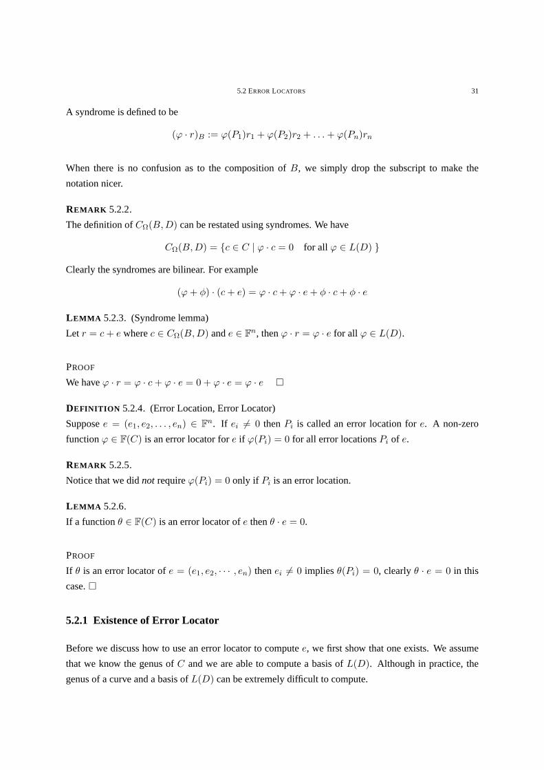
Let ϕi = xi and lethi,j = ϕiϕj · e. By Corollary5.3.3 we need to compute the following to obtain an

5.4 EXAMPLES OF SV DECODING 37

error locator (h0,0 h0,1 h0,2

h1,0 h1,1 h1,2

)Herehi,j = ϕi+j · e and all the above entries are computable. Solving for

(0 3 5

3 5 4

)α1

α2

α3

=

0

0

0

We get(α1, α2, α3) = (3, 3, 1). Soφ = 3 + 3x + x2 is error locator. We see thatφ = (x − 1)(x − 3)

which implies that onlyP1 andP3 are zeroes ofφ. Therefore the errors must be confined to those two

locations. SinceL(3Q) contains an error locator and

d(CΩ(B, 2Q)) ≥ d∗(CΩ(B, 2Q)) = 4 > d(3Q)

hence by Corollary5.2.10, we can solve the following to obtain the error vector1 1

1 3

1 32

(e2

e4

)=

1 · ex · ex2 · e

=

0

3

5

We gete2 = 2 ande4 = 5 which gives us the error vector ase = (0, 2, 0, 5, 0, 0, 0) as given.

EXAMPLE 5.4.2. (Hermitian Curve)

Consider the2-Hermitian Curve form 2. Recall that the codeCΩ(B, 5Q) hasd∗ = 5, andF4 = F2[w]

wherew2 +w +1 = 0, see Example 4.4.2. We use the following codewordc, error worde and recieved

word r

c = (1, 1, 1, 1, 1, 1, 1, 1)

e = (0, 0, w, 0, 0, 0, 0, 0)

r = (1, 1, w2, 1, 1, 1, 1, 1)

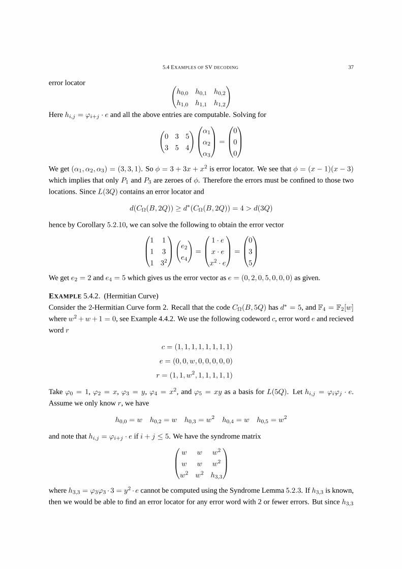
Takeϕ0 = 1, ϕ2 = x, ϕ3 = y, ϕ4 = x2, andϕ5 = xy as a basis forL(5Q). Let hi,j = ϕiϕj · e.

Assume we only knowr, we have

h0,0 = w h0,2 = w h0,3 = w2 h0,4 = w h0,5 = w2

and note thathi,j = ϕi+j · e if i + j ≤ 5. We have the syndrome matrix w w w2

w w w2

w2 w2 h3,3

whereh3,3 = ϕ3ϕ3 · 3 = y2 · e cannot be computed using the Syndrome Lemma5.2.3. If h3,3 is known,

then we would be able to find an error locator for any error word with 2 or fewer errors. But sinceh3,3

5.4 EXAMPLES OF SV DECODING 38

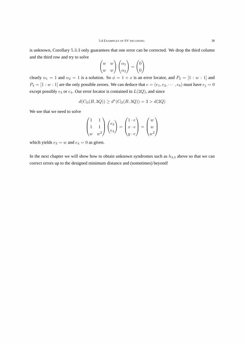
is unknown, Corollary5.3.3 only guarantees that one error can be corrected. We drop the third column

and the third row and try to solve (w w

w w

)(α1

α2

)=

(0

0

)clearlyα1 = 1 andα2 = 1 is a solution. Soφ = 1 + x is an error locator, andP3 = [1 : w : 1] and

P4 = [1 : w : 1] are the only possible zeroes. We can deduce thate = (e1, e2, · · · , e8) must haveej = 0

except possiblye3 or e4. Our error locator is contained inL(2Q), and since

d(CΩ(B, 3Q)) ≥ d∗(CΩ(B, 3Q)) = 3 > d(2Q)

We see that we need to solve1 1

1 1

w w2

(e3

e4

)=

1 · ex · ey · e

=

w

w

w2

which yieldse3 = w ande4 = 0 as given.

In the next chapter we will show how to obtain unknown syndromes such ash3,3 above so that we can

correct errors up to the designed minimum distance and (sometimes) beyond!

CHAPTER 6

Majority Voting Algorithm

6.1 Introduction

From the last chapter we saw that the SV-Algorithm can only correct up tot∗ − g/2 errors, where

theoretically at leastt∗ errors are correctable. The breakthrough can be found in([2], 93) where Feng

and Rao utilized a Majority Voting Scheme (MVS) to obtain the unknown syndromes for a One-Point

codes via a "voting process". During the revision phase of the paper Duursma derived a generalization

of Feng-Rao’s MVS to arbitrary divisors. In this chapter, we will treat the One-Point codes first and

define the Feng-Rao minimum distance which is better than designed minimum distance in many cases.

From there we present Duursma’s extension.

Assumptions

Throughout, letC be a non-singular projective curve. LetB :=∑n

i=1 Pi wherePi ∈ C are distinct

rational points. We also letD be an arbitrary divisor withsupp(D) ∩ supp(B) = ∅.

6.2 Majority Voting Scheme for One-Point Codes

We will consider One-Point codes and the decoding algorithm (MVS) that allows us to decode upto

half the designed minimum distance and sometimes beyond! In the last chapter, the difficulty we had

was that not all the syndromes can be computed. So our main aim is to compute the syndromes by other

means. We start by developing some theory of Weierstrass points, crucial to the theoretical underpinning

of the MVS.

Throughout, letD = mQ wherem = 2g + 2t∗ − 1, therefored∗(CΩ(B,D)) = 2t∗ + 1 implying that

at leastt∗ errors may be corrected.

39

6.2 MAJORITY VOTING SCHEME FORONE-POINT CODES 40

6.2.1 Basic Weierstrass Points theory

Let P ∈ C be a rational point. We would like to study the values ofm wherel(mP ) = l((m − 1)P ).

These values are related to an improved estimate of the minimum distance named after Feng and Rao

proposed in([3], 95). We will derived these results using the Riemann-Roch theorem.

DEFINITION 6.2.1. (Gap, Non-Gap)

Let P ∈ C. For anym ∈ N, if l(mP ) = l((m−1)P ) thenm is called a gap. Otherwisem is a non-gap.

We denote the set of gaps ofP by G(P ).

L EMMA 6.2.2.

The setN \G(P ) for anyP ∈ C is a semigroup with respect to addition.

PROOF

Supposem,n ∈ N \ G(P ), then there existsϕ ∈ L(mP ) andφ ∈ L(nP ) whereordP (ϕ) = m and

ordP (φ) = n. The productϕφ ∈ L((m+n)P ) but does not lie inL((m+n−1)P ), som+n ∈ N\G(P ).

The associativity of the non-gaps is clear.

L EMMA 6.2.3.

The gapsG(P ), is a subset of1, 2, · · · , 2g − 1. Moreover there are exactlyg gaps.

PROOF

Clearly, l(−kP ) = 0 for k positive. So0 /∈ G(P ). Now we establish thatn ∈ G(P ) impliesn ≤ 2g

via a proof by contradiction. Supposen > 2g (son− 1 > 2g − 1), by Riemman-Roch we have

l(nP ) = n + 1− g 6= n− g = l((n− 1)P )

therefore we haveG(P ) ⊆ 1, 2, · · · , 2g − 1. Also by Riemann Roch we have

l((2g − 1)P ) = 2g − 1 + 1− g = g

which helps us to derive the following inequilities

1 = l(0P ) ≤ l(P ) ≤ l(2P ) ≤ · · · ≤ l((2g − 1)P ) = g

Together with the fact that0 ≤ l(D + P ) − l(D) ≤ 1 for any divisorD, we see that there must be

exactlyg − 1 values ofm for which l((m − 1)P ) + 1 = l(mP ) for m between 1 and2g − 1. Hence

there are(2g − 1)− (g − 1) = g gaps.

REMARK 6.2.4.

A Weierstrass Point is a point whereG(P ) 6= 1, 2, · · · , g. There are only a finite number of Weier-

strass points on any curve.

6.2 MAJORITY VOTING SCHEME FORONE-POINT CODES 41

6.2.2 Preliminaries

DEFINITION 6.2.5.

A One-Point code is a residue codeCΩ(B,D) whereD = sP for somes ∈ N andP ∈ C.

Let Xi for i ∈ N be a sequence of divisors such thatl(Xi) = i andXi = jP for somej ∈ N \ G(P ).

As an immediate consequence we see thatXi ≤ Xi+1 for all i, D = Xt∗+2g , andordP (ϕi) = −d(Xi).

Throughout we assume that

L(Xi) = 〈ϕj | j = 1, 2, · · · , i〉

As in the last chapter, an error locator exists inL(Xt∗+1) and we see that

l(Xt∗+g) = t∗ + g = d(Xt∗+g) + 1− g; by Riemann-Roch

⇒ d(Xt∗+g) = t∗ + 2g − 1

⇒ d∗(CΩ(B,Xt+g)) = t∗ + 1

We know thatXt∗+g can be used in conjunction withXt∗+1 to find any error worde of weight less than

or equal tot∗, provided we can compute the following matrix of syndromes

S :=

ϕ1ϕ1 · e ϕ1ϕ2 · e · · · ϕ1ϕt+1 · eϕ2ϕ1 · e ϕ2ϕ2 · e · · · ϕ2ϕt+1 · e

......

......

ϕt∗+gϕ1 · e ϕt∗+gϕ2 · e · · · ϕt∗+gϕt∗+1 · e

But we will see that it is more beneficial to consider a largers×s matrix wheres = max(t∗+1, t∗+g).

Therefore, from here on we will consider

S :=

ϕ1ϕ1 · e ϕ1ϕ2 · e · · · ϕ1ϕs · eϕ2ϕ1 · e ϕ2ϕ2 · e · · · ϕ2ϕs · e

......

......

ϕsϕ1 · e ϕsϕ2 · e · · · ϕsϕs · e

; s = max(t∗ + 1, t∗ + g)

REMARK 6.2.6.

In many texts,S is assumed to be a(t∗ + g) × (t∗ + g) syndrome matrix instead. This is a minor

oversight, since ifg = 0 then we should consider the(t∗ + 1)× (t∗ + 1) syndrome matrix to ensure that

an error locator can be found.

REMARK 6.2.7.

By the theory we have developed in the last chapter, we see thatXt∗+g can be replaced byXt+k,

providedk satisfiiesd(CΩ(B,Xt+k)) ≥ t + 1 andt = b d−12 c for some the minimum distance estimate

d.

6.2 MAJORITY VOTING SCHEME FORONE-POINT CODES 42

Notation

SupposeM be a matrix. ThenM≤u,≤v denotes the submatrix ofM consisting of the intersection of the

first u rows andv columns.

For convenience we defineΦ(i, j) := d(Xi) + d(Xj), anddij := l(Φ(i, j)P )

6.2.3 Rank Matrices, Pivots and Non-Pivots

In this section, we aim to discuss the main insights of the Majority Voting Scheme informally in order

to build an intuition about why the method works. In particular, we will introduce an original novel

approach via rank matrices.

DEFINITION 6.2.8. (Rank Matrix)

Let M be a matrix with entries coming fromF. DefineRM , the rank matrix ofM to be the matrix where

the (i, j)th entry is the rank of the submatrixM≤i,≤j . We adopt the convention thatRM = (ri,j) and

definer0,i = 0 = ri,0 for all i andj. Note thatRM has the same shape asM , and ther0,j ’s andri,0’s

are not entries ofRM .

REMARK 6.2.9.

We will see that the rank matrix helps us to visualise the majority voting scheme, providing an interesting

insight into the problem.

DEFINITION 6.2.10. (Totally Rank Equivalent)

We callM andM ′ totally rank equivalent (TRE) ifRM = RM ′ , and we writeM ≡R M ′.

REMARK 6.2.11.

The relation≡R, is indeed an equivalence relation. More interesting however, is thatRM ≡R M . As a

consequence, the theory of rank matrices allows us to study a large class of matrices simultaneously.

L EMMA 6.2.12.

Let RM be the rank matrix ofM and letRM = (ri,j). We have

a) ri,j ≤ ri+1,j ≤ ri,j + 1

b) ri,j ≤ ri,j+1 ≤ ri,j + 1

c) ri,j ≤ ri+1,j+1 ≤ ri,j + 2

PROOF

Consider the submatricesM≤i,≤j and M≤i+1,≤j . The latter is the former with an added row. The

(i + 1)th row of M≤i+1,≤j is either a linear combination of the other rows, in which caseri,j = ri+1,j

by definition, or it is linearly independent of the other rows and we haveri,j + 1 = ri+1,j . For part b)

considerMT≤i,≤j andMT

≤i,≤j+1 and apply a). For c), apply a) and then b).

6.2 MAJORITY VOTING SCHEME FORONE-POINT CODES 43

Consider am×n matrixM of rankr. By Lemma6.2.12, theri,j ’s increase at most by one for successive

values ofi andj, and additionallyrm,n = r. Hence we can conclude that there are at most2r positions

of i, j whereri,j < ri+1,j or ri,j < ri,j+1. Assume without loss of generality thatr ≤ m ≤ n. The ratio

of the entries that are larger than entries on the previous row of column is at most2rmn ≤

2mmn = 2

n . For

n large, this ratio is small. This insight motivates the following definition.

DEFINITION 6.2.13. (Pivot, Non-Pivot)

Let M be a matrix with rank matrixRM = (ri,j), and recallr0,j = 0 = ri,0 for all i andj. A pivot of

M is a position(i, j) where

ri,j 6= ri−1,j−1 = ri−1,j = ri,j−1

If (i, j) is not a pivot then it is called a non-pivot.

L EMMA 6.2.14.

Let M be a matrix,r be the rank ofM andRM = (ri,j), then

a) If (i, j) is a pivot then(i′, j)and(i, j′) are non-pivots for alli′ > i andj′ > j

b) The number of pivots ofM is equal to the rank ofM

PROOF

Suppose(i, j) is a pivot so we haveri,j−1 + 1 = ri,j . Now ri+1,j cannot be a pivot sinceri,j−1 6= ri,j .

If ri+1,j−1 = ri+1,j−1 + 1 thenri+1,j = ri+1,j + 1 since if the first(i + 1)th row restricted to the

j−1 columns is linearly indepedent of the previous row then adding another column will not change the

linear independence. In this way we see that(i + 2, j) can not be a pivot either sinceri+1,j 6= ri+1,j−1.

Continuing in this way, we see that(i′, j) can not be pivots for alli′ > i if (i, j) is. An identical argument

can be applied to show that(i, j′) are not pivots for allj′ > j.

If (i, j) is a pivot thenri,j > ri−1,j−1, but r ≥ ri,j , so the number of pivots is less thanr. But by

part a) the pivots are on different rows, and each row that contains a pivot is linearly independent of the

previous rows. So the number of pivots must equal to the number of linearly independent rows, which

is the rank.

6.2.4 Application to Decoding

Recall that we definedS = (si,j) wheresi,j := ϕiϕj · e. Also, recall that we need to be able to compute

all the values ofS to ensure that an error locator can be found for all error vectore with wt(e) ≤ t∗.

Unfortunately, ifd(Xi) + d(Xj) > 2t∗ + 2g − 1, then there is no easy way of computingsi,j .

By the discussion in the previous section, the ratio of pivots to non-pivots ofS is at most1/ max n, m

for am× n matrixS. Supposesi,j is unknown, then we should "guess" that it is a non-pivot, since that

is more likely.

6.2 MAJORITY VOTING SCHEME FORONE-POINT CODES 44

It turns out that if(i, j) is a non-pivot satisfying the following relations

ri,j = ri−1,j−1 = ri−1,j = ri,j−1

then we can produce a guess value forsi,j . There is no known way of producing a good guess value for

si,j if (i, j) does not satisfy the above. This motivates the following definition and theorem.

DEFINITION 6.2.15. (Good non-pivot, Bad non-pivots)

A non-pivot(i, j) is good if

ri,j = ri−1,j−1 = ri−1,j = ri,j−1

Other non-pivots are referred to as bad.

THEOREM 6.2.16.

Let S be a matrix overF. Letsk denote thekth row ofSi,j−1 and letRS = (ri,j). Suppose(i, j) satisfies

ri−1,j−1 = ri−1,j = ri,j−1

then it is either a good non-pivot or a pivot, and

si =i−1∑k=1

αksk (6.1)

for someαi ∈ F. Furthermore, ifsi,j is a good non-pivot then

si,j =i−1∑k=1

αksk,j

PROOF

Clearly, (i, j) is either a pivot or a good non-pivot by definitions6.2.13 and6.2.15. Since we have

ri−1,j−1 = ri,j−1, this tells us that there exists a linear row relation inSi,j−1, such that theith row of

Si,j−1 is expressible as a linear combination of the other rows. Suppose we have a linear relation as in

(6.1). Apply the following row operations

ri ← ri −i−1∑k=1

αkrk

to Si,j to obtainS′i,j . We have

S′i,j =

s1,1 s1,2 · · · · · · s1,j

s2,1 s2,2 · · · · · · s2,j

......

......

...

0 0 · · · 0 x

6.2 MAJORITY VOTING SCHEME FORONE-POINT CODES 45

where the valuex must satisfy the following (by the row operations we applied),

x = si,j −i−1∑k=1

αksk,j (6.2)

We also haveri−1,j = ri−1,j−1, i.e. thejth column ofSi−1,j is expressible as a linear combination of

the other columns, therefore we can apply column operations of the form

cj ← cj −j−1∑k=1

βkck

to S′i,j and obtainS′′i,j such that

S′′i,j =

s1,1 s1,2 · · · · · · 0

s2,1 s2,2 · · · · · · 0...

......

......

......

...... 0

0 0 · · · 0 x

We note that theith row of S′′i,j is the same asS′i,j since the column operations had the effect of only

adding zeroes tox. Note also that the row and column operations applied toSi,j andS′i,j do not affect

the submatrixSi−1,j−1. Furthermore, applying row and column operations do not affect the rank.

Now if (i, j) is a pivot thenx 6= 0 since in that caseri,j > ri−1,j−1. On the other hand, if(i, j) is a

good non-pivot thenx = 0 since we requireri,j = ri−1,j−1.

By (6.2), we have

si,j =j−1∑k=1

αksi,k

as required.

Based on the above theorem, we have a way of making an educated "guess" for the value ofsi,j when

(i, j) satisfiesri−1,j−1 = ri−1,j = ri,j−1, by assuming that(i, j) is a good non-pivot. Note that if(i, j)

is a pivot then it also satisfiesri−1,j−1 = ri−1,j = ri,j−1. In fact if si,j is unknown then there is no

straightforward way of determining whether(i, j) is a pivot or a good non-pivot. We summarise the

discussion in the following corollary.

COROLLARY 6.2.17.

Supposesi,j satisfies

ri−1,j−1 = ri−1,j = ri,j−1

6.2 MAJORITY VOTING SCHEME FORONE-POINT CODES 46

and

si =i−1∑k=1

αksk

wheresk is thekth row ofSi,j−1 andαk ∈ F for all k, then

si,j =i−1∑k=1

αksk,j

if and only if (i, j) is a good non-pivot.

PROOF

As in the proof of theorem, if(i, j) is good pivot thensi,j =∑i−1

k=1 αksk,j . On the other hand, if(i, j)

is a pivot then the value ofx must be non zero, and

si,j =i−1∑k=1

αksk,j + x

instead.

REMARK 6.2.18.

The corollary tells us that any row relation involvingsi allows us to uniquely determine the value ofsi,j ,

if (i, j) is a good non-pivot. The theorem makes use of all the properties of a good non-pivot, and there

is no obvious extension to guessing the value ofsi,j if it is a bad non-pivot. Also, if we produce a guess

value forsi,j assuming that it’s a good non-pivot, then our guess will be wrong if it is indeed a pivot.

L EMMA 6.2.19.

Let M be a matrix and letri,j be the(i, j)th entry ofRM . The position(i, j) is a bad non-pivot if and

only if there exists(i′, j) or (i, j′) such that(i′, j) or (i, j′) is a pivot for somei′ < i or j′ < j.

PROOF

Suppose(i′, j) is a pivot for somei′ < i. By Lemma6.2.14, (i, j) must be a non-pivot. Further, by

definition of a pivot we must have(i′, j − 1) < (i′, j), so(i, j − 1) < (i, j) and therefore it cannot be a

good non-pivot. The case(i, j′) being a pivot for somej′ < j is entirely analogous.

6.2 MAJORITY VOTING SCHEME FORONE-POINT CODES 47

Conversely, suppose(i, j) is bad non-pivot then we can classify them into one of the four different types

listed below

Type 1

(ri−1,j−1 ri−1,j

ri,j−1 ri,j

)=

(k − 1 k

k k

)

Type 2

(ri−1,j−1 ri−1,j

ri,j−1 ri,j

)=

(k − 2 k − 1

k − 1 k

)

Type 3

(ri−1,j−1 ri−1,j

ri,j−1 ri,j

)=

(k − 1 k

k − 1 k

)

Type 4

(ri−1,j−1 ri−1,j

ri,j−1 ri,j

)=

(k − 1 k − 1

k k

)

For type 1, we must haveri−2,j−1 = k − 1 or k − 2 since the rank values on the same column and

successive rows must only differ by at most one by Lemma6.2.12. If ri−2,j−1 = k − 1, then by

applying Lemma6.2.12 again, either (1)ri−1,j = k in which caseri−2,j−1 ri−2,j

ri−1,j−1 ri−1,j

ri,j−1 ri,j

=

k − 1 k

k − 1 k

k k

which reduces to type 3; or (2)ri−1,j = k yieldingri−2,j−1 ri−2,j

ri−1,j−1 ri−1,j

ri,j−1 ri,j

=

k − 1 k − 1

k − 1 k

k k

in which case we can easily see that(i− 1, j) is a pivot.

If ri−2,j−1 = k − 2 thenri−2,j must equalk − 1, because the only other alternativeri−2,j = k violates

Lemma6.2.12; so we have ri−2,j−1 ri−2,j

ri−1,j−1 ri−1,j

ri,j−1 ri,j

=

k − 2 k − 1

k − 1 k

k k

Clearly this reduces to type 2.

Now to type 2, again, eitherri−2,j−1 = k − 1 and (1)ri−2,j = k − 1 or (2) ri−2,j = k − 2 ; or (3)

ri−2,j−1 = k − 2 andri−2,j = k − 1. Following a similar argument set out in proving type 1, we see

that case (1) reduces to type 3, case (2) gives that(i− 1, j) is a pivot, and case (3) gives

6.2 MAJORITY VOTING SCHEME FORONE-POINT CODES 48ri−2,j−1 ri−2,j

ri−1,j−1 ri−1,j

ri,j−1 ri,j

=

k − 3 k − 2

k − 2 k − 1

k − 1 k

which reduces back to type 2. But we see that a type 2 sometimes can not be reduced back to a type

2 sinceri,j ≥ 0 by definition, so if we apply our analysis to the type 2 problem above, we see that

eventually it must reduce to case (1) or (2). This proves type 2.

It remains to show that type 3 satisfies the theorem and note that type 4 can be solved by considering its

transpose as type 3. Again we have 3 cases: (1)ri−2,j−1 = k−1 andri−2,j = k or (2)ri−2,j−1 = k−1

andri−2,j = k − 1 ; or (3) ri−2,j−1 = k − 2 andri−2,j = k − 1. Case (1) reduces to type 3, but this

reduction can not always happen sincer0, j − 1 = 0 by definition, so as we traversei, i− 1, · · · , 0, we

see thatri−a,j−1 > rr−a+1,j−1 or ri−a,j > rr−a+1,j for somea ∈ N which in effect reduces case (1)

to (2) or (3). Case (2) shows thatri−1,j is a pivot. Case (3) reduces back to type 2, but note that this

reduction is accompanied by a reduction in the value of the rank. A type 2 is sometimes reduced back

to type 3, but since the reduction from type 3 to type 2 lowers the rank value, this reduction pattern can

not continue forever, so case (3) either gets resolved by the prove for type ! 2 or it is reduced to case (1)

or (2).

To gain some more insight into the intuition behind the MVS we prove the following lemma.

L EMMA 6.2.20.

Let r be the rank ofS thenr ≤ wt(e).

PROOF

Recall,s = max (t∗ + g, t∗ + 1). We expressS as the following product of matrices

S :=

ϕ1(P1) ϕ1(P2) · · · ϕ1(Pn)

ϕ2(P1) ϕ2(P2) · · · ϕ2(Pn)...

......

...

ϕs(P1) ϕs(P2) · · · ϕs(Pn)

e1 0 · · · 0

0 e2 · · · 0...

......

...

0 0 · · · en

ϕ1(P1) ϕ2(P1) · · · ϕs(P1)

ϕ1(P2) ϕ2(P2) · · · ϕs(P2)...

......

...

ϕ1(Pn) ϕ2(Pn) · · · ϕs(Pn)

where we assumee = (e1, e2, · · · , en). Clearly, the rank ofS is at most equal to the rank of the middle

diagonal matrix, which iswt(e).

We have been arguing the case that we can produce a guess for somesi,j by assuming(i, j) is a good non-

pivot and our guesses are more likely to be correct. The next lemma shows that a lot of our seemingly

different guesses are actually guesses about the same thing. Therefore, if the majority of them are correct

then we can discover the unknown values ofsi,j via a voting process!

Recall thatΦ(i, j) := d(Xi) + d(Xj) anddij := l(Φ(i, j)P ) wherel(Xi) = i.

6.2 MAJORITY VOTING SCHEME FORONE-POINT CODES 49

L EMMA 6.2.21.

Suppose thesi,j ’s are known for all(i, j) such thatΦ(i, j) < s, for somes ∈ N, then knowing any one

si,j with Φ(i, j) = s determines all othersk,l’s with Φ(k, l) = s.

PROOF

Suppose we know the value ofsi,j with Φ(i, j) = s, then we have

si,j = α1ϕ1 · e + α2ϕ2 · e + · · ·+ αdijϕdi,j · e

If Φ(i′, j′) = s, then similarly we have

si′,j′ = α1ϕ1 · e + α2ϕ2 · e + · · ·+ αdi′j′ϕdi′,j′ · e

By assumption, we know the value ofsi,j , andϕk’s are known fork < Φ(i, j). So fromsi,j we can

derive the value forϕdi,j= ϕs = ϕdi′,j′ , which in turn determinessi′,j′ .

6.2.5 Majority Voting

In this section we will prove a number of technical results that confirm our intuition and show how we

can make use of those results to design a reasonably fast decoding algorithm we call MVS. We begin

with a definition.

Definition (Candidate, Non-candiate)

Let S = (si,j) be as before and letRM = (ri,j). Supposesu,v is an unknown syndrome but allsi,j for

i ≤ u andj ≤ v, except(i, j) = (u, v), are known. We callsi,j a candidate if(i, j) is either a good

non-pivot or pivot. Otherwise,si,j is called a non-candidate. If(i, j) is a good non-pivot, then it is a

correct or true candidate, otherwise it is called incorrect or false.

REMARK 6.2.22.

Consistent with previous discussions, a candidate is one for which we can produce a guess value for,

and our guess will be false if the position of the candidate is actually a pivot, hence the above definition.

We can now describe the MVS that completely determines the syndrome matrixS defined earlier. Firstly,

we give a description of the MVS algorithm.

Recall thatΦ(i, j) := d(Xi) + d(Xj) anddi,j := l(Φ(i, j)P ), and

L(Xi) = 〈ϕ1, ϕ2, · · · , ϕi〉

and suppose that

si,j =di,j∑k=1

βi,kϕk · e

where the values of the scalarsβi,k’s are known.

6.2 MAJORITY VOTING SCHEME FORONE-POINT CODES 50

Assume the code we use isCΩ(B,Xs) for somes ∈ N \G(P ).

The Basic MVS Algorithm

Initialised← d(Xs+1).

(1): Locate all candidates,si,j with Φ(i, j) = d. For each candidatesi,j , find a linear row relation in the

form of

si =i−1∑k=1

αi,ksk

wheresl is thelth row ofSi,j−1 andαi,k’s are scalars.

Let s′i,j ←∑i−1

k=1 αi,ksk,j , then let

gi,j =1

αi,di,j

(s′i,j −di,j−1∑k=1

αi,ksk,j)

Once all the possiblegi,j ’s are computed, letg be the value that most of thegi,j ’s take. Let

si,j ←di,j−1∑k=1

βi,kϕk · e + g

If a row/column relation is found inS then we can use that relation to compute an error-locator, and

hence the error word, and so we halt the algorithm in that case. Otherwise, if not all thesi,j are known

then incrementd by 1 and go back to step (1).

EXAMPLE 1

Consider the2-Hermitian Curve, see Example4.4.2. For Q = [0 : 1 : 0] We haveL(5Q) =

〈1, x, y, x2, xy〉, whereF4 := F2[w] andw2 + w + 1 = 0. Let

P1 = [0 : 0 : 1] P2 = [0 : 1 : 1] P3 = [1 : w : 1] P4 = [1 : w2 : 1]

P5 = [w : w : 1] P6 = [w : w2 : 1] P7 = [w2 : w : 1] P8 = [w2 : w2 : 1]

The codeCΩ(B, 5Q) can correct 2 errors and it has parity check matrix.

1 1 1 1 1 1 1 1

0 0 1 1 w w w2 w2

0 1 w w2 w w2 w w2

0 0 1 1 w2 w2 w w

0 0 w w2 w2 1 1 w

For this example we let

e = (1, 0, w, 0, 0, 0, 0)

6.2 MAJORITY VOTING SCHEME FORONE-POINT CODES 51

andφ0 = 1, φ2 = x, φ3 = y, φ4 = x2, φ5 = xy. Since the genus is 1, we need to compute the3 × 3

matrix

S =

φ0φ0 · e φ0φ2 · e φ0φ3 · eφ2φ0 · e φ2φ2 · e φ2φ3 · eφ3φ0 · e φ3φ2 · e φ3φ3 · e

=

1 · e x · e y · ex · e x2 · e xy · ey · e xy · e y2 · e

=

w2 w w2

w w 0

w2 0 y2 · e

and

RS =

1 1 1

1 2 2

1 2 r3,3

clearly(3, 3) is a candidate. The third row ofS3,2 can be expressed as the sum ofw2r1 + w2r2 where

r1 andr2 are the first and second row ofS3,2, so we guessS3,3 to bew2w2 + w20 = w4 = w. It can be

confirmed thaty2 · e = w.

REMARK 6.2.23.

For larger scale examples, see([3], 95) or Appendix B.

6.2.6 Feng-Rao Minimum Distance

We now prove a theorem that validates the MVS, where the main skeleton of the proof was sketched in

([3], 95). We start with some definitions.

DEFINITION 6.2.24.

Definedi := d(Xi). We let the set of pairsNr be defined by

Nr = (di, dj) ∈ N2 | di + dj = dr+1)

wherel(Xi) = i anddi ∈ N \G(P ).

DEFINITION 6.2.25. (Feng-Rao Minimum Distance)

Let nr denote the cardinality ofNr. The Feng-Rao minimum distancedFR of the One-Point code

CΩ(B,Xs) is defined to be

dFR = minnr | r ≥ s

L EMMA 6.2.26.

For a codeCΩ(B,Xs). We havedFR ≥ d∗, and they are equal ifd(Xs) ≥ 4g − 2, whereg is the genus

of C.

PROOF

Considernr for somer ≥ s. If d(Xs) ≤ 2g − 2, thend∗ = d(Xs)− (2g − 2) ≤ 0 which is clearly less

6.2 MAJORITY VOTING SCHEME FORONE-POINT CODES 52

thannr. So assumed(Xs) ≥ 2g − 1. Let di := d(Xi) and define the setsN , I andJ by

N := (i, dr+1 − i) | i = 0, 1, · · · , dr+1

I := (i, dr+1 − i) ∈ N | i ∈ N \G(P )

J := (dr+1 − j, j) ∈ N | j ∈ N \G(P )

then we haveNr = I ∩ J , and by the Inclusion-Exclusion Principle

|I ∩ J | = |I|+ |J | − |I ∪ J | (6.3)

For the values between0, 1, 2, · · · , dr+1 there areg non-gaps from0, 1, · · · , 2g−1 sincel((2g−1)P ) =

g for any rational pointP ∈ C. Thedr+1 − 2g + 1 values between2g anddr+1 are all non-gaps, so

|I| = g + dr+1− 2g +1 = dr+1− g +1. Note that|J | = |I| andI ∪J ⊆ N and so|I ∪J | ≤ dr+1 +1.

Substitute into (6.3), we get

nr = |I ∩ J | = dr+1 − g + 1 + dr+1 − g + 1− |I ∪ J |

≥ 2dr+1 − 2g + 2− (dr+1 + 1) (∗)

= dr+1 − 2g + 1

= dr − 2g + 2; sincedr ≥ 2g − 1 and sodr+1 = dr + 1

≥ ds − (2g − 2) =: d∗; by assumptiondr ≥ ds

ThereforedFR := minnr | r ≥ s ≥ d∗. Now if ds ≥ 4g − 2 ⇒ dr+1 ≥ 4g − 1, thenI ∪ J = N

since if i /∈ N(P ) thendr+1 − i ≥ 4g − 1 − (2g − 1) = 2g is a non-gap, so(i, j) ∈ N implies either

(i, j) ∈ I or (i, j) ∈ J . So(∗) is an equality and hencedFR := minnr | r ≥ s = ns = d∗.

THEOREM 6.2.27.

Consider the codeCΩ(B,Xs). Let di := d(Xi). Suppose thesi,j ’s are known for all(i, j)’s with

di + dj ≤ dr. Additionally, supposewt(e) ≤ (nr − 1)/2. Then the setNr has more good non-pivots

then pivots.

PROOF

This proof is based on the proof sketched in([13], 95). Let K be the number of known pivots inS, let

F be the number of pivots in the setNr, and letT the number of good non-pivots inNr. We must have

K + F less than the total number of pivots, and so

K + F ≤ rankS ≤ wt(e) (6.4)

If (i, j) is a pivot then(i′, j) and(i, j′) for i′ > i andj′ > j are all bad non-pivots, so the setNr consists

of at most2K bad non-pivots. Note that any element(di, dj) ∈ Nr fit into three categories:(i, j) is a

6.2 MAJORITY VOTING SCHEME FORONE-POINT CODES 53

pivot, a good non-pivot, or a bad non-pivot. Therefore

nr ≤ T + F + 2K

which implies

wt(e) ≤ (nr − 1)/2 ≤ (T + F )/2 + K − 1/2

Combine with(6.4) yieldsF < T as required.

COROLLARY 6.2.28.

For a codeCΩ(B,Xs), the MVS can correct all error worde satisfying

wt(e) ≤ (dFR − 1)2

PROOF

Initially, all the sydnromessi,j for di,j ≤ ds are known. By the theorem, the syndromessi,j with

di + dj = ds+1 can be obtained via the MVS since(nr − 1)/2 ≥ (dFR − 1)/2 ≥ wt(e). Now we

can obtain the syndromes that satisfydi + dj = ds+2. Clearly this process may be repeated until all the

required syndromes are obtained.

REMARK 6.2.29.

It may be noted that not all the syndromes that we claim to be computable are situated in the matrix

S which is a(t∗ + g) × (t∗ + g) matrix if g ≥ 1. For example,sk,t∗+g+1 is not an element ofS for

anyk. But if sk,t∗+g+1 is a candidate, thensk,t∗+g+1 must have been a good non-pivot. Which means

that thekth row ofS≤k,≤t∗+g is expressible as a linear row relation of the previous rows, in which case

the MVS would have halted. So if the algorithm needs to computesk,t∗+g+1, thensk,t∗+g+1 must be a

non-candidate. Hence it does not contribute a vote, and so it can be ignored.

REMARK 6.2.30.

We see thatdFR is a better measure of the minimum distance thand∗. Therefore we can consider a

smaller syndrome matrixS of shapes′ × s′ wheres′ = max(t + g, t + 1) andt = (dFR − 1)/2.

The following example demonstrates the superiority of the Feng-Rao minimum distance to the designed

minimum distance. We consider the codeCΩ(B,D) whereC is the4-Hermitian codes form 2. Recall

thatordQ(x) = −4 andordQ(y) = −5 for Q = [0 : 1 : 0]. The non-gaps are

0, 4, 5, 8, 9, 10, 12, 13, 14, 15, · · ·

6.3 THE GENERAL ALGORITHM 54

Let dr := d(Xr), whereXr = drP andL(Xr) = r. Recall thatg = 6 and so4g − 2 = 22 and

2g − 2 = 10. We have

dr 5 8 9 10 12 13 14 15 16

dr+1 8 9 10 12 13 14 15 16 17

nr 3 4 3 4 6 6 4 5 8

dFR 3 3 3 4 4 4 4 5 8

d∗ − − − 0 2 3 4 5 6

17 18 19 20 21 22

18 19 20 21 22 23

9 8 9 10 12 12

8 8 9 10 12 12

7 8 9 10 11 12

The− symbol denotes a minimum distance that cannot be estimated withd∗. Clearly,dFR is superior to

d∗ in many cases. The difference is very pronounced in a class of codes defined over the Suzuki curves.

See Example 8.4([3], 95).

6.3 The General Algorithm

6.3.1 Definitions and Preliminaries

The general MVS is very similar to the One-Point code MVS. Throughout, assume we are considering

a codeCΩ(B,D), and by a curve we mean a non-singular projective curve.

DEFINITION 6.3.1. (µ-Order)

Let C a curve, letP ∈ C and letX be a divisor. Define

µX,P (φ) := minm | φ ∈ L(X − d(X)P + mP ); if defined

:= ∞; otherwise

REMARK 6.3.2.

Theµ-order provides an indexing of functions similar to that of the indexing via order atP in the MVS

for One-Point codes. Note that ifX = dsP for someds ∈ N \G(P ) thenµX,P (ϕi) = −ordP (ϕi).

DEFINITION 6.3.3. (Gaps, Non-Gaps)

Let C be a curve. LetX be a divisor and letP ∈ C. Define the gaps ofX atP by

GX(P ) := m | l(X − d(X) + mP ) = l(X − d(X) + (m− 1)P )

The elements ofN \ GX(P ) are called the non-gaps ofX at P . Any elementa ∈ GX(P ) is called a

X-gap, similarly any elementb ∈ N \GX(P ) is called aX-non-gap.

REMARK 6.3.4.

The above definitions are generalisations of the Weierstrass Points gaps and non-gaps. It can be seen

that if we setX = 0, then the definitions above agrees with the definitions of gaps and non-gaps in the

One-Point code case. By almost exactly the same proof as Lemma6.2.3, we see that there are exactlyg

6.3 THE GENERAL ALGORITHM 55

gaps between1 and2g−1. Indeed, clearlyd(X−d(X)P +(2g−1)P ) = 2g−1 which by the Riemann-

Roch theorem implies thatl(X − d(X)P + (2g − 1)P ) = g. Sincel(E) ≤ l(E + P ) ≤ l(E) + 1 for

any divisorE, there must beg − 1 X-gap between1 and2g − 1 from which our claim follows.

DEFINITION 6.3.5. (Duursma sequence)

The Duursma sequence ofX with respect toP is the sequence of divisorsXi wherel(Xi) = i and

Xi = X − d(X)P + mP for somem ∈ N \GX(P ).

We prove some properties of the Duursma sequence.

L EMMA 6.3.6.

Let (Xi) be the Duursma sequence of a divisorX with respect toP .

1) If φ ∈ L(Xi+1) \ L(Xi) thenµX,P (φ) = d(Xi).

2) If X = 0 then for anyφ ∈ L(Xi), we have

µX,P (φ) = −ordP (φ)

3) If d(Xi) ≤ d(X) thenXi ≤ X

PROOF

LetXi = X−d(X)P +mP andXi+1 = X−d(X)P +nP where clearlyd(Xi) = m andd(Xi+1) = n.

Let φ ∈ L(Xi+1) \ L(Xi), thenµX,P (φ) > m or elseφ ∈ L(Xi). Clearly µX,P (φ) = d(Xi) by

definition.

If X = dsP for someds ∈ N \G(P ), then

µX,P (φ) := mink | φ ∈ L(X − d(X)P + kP ) = mink | φ ∈ L(kP ) = −ordP (φ)

If d(Xi) ≤ d(X) then we must haved(Xi) = m ≤ d(X) whereXi = X − d(X)P + mP for some

m ∈ N \GX(P ). ClearX ≥ X + (m− d(X))P = Xi.

DEFINITION 6.3.7.

Let C be a curve. LetX andY be divisors, letP ∈ C, and let(Xi) and(Yi) be the Duursma sequence

of X andY , respectively, with respect toP . Additionally, let(Wi) be the Duursma sequence ofX + Y

with respect toP . Define

NPX,Y,r := (d(Xi), d(Yj)) | d(Xi) + d(Yj) = d(Wr+1)

L EMMA 6.3.8.

If µX,P (ϕ) = a <∞ andµY,P (φ) = b <∞ thenµX+Y,P (ϕφ) = a + b.

6.3 THE GENERAL ALGORITHM 56

PROOF

Clearlyϕφ ∈ L(X + Y − (d(X) + d(Y ))P + (a + b)P ) and soµX+Y,P (ϕφ) ≤ a + b. We can see that

ordP (ϕ) = d(X)−XP − a

whereXP is the coefficient ofP in the divisorX, sinceϕ ∈ L(X − d(X)P + a) wherea is minimal.

Similarly

ordP (φ) = d(Y )− YP − b

whereYP is the coefficient ofP in the divisorX. Lastly

ordP (ϕφ) = d(X + Y )− (X + Y )P − µX+Y,P (ϕφ)

The three equations above are related byordP (ϕφ) = ordP (ϕ) + ordP (φ) which gives

d(X + Y )− (X + Y )P − µX+Y,P (ϕφ) = d(X)−XP − a + ordP (φ) + d(Y )− YP − b

rearrange and we get the result required.

6.3.2 The General MVS

Given a codeCΩ(B,D), we aim to adapt the MVS algorithm developed for One-Point codes to help

decode received words. HereD is generally not assumed to be of the formdsP for someP ∈ C and

ds ∈ N.

Let L(D) = 〈ϕdi| di = d(Di)〉 whereP /∈ supp(B). Let (Di) be the Duursma sequence ofD with

respect toP . Note that Lemma6.3.6 givesDi ≤ D if d(Di) ≤ d(D) and so every function inL(D)

have aµ-order ofD with respect toP .

Let s = maxt + 1, t + g whereg is the genus ofC and t = b d−12 c whered is some estimate of

minimum distance such as the generalised minimum distance defined below. Let(Yi) be the Duursma’s

sequence for the zero divisor with respect toP . Let yi := d(Yi) and letL(Yi) = 〈φyj | j ≤ i〉, we

consider the syndrome matrix

S :=

ϕd1φy1 · e ϕd1φy2 · e · · · ϕd1φys · eϕd2φy1 · e ϕd2φy2 · e · · · ϕd2φys · e

......

......

ϕdsφy1 · e ϕdsφy2 · e · · · ϕdsφys · e

As before, if we know enough of the syndromes to find a linear row or column relation, then we can find

an error locator and hence the error.

By Lemma6.3.8, we see that

µD+0,P (ϕiφj) = µD,P (ϕiφj) = i + j

6.3 THE GENERAL ALGORITHM 57

and soi + j = i′ + j′ = k is the minimum value such that

ϕiφj , ϕi′φj′ ∈ L(D − d(D)P + kP )

therefore if we try to produce a guess for the positions(di, dj) and(di′ , dj′), then they are guesses about

the same thing. Hence the MVS we developed in the previous section can be applied with minimal

modification.

Using the definitions above we see that the theory we developed for One-Point codes is naturally ex-

tended to solving the problem for a general residue codeCΩ(B,D). Note thatl(Dt+1) = t + 1 and

l(Yt+1) = t + 1 and so error locators can be found inL(Dt+1) or L(Yt+1). So the natural extension is

to look for linear row relations inS as well as linear column relations. Note that theµ-order provided

a way to index the functions similar to that found in the One-Point code MVS, and this is important for

the definition of the generalised Feng-Rao Minimum distance given below. Also worthing noting is that

our choice of theφi’s andϕj ’s ensured that as many syndromes are computable as possible.

REMARK 6.3.9.

In the One-Point code case, we have(Di) = (Yi). Therefore the syndrome matrixS given above would

have been symmetric and hence looking for row relations is the same as looking for column relations.

DEFINITION 6.3.10. (Generalised Feng-Rao minimum distance)

Consider a codeCΩ(B,D). Let (Di) be the Duursma sequence ofD with respect toP /∈ supp(B), and

let nr := |NPD,0,r| assumingD = Dl(D). The generalised Feng-Rao minimum distance with respect to

P is defined to be

dPFR := minnr | r ≥ l(D)

REMARK 6.3.11.

The requirement thatP /∈ supp(B) ensures that the syndromessi,j = ϕiφj · e are defined for alli and

j.

The validity of the MVS in the general setting is verifiable by essentially the same proofs as in the

One-Point code case.

L EMMA 6.3.12.

For a codeCΩ(B,D), where we assumeD = Dl(D). We havedPFR ≥ d∗, and they are equal if

d(D) ≥ 4g − 2 whereg is the genus ofC andP /∈ supp(B).

PROOF

The case whered(D) ≤ 2g− 2 is clear, see Lemma6.2.26. So assumed(D) ≥ 2g− 1. Let di = d(Di)

6.3 THE GENERAL ALGORITHM 58

andyi = d(Yi) where(Di) and(Yi) are as defined above. We define the setsN , I, andJ by

N := (i, dr+1 − i) | i = 0, 1, · · · , dr+1

I := (di, dr+1 − di) ∈ N

J := (dr+1 − yj , yj) ∈ N

We haveNr = I ∩ J . There areg D-non-gaps from0 to 2g − 1. Thedr+1 − 2g + 1 values between2g

anddr+1 are allD-non-gaps, so

|I| = g + dr+1 − 2g + 1 = dr+1 − g + 1

Similarly, |J | = |I|. Note thatI ∪ J ⊆ N and so|I ∪ J | ≤ dr+1 + 1. By the Inclusion-Exclusion

Principle we get

nr = |I ∩ J | = dr+1 − g + 1 + dr+1 − g + 1− |I ∪ J |

≥ 2dr+1 − 2g + 2− (dr+1 + 1) (∗)

≥ ds − (2g − 2) =: d∗; by assumptiondr ≥ ds

The rest of the proof is entirely identical to Lemma6.2.26.

L EMMA 6.3.13.

Let Nr = NPD,0,r and letnr = |Nr|. For the codeCΩ(B,D), where we assumeD = Dl(D), anddi,

yi,(Di) and(Yi) are as defined above. Supposewt(e) ≤ (nr − 1)/2. Suppose thesdi,yj’s are known for

all (di, yj) such thatdi + dj ≤ dr. The setNr has more good non-pivots then pivots.

PROOF

This proof is very similar to Theorem6.2.27. Let K be the number of known pivots inS, let F be the

number of pivots in theNr, andT the number of good non-pivots inNr. We have as before

K + F ≤ rankS ≤ wt(e) (6.5)

Also Nr must have no more than2K bad non-pivots. Note that any element(di, yj) ∈ Nr must satisfy

one of the following:(i, j) is a pivot, a good non-pivot, or a bad non-pivot, and so

nr ≤ T + F + 2K

which with (6.5) yieldsF < T as required.

The general MVS is essentially the same as the One-Point code MVS. It proceeds by computing all

syndromes computable by the Syndrome Lemma. Then it produces guess values for all the candidates.

The syndrome table is updated using the values of the correct candidates. Continue this process until a

row or column relation is found. Recall that a column/row relation determines an error locator, and the

error locator uniquely determines the error worde.

6.3 THE GENERAL ALGORITHM 59

The correctness of the general MVS is guaranteed by the above lemma. The lemma shows that ife

satisfieswt(e) ≤ (dPFR − 1)/2, then the correct candidates outnumber the incorrect candidates at every

stage of the MVS. Hence we have solved the decoding problem for Algebraic Geometric codes!

References

[1] O. Pretzel 1992 "Error-Correcting Codes and Finite Fields" Oxford. Clarendon Press

[2] G.L. Feng T.R.N. Rao 1993. "Decoding Algebraic-Geometric Codes up to the Designed MinimumDistance" InIEEE Transactions on Information Theory, Vol39, No. 1, pages 37–45

[3] T. Hoholdt R. Pellikaan 1995. "On the decoding of algebraic-geometric codes" InIEEE Transactionson Information Theory, IT-41, pages 1589–1614

[4] O. Pretzel 1998. "Codes and Algebraic Curves" New York. Oxford University Press, Inc.

[5] W. Fulton 1969. "Algebraic Curves - An Introduction to Algebraic Geometry" pages 35–74, NewYork. W.A. Benjamin, Inc.

[6] M.F. Atiyah I.G. Macdonald 1969. "Introduction to Commutative Algebra" pages 80–84, Reading,MA. Addison-Wesley Publishing Company

[7] H. Stichtenoth 1991. "Algebraic Function Fields and Codes" pages 1–2, New York, Springe-Verlag

[8] S. Stepanov 1999. "Codes on Algebraic Curves" New York, Kluwer Academic/Plenum Publishers

[9] M. A. Tsfaman. S.G. Vladut. T. Zink 1982. "Modular curves, Shmura curves and Goppa codes beterthan the Varshamov-Gilbert bound." Math. Nachr, 109, 21-28

[10] H. Stichtenoth 1988. "A note on Hermitian codes overGF (q2)" In IEEE Trans. Inform. Theory34, pages 1345–1349.

[11] P. Morandi 1996. "Fields and Galois Theory" New York, Springer.

[12] V.S. Pless and W.C. Huffman 1998. "Handbook of Coding Theory Volume 1" Amsterdam, TheNethelands, Elsevier Science B.V.

[13] C. Kirfel and R. Pellikaan 1995. "The minimum distance of codes in an array coming fromtelescopic semigroups" InIEEE Trans. Inform. Theory, IT-41, pages 1720-1732.

[14] S.G. Vladut A.N. Skorobogatov 1990. "On the decoding of algebraic-geometric codes" InIEEETrans. Inform. Theory, 36, pages 1051-1960.

[15] I. M. Duursma 1993. "Majority coset decoding" InIEEE Trans. Inform. Theory, 39, pages1067-1070.

[16] V. D. Goppa 1981. "Codes on algebraic curves" InDokl. Akad. Nauk. SSSR, 259, pages 1289-1290.

60

APPENDIX A

Basic Coding Theory

A.1 Block Codes

DEFINITION A.1.1. (Block Code, Codeword)

Let F be a field. A block codeC, of lengthn over F is a subset ofFn. As we will only be dealing

with block codes in this essay, we will simply refer toC as just a code. Any element ofC is called a

codeword.

Throughout, assume that a block codeC is defined over a fieldF.

One of the most important parameters of a code is its minimum distance, which is defined in terms of

the Hamming distance. It measures how many errors can be corrected by the Majority Logic Decoding

(MLD) method, to be defined later.

DEFINITION A.1.2. (Weight, Hamming Distance, Minimum Distance)

Let c be a codeword. The weight ofc denotedwt(c) is defined to be the number of components ofc not

equal to zero. The Hamming distance (or just distance) betweenx, y ∈ C is d(x, y) := wt(x− y). The

distance between a codeword and a code is defined to be

d(x,C) := min d(x, c) | c ∈ C

The minimum distance of a codeC is

d(C) := mind(x, y)|x, y ∈ C

Examples:wt(0101) = 2 andd(010, 000) = 1 andd(010, 101) = 3.

L EMMA A.1.3.

The Hamming distance defined byd(x, y) := wt(x− y) is a metric.

PROOF

1) d(x, y) ≥ 0 is clear.

2) d(x, y) = wt(x − y) = wt(−(y − x)) = wt(y − x) = d(y, x); since multiplying by -1 does not

61

A.1 BLOCK CODES 62

change the weight

3) This proof follows([1], 92). Letx = (x1, x2, · · · , xn), y = (y1, y2, · · · , yn) andz = (z1, z2, · · · , zn).

Let Dx,z = i | xi 6= zi, then clearlyDx,z = S ∪ T whereS = i | xi 6= zi, xi = yi and

T = i | xi 6= zi, xi 6= yi. It follows that

|T | ≤ d(x, y)

and sincei ∈ S, thenyi = xi 6= zi. Therefore

|S| ≤ d(y, z)

which yields

d(x, z) = |Dx,z| = |S|+ |T | ≤ d(x, y) + d(y, z)

as required.

DEFINITION A.1.4. (Closest Point Set)

Let C be a code and letx ∈ C. DefinePC(x) := c ∈ C | d(x, c) = d(x,C).

REMARK A.1.5.

In this thesis,F is always finite, certainlyPC(x) must not be empty.

DEFINITION A.1.6. (Majority Logic Decoding)

The Majority Logic Decoding (MLD) scheme is the process where the received wordc + e is decoded

asPC(c + e).

The following lemma is important in that it describes when the closest point set is a singleton set. It

illustrates the importance of the minimum distance.

L EMMA A.1.7.

Let C be a code and letd(C) = 2t + 1 or d(C) = 2t + 2 for somet ∈ N. If wt(e) ≤ t, thenPC(c + e)

= c.

PROOF

Let f = c+e, then we haved(f, c) = wt(e) ≤ t. Supposec′ ∈ C andc′ 6= c such thatd(c′, f) ≤ wt(e),

then2t + 1 = d(C) ≤ d(c′, c) ≤ d(c′, f) + d(f, c) ≤ 2wt(e) ≤ 2t which is a contradiction. Therefore

c is the closest tof . The cased(C) = 2t + 2 uses exactly the same proof.

Notation

For convenience, when there is no chance of confusion we think ofPC(c + e) as an element, not a set.

REMARK A.1.8.

The above lemma says that if the receiver receivesc + e andwt(e) ≤ t, then by computingPC(c + e)

the original message can be recovered. Computing the closest point set while assumingwt(e) ≤ t is

A.2 L INEAR CODES 63

referred to as the decoding problem. A large portion of this thesis is devoted to the decoding problem

for Algebraic Geometric codes.

A.2 Linear Codes

Large block codes that lack some internal structure can be difficult to define and decode. It is even

difficult to determine whether a vector is a codeword or not. This motivates the development of linear

codes.

DEFINITION A.2.1. (Linear Code, Rank)

Let F be a field. A linear codeC, of lengthn is a three-tuple(U,G, H) whereU is a vector-subspace

of Fn andG : Fdim U → Fn is a linear operator such thatimG = U , andH : Fn → Fn−dim U such that

ker H = U . The rank ofC is the dimension ofU .

DEFINITION A.2.2. (Generator Matrix)

The linear operatorG in matrix form is called the generator matrix.

REMARK A.2.3.

Note thatG or H uniquely determinesU .

Notation

We abuse notation a little by referring to the vector spaceU as C. When there is no chance of a

confusion,C refers to the associated subspaceU . Also the linear operatorsG andH are almost always

expressed explicitly as matrices.

A code is useless if it can not convey information. So it is important to understand how we represent

information using a linear code. LetC be a linear code and letm be the rank ofC. Fix a basis of

C, say, c1, c2, ..., cm. We can represent am-digit information block,(d1, d2, ..., dm), as the vector

d1c1 + d2c2 + ... + dmcm. So every vector inC representsm-bits of information.

In coding theory, we takeF to be a finite field of sizeq, say. So a linear codeC of rank m haveqm

distinct vectors. If each vector represent a different symbol, thenC can be thought of as an alphabet of

sizeqm .

Notation

Let F = Fq. We call a linear code of lengthn, rankk and minimum distanced a q-ary [n, k, d] code.

This is standard notation.

A.2 L INEAR CODES 64

DEFINITION A.2.4. (Dual)

Let C be aq-ary [n, k, d] code. Define an inner product

〈x, y〉 :=n∑

i=1

xiyi

, wherex = (x1, x2, ..., xn) andy = (y1, y2, ..., yn). We sayx is orthogonal toy if 〈x, y〉 = 0. We

define the dual ofC to be the set

C⊥ := x ∈ Fn | 〈x, c〉 = 0 ∀ c ∈ C

REMARK A.2.5.

1. The spaceC⊥ is the orthogonal complement toC.

2. It can easily be shown thatC⊥ is a subspace ofFn and therefore is also a linear code.

3. The dimension ofC⊥ is n − k since we haveFn = C ⊕ C⊥ by an elementary result in functional

analysis.

4. We also have(C⊥)⊥ = C

DEFINITION A.2.6. (Parity Check Matrix)

Let C⊥ have basisc′1, c′2, ..., c

′n−k, and assumec′i is a row vector for alli between 1 andn− k, then the

matrix

H =

c′1

c′2...

c′n−k

is called the parity check matrix ofC.

L EMMA A.2.7.

Let H be as above, thenHcT = 0 if and only if c ∈ C.

PROOF

Clearly, if c ∈ C then〈c, c′i〉 = 0 for all i. By definition ofH, we have

HcT =

〈c′1, c〉〈c′2, c〉

...

〈c′n−m, c〉

=

0

0...

0

Conversely, supposeHcT = 0, i.e. 〈c′i, c〉 = 0 for all i between 1 andn− k. Since the inner proudct is

linear, any linear combination of thec′i’s is also orthogonal toc, i.e. every element ofC⊥ is orthogonal

to c, by definitionc ∈ (C⊥)⊥ = C.

A.2 L INEAR CODES 65

REMARK A.2.8.

Note that the parity check matrixH is the generator matrix forC⊥.

REMARK A.2.9.

The matrixH allows us to decide whether a vectorc is a codeword or not, but this does not tell us how

to computePC(c + e). Some texts do not require the rows ofH to be linearly indepedent.

L EMMA A.2.10.

Let C be a code of lengthn. Thendim C + dim C⊥ = n

PROOF

Consider the parity check matrixH as a linear operator, then we havedim imH + dim ker H = n. But

dim kerH = dim C = k and we havedim imH = rankH = dim C⊥ = n− k.

APPENDIX B

A Large Scale MVS Example

Consider the codeCΩ(B, 19Q) whereC : X5 +Y 4Z +Y Z4 = 0 is the4-Hermitian Curve form 2, and

Q = [0 : 1 : 0]. Let B = P1 + P2 + · · ·+ P16, where

P1 = [1 : w : 1]; P2 = [1 : w2 : 1]; P3 = [1 : w4 : 1]; P4 = [1 : w8 : 1];

P5 = [w3 : w : 1]; P6 = [w3 : w2 : 1]; P7 = [w3 : w4 : 1]; P8 = [w3 : w8 : 1];

P9 = [w6 : w : 1]; P10 = [w6 : w2 : 1]; P11 = [w6 : w4 : 1]; P12 = [w6 : w8 : 1];

P13 = [w9 : w : 1]; P14 = [w9 : w2 : 1]; P15 = [w9 : w4 : 1]; P16 = [w9 : w8 : 1];

We recallF[16] := F[2][w] wherew4 + w + 1 = 0. Also recall that

L(19Q) = 〈1, x, y, x2, xy, y2, x3, x2y, xy2, y3, x4, x3y, x2y2, xy3〉

By the example following Remark 6.3.24. we havedFR(CΩ(B, 19Q)) = 9. Thereforet = 4 errors can

be corrected. We consider thet + g = 10 by 10 syndrome matrixS.

Assume we know onlyc + e for somec ∈ CΩ(B, 19Q). Consider the case where

e = (0, 1, w, 0, 0, 0, 0, 0, 0, 0, 0, 0, 0, 0, 0, w, w2)

For convenience, we index the functions by their order atP , and writeϕ4i+5j = xiyj for 4i + 5j ≤ 19

noting that the representation is unique. Also, lethi,j := ϕiϕj · e and the(i, j)th position ofS refers to

66

B A L ARGE SCALE MVS EXAMPLE 67

the position thathi,j is located, instead of the position situated in theith row andjth column. We have

S :=

w8 w9 w4 w5 w3 w7 w10 w9 w11 w

w9 w5 w3 w10 w9 w11 w13 w13 w9 w6

w4 w3 w7 w9 w11 w w13 w9 w6 h5,15

w5 w10 w9 w13 w13 w9 h8,12 h8,13 h8,14 h8,15

w3 w9 w11 w13 w9 w6 h9,12 h9,13 h9,14 h9,15

w7 w11 w w9 w61 h10,10 h10,12 h10,13 h10,14 h10,15

w10 w13 w13 h12,8 h12,9 h12,10 h12,12 h12,13 h12,14 h12,15

w9 w13 w9 h13,8 h13,9 h13,10 h13,12 h13,13 h13,14 h13,15

w11 w9 w6 h14,8 h14,9 h14,10 h14,12 h14,13 h14,14 h14,15

w w6 h15,5 h15,8 h15,9 h15,10 h15,12 h15,13 h15,14 h15,15

where the values not computable by the Syndrome Lemma are shown ashi,j ’s. Let RS = (ri,j). We

compute theri,j ’s where we can and we have

RS :=

1 1 1 1 1 1 1 1 1 1

1 2 2 2 2 2 2 2 2 2

1 2 3 3 3 3 3 3 3 r5,15

1 2 3 3 3 3 r8,12 r8,13 r8,14 r8,15

1 2 3 3 4 4 r9,12 r9,13 r9,14 r9,15

1 2 3 3 4 r10,10 r10,12 r10,13 r10,14 r10,15

1 2 3 r12,8 r12,9 r12,10 r12,12 r12,13 r12,14 r12,15

1 2 3 r13,8 r13,9 r13,10 r13,12 r13,13 r13,14 r13,15

1 2 3 r14,8 r14,9 r14,10 r14,12 r14,13 r14,14 r14,15

1 2 r15,5 r15,8 r15,9 r15,10 r15,12 r15,13 r15,14 r15,15

Although we do not yet know the values ofh5,15 or h15,5, we can deduce thatr5,15 = 3 = r15,5. We

see that(8, 12), (10, 10), (12, 8) are the only candidates. Since the matrix is symmetric,(8, 12) and

(12, 8) must produce the same vote, and since there are a total of only three votes, they must be correct

candidates. We find an linear row relation inS≤8,≤10, by solving for theαi’s in the following linear

system

(α1 α2 α3

)w8 w9 w4 w5 w3 w7

w9 w5 w3 w10 w9 w11

w4 w3 w7 w9 w11 w

=(w5 w10 w9 w13 w13 w9

)

One solution is(α1, α2, α3) = (w9, w7, 0). Therefore, we have

h8,12 = w9w10 + w7w13 = w19 + w20 = w4 + w5 = w8

B A L ARGE SCALE MVS EXAMPLE 68

We haveh8,12 = x5 · e = h12,8, and recall that the values ofh5,15, h15,5 andh10,10 can be calculated

usingh8,12. Indeed,

h5,15 = h15,5 = h10,10 = y4 · e = (x5 + y) · e = h8,12 + h0,5 = w8 + w4 = w5

Updating the syndrome matrix and the rank matrix gives

S =

w8 w9 w4 w5 w3 w7 w10 w9 w11 w

w9 w5 w3 w10 w9 w11 w13 w13 w9 w6

w4 w3 w7 w9 w11 w w13 w9 w6 w5

w5 w10 w9 w13 w13 w9 w8 h8,13 h8,14 h8,15

w3 w9 w11 w13 w9 w6 h9,12 h9,13 h9,14 h9,15

w7 w11 w w9 w61 w5 h10,12 h10,13 h10,14 h10,15

w10 w13 w13 h12,8 h12,9 h12,10 h12,12 h12,13 h12,14 h12,15

w9 w13 w9 h13,8 h13,9 h13,10 h13,12 h13,13 h13,14 h13,15

w11 w9 w6 h14,8 h14,9 h14,10 h14,12 h14,13 h14,14 h14,15

w w6 w8 h15,8 h15,9 h15,10 h15,12 h15,13 h15,14 h15,15

and

RS =

1 1 1 1 1 1 1 1 1 1

1 2 2 2 2 2 2 2 2 2

1 2 3 3 3 3 3 3 3 3

1 2 3 3 3 3 3 r8,13 r8,14 r8,15

1 2 3 3 4 4 r9,12 r9,13 r9,14 r9,15

1 2 3 3 4 4 r10,12 r10,13 r10,14 r10,15

1 2 3 3 r12,9 r12,10 r12,12 r12,13 r12,14 r12,15

1 2 3 r13,8 r13,9 r13,10 r13,12 r13,13 r13,14 r13,15

1 2 3 r14,8 r14,9 r14,10 r14,12 r14,13 r14,14 r14,15

1 2 3 r15,8 r15,9 r15,10 r15,12 r15,13 r15,14 r15,15

From RS we can see that(8, 13) and(13, 8) are the candidates and so they are both true candidates,

since they produce the same vote and the number of correct votes is in the majority. Again by looking

for row relations, we get

h8,13 = w9h0,13 + w7h4,13 = w3 + w5 = w11

and

h9,12 = (xy × x3) · e = (x2 × x2y) · e = h8,13 = w11

B A L ARGE SCALE MVS EXAMPLE 69

We update the table

S =

w8 w9 w4 w5 w3 w7 w10 w9 w11 w

w9 w5 w3 w10 w9 w11 w13 w13 w9 w6

w4 w3 w7 w9 w11 w w13 w9 w6 w5

w5 w10 w9 w13 w13 w9 w8 w11 h8,14 h8,15

w3 w9 w11 w13 w9 w6 w11 h9,13 h9,14 h9,15

w7 w11 w w9 w61 w5 h10,12 h10,13 h10,14 h10,15

w10 w13 w13 w8 w11 h12,10 h12,12 h12,13 h12,14 h12,15

w9 w13 w9 w11 h13,9 h13,10 h13,12 h13,13 h13,14 h13,15

w11 w9 w6 h14,8 h14,9 h14,10 h14,12 h14,13 h14,14 h14,15

w w6 w5 h15,8 h15,9 h15,10 h15,12 h15,13 h15,14 h15,15

Continuing in this way, we get all the required syndromes

S =

w8 w9 w4 w5 w3 w7 w10 w9 w11 w

w9 w5 w3 w10 w9 w11 w13 w13 w9 w6

w4 w3 w7 w9 w11 w w13 w9 w6 w5

w5 w10 w9 w13 w13 w9 w8 w11 w2 w9

w3 w9 w11 w13 w9 w6 w11 w2 w9 h9,15

w7 w11 w w9 w61 w5 w2 w9 h10,14 h10,15

w10 w13 w13 w8 w11 w2 h12,12 h12,13 h12,14 h12,15

w9 w13 w9 w11 w2 w9 h13,12 h13,13 h13,14 h13,15

w11 w9 w6 w2 w9 h14,10 h14,12 h14,13 h14,14 h14,15

w w6 w5 w9 h15,9 h15,10 h15,12 h15,13 h15,14 h15,15

Let ci be theith column ofS. We see that

w9c1 + w7c2 + c4 = 0

From which we can deduce that

φ = w9 + w7x + x2 = (x + 1)(x + w9)

is an error locator ofe. The zeroes ofφ areP1, P2, P3, P4, P13, P14, P15 andP16. We see thatφ ∈L(8Q), and

d(CΩ(B, 19Q)) ≥ dFR(CΩ(B, 19Q)) = 9 > d(8Q)

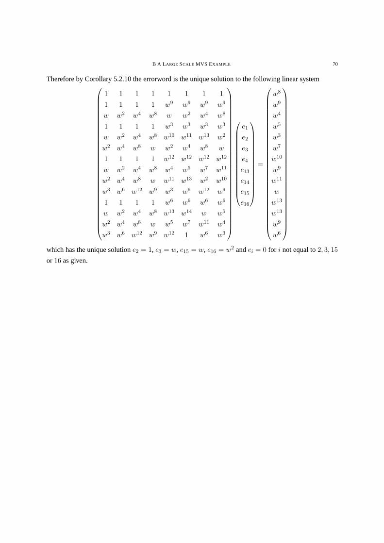
B A L ARGE SCALE MVS EXAMPLE 70

Therefore by Corollary 5.2.10 the errorword is the unique solution to the following linear system

1 1 1 1 1 1 1 1

1 1 1 1 w9 w9 w9 w9

w w2 w4 w8 w w2 w4 w8

1 1 1 1 w3 w3 w3 w3

w w2 w4 w8 w10 w11 w13 w2

w2 w4 w8 w w2 w4 w8 w

1 1 1 1 w12 w12 w12 w12

w w2 w4 w8 w4 w5 w7 w11

w2 w4 w8 w w11 w13 w2 w10

w3 w6 w12 w9 w3 w6 w12 w9

1 1 1 1 w6 w6 w6 w6

w w2 w4 w8 w13 w14 w w5

w2 w4 w8 w w5 w7 w11 w4

w3 w6 w12 w9 w12 1 w6 w3

e1

e2

e3

e4

e13

e14

e15

e16

=

w8

w9

w4

w5

w3

w7

w10

w9

w11

w

w13

w13

w9

w6

which has the unique solutione2 = 1, e3 = w, e15 = w, e16 = w2 andei = 0 for i not equal to2, 3, 15

or 16 as given.