algebraic elimination of slide surface constraints in implicit structural analysis

INTERNATIONAL JOURNAL FOR NUMERICAL METHODS IN ENGINEERINGInt. J. Numer. Meth. Engng 2003; 57:1129–1144 (DOI: 10.1002/nme.720)

Algebraic elimination of slide surface constraintsin implicit structural analysis†

Edmond Chow1;∗;‡, Thomas A. Manteu�el2, Charles Tong1 and Bradley K. Wallin3

1Center for Applied Scienti�c Computing; Lawrence Livermore National Laboratory;L-560; Box 808; Livermore; CA 94551; U.S.A.

2Applied Mathematics Department; University of Colorado at Boulder; Campus Box 526;Boulder; CO 80309; U.S.A.

3B Division; Lawrence Livermore National Laboratory; L-095; Box 808; Livermore; CA 94551; U.S.A.

SUMMARY

Slide surface and contact boundary conditions can be implemented via Lagrange multipliers in thealgebraic equations in implicit structural analysis. This inde�nite set of equations is di�cult to solve byiterative methods and is often too large to be solved by direct methods. When there are m constraintsand there exists a set of m variables where each variable is only involved in a single constraint, weadvocate a direct elimination technique which leaves a sparse, positive de�nite system to solve byiterative methods. We prove that the amount of ‘�ll-in’ created by this process is independent of thesize of the slide surfaces. In addition, the eigenvalues of the reduced matrix do not di�er signi�cantlyfrom the eigenvalues of the unconstrained matrix. This method can be extended to the case whereconstrained surfaces intersect and leads to a graph theoretic approach for determining which variablescan be eliminated e�ciently for constraints with more general structure. Published in 2003 by JohnWiley & Sons, Ltd.

KEY WORDS: constraint equations; direct elimination; schur complement; sparsity; iterative methods;graph theory

1. INTRODUCTION

The numerical simulation of large structural deformations of materials has several applicationssuch as the safety of high explosives and manufacturing problems in metal forming processes.During the heating of a high explosive, for instance, the explosive expands and deformsits containment vessel. Depending on the strength of the vessel, the explosive can achieve

∗Correspondence to: Edmond Chow, Center for Applied Scienti�c Computing, Lawrence Livermore NationalLaboratory, L-560, Box 808, Livermore, CA 94551, U.S.A.

†This article is a U.S. Government work and is in the public domain in the U.S.A.‡E-mail: [email protected]

Contract=grant sponsor: U.S. Department of Energy; contract=grant number: w-7405-Eng-48

Received 10 December 2001Revised 1 July 2002

Published in 2003 by John Wiley & Sons, Ltd. Accepted 30 September 2002

1130 E. CHOW ET AL.

temperatures and pressures that cause it to reach a runaway state. In modelling this phe-nomenon, it is important to allow relative motion between the inside surface of the containerand the interface de�ned by the explosive. Thus, the explosive and its container are modelledas two separate bodies with a slide surface boundary condition that allows the bodies to slidetangentially relative to each other.Slide surface boundary conditions have been implemented in many explicit and implicit

codes, e.g., References [1–3]. In the implicit context, slide surface boundary conditions areimplemented as constraints. The methods used to handle these constraints vary from Lagrangemultipliers [4], penalty methods [1], or more recently, augmented Lagrange techniques [5–7].In this paper we focus on the case of persistent contact and the use of Lagrange multipli-ers. The constraint equations are appended to the linear algebraic equations resulting froma Newton–Raphson linearization. The complete set of equations, unfortunately, is inde�niteand is di�cult to solve by iterative methods and is often too large to be solved by directmethods. The structure of the constraints, however, allows a subset of the equations to beeliminated directly, leaving a sparse, positive de�nite system to solve by iterative methods.This paper discusses the conditioning and sparseness of the reduced matrix and proposes agraph theoretic framework for determining which variables can be eliminated e�ciently forconstraints with more general structure.In structural analysis, the ‘transformation method’ (see, e.g. References [8, 9]) and its vari-

ants [10, 11] are direct elimination methods. It seems that little attention has been given topartitioning the constrained degrees of freedom so that these methods are e�cient, leadingsome authors to claim that these methods may be a ‘bottleneck’ for large FE models [12].Alternatively, Lagrange multiplier methods leading to KKT-type systems may be used, espe-cially if direct solvers are available. If iterative solvers are used, for very large problems forexample, the options are less attractive. Projection methods [12–14], Uzawa methods [15, 16],and block preconditioners [17–20], may all su�er from slow convergence or high cost whenmany constraints are involved. When the constraints are structured such that direct eliminationof some degrees of freedom is economical, then direct elimination as a preprocessing stepcan be e�ective before an iterative solution of the reduced system is carried out.Section 2 of this paper brie�y discusses the modelling of slide surfaces in the case of

persistent contact. Section 3 derives an elimination technique for the Lagrange multipliermethod which is equivalent to the transformation method. In Section 4, the sparseness andconditioning of the reduced matrix are discussed, as well as implementation options. Samplenumerical results are given in Section 5. Section 6 shows how the elimination technique maybe extended to problems with more general constraints. We close with some �nal remarks inSection 7.

2. SLIDE SURFACE MODELLING

2.1. Slide surface constraints

A slide surface refers to the interface between two disjoint bodies that may come into contactin a simulation. Impact and separation of these bodies must be detected, and bodies mayslide tangentially relative to each other, with or without friction. The slide surface boundaryconditions are di�erent in each case of impact, separation, and sliding. In this paper, we will

Published in 2003 by John Wiley & Sons, Ltd. Int. J. Numer. Meth. Engng 2003; 57:1129–1144

ALGEBRAIC ELIMINATION OF SLIDE SURFACE CONSTRAINTS 1131

n

u*

uu

uu1 2

34

s

Figure 1. The normal n to the master surface and the point u∗s . The point us (not shown) is constrainedto lie on the surface orthogonal to n and through u∗s , i.e. the master surface.

only discuss modelling the simplest case, that of two bodies in contact that remain in contact,which may slide relative to each other during the simulation.A slide surface constraint in this case is an ‘impenetrability’ constraint preventing structural

domains from overlapping. When it is known that two bodies are in contact, this constraintcan be implemented by constraining one side of the slide surface, called the slave, to theother side, called the master. Since the master side then e�ectively de�nes the surface, itis typically chosen to be that side that moves less, is denser, more rigid, or more denselygridded. Interface nodes on the slave side are called ‘slave nodes,’ and interface nodes on themaster side are called ‘master nodes.’ The surface de�ned by the master nodes is called the‘master surface’.In the case of persistent contact, the impenetrability constraint for a particular slave node

constrains its displacement us to lie on the master surface. Given a displacement u∗s that lieson the master surface near us, the impenetrability constraint states that

nT(us − u∗s )=0 (1)

where n is the normal to the master surface at u∗s (see Figure 1).The parametric co-ordinates of u∗s are found by an iterative procedure that projects the

current us along the normal n onto the closest element face on the master surface. The actualdisplacement of this point u∗s is then interpolated using the �nite element shape functions. Forlinear hexahedral elements, the interpolation on the element face reduces to

u∗s =�1u1 + �2u2 + �3u3 + �4u4

where u1; u2; u3, and u4 are the displacements of the four nodes de�ning the master face, and�1; �2; �3, and �4 are the corresponding shape function values for the parametric co-ordinatesof u∗s . Combining this with (1) yields

nT(us − �1u1 − �2u2 − �3u3 − �4u4)=0


1132 E. CHOW ET AL.

This constraint is non-linear; the normal vector and the shape functions depend on boththe master and the slave node displacements. We linearize this constraint by evaluating thenormal and the shape functions using the current estimates for the displacements, while us,u1, u2, u3, and u4 represent the new displacements. We are currently experimenting with otherlinearizations of this constraint which may perform better in cases of large relative sliding.

2.2. Structure of the constraints

In matrix form, the set of constraints for all slave nodes is GTu=0, where u is the vector ofnodal displacements. Assuming that the nodes are numbered such that all slave nodes followall master nodes which follow all other nodes, the matrix GT has a structure of the form

0 : : : 0 −�11nT1 −�12nT1 −�13nT1 −�14nT1 nT1

...... −�22nT2 −�23nT2 −�24nT2 −�25nT2 nT2

0 : : : 0 : : : : : : : : : : : : : : : : : : : : :

(2)

where nTi =(nxi ; n

yi ; n

zi ) is the unit normal for the ith slave node, and �ij are shape function

values for the four master nodes (indexed by j) associated with the same slave node. Weabbreviate the above structure by

[0; −N TW; N T] where W is a matrix containing the positive

shape function values �ij. Since no node depends on any slave nodes in a slide surfaceconstraint, the matrix N T contains at most one non-zero in each column. The number ofconstraints is equal to the number of slave nodes on the slide surface and is typically muchsmaller than the total number of nodes.

3. ALGEBRAIC ELIMINATION FOR CONSTRAINED PROBLEMS

The discrete and linear constraints GTu=0 may be incorporated into the �nite element equa-tions Au=f via the transformation method or the Lagrange multiplier method. The latter leadsto a system that is inde�nite and generally di�cult to solve by iterative methods. However,like the transformation method, solving this system can be reduced to solving a sparse, pos-itive de�nite system. The economy of this transformation depends on the constraints havingthe speci�c structure described below.

3.1. Transformation method

In the transformation method [8, 9], the variables are partitioned into two sets, called inde-pendent and dependent. The number of dependent variables equals the number of constraintequations, m. Suppose such a partitioning has been made, and let u1 denote the independentvariables and u2 denote the dependent variables. The system Au=f may now be partitionedsymmetrically into block form as [

A11 A12

A21 A22

][u1

u2

]=

[f1

f2

]



while GTu=0 can be partitioned as

[ BT DT ]

[u1

u2

]=0

The transformation matrix T is de�ned so that u=Tu1, hence

T =

[I

−D−TBT

]

The transformed system to be solved is

T TATu1 =T Tf

the solution of which may be substituted into u=Tu1 to recover the full solution. The trans-formed coe�cient matrix is

T TAT =A11 − A12D−TBT − BD−1A21 + BD−1A22D−TBT (3)

which is symmetric positive de�nite by construction, provided A is symmetric positive de�nite.We now return to the problem of partitioning the variables into independent and dependent

sets such that (3) is economical to form. We de�ne a purely dependent variable to be avariable that is only involved in one constraint. If all the dependent variables u2 are purelydependent, then D is composed of one non-zero per column and one non-zero per row (itis a reordered diagonal matrix) and its inverse is sparse. The transformed matrix (3) wouldthen be sparse and economical to construct and factorize. In many problems it is possible tochoose m purely dependent variables. This is often the case in structural analysis since slavevariables are often de�ned so that they are purely dependent.For the constraint matrix (2), each column of N T has at most one non-zero entry, and

since each row of N T represents a unit vector, each row contains at least one non-zero entry.Choosing the m purely dependent variables amounts to choosing one of the components ofnTi =(n

xi ; n

yi ; n

zi ) for each constraint i. Thus we can reorder and partition N

T by columns into[N T1 ; N

T2 ] such that N

T2 is a diagonal matrix.

3.2. Lagrange multiplier method

When the variables are partitioned into slave nodes, master nodes, and interior (all other)nodes, the Lagrange multiplier method leads to an equation with the structure

Ai Aim Ais

Ami Am −W TN

Asi As N

−N TW N T 0

ui

um

us

�

=

fi

fm

fs

0

(4)

where � is the vector of Lagrange multipliers and can be interpreted as the normal forceat each slave node necessary to conserve momentum. There is no interaction in the sti�nessmatrix A between the slave nodes and the master nodes.


1134 E. CHOW ET AL.

A technique equivalent to the transformation method may be derived for matrices in thisform. As before, we partition the constrained variables into independent and dependent sets.For our slide surface constraints, we partition GT into

[0; −N TW; N T1 ; N T2

]where N T2 cor-

responds to the dependent set. We can now further partition (4) as

X X X X

X X −W TN

X X X N1

X X A22 N2

−N TW N T1 NT2 0

ui

um

us1

us2

�

=

fi

fm

fs1

fs2

0

(5)

where X represents a non-zero block in the matrix and us1 and us2 are slave variables. Wewill use the following simpli�ed notation for (5):

A11 A12 B

A21 A22 D

BT DT 0

u1

u2

�

=

f1

f2

0

(6)

The Schur complement of the matrix in (6) with respect to [A22DTD0 ] is

S=A11 − [ A12 B ] A22 D

DT 0

−1

A21BT

(7)

Again, if there are m purely dependent variables that can be chosen for the dependent set,then it is possible to choose D such that it is diagonal. In this case, the inverse

A22 DDT 0

−1

=

0 D−T

D−1 −D−1A22D−T

(8)

is sparse, which generally leads to a sparse Schur complement. The Schur complement ispositive de�nite since it is equivalent to the transformed matrix (3).The block system (6) can be solved by solving the reduced system

Su1 =f1−BD−1f2 (9)

and substituting u1 into

u2 =−D−TBTu1 (10)

�=D−1(f2 − A21u1) +D−1A22D−TBTu1 (11)



4. PROPERTIES OF THE REDUCED MATRIX

4.1. Eigenvalues of S

The convergence rate of the conjugate gradient method for solving systems with the reducedmatrix S depends on the eigenvalues of S. If A, the sti�ness matrix without the constraints,is symmetric positive de�nite, the next lemma bounds the eigenvalues of S away from theorigin.

Lemma 4.1De�ne

A=

[A11 A12

A21 A22

]

and S as in Equation (7). If A is symmetric, the smallest eigenvalue of S, �min(S), is largerthan the smallest eigenvalue of A, �min(A).

ProofChoose x1 �=0 such that

xT1Sx1xT1 x1

= �min(S)

and let x=[ x1x2 ], x2 = −D−TBTx1. Then,

xT1Sx1xT1 x1

¿xT1Sx1

xT1 x1 + xT2 x2

=xTAxxTx

¿�min(A)

The behaviour of the eigenvalues can be determined by applying well-known theorems ineigenvalue sensitivity to the reduced matrix in the form (7). Consider the symmetric matrix

A=

A11 �B

�BT W

; with W =

[a d

d 0

]; a¿0; d �=0

and the pairwise elimination of a single constraint and its corresponding slave equation to getthe Schur complement S. (Eliminating m constraints and their corresponding slave equationsis simply a sequence of these pairwise eliminations.)De�ne E ≡ − �BW−1 �BT so that S=A11 + E. The eigenvalues of −W−1 are

a±√a2 + 4d2

2d2

which shows that one eigenvalue is positive and the other is negative. From the Sylvesterlaw of inertia, assuming �B has full rank, E has one positive eigenvalue and one negativeeigenvalue; the other eigenvalues are zero.For a matrix S, let �k(S) denote the kth largest eigenvalue and let n denote the dimension of

S. Two corollaries of the Courant–Fischer minimax theorem apply. First, the extremal eigen-values of A11 are bounded by the extremal eigenvalues of A (interlacing property). Second,


1136 E. CHOW ET AL.

we have (see Reference [21])

�r+s−1(S)6 �r(A11) + �s(E); r + s− 16nand �r−s+1(S)¿ �r(A11) + �n−s+1(E); s6r6n

In particular, if the positive eigenvalue of E is bounded, then the largest eigenvalue of S isbounded. In addition, if E has a very large positive eigenvalue, the bound on the largest eigen-value of S increases by the size of this eigenvalue, but since E has many zero eigenvalues,the other eigenvalues of S are still bounded by the eigenvalues of A11,

�r+1(S)6 �r(A11); 16r6n− 1�r+1(S)¿ �r+2(A11); 06r6n− 2

Small eigenvalues of E can generally be avoided by choosing to eliminate a slave variablethat corresponds to large magnitude values of d, and, less importantly, small values of a.(This assumes that the non-square matrix �B is not too poorly conditioned.) For slide surfaceconstraints, small magnitude values of d can easily be avoided since |d|¿1=√3 can alwaysbe chosen (as a component in a 3D unit normal vector).Instead of being concerned by the eigenvalues of E, we can guarantee that the spectrum

of S does not di�er too much from the spectrum of A11 by bounding the size of the en-tries in E, or more precisely, the Frobenius norm of E. This is equivalent to bounding thesum of the squares of the eigenvalues of E and is the result of the Wielandt–Ho�manntheorem,

n∑i=1(�i(S)− �i(A11))26‖E‖2F

Again, the norm of E can be roughly controlled by not choosing excessively small magnitudevalues of d.It is possible in some cases to choose variables to eliminate such that the conditioning

of S is better than the conditioning of A11. This is very di�cult to do in general, however.In conclusion, we try to control the spectrum of S by guaranteeing that it does not di�er too

much from the spectrum of A11. Very small magnitudes of d can seriously harm convergenceand can easily be avoided by simply choosing larger components in nTi =(n

xi ; n

yi ; n

zi ) for each

constraint row i when partitioning N T. With this strategy, we �nd in practice that solving withS is only slightly more di�cult than solving with A. Section 5 will show a typical exampleof this.

4.2. Sparseness of S

In this section we show that the number of non-zeros in each row of S is bounded, andis not dependent on the number of slave variables or constraints. Thus the algebraic elim-ination method can be used for very large problems. In the following, we will use thegraph theoretic representation of a sparse matrix. To analyse the sparsity pattern of S, ‘�ll-paths’ and the graph interpretation of Gaussian elimination [22] give an over-estimate of the



�ll-in that occurs, since they assume that the inverse (8) is dense. Hence, we proceed asfollows.The variables in u can be partitioned into interior, master, slave, uneliminated slave,

and constraint (Lagrange multiplier), and these sets may be represented by the symbols i,m, s, t, and c, respectively. Uneliminated slave variables are those variables at the samegrid point as an eliminated slave variable. We then label the relevant blocks in (5) asfollows:

X X X Ais

X X Amc

X X Ats Atc

Asi Ast Ass Asc

Acm Act Acs 0

(12)

The sparsity pattern of a matrix may be described by its graph. For a symmetric matrix Aof order n, its graph G(A) is composed of the vertices {1; : : : ; n} and the edges {(i; j); i �= j andAij �=0}. When the context is clear, we will not distinguish between vertices and variables, andbetween edges and non-zeros. The graph of a matrix is often related to its discretization grid.An example graph (for a matrix without uneliminated slave variables, i.e. a scalar problem)is shown in Figure 2.

17 181615

109876

1 2 3 4 5

11 12 13 14

19 20

1 2 3 4 5

11 12 13 14

15 18

7 8 9 106

Figure 2. Graph of an example problem with twoslide surfaces. The top side is the slave side andthe bottom side is the master side. Vertices 16and 17 are slaves, vertices 7, 8 and 9 are masters,and vertices 19 and 20 are constraint (Lagrange

multiplier) vertices.

Figure 3. Graph of the reduced matrix after theslave and constraint vertices have been elimi-nated. Dotted lines indicate the �ll-in edges. Notethat there is no �ll-in edge between nodes 9 and11 as would be predicted by the �ll-path theorem

for Gaussian elimination.


1138 E. CHOW ET AL.

For the matrix (12), the ‘�ll-in matrix,’ S−A11, after eliminating the s and c variables is

0 AisA−1sc Acm AisA−1

sc Act

AmcA−1cs Asi −AmcA−1

cs AssA−1sc Acm

AmcA−1cs Ast

−AmcA−1cs AssA

−1sc Act

AtcA−1cs Asi

AtsA−1sc Acm

−AtcA−1cs AssA

−1sc Acm

AtsA−1sc Act

+AtcA−1cs Ast

−AtcA−1cs AssA

−1sc Act

(13)

In the graph of this matrix, we �rst note that there is no �ll-in between any interior vertices.The (1; 2) block AisA−1

sc Acm and the (2; 1) block AmcA−1cs Asi correspond to �ll-in between an

interior vertex and a master vertex when there is path between these vertices through aslave vertex and a constraint vertex in G(A). These paths may be abbreviated (i; s; c; m) and(m; c; s; i). The (2; 2) block −AmcA−1

cs AssA−1sc Acm corresponds to �ll-in between master vertices

that are connected via a path (m; c; s; s; c; m).The �ll-in caused by the other blocks can be interpreted similarly. None of these blocks

cause �ll-in between vertices that are more than a small �xed number of path lengths apart.Thus the �ll-in in a row of S is bounded.Figure 3 shows the graph of S for the problem of Figure 2. The �ll-in is shown with dotted

edges. The edge (7,9) is caused by a path of the type (m; c; s; s; c; m). The �ll-in generallyinvolves vertices on or adjacent to the slide surface.Counting paths in the graph of (13) gives the number of �ll-ins that will occur for a given

slide surface geometry.

4.3. Alternative implementations

To solve a system with S by iterative methods, it is not necessary to form S but only toapply its action to a vector. Even if S does need to be formed, for example for use bya preconditioner, this cost is low since S is sparse as shown above. Forming the Schurcomplement directly via (3) is stable in the sense that the process will not break down. Thesize of the largest entries in S is controlled insofar as the smallest entries in D are controlled.As mentioned, for slide surface constraints we can choose components in D as the largestcomponent of a unit vector in 3D, and these components are at least 1=

√3 in magnitude.

Besides forming S directly, it is conceivable to adapt a direct solver to construct S inorder to save programming e�ort. If the matrix in (6) is symmetrically reordered such thatthe �rst 2m equations are the individual slave equations to be eliminated followed immedi-ately by their corresponding constraint equations (i.e. equations corresponding to slaves andconstraints are interlaced), then S is the Schur complement that remains after the �rst 2mvariables are eliminated via either an LU factorization or symmetric inde�nite factorizationwith 2× 2 blocks, both without pivoting. This ordering reduces intermediate �ll-in in the LUfactorization.



5. NUMERICAL TESTS

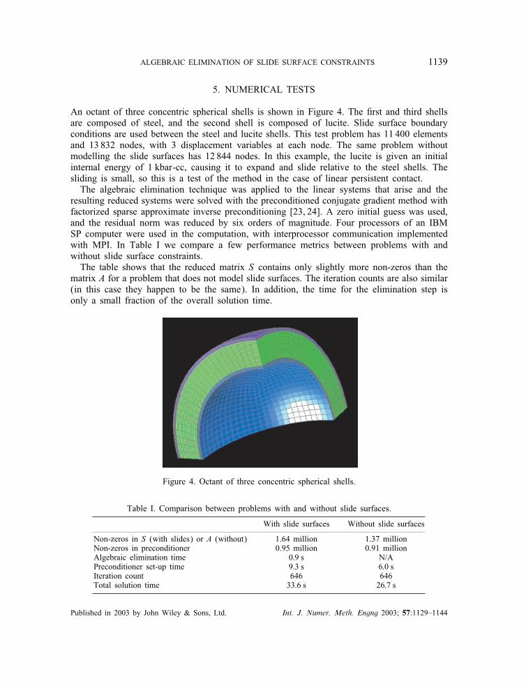
An octant of three concentric spherical shells is shown in Figure 4. The �rst and third shellsare composed of steel, and the second shell is composed of lucite. Slide surface boundaryconditions are used between the steel and lucite shells. This test problem has 11 400 elementsand 13 832 nodes, with 3 displacement variables at each node. The same problem withoutmodelling the slide surfaces has 12 844 nodes. In this example, the lucite is given an initialinternal energy of 1 kbar-cc, causing it to expand and slide relative to the steel shells. Thesliding is small, so this is a test of the method in the case of linear persistent contact.The algebraic elimination technique was applied to the linear systems that arise and the

resulting reduced systems were solved with the preconditioned conjugate gradient method withfactorized sparse approximate inverse preconditioning [23, 24]. A zero initial guess was used,and the residual norm was reduced by six orders of magnitude. Four processors of an IBMSP computer were used in the computation, with interprocessor communication implementedwith MPI. In Table I we compare a few performance metrics between problems with andwithout slide surface constraints.The table shows that the reduced matrix S contains only slightly more non-zeros than the

matrix A for a problem that does not model slide surfaces. The iteration counts are also similar(in this case they happen to be the same). In addition, the time for the elimination step isonly a small fraction of the overall solution time.

Figure 4. Octant of three concentric spherical shells.

Table I. Comparison between problems with and without slide surfaces.

With slide surfaces Without slide surfaces

Non-zeros in S (with slides) or A (without) 1.64 million 1.37 millionNon-zeros in preconditioner 0.95 million 0.91 millionAlgebraic elimination time 0:9 s N/APreconditioner set-up time 9:3 s 6:0 sIteration count 646 646Total solution time 33:6 s 26:7 s


1140 E. CHOW ET AL.

6. EXTENSION TO MORE GENERAL CONSTRAINTS

6.1. Intersecting constrained surfaces

For general constraints, it is not always possible to �nd a partitioning of the constrainedvariables into independent and dependent sets such that the dependent variables are purelydependent. Algebraically, this means that it may be impossible to reorder the columns andpartition GT into [BT; DT] such that D is diagonal. However, the algebraic elimination pro-cedure can still be economical if the inverse of D is sparse, e.g. when D is a block diagonalmatrix.A complete set of purely dependent variables cannot be found, for example, when two slide

surfaces intersect at a T. Figure 5 shows this case, which is actually treated as three slidesurfaces. Master and slave sides are chosen for each slide surface, and these are marked inthe �gure. Arrows in the �gure indicate that a slave node is dependent on a master node.Node 2 is a slave node for one slide surface, but is a master node for another. Also, node 5is a slave node for two slide surfaces. Nodes 2 and 5 are not purely dependent nodes.For intersecting slide surfaces, however, it is possible to partition the variables such that

D is block diagonal. Consider the following procedure for selecting the dependent variables,which corresponds to choosing columns of GT to form D. In this discussion, we will notdi�erentiate between variables and nodes, i.e. we consider a scalar problem.We start by choosing all slave nodes to be in the dependent set. If a slave node is not

purely dependent, then it falls under one of these two cases:

1. the node is a slave in one constraint and a master in one or more other constraints,2. the node is a slave node in more than one constraint.

In the �rst case, if a slave node is also a master in k constraints, then D will contain ablock of size (k+1)× (k+1) since the column of GT corresponding to the slave node hask+1 non-zeros. Nothing needs to be done in this case.In the second case, there are more constraints than slave nodes and one or more master

nodes must also be selected for the dependent set. Let s1 be a slave node that participates in

4

5 6

7 9

1

23

8 10

slavemastermaster

slave

mas

ter

slav

e

2 5 6

9

41

3

87 10

Figure 5. Intersecting slide surfaces. Figure 6. Graph of QQT.



constraints c1 and c2. A master node must be chosen from the master nodes in c1 or c2 sothat D will be non-singular. If the master node is a node that participates in k constraints,then D will contain block of size k × k; master nodes with small k should be preferred. Ifs1 is a slave node in more than two constraints, then two or more master nodes need to beselected simultaneously. Here, master nodes should be selected so that the total number ofnew constraints involved is minimized.In summary, the dependent set should be composed of all the slave nodes and selected

master nodes as described in the second case. The blocks formed in D may overlap so thatthe actual blocks may be larger than the sizes mentioned. This procedure is e�ective, butbecause of possible overlapping blocks, it is not optimal in the sense that the smallest blocksare found.

6.2. General constraints

In the case where the constraints are even more general, a block diagonal D can often stillbe found. In this section, we develop a graph theoretic framework for partitioning GT so thatD is block diagonal with small blocks.De�ne the binary matrix QT such that {QT}ij=1 if and only if constraint i involves

node j (which is either a master or slave node). The matrix QT contains m rows and ncolumns, where m is the number of constraints and n is the total number of slave and masternodes. For the geometry in Figure 5, we have the matrix

QT =

1 1 : 1 : : : : : :

1 1 : : 1 : : : : :

: : : : 1 : : : 1 1

: : : : : 1 : : 1 1

: 1 : : : : 1 1 : :

: : 1 : : : 1 1 : :

(14)

The matrix QQT contains a non-zero at (i; j) if and only if nodes i and j are involved inthe same constraint. The graph of QQT, denoted by G(QQT), will be helpful to understandthe partitioning problem at hand. For QT given by (14), G(QQT) is shown in Figure 6.A clique is a subgraph such that every vertex in the subgraph has an edge to every other

vertex in the subgraph. A maximal clique is a clique such that no vertex can be addedto the clique to form a larger clique. The graph G(QQT) contains m maximal cliques, eachcorresponding to a constraint, and the vertices of each clique correspond to the nodes involvedin the constraint. The partitioning problem is to select m nodes (or equivalently, vertices) suchthat D is block diagonal with small blocks.

Fact 6.1If an independent set of m vertices exists in G(QQT), then QT can be partitioned into [QT1 ; Q

T2 ]

such that QT2 is a diagonal matrix.

An independent set of size m may not exist. Further, �nding this independent set is equivalentto the maximum independent set problem, which is NP-hard.


1142 E. CHOW ET AL.

2 5 6

9

41

3

87 10

2 5 6

9

41

3

87 10

Figure 7. Selected vertices in G(QQT), formingthree 2× 2 blocks in D.

Figure 8. Selected vertices in G(QQT), formingtwo 1× 1 blocks and one 4× 4 block in D.

Fact 6.2A vertex from each maximal clique in G(QQT) must be selected, otherwise D will be singular.

Fact 6.3A connected set of k selected vertices in G(QQT) will form a block of size exactly k × k inD.

Fact 6.4Let Cj denote the number of maximal cliques in G(QQT) that vertex j belongs to. Selectingthis vertex for the dependent set will form a block of size at least Cj ×Cj in D.The partitioning problem may be solved, for example, by algorithms that try to select

vertices with small Cj. For example, m vertices with the smallest Cj may be selected to formthe dependent set. Figure 7 is a possible solution with this strategy for the graph of Figure6. Three vertices with Cj=1 are selected (solid circles) and three vertices with Cj=2 areselected (grey circles). For comparison, Figure 8 shows a situation where all the verticescorresponding to slave nodes (solid circles) are selected �rst, as suggested in the previoussubsection. Here, the solution is worse because D will contain a large 4× 4 block. Selectingvertices with small Cj is a poor algorithm for many other problems, however. We intend tofurther study the partitioning problem using this graph theoretic framework in a future paper.

6.3. Dense rows in GT

Dense rows in GT occur when constraints involve every variable of the problem, and makethe algebraic elimination technique very costly. As an alternative, these rows may be omittedfrom the elimination. Consider the partitioning of the matrix in (6) into[

A B

BT 0

]

where BT represents dense or relatively full rows and A represents the remainder of theproblem with sparse constraints. The algebraic elimination technique is only applied to A. Ifthe number of rows in BT is small, the reduced system based on the matrix BTA

−1B may be



solved iteratively. The reduced matrix is not formed and an iterative method for inde�nitesystems is required. Each iteration involves a solve with A which in turn involves a solve witha positive de�nite matrix. If the number of rows in BT is very small as in many applications,then very few iterations may be required.

7. CONCLUDING REMARKS

We have been regularly using the algebraic elimination technique described in this paper forsymmetric problems and have not encountered any di�culties with very poorly conditionedreduced matrices. The extension to more general constraints in Section 6 may be very valuable,and in future research we intend to develop and test algorithms based on these ideas.

ACKNOWLEDGEMENTS

The authors are grateful to Ivan Otero and John Ruge who formulated the implicit slide surface con-straints. The authors also wish to thank Colin Aro and Juliana Hsu, who participated in testing ouroriginal implementation of the software, and Mark Adams, John Lewis, Ali Pinar, Gene Poole, PanayotVassilevski, and Alan Williams for helpful discussions. Finally, we are grateful to the anonymous ref-erees for their comments which improved the presentation of this paper. This work was performedunder the auspices of the U.S. Department of Energy by University of California Lawrence LivermoreNational Laboratory under contract No. W-7405-Eng-48.

REFERENCES

1. Hallquist JO, Goudreau GL, Benson DJ. Sliding interfaces with contact-impact in large-scale Lagrangiancomputations. Computer Methods in Applied Mechanics and Engineering 1985; 51:107–137.

2. Carpenter NJ, Taylor RL, Katona MG. Lagrange constraints for transient �nite element surface contact.International Journal for Numerical Methods in Engineering 1991; 32:103–128.

3. Belytschko T, Moes N, Usui S, Parimi C. Arbitrary discontinuities in �nite elements. International Journal forNumerical Methods in Engineering 2001; 50:993–1013.

4. Rebel G, Park KC, Felippa CA. A contact-impact formulation based on localised Lagrange multipliers:formulation and application to two-dimensional problems. International Journal for Numerical Methods inEngineering 2002; 54:263–297.

5. Simo JC, Laursen TA. An augmented Lagrangian treatment of contact problems involving friction. Computersand Structures 1992; 42:97–116.

6. Laursen TA, Maker BN. An augmented Lagrangian quasi-Newton solver for constrained non-linear �nite elementapplications. International Journal for Numerical Methods in Engineering 1995; 38:3571–3590.

7. Pietrzak G, Curnier A. Large deformation frictional contact mechanics: continuum formulation and augmentedLagrange treatment. Computer Methods in Applied Mechanics and Engineering 1999; 177:351–381.

8. Cook RD, Malkus DS, Plesha ME. Concepts and Applications of Finite Element Analysis. 3rd edn. Wiley:New York, 1989.

9. Gallagher RH. Finite Element Analysis Fundamentals. Prentice-Hall: Englewood Cli�s, NJ, 1975.10. Curiskis JI, Valliappan S. A solution algorithm for linear constraint equations in �nite element analysis.

Computers and Structures 1978; 8:117–124.11. Abel JF, Shephard MS. An algorithm for multipoint constraints in �nite element analysis. International Journal

for Numerical Methods in Engineering 1979; 14:464–467.12. Saint-Georges P, Notay Y, Warz�ee G. E�cient iterative solution of constrained �nite element analyses. Computer

Methods in Applied Mechanics and Engineering 1998; 160:101–114.13. Gill PE, Murray W. Numerical Methods for Constrained Optimization. Academic Press: London, 1974.14. Gould NIM, Hribar ME, Nocedal J. On the solution of equality constrained quadratic programming problems

arising in optimization. SIAM Journal on Scienti�c Computing 2001; 23:1375–1394.15. Arrow K, Hurwicz L, Uzawa H. Studies in Nonlinear Programming. Stanford University Press: Stanford, CA,

1958.


1144 E. CHOW ET AL.

16. Elman HC, Golub GH. Inexact and preconditioned Uzawa algorithms for saddle point problems. SIAM Journalon Numerical Analysis 1994; 31:1645–1661.

17. Bank RE, Welfert BD, Yserentant H. A class of iterative methods for solving saddle point problems. NumerischeMathematik 1990; 56:645–666.

18. Axel Klawonn. Preconditioners for Inde�nite Problems. Ph.D. Thesis, Westf�alischen Wilhelms-Universit�atM�unster, 1995.

19. Murphy MF, Golub GH, Wathen AJ. A note on preconditioning for inde�nite linear systems. SIAM Journalon Scienti�c Computing 2000; 21:1969–1972.

20. Keller C, Gould NIM, Wathen AJ. Constraint preconditioning for inde�nite linear systems. SIAM Journal onMatrix Analysis and Applications 2000; 21:1300–1317.

21. Wilkinson JH. The Algebraic Eigenvalue Problem. Oxford University Press: Oxford, 1965.22. Parter SV. The use of linear graphs in Gauss elimination. SIAM Review 1961; 3:119–130.23. Chow E. A priori sparsity patterns for parallel sparse approximate inverse preconditioners. SIAM Journal on

Scienti�c Computing 2000; 21:1804–1822.24. Chow E. Parallel implementation and practical use of sparse approximate inverses with a priori sparsity patterns.

International Journal of High Performance Computing Applications 2001; 15:56–74.


algebraic elimination of slide surface constraints in implicit structural analysis

Documents