alemayehu geda note on open economy macroeconomic (msc/ma class) outline of the lecture (i)...
TRANSCRIPT

ADVANCED MACROECONOMICS I MSC
Alemayehu Geda Email: [email protected]
Web Page: www.alemayehu.com
Lecture 2
Consumption and Saving Theories
Addis Ababa University
Departement of Economics
MSc/MA Program
2014

Lecture Note on Open Economy
Macroeconomic (MSc/MA Class)
Outline of the Lecture
(i) Background about ???Theory
Alemayehu Geda
Dept. of Economics,
Addis Ababa University, 2014-2015
E-mail [email protected] &
web : www.Alemayeh.com

I. Background to the Theories

II. Aggregate Supply Side Issues
The objective of this part of the lecture is to show that the open economy variables , net exports, affects the aggregate economy not only directly but also indirectly through the sourcing of absorption (C+I+G).
The second objective of this part of the lecture is to derive the Marshall-Learner condition from the first principle. This is important to show not only the importance of the magnitude of export and import elasticities but also the initial level of BoP
deficit to make exchange rare policy effective.
Up to now we have assumed domestic and foreign prices are constant (ie. P=P*=1, which is a horizontal supply curve.
This might be true in the short run but we need to add the supply side to our Mundel-Fleming Model (Mead-Mundel-Fleming model) – this will give it a micro foundation.

II. Aggregate Supply Side Issues
For this purpose we use the model of Argy & Salop (1979),
Armington (1969) and Branson and Rotembert (1980) to show
the importance of the supply side issue.
We restrict our analysis to the case of perfect capital mobility
and flexible exchange rate.
The Armington Approach Since we are now modeling the supply side we need to be
precise about the various prices indices as well as the source of
goods that are used in the economy.
Broadly there are two goods (domestic and foreign) with
corresponding prices (domestic and foreign prices). We assumed
these goods to be imperfect substitutes.

II. Aggregate Supply …Cont’d
Real HH consumption and Investment are determined by the usual macro relationships
Regarding the sourcing of these goods Armington assumed that these goods, say C is “constructed” out of domestic and foreign goods through Cobb-Douglass relationships as:
𝐶 = 𝐶𝑑𝛼 𝐶𝑓
1−𝛼 [1]
Since HH as rational economic agents want to get C as cheaply as possible they will stand to optimize their spending function which is given as:
𝑃𝑐𝐶 = 𝑃𝐶𝑑 + 𝐸𝑃∗𝐶𝑓 [2]

II. Aggregate Supply …Cont’d
The HH can obtain the optimal ration between domestic and foreign goods by optimizing the following objective function as:
𝑀𝑖𝑛 𝑃𝑐𝐶 = 𝑃𝐶𝑑 + 𝐸𝑃∗𝐶𝑓 + 𝜆 𝐶 − 𝐶𝑑𝛼𝐶𝑓
1−𝛼
[! To be done: work out the optimization from the lecture here]
the first order condition for this will offer the following solution:
𝐶𝑑
𝐶𝑓=
𝛼
1−𝛼
𝐸𝑃∗
𝑃 [3]

II. Aggregate Supply Side Issues
The result in equation [3] shows that sourcing consumption
domestically directly related to the foreign to domestic price ratio
(the converse holds for sourcing from foreign countries)
Solving Eqn [3] for EP*Cf and inserting the result into the objective
function Eqn [2] (& similar procedure for EP*Cf)yields:
𝐶𝑑 =𝛼𝑃𝑐𝐶
𝑃 and 𝐶𝑓 =
(1−𝛼)𝑃𝑐𝐶
𝐸𝑃∗ [4]
Again substituting this result into the CD formulation (Eqn 1) we can
get an expression for the CPI [Pc]:
𝐶 =𝛼𝑃𝑐𝐶
𝑃
𝛼 (1−𝛼)𝑃𝑐𝐶
𝐸𝑃∗
1−𝛼=𝛼𝛼(1 − 𝛼)(1−𝛼)𝑃𝑐𝐶𝑃
−𝛼 𝐸𝑃∗ −(1−𝛼)

II. Aggregate Supply Side Issues
This implies the CPI [Pc]:
𝑃𝑐 = Ω0𝑃𝛼 𝐸𝑃∗ (1−𝛼) [5]
Where: Ω0 = 𝛼𝛼(1 − 𝛼)(1−𝛼)−1
> 0
By substituting [5] into [4] and taking C as C=c(Y), we get:
[6]
α/(1- α ) Pc C
Nb: Y raises both Cd & Cf; while EP*/P determines where to buy goods to be consumed.
Similar procedure offers similar equation for I & G as:

II. Aggregate Supply Side Issues
[7]
Depicting real exports by EX - sold at the same domestic price (P), and spending on imports being EP*(Cf+If+Gf), the NI identity could be given by:

II. Aggregate Supply Side Issues
[8]

II. Aggregate Supply Side Issues
The Marshall-Learner Condition
Let us assume the real net exports are given by:
[9]
If we assume further, as before, the demand for exports
depends on real exchange rare (EP*/P)=Q, we have:
[10]
Thus, we can have the net export function as:
𝐸𝑋0𝑄𝛽 − 𝑄(1 − 𝛼)Ω0𝑄
−𝛼 𝐴 𝑟, 𝑌 + 𝐺 [11]
Where M is based on Eqns [6] and [7]
Note the following that follows from Eqn [11]:

II. Aggregate Supply Side Issues
From Eqn [11] follows:
(1) Domestic absorption, not just aggregate demand, appears in the
net export function or Eq [11]
(2) Since domestic absorption depends on interest rate and some
investment goods are imported, the BP curve has a positive slop even
under imperfect capital mobility. [eg. I M of IfNTrade surplus
To restore equilibrium on NTrade Y (& hence M) must rise [M,Y ]
Having Eqn [11] we can now be more precise abou the Marshall-
Lerner condition by differentiate Eqn [11] wrt Q and dividing through
by Y, holding A+G constant. This gives:
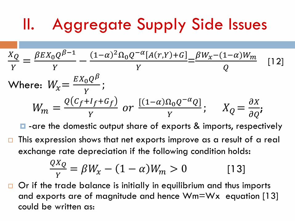
II. Aggregate Supply Side Issues
𝑋𝑄
𝑌=
𝛽𝐸𝑋0𝑄𝛽−1
𝑌−
1−𝛼 2Ω0𝑄−𝛼 𝐴 𝑟,𝑌 +𝐺
𝑌=𝛽𝑊𝑥−(1−𝛼)𝑊𝑚
𝑄 [12]
Where: 𝑊𝑥=𝐸𝑋0𝑄
𝛽
𝑌;
𝑊𝑚 =𝑄 𝐶𝑓+𝐼𝑓+𝐺𝑓
𝑌 𝑜𝑟
[ 1−𝛼 Ω0𝑄−𝛼𝑄]
𝑌; 𝑋𝑄=
𝜕𝑋
𝜕𝑄;
-are the domestic output share of exports & imports, respectively
This expression shows that net exports improve as a result of a real
exchange rate depreciation if the following condition holds: 𝑄𝑋𝑄
𝑌= 𝛽𝑊𝑥 − 1 − 𝛼 𝑊𝑚 > 0 [13]
Or if the trade balance is initially in equilibrium and thus imports and exports are of magnitude and hence Wm=Wx equation [13] could be written as:

II. Aggregate Supply Side Issues
= 𝛽𝑊𝑥 − 1 − 𝛼 𝑊𝑥 > 0
= 𝑊𝑥 𝛽 − 1 − 𝛼 > 0
=⇒ 𝛽 + 𝛼 > 10
Thus, Eqn [13], ie the condition for the improvement in NX,
will be true only if the above condition [Eqn 14] is satisfied.
This is what is referred as the Marshall-Learner condition: Only when
the sum of the elasticity of imports and exports is greater than 1
deprecation/devaluation could improve the trade balance.
Note that this condition requires initial equilibrium if so we do not
get this result (! Many African countries are in BoP disequilibrium)
Read John Weeks’ critique of this theory and the MF model (! John
says the theory is wrong and this doesn’t hold in LDCs’ at all)

II. Aggregate Supply Side Issues
A Brief View of the Overshooting Model
(The Dornbusch Model) The fundamental point in the overshooting model is that yield differential
b/n domestic and foreign investment depends not only on interest rate
differential but also on what is expected to happen to the exchange rate
in the period of investment.
𝑌𝑖𝑒𝑙𝑑 𝑔𝑎𝑝 = 1 + 𝑟 − 1 − 𝑟∗𝐸𝑒1𝐸0
= 1 + 𝑟 − 1 − 𝑟∗Δ𝐸𝑒
𝐸0
= 1 + 𝑟 − [ 1 + 𝑟∗ +Δ𝐸𝑒
𝐸0+𝑟∗
Δ𝐸𝑒
𝐸0] ≈ [𝑟 −(𝑟∗ +
Δ𝐸𝑒
𝐸0)]
Ignoring the last term which is a multiplication of fractions.
In a continuous time this is written as 𝑦𝑖𝑒𝑙 𝑔𝑎𝑝 = 𝑟 − (𝑟∗+𝑒𝑒 )

II. Aggregate Supply Side Issues
In the case of prefect capital mobility, arbitrage will ensure that the
yield differential is eliminate, in which case the above formulation is
reduced to the famous uncovered interest parity [UIP] condition:
𝑟 = (𝑟∗+𝑒𝑒 )
In the Dornbusch model, the UIP condition is assumed to hold
continuously.
Ie. If r<r* then there need to be an equivalent expected rate of appreciation
of domestic currency to compensate for lower r (owing to the perfect arbitrage,
if I put my money in birr here with lower r, cf to r*,, then when I want to buy $ I
must at least buy a lot with that birr next time – appreciation of Birr)
Note also a point stressed in the Dornbusch model which says goods price is
sticky (adjust slowly) so adjustment first come through exchange rate.

II. Aggregate Supply Side Issues
We can get the intuition of the model form the following diagram:
Price
PPP
C G2
P2
G1
P1 A B
M1 M2
e1 e0 e2 Exchange rate
overvaluation
undervaluation
Excess SS
Excess DD

II. Aggregate Supply Side Issues
At the initial equilibrium (A) the MS is give by M1, the domestic price
by P1 and the interest rate by r1 (not shown). The goods market
equilibrium is given by G1 the purchasing power parity condition
which says P=eP* is given by PPP.
Let us assume unanticipated increase in Ms to M2 at time t1, say by
20%. In the long run every one expects price to go to P1. This enailts a
20% depreciation of the domestic currency from e1 to e0 to maintain
the long run PPP at C.
However, the Dornbusch model says things are different in the short run
where prices are sticky and exchanger rate and money market are
not. Thus
At P1 the increase in MS (from M1 to M2) entails an excess SS of
money that will be willingly be held only if r is lowered from r1 to r2
(not shown)
II. Aggregate Supply Side Issues
This implies the new domestic interest rate (r2) is lower than r*
This in turn implies, speculators will require appreciation of the
domestic currency to compensate for the decline in r1 to that of r2.
For this reason e1 will jump (depreciate) from e1 to e2 at B,
overshooting its long run value of e0 at C.
It has to overshoot because it is only by the depreciation by
more than 20% (above e0) that there can be an expected
appreciation of domestic currency to compensate for the lower
interest rate on domestic assets (bonds).
There are various forces that bring back the economy back to the
long run point “C” following this monetary policy and short run
event that put the economy at “B”.

II. Aggregate Supply Side Issues
(1st ) the lower interest rate encourages investment and hence agg DD
(2nd ) The depreciation of the exchange rate to e2 encouraged exports
and discourage imports (and hence raises Agg DD)
This shifts Agg DD from G1 to G2.
As output is fixed this will lead to a rise in price form P1 to P2; and also
an exchange rate appreciation from e2 to e0.
(Expected appreciation is matched by actual appreciation)
Over time the economy movers to C where e0, P2, M2 &G2 prevail.
In the meant time interest rate raises from r2 to its original level r1 (not
shown in the figure) – so once again there is neither an expected
appreciation nor depreciation of the domestic currency.
[See the summary Figure in the next slide - & End of Lecture]

Dynamics of the Overshooting (Dornbusch) Model

End of Lecture